Monthly and seasonal streamflow forecasts using rainfall-runoff modeling and POAMA predictions

E. Wanga, H. Zhenga, F. Chiewa, Q. Shaob, J. Luoa,c, QJ Wangd

a CSIRO Water for a Healthy Country Flagship (WfHC) / CSIRO Land and Water, GPO Box 1666, Black Mountain, ACT 2601, Australia; bCSIRO Mathematics, Informatics and Statistics, Private Bag 5, Wembley,

WA 6913; cCollege of applied meteorology, Nanjing University of Information Science & Technology, Nanjing, China; dCSIRO (WfHC) / CSIRO Land and Water, PO Box 56, Highett, VIC 3190, Australia

Email: enli.wang@csiro.au

Abstract: Improved streamflow forecasts a month or season ahead are essential for water resource management and planning. This paper explored the skills of forecasts for monthly and three-monthly total streamflows with a dynamic approach using a conceptual rainfall-runoff model SIMHYD for 31 catchments located in east Australia. For all the catchments, the SIMHYD was calibrated in a moving mode, i.e. using all the data prior to the forecast year. Retrospective forecasts of streamflow totals were generated from 1981 onwards using the calibrated SIMHYD model together with three types of forcings:

• The observed daily rainfall – this option uses observed (real) rainfall data, the prediction skill of the model reflects the performance of the model in the verification period with real forcings, i.e., the top limit of the skills of the model-based forecasting.

• The daily rainfall data from all the years prior to the prediction year. For example, if there were 50 years of data available before the prediction year, the model was run 50 times, each with the daily rainfall data from each of the previous 50 year. An ensemble of 50 forecasts of daily streamflow was generated.

• The donwnscaled rainfall predictions from the Predictive Ocean Atmosphere Model for Australia (POAMA). An ensemble of 11 daily rainfall series for the prediction period from 1985 to 2006 were generated through downscaling POAMA forecasts (10 ensemble forecasts with the ensemble mean) using an analogue approach.

The results show that the SIMHYD model was able to capture the rainfall-runoff relationships in majority of months/seasons of studied catchments, once it was properly calibrated. However, the model performance varied in different months/seasons of the year and across catchments. It was relatively poorer in drier period of the year, i.e, winter-spring time in the northern catchments and summer-autumn time in the southern catchments. The dynamic forecasting approach based on conceptual rainfall-runoff modelling provides a potential way to improve streamflow forecasting at monthly and seasonal lead time in east Australia. Using POAMA forecasts as forcing for the rainfall-runoff model improved the forecasting skills as compared to using forcing sampled from history for monthly streamflow forecasts, but not for three-monthly forecasts. Across all the study catchments, use of POAMA ensemble as forcing led to an increase in total number of months with NSE>0.0 by 14% (164 to 187 months with NSE>0.0), but a decrease by 9% (112 to 102 months with NSE>0.0) for three-monthly forecasts. Possible improvements in forecasting skills through further bias-correction approaches are also discussed

Keywords: Decision Support System (DSS), Coastal Catchment Initiative (CCI), water quality

19th International Congress on Modelling and Simulation, Perth, Australia, 12–16 December 2011 http://mssanz.org.au/modsim2011

3441

Wang et al., Monthly and seasonal streamflow forecasts using rainfall-runoff modelling and POAMA outputs

1. INTRODUCTION

Improved seasonal water forecasting through statistical, dynamical or hybrid methods is one of the main research areas identified in Australia’s water resources research. The statistical approach to seasonal streamflow forecasting has been explored decades ago (Chiew and McMahon, 2002; Maurer and Lettenmaier, 2003; Ruiz et al, 2007, Chowdhury and Sharma, 2009), and has been further progressed recently. A Bayesian joint probability (BJP) approach, which combines climate indices and antecedent flows to forecast streamflow a season ahead, has been developed and tested at multiple sites in Australia (Wang et al, 2009) and to select predictors (Robertson and Wang, 2009). It has been found to provide useful forecasting skills in southeast Australian catchments and has become operational at the Australian Bureau of Meteorology (BoM) since December 2010 for seasonal flow forecasting.

The dynamical forecasting approach combines hydrologic modelling with forecast or re-sampled meteorological forcings, such as rainfall and potential evapotranspiration (PET), to forecast future streamflow. It is still in a pilot phase in Australia (Wang et al, 2011; Teng et al, 2011), although the approach has been explored since the early 1970s (Linsley et al, 1975) and is operationally used in the ensemble streamflow prediction (ESP) framework currently run by the National Weather Service (NWS) in the USA (Day, 1985; Wood et al, 2005). In ESP, a hydrologic model with ‘known’ catchment initial conditions is forced by an ensemble of forcing variables re-sampled from historical climate sequences or GCM predictions to generate probabilistic forecasts of future streamflow. As compared with historical ensemble inputs, Wood et al (2005) showed that unconditional (all years) GCM forecasts for regionally averaged variables did not improve streamflow forecasts in the USA. However, during strong ENSO years, forecasts may or may not benefit from using GCM forecasts, depending on regions where the ENSO tele-connection is strong or weak. In Australia, preliminary investigation of ESP approach with historical ensemble forcing in selected catchments in East Australia showed useful skills for monthly and three-monthly forecasts of streamflow totals, for the months and seasons following the wet season (Wang et al, 2011). Recently, efforts have been made to downscale, with bias-correction, the predictions of the Predictive Ocean Atmosphere Model for Australia (POAMA) (Shao et al, 2010), which enables the dynamic forecasting of streamflow with the forecast forcings (from POAMA), in addition to historical ensemble forcings.

The objectives of this paper are to use data from 31 catchments in east Australia to quantify the skills of the rainfall-runoff model-based forecasts of streamflow at monthly and seasonal scales using both historical ensemble forcings and forcings derived from POAMA downscaling.

2. DATA AND METHOD

2.1. Study Catchments and data

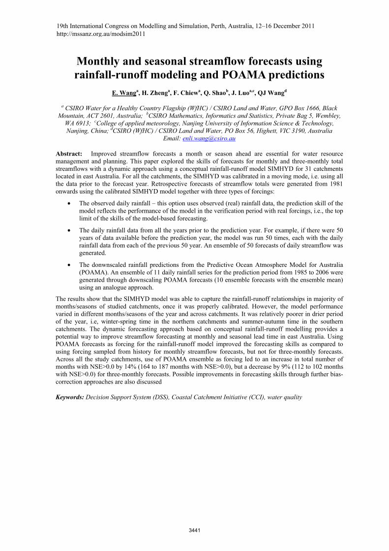
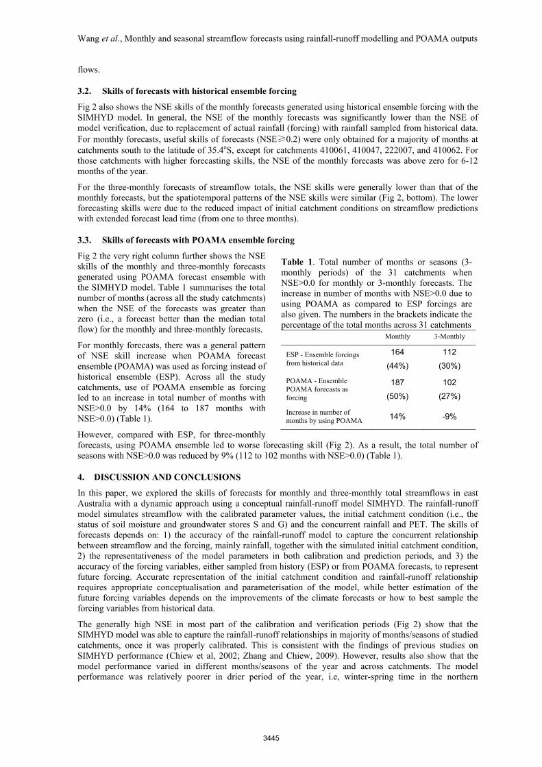
Thirty one unregulated catchments in east Australia (Fig 1) were selected for this study based on continuous data availability. Catchment details are summarized in Table 1. Daily streamflow data are obtained from relevant state government agencies (the Environment and Resource Management of Queensland Government for the Queensland stations, the NSW Water and Energy for the NSW gauges, and the Victorian Water Resources Data Warehouse), and have been checked for errors. Except the data from the three catchments in Queensland, all the other data are a sub-set of the catchment streamflow data as described in Vaze et al (2011).

Daily time series of maximum temperature, minimum temperature, incoming solar radiation, actual vapor pressure and precipitation at 0.05°×0.05°(~5km×5km) grid cells from the SILO Data Drill of the Queensland Department of Natural Resources and Water (www.nrw.gov.au/silo) (Jeffrey et al., 2001) are used. The SILO Data Drill provides surfaces of daily rainfall and other climate data interpolated from point measurements made by the Australian Bureau of Meteorology. Potential evapotranspiration (PET) are calculated by using the SILO data and the Priestley-Taylor model (Priestley and Taylor, 1972). Catchment averages of rainfall and PET were calculated and used for each catchment.

Figure 1. Location of the thirty one catchments selected for this study

3442

Wang et al., Monthly and seasonal streamflow forecasts using rainfall-runoff modelling and POAMA outputs

2.2. The SIMHYD model and its calibration

The SIMHYD model was used in this study (Chiew et al. 2002). It is a simple conceptual rainfall-runoff model with one soil moisture store (S) and one groundwater store (G), and runs at a daily time-step. The SIMHYD model is one of the most commonly used rainfall-runoff models in Australia, and has been applied in numerous studies within Australia and internationally, including the estimation of runoff in the National Land and Water Resources Audit and climate change impacts on runoff (Chiew and McMahon, 2002). The version used here has 9 parameters, seven from the original version and other two for routing simulation (Zhang and Chiew, 2009).

For all 31 study catchments, a progressive model calibration procedure was used to derive the parameters of the SIMHYD model. In the modelling process, assumptions were made that 1) at any given reference time, the future is unknown, and 2) model calibration can only be done using data collected before the reference time (because the future is unknown). To start, we set January 1, 1981 as the start time of model verification and forecasts for all the catchments. All the historical data before that date were used for model calibration, and the calibrated model was used to predict the streamflow in 1981. For each subsequent year, i.e., each year from 1982 to the last year of available data, the model was re-calibrated using all the data before the prediction/forecast year before it was used to predict/forecast streamflow in that year. This procedure ensures that for any given reference time, all the past data, but no future information, were used to calibrate the model.

For each forecast year, SIMHYD model was run continuously from the first year of available streamflow data to 31 December of the year before the prediction/forecast year. The Rosenbrock optimisation method (Manley, 1978) was used to maximise the Nash-Sutcliffe Efficiency (NSE) (Nash and Sutcliffe, 1970) on daily observed and simulated flows in the calibration period:

=

=

−

−−=

N

iOBS

tOBS

N

i

ttOBS

yy

yyNSE

1

2

1

2

)(

)(1 (1)

where yt and ytOBS are the simulated and observed daily streamflow, respectively.

OBSy is is the arithmetic

mean of the observed streamflow. N is the sample size, i.e., total days or months. The Nash-Sutcliffe efficiency expresses the proportion of variance of the observed streamflow that is accounted for by the model and provides a direct measure of the ability of the model to reproduce the observed streamflow. NSE = 1.0 indicates a perfect model being able to reproduce all the observed daily streamflows.

2.3. Model verification and ensemble forecasts

For each year (the prediction/forecast year) from 1981 onwards, the SIMHYD model was run with parameters derived using data from all previous years. Up to the 1st January of the prediction/forecast year, observed rainfall data were used to drive the model. In the prediction/forecast year, the following inputs were used to drive the model for verification and forecast modelling:

• The observed daily rainfall – this option uses observed (real) rainfall data, the prediction skill of the model reflects the performance of the model in the verification period with real forcings, i.e., the top limit of the skills of the model-based forecasting. This option is denoted as ‘Verification’

• The daily rainfall data from all the years prior to the prediction year. For example, if there were 50 years of data available before the prediction year, the model was run 50 times, each with the daily rainfall data from each of the previous 50 year. An ensemble of 50 forecasts of daily streamflow was generated. This option is denoted as ‘ESP’.

• The daily rainfall data generated using an analogue downscaling approach with POAMA forecasts – an ensemble of 11 daily rainfall series for the prediction period from 1985 to 2006 were generated through downscaling POAMA forecasts (10 ensemble forecasts with the ensemble mean). An analogue approach based on Timbal and Fernadez (2008), together with bias correction of POAMA climatology through a multivariate Box-Cox transformation (Shao and Li, 2010), was used for the downscaling of POAMA predictions. This option is denoted as ‘POAMA’

The above prediction and forecasts were done year by year for the entire period from 1981 to 2006. Daily streamflows were summed up to monthly total flows and three-monthly total flows starting from each of the

3443

Wang et al., Monthly and seasonal streamflow forecasts using rainfall-runoff modelling and POAMA outputs

12 months. The median of the ensemble forecasts using ESP and POAMA were calculated, and compared with the totals of the observed streamflows to evaluate the model performance and forecasting skills.

Different skill measures were used in the literature (Potts et al., 1996; Wilks, 2006; Wang et al., 2009) to evaluate forecasts. For forecasts across multiple months, seasons and sites, we feel that a skill score by comparing the skill gain against a reference forecast is most meaningful, easy to interpret and convenient, thus the NSE (equation 1) is also used here to evaluate the forecasting skills. We used the climatological median of the flow totals in the targeted month or 3-month period as the reference forecast. In this case the NSE calculated is the same as the skill score proposed by Wilks (2006). NSE=0 implies that the model predictions are the same as the climatological median, while a NSE>0 indicates a forecast better than the climatological median.

3. RESULTS

3.1. Model calibration and verification skills

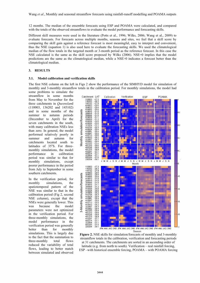
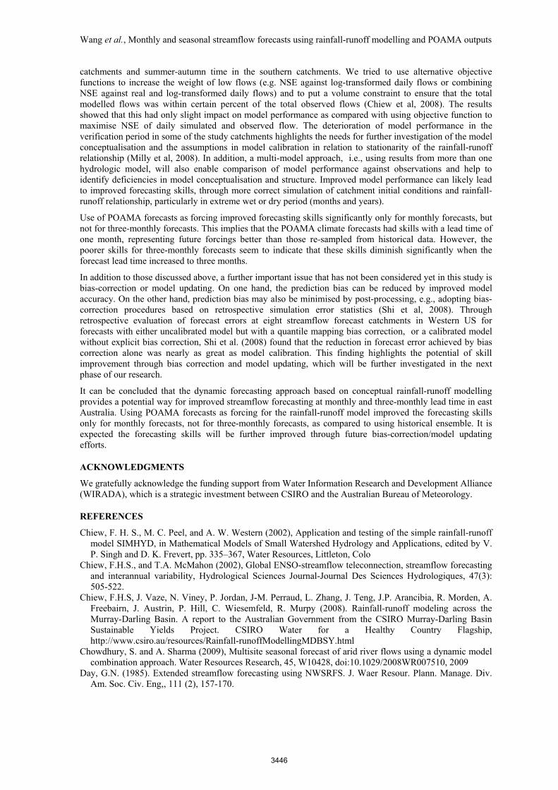
The first NSE column on the left in Figs 2 show the performance of the SIMHYD model for simulation of monthly and 3-monthly streamflow totals in the calibration period. For monthly simulations, the model had some problems to simulate the streamflow in some months from May to November for the three catchments in Queensland (110003, 136202 and 145102) and in some months of the summer to autumn periods (December to April) for the seven catchments in the south, with many calibration NSEs less than zero. In general, the model performed relatively poorly in summer and autumn for catchments located south to latitudes of 35oS. For three-monthly simulations, the model performance in calibration period was similar to that for monthly simulations, except poorer performance in the period from July to September in some southern catchments.

In the verification period, for monthly simulations, the spatiotemporal pattern of the NSE was similar to that in the calibration period (Fig 2, second NSE column), except that the NSEs were generally lower. This was because the model parameters were not optimized in the verification period. For three-monthly simulations, the model performance in the verification period was generally better than for monthly simulations. This is largely due to the fact that the summation to three-monthly total flows reduced the variability of total flows, leading to better match between simulated and observed

Mon

thly

sim

ulat

ion/

fore

cast

s3-

Mon

thly

sim

ulat

ion/

fore

cast

sM

onth

ly s

imul

atio

n/fo

reca

sts

3-M

onth

ly s

imul

atio

n/fo

reca

sts

Figure 2. NSE skills for simulation/forecasts of monthly and 3-monthly streamflow totals in the calibration, verification and forecasting periods

at 31 catchments. The catchments are sorted in an ascending order of latitude (e.g. from north to south). Verification – real rainfall forcing,

ESP –with historical ensemble forcing, POAMA – with POAMA forcing

3444

Wang et al., Monthly and seasonal streamflow forecasts using rainfall-runoff modelling and POAMA outputs

flows.

3.2. Skills of forecasts with historical ensemble forcing

Fig 2 also shows the NSE skills of the monthly forecasts generated using historical ensemble forcing with the SIMHYD model. In general, the NSE of the monthly forecasts was significantly lower than the NSE of model verification, due to replacement of actual rainfall (forcing) with rainfall sampled from historical data. For monthly forecasts, useful skills of forecasts (NSE≥0.2) were only obtained for a majority of months at catchments south to the latitude of 35.4oS, except for catchments 410061, 410047, 222007, and 410062. For those catchments with higher forecasting skills, the NSE of the monthly forecasts was above zero for 6-12 months of the year.

For the three-monthly forecasts of streamflow totals, the NSE skills were generally lower than that of the monthly forecasts, but the spatiotemporal patterns of the NSE skills were similar (Fig 2, bottom). The lower forecasting skills were due to the reduced impact of initial catchment conditions on streamflow predictions with extended forecast lead time (from one to three months).

3.3. Skills of forecasts with POAMA ensemble forcing

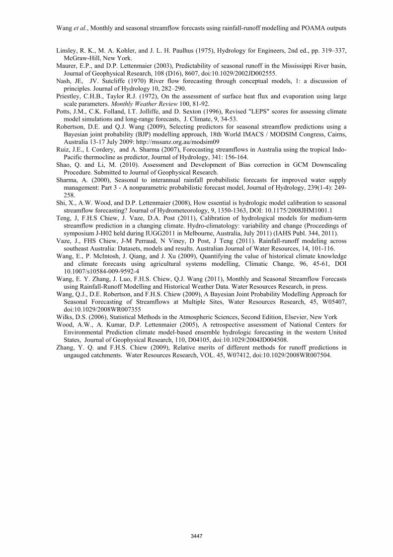
Fig 2 the very right column further shows the NSE skills of the monthly and three-monthly forecasts generated using POAMA forecast ensemble with the SIMHYD model. Table 1 summarises the total number of months (across all the study catchments) when the NSE of the forecasts was greater than zero (i.e., a forecast better than the median total flow) for the monthly and three-monthly forecasts.

For monthly forecasts, there was a general pattern of NSE skill increase when POAMA forecast ensemble (POAMA) was used as forcing instead of historical ensemble (ESP). Across all the study catchments, use of POAMA ensemble as forcing led to an increase in total number of months with NSE>0.0 by 14% (164 to 187 months with NSE>0.0) (Table 1).

However, compared with ESP, for three-monthly forecasts, using POAMA ensemble led to worse forecasting skill (Fig 2). As a result, the total number of seasons with NSE>0.0 was reduced by 9% (112 to 102 months with NSE>0.0) (Table 1).

4. DISCUSSION AND CONCLUSIONS

In this paper, we explored the skills of forecasts for monthly and three-monthly total streamflows in east Australia with a dynamic approach using a conceptual rainfall-runoff model SIMHYD. The rainfall-runoff model simulates streamflow with the calibrated parameter values, the initial catchment condition (i.e., the status of soil moisture and groundwater stores S and G) and the concurrent rainfall and PET. The skills of forecasts depends on: 1) the accuracy of the rainfall-runoff model to capture the concurrent relationship between streamflow and the forcing, mainly rainfall, together with the simulated initial catchment condition, 2) the representativeness of the model parameters in both calibration and prediction periods, and 3) the accuracy of the forcing variables, either sampled from history (ESP) or from POAMA forecasts, to represent future forcing. Accurate representation of the initial catchment condition and rainfall-runoff relationship requires appropriate conceptualisation and parameterisation of the model, while better estimation of the future forcing variables depends on the improvements of the climate forecasts or how to best sample the forcing variables from historical data.

The generally high NSE in most part of the calibration and verification periods (Fig 2) show that the SIMHYD model was able to capture the rainfall-runoff relationships in majority of months/seasons of studied catchments, once it was properly calibrated. This is consistent with the findings of previous studies on SIMHYD performance (Chiew et al, 2002; Zhang and Chiew, 2009). However, results also show that the model performance varied in different months/seasons of the year and across catchments. The model performance was relatively poorer in drier period of the year, i.e, winter-spring time in the northern

Table 1. Total number of months or seasons (3-monthly periods) of the 31 catchments when NSE>0.0 for monthly or 3-monthly forecasts. The increase in number of months with NSE>0.0 due to using POAMA as compared to ESP forcings are also given. The numbers in the brackets indicate the percentage of the total months across 31 catchments

Monthly 3-Monthly

ESP - Ensemble forcings from historical data

164

(44%)

112

(30%)

POAMA - Ensemble POAMA forecasts as forcing

187

(50%)

102

(27%)

Increase in number of months by using POAMA 14% -9%

3445

Wang et al., Monthly and seasonal streamflow forecasts using rainfall-runoff modelling and POAMA outputs

catchments and summer-autumn time in the southern catchments. We tried to use alternative objective functions to increase the weight of low flows (e.g. NSE against log-transformed daily flows or combining NSE against real and log-transformed daily flows) and to put a volume constraint to ensure that the total modelled flows was within certain percent of the total observed flows (Chiew et al, 2008). The results showed that this had only slight impact on model performance as compared with using objective function to maximise NSE of daily simulated and observed flow. The deterioration of model performance in the verification period in some of the study catchments highlights the needs for further investigation of the model conceptualisation and the assumptions in model calibration in relation to stationarity of the rainfall-runoff relationship (Milly et al, 2008). In addition, a multi-model approach, i.e., using results from more than one hydrologic model, will also enable comparison of model performance against observations and help to identify deficiencies in model conceptualisation and structure. Improved model performance can likely lead to improved forecasting skills, through more correct simulation of catchment initial conditions and rainfall-runoff relationship, particularly in extreme wet or dry period (months and years).

Use of POAMA forecasts as forcing improved forecasting skills significantly only for monthly forecasts, but not for three-monthly forecasts. This implies that the POAMA climate forecasts had skills with a lead time of one month, representing future forcings better than those re-sampled from historical data. However, the poorer skills for three-monthly forecasts seem to indicate that these skills diminish significantly when the forecast lead time increased to three months.

In addition to those discussed above, a further important issue that has not been considered yet in this study is bias-correction or model updating. On one hand, the prediction bias can be reduced by improved model accuracy. On the other hand, prediction bias may also be minimised by post-processing, e.g., adopting bias-correction procedures based on retrospective simulation error statistics (Shi et al, 2008). Through retrospective evaluation of forecast errors at eight streamflow forecast catchments in Western US for forecasts with either uncalibrated model but with a quantile mapping bias correction, or a calibrated model without explicit bias correction, Shi et al. (2008) found that the reduction in forecast error achieved by bias correction alone was nearly as great as model calibration. This finding highlights the potential of skill improvement through bias correction and model updating, which will be further investigated in the next phase of our research.

It can be concluded that the dynamic forecasting approach based on conceptual rainfall-runoff modelling provides a potential way for improved streamflow forecasting at monthly and three-monthly lead time in east Australia. Using POAMA forecasts as forcing for the rainfall-runoff model improved the forecasting skills only for monthly forecasts, not for three-monthly forecasts, as compared to using historical ensemble. It is expected the forecasting skills will be further improved through future bias-correction/model updating efforts.

ACKNOWLEDGMENTS

We gratefully acknowledge the funding support from Water Information Research and Development Alliance (WIRADA), which is a strategic investment between CSIRO and the Australian Bureau of Meteorology.

REFERENCES

Chiew, F. H. S., M. C. Peel, and A. W. Western (2002), Application and testing of the simple rainfall-runoff model SIMHYD, in Mathematical Models of Small Watershed Hydrology and Applications, edited by V. P. Singh and D. K. Frevert, pp. 335–367, Water Resources, Littleton, Colo

Chiew, F.H.S., and T.A. McMahon (2002), Global ENSO-streamflow teleconnection, streamflow forecasting and interannual variability, Hydrological Sciences Journal-Journal Des Sciences Hydrologiques, 47(3): 505-522.

Chiew, F.H.S, J. Vaze, N. Viney, P. Jordan, J-M. Perraud, L. Zhang, J. Teng, J.P. Arancibia, R. Morden, A. Freebairn, J. Austrin, P. Hill, C. Wiesemfeld, R. Murpy (2008). Rainfall-runoff modeling across the Murray-Darling Basin. A report to the Australian Government from the CSIRO Murray-Darling Basin Sustainable Yields Project. CSIRO Water for a Healthy Country Flagship, http://www.csiro.au/resources/Rainfall-runoffModellingMDBSY.html

Chowdhury, S. and A. Sharma (2009), Multisite seasonal forecast of arid river flows using a dynamic model combination approach. Water Resources Research, 45, W10428, doi:10.1029/2008WR007510, 2009

Day, G.N. (1985). Extended streamflow forecasting using NWSRFS. J. Waer Resour. Plann. Manage. Div. Am. Soc. Civ. Eng,, 111 (2), 157-170.

3446

Wang et al., Monthly and seasonal streamflow forecasts using rainfall-runoff modelling and POAMA outputs

Linsley, R. K., M. A. Kohler, and J. L. H. Paulhus (1975), Hydrology for Engineers, 2nd ed., pp. 319–337, McGraw-Hill, New York.

Maurer, E.P., and D.P. Lettenmaier (2003), Predictability of seasonal runoff in the Mississippi River basin, Journal of Geophysical Research, 108 (D16), 8607, doi:10.1029/2002JD002555.

Nash, JE, JV. Sutcliffe (1970) River flow forecasting through conceptual models, 1: a discussion of principles. Journal of Hydrology 10, 282–290.

Priestley, C.H.B., Taylor R.J. (1972), On the assessment of surface heat flux and evaporation using large scale parameters. Monthly Weather Review 100, 81-92.

Potts, J.M., C.K. Folland, I.T. Jolliffe, and D. Sexton (1996), Revised "LEPS" scores for assessing climate model simulations and long-range forecasts, J. Climate, 9, 34-53.

Robertson, D.E. and Q.J. Wang (2009), Selecting predictors for seasonal streamflow predictions using a Bayesian joint probability (BJP) modelling approach, 18th World IMACS / MODSIM Congress, Cairns, Australia 13-17 July 2009: http://mssanz.org.au/modsim09

Ruiz, J.E., I. Cordery, and A. Sharma (2007), Forecasting streamflows in Australia using the tropical Indo-Pacific thermocline as predictor, Journal of Hydrology, 341: 156-164.

Shao, Q. and Li, M. (2010). Assessment and Development of Bias correction in GCM Downscaling Procedure. Submitted to Journal of Geophysical Research.

Sharma, A. (2000), Seasonal to interannual rainfall probabilistic forecasts for improved water supply management: Part 3 - A nonparametric probabilistic forecast model, Journal of Hydrology, 239(1-4): 249-258.

Shi, X., A.W. Wood, and D.P. Lettenmaier (2008), How essential is hydrologic model calibration to seasonal streamflow forecasting? Journal of Hydrometeorology, 9, 1350-1363, DOI: 10.1175/2008JHM1001.1

Teng, J, F.H.S Chiew, J. Vaze, D.A. Post (2011), Calibration of hydrological models for medium-term streamflow prediction in a changing climate. Hydro-climatology: variability and change (Proceedings of symposium J-H02 held during IUGG2011 in Melbourne, Australia, July 2011) (IAHS Publ. 344, 2011).

Vaze, J., FHS Chiew, J-M Perraud, N Viney, D Post, J Teng (2011). Rainfall-runoff modeling across southeast Australia: Datasets, models and results. Australian Journal of Water Resources, 14, 101-116.

Wang, E., P. McIntosh, J. Qiang, and J. Xu (2009), Quantifying the value of historical climate knowledge and climate forecasts using agricultural systems modelling, Climatic Change, 96, 45-61, DOI 10.1007/s10584-009-9592-4

Wang, E. Y. Zhang, J. Luo, F.H.S. Chiew, Q.J. Wang (2011), Monthly and Seasonal Streamflow Forecasts using Rainfall-Runoff Modelling and Historical Weather Data. Water Resources Research, in press.

Wang, Q.J., D.E. Robertson, and F.H.S. Chiew (2009), A Bayesian Joint Probability Modelling Approach for Seasonal Forecasting of Streamflows at Multiple Sites, Water Resources Research, 45, W05407, doi:10.1029/2008WR007355

Wilks, D.S. (2006), Statistical Methods in the Atmospheric Sciences, Second Edition, Elsevier, New York Wood, A.W., A. Kumar, D.P. Lettenmaier (2005), A retrospective assessment of National Centers for

Environmental Prediction climate model-based ensemble hydrologic forecasting in the western United States, Journal of Geophysical Research, 110, D04105, doi:10.1029/2004JD004508.

Zhang, Y. Q. and F.H.S. Chiew (2009), Relative merits of different methods for runoff predictions in ungauged catchments. Water Resources Research, VOL. 45, W07412, doi:10.1029/2008WR007504.

3447