Monotone Submodular Maximization over a Matroid

via Non-Oblivious Local Search

Yuval Filmus∗ and Justin Ward†

December 30, 2013

Abstract

We present an optimal, combinatorial 1−1/e approximation algorithm for monotone submodular op-timization over a matroid constraint. Compared to the continuous greedy algorithm (Calinescu, Chekuri,Pal and Vondrak, 2008), our algorithm is extremely simple and requires no rounding. It consists of thegreedy algorithm followed by local search. Both phases are run not on the actual objective function, buton a related auxiliary potential function, which is also monotone and submodular.

In our previous work on maximum coverage (Filmus and Ward, 2012), the potential function givesmore weight to elements covered multiple times. We generalize this approach from coverage functionsto arbitrary monotone submodular functions. When the objective function is a coverage function, bothdefinitions of the potential function coincide.

Our approach generalizes to the case where the monotone submodular function has restricted curva-ture. For any curvature c, we adapt our algorithm to produce a (1−e−c)/c approximation. This matchesresults of Vondrak (2008), who has shown that the continuous greedy algorithm produces a (1 − e−c)/capproximation when the objective function has curvature c with respect to the optimum, and provedthat achieving any better approximation ratio is impossible in the value oracle model.

1 Introduction

In this paper, we consider the problem of maximizing a monotone submodular function f , subject to a singlematroid constraint. Formally, let U be a set of n elements and let f : 2U → R be a function assigning a valueto each subset of U . We say that f is submodular if

f(A) + f(B) ≥ f(A ∪B) + f(A ∩B)

for all A,B ⊆ U . If additionally f is monotone, that is f(A) ≤ f(B) whenever A ⊆ B, we say that f ismonotone submodular. Submodular functions exhibit (and are, in fact, alternately characterized by) theproperty of diminishing returns—if f is submodular then f(A ∪ x) − f(A) ≤ f(B ∪ x) − f(B) for allB ⊆ A. Hence, they are useful for modeling economic and game-theoretic scenarios, as well as variouscombinatorial problems. In a general monotone submodular maximization problem, we are given a valueoracle for f and a membership oracle for some distinguished collection I ⊆ 2U of feasible sets, and our goalis to find a member of I that maximizes the value of f . We assume further that f is normalized so thatf(∅) = 0.

We consider the restricted setting in which the collection I forms a matroid. Matroids are intimatelyconnected to combinatorial optimization: the problem of optimizing a linear function over a hereditaryset system (a set system closed under taking subsets) is solved optimally for all possible functions by thestandard greedy algorithm if and only if the set system is a matroid [32, 11].

∗yuvalf@cs.toronto.edu†J.D.Ward@dcs.warwick.ac.uk Work supported by EPSRC grant EP/J021814/1.

1

In the case of a monotone submodular objective function, the standard greedy algorithm, which takesat each step the element yielding the largest increase in f while maintaining independence, is (only) a 1/2-approximation [20]. Recently, Calinescu et al. [7, 34, 8] have developed a (1 − 1/e)-approximation for thisproblem via the continuous greedy algorithm, which is reminiscent of the classical Frank–Wolfe algorithm [21],producing a fractional solution. The fractional solution is rounded using pipage rounding [1] or swap rounding[10]. Recently, a fast variant of this algorithm running in time O(n2) has been designed by Ashwinkumarand Vondrak [3].

Feige [12] has shown that improving the bound (1 − 1/e) is NP-hard even if f is an explicity-givencoverage function (the objective function of an instance of maximum coverage). Nemhauser and Wolsey [30]have shown that any improvement over (1 − 1/e) requires an exponential number of queries in the valueoracle setting.

Following Vondrak [35], we also consider the case when f has restricted curvature. We say that f hascurvature c if for any two disjoint A,B ⊆ U ,

f(A ∪B) ≥ f(A) + (1− c)f(B).

When c = 1, this is a restatement of monotonicity of f , and when c = 0, linearity of f . Vondrak [35] hasshown that the continuous greedy algorithm produces a (1− e−c)/c approximation when f has curvature c.In fact, he shows that this is true even for the weaker definition of curvature with respect to the optimum.Furthermore, for this weaker notion of curvature, he has shown that any improvement over (1 − e−c)/crequires an exponential number of queries in the value oracle setting. The optimal approximation ratiofor functions of unrestricted curvature c has recently been determined to be (1 − c/e) by Sviridenko andWard [33], who use the non-oblivious local search approach described in this paper.

1.1 Our contribution

In this paper, we propose a conceptually simple randomized polynomial time local search algorithm forthe problem of monotone submodular matroid maximization. Like the continuous greedy algorithm, ouralgorithm delivers the optimal (1 − 1/e)-approximation. However, unlike the continuous greedy algorithm,our algorithm is entirely combinatorial, in the sense that it deals only with integral solutions to the problemand hence involves no rounding procedure. As such, we believe that the algorithm may serve as a gatewayto further improved algorithms in contexts where pipage rounding and swap rounding break down, such assubmodular maximization subject to multiple matroid constraints. Its combinatorial nature has anotheradvantage: the algorithm only evaluates the objective function on independent sets of the matroid.

Our main results are a combinatorial 1 − 1/e − ε approximation algorithm for monotone submodularmatroid maximization, running in time O(ε−3r4n), and a combinatorial 1 − 1/e approximation algorithmrunning in time O(r7n2), where r is the rank of the given matroid and n is the size of its ground set. Bothalgorithms are randomized, and succeed with probability 1− 1/n. Our algorithm further generalizes to thecase in which the submodular function has curvature c with respect to the optimum (see Section 2 for adefinition). In this case the approximation ratios obtained are (1− e−c)/c− ε and (1− e−c)/c, respectively,again matching the performance of the continuous greedy algorithm [35]. Unlike the continuous greedyalgorithm, our algorithm requires knowledge of c. However, by enumerating over values of c we are able toobtain a combinatorial (1− e−c)/c algorithm even in the case that f ’s curvature is unknown.1

Our algorithmic approach is based on local search. In classical local search, the algorithm starts at anarbitrary solution, and proceeds by iteratively making small changes that improve the objective function,until no such improvement can be made. A natural, worst-case guarantee on the approximation performanceof a local search algorithm is the locality ratio, given as min f(S)/f(O), where S is a locally optimal solution(i.e. a solution which cannot be improved by the small changes considered by the algorithm), O is a globaloptimum, and f is the objective function.

In many cases, classical local search may have a sub-optimal locality ratio, implying that a locally-optimal solution may be of significantly lower quality than the global optimum. For example, for monotone

1For technical reasons, we require that f has curvature bounded away from zero in this case.

2

submodular maximization over a matroid, the locality ratio for an algorithm changing a single element ateach step is 1/2 [20]. Non-oblivious local search, a technique first proposed by Alimonti [2] and by Khanna,Motwani, Sudan and Vazirani [26], attempts to avoid this problem by making use of a secondary potentialfunction to guide the search. By carefully choosing this auxiliary function, we ensure that poor local optimawith respect to the original objective function are no longer local optima with respect to the new potentialfunction. This is the approach that we adopt in the design of our local search algorithm. Specifically,we consider a simple local search algorithm in which the value of a solution is measured with respect toa carefully designed potential function g, rather than the submodular objective function f . We show thatsolutions which are locally optimal with respect to g have significantly higher worst-case quality (as measuredby the problem’s original potential function f) than those which are locally optimal with respect to f .

In our previous work [17], we designed an optimal non-oblivious local search algorithm for the restrictedcase of maximum coverage subject to a matroid constraint. In this problem, we are given a weighted universeof elements, a collection of sets, and a matroid defined on this collection. The goal is to find a collection ofsets that is independent in the matroid and covers elements of maximum total weight. The non-obliviouspotential function used in [17] gives extra weight to solutions that cover elements multiple times. That is, thepotential function depends critically on the coverage representation of the objective function. In the presentwork, we extend this approach to general monotone submodular functions. This presents two challenges:defining a non-oblivious potential function without referencing the coverage representation, and analyzingthe resulting algorithm.

In order to define the general potential function, we construct a generalized variant of the potentialfunction from [17] that does not require a coverage representation. Instead, the potential function aggregatesinformation obtained by applying the objective function to all subsets of the input, weighted according totheir size. Intuitively, the resulting potential function gives extra weight to solutions that contain a largenumber of good sub-solutions, or equivalently, remain good solutions in expectation when elements areremoved by a random process. An appropriate setting of the weights defining our potential function yieldsa function which coincides with the previous definition for coverage functions, but still makes sense forarbitrary monotone submodular functions.

The analysis of the algorithm in [17] is relatively straightforward. For each type of element in the universeof the coverage problem, we must prove a certain inequality among the coefficients defining the potentialfunction. In the general setting, however, we need to construct a proof using only the inequalities given bymonotonicity and submodularity. The resulting proof is non-obvious and delicate.

This paper extends and simplifies a previous work by the same authors. The paper [18], appearing inFOCS 2012, only discusses the case c = 1. The general case is discussed in [19], which appears in ArXiv.The potential functions used to guide the non-oblivious local search in both the unrestricted curvature case[18] and the maximum coverage case [17] are special cases of the function g we discuss in the present paper.2

An exposition of the ideas of both [17] and [19] can be found in the second author’s thesis [37]. In particular,the thesis explains how the auxiliary objective function can be determined by solving a linear program, bothin the special case of maximum coverage and in the general case of monotone submodular functions withrestricted curvature.

1.2 Related work

Fisher, Nemhauser and Wolsey [31, 20] analyze greedy and local search algorithms for submodular maxi-mization subject to various constraints, including single and multiple matroid constraints. They obtain someof the earliest results in the area, including a 1/(k + 1)-approximation algorithm for monotone submodularmaximization subject to k matroid constraints. A recent survey by Goundan and Schulz [24] reviews manyresults pertaining to the greedy algorithm for submodular maximization.

More recently, Lee, Sviridenko and Vondrak [29] consider the problem of both monotone and non-monotone submodular maximization subject to multiple matroid constraints, attaining a 1/(k + ε)-approx-

2The functions from [18, 19] are defined in terms of certain coefficients γ, which depend on a parameter E. Our definitionhere corresponds to the choice E = ec. We examine the case of coverage functions in more detail in Section 8.3.

3

imation for monotone submodular maximization subject to k ≥ 2 matroid constraints using local search.Feldman et al. [16] show that a local search algorithm attains the same bound for the related class ofk-exchange systems, which includes the intersection of k strongly base orderable matroids, as well as theindependent set problem in (k+ 1)-claw free graphs. Further work by Ward [36] shows that a non-obliviouslocal search routine attains an improved approximation ratio of 2/(k + 3)− ε for this class of problems.

In the case of unconstrained non-monotone maximization, Feige, Mirrokni and Vondrak [13] give a 2/5-approximation algorithm via a randomized local search algorithm, and give an upper bound of 1/2 in thevalue oracle model. Gharan and Vondrak [22] improved the algorithmic result to 0.41 by enhancing thelocal search algorithm with ideas borrowed from simulated annealing. Feldman, Naor and Schwarz [15] laterimproved this to 0.42 by using a variant of the continuous greedy algorithm. Buchbinder, Feldman, Naorand Schwartz have recently obtained an optimal 1/2-approximation algorithm [5].

In the setting of constrained non-monotone submodular maximization, Lee et al. [28] give a 1/(k+2+ 1k +

ε)-approximation algorithm for the case of k matroid constraints and a (1/5 − ε)-approximation algorithmfor k knapsack constraints. Further work by Lee, Sviridenko and Vondrak [29] improves the approximationratio in the case of k matroid constraints to 1/(k + 1 + 1

k−1 + ε). Feldman et al. [16] attain this ratiofor k-exchange systems. Chekuri, Vondrak and Zenklusen [9] present a general framework for optimizingsubmodular functions over downward-closed families of sets. Their approach combines several algorithms foroptimizing the multilinear relaxation along with dependent randomized rounding via contention resolutionschemes. As an application, they provide constant-factor approximation algorithms for several submodularmaximization problems.

In the case of non-monotone submodular maximization subject to a single matroid constraint, Feldman,Naor and Schwarz [14] show that a version of the continuous greedy algorithm attains an approximationratio of 1/e. They additionally unify various applications of the continuous greedy algorithm and obtainimproved approximations for non-monotone submodular maximization subject to a matroid constraint orO(1) knapsack constraints. Buchbinder, Feldman, Naor and Schwartz [6] further improve the approximationratio for non-monotone submodular maximization subject to a cardinality constraint to 1/e + 0.004, andpresent a 0.356-approximation algorithm for non-monotone submodular maximization subject to an exactcardinality constraint. They also present fast algorithms for these problems with slightly worse approximationratios.

1.3 Organization of the paper

We begin by giving some basic definitions in Section 2. In Section 3 we introduce our basic, non-obliviouslocal search algorithm, which makes use of an auxiliary potential function g. In Section 4, we give the formaldefinition of g, together with several of its properties. Unfortunately, exact computation of the function grequires evaluating f on an exponential number of sets. In Section 5 we present a simplified analysis ofour algorithm, under the assumption that an oracle for computing the function g is given. In Section 6 weexplain how we constructed the function g. In Section 7 we then show how to remove this assumption toobtain our main, randomized polynomial time algorithm. The resulting algorithm uses a polynomial-timerandom sampling procedure to compute the function g approximately. Finally, some simple extensions ofour algorithm are described in Section 8.

2 Definitions

Notation If B is some Boolean condition, then

JBK =

1 if B is true,

0 if B is false.

4

For a natural number n, [n] = 1, . . . , n. We use Hk to denote the kth Harmonic number,

Hk =

k∑t=1

1

t.

It is well-known that Hk = Θ(ln k), where ln k is the natural logarithm.For a set S and an element x, we use the shorthands S + x = S ∪ x and S − x = S \ x. We use the

notation S + x even when x ∈ S, in which case S + x = S, and the notation S − x even when x /∈ S, inwhich case S − x = S.

Let U be a set. A set-function f on U is a function f : 2U → R whose arguments are subsets of U . Forx ∈ U , we use f(x) = f(x). For A,B ⊆ U , the marginal value of B with respect to A is

fA(B) = f(A ∪B)− f(A).

Properties of set-functions A set-function f is normalized if f(∅) = 0. It is monotone if wheneverA ⊆ B then f(A) ≤ f(B). It is submodular if whenever A ⊆ B and C is disjoint from B, fA(C) ≥ fB(C). Iff is monotone, we need not assume that B and C are disjoint. Submodularity is equivalently characterizedby the inequality

f(A) + f(B) ≥ f(A ∪B) + f(A ∩B),

for all A and B.The set-function f has total curvature c if for all A ⊆ U and x /∈ A, fA(x) ≥ (1 − c)f(x). Equivalently,

fA(B) ≥ (1 − c)f(B) for all disjoint A,B ⊆ U . Note that if f has curvature c and c′ ≥ c, then f also hascurvature c′. Every monotone function thus has curvature 1. A function with curvature 0 is linear; that is,fA(x) = f(x).

Following [35] we shall consider the more general notion curvature of a function with respect to some setB ⊆ U . We say that f has curvature at most c with respect to a set B if

f(A ∪B)− f(B) +∑

x∈A∩BfA∪B−x(x) ≥ (1− c)f(A) (1)

for all sets A ⊆ U . As shown in [35], if a submodular function f has total curvature at most c, then it hascurvature at most c with respect to every set A ⊆ U .

Matroids A matroid M = (U , I) is composed of a ground set U and a non-empty collection I of subsetsof U satisfying the following two properties: (1) If A ∈ I and B ⊆ A then B ∈ I; (2) If A,B ∈ I and|A| > |B| then B + x ∈ I for some x ∈ A \B.

The sets in I are called independent sets. Maximal independent sets are known as bases. Condition (2)implies that all bases of the matroid have the same size. This common size is called the rank of the matroid.

One simple example is a partition matroid. The universe U is partitioned into r parts U1, . . . ,Ur, and aset is independent if it contains at most one element from each part.

If A is an independent set, then the contracted matroid M/A = (U \A, I/A) is given by

I/A = B ⊆ U \A : A ∪B ∈M.

Monotone submodular maximization over a matroid An instance of monotone submodular maxi-mization over a matroid is given by (M = (U , I), f), where M is a matroid and f is a set-function on Uwhich is normalized, monotone and submodular.

The optimum of the instance isf∗ = max

O∈If(O).

Because f is monotone, the maximum is always attained at some basis.We say that a set S ∈ I is an α-approximate solution if f(S) ≥ αf(O). Thus 0 ≤ α ≤ 1. We say that an

algorithm has an approximation ratio of α (or, simply that an algorithm provides an α-approximation) if itproduces an α-approximate solution on every instance.

5

3 The algorithm

Our non-oblivious local search algorithm is shown in Algorithm 1. The algorithm takes the following inputparameters:

• A matroid M = (U , I), given as a ground set U and a membership oracle for some collection I ⊆ 2U

of independent sets, which returns whether or not X ∈ I for any X ⊆ U .

• A monotone submodular function f : 2U → R≥0, given as a value oracle that returns f(X) for anyX ⊆ U .

• An upper bound c ∈ (0, 1] on the curvature of f . The case in which the curvature of f is unrestrictedcorresponds to c = 1.

• A convergence parameter ε.

Throughout the paper, we let r denote the rank of M and n = |U|.

Input: M = (U , I), f, c, εSet ε1 = ε

rHr

Let Sinit be the result of running the standard greedy algorithm on (M, g)S ← Sinit

repeatforeach element x ∈ S and y ∈ U \ S do

S′ ← S − x+ yif S′ ∈ I and g(S′) > (1 + ε1)g(S) then An improved solution S′ was found

S ← S′ update the current solutionbreak and continue to the next iteration

until No exchange is madereturn S

Algorithm 1: The non-oblivious local search algorithm

The algorithm starts from an initial greedy solution Sinit, and proceeds by repeatedly exchanging oneelement x in the current solution S for one element y not in S, with the aim of obtaining an improvedindependent set S′ ∈ I. In both the initial greedy phase and the following local search phase, the quality ofthe solution is measured not with respect to f , but rather with respect to an auxiliary potential function g(as we discuss shortly, we in fact must use an estimate g for g), which is determined by the rank of M andthe value of the curvature bound c.

We give a full definition of g in Section 4. The function is determined by a sequence of coefficientsdepending on the upper bound c on the curvature of f . Evaluating the function g exactly will require anexponential number of value queries to f . Nonetheless, in Section 7 we show how to modify Algorithm 1 byusing a random sampling procedure to approximate g. The resulting algorithm has the desired approximationguarantee with high probability and runs in polynomial time.

At each step we require that an improvement increase g by a factor of at least 1 + ε1. This, together withthe initial greedy choice of Sinit, ensures that Algorithm 1 converges in time polynomial in r and n, at the costof a slight loss in its locality gap. In Section 8 we describe how the small resulting loss in the approximationratio can be recovered, both in the case of Algorithm 1, and in the randomized, polynomial-time variant weconsider in Section 7.

The greedy phase of Algorithm 1 can be replaced by simpler phases, at the cost of a small increasein the running time. The number of iterations of Algorithm 1 can be bounded by log1+ε1

g∗

g(Sinit), where

g∗ = maxA∈I g(A). When Sinit is obtained as in Algorithm 1, g(Sinit) ≥ g∗/2 and so the number of

6

iterations is at most log1+ε1 2 = O(ε−11 ). If instead we generate Sinit by running the greedy algorithm on f ,Lemma 4 below shows that g(Sinit) ≥ f(Sinit) ≥ f∗/2 ≥ Ω(g∗/ log r), where f∗ = maxA∈I f(A). Hence thenumber of iterations is O(ε−11 log log r), and so the resulting algorithm is slower by a multiplicative factorof O(log log r). An even simpler initialization phase finds x∗ = argmaxx∈U f(x), and completes it to a setSinit ∈ I arbitrarily. Such a set satisfies f(Sinit) ≥ f∗/r = Ω(g∗/r log r), hence the number of iterations isO(ε−11 log r), resulting in an algorithm slower than Algorithm 1 by a multiplicative factor of O(log r).

4 The auxiliary objective function g

We turn to the remaining task needed for completing the definition of Algorithm 1: giving a definition of thepotential function g. The construction we use for g will necessarily depend on c, but because we have fixedan instance, we shall omit this dependence from our notation, in order to avoid clutter. We also assumethroughout that the function f is normalized (f(∅) = 0).

4.1 Definition of g

We now present a definition of our auxiliary potential function g. Our goal is to give extra value to solutionsS that are robust with respect to small changes. That is, we would like our potential function to assignhigher value to solutions that retain their quality even when some of their elements are removed by futureiterations of the local search algorithm. We model this general notion of robustness by considering a randomprocess that obtains a new solution T from the current solution S by independently discarding each elementof S with some probability. Then we use the expected value of f(T ) to define our potential function g

It will be somewhat more intuitive to begin by relating the marginals gA of g to the marginals fA of f ,rather than directly defining the values of g and f . We begin by considering some simple properties that wewould like to hold for the marginals, and eventually give a concrete definition of g, showing that it has theseproperties.

Let A be some subset of U and consider an element x 6∈ A. We want to define the marginal value gA(x).We consider a two-step random process that first selects a probability p from an appropriate continuousdistribution, then a set B ⊆ A by choosing each element of A independently with some probability p. Wethen define g so that gA(x) is the expected value of fB(x) over the random choice of B.

Formally, let P be a continuous distribution supported on [0, 1] with density given by cecx/(ec−1). Then,for each A ⊆ U , we consider the probability distribution µA on 2A given by

µA(B) = Ep∼P

p|B|(1− p)|A|−|B|.

Note that this is simply the expectation over our initial choice of p of the probability that the set B isobtained from A by randomly selecting each element of A independently with probability p. Furthermore,for any A and any A′ ⊆ A, if B ∼ µA then B ∩A′ ∼ µA′ .

Given the distributions µA, we shall construct a function g so that

gA(x) = EB∼µA

[fB(x)]. (2)

That is, the marginal value gA(x) is the expected marginal gain in f obtained when x is added to a randomsubset of A, obtained by the two-step experiment we have just described.

We can obtain some further intuition by considering how the distribution P affects the values defined in(2). In the extreme example in which p = 1 with probability 1, we have gA(x) = fA(x) and so g behavesexactly like the original submodular function. Similarly, if p = 0 with probability 1, then gA(x) = f∅(x) =f(x) for all A, and so g is in fact a linear function. Thus, we can intuitively think of the distribution Pas blending together the original function f with some other “more linear” approximations of f , which havesystematically reduced curvature. We shall see that our choice of distribution results in a function g thatgives the desired locality gap.

7

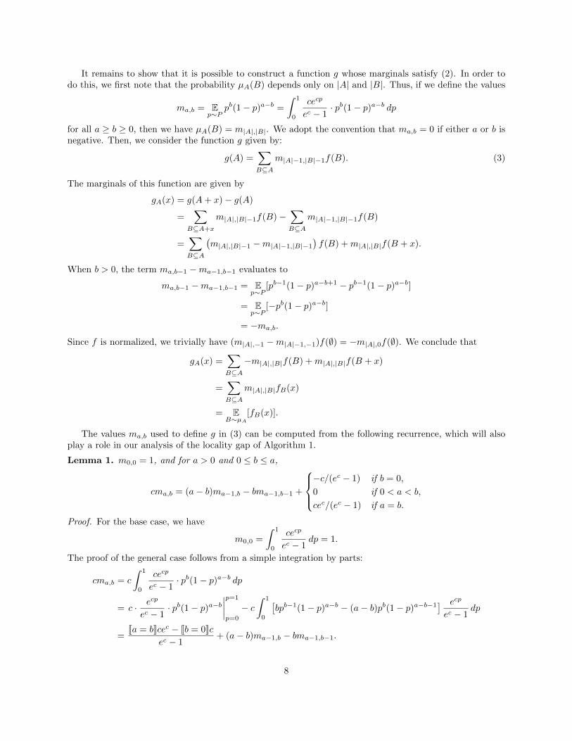
It remains to show that it is possible to construct a function g whose marginals satisfy (2). In order todo this, we first note that the probability µA(B) depends only on |A| and |B|. Thus, if we define the values

ma,b = Ep∼P

pb(1− p)a−b =

∫ 1

0

cecp

ec − 1· pb(1− p)a−b dp

for all a ≥ b ≥ 0, then we have µA(B) = m|A|,|B|. We adopt the convention that ma,b = 0 if either a or b isnegative. Then, we consider the function g given by:

g(A) =∑B⊆A

m|A|−1,|B|−1f(B). (3)

The marginals of this function are given by

gA(x) = g(A+ x)− g(A)

=∑

B⊆A+x

m|A|,|B|−1f(B)−∑B⊆A

m|A|−1,|B|−1f(B)

=∑B⊆A

(m|A|,|B|−1 −m|A|−1,|B|−1

)f(B) +m|A|,|B|f(B + x).

When b > 0, the term ma,b−1 −ma−1,b−1 evaluates to

ma,b−1 −ma−1,b−1 = Ep∼P

[pb−1(1− p)a−b+1 − pb−1(1− p)a−b]

= Ep∼P

[−pb(1− p)a−b]

= −ma,b.

Since f is normalized, we trivially have (m|A|,−1 −m|A|−1,−1)f(∅) = −m|A|,0f(∅). We conclude that

gA(x) =∑B⊆A

−m|A|,|B|f(B) +m|A|,|B|f(B + x)

=∑B⊆A

m|A|,|B|fB(x)

= EB∼µA

[fB(x)].

The values ma,b used to define g in (3) can be computed from the following recurrence, which will alsoplay a role in our analysis of the locality gap of Algorithm 1.

Lemma 1. m0,0 = 1, and for a > 0 and 0 ≤ b ≤ a,

cma,b = (a− b)ma−1,b − bma−1,b−1 +

−c/(ec − 1) if b = 0,

0 if 0 < a < b,

cec/(ec − 1) if a = b.

Proof. For the base case, we have

m0,0 =

∫ 1

0

cecp

ec − 1dp = 1.

The proof of the general case follows from a simple integration by parts:

cma,b = c

∫ 1

0

cecp

ec − 1· pb(1− p)a−b dp

= c · ecp

ec − 1· pb(1− p)a−b

∣∣∣∣p=1

p=0

− c∫ 1

0

[bpb−1(1− p)a−b − (a− b)pb(1− p)a−b−1

] ecp

ec − 1dp

=Ja = bKcec − Jb = 0Kc

ec − 1+ (a− b)ma−1,b − bma−1,b−1.

8

(When b = 0 the integrand simplifies to cecp

ec−1 · (1− p)a, and when a = b it simplifies to cecp

ec−1 · pb.)

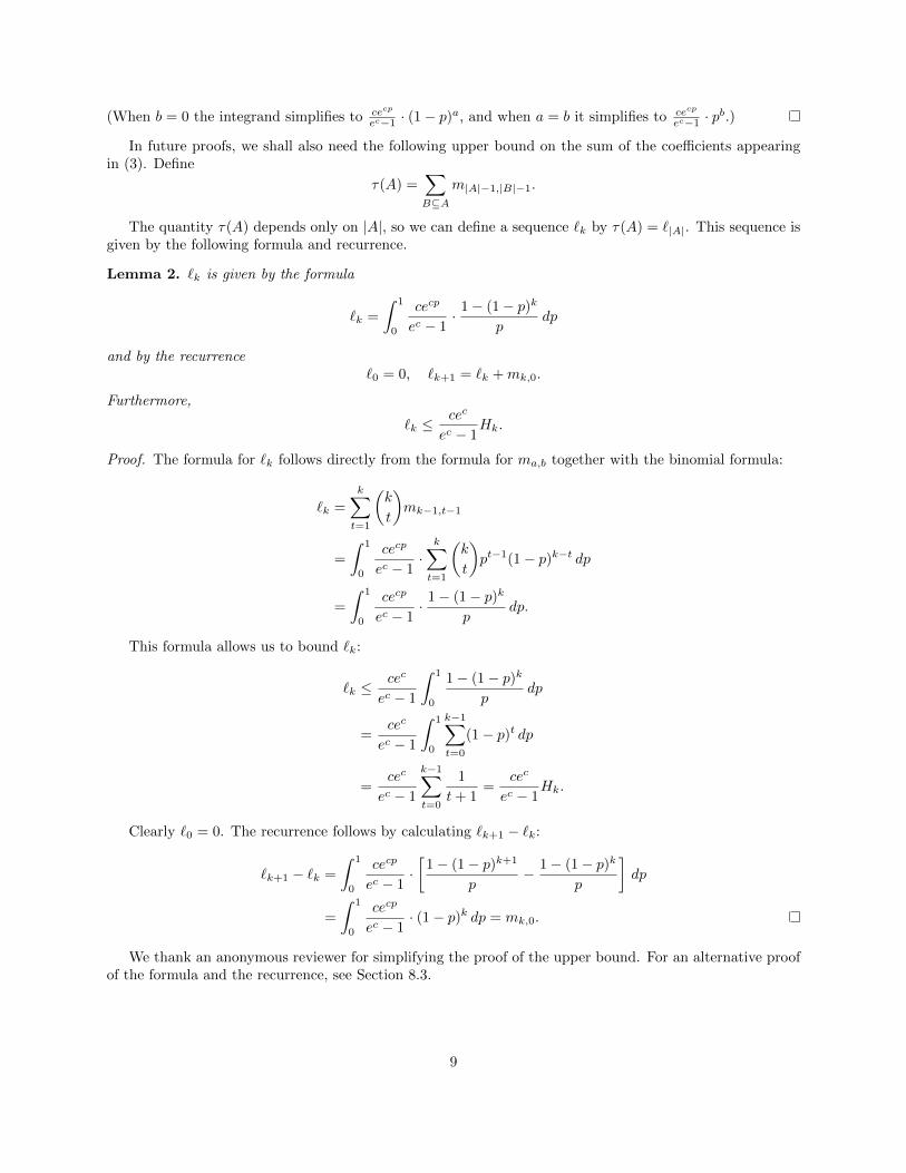
In future proofs, we shall also need the following upper bound on the sum of the coefficients appearingin (3). Define

τ(A) =∑B⊆A

m|A|−1,|B|−1.

The quantity τ(A) depends only on |A|, so we can define a sequence `k by τ(A) = `|A|. This sequence isgiven by the following formula and recurrence.

Lemma 2. `k is given by the formula

`k =

∫ 1

0

cecp

ec − 1· 1− (1− p)k

pdp

and by the recurrence`0 = 0, `k+1 = `k +mk,0.

Furthermore,

`k ≤cec

ec − 1Hk.

Proof. The formula for `k follows directly from the formula for ma,b together with the binomial formula:

`k =

k∑t=1

(k

t

)mk−1,t−1

=

∫ 1

0

cecp

ec − 1·k∑t=1

(k

t

)pt−1(1− p)k−t dp

=

∫ 1

0

cecp

ec − 1· 1− (1− p)k

pdp.

This formula allows us to bound `k:

`k ≤cec

ec − 1

∫ 1

0

1− (1− p)k

pdp

=cec

ec − 1

∫ 1

0

k−1∑t=0

(1− p)t dp

=cec

ec − 1

k−1∑t=0

1

t+ 1=

cec

ec − 1Hk.

Clearly `0 = 0. The recurrence follows by calculating `k+1 − `k:

`k+1 − `k =

∫ 1

0

cecp

ec − 1·[

1− (1− p)k+1

p− 1− (1− p)k

p

]dp

=

∫ 1

0

cecp

ec − 1· (1− p)k dp = mk,0.

We thank an anonymous reviewer for simplifying the proof of the upper bound. For an alternative proofof the formula and the recurrence, see Section 8.3.

9

4.2 Properties of g

We now show that our potential function g shares many basic properties with f .

Lemma 3. The function g is normalized, monotone, submodular and has curvature at most c.

Proof. From (3) we have g(∅) = m−1,−1f(∅) = 0. Thus, g is normalized. Additionally, (2) immediatelyimplies that g is monotone, since the monotonicity of f implies that each term fB(x) is non-negative. Next,suppose that A1 ⊆ A2 and x /∈ A2. Then from (2), we have

gA2(x) = EB∼µA2

fB(x) ≤ EB∼µA2

fB∩A1(x) = EB∼µA1

fB(x) = gA1(x),

where the inequality follows from submodularity of f . Thus, g is submodular. Finally, for any set A ⊆ Uand any element x /∈ A, we have

gA(x) = EB∼µA

fB(x) ≥ (1− c)f(x) = (1− c)g(x),

where the inequality follows from the bound on the curvature of f , and the second equality from settingA = ∅ in (2). Thus, g has curvature at most c. In fact, it is possible to show that for any given |A|, g has aslightly lower curvature than f , corresponding to our intuition that the distribution P blends together f andvarious functions of reduced curvature. For our purposes, however, an upper bound of c is sufficient.

Finally, we note that for any S ⊆ U , it is possible to bound the value g(S) relative to f(S).

Lemma 4. For any A ⊆ U ,f(A) ≤ g(A) ≤ cec

ec − 1H|A|f(A).

Proof. Let A = a1, . . . , a|A| and define Ai = a1, . . . , ai for 0 ≤ i ≤ |A|. The formula (2) implies that

gAi(ai+1) = EB∼µAi

fB(ai+1) ≥ fAi(ai+1).

Summing the resulting inequalities for i = 0 to |A| − 1, we get

g(A)− g(∅) ≥ f(A)− f(∅).

The lower bound then follows from the fact that both g and f are normalized, so g(∅) = f(∅) = 0.For the upper bound, (3) and monotonicity of f imply that

g(A) =∑B⊆A

m|A|−1,|B|−1f(B) ≤ f(A)∑B⊆A

m|A|−1,|B|−1.

The upper bound then follows directly from applying the bound of Lemma 2 to the final sum.

4.3 Approximating g via Sampling

Evaluating g(A) exactly requires evaluating f on all subsets B ⊆ A, and so we cannot compute g directlywithout using an exponential number of calls to the value oracle f . We now show that we can efficientlyestimate g(A) by using a sampling procedure that requires evaluating f on only a polynomial number ofsets B ⊆ A. In Section 7, we show how to use this sampling procedure to obtain a randomized variant ofAlgorithm 1 that runs in polynomial time.

We have already shown how to construct the function g, and how to interpret the marginals of g as theexpected value of a certain random experiment. Now we show that the direct definition of g(A) in (3) canalso be viewed as the result of a random experiment.

10

For a set A, consider the distribution νA on 2A given by

νA(B) =m|A|−1,|B|−1

τ(A).

Then, recalling the direct definition of g, we have:

g(A) =∑B⊆A

m|A|−1,|B|−1f(B) = τ(A) EB∼νA

[f(B)].

We can estimate g(A) to any desired accuracy by sampling from the distribution νA. This can be doneefficiently using the recurrences for ma,b and τ(A) given by Lemma 1 and Lemma 2, respectively. LetB1, . . . , BN be N independent random samples from νA. Then, we define:

g(A) = τ(A)1

N

N∑i=1

f(Bi). (4)

Lemma 5. Choose M, ε > 0, and set

N =1

2

(cec

ec − 1· Hn

ε

)2

lnM.

Then,Pr[|g(A)− g(S)| ≥ εg(S)] = O

(M−1

).

Proof. We use the following version of Hoeffding’s bound.

Fact (Hoeffding’s bound). Let X1, . . . , XN be i.i.d. non-negative random variables bounded by B, and let Xbe their average. Suppose that EX ≥ ρB. Then, for any ε > 0,

Pr[|X − EX| ≥ εEX] ≤ 2 exp(−2ε2ρ2N

).

Consider the random variables Xi = τ(A)f(Bi). Because f is monotone and each Bi is a subset of A,each Xi is bounded by τ(A)f(A). The average X of the values Xi satisfies

EX = g(A) ≥ f(A),

where the inequality follows from Lemma 4. Thus, Hoeffding’s bound implies that

Pr[|X − EX| ≥ εEX] ≤ 2 exp

(− 2ε2N

τ(A)2

).

By Lemma 2 we have τ(A) ≤ cec

ec−1H|A| ≤cec

ec−1Hn and so

2 exp

(− 2ε2N

τ(A)2

)≤ 2 exp (− lnM) = O

(M−1

).

5 Analysis of Algorithm 1

We now give a complete analysis of the runtime and approximation performance of Algorithm 1. Thealgorithm has two phases: a greedy phase and a local search phase. Both phases are guided by the auxiliarypotential function g defined in Section 4. As noted in Section 4.3, we cannot, in general, evaluate g inpolynomial time, though we can estimate g by sampling. However, sampling g complicates the algorithmand its analysis. We postpone such concerns until the next section, and in this section suppose that weare given a value oracle returning g(A) for any set A ⊆ U . We then show that Algorithm 1 requires only

11

a polynomial number of calls to the oracle for g. In this way, we can present the main ideas of the proofswithout a discussion of the additional parameters and proofs necessary for approximating g by sampling.In the next section we use the results of Lemma 5 to implement an approximate oracle for g in polynomialtime, and adapt the proofs given here to obtain a randomized, polynomial time algorithm.

Consider an arbitrary input to the algorithm. Let S = s1, . . . , sr be the solution returned by Algorithm1 on this instance and O be an optimal solution to this instance. It follows directly from the definition of thestandard greedy algorithm and the type of exchanges considered by Algorithm 1 that S is a base. Moreover,because f is monotone, we may assume without loss of generality that O is a base, as well. We index theelements oi of O by using the following lemma of Brualdi [4].

Fact (Brualdi’s lemma). Suppose A,B are two bases in a matroid. There is a bijection π : A→ B such thatfor all a ∈ A, A− a+ π(a) is a base. Furthermore, π is the identity on A ∩B.

The main difficulty in bounding the locality ratio of Algorithm 1 is that we must bound the ratiof(S)/f(O) stated in terms of f , by using only the fact that S is locally optimal with respect to g. Thus,we must somehow relate the values of f(S) and g(S). In the following theorem relates the values of f and gon arbitrary bases of a matroid. Later, we shall apply this theorem to S and O to obtain an approximationguarantee both for Algorithm 1 and for the randomized variant presented in the next section.

Theorem 1. Let A = a1, . . . , ar and B = b1, . . . , br be any two bases of M, and suppose f hascurvature at most c with respect to B. Further suppose that we index the elements of B so that bi = π(ai),where π : A→ B is the bijection guaranteed by Brualdi’s lemma. Then,

cec

ec − 1f(A) ≥ f(B) +

r∑i=1

[g(A)− g(A− ai + bi)].

Proof. First, we provide some general intuition for the proof. In order to prove the theorem, we fix a currentbase A of M and some other arbitrary base B, and consider each of the individual swaps from Brualdi’sLemma. Each such swap removes a single element of A and adds one element of B to the result. We considerthe change in g caused by each such swap. The value of g on any given set may be O(log n) times largerthan the corresponding value of f . Indeed, the value of g(A) is obtained by summing appropriately weightedvalues of f(A′) over all subsets A′ ⊆ A. However, we shall show that our definition of g ensures that when allthe differences g(A)−g(A−ai+bi) are added together, most of these values cancel. Specifically, cancellationbetween corresponding values f(A′) leave us with an expression in which all terms are bounded by f(A) orf(B). Specifically, we show that the sum of differences

∑ri=1[g(A)− g(A−ai+ bi)] reduces to a lower bound

on the difference between f(B) and cec

ec−1 f(A).Our proof involves two inequalities and one equation, each of which we shall prove later as a separate

lemma. The inequalities will pertain to the quantity

r∑i=1

gA−ai(ai), (5)

which represents (up to scaling) the average total loss in g(A) when a single element ai is removed from A.In Lemma 6, we use the basic definition and properties of g to show that the loss for each ai is bounded

by the difference g(A)− g(A− ai + bi) and a combination of marginal values of f . Then, by the linearity ofexpectation, we obtain

r∑i=1

gA−ai(ai) ≥r∑i=1

[g(A)− g(A− ai + bi)] + ET∼µA

r∑i=1

fT−bi(bi). (6)

In Lemma 7 (similar to Vondrak [35, Lemma 3.1]), we simplify the final term in (6), using the fact thatf has curvature at most c with respect to B. The lemma relates the sum of marginals fT−bi(bi) to f(T ),showing that

r∑i=1

fT−bi(bi) ≥ f(B)− cf(T ),

12

for any T ⊆ A and bi ∈ B. Applying the resulting inequalities in (6), we obtain the following bound on (5):

r∑i=1

gA−ai(ai) ≥r∑i=1

[g(A)− g(A− ai + bi)] + f(B)− c ET∼µA

f(T ). (7)

Finally, in Lemma 8 we reconsider (5), expanding the definition of g and adding the final term cET∼µA f(T )of (7) to the result. By exploiting the recurrence of Lemma 1, we show that all terms except those involvingf(A) vanish from the resulting expression. Specifically, we show the following equality involving (5):

r∑i=1

gA−ai(ai) + c ET∼µA

f(T ) =cec

ec − 1f(A). (8)

Combining the equality (8) with the lower bound on (5) from (7) then completes the proof.

We now prove each of the necessary lemmata.

Lemma 6. For all i ∈ [r],

gA−ai(ai) ≥ g(A)− g(A− ai + bi) + ET∼µA

fT−bi(bi).

Proof. The proof relies on the characterization of the marginals of g given in (2). We consider two cases:bi /∈ A and bi ∈ A. If bi /∈ A then the submodularity of g implies

gA−ai(ai) ≥ gA−ai+bi(ai)= g(A+ bi)− g(A− ai + bi)

= gA(bi) + g(A)− g(A− ai + bi)

= g(A)− g(A− ai + bi) + ET∼µA

fT (bi).

On the other hand, when bi ∈ A, we must have bi = π(ai) = ai by the definition of π. Then,

gA−ai(ai) = ET∼µA−ai

fT (ai)

= ET∼µA

fT−ai(ai)

= ET∼µA

fT−bi(bi)

= g(A)− g(A) + ET∼µA

fT−bi(bi)

= g(A)− g(A− ai + bi) + ET∼µA

fT−bi(bi),

where the second equality follows from the fact that if T ∼ µA then T ∩ (A \ ai) ∼ µA−ai .

Lemma 7. For any T ⊆ A,r∑i=1

fT−bi(bi) ≥ f(B)− cf(T ).

13

Proof. Our proof relies only on the submodularity and curvature of f . We have

r∑i=1

fT−bi(bi) =∑

bi∈B\T

fT (bi) +∑

bi∈B∩T

fT−bi(bi)

≥ f(T ∪B)− f(T ) +∑

bi∈B∩T

fT−bi(bi)

≥ f(T ∪B)− f(T ) +∑

bi∈B∩T

fT∪B−bi(bi)

≥ (1− c)f(T ) + f(B)− f(T )

= f(B)− cf(T )

where the first two inequalities follow from the submodularity of f and the last inequality from (1), since fhas curvature at most c with respect to B.

Lemma 8.r∑i=1

gA−ai(ai) + c ET∼µA

f(T ) =cec

ec − 1f(A). (9)

Proof. The proof relies primarily on the recurrence given in Lemma 1 for the values ma,b used to define g.From the characterization of the marginals of g given in (2) we have

gA−ai(ai) = ET∼µA−ai

[fT (ai)] = ET∼µA−ai

[f(T + ai)− f(T )].

Each subset D ⊆ A appears in the expectation. Specifically, if ai ∈ D then we have the term µA−ai(D −ai)f(D), and if ai ∈ A \D then we have the term −µA−ai(D)f(D). Therefore the coefficient of f(D) in theleft-hand side of (9) is thus given by(∑

ai∈DµA−ai(D − ai)

)−

(∑ai /∈D

µA−ai(D)

)+ cµA(D) = |D|mr−1,|D|−1 − (r − |D|)mr−1,|D| + cmr,|D|.

According to the recurrence for m, given in Lemma 1, the right-hand side vanishes unless D = ∅, in whichcase we get −c

ec−1f(∅) = 0, or D = A, in which case it is cec

ec−1f(A).

We are now ready to prove this section’s main claim, which gives bounds on both the approximationratio and complexity of Algorithm 1.

Theorem 2. Algorithm 1 is a(

1−e−cc − ε

)-approximation algorithm, requiring at most O(r2nε−1 log n)

evaluations of g.

Proof. We first consider the number of evaluations of g required by Algorithm 1. The initial greedy phaserequires O(rn) evaluations of g, as does each iteration of the local search phase. Thus, the total number ofevaluations of g required by Algorithm 1 is O(rnI), where I is the number of improvements applied in thelocal search phase. We now derive an upper bound on I.

Let g∗ = maxA∈I g(A) be the maximum value attained by g on any independent set in M. Algorithm 1begins by setting S to a greedy solution Sinit, and each time it selects an improved solution S′ to replace Sby, we must have

g(S′) > (1 + ε1)g(S)

Thus, the number of improvements that Algorithm 1 can apply is at most

log1+ε1

g∗

g(Sinit).

14

Fisher, Nemhauser, and Wolsey [20] show that the greedy algorithm is a 1/2-approximation algorithmfor maximizing any monotone submodular function subject to a matroid constraint. In particular, becauseg is monotone submodular, as shown in Lemma 3, we must have

I ≤ log1+ε1

g∗

g(Sinit)≤ log1+ε1 2 = O(ε−11 ) = O(rHrε

−1) = O(rε−1 log n).

Next, we consider the approximation ratio of Algorithm 1. Recall that O is an optimal solution of thearbitrary instance (M = (U , I), f) on which Algorithm 1 returns the solution S. We apply Theorem 1 tothe bases S and O, indexing S and O as in the theorem so that S − si + oi ∈ I for all i ∈ [r], to obtain:

cec

ec − 1f(S) ≥ f(O) +

r∑i=1

[g(S)− g(S − si + oi).] (10)

Then, we note that we must haveg(S − si + oi) ≤ (1 + ε1)g(S)

for each value i ∈ [r]—otherwise, Algorithm 1 would have exchanged si for oi rather than returning S.Summing the resulting r inequalities gives

r∑i=1

[g(S)− g(S − si + oi)] ≥ −rε1g(S).

Applying this and upper bound on g(S) from Lemma 4 to (10) we then obtain

cec

ec − 1f(S) ≥ f(O)− rε1g(S) ≥ f(O)− cec

ec − 1rε1Hrf(S) ≥ f(O)− cec

ec − 1rε1Hrf(O).

Rewriting this inequality using the definition ε1 = εrHr

then gives

f(S) ≥(

1− e−c

c− ε)f(O),

and so Algorithm 1 is a(

1−e−cc − ε

)-approximation algorithm.

6 How g was Constructed

The definition of our potential function g might seem somewhat mysterious. In this section we try to dispelsome of this mystery. First, we explain how we initially found the definition of g by solving a sequenceof factor-revealing linear programs. Second, we show how the definition of g follows directly from requiredproperties in the proof of our main technical result, Theorem 1.

6.1 Factor-revealing LP

The main idea behind our construction of the function g was to consider a general class of possible functions,and then optimize over this class of functions. We consider a mathematical program whose variables aregiven by the values defining a submodular function f and the parameters defining a related potential functiong, and whose objective function is the resulting locality gap for the instance defined by f . This technique ofusing a factor-revealing LP, which gives the approximation ratio of some algorithm over a particular familyof instances, appears formally in Jain et al. [25] in the context of greedy facility location algorithms, buthad been applied earlier by Goemans and Kleinberg [23] to analyze an algorithm for the minimum latencyproblem. Here, however, we use the linear program not only to find the best possible approximation ratiofor our approach, but also to determine the potential function g that yields this ratio.

15

The class of functions that we consider are functions of the form

g(A) =∑B⊆A

G|A|,|B|f(A). (11)

Since we assume that f is normalized, we can take Ga,b = 0 when b = 0. Our local search algorithm onlyevaluates g at sets whose size are the rank r of the matroid, so we can assume that |A| = r. (The greedyphase evaluates g at sets of smaller size, but as we explain in Section 3, this phase can be replaced by phasesnot evaluating g at all.) The optimal choice of coefficients Gr,k, and the resulting approximation ratio, aregiven by the following program Π:

maxGr,1,...,Gr,r

minf

f(S)

f(O)

s.t.

g(S) ≥ g(S − si + oi) for i ∈ [r]

f is normalized and monotone submodular, and has curvature c with respect to O

Given the values of Gr,1, . . . , Gr,r, the inner program (the part starting with minf f(S)/f(O)) evaluatesthe approximation ratio of the resulting local search algorithm, assuming that the optimal set O and theset produced by the algorithm S are disjoint (the analysis of Algorithm 1 will have to show that the sameapproximation ratio is obtained even when O and S are not disjoint). The variables of the inner programare the 22r values of the function f on all subsets of S ∪ O, where S = s1, . . . , sr and O = o1, . . . , orare two fixed disjoint sets of cardinality r. The constraints g(S) ≥ g(S − si + oi) state that the set S islocally optimal with respect to the function g (implicitly relying on Brualdi’s lemma). These constraints areexpanded into linear constraints over the variables of the program by substituting the definition of g givenby (11).

The program Π is equivalent to a linear program. In order to convert Π into a linear program, wefirst add an additional constraint f(O) = 1, thus making the inner program a linear program. We thendualize the inner program and obtain a linear program with a maximized objective function. Folding bothmaximization operators, we obtain a linear program Π′ whose value is the same as the value of Π. Sincethe inner program in Π has exponentially many variables, the linear program Π′ has exponentially manyconstraints. Symmetry considerations allow us to reduce the number of variables in the inner program toO(r3), obtaining an equivalent polynomial-size linear program Π′′ which can be solved in polynomial time.See Ward [37, §4.3] for more details.

We have implemented the linear program Π′′ on a computer, and calculated the coefficients Gr,1, . . . , Gr,rand the resulting approximation ratio for various values of r and c. The resulting approximation ratios areslightly larger than (1 − e−c)/c, but as r becomes bigger, the approximation ratio approaches (1 − e−c)/c.The function g considered in this paper is obtained by (in some sense) taking the limit r →∞.3

3In the case of maximum coverage, discussed in Section 8.3, the idea of taking the limit r → ∞ can be explained formally.The general form of the function g in that case is

g(A) =∑x∈V

`|A[x]|w(x),

where V is the universe of elements, w : V → R≥0 is the weight function, A[x] is the subset of A consisting of all sets containingx, and (`t)t∈N are the coefficients determining the function g. For each rank r, one can construct a linear program Πr involving`0, . . . , `r that determines the best choice of coefficients. See Ward [37, §3.4] for more details (there the sequence is known as(αt)t∈N). For r1 ≤ r2, the linear program Πr1 is obtained from Πr2 by removing all constraints involving `t for t > r1. Wecan thus construct an infinite linear program Π∞ in infinitely many variables (`t)t∈N which extends all linear programs Πr.The program Π∞ has the value 1 − 1/e, attained by the unique choice of coefficients detailed in Section 8.3. This leads to alimiting function gMC in the case of maximum coverage. The function g considered in this paper is the unique function of theform (11) which reduces to gMC when f is a coverage function.

16

6.2 Proof Analysis

Another approach to understanding our choice of g is by analyzing the proof of the locality ratio of Algo-rithm 1, given by Theorem 1:

cec

ec − 1f(S) ≥ f(O) +

r∑i=1

[g(S)− g(S − si + oi)].

Here O = o1, . . . , or is a global optimum of f (over the matroid), S = s1, . . . , sr, and the indices arechosen so that S − si + oi ∈ I (using Brualdi’s lemma). The locality ratio is the minimal possible valueof f(S)/f(O) over all locally optimal S (sets for which g(S) ≥ g(S − si + oi) for all i ∈ [r]), in this case(1− e−c)/c.

The analysis of Algorithm 1 relies on the fact that g satisfies (2) for some coefficients µA(B):

gA(x) =∑B⊆A

µA(B)fB(x). (2)

We suppose that the value of g is invariant under permutations of the ground set U . It immediately followsthat µA(B) should depend only on |A|, |B| and hence, also be invariant under permutations of U . We obtainmore constraints on µA(B) by examining the proof of the submodularity of g in Lemma 3: if A1 ⊆ A2 then

gA2(x) =

∑B⊆A2

µA2(B)fB(x)

(∗)≤

∑B⊆A2

µA2(B)fB∩A1

(x)(†)=∑B⊆A1

µA1(B)fB(x) = gA1

(x).

Inequality (∗) requires µA2(B) ≥ 0, while (†) implies4 that∑

B2⊆A2B2∩A1=B1

µA2(B2) = µA1(B1). (12)

Summing this over all B1 ⊆ A1, we deduce∑B2⊆A2

µA2(B2) =

∑B1⊆A1

µA1(B1).

Without loss of generality, we can assume that the common value of this sum is 1. Since µA2(B) ≥ 0, we canthus regard µA2 as a probability distribution over subsets of A. Equation (12) then states that if X ∼ µA2

then X ∩A1 ∼ µA1.

We now show that this restriction property of the distributions µA allows us to recover µA up to thespecific distribution P used in the definition g. Suppose that the ground set U were infinite, say U = N.For each n ∈ N, µ[n] is a distribution over subsets of [n]. We can define a single distribution µ over subsetsof N by the following rule: if X ∼ µ then for all n ∈ N, X ∩ [n] ∼ µ[n]. Note that because each µ[n]

satisfies the restriction property, the distribution µ is indeed well-defined. We can think of µ as a collectionof indicator random variables (Xi)i∈N encoding the chosen subset. Although the random variables Xi arenot independent, we note they are exchangeable — because µA(B) is invariant under permutations of U ,(Xi)i∈N has the same distribution as (Xπ(i))i∈N for all permutations π on N — and so de Finetti’s theoremimplies that there exists a probability distribution P supported on [0, 1] such that

µA(B) = Ep∈P

p|B|(1− p)|A|−|B|.

As in Section 4.1, we can then define the values ma,b = Ep∈P pb(1− p)a−b, and let g be given by

g(A) =∑B⊆A

m|A|−1,|B|−1f(B). (3)

4In order to deduce submodularity, we in fact only need (†) to hold as an inequality; but for the submodularity of g to be“tight”, equality is required.

17

It remains to deduce the exact distribution P . In order to do this, we consider the other property of gused in the proof of Theorem 1, namely Lemma 1. The general form of this lemma is

cma,b = (a− b)ma−1,b − bma−1,b−1 +

C0 if b = 0,

0 if 0 < a < b,

C1 if a = b.

The locality ratio proved in Theorem 1 is 1/C1, and the proof requires C0 ≤ 0. Lemma 1 is proved usingintegration by parts. Let F ′(p) be the density of P , and let F (p) be an antiderivative of F ′(p) (not necessarilythe cumulative distribution function of P ). We can then restate the proof of Lemma 1 as follows:

cma,b = c

∫ 1

0

F ′(p) · pb(1− p)a−b dp

= cF (p) · pb(1− p)a−b∣∣p=1

p=0− c

∫ 1

0

F (p) · [bpb−1(1− p)a−b − (a− b)pb(1− p)a−b−1] dp

(‡)= Ja = bKcF (1)− Jb = 0KcF (0) + (a− b)ma−1,b − bma−1,b−1.

In order for equation (‡) to hold, F must satisfy the differential equation F ′ = cF whose solution is F (p) ∝ecp. Since P is a probability distribution supported on [0, 1], we must have F (1) − F (0) = 1 and soF (p) = ecp/(ec − 1). We deduce that F ′(p) = cecp/(ec − 1), and that the locality ratio is 1/(cF (1)) =1/F ′(1) = (1− e−c)/c.

7 A randomized, polynomial-time algorithm

Our analysis of Algorithm 1 supposed that we were given an oracle for computing the value of the potentialfunction g. We now use the results of Lemma 5, which shows that the value g(A) can be approximated for anyA by using a polynomial number of samples, to implement a randomized, polynomial-time approximationalgorithm that does not require an oracle for g. The resulting algorithm attains the same approximationratio as Algorithm 1 with high probability. The analysis of the modified algorithm, while somewhat tedious,is standard and in the spirit of earlier results such as Calinescu at al. [8].

The modified algorithm is shown in Algorithm 2. Algorithm 2 uses an approximation g of g that isobtained by taking N independent random samples of f each time g is calculated. The number of samplesN depends on the parameters ε and α, in addition to the rank r of M the size n of U . As in Algorithm1, ε governs how much an exchange must improve the current solution before it is applied, and so affectsboth the approximation performance and runtime of the algorithm. The additional parameter α controls

the probability that Algorithm 2 fails to produce a(

1−e−cc − ε

)-approximate solution. Specifically, we show

that Algorithm 2 fails with probability at most O(n−α).For the analysis, we assume that ε ≤ 1 and r ≥ 2, which imply that ε2 ≤ 1/12.The local search routine in Algorithm 2 runs some number I of iterations, signaling an error if it fails

to converge to a local optimum after this many improvements. In each iteration, the algorithm searchesthrough all possible solutions S′ = S − x + y, sampling the value g(S′) if S′ ∈ I. If the sampled value ofg(S′) exceeds the sampled value for g(S) by a factor of at least (1 + ε2), the algorithm updates S and movesto the next iteration. Otherwise, it returns the current solution. Note that we store the last sampled valueg(S) of the current solution in v, rather than resampling g(S) each time we check an improvement S′.

The analysis of Algorithm 2 follows the same general pattern as that presented in the previous section.Here however, we must address the fact that g does not always agree with g. First, we estimate the probabilitythat all of the computations of g made by Algorithm 2 are reasonably close to the value of g.

Lemma 9. With probability 1−O(n−α), we have |g(A)− g(A)| ≤ ε2g(A) for all sets A for which Algorithm2 computes g(A).

18

Input: M = (U , I), f, c, ε, αSet ε2 = ε

4rHr

Set I =((

1+ε21−ε2

)(2 + 3rε2)− 1

)ε−12

Set N = 12

(cec

ec−1 ·Hnε2

)2ln((I + 1)rn1+α

)Let g be an approximation to g computed by taking N random samplesLet Sinit be the result of running the standard greedy algorithm on (M, g)S ← Sinit

v ← g(Sinit)for i← 1 to I do Search for at most I iterations

done← trueforeach element x ∈ S and y ∈ U \ S do

S′ ← S − x+ yif S′ ∈ I then

v′ ← g(S′)if v′ > (1 + ε2)v then An improved solution S′ was found

v ← v′ and S ← S′ update v and Sdone← falsebreak and continue to the next iteration

if done then return S No improvement was found, return local optimumreturn Error (Search did not converge in I iterations)

Algorithm 2: The non-oblivious local search algorithm

Proof. We first bound the total number of sets A for which Algorithm 2 computes g(A). The initial greedyphase requires fewer than rn evaluations, as does each of the I iterations of the local phase. The totalnumber of evaluations is therefore less than (I + 1)rn.

Algorithm 2 uses

N =1

2

(cec

ec − 1· Hn

ε2

)2

ln((I + 1)rn1+α

)samples for every computation of g(A). By Lemma 5, the probability that we have |g(A)− g(A)| ≥ ε2g(A)

for any given set A is then δ = O(

1(I+1)rn1+α

).

Let the sets at which Algorithm 2 evaluates g be A1, . . . , AM , where M ≤ (I+1)rn; both M and the setsAi are random variables depending on the execution of the algorithm. The events |g(Ai)− g(Ai)| ≥ ε2g(Ai)are independent, and so from the union bound, the probability that at least one of the sets Ai does not

satisfy the desired error bound is at most O(

(I+1)rn(I+1)rn1+α

)= O(n−α).

We call the condition that |g(A)− g(A)| ≤ ε2g(A) for all sets A considered by Algorithm 2 the samplingassumption. Lemma 9 shows that the sampling assumption holds with high probability.

Now, we must adapt the analysis of Section 5, which holds when g is computed exactly, to the setting inwhich g is computed approximately. In Theorem 2, we showed that g(Sinit) is within a constant factor ofthe largest possible value that g could take on any set A ⊆ U . Then, because the algorithm always improvedg by a factor of at least (1 + ε1), we could bound the number of local search iterations that it performed.Finally, we applied Theorem 1 to translate the local optimality of S with respect to g into a lower bound onf(S).

Here we follow the same general approach. First, we derive the following result, which shows that theinitial value g(Sinit) is within a constant factor of the maximum value g∗ of g(A) on any set A considered

19

by Algorithm 2.5

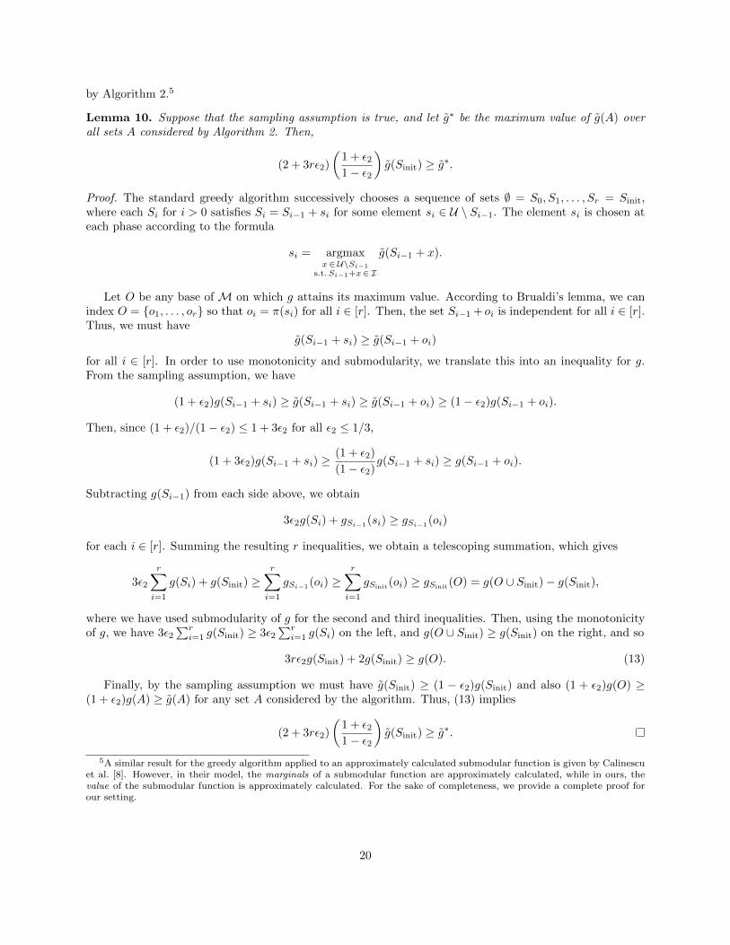
Lemma 10. Suppose that the sampling assumption is true, and let g∗ be the maximum value of g(A) overall sets A considered by Algorithm 2. Then,

(2 + 3rε2)

(1 + ε21− ε2

)g(Sinit) ≥ g∗.

Proof. The standard greedy algorithm successively chooses a sequence of sets ∅ = S0, S1, . . . , Sr = Sinit,where each Si for i > 0 satisfies Si = Si−1 + si for some element si ∈ U \ Si−1. The element si is chosen ateach phase according to the formula

si = argmaxx∈U\Si−1

s.t.Si−1+x∈I

g(Si−1 + x).

Let O be any base of M on which g attains its maximum value. According to Brualdi’s lemma, we canindex O = o1, . . . , or so that oi = π(si) for all i ∈ [r]. Then, the set Si−1 + oi is independent for all i ∈ [r].Thus, we must have

g(Si−1 + si) ≥ g(Si−1 + oi)

for all i ∈ [r]. In order to use monotonicity and submodularity, we translate this into an inequality for g.From the sampling assumption, we have

(1 + ε2)g(Si−1 + si) ≥ g(Si−1 + si) ≥ g(Si−1 + oi) ≥ (1− ε2)g(Si−1 + oi).

Then, since (1 + ε2)/(1− ε2) ≤ 1 + 3ε2 for all ε2 ≤ 1/3,

(1 + 3ε2)g(Si−1 + si) ≥(1 + ε2)

(1− ε2)g(Si−1 + si) ≥ g(Si−1 + oi).

Subtracting g(Si−1) from each side above, we obtain

3ε2g(Si) + gSi−1(si) ≥ gSi−1(oi)

for each i ∈ [r]. Summing the resulting r inequalities, we obtain a telescoping summation, which gives

3ε2

r∑i=1

g(Si) + g(Sinit) ≥r∑i=1

gSi−1(oi) ≥

r∑i=1

gSinit(oi) ≥ gSinit

(O) = g(O ∪ Sinit)− g(Sinit),

where we have used submodularity of g for the second and third inequalities. Then, using the monotonicityof g, we have 3ε2

∑ri=1 g(Sinit) ≥ 3ε2

∑ri=1 g(Si) on the left, and g(O ∪ Sinit) ≥ g(Sinit) on the right, and so

3rε2g(Sinit) + 2g(Sinit) ≥ g(O). (13)

Finally, by the sampling assumption we must have g(Sinit) ≥ (1 − ε2)g(Sinit) and also (1 + ε2)g(O) ≥(1 + ε2)g(A) ≥ g(A) for any set A considered by the algorithm. Thus, (13) implies

(2 + 3rε2)

(1 + ε21− ε2

)g(Sinit) ≥ g∗.

5A similar result for the greedy algorithm applied to an approximately calculated submodular function is given by Calinescuet al. [8]. However, in their model, the marginals of a submodular function are approximately calculated, while in ours, thevalue of the submodular function is approximately calculated. For the sake of completeness, we provide a complete proof forour setting.

20

The next difficulty we must overcome is that the final set S produced by Algorithm 2 is (approximately)locally optimal only with respect to the sampled function g(S). In order to use Theorem 1 to obtain alower bound on f(S), we must show that S is approximately locally optimal with respect to g as well. Weaccomplish this in our next lemma, by showing that any significant improvement in g must correspond to a(somewhat less) significant improvement in g.

Lemma 11. Suppose that the sampling assumption holds and that g(A) ≤ (1+ ε2)g(B) for some pair of setsA,B considered by Algorithm 2. Then

g(A) ≤ (1 + 4ε2)g(B)

Proof. From the sampling assumption, we have

(1− ε2)g(A) ≤ g(A) ≤ (1 + ε2)g(B) ≤ (1 + ε2)(1 + ε2)g(B).

Thus

g(A) ≤ (1 + ε2)2

1− ε2g(B) ≤ (1 + 4ε2)g(B),

where the second inequality holds since ε2 ≤ 1/5.

We now prove our main result.

Theorem 3. Algorithm 2 runs in time O(r4nε−3α) and returns a(

1−e−cc − ε

)-approximation with proba-

bility 1−O(n−α).

Proof. As in the proof of Theorem 2, we consider some arbitrary instance (M = (U , I), f) of monotonesubmodular matroid maximization with upper bound c on the curvature of f , and let O be an optimalsolution of this instance. We shall show that if the sampling assumption holds, Algorithm 2 returns a solution

S satisfying f(S) ≥(

1−e−cc − ε

)f(O). Lemma 9 shows that this happens with probability 1−O(n−α).

As in Algorithm 2, set

I =

((1 + ε21− ε2

)(2 + 3rε2)− 1

)ε−12 .

Suppose that the sampling assumption holds, and let g∗ be the maximum value taken by g(A) for any setA considered by Algorithm 2. At each iteration of Algorithm 2, either a set S is returned, or the value v isincreased by a factor of at least (1+ ε2). Suppose that the local search phase of Algorithm 2 fails to convergeto a local optimum after I steps, and so does not return a solution S. Then we must have

v ≥ (1 + ε2)I g(Sinit) > (1 + Iε2)g(Sinit) =

(1 + ε21− ε2

)(2 + 3rε2)g(Sinit) ≥ g∗,

where the last inequality follows from Lemma 10. But, then we must have g(A) > g∗ for some set Aconsidered by the algorithm. Thus Algorithm 2 must produce a solution S.

As in Theorem 2, we apply Theorem 1 to the bases S and O, indexing S and O as in the theorem so thatS − si + oi ∈ I for all i ∈ [r], to obtain:

cec

ec − 1f(S) ≥ f(O) +

r∑i=1

[g(S)− g(S − si + oi).] (14)

Then, since Algorithm 2 returned S, we must then have:

g(S − si + oi) ≤ (1 + ε2)g(S)

for all i ∈ [r]. From Lemma 11 we then have

g(S − si + oi) ≤ (1 + 4ε2)g(S)

21

for all i ∈ [r]. Summing the resulting r inequalities gives

r∑i=1

[g(S)− g(S − si + oi)] ≥ −4rε2g(S).

Applying Theorem 2 and the upper bound on g(S) from Lemma 4 in (14), we then have

cec

ec − 1f(S) ≥ f(O)− 4rε2g(S) ≥ f(O)− cec

ec − 14rε2Hrf(S) ≥ f(O)− cec

ec − 14rε2Hrf(O).

Rewriting this inequality using the definition ε2 = ε4rHr

then gives

f(S) ≥(

1− e−c

c− ε)f(O).

The running time of Algorithm 2 is dominated by the number of calls it makes to the value oracle for f .We note, as in the proof of Lemma 9, that the algorithm evaluates g(A) on O(rnI) sets A. Each evaluationrequires N samples of f , and so the resulting algorithm requires

O(rnIN) = O(rnε−32 α) = O(r4nε−3α)

calls to the value oracle for f .

8 Extensions

The algorithm presented in Section 3 produces a (1− e−c)/c− ε approximation for any ε > 0, and it requiresknowledge of c. In this section we show how to produce a clean (1 − e−c)/c approximation, and how todispense with the knowledge of c. Unfortunately, we are unable to combine both improvements for technicalreasons.

It will be useful to define the function

ρ(c) =1− e−c

c,

which gives the optimal approximation ratio.

8.1 Clean approximation

In this section, we assume c is known, and our goal is to obtain a ρ(c) approximation algorithm. Weaccomplish this by combining the algorithm from Section 7 with partial enumeration.

For x ∈ U we consider the contracted matroid M/x on U − x whose independent sets are given byIx = A ⊆ U −x : A+x ∈ I, and the contracted submodular function (f/x) which is given by (f/x)(A) =f(A + x). It is easy to show that this function is a monotone submodular function whenever f is, and hascurvature at most that of f . Then, for each x ∈ U , we apply Algorithm 2 to the instance (M/x, f/x) toobtain a solution Sx. We then return Sx + x for the element x ∈ U maximizing f(Sx + x).

Fisher, Nemhauser, and Wolsey [31] analyze this technique in the case of submodular maximization over auniform matroid, and Khuller, Moss, and Naor [27] make use of the same technique in the restricted settingof budgeted maximum coverage. Calinescu et al. [7] use a similar technique to eliminate the error termfrom the approximation ratio of the continuous greedy algorithm for general monotone submodular matroidmaximization. Our proof relies on the following general claim.

Lemma 12. Suppose A ⊆ O and B ⊆ U \A satisfy f(A) ≥ (1− θA)f(O) and fA(B) ≥ (1− θB)fA(O \A).Then

f(A ∪B) ≥ (1− θAθB)f(O).

22

Proof. We have

f(A ∪B) = fA(B) + f(A)

≥ (1− θB)fA(O \A) + f(A)

= (1− θB)f(O) + θBf(A)

≥ (1− θB)f(O) + θB(1− θA)f(O)

= (1− θAθB)f(O).

Using Lemma 12 we show that the partial enumeration procedure gives a clean ρ(c)-approximationalgorithm.

Theorem 4. The partial enumeration algorithm runs in time O(r7n2α), and with probability 1 − O(n−α),the algorithm has an approximation ratio of ρ(c).

Proof. Let O = o1, . . . , or be an optimal solution to some instance (M, f). Since the submodularity of fimplies

r∑i=1

f(oi) ≥ f(O),

there is some x ∈ O such that f(x) ≥ f(O)/r. Take A = x and B = Sx in Lemma 12. Then, from Theorem3 we have (f/x)(Sx) ≥ (ρ(c)− ε)f(O) with probability 1−O(n−α) for any ε. We set ε = (1−ρ(c))/r. Then,substituting θA = 1−1/r and θB = 1−ρ(c) + (1−ρ(c))/r, we deduce that the resulting approximation ratioin this case is

1−(

1− 1

r

)(1− ρ(c) +

1− ρ(c)

r

)= 1−

(1− 1

r

)(1 +

1

r

)(1− ρ(c))

≥ 1− (1− ρ(c)) = ρ(c).

The partial enumeration algorithm simply runs Algorithm 2 n times, using ε = O(r−1) and so its runningtime is O(r7n2α).

8.2 Unknown curvature

In this section, we remove the assumption that c is known, but retain the error parameter ε. The keyobservation is that if a function has curvature c then it also has curvature c′ for any c′ ≥ c. This, combinedwith the continuity of ρ, allows us to “guess” an approximate value of c.

Given ε, consider the following algorithm. Define the set C of curvature approximations by

C = kε : 1 ≤ k ≤ bε−1c ∪ 1.

For each guess c′ ∈ C, we run the main algorithm with that setting of c′ and error parameter ε/2 to obtaina solution Sc′ . Finally, we output the set Sc′ maximizing f(Sc′).

Theorem 5. Suppose f has curvature c. The unknown curvature algorithm runs in time O(r4nε−4α), andwith probability 1−O(n−α), the algorithm has an approximation ratio of ρ(c)− ε.

Proof. From the definition of C it is clear that there is some c′ ∈ C satisfying c ≤ c′ ≤ c + ε. Since fhas curvature c, the set Sc′ is a ρ(c′) − ε/2 approximation. Elementary calculus shows that on (0, 1], thederivative of ρ is at least −1/2, and so we have

ρ(c′)− ε/2 ≥ ρ(c+ ε)− ε/2 ≥ ρ(c)− ε/2− ε/2 = ρ(c)− ε.

23

8.3 Maximum Coverage

In the special case that f is given explicitly as a coverage function function, we can evaluate the potentialfunction g exactly in polynomial time. A (weighted) coverage function is a particular kind of monotonesubmodular function that may be given in the following way. There is a universe V with non-negative weightfunction w : V → R≥0. The weight function is extended to subsets of V linearly, by letting w(S) =

∑s∈S w(s)

for all S ⊆ V. Additionally, we are given a family Vaa∈U of subsets of V, indexed by a set U . The functionf is then defined over the index set U , and f(A) is simply the total weight of all elements of V that arecovered by those sets whose indices appear in A. That is, f(A) = w

(⋃a∈A Va

).

We now show how to compute the potential function g exactly in this case. For a set A ⊆ U and anelement x ∈ V, we denote by A[x] the collection a ∈ A : x ∈ Va of indices a such that x is in the set Va.Then, recalling the definition of g(A) given in (3), we have

g(A) =∑B⊆A

m|A|−1,|B|−1f(B)

=∑B⊆A

m|A|−1,|B|−1∑

x∈⋃b∈B Vb

w(x)

=∑x∈V

w(x)∑

B⊆A s.t.A[x]∩B 6=∅

m|A|−1,|B|−1.

Consider the coefficient of w(x) in the above expression for g(A). We have∑B⊆A s.t.A[x]∩B 6=∅

m|A|−1,|B|−1 =∑B⊆A

m|A|−1,|B|−1 −∑

B⊆A\A[x]

m|A|−1,|B|−1

=

|A|∑i=0

(|A|i

)m|A|−1,i−1 −

|A\A[x]|∑i=0

(|A \A[x]|

i

)m|A|−1,i−1

=

|A|∑i=0

(|A|i

)Ep∼P

[pi−1(1− p)|A|−i] −|A\A[x]|∑i=0

(|A \A[x]|

i

)Ep∼P

[pi−1(1− p)|A|−i]

= Ep∼P

1

p

|A|∑i=0

(|A|i

)pi(1− p)|A|−i − (1− p)|A[x]|

p

|A\A[x]|∑i=1

(|A \A[x]|

i

)pi(1− p)|A\A[x]|−i

= Ep∼P

[1− (1− p)|A[x]|

p

].

Thus, if we define

`k = Ep∼P

[1− (1− p)k

p

]we have

g(A) =∑x∈V

`|A[x]|w(x),

and so to compute g, it is sufficient to maintain for each element x ∈ V a count of the number of sets A[x]with indices in A that contain x. Using this approach, each change in g(S) resulting from adding an elementx to S and removing an element e from S during one step of the local search phase of Algorithm 1 can becomputed in time O(|V|).

We further note that the coefficients `k are easily calculated using the following recurrence. For k = 0,

`0 = Ep∼P

[1− (1− p)0

p

]= 0,

24

while for k > 0,

`k+1 = Ep∼P

[1− (1− p)k+1

p

]= Ep∼P

[1− (1− p)k + p(1− p)k

p

]= `k + E

p∼P(1− p)k = `k +mk,0.

The coefficients `k obtained in this fashion in fact correspond (up to a constant scaling factor) to those usedto define the non-oblivious coverage potential in [17], showing that our algorithm for monotone submodularmatroid maximization is indeed a generalization of the algorithm already obtained in the coverage case.

When all subsets Va consist of the same element Va = x of weight w(x) = 1,

g(A) =∑B⊆A

m|A|−1,|B|−1f(B) =∑

B⊆A s.t.B 6=∅

m|A|−1,|B|−1 = τ(A).

(The quantity τ(A) is defined in Section 4.1.) On the other hand, g(A) = `|A|. We conclude that τ(A) = `|A|.

References

[1] Alexander A. Ageev and Maxim I. Sviridenko. Pipage rounding: A new method of constructing algo-rithms with proven performance guarantee. J. of Combinatorial Optimization, 8(3):307–328, September2004.

[2] Paola Alimonti. New local search approximation techniques for maximum generalized satisfiabilityproblems. In CIAC: Proc. of the 2nd Italian Conf. on Algorithms and Complexity, pages 40–53, 1994.

[3] B. V. Ashwinkumar and Jan Vondrak. Fast algorithms for maximizing submodular functions. InProceedings of the 25th annual ACM–SIAM Symposium on Discrete Algorithms (SODA), 2014.

[4] Richard A. Brualdi. Comments on bases in dependence structures. Bull. of the Austral. Math. Soc.,1(02):161–167, 1969.

[5] Niv Buchbinder, Moran Feldman, Joseph (Seffi) Naor, and Roy Schwartz. A tight linear time (1/2)-approximation for unconstrained submodular maximization. In FOCS, 2012.

[6] Niv Buchbinder, Moran Feldman, Joseph (Seffi) Naor, and Roy Schwartz. Submodular maximizationwith cardinality constraints. In Proceedings of the 25th annual ACM–SIAM Symposium on DiscreteAlgorithms (SODA), 2014.

[7] Gruia Calinescu, Chandra Chekuri, Martin Pal, and Jan Vondrak. Maximizing a submodular setfunction subject to a matroid constraint (Extended abstract). In IPCO, pages 182–196, 2007.

[8] Gruia Calinescu, Chandra Chekuri, Martin Pal, and Jan Vondrak. Maximizing a monotone submodularfunction subject to a matroid constraint. SIAM J. Comput., 40(6):1740–1766, 2011.

[9] Chandra Checkuri, Jan Vondrak, and Rico Zenklusen. Submodular function maximization via themultilinear relaxation and contention resolution schemes. In STOC, 2011.

[10] Chandra Chekuri, Jan Vondrak, and Rico Zenklusen. Dependent randomized rounding via exchangeproperties of combinatorial structures. Proceedings of the 2010 IEEE 51st Annual Symposium on Foun-dations of Computer Science, pages 575–584, 2010.

[11] Jack Edmonds. Matroids and the greedy algorithm. Math. Programming, 1(1):127–136, 1971.

[12] Uriel Feige. A threshold of ln n for approximating set cover. J. ACM, 45:634–652, July 1998.

[13] Uriel Feige, Vahab S. Mirrokni, and Jan Vondrak. Maximizing non-monotone submodular functions. InFOCS, pages 461–471, 2007.

25

[14] Moran Feldman, Joseph Naor, and Roy Schwartz. A unified continuous greedy algorithm for submodularmaximization. In FOCS, pages 570–579, 2011.

[15] Moran Feldman, Joseph (Seffi) Naor, and Roy Schwartz. Nonmonotone submodular maximization viaa structural continuous greedy algorithm. In ICALP, pages 342–353, 2011.

[16] Moran Feldman, Joseph (Seffi) Naor, Roy Schwartz, and Justin Ward. Improved approximations fork-exchange systems. In ESA, pages 784–798, 2011.

[17] Yuval Filmus and Justin Ward. The power of local search: Maximum coverage over a matroid. InSTACS, pages 601–612, 2012.

[18] Yuval Filmus and Justin Ward. A tight combinatorial algorithm for submodular maximization subjectto a matroid constraint. In FOCS, 2012.

[19] Yuval Filmus and Justin Ward. A tight combinatorial algorithm for submodular maximization subjectto a matroid constraint. Preprint, 2012. arXiv:1204.4526.

[20] Marshall L. Fisher, George L. Nemhauser, and Leonard A. Wolsey. An analysis of approximations formaximizing submodular set functions—II. In Polyhedral Combinatorics, pages 73–87. Springer BerlinHeidelberg, 1978.

[21] M. Frank and P. Wolfe. An algorithm for quadratic programming. Naval Research Logistics Quarterly,3:95, 1956.

[22] Shayan Oveis Gharan and Jan Vondrak. Submodular maximization by simulated annealing. In SODA,pages 1098–1116, 2011.

[23] Michel X. Goemans and Jon Kleinberg. An improved approximation ratio for the minimum latencyproblem. Mathematical Programming, 82:111–124, 1998.

[24] Pranava R. Goundan and Andreas S. Schulz. Revisiting the greedy approach to submodular set functionmaximization. (manuscript), 2007.

[25] Kamal Jain, Mohammad Mahdian, Evangelos Markakis, Amin Saberi, and Vijay V. Vazirani. Greedyfacility location algorithms analyzed using dual fitting with factor-revealing LP. Journal of the ACM,50(6):795–824, 2003.

[26] Sanjeev Khanna, Rajeev Motwani, Madhu Sudan, and Umesh Vazirani. On syntactic versus computa-tional views of approximability. SIAM J. Comput., 28(1):164–191, 1999.

[27] Samir Khuller, Anna Moss, and Joseph (Seffi) Naor. The budgeted maximum coverage problem. Inf.Process. Lett., 70:39–45, April 1999.

[28] Jon Lee, Vahab S. Mirrokni, Viswanath Nagarajan, and Maxim Sviridenko. Non-monotone submodularmaximization under matroid and knapsack constraints. In STOC, pages 323–332, 2009.

[29] Jon Lee, Maxim Sviridenko, and Jan Vondrak. Submodular maximization over multiple matroids viageneralized exchange properties. Math. of Oper. Res., 35(4):795–806, November 2010.

[30] George L. Nemhauser and Leonard A. Wolsey. Best algorithms for approximating the maximum of asubmodular set function. Math. of Oper. Res., 3(3):177–188, 1978.

[31] George L. Nemhauser, Leonard A. Wolsey, and Marshall L. Fisher. An analysis of approximations formaximizing submodular set functions—I. Math. Programming, 14(1):265–294, 1978.

[32] Richard Rado. Note on independence functions. Proc. of the London Math. Soc., s3-7(1):300–320, 1957.

26

[33] Maxim Sviridenko and Justin Ward. Tight bounds for submodular and supermodular optimization withbounded curvature. Preprint, 2013. arXiv:1311.4728.

[34] Jan Vondrak. Optimal approximation for the submodular welfare problem in the value oracle model.In STOC, pages 67–74, 2008.

[35] Jan Vondrak. Submodularity and curvature: the optimal algorithm. In S. Iwata, editor, RIMSKokyuroku Bessatsu, volume B23, Kyoto, 2010.

[36] Justin Ward. A (k+3)/2-approximation algorithm for monotone submodular k-set packing and generalk-exchange systems. In STACS, pages 42–53, 2012.

[37] Justin Ward. Oblivious and Non-Oblivious Local Search for Combinatorial Optimization. PhD thesis,University of Toronto, 2012.

27