Department of Economics

Working Paper No. 0601

http://nt2.fas.nus.edu.sg/ecs/pub/wp/wp0601.pdf

MONEY, INTEREST RATE, AND STOCK PRICES: NEW EVIDENCE FROM SINGAPORE AND THE UNITED

STATES

by

Wing-Keung Wong, Habibullah Khan and Jun Du

© 2005 Wong-Keung Wong, Habibullah Khan and Jun Du. Views expressed herein are those of the author/s and do not necessarily reflect the views of the Department of Economics, National University of Singapore.

Revised Version

MONEY, INTEREST RATE, AND STOCK PRICES: NEW EVIDENCE FROM SINGAPORE AND THE UNITED STATES

Wing-Keung Wong Department of Economics

National University of Singapore

Habibullah Khan Graduate School of Business

Universitas21Global

Jun Du Department of Economics

National University of Singapore Acknowledgement The authors are grateful to the Editor and an anonymous referee for their substantive comments that have significantly improved this manuscript. The errors that still remain are the sole responsibility of the authors.

MONEY, INTEREST RATE, AND STOCK PRICES: NEW EVIDENCE FROM SINGAPORE AND USA

Abstract This paper examines the long-term as well as short-term equilibrium relationships

between the major stock indices and selected macroeconomic variables (such as money supply

and interest rate) of Singapore and the United States by employing the advanced time series

analysis techniques that include cointegration, Johansen multivariate cointegrated system,

fractional cointegration and Granger causality. The cointegration results based on data

covering the period January 1982 to December 2002 suggest that Singapore’s stock prices

generally display a long- run equilibrium relationship with interest rate and money supply

(M1) but a similar relationship does not hold for the United States. To capture the short-run

dynamics of the relationship, we replicate the same experiments with different subsets of data

representing shorter time periods. It is evident that stock markets in Singapore moved in

tandem with interest rate and money supply before the Asian Crisis of 1997, but this pattern

was not observed after the crisis. In the United States, stock prices were strongly cointegrated

with macroeconomic variables before the 1987 equity crisis but the relationship gradually

weakened and totally disappeared with the emergence of Asian Crisis that also indirectly

affected the United States. The results of fractional cointegration and the Johansen

multivariate system are consistent with the earlier cointegration result that both Singapore and

US stock markets did possess equilibrium relationship with M1 and interest rate at the early

days. However, the stability of the systems was disturbed by a series of well-known financial

turbulence in the past two decades and eventually weakened for Singapore and completely

disappeared for the U.S. This may imply that monetary authority may take action to respond to

the asset price turbulence in order to maintain the stability of monetary economy and thus

break the existing equilibrium between stock markets and macroeconomic variables like

interest rate and M1. Another possible explanation is that the market became more efficient

after 1997 Asian crisis. Finally, the results of Granger causality tests uncover some systematic

causal relationships implying that stock market performance might be a good gauge for

Central Bank’s monetary policy adjustment.

1

Introduction The effects of money supply on stock prices are far from being straightforward. An

expansive monetary policy stimulates the economy and increases the cash flow in the hands

of public resulting in rising demand for stocks and other financial assets. Once these

demands are translated into actual purchases, prices of stocks are likely to go up. Money

growth also affects interest rates and prices and those in turn will influence stock prices.

Assuming that money demand remains constant, increase in money supply raises interest

rates thereby increasing the opportunity cost of holding cash as well as stocks. Lured by

higher interest earnings, people are likely to convert their cash and stock holdings to interest-

bearing deposits and securities with obvious implications for stock prices. Since the rate of

inflation is positively related to money growth, an increase in money supply may lower the

demand for stocks and assets (as real value of such assets decline due to inflation) resulting

in higher discount rates (as banks become more cautious in its lending) and lower stock

prices. The rising interest rates and inflation will also adversely affect corporate profits

(earnings) leading to lower stock returns (both actual and expected) and thereby making

stock possession (as well as new purchase) less attractive. Consequently, stock prices are

likely to fall. Many experts however believe that positive effects will outweigh the negative

effects and stock prices will eventually rise due to growth of money supply (e.g., Mukherjee

and Naka, 1995).

The growing empirical literature on money growth-stock price nexus has produced a

hypothesis called “Efficient Market Hypothesis (EMH)”. By bringing in the elements of

rational expectations hypothesis, it rules out the possibility of any overriding negative

influences of money supply on stock prices. An efficient stock market, it stresses, is expected

to reflect the readily available information on monetary growth rates, interest rates, and the

expectations formed from them. Only the unanticipated changes in these variables are likely

to generate observable responses in equity yields whereas in an efficient market,

deterministic components of such series would previously have been taken into account.

Arising from various empirical testing, the EMH is currently defined in three different forms:

the weak form, the semi-strong form, and the strong form (Peevey, et al. 1993). The basic

2

premise of EMH is that the true value of an asset is the present value of its future cash flows.

If the market price of equity is not consistent with its true value, investors must be

responding to fads or speculative bubbles rather than pertinent information concerning the

asset.

Although numerous studies have been made on the role of monetary policy in affecting

stock prices and the accompanying EMH, very few attempts were made to study the impact of

stock prices on the real sector and the possibility that central bank may directly be concerned

about the stock market dynamics with a view to adjust monetary policy. Only in recent years,

there is a growing interest in the role of financial asset prices in the conduct of monetary

policy. This interest arose, at least in part, from the regional financial turbulences which have

been seen in advanced industrial countries, as well as in emerging markets, in the past two

decades. While volatility in part reflects the nature of asset prices, driven in primarily by

revisions in expectation of future returns, large movements raise questions about the

appropriate response of monetary policy. In the past years, for instance, several central banks

have expressed concern about such changes. In the Unites States, Federal Reserve Chairman

Greenspan highlights the increasing importance of financial asset prices, and stresses the need

for a better understanding of financial asset price determination, and the connection of

financial asset prices to macro-economic performance. Concerning the dramatic movement in

recent world asset prices, it might be interesting to provide some empirical evidence to show if

monetary authority adjusts its monetary policy in order to respond to changes in financial asset

prices.

We seek to provide fresh evidence on seemingly complex relationship between

monetary policy and asset prices dynamics by using the data from two leading financial

centers of the world, the United States and Singapore. Monthly data for a twenty-year time

period (January 1982 to December 2002) on money supply measures such as M1, interest rates

and the major stock indices of Singapore and the US are used for that purpose. The data are

analyzed by means of cointegration and causality tests. Our study employs advanced time

series analysis including cointegration, Johansen multivariate cointegrated system, fractional

cointegration and Granger causality technique to examine the long run and short run

relationships between the major stock indices of Singapore and some macroeconomic

3

variables, like the measure of money supply, M1, M2 and interest rates for the period covering

January 1982 to December 2002. We further examine the relationship in three sub-periods

using 1987 stock market crash and Asian Financial Crisis as cutting point. For comparison

purpose, we also study the relationship in US stock market.

The rest of the paper is organized as follows: Section 2 briefly reviews the relevant

literature and Section 3 describes the conceptual framework, methodology, and statistical data.

Section 4 discusses the empirical findings and interprets the results, and Section 5 states the main

conclusion.

A brief review of the literature

Although the claim that macroeconomic variables (such as money supply and interest rates)

drive the movement of stock prices has been a widely accepted theory for long time, serious

attempts for empirical verification of the theory started only in the 1980s. This coincided with

the development of investigative procedures such as cointegration and causality techniques

with the associated computer programs deemed appropriate for carrying out such empirical

research. Moreover, the time series data necessary for applying these techniques has been

made available for a wide spectrum of countries only recently.

In a pioneering contribution, for example, Ho (1983) conducts a study for six “Far

Eastern Countries”, namely Australia, Hong Kong, Japan, the Philippines, Singapore and

Thailand. He uses the major month-end stock price indices and two money supply

measurements, M1 and M2, for the six countries for the period January 1975 through

December 1980. Using cointegration and causality tests, he reaches the conclusion that only

two markets, Japan and the Philippines, exhibit unidirectional causal flow running from both

measures of money supply to stock prices. Similar results are evident for the Hong Kong,

Australia and Thailand markets but it holds true only for M2. For M1, simultaneity seems to

be detected between M1 and stock prices for Hong Kong. Singapore stands out as the only

4

market showing bi-directional relationships for both measures of money supply and stock

price.

Kwon and Shin (1999) use the cointegration and causality tests from a vector error

correction model to examine whether current economic activities in Korea can explain stock

market returns and conclude that the Korean stock market does indeed reflect the

macroeconomic variables (the production index, exchange rate, trade balance and money

supply) on the stock price indices. However, stock price indices are not a leading indicator for

economic variables, which is inconsistent with the previous findings that the stock market

rationally signals changes in real activities. Using Johansen’s Vector error-correction model,

Mayasami and Koh (2000) examined the dynamic relations between macroeconomic variables

and the Singapore stock market, as well as the association between the US and Japanese stock

markets and the Singapore stock exchange. The results suggest that the Singapore stock

market is interest and exchange rate sensitive. Its study also concludes that the Singapore stock

market is significantly and positively cointegrated with stock markets of Japan and US.

A study by Wu (2001) uses the monthly distributed-lag model to examine the impact

of macroeconomic variables on the Straits Times Industrial Index (STII) by categorizing the

macroeconomic indicators into three groups: money supply, interest rates and the government

fiscal stance. In the study, it has been found that M2 does not register any pattern of influence

on the STII. Although an increase in M1 has a positive two-month lag effect on the STII at the

5% significance level, it is offset by the negative four-month lag effect. The study therefore

concludes that money supply dose not have any statistically significant role in determining

stock prices. The result is consistent with the argument that monetary policy is impotent in a

small open economy which targets the exchange rate. On the other hand, the author claims that

interest rate does play a significant role in determining the STII on the monthly investment

horizon.

Although numerous studies have been made on the way macroeconomic variables

affect asset prices, there has been very few attempts to examine the role of asset price in the

formulation of monetary policy. Most of the discussion in this area is centered on three issues:

5

how to interpret asset price movements, how are asset process related to the economy; and

should monetary policy respond to asset price movements. To explore these issues, Bernanke

and Gertler (1999) develop a version of the dynamic new Keynesian model. They calibrate

their model to examine the consequences of a central bank targeting both asset prices and

inflation. They argue that monetary policy should not respond to asset price inflation, unless

changes in asset prices have implications for the expected inflation. Smets (1997), using a

optimal policy response model and within the context of the central bank’s objective of price

stability, shows that the optimal monetary response to unexpected changes in asset prices

depends on how these changes affect the central bank’s inflation forecast, which in turn

depends on two factors: the role of the asset price in the transmission mechanism and the

typical information content of innovations in the asset price.

Besides the theoretical works mentioned above, some empirical research on the role of

asset price in formulating monetary policy have also emerged recently. Ludvigson, et al.

(2002) try to qualify asset prices as an important consumption-wealth channel for monetary

policy. They develop a small structural VAR to find that the wealth channel plays a minor role

in the transmission of monetary policy.

Goodhart and Hofmann (2000, 2001) study the role of asset prices as an information

variable for aggregate demand conditions, and in the transmission of monetary policy. By

looking at the coefficient estimates in their aggregated demand equation, they find that stock

prices exert substantial weights on the derived financial condition indices which contain useful

information about future inflationary pressures.

Bernanke and Gertler (1999 and 2001) also present their empirical work to determine

whether central banks have responded to asset prices in an appropriate manner. They

recognize a simultaneity problem: since property and stock prices are often characterized as

forward-looking variables, including them as regressors might introduce a simultaneity bias in

estimating equations. Thus, they estimate a forward-looking policy rule by employing

instrumental variables, such as lagged macro variables and stock market prices. They find

6

evidence that the Federal Reserve reacts in a strongly preemptive way to inflation with no

independent response to asset prices.

Data and Methodology

The Standard and Poor (S&P 500) composite and the Straits Times Index (STI) are selected as

proxies for stock price indices in the United States and Singapore respectively. The 1-month

savings deposit rate is used for Singapore while the 1-month checkable deposit rates are used

for US as proxies for interest rate. Monthly data are used in this paper as this is likely to lead

to more robust estimates than using daily figures. The period of our study is from January

1982 through December 2002. This period is further divided into three sub-periods: 1982 –

1986, 1987 – 1996 and 1997 – 2002 for our analysis with the October 1987 market crash and

1997 Asian Financial crisis as cutting points so that the first sub-period (1982 – 1986) is the

period before the October 1987 stock market crash, the second sub-period (1987 – 1996) is a

span of ten years during and after the October 1987 stock market crash and before the Asian

Financial Crisis while the last sub-period (1997 – 2002) includes the post-Asian financial

crisis period and the September 11 attacks; thereafter both Singapore and America have been

experiencing economic downturns. The actual sample periods for the indices, interest rates,

money supply (M1 and M2) are subjected to the availability of data from Primark Datastream

International Database.

One core concern of economic theory is the existence of a long-run relationship between

non-stationary variables and the concept of “cointegration”, first introduced in the literature by

Granger (1981) and later developed by Granger (1987), captures such a relationship. Stock (1987)

has shown that the regression between two non-stationary series yt and xt would produce highly

consistent as well as efficient estimates of the parameters, if they were cointegrated. Thus

cointegration tests are important in determining the presence and nature of an equilibrium relation.

In addition, if two or more non-stationary time series share a common trend, then they are likely to

be cointegrated. Literature with further in-depth discussion on cointegration can be found in

7

Dolado et al. (1990), Perman (1991), Hamilton (1994), Manzur et al. (1999) and Wong et al.

(2004).

In order to study the co-movements between the stock indices of Singapore and the United

States with their respective macroeconomic variables, the cointegrating relationship between them

has to be tested. We employ a variety of cointegrating techniques including the simple OLS-based

two-step cointegration approach proposed by Engle and Granger (1987), the multivariate approach

developed by Johansen (1995), and a broader notion of cointegration introduced by Granger and

Joyeux (1980), known as ‘fractional cointegration’, for that purpose.

The first cointegration testing method used in this paper is the two-step cointegration

approach. The first step is to examine the stationarity properties of the various stock indices

and the macroeconomic variables by using the Dickey-Fuller (1979, 1981) unit root test

procedure based on the OLS regression. If a series, say yt, has a stationary, invertible and

stochastic ARMA representation after differencing d times, it is said to be integrated of order

d, and denoted as yt = I(d).

Most non-stationary financial time series are integrated of order one, i.e. I(1). We call a

stationary series to be integrated of order zero, i.e. I(0). After Fuller and Dicky, Phillips and

Perron (1988) proposed a new test for detecting the presence of a unit root in univariate time

series. Their test is nonparametric with respect to nuisance parameters and thereby allows for a

very wide class of weakly dependent and possibly heterogeneously distributed data. This

approach is also adapted in our analysis. When both endogenous variable and exogenous

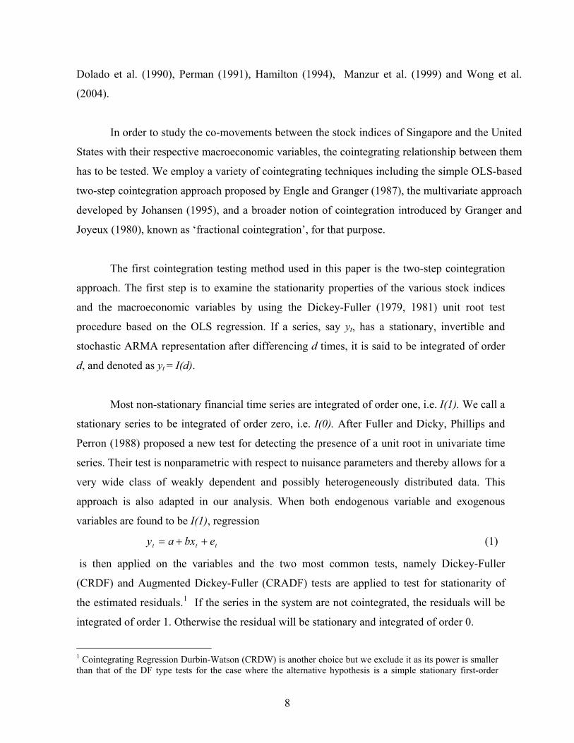
variables are found to be I(1), regression

ttt ebxay ++= (1)

is then applied on the variables and the two most common tests, namely Dickey-Fuller

(CRDF) and Augmented Dickey-Fuller (CRADF) tests are applied to test for stationarity of

the estimated residuals.1 If the series in the system are not cointegrated, the residuals will be

integrated of order 1. Otherwise the residual will be stationary and integrated of order 0.

1 Cointegrating Regression Durbin-Watson (CRDW) is another choice but we exclude it as its power is smaller than that of the DF type tests for the case where the alternative hypothesis is a simple stationary first-order

8

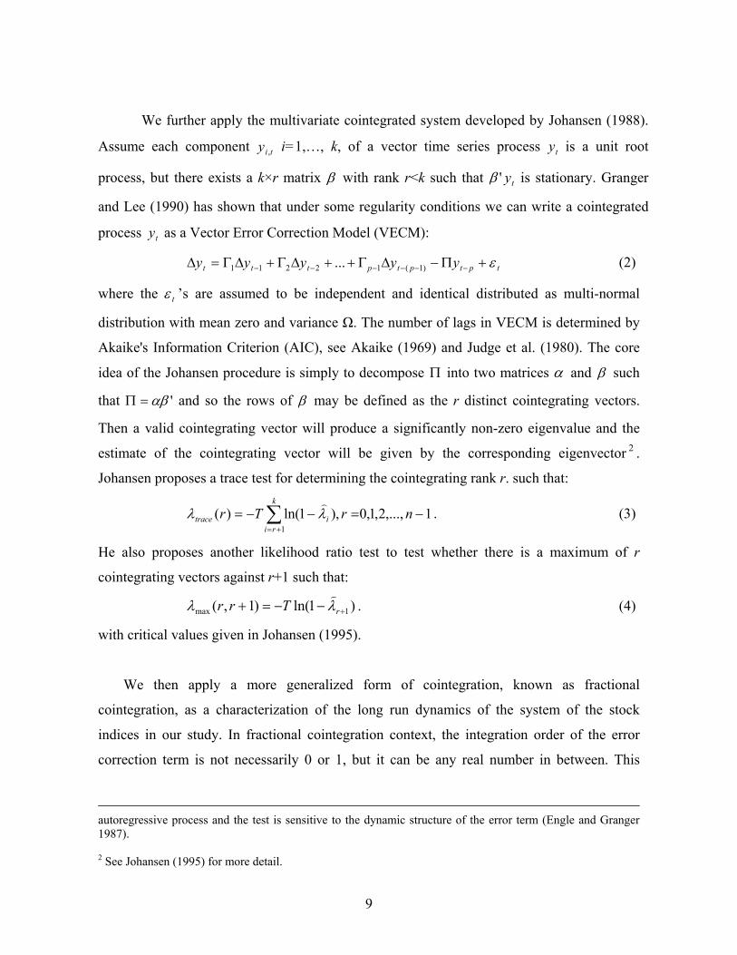
We further apply the multivariate cointegrated system developed by Johansen (1988).

Assume each component i=1,…, k, of a vector time series process is a unit root

process, but there exists a k×r matrix

tiy , ty

β with rank r<k such that ty'β is stationary. Granger

and Lee (1990) has shown that under some regularity conditions we can write a cointegrated

process as a Vector Error Correction Model (VECM): ty

tptptpttt yyyyy ε+Π−ΔΓ++ΔΓ+ΔΓ=Δ −−−−−− )1(12211 ... (2)

where the tε ’s are assumed to be independent and identical distributed as multi-normal

distribution with mean zero and variance Ω. The number of lags in VECM is determined by

Akaike's Information Criterion (AIC), see Akaike (1969) and Judge et al. (1980). The core

idea of the Johansen procedure is simply to decompose Π into two matrices α and β such

that 'αβ=Π and so the rows of β may be defined as the r distinct cointegrating vectors.

Then a valid cointegrating vector will produce a significantly non-zero eigenvalue and the

estimate of the cointegrating vector will be given by the corresponding eigenvector 2 .

Johansen proposes a trace test for determining the cointegrating rank r. such that:

1,...,2,1,0),1ln()(1

−=−−= ∑+=

nrTrk

riitrace λλ)

. (3)

He also proposes another likelihood ratio test to test whether there is a maximum of r

cointegrating vectors against r+1 such that:

)1ln()1,( 1max +−−=+ rTrr λλ)

. (4)

with critical values given in Johansen (1995).

We then apply a more generalized form of cointegration, known as fractional

cointegration, as a characterization of the long run dynamics of the system of the stock

indices in our study. In fractional cointegration context, the integration order of the error

correction term is not necessarily 0 or 1, but it can be any real number in between. This

autoregressive process and the test is sensitive to the dynamic structure of the error term (Engle and Granger 1987). 2 See Johansen (1995) for more detail.

9

allows obtaining more various mean reverting situations3. More specifically, a fractionally

integrated error correction term implies the existence of a long run equilibrium relationship,

as it can be shown to be mean reverting, though not exactly I(0). Despite its significant

persistence in the short run, the effect of a shock to the system eventually dissipates, so that

an equilibrium relationship among the system’s variables prevails in the long run.

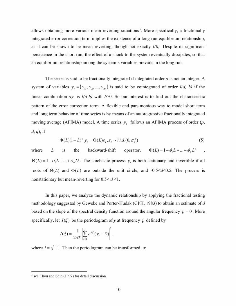
The series is said to be fractionally integrated if integrated order d is not an integer. A

system of variables is said to be cointegrated of order I(d, b) if the

linear combination

ntttt yyyy ,...,, 21=

tyα is I(d-b) with b>0. So our interest is to find out the characteristic

pattern of the error correction term. A flexible and parsimonious way to model short term

and long term behavior of time series is by means of an autoregressive fractionally integrated

moving average (AFIMA) model. A time series follows an AFIMA process of order (p,

d, q), if

ty

),0.(..~,)()1)(( 2εσεε diiLyLL ttt

d Θ=−Φ (5)

where L is the backward-shift operator, ,

. The stochastic process is both stationary and invertible if all

roots of and are outside the unit circle, and -0.5<d<0.5. The process is

nonstationary but mean-reverting for 0.5< d <1.

pp LLL φφ −−−=Φ ...1)( 1

qq LLL υυ +++=Θ ...1)( 1 ty

)(LΘ )(LΦ

In this paper, we analyze the dynamic relationship by applying the fractional testing

methodology suggested by Geweke and Porter-Hudak (GPH, 1983) to obtain an estimate of d

based on the slope of the spectral density function around the angular frequency 0=ξ . More

specifically, let )(ξI be the periodogram of y at frequency ξ defined by

2

1

)(2

1)( ∑=

−=T

tt

it yyeT

I ξ

πξ ,

where 1−=i . Then the periodogram can be transformed to:

3 see Chou and Shih (1997) for detail discussion.

10

⎪⎭

⎪⎬⎫

⎪⎩

⎪⎨⎧

⎥⎦

⎤⎢⎣

⎡−−+−= ∑ ∑ ∑

=

−

=

−

=+

T

t

T

k

kT

jkjjt kyyyy

Tyy

TI

1

1

1 1

2 )cos())((12)(121)( ξπ

ξ ,

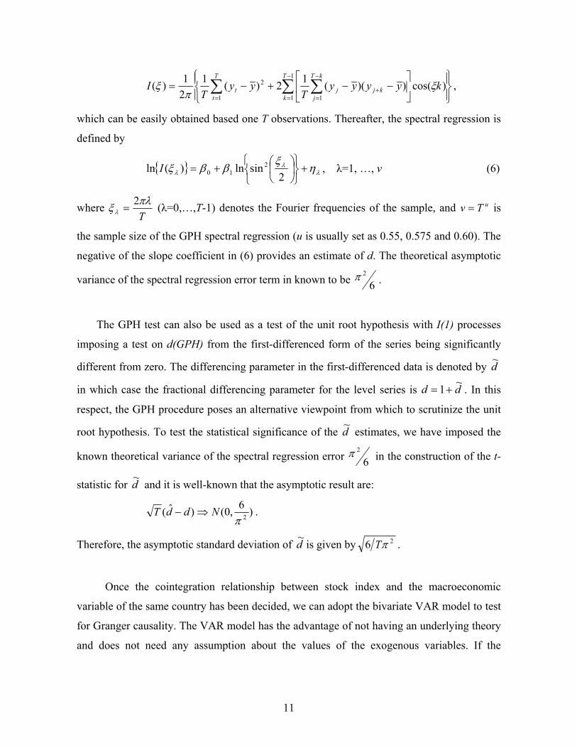
which can be easily obtained based one T observations. Thereafter, the spectral regression is

defined by

λλ

λ ηξ

ββξ +⎭⎬⎫

⎩⎨⎧

⎟⎠⎞

⎜⎝⎛+=

2sinln)(ln 2

10I , λ=1, …, v (6)

where Tπλξλ

2= (λ=0,…,T-1) denotes the Fourier frequencies of the sample, and is

the sample size of the GPH spectral regression (u is usually set as 0.55, 0.575 and 0.60). The

negative of the slope coefficient in (6) provides an estimate of d. The theoretical asymptotic

variance of the spectral regression error term in known to be

uTv =

62π .

The GPH test can also be used as a test of the unit root hypothesis with I(1) processes

imposing a test on d(GPH) from the first-differenced form of the series being significantly

different from zero. The differencing parameter in the first-differenced data is denoted by d~

in which case the fractional differencing parameter for the level series is dd ~1+= . In this

respect, the GPH procedure poses an alternative viewpoint from which to scrutinize the unit

root hypothesis. To test the statistical significance of the d~ estimates, we have imposed the

known theoretical variance of the spectral regression error 62π in the construction of the t-

statistic for d~ and it is well-known that the asymptotic result are:

)6,0()ˆ( 2πNddT ⇒− .

Therefore, the asymptotic standard deviation of d~ is given by 26 πT .

Once the cointegration relationship between stock index and the macroeconomic

variable of the same country has been decided, we can adopt the bivariate VAR model to test

for Granger causality. The VAR model has the advantage of not having an underlying theory

and does not need any assumption about the values of the exogenous variables. If the

11

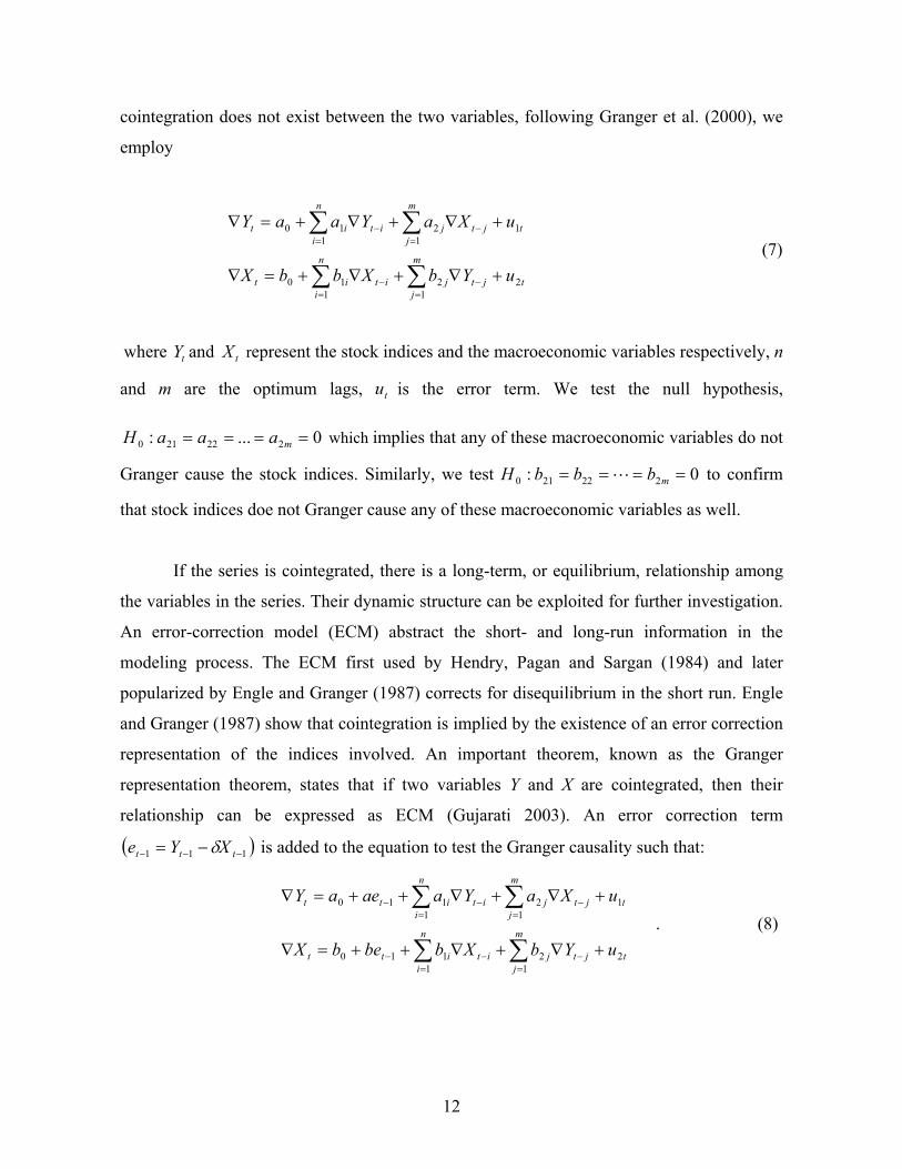
cointegration does not exist between the two variables, following Granger et al. (2000), we

employ

t

m

jjtj

n

iitit

t

m

jjtj

n

iitit

uYbXbbX

uXaYaaY

21

21

10

11

21

10

+∇+∇+=∇

+∇+∇+=∇

∑∑

∑∑

=−

=−

=−

=−

(7)

where and represent the stock indices and the macroeconomic variables respectively, n

and m are the optimum lags, is the error term. We test the null hypothesis,

which implies that any of these macroeconomic variables do not

Granger cause the stock indices. Similarly, we test

tY tX

tu

0...: 222210 ==== maaaH

0: 222210 ==== mbbbH L to confirm

that stock indices doe not Granger cause any of these macroeconomic variables as well.

If the series is cointegrated, there is a long-term, or equilibrium, relationship among

the variables in the series. Their dynamic structure can be exploited for further investigation.

An error-correction model (ECM) abstract the short- and long-run information in the

modeling process. The ECM first used by Hendry, Pagan and Sargan (1984) and later

popularized by Engle and Granger (1987) corrects for disequilibrium in the short run. Engle

and Granger (1987) show that cointegration is implied by the existence of an error correction

representation of the indices involved. An important theorem, known as the Granger

representation theorem, states that if two variables Y and X are cointegrated, then their

relationship can be expressed as ECM (Gujarati 2003). An error correction term

( 111 −−− −= ttt XYe )δ is added to the equation to test the Granger causality such that:

t

m

jjtj

n

iititt

t

m

jjtj

n

iititt

uYbXbbebX

uXaYaaeaY

21

21

110

11

21

110

+∇+∇++=∇

+∇+∇++=∇

∑∑

∑∑

=−

=−−

=−

=−−

. (8)

12

The existence of the cointegration implies causality among the set of variables as manifested

by 0>+ ba , and b denote speeds of adjustment (Engle and Granger 1987). If we do not

reject :

a

0H 022221 ==⋅⋅⋅== maaa and a = 0, it means that any of the macroeconomic

variables does not Granger cause the stock indices. Similarly, do not reject :

and b = 0 suggests that the stock indices does not Granger cause any

of the macroeconomic variables (Granger et al. 2000). The Akaike's Information (AIC) is

used to determine the optimum lag structures in the regressions (7) and (8), where n and m

are lags in the left hand and right hand side variables respectively; and and are

disturbance terms obeying the assumptions of the classical linear regression model.

0H

022221 ==== mbbb L

tu1 tu2

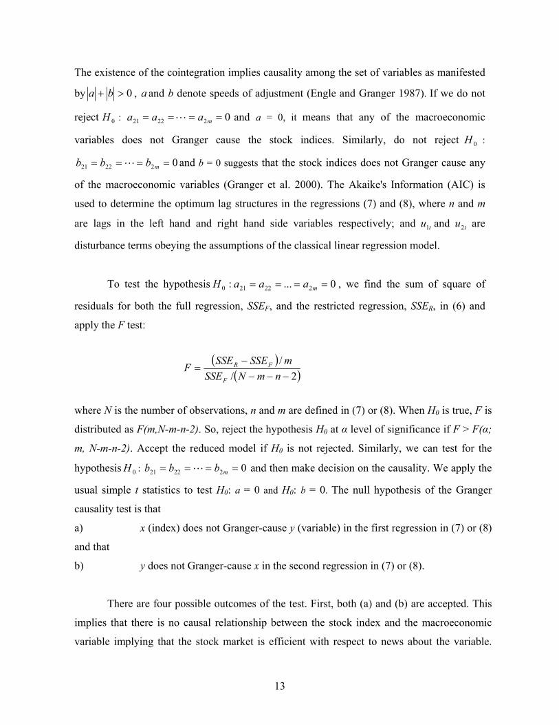
To test the hypothesis 0...: 222210 ==== maaaH , we find the sum of square of

residuals for both the full regression, SSEF, and the restricted regression, SSER, in (6) and

apply the F test:

( )( )2/

/−−−

−=

nmNSSEmSSESSEF

F

FR

where N is the number of observations, n and m are defined in (7) or (8). When H0 is true, F is

distributed as F(m,N-m-n-2). So, reject the hypothesis H0 at α level of significance if F > F(α;

m, N-m-n-2). Accept the reduced model if H0 is not rejected. Similarly, we can test for the

hypothesis : 0H 022221 ==== mbbb L and then make decision on the causality. We apply the

usual simple t statistics to test H0: a = 0 and H0: b = 0. The null hypothesis of the Granger

causality test is that

a) x (index) does not Granger-cause y (variable) in the first regression in (7) or (8)

and that

b) y does not Granger-cause x in the second regression in (7) or (8).

There are four possible outcomes of the test. First, both (a) and (b) are accepted. This

implies that there is no causal relationship between the stock index and the macroeconomic

variable implying that the stock market is efficient with respect to news about the variable.

13

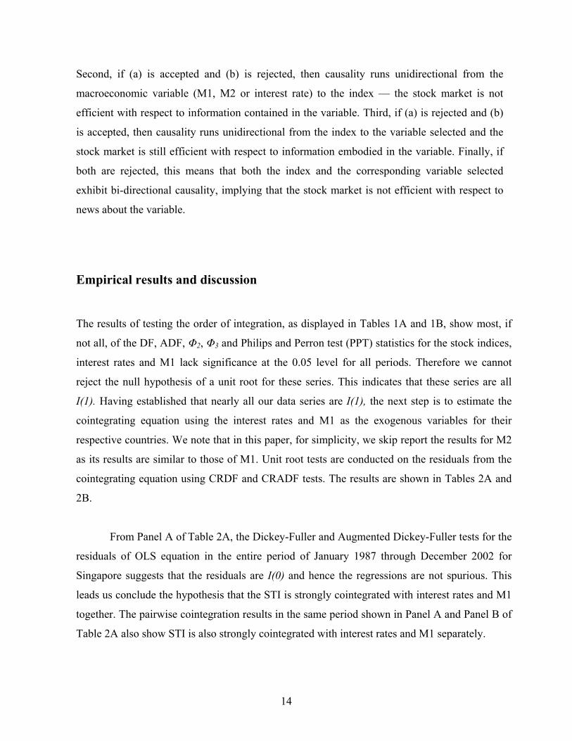
Second, if (a) is accepted and (b) is rejected, then causality runs unidirectional from the

macroeconomic variable (M1, M2 or interest rate) to the index — the stock market is not

efficient with respect to information contained in the variable. Third, if (a) is rejected and (b)

is accepted, then causality runs unidirectional from the index to the variable selected and the

stock market is still efficient with respect to information embodied in the variable. Finally, if

both are rejected, this means that both the index and the corresponding variable selected

exhibit bi-directional causality, implying that the stock market is not efficient with respect to

news about the variable.

Empirical results and discussion

The results of testing the order of integration, as displayed in Tables 1A and 1B, show most, if

not all, of the DF, ADF, Φ2, Φ3 and Philips and Perron test (PPT) statistics for the stock indices,

interest rates and M1 lack significance at the 0.05 level for all periods. Therefore we cannot

reject the null hypothesis of a unit root for these series. This indicates that these series are all

I(1). Having established that nearly all our data series are I(1), the next step is to estimate the

cointegrating equation using the interest rates and M1 as the exogenous variables for their

respective countries. We note that in this paper, for simplicity, we skip report the results for M2

as its results are similar to those of M1. Unit root tests are conducted on the residuals from the

cointegrating equation using CRDF and CRADF tests. The results are shown in Tables 2A and

2B.

From Panel A of Table 2A, the Dickey-Fuller and Augmented Dickey-Fuller tests for the

residuals of OLS equation in the entire period of January 1987 through December 2002 for

Singapore suggests that the residuals are I(0) and hence the regressions are not spurious. This

leads us conclude the hypothesis that the STI is strongly cointegrated with interest rates and M1

together. The pairwise cointegration results in the same period shown in Panel A and Panel B of

Table 2A also show STI is also strongly cointegrated with interest rates and M1 separately.

14

We further investigate the cointegration relationship of the variables in the sub-periods to

capture the evolving relations across the asset price turbulence in the past two decades. The

results in Panel A of Table 2A lead us formulate the hypothesis that the STI is strongly

cointegrated with interest rates and M1 together strongly in the sub-period 1987-1996 and

marginally in the sub-period 1997-2002. We turn to investigate the pairwise cointegration

relationship of the STI with each individual macroeconomic variable used in our study. The

results in Panel B of Table 2A show that the STI is marginally cointegrated with interest rate for

both sub-periods 1987-1996 and 1997-2002; while strongly cointegrated with M1 in the sub-

period 1987-1996 but not cointegrated with it in the sub-period 1997-2002. Thus the Singapore

stock market maintains a stable equilibrium with interest rate and M1 in the long run for the

entire period as well as both sub-periods from 1987-1996 and 1997-2002. However, the

cointegration relationship is weakened after 1997 Asian crisis, with only marginal cointegration

between STI and interest rate.

From Panels A and B of Table 3A, our Johansen multivariate cointegration test results

for the case of Singapore lead us draw a conclusion similar to that from the two-step

cointegration test: the Singapore stock market maintains a stable equilibrium with interest rate

and M1 in the long run for the entire period as well as for the 1987-1996 sub-period. However,

the results in Panel C of the Table 3A cannot reject null that there is no cointegration

relationship among STI, the interest rate and M1 for the 1997-2002 sub-period; this is different

from the two-step test results. But a weakening trend of the cointegration relationship can be

observed in both analyses.

For comparison, we now turn to study the cointegration relationship of the stock index

with the macroeconomic variables of the interest rate and money supply (M1) in the United

States. Table 2B shows that the results are significantly different for the United States. There is

no cointegration for the set of variables jointly with the S&P 500 composite nor is there pairwise

cointegration of the S&P 500 with each of the variables for the entire period from January 1982

to December 2002 and for the sub-period from January 1987 to December 1996. However it is

interesting to note that the cointegration relationship of the S&P 500 with both variables, M1

and interest rate jointly are significant strongly for the sub-period from January 1982 to

15

December 1986 series and marginally for the last sub-period from January 1997 to December

2002. In terms of the cointegration relationship between index and each of the variables, it is

found that that there is cointegration of the S&P500 with interest rates for the sub-periods 1982-

1986 and 1997-2002 and cointegration of S&P500 with M1 for the sub-period 1982 – 1986.

For the US data, the Johansen multivariate analysis in Table 3B reveals almost same

evidence as those from the two–step test for the overall period but some differences in the sub-

periods as follows. The information in Panel A of Table 3B suggests that S&P 500 composite

index, U.S. interest rate and money supply M1 cannot form a stationary system of linear

equilibrium in the entire period but Panel B of Table 3B shows strong evidence of cointegration

in the 1982-1986 sub-period; implying that at least three unique cointegrating vectors are

available for the multivariate system. Panel C of Table 3B shows that after the 1987 stock

market turbulence, there is only one cointegrating vector available for the system, a much

weaker evidence as compared with the 1982-1986 sub-period. The results for this last sub-period

covering the 1997 Asian financial crisis and 2000 internet bubble burst are shown in Panel D. In

this period, the Johansen analysis cannot reveal any evidence of cointegration. Thus we

conclude from Johansen test that the cointegration relationship between S&P 500 and

macroeconomic variables of interest rate and M1 does exist at beginning but becomes weaker

and weaker across the three sub-periods respectively marked by its own characteristic financial

events.

To extend our research to a broader of horizon, we appoint the fractional integration test,

a more generalized form of integration concept, in our cointegration analysis to first test the unit

root characteristic of each variable we are interested in, and then test the stationarity property for

the system residual. Basically, this is a similar procedure to the two-step cointegration test, but it

extends our scrutiny beyond a world of integer and allows us to examine the fractional

integration order for each variable and the residuals of the cointegration regression. Table 4

reveals the fractional integration order for every variable in each period for Singapore and for

USA. The results show that the integration order for all the variables, though not exactly

integrated at order 1, are roughly near 1. This implies that all variables still contain a unit root.

Table 5 shows the fractional cointegration test on the residuals obtained from the various

16

Johansen multivariate systems established. We prefer Johansen residual to OLS residual because

the OLS regression coefficients are likely to be inconsistent when the explanatory variables are

contemporaneously correlated with the disturbance term. On the other hand, Johansen

multivariate system is based on the maximum likelihood estimation and thus avoids the danger

of inconsistence as in OLS estimation. Panel A of Table 5 shows that in the entire period the

three estimates of integration order, d(0.55), d(0.575) and d(0.6), though not less 0.5 as we

expect to see, but are much less than 1; this implies that the residuals are strongly mean-

reverting. In the sub-period before 1997 financial crisis, all the integration order estimates are

less than 0.5, implying that the residual for the system before 1997 is stationary and thus there is

cointegration relationship in the system. In the second sub-period of the Singapore case, the

estimates are close to 1, implying that the Johansen system is non-stationary and there is no

cointegration relationship in the system. This confirms the results obtained from the Johansen

test. On the other hand, Panel B of Table 5 shows for the results of U.S. case that the system of

the entire period is slightly mean-reverting. But, the results for the first two sub-periods show

evidence of stationarity to different levels: (1) three estimates in the period 1982-1986 are less

than 0.5 and thus the system is in equilibrium; (2) only the d(0.575) estimate for the period after

the 1987 stock turbulence and before 1997 financial crisis is less than 0.5; and (3) in the last

sub-period, all three estimates are larger than 1, which means strong non-stationarity.

From the above results, it is clear that both Singapore and US stock markets did possess

equilibrium relationship with M1 and interest rate at the early days. However these stable

systems were impaired by a series of famous financial turbulence during the past two decades

and eventually disappeared for the U.S. This may suggest that monetary authority may take

action to respond to the asset price turbulence in order to maintain the stability of monetary

economy and thus break the existing equilibrium between stock markets and macroeconomic

variables like interest rate and M1.

We now turn to study the Granger causality relationship between the stock index and

each of the macroeconomic variables and depict the results in Tables 6A and 6B. ECM is

employed to test for the Granger Causality, if cointegration is found between the stock markets

with the macroeconomic variables, while VAR model is employed, if otherwise. In the entire

17

period, STI index is found to lead Singapore interest rate in the long run while money supply

M1 can stir movements in STI index. However, in the 1987-1996 period, the causality runs bi-

directionally between both pairs of variables, indicating a sensitive and hectic time of the both

stock market and monetary authority, while in the post-crisis sub-period (1997-2002), there is

only granger causality running from STI to interest rate. Overall, we observe a consistent

influence from the stock market to interest rate of Singapore.

On the other hand, Table 6B shows no causal nexus between any pair of variables in the

full sample for the United States. However, before the 1987 stock crisis, there is evidence that

money supply M1 drives S&P 500 index in the long run but there is no causal relation between

stock market and macroeconomic variables in the sub-period of 1987-1996. However, the causal

relationship comes back in the last sub-period covering the Asian Financial Crisis and the

Internet Stock Bubble. It can be observed that short-run causality runs uni-directionally from

stock market to interest rate of the United States and there exists bi-directionality between stock

market and money supply M1.

Conclusion

This study investigates the long run and short run relationships between the major stock indices

of Singapore and the United States and some macroeconomic variables, like the measure of

money supply, M1 and interest rates by means of time series analysis for the period covering

January 1982 to December 2002. Our cointegration analysis suggest that changes in Singapore’s

stock prices in general do form a long run equilibrium relationship with interest rate and M1 but

the same does not apply to the case of the United States. We further divide the overall study

period into three sub-periods for Singapore and United States data in order to focus on evolving

relation between stock price indices and macroeconomic variables on different market

conditions. It is found that before 1997 Asian financial crisis, stock markets in Singapore were

cointegrated with interest rate and money supply. However this equilibrium relationship has

rather weakened after the crisis. In the U.S. markets, stock prices were strongly cointegrated

18

with macro-economic variables before 1987 equity crisis and the equilibrium was impaired after

1987 crisis and ultimately disappeared after 1997 Asian Crisis.

Our fractional cointegration results show that in the entire period the residuals of the

Johansen multivariate system are non-stationary but strongly mean-reverting in the entire period

for both Singapore and USA. The Johansen multivariate system for both countries experience

cointegration in the earlier sub-period but become but non-stationary and not mean-reverting in

the sub-period after 1997 financial crisis. This finding is basically consistent with the

cointegration findings in both countries such that both Singapore and US stock markets did

possess equilibrium relationship with M1 and interest rate at the early days. However these

stable systems were impaired by a series of famous financial turbulence during the past two

decades and eventually weakened for Singapore and disappeared for the U.S. This may suggest

that monetary authority may take action to respond to the asset price turbulence in order to

maintain the stability of monetary economy and thus break the existing equilibrium between

stock markets and macroeconomic variables like interest rate and M1. Another explanation is

the market becomes more efficient in both markets after 1997 financial crisis. Finally, the results

from the Granger Causality tests seem to support the view that the level of the stock markets

might be used by central bank as an indicator to adjust monetary policy.

The cointegration and causality findings in our paper might lend additional support to

the investors in their investment decisions in the US and Singapore stock markets. Investors

could perhaps get new insights by incorporating these results with our previous findings of

technical analysis (Wong et al. 2001, 2003). Since stock investment is always a risky

proposition, the decision- making process should be built upon the inferences drawn from

various alternative approaches such fundamental analysis (Thompson and Wong 1991, Wong

and Chan 2004), the stochastic dominance approach (Wong and Li 1999, and Wong et al.

2005), and/or a study on the economic situation or financial anomalies (Manzur, et al. 1999,

Wan and Wong 2001, and Fong et al. 2005). Perhaps one could also apply advanced time

series analysis (Wong and Miller 1990, Tiku et al. 2000 and Wong and Bian 2005) and/or

Bayesian estimation (Matsumura et al. 1990 and Wong and Bian 2000) to improve the

chances of success in stock investments.

19

References: Akaike, H. (1969), “Fitting Autoregressive Models for Prediction”, Annals of The Institute of Statistical Mathematics, 21, 243-347. Bernanke, B.S. and Gertler, M. (1999), “Monetary Policy and Asset Price Volatility”, Federal Reserve Bank of Kansas City, Economic Review, 84, 17-51. Bernanke, B.S. and Gertler, M. (2001), “Should Central Bank Respond to Movement in Asset Prices”, American Economic Review, 91, 2, 253. Chou, W. and Shih, Y. (1997), “Long-run purchasing power parity and long-term memory: evidence from Asian newly industrialized countries”, Applied Economics Letters, 4, 575-578. Dickey, D.A. and Fuller, W.A. (1979), “Distribution of the estimators for autoregressive time series with a unit root”, Journal of the American Statistical Association, 74, 427-431. Dickey, D.A. and Fuller, W.A. (1981), “Likelihood ratio statistics for autoregressive time series with unit roots”, Econometrica, 49(4), 1057-72. Dolado, J., Jenkinson, T. and Sosvilla-Rivero, S. (1990), “Cointegration and unit roots”, Journal of Economic Surveys, 3, 251-76. Engle, R.F. and Granger, C.W.J. (1987), “Cointegration and error correction: representation, estimation and testing”, Econometrica, 55, 251-76. Fong, W.M., Lean, H.H. and Wong, W.K. (2005), Stochastic Dominance and the Rationality of the Momentum Effect across Markets, Journal of Financial Markets, 8, 89-109. Geweke, J. and Porter-Hudak, S. (1983), “The estimation and application of long memory time series models”, Journal of Time Series Analysis, 4, 221-238. Goodhart, C. A. and Hofmann, B. (2000), “Financial Variables and the Conduct of Monetary Policy”, Sveriges Riksbank (Central Bank of Sweden) working paper Series, 2000, No. 112. Goodhart, C. A. and Hofmann, B. (2001), “Asset Prices, Financial Conditions, and the Transmission of Monetary Policy”, Federal Reserve Bank of San Francisco working paper, 2001, Issue March. Granger, C.W.J. and Joyeux, R. (1980), “An Introduction to Long-memory Models and Fractional Differencing”, Journal of Time Series Analysis, 1, 15-39. Granger, C.W.J. (1981). “Some Properties of Time Series Data and their Use in Econometric Model Specification”, Journal of Econometrics, 16,121-130. Granger, C.W.J. (1987), ‘Developments in the study of cointegrated economic variables”, Bulletin of Economics and Statistics, 48, 213-28.

20

Granger, C.W.J. and Lee, T. (1990), “Multicointegration”, in Rhodes, G. F. and Fomby, T. B., Advances in Econometrics,.8, Greenwich CT JAI Press, 71-84. Granger, Clive W. J., Huang, B. and Yang, Chin-Wei (2000), “A bivariate causality between stock prices and exchange rates: evidence from recent Asian flu” The Quarterly Review of Economics and Finance 40, 337-354. Hamilton, J. (1994), Time Series Analysis, 1st Edition, Princeton University Press. Hendry, D.F., Pagan, A.R. and Sargan, J.D. (1984), “Dynamic Specifications”, Chapter 8 in Z. Griliches and M.D. Intrilligator (eds.), The Handbook of Econometrics, North Holland, Amsterdam. Ho, Y. (1983), “Money Supply and Equity Prices: An Empirical Note on Far Eastern Countries”, Economic Letters, 11, 161 – 165. Johansen, S. (1988a), “The Mathematical Structure of Error Correction Models”, Contemporary Mathematics, 8, 359-86. Johansen, S. (1988b), “Statistical Analysis of Cointegration Vector”, Journal of Economic Dynamics and Control, 12, 231-254. Johansen, S. (1995), “Likelihood-inference in Cointegrated Vector Auto-regressive Models”, Oxford: OUP. Judge, G.G., Griffiths, W.E., Hill, R.C. and Lee, T.C., The Theory and Practice of Econometrics, John Wiley, New York, 1980. Kwon, C.S and Shin, T. S. (1999), “Cointegration and Causality between Macroeconomic Variables and Stock Market Returns”, Global Finance Journal, 10(1), 71 – 81. Manzur, M., Wong, W.K. and Chau, I.C. (1999), “Measuring international competitiveness: experience from East Asia”, Applied Economics, 31, 1383-1391. Matsumura, E. M., Tsui, K. W. and Wong, W. K. (1990) An Extended Multinomial-Dirichlet Model for Error Bounds for Dollar-Unit Sampling, Contemporary Accounting Research, 6(2-I), 485-500. Mayasami, R. C. and Koh, T. S. (2000), “A Vector Error Correction Model of the Singapore Stock Market”, International Review of Economics and Finance, 9, 79 – 96. Mukherjee, T. K. and Naka, A. (1995), “Dynamic relations between macroeconomic variables and the Japanese stock market: an application of a vector error-correction model”, Journal of Financial Research, 18(2), 223 – 237. Peevey, R.M., Uselton, G.C. and Moroney, J. R. (1993), “The Individual Investor in the Market: Forming a Belief Regarding Market Efficiency”, Financial Services Review, 2(2), 87 – 96. Perman, R. (1991), “Cointegration: An Introduction to the literature”, Journal of Economic Studies, 18, 3-30. Phillips, P.C.B. and Perron, P. (1988), “Testing for a Unit Rppt in Time Series Regression”, Biometrica, 75, 335-346.

21

Smets, F. (1997), “Financial Asset Prices and Monetary Policy: Theory and Evidence”, in P. Lowe (ed.), Monetary Policy and Inflation Targeting, Proceedings of a Conference, Reserve Bank of Australia, Sydney, 212–237. Stock, J. (1987), “Asymptotic Properties of Least Squares Estimators of Cointegrating Vectors”, Econometrica, 55, 381 – 386. Thompson, H. E. and Wong, W. K. (1991), “On the Unavoidability of `Unscientific' Judgment in Estimating the Cost of Capital”, Managerial and Decision Economics, 12, 27-42. Tiku, M. L., Wong, W. K., Vaughan, D. C. and Bian G. (2000), “Time Series Models with Nonnormal Innovations: Symmetric Location-scale Distributions,” Journal of Time Series Analysis, 21(5), 571-596. Wan, Henry Jr. and Wong, W.K. (2001), “Contagion or Inductance: Crisis 1997 Reconsidered,” Japanese Economic Review, 52(4), 372-380. Wong, W. K. and Bian, G. (2000), Robust Bayesian Inference in Asset Pricing Estimation, Journal of Applied Mathematics & Decision Sciences, 4(1), 65-82. Wong, W.K. and Bian, G. (2005), “Estimating Parameters in Autoregressive Models with asymmetric innovations”, Statistics and Probability Letters, 71, 61-70. Wong, W K and Chan, R. (2004), “The Estimation of the Cost of Capital and its Reliability”, Quantitative Finance, 4(3), 365 – 372. Wong W. K., Chew, B. K. and Sikorski, D. (2001), “Can P/E Ratio and Bond Yield be used to beat Stock Markets?”, Multinational Finance Journal, 5(1), 59-86. Wong, W. K. and Li, C. K. (1999), “A Note on Convex Stochastic Dominance Theory”, Economics Letters, 62, 293-300. Wong, W. K., Manzur, M. and Chew, B. K. (2003), “How Rewarding is Technical Analysis? Evidence from Singapore Stock Market”, Applied Financial Economics, 13(7), 543-551. Wong, W. K. and Miller, R. B. (1990), “Analysis of ARIMA-Noise Models with Repeated Time Series”, Journal of Business and Economic Statistics, 8(2), 243-250. Wong, W. K., Thompson, H.E., Wei, S. and Chow, Y.F. (2005), “Do Winners perform better than Losers? A Stochastic Dominance Approach”, Advances in Quantitative Analysis of Finance and Accounting, (forthcoming). Wu, Y. (2001), “Exchange Rates, Stock Prices, and Money Markets: Evidence from Singapore”, Journal of Asian Economics, 12, 445 – 458.

22

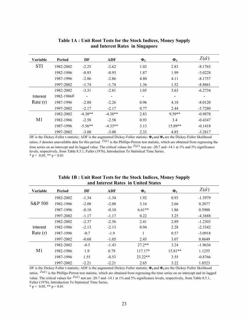
Table 1A : Unit Root Tests for the Stock Indices, Money Supply and Interest Rates in Singapore

Variable Period DF ADF Φ2 Φ3

)ˆ(αZ

STI 1982-2002 -2.25 -2.62 1.02 2.83 -8.1765 1982-1986 -0.93 -0.93 1.87 1.99 -3.0228 1987-1996 -2.86 -2.86 4.80 4.11 -8.1757 1997-2002 -1.74 -1.74 1.36 1.52 -8.8861 1982-2002 -3.31 -2.81 1.05 5.63 -6.2734

Interest 1982-1986# - - - - - Rate (r) 1987-1996 -2.88 -2.26 0.96 4.18 -8.0120

1997-2002 -2.17 -2.17 0.77 2.44 -3.7280 1982-2002 -4.38** -4.38** 2.83 9.59** -0.9878

M1 1982-1986 -2.58 -2.58 0.93 3.4 -0.4347 1987-1996 -5.56** -4.33** 3.13 15.89** -0.1418 1997-2002 -3.08 -3.08 2.32 4.85 -3.2817

DF is the Dickey-Fuller t-statistic; ADF is the augmented Dickey-Fuller statistic; Φ2 and Φ3 are the Dickey-Fuller likelihood ratios, # denotes unavailable data for this period. )(α)Z is the Phillips-Perron test statistic, which are obtained from regressing the time series on an intercept and its lagged value. The critical values for )(α)Z test are -20.7 and -14.1 at 1% and 5% significance levels, respectively, from Table 8.5.1, Fuller (1976), Introduction To Statistical Time Series. * p < 0.05, ** p < 0.01

Table 1B : Unit Root Tests for the Stock Indices, Money Supply and Interest Rates in United States

Variable Period DF ADF Φ2 Φ3)ˆ(αZ

1982-2002 -1.34 -1.34 1.92 0.93 -1.3979 S&P 500 1982-1986 -2.08 -2.08 3.16 2.66 0.2077

1987-1996 -0.10 -0.10 6.61** 1.86 0.5900 1997-2002 -1.17 -1.17 0.22 3.25 -4.3688 1982-2002 -2.37 -2.56 2.41 2.89 -1.2303

Interest 1982-1986 -2.13 -2.13 0.94 2.28 -2.3342 Rate (r) 1987-1996 -0.7 -1.9 1 0.57 -3.0918

1997-2002 -0.68 -1.05 2.45 3.07 0.8649 1982-2002 -0.5 -1.43 27.2** 3.24 -1.9636

M1 1982-1986 1.9 0.79 117.17* 15.81** 1.1255 1987-1996 1.55 -0.53 23.22** 3.55 -0.8766 1997-2002 -2.21 -2.21 2.65 3.22 1.8523

DF is the Dickey-Fuller t-statistic; ADF is the augmented Dickey-Fuller statistic; Φ2 and Φ3 are the Dickey-Fuller likelihood ratios. )(α)Z is the Phillips-Perron test statistic, which are obtained from regressing the time series on an intercept and its lagged value. The critical values for )(α)Z test are -20.7 and -14.1 at 1% and 5% significance levels, respectively, from Table 8.5.1, Fuller (1976), Introduction To Statistical Time Series. * p < 0.05, ** p < 0.01

23

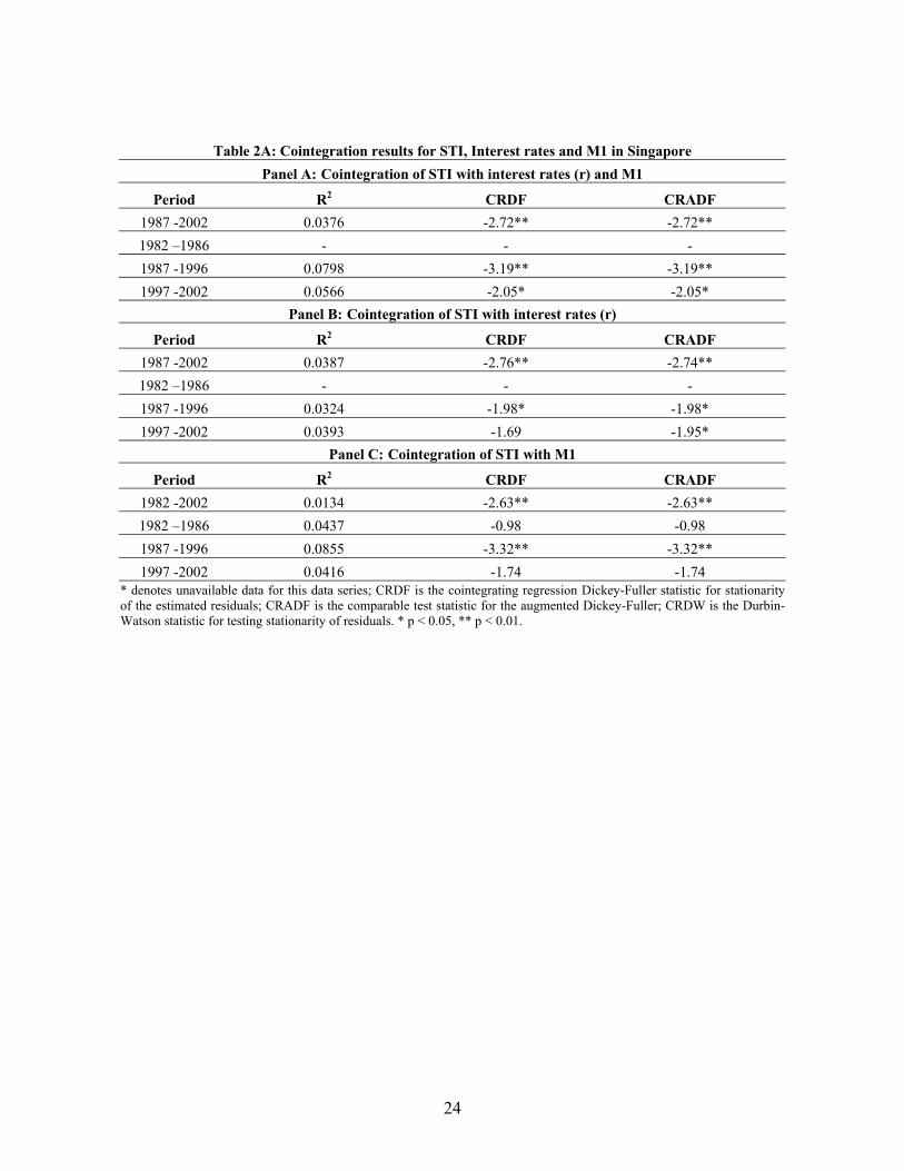
Table 2A: Cointegration results for STI, Interest rates and M1 in Singapore Panel A: Cointegration of STI with interest rates (r) and M1

Period R2 CRDF CRADF 1987 -2002 0.0376 -2.72** -2.72** 1982 –1986 - - - 1987 -1996 0.0798 -3.19** -3.19** 1997 -2002 0.0566 -2.05* -2.05*

Panel B: Cointegration of STI with interest rates (r)

Period R2 CRDF CRADF 1987 -2002 0.0387 -2.76** -2.74** 1982 –1986 - - - 1987 -1996 0.0324 -1.98* -1.98* 1997 -2002 0.0393 -1.69 -1.95*

Panel C: Cointegration of STI with M1

Period R2 CRDF CRADF 1982 -2002 0.0134 -2.63** -2.63** 1982 –1986 0.0437 -0.98 -0.98 1987 -1996 0.0855 -3.32** -3.32** 1997 -2002 0.0416 -1.74 -1.74

* denotes unavailable data for this data series; CRDF is the cointegrating regression Dickey-Fuller statistic for stationarity of the estimated residuals; CRADF is the comparable test statistic for the augmented Dickey-Fuller; CRDW is the Durbin-Watson statistic for testing stationarity of residuals. * p < 0.05, ** p < 0.01.

24

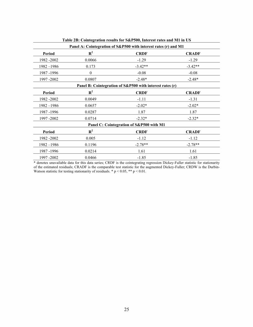
Table 2B: Cointegration results for S&P500, Interest rates and M1 in US Panel A: Cointegration of S&P500 with interest rates (r) and M1

Period R2 CRDF CRADF 1982 -2002 0.0066 -1.29 -1.29 1982 –1986 0.173 -3.42** -3.42** 1987 -1996 0 -0.08 -0.08 1997 -2002 0.0807 -2.48* -2.48*

Panel B: Cointegration of S&P500 with interest rates (r)

Period R2 CRDF CRADF 1982 -2002 0.0049 -1.11 -1.31 1982 –1986 0.0657 -2.02* -2.02* 1987 -1996 0.0287 1.87 1.87 1997 -2002 0.0714 -2.32* -2.32*

Panel C: Cointegration of S&P500 with M1

Period R2 CRDF CRADF 1982 -2002 0.005 -1.12 -1.12 1982 –1986 0.1196 -2.78** -2.78** 1987 -1996 0.0214 1.61 1.61 1997 -2002 0.0466 -1.85 -1.85

* denotes unavailable data for this data series; CRDF is the cointegrating regression Dickey-Fuller statistic for stationarity of the estimated residuals; CRADF is the comparable test statistic for the augmented Dickey-Fuller; CRDW is the Durbin-Watson statistic for testing stationarity of residuals. * p < 0.05, ** p < 0.01.

25

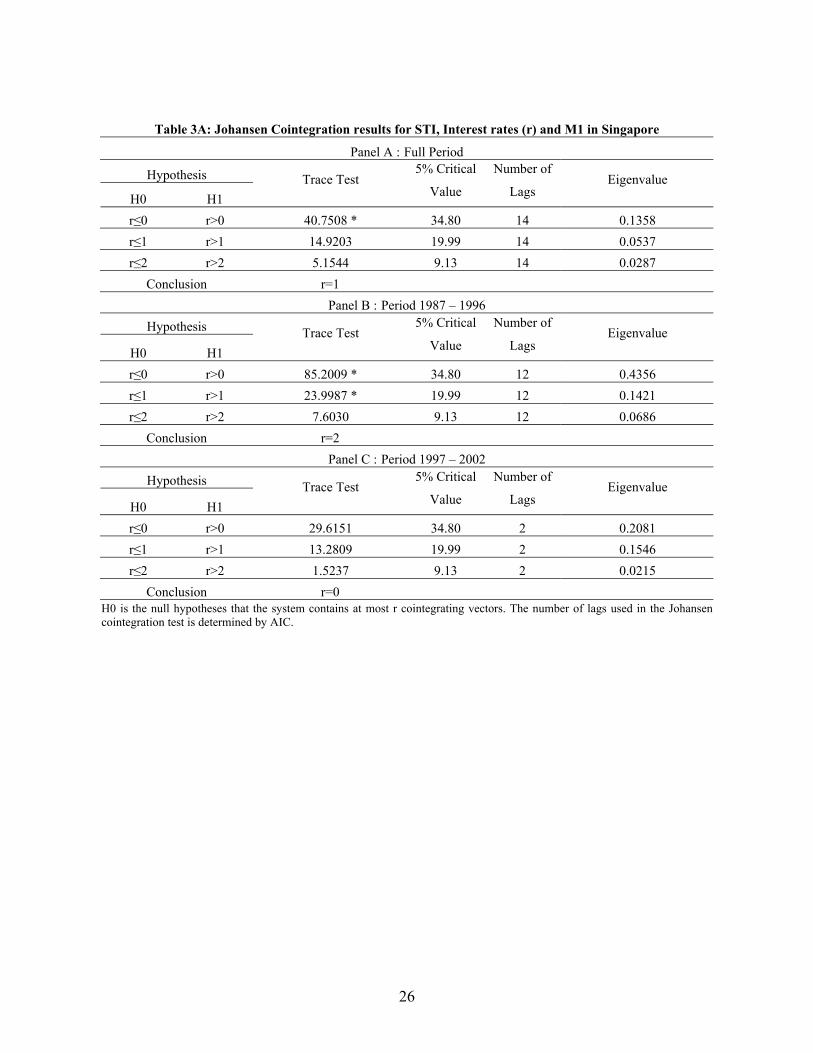
Table 3A: Johansen Cointegration results for STI, Interest rates (r) and M1 in Singapore

Panel A : Full Period

Hypothesis

H0 H1 Trace Test

5% Critical

Value

Number of

Lags Eigenvalue

r≤0 r>0 40.7508 * 34.80 14 0.1358 r≤1 r>1 14.9203 19.99 14 0.0537 r≤2 r>2 5.1544 9.13 14 0.0287

Conclusion r=1 Panel B : Period 1987 – 1996

Hypothesis

H0 H1 Trace Test

5% Critical

Value

Number of

Lags Eigenvalue

r≤0 r>0 85.2009 * 34.80 12 0.4356 r≤1 r>1 23.9987 * 19.99 12 0.1421 r≤2 r>2 7.6030 9.13 12 0.0686

Conclusion r=2 Panel C : Period 1997 – 2002

Hypothesis

H0 H1 Trace Test

5% Critical

Value

Number of

Lags Eigenvalue

r≤0 r>0 29.6151 34.80 2 0.2081 r≤1 r>1 13.2809 19.99 2 0.1546 r≤2 r>2 1.5237 9.13 2 0.0215

Conclusion r=0 H0 is the null hypotheses that the system contains at most r cointegrating vectors. The number of lags used in the Johansen cointegration test is determined by AIC.

26

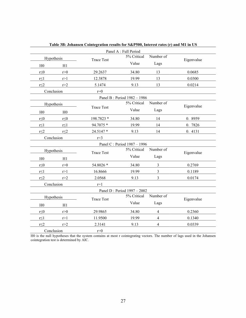
Table 3B: Johansen Cointegration results for S&P500, Interest rates (r) and M1 in US

Panel A : Full Period

Hypothesis

H0 H1 Trace Test

5% Critical

Value

Number of

Lags Eigenvalue

r≤0 r>0 29.2637 34.80 13 0.0685 r≤1 r>1 12.3878 19.99 13 0.0300 r≤2 r>2 5.1474 9.13 13 0.0214

Conclusion r=0 Panel B : Period 1982 – 1986

Hypothesis

H0 H0 Trace Test

5% Critical

Value

Number of

Lags Eigenvalue

r≤0 r≤0 198.7823 * 34.80 14 0．8959 r≤1 r≤1 94.7075 * 19.99 14 0．7826 r≤2 r≤2 24.5147 * 9.13 14 0．4131

Conclusion r=3 Panel C : Period 1987 – 1996

Hypothesis

H0 H1 Trace Test

5% Critical

Value

Number of

Lags Eigenvalue

r≤0 r>0 54.8026 * 34.80 3 0.2769 r≤1 r>1 16.8666 19.99 3 0.1189 r≤2 r>2 2.0568 9.13 3 0.0174

Conclusion r=1 Panel D : Period 1997 – 2002

Hypothesis

H0 H1 Trace Test

5% Critical

Value

Number of

Lags Eigenvalue

r≤0 r>0 29.9865 34.80 4 0.2360 r≤1 r>1 11.9500 19.99 4 0.1340 r≤2 r>2 2.3141 9.13 4 0.0339

Conclusion r=0 H0 is the null hypotheses that the system contains at most r cointegrating vectors. The number of lags used in the Johansen cointegration test is determined by AIC.

27

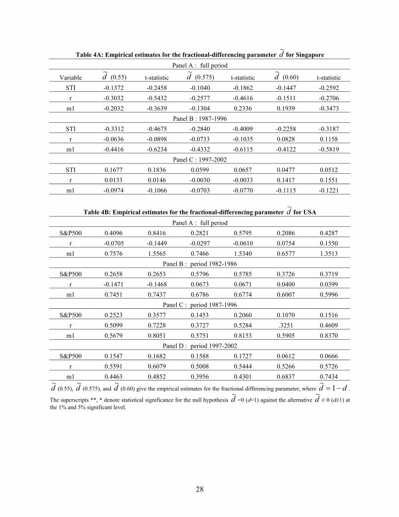
Table 4A: Empirical estimates for the fractional-differencing parameter d~ for Singapore Panel A : full period

Variable d~ (0.55) t-statistic d~ (0.575) t-statistic d~ (0.60) t-statistic STI -0.1372 -0.2458 -0.1040 -0.1862 -0.1447 -0.2592

r -0.3032 -0.5432 -0.2577 -0.4616 -0.1511 -0.2706 m1 -0.2032 -0.3639 -0.1304 0.2336 0.1939 -0.3473

Panel B : 1987-1996 STI -0.3312 -0.4675 -0.2840 -0.4009 -0.2258 -0.3187

r -0.0636 -0.0898 -0.0733 -0.1035 0.0828 0.1158 m1 -0.4416 -0.6234 -0.4332 -0.6115 -0.4122 -0.5819

Panel C : 1997-2002 STI 0.1677 0.1836 0.0599 0.0657 0.0477 0.0512

r 0.0133 0.0146 -0.0030 -0.0033 0.1417 0.1551 m1 -0.0974 -0.1066 -0.0703 -0.0770 -0.1115 -0.1221

Table 4B: Empirical estimates for the fractional-differencing parameter d~ for USA Panel A : full period

S&P500 0.4096 0.8416 0.2821 0.5795 0.2086 0.4287 r -0.0705 -0.1449 -0.0297 -0.0610 0.0754 0.1550

m1 0.7576 1.5565 0.7466 1.5340 0.6577 1.3513 Panel B : period 1982-1986

S&P500 0.2658 0.2653 0.5796 0.5785 0.3726 0.3719 r -0.1471 -0.1468 0.0673 0.0671 0.0400 0.0399

m1 0.7451 0.7437 0.6786 0.6774 0.6007 0.5996 Panel C : period 1987-1996

S&P500 0.2523 0.3577 0.1453 0.2060 0.1070 0.1516 r 0.5099 0.7228 0.3727 0.5284 .3251 0.4609

m1 0.5679 0.8051 0.5751 0.8153 0.5905 0.8370 Panel D : period 1997-2002

S&P500 0.1547 0.1682 0.1588 0.1727 0.0612 0.0666 r 0.5591 0.6079 0.5008 0.5444 0.5266 0.5726

m1 0.4463 0.4852 0.3956 0.4301 0.6837 0.7434

d~ (0.55), d~ (0.575), and d~ (0.60) give the empirical estimates for the fractional differencing parameter, where dd −=1~.

The superscripts **, * denote statistical significance for the null hypothesis d~ =0 (d=1) against the alternative d~ ≠ 0 (d≠1) at the 1% and 5% significant level.

28

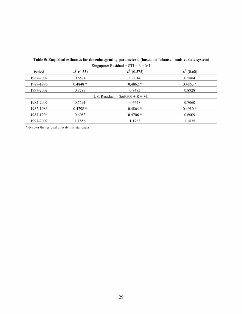
Table 5: Empirical estimates for the cointegrating parameter d (based on Johansen multivariate system)

Singapore: Residual = STI + R + M1 Period d (0.55) d (0.575) d (0.60)

1987-2002 0.6574 0.6014 0.5884 1987-1996 0.4848 * 0.4862 * 0.4863 * 1997-2002 0.8798 0.9493 0.8928

US: Residual = S&P500 + R + M1 1982-2002 0.5591 0.6648 0.7060 1982-1986 0.4798 * 0.4864 * 0.4910 * 1987-1996 0.6053 0.4706 * 0.6009 1997-2002 1.1856 1.1783 1.1835

* denotes the residual of system is stationary.

29

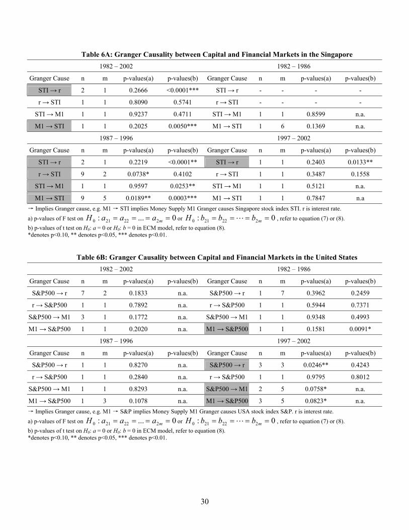
Table 6A: Granger Causality between Capital and Financial Markets in the Singapore 1982 – 2002 1982 – 1986

Granger Cause n m p-values(a) p-values(b) Granger Cause n m p-values(a) p-values(b)

STI → r 2 1 0.2666 <0.0001*** STI → r - - - -

r → STI 1 1 0.8090 0.5741 r → STI - - - -

STI → M1 1 1 0.9237 0.4711 STI → M1 1 1 0.8599 n.a.

M1 → STI 1 1 0.2025 0.0050*** M1 → STI 1 6 0.1369 n.a.

1987 – 1996 1997 – 2002

Granger Cause n m p-values(a) p-values(b) Granger Cause n m p-values(a) p-values(b)

STI → r 2 1 0.2219 <0.0001** STI → r 1 1 0.2403 0.0133**

r → STI 9 2 0.0738* 0.4102 r → STI 1 1 0.3487 0.1558

STI → M1 1 1 0.9597 0.0253** STI → M1 1 1 0.5121 n.a.

M1 → STI 9 5 0.0189** 0.0003*** M1 → STI 1 1 0.7847 n.a → Implies Granger cause, e.g. M1 → STI implies Money Supply M1 Granger causes Singapore stock index STI. r is interest rate. a) p-values of F test on 0...: 222210 ==== maaaH or 0: 222210 ==== mbbbH L , refer to equation (7) or (8). b) p-values of t test on H0: a = 0 or H0: b = 0 in ECM model, refer to equation (8). *denotes p<0.10, ** denotes p<0.05, *** denotes p<0.01.

Table 6B: Granger Causality between Capital and Financial Markets in the United States 1982 – 2002 1982 – 1986

Granger Cause n m p-values(a) p-values(b) Granger Cause n m p-values(a) p-values(b)

S&P500 → r 7 2 0.1833 n.a. S&P500 → r 1 7 0.3962 0.2459

r → S&P500 1 1 0.7892 n.a. r → S&P500 1 1 0.5944 0.7371

S&P500 → M1 3 1 0.1772 n.a. S&P500 → M1 1 1 0.9348 0.4993

M1 → S&P500 1 1 0.2020 n.a. M1 → S&P500 1 1 0.1581 0.0091*

1987 – 1996 1997 – 2002

Granger Cause n m p-values(a) p-values(b) Granger Cause n m p-values(a) p-values(b)

S&P500 → r 1 1 0.8270 n.a. S&P500 → r 3 3 0.0246** 0.4243

r → S&P500 1 1 0.2840 n.a. r → S&P500 1 1 0.9795 0.8012

S&P500 → M1 1 1 0.8293 n.a. S&P500 → M1 2 5 0.0758* n.a.

M1 → S&P500 1 3 0.1078 n.a. M1 → S&P500 3 5 0.0823* n.a. → Implies Granger cause, e.g. M1 → S&P implies Money Supply M1 Granger causes USA stock index S&P. r is interest rate. a) p-values of F test on 0...: 222210 ==== maaaH or 0: 222210 ==== mbbbH L , refer to equation (7) or (8). b) p-values of t test on H0: a = 0 or H0: b = 0 in ECM model, refer to equation (8). *denotes p<0.10, ** denotes p<0.05, *** denotes p<0.01.

30