Monetary policy and prudential regulation in a hybridAB-SFC model with heterogeneous expectations

Severin Reissl∗

Universita Cattolica del Sacro Cuore/Universitat Bielefeld

September 14, 2018

Abstract

This paper explores the joint effects of prudential regulation and monetary policy ina hybrid agent-based-stock-flow-consistent model featuring an agent-based bankingsector. Individual banks interact both with the aggregate portion of the model aswell as with each other, for instance through their decisions on interest-rate settingand on the inter-bank market. The model features a detailed depiction of pru-dential regulation and an active central bank which intervenes in money marketsto steer the inter-bank rate. Particular attention is paid to the modelling of bothtime and expectations formation. While the basic tick-length is one week, decisionsare assumed to take place at various frequencies within the agent-based portion ofthe model whilst in the aggregate portion, variables are assumed to evolve at dif-ferent speeds, incorporating differing decision-making horizons. Correspondingly,the horizons of expectations formation processes are modelled so as to match theadjustment speeds of forecasted variables. The model is calibrated to a determin-istic steady state and then simulated, producing a pattern of irregular short- andlonger-term fluctuations. Subsequent experiments indicate that whilst the modelis generally sensitive to the specification of expectations formation processes, animplementation of the canonical form of heterogeneous expectations with heuris-tic switching in the banking sector has very little discernible effect since it providesonly a minor improvement on standard adaptive expectations in terms of forecastingsuccess. This suggests that in certain macro settings, simple adaptive expectationsmay be a fairly robust heuristic. The presence of heterogeneous expectations hencedoes not noticeably affect the stability properties of the model and a combination ofmonetary and macro-prudential policy measures are necessary to dampen macroe-conomic fluctuations.

PRELIMINARY DRAFT - PLEASE DO NOT CITE

Keywords: Stock-flow consistent models, Agent-based models, Monetary policy, Pru-dential policy, Heterogeneous expectationsJEL-Classification: E12, E52, E58, E61, G28

∗Email: severindavid.reissl@unicatt.it

1 Introduction

This document aims to provide a compact overview of a hybrid agent-based stock-flow

consistent macro-model used to investigate the effects of heterogeneity in expectations for-

mation and the joint impacts of monetary policy and prudential regulation. The hybrid

model is constructed by fusing a macroeconomic stock-flow consistent model featuring

households, firms, non-bank financial firms, a government and a central bank with an

agent-based banking sector which interacts with the aggregate portions of the model

through various channels. The banking sector features a relatively detailed prudential

regulation regime modelled on the Basel III accord which makes it necessary for banks

to form expectations about the dynamics of their own balance sheets in order to meet

targets for prudential ratios which in turn feed back on their behaviour regarding interest

rate setting, credit rationing, equity issue and dividend policy. The goal is to investigate

the role of the expectations of banks and policy-makers and in particular their impact on

the effects of monetary and macro-prudential policies under different assumptions about

expectations formation processes.

This is very much a work in progress; the model is implemented and several simulations

have been carried out but some experiments and a thorough sensitivity analysis are still

ongoing and there are a few areas in which the model could be improved. Consequently

there does not yet exist a full write-up of the model and the simulation results. However

this document should serve to provide an overview of the model and the preliminary

results sufficient for a conference discussion.

This document is structured as follows: Section 2 gives a brief motivation for the research

and reviews some relevant literature. Section 3 outlines the structure of the model and

the most important behavioural assumptions. Section 4 discusses preliminary simulation

results and section 5 indicates planned future research and possible improvements to the

model.

2

2 Motivation and literature review

The purpose of this project is to combine insights from various strands of the literature

to advance research on agent-based stock-flow consistent (AB-SFC) models.

Over the last 10 to 15 years there have been substantial advances in the use of agent-based

models in macroeconomics, leading to the emergence of a number of different frameworks,

partly with different emphases, which have been applied to a variety of topics in macroe-

conomic research. Among others, these include the ‘Macroeconomics from the Bottom

Up’ (MBU) model (Delli Gatti et al., 2011), the various incarnations of the Eurace model

(Cincotti et al., 2010; Dawid et al., 2012), and the Keynes+Schumpeter model (Dosi

et al., 2006). The basic goal of all these frameworks is to provide an alternative way

to microfound macroeconomic models rooted in the complex adaptive systems paradigm,

emphasising agent interactions and emergent properties. Dawid and Delli Gatti (2018)

provide a comprehensive review of agent-based macroeconomics and compare the major

different frameworks in detail.

A by now fairly closely related strand of the literature which emerged out of the post-

Keynesian tradition in macroeconomic research is that of stock-flow consistent models

(see Godley and Lavoie (2007) who develop the approach as well as Caverzasi and Godin

(2015) and Nikiforos and Zezza (2017) for surveys). Stock-flow consistent models are typ-

ically aggregative (i.e. not ‘micro-founded’) and aim in particular at jointly modelling the

dynamics of national accounts variables and flow-of-funds variables within a fully consis-

tent accounting framework. This approach provides an important disciplining device and

consistency check in writing large-scale computational models and is essential in compre-

hensive depictions of real-financial interactions. By now, there exists a growing literature

which explicitly combines stock-flow consistent frameworks with agent-based modelling

in various ways (Dawid et al., 2012; Michell, 2014; Caiani et al., 2016; Seppecher, 2016).

The use of a stock-flow consistent framework may also partly help in overcoming the diffi-

culty of communicating and comparing different agent-based models since the accounting

3

relationships underlying any SFC model can be set out in a fairly compact fashion to give

a quick overview over the institutional structure of a given model. The present project

follows the trend of combining agent-based and SFC modelling techniques and in particu-

lar represents a contribution to the development of hybrid-aggregate-agent-based models

in which certain parts or sectors of the economy are modelled in an aggregate/structural

way or using representative agents whilst others (typically one sector) are disaggregated

and modelled using ABM. Examples of this include Assenza et al. (2007); Assenza and

Delli Gatti (2013) who apply this approach, using heterogeneous firms, to the Greenwald-

Stiglitz financial accelerator model Greenwald and Stiglitz (1993) and Michell (2014) who

uses an agent-based firm sector within an otherwise aggregate SFC framework to model

the ideas of Steindl Steindl (1952) regarding monopolisation and stagnation along with

Minsky’s (1986) trichotomy of hedge, speculative and Ponzi finance. The advantage of

such an approach is that important insights arising from agent heterogeneity and inter-

action can be gained from a hybrid model without the necessity of constructing a fully

agent-based framework, instead focussing on those sectors for which one wishes to exam-

ine the consequences of allowing for heterogeneity.

In the context of the present project, the emphasis is on introducing heterogeneity only

within the banking sector, which to the author’s knowledge has not been done thus far in

a hybrid AB-SFC model (indeed, even in the benchmark versions of many fully-fledged

ABM frameworks (e.g. in Delli Gatti et al. (2011) and Seppecher (2012)), it is assumed

for simplicity that there exists a unique/representative bank). The constructed model

is then used to discuss expectations formation under bounded rationality in the context

of financial regulation. The issues of bounded rationality, learning and (heterogeneous)

expectations formation are relatively long-standing components of the macroeconomic

literature, stemming from a dissatisfaction with the wide-ranging assumptions necessary

to sustain the concepts of rational choice and rational expectations in many contexts.

Bounded rationality is a broad concept, with contributions ranging from works such as

that of Sargent (1993) which arguably involves only minimal departures from full rational-

4

ity, via the heuristics and biases approach of (new) Behavioural Economics (Kahneman

and Tversky, 2000) to the ‘procedural/ecological’ rationality concepts of Simon (1982)

and Gigerenzer (2008) which aim to replace the traditional concept of perfect rationality

altogether. Regardless of one’s particular position on what (if anything) should replace

the assumption of full rationality, any departure from full rationality in the traditional

sense raises several thorny issues, especially how economic agents are envisioned to form

expectations if the absence of full rationality does not allow for the immediate application

of the rational expectations hypothesis, as will typically be the case in a computational

ABM. As explained in detail by Hommes (2013) any such departure quickly leads one

into the ‘wilderness of bounded rationality’, as there are countless different possible ways

to model imperfectly rational behavior and there is often no immediately obvious crite-

rion to prefer any one over all others. Several canonical ways of tackling this problem

have been proposed. Evans and Honkapohja (2001) develop the so-called e-learning ap-

proach whereby one can derive conditions under which agents, through attempting to

estimate model parameters, may be able to ‘learn’ the rational expectations equilibrium

of a model even in the absence of full rationality and perfect information. Hommes (2013)

is a book-length treatment of the idea, stemming from the seminal contribution of Brock

and Hommes (1997), that agents may switch between a number of different forecasting

strategies based on their relative performance, and possibly the cost of acquiring the nec-

essary information, which may or may not lead to convergence to a rational expectations

equilibrium.

While expectations formation, including under bounded rationality is thus widely dis-

cussed in the mainstream modelling literature, such considerations have had relatively

less impact in AB and SFC models in which simple adaptive or naive expectations are

typically assumed without much discussion. Thus for instance, Dosi et al. (2017) appears

to so far be the only paper explicitly applying structural heterogeneity of expectations and

e-learning in a macroeconomic ABM (although elements of the Bielefeld Eurace model

in which firms attempt to estimate demand elasticities are closely related, and other

5

approaches to modelling learning and adaptation from a major part of the agent-based

literature (e.g. Salle et al., 2012; Landini et al., 2014; Seppecher et al., 2016)). Further-

more, while in most ABMs, agents are by necessity boundedly rational and endowed with

imperfect information, specific modelling choices with regard to how agents form expec-

tations or which information they have access to are seldom discussed in detail, meaning

that there is much room to contribute to the existing literature.

The debates, following the global financial crisis, surrounding the appropriate conduct of

prudential regulation policy and its possible interactions with monetary policy (Galati and

Moessner, 2011; Barwell, 2013; Claessens et al., 2013; Freixas et al., 2015) provide a good

context in which to discuss the role of expectations in agent-based macroeconomic models.

As is well-known, expectations formation plays a key role in discussions of optimal policy

in mainstream models and there is a well-established body of knowledge regarding optimal

monetary policy (Gali, 2015) and departures from fully rational expectations are fairly

well-investigated (Branch and McGough, 2009; Massaro, 2013; Benchimol and Bounader,

2018). While there is also a large and growing literature on the conduct of (macro-)

prudential policy, this has not yet reached the same degree of sophistication, with debates

about fundamental issues such as instruments and targets still ongoing (Schoenmaker,

2014; Banque de France, 2014; Carre et al., 2015) and comparatively few examples of

macro-prudential policy in DSGE frameworks (Beau et al., 2012; Loisel, 2014; Angelini

et al., 2014). Nevertheless, the typical structure of a modern DSGE model makes it

obvious that also in the case of optimal prudential policy, expectations will play a crucial

role. Macro-prudential policy has also begun to gain importance in the ABM literature,

with several of the major frameworks being used to conduct policy experiments in financial

regulation (e.g. van der Hoog, 2015; van der Hoog and Dawid, 2015; Popoyan et al.,

2015; Salle and Seppecher, 2017; Krug, 2018). By contrast, there have been relatively few

treatments of this topic in pure aggregative SFC models (exceptions include Burgess et al.

(2016), Nikolaidi (2015) and Detzer (2016)), despite the distinct contributions of major

post-Keynesian authors to the theory of financial regulation. In all cases, the conduct of

6

prudential policy has not been linked explicitly to the treatment of boundedly rational

expectations. The present project hence aims to address a perceived shortcoming in the

AB(-SFC) literature regarding the treatment of expectations whilst at the same time

discussing a topic with high current policy relevance.

3 Model outline

The current section provides a compact overview of the model and its main behavioural

assumptions, beginning with its general sectoral stucture.

General structure

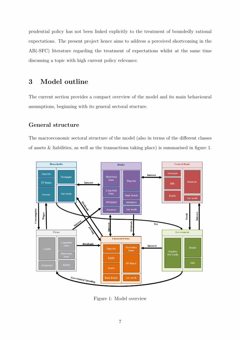
The macroeconomic sectoral structure of the model (also in terms of the different classes

of assets & liabilities, as well as the transactions taking place) is summarised in figure 1.

Figure 1: Model overview

7

The more traditional balance sheet and transactions flow matrices representing the ag-

gregate structure of the model (i.e. excluding transactions occurring within the banking

sector) are shown in tables 7 and 8 at the end of the document.

As can be seen, the model consists of 6 sectors, namely households, firms, non-bank fi-

nancial firms, the government, the central bank and the banks. The first five sectors are

modelled as aggregates without explicit micro-foundations whilst the banks are disaggre-

gated. In the present baseline, there exists an oligopolistic banking sector consisting of

12 banks which are structurally identical (i.e. they all hold the same types of assets and

liabilities) but may differ w.r.t. their decision-making and the precise composition of their

balance sheets. The following sub-sections provide an overview of the behaviours of the

individual sectors. The basic tick-length in simulations of this model is one week and it is

assumed that while all endogenous variables are computed on a weekly basis, some vari-

ables adjust more slowly than others (with a horizon of up to one year) and expectations

are formed over horizons consistent with the adjustment speed of the forecasted variable.

Households

Every week, the model computes a plan for household’s desired consumption over the

next month according to the Haig-Simons consumption function

(1) cd = α1 ∗ yde + α2 ∗ veh,

where yde is expected household disposable income over the next month and veh is their

expected wealth (both in real terms). The motivation of this rule, which is standard

in the SFC literature, bears similarity to many of the canonical ABM rules described

by Dawid and Delli Gatti (2018) and is also used in the benchmark AB-SFC of Caiani

et al. (2016), is that if disposable income is defined in a manner consistent with the Haig-

Simons definition of income, then this rule implicitly defines a target steady/stationary

state household wealth to disposable income ratio to which households adjust over time.1

1In a stationary state we must have vh = veh so that we need cd = yd(= yde = c), meaning that we

8

One variation on the usual assumption of constant consumption propensities (α1 and

α2) is that here they are assumed to depend on the (expected) real rate of return on

households’ financial assets according to a logistic function, meaning that the target ratio

of wealth to disposable income (and hence households’ saving) also becomes a function of

this return rate.

(2) α1 = αL1 +αU1 − αL1

1 + exp(σ1MPC ∗ rreh − σ2

MPC)

Both desired consumption and the ‘desired’ consumption propensities are computed every

period, but it is assumed, using an adaptive mechanism, that consumption adjusts more

quickly towards the desired level than do the consumption propensities, incorporating the

idea that some variables are more fast-moving than others.

The idea is the following: equation 1 is interpreted as giving an aggregate level of desired

consumption of all households represented by the modelled aggregate household sector.

At the same time, we assume that households on average update their consumption ev-

ery month, i.e. every 4 periods. Accordingly, we assume that every period (week), 1/4

of the gap between actual and desired consumption (which may of course itself change

from period to period) is closed. The same mechanism is applied to the consumption

propensities, but here we assume an updating frequency of 1 year. Inspired by the idea

of Calvo-pricing Calvo (1993), this principle is applied throughout the model, enabling us

to introduce a notion of asynchronous adaptive decision-making at differing frequencies

even in the case of sectors modelled as aggregates.

Households allocate their financial savings between bank deposits and shares in the non-

bank financial firms (these might be thought of as akin to shares in an MMMF) according

to a Brainard-Tobin portfolio equation (Brainard and Tobin, 1968; Kemp-Benedict and

Godin, 2017), which is standard in the SFC literature (though not in ABMs). In this case,

get vhyd = 1−α1

α2

9

deposits act as the buffer stock absorbing shocks and errors in expectations and portfolio

proportions are updated on a montly basis.

The final two important behavioural assumptions regarding households are their demand

for housing, and the dynamics of the wage rate. Households form a ‘notional’ demand for

houses according to

(3) Hnd = ρ0 + ρ1 ∗ V e

h, + ρ2 ∗ LTV − ρ3 ∗ rMe,

where LTV is the maximum loan-to-value ratio (which is constant in the baseline, but

can be endogenised at a later point) and rM is the average real interest rate charged

on mortgages. There is hence no ‘direct’ speculative element in housing demand (in the

sense that, for instance, (expected) house prices do not enter directly into the function),

although appreciation of the housing stock obviously has a positive impact on Vh. With

notional housing demand, the updating time horizon is assumed to be one quarter. Based

on the notional housing demand, households formulate a demand for mortgages based on

the LTV (which may or may not be fully satisfied), giving rise to an ‘effective’ demand

for houses. The supply of houses is determined by the assumption that in each period, a

constant fraction η of a constant total stock of houses in the model are up for sale. The

price of houses is then determined by market clearing.

Regarding wages, it is assumed that the (desired) nominal wage rate is determined by a

non-linear Phillips-curve-type equation of the form

(4) W = W−1 ∗ exp(β1 ∗ (ue − uwn ))

which is supposed to mimic the aggregate outcome of a wage-bargaining process. ue is

the expected rate of capacity utilisation whilst uwn is an endogenous, slowly adjusting

10

‘normal’ rate of capacity utilisation perceived by workers which might be thought of as

an endogenous quasi-NAIRU. A desired wage level according to the equation above is

determined every period, and the actual wage level adjusts slowly (horizon one year) to

this desired level.

Firms

Firms are assumed to plan their production of consumption goods weekly according to

an expectation of households’ consumption demand and the deviation of inventories from

a target level. By contrast, demand for investment goods and government consumption

are satisfied instantaneously (although we do assume that new capital goods do not come

online immediately, but rather only become available to boost capacity with a lag), i.e.

household consumption is the only source of inventory fluctuations. Firms use a Leontief

production function the coefficients of which are fixed throughout. This production func-

tion also defines a maximum of output which can be produced given the capital stock,

meaning that theoretically, there may be rationing of consumption demand in the model.

Moreover, the production function together with (planned) production imply a demand

for labour which is assumed to always be fully satisfied by households at the going wage

rate.

The target level of inventories is computed as

(5) Invt = γ1 ∗ ue ∗ yefc

where yefc is expected full capacity output and ue is expected capacity utilisation, both

computed over an annual horizon. Actual inventories (in the absence of fluctuations

caused by errors in the prediction of consumption demand) adjust to target inventories

11

according to

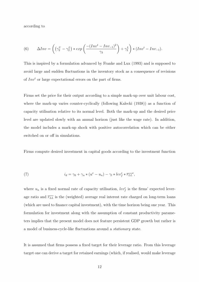
(6) ∆Inv =

((γU2 − γL2

)∗ exp

(−(Invt − Inv−1)2

γ3

)+ γL2

)∗ (Invt − Inv−1).

This is inspired by a formulation advanced by Franke and Lux (1993) and is supposed to

avoid large and sudden fluctuations in the inventory stock as a consequence of revisions

of Invt or large expectational errors on the part of firms.

Firms set the price for their output according to a simple mark-up over unit labour cost,

where the mark-up varies counter-cyclically (following Kalecki (1938)) as a function of

capacity utilisation relative to its normal level. Both the mark-up and the desired price

level are updated slowly with an annual horizon (just like the wage rate). In addition,

the model includes a mark-up shock with positive autocorrelation which can be either

switched on or off in simulations.

Firms compute desired investment in capital goods according to the investment function

(7) id = γ0 + γu ∗ (ue − un) − γl ∗ levef ∗ rLLe,

where un is a fixed normal rate of capacity utilisation, levef is the firms’ expected lever-

age ratio and rLL is the (weighted) average real interest rate charged on long-term loans

(which are used to finance capital investment), with the time horizon being one year. This

formulation for investment along with the assumption of constant productivity parame-

ters implies that the present model does not feature persistent GDP growth but rather is

a model of business-cycle-like fluctuations around a stationary state.

It is assumed that firms possess a fixed target for their leverage ratio. From this leverage

target one can derive a target for retained earnings (which, if realised, would make leverage

12

equal to its target) which in turn (given investment demand) determines firms’ demand for

long-term loans, and hence the combination of internal and external finance firms wish to

use to finance their investment. Short-term loans are used to finance inventories as well as

to make up for any financing shortfalls caused by errors in firms’ expectations. Dividend

payouts are determined by the difference between firms’ profit and target retained earnings

and adjust slowly, based on an annual horizon.

Non-bank financial firms

These entities may in essence be viewed as large portfolio equations. They hold govern-

ment bonds, the fixed stock of firm equity as well as ‘bank bonds’ (see below) and bank

deposits as their assets. Consequently, they receive a large share of the profit income

arising in the model (prior to distributing it to households), including from banks and

firms.

Financial firms’ demand for government bonds and bank bonds is determined by a To-

binesque portfolio equation (see Household section) with their holdings of bank deposits

acting as the buffer stock. Financial firms are financed by the shares eff they sell to

households as well as, if necessary, short-term loans from banks. Given the large range of

different assets they hold, they receive various flows of dividend and interest income, as

shown in figure 1 and table 8. It is assumed that they distribute all profits to households

(although these payments are updated slowly and hence reflect fluctuations in profits only

with a lag).

Government

The government collects taxes on household income (wages, interest and profits/dividends

accruing to households) at a fixed rate τ . It spends according to

(8) gd = (g0 + µ ∗ (un − ue)) ∗ exp(

1 − gby

gbyt

)µ2

.

13

gd is decided upon annually and over the following year, government spending gradually

adjusts to this desired value. gby is a moving average of the government debt to income

ratio and gbyt is the corresponding target. Deficits are covered by issuance of government

bonds on a rolling basis. Government bonds are offered in the first instance to financial

firms, and the government attempts to generate sufficient demand for bonds by managing

the government bond interest rate to keep it close to its market-clearing level derived from

financial firms’ portfolio choice.

Central Bank

Every month (again as with government spending, this is a discrete decision), the central

bank sets a nominal deposit rate according to a Taylor-type pure inflation-targeting rule:

(9) rcb,d = r0 + πe + φπ ∗ (πe − πt).

Its lending rate is given by a constant mark-up over this rate, giving rise to a corridor sys-

tem. In addition, we suppose that the central bank has in mind a target interbank rate in

the middle of this corridor and continuously carries out open-market operations in order

to steer the level of central bank reserves to a level consistent with this target. It does

so by purchasing and selling government bonds from/to the financial firms (for simplicity

we assume that the financial firms are always willing to enter into such transactions). If

necessary, the central bank also acts as a lender of last resort to the government. All

central bank profits are transferred to the government (and all losses are reimbursed by

the government).

In the present version of the model, the central bank is always able to perfectly target the

correct level of reserves, meaning that banks are never ‘in the Bank’ to acquire advances.

However there is a possibility of introducing a stochastic term (which might be thought of

as representing noise in the CB’s information about the required level of reserves) which

induces the possibility of temporary aggregate reserve shortfalls or surpluses, which in

turn also makes interactions on the interbank market more interesting.

14

In addition, the central bank is thought of as the macro-prudential policy-maker in the

model. At present, the model includes four principal prudential policy levers, namely

the capital adequacy ratio, the stable funding ratio, the liquidity coverage ratio and a

maximum loan-to-value ratio on mortgages, all applying to banks. In the baseline, the

targets for all these regulatory ratios are assumed constant.

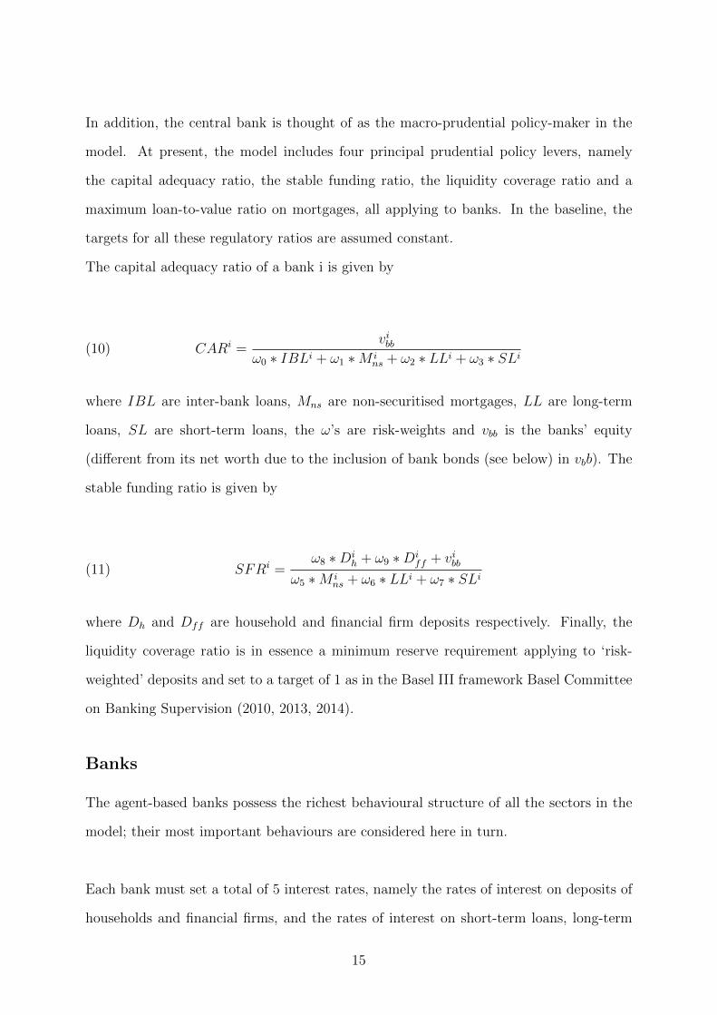
The capital adequacy ratio of a bank i is given by

(10) CARi =vibb

ω0 ∗ IBLi + ω1 ∗M ins + ω2 ∗ LLi + ω3 ∗ SLi

where IBL are inter-bank loans, Mns are non-securitised mortgages, LL are long-term

loans, SL are short-term loans, the ω’s are risk-weights and vbb is the banks’ equity

(different from its net worth due to the inclusion of bank bonds (see below) in vbb). The

stable funding ratio is given by

(11) SFRi =ω8 ∗Di

h + ω9 ∗Diff + vibb

ω5 ∗M ins + ω6 ∗ LLi + ω7 ∗ SLi

where Dh and Dff are household and financial firm deposits respectively. Finally, the

liquidity coverage ratio is in essence a minimum reserve requirement applying to ‘risk-

weighted’ deposits and set to a target of 1 as in the Basel III framework Basel Committee

on Banking Supervision (2010, 2013, 2014).

Banks

The agent-based banks possess the richest behavioural structure of all the sectors in the

model; their most important behaviours are considered here in turn.

Each bank must set a total of 5 interest rates, namely the rates of interest on deposits of

households and financial firms, and the rates of interest on short-term loans, long-term

15

loans and mortgages. It is assumed that each period, a random sample of banks is drawn

(such that on average, each bank is drawn once every 4 ticks) and these are allowed to

adjust their interest rate in a given period (meaning that on average, each bank can adjust

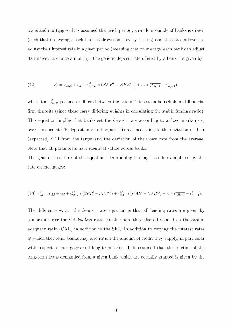
its interest rate once a month). The generic deposit rate offered by a bank i is given by

(12) rid = rcb,d + εd + εdSFR ∗ (SFRt − SFRe,i) + εr ∗ (rd,−1 − rid,−1),

where the εdSFR parameter differs between the rate of interest on household and financial

firm deposits (since these carry differing weights in calculating the stable funding ratio).

This equation implies that banks set the deposit rate according to a fixed mark-up εd

over the current CB deposit rate and adjust this rate according to the deviation of their

(expected) SFR from the target and the deviation of their own rate from the average.

Note that all parameters have identical values across banks.

The general structure of the equations determining lending rates is exemplified by the

rate on mortgages:

(13) riM = rcb,l + εM + εMSFR ∗ (SFRt − SFRe,i) + εMCAR ∗ (CARt − CARe,i) + εr ∗ (rM,−1 − riM,−1).

The difference w.r.t. the deposit rate equation is that all lending rates are given by

a mark-up over the CB lending rate. Furthermore they also all depend on the capital

adequacy ratio (CAR) in addition to the SFR. In addition to varying the interest rates

at which they lend, banks may also ration the amount of credit they supply, in particular

with respect to mortgages and long-term loans. It is assumed that the fraction of the

long-term loans demanded from a given bank which are actually granted is given by the

16

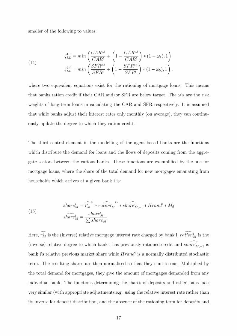
smaller of the following to values:

ξ1,iLL = min

(CARe,i

CARt+

(1 − CARe,i

CARt

)∗ (1 − ω1), 1

)ξ2,iLL = min

(SFRe,i

SFRt+

(1 − SFRe,i

SFRt

)∗ (1 − ω5), 1

),

(14)

where two equivalent equations exist for the rationing of mortgage loans. This means

that banks ration credit if their CAR and/or SFR are below target. The ω’s are the risk

weights of long-term loans in calculating the CAR and SFR respectively. It is assumed

that while banks adjust their interest rates only monthly (on average), they can continu-

ously update the degree to which they ration credit.

The third central element in the modelling of the agent-based banks are the functions

which distribute the demand for loans and the flows of deposits coming from the aggre-

gate sectors between the various banks. These functions are exemplified by the one for

mortgage loans, where the share of the total demand for new mortgages emanating from

households which arrives at a given bank i is:

shareiM = riMι1∗ rationiM

ι2∗ shareiM,−1 ∗Hrand

i ∗Md

˜shareiM =shareiM∑shareM

(15)

Here, riM is the (inverse) relative mortgage interest rate charged by bank i, rationiM is the

(inverse) relative degree to which bank i has previously rationed credit and shareiM,−1 is

bank i’s relative previous market share while Hrandi is a normally distributed stochastic

term. The resulting shares are then normalised so that they sum to one. Multiplied by

the total demand for mortgages, they give the amount of mortgages demanded from any

individual bank. The functions determining the shares of deposits and other loans look

very similar (with appropriate adjustments e.g. using the relative interest rate rather than

its inverse for deposit distribution, and the absence of the rationing term for deposits and

17

short-term loans).

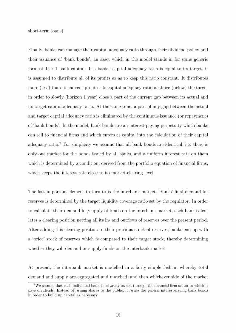
Finally, banks can manage their capital adequacy ratio through their dividend policy and

their issuance of ‘bank bonds’, an asset which in the model stands in for some generic

form of Tier 1 bank capital. If a banks’ capital adequacy ratio is equal to its target, it

is assumed to distribute all of its profits so as to keep this ratio constant. It distributes

more (less) than its current profit if its capital adequacy ratio is above (below) the target

in order to slowly (horizon 1 year) close a part of the current gap between its actual and

its target capital adequacy ratio. At the same time, a part of any gap between the actual

and target captial adequacy ratio is eliminated by the continuous issuance (or repayment)

of ‘bank bonds’. In the model, bank bonds are an interest-paying perpetuity which banks

can sell to financial firms and which enters as capital into the calculation of their capital

adequacy ratio.2 For simplicity we assume that all bank bonds are identical, i.e. there is

only one market for the bonds issued by all banks, and a uniform interest rate on them

which is determined by a condition, derived from the portfolio equation of financial firms,

which keeps the interest rate close to its market-clearing level.

The last important element to turn to is the interbank market. Banks’ final demand for

reserves is determined by the target liquidity coverage ratio set by the regulator. In order

to calculate their demand for/supply of funds on the interbank market, each bank calcu-

lates a clearing position netting all its in- and outflows of reserves over the present period.

After adding this clearing position to their previous stock of reserves, banks end up with

a ‘prior’ stock of reserves which is compared to their target stock, thereby determining

whether they will demand or supply funds on the interbank market.

At present, the interbank market is modelled in a fairly simple fashion whereby total

demand and supply are aggregated and matched, and then whichever side of the market

2We assume that each individual bank is privately owned through the financial firm sector to which itpays dividends. Instead of issuing shares to the public, it issues the generic interest-paying bank bondsin order to build up capital as necessary.

18

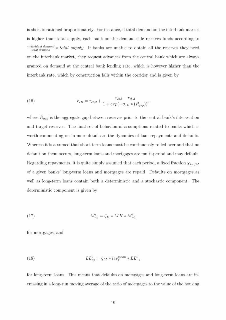
is short is rationed proportionately. For instance, if total demand on the interbank market

is higher than total supply, each bank on the demand side receives funds according to

individual demandtotal demand

∗ total supply. If banks are unable to obtain all the reserves they need

on the interbank market, they request advances from the central bank which are always

granted on demand at the central bank lending rate, which is however higher than the

interbank rate, which by construction falls within the corridor and is given by

(16) rIB = rcb,d +rcb,l − rcb,d

1 + exp(−σIB ∗ (Rgap)),

where Rgap is the aggregate gap between reserves prior to the central bank’s intervention

and target reserves. The final set of behavioural assumptions related to banks which is

worth commenting on in more detail are the dynamics of loan repayments and defaults.

Whereas it is assumed that short-term loans must be continuously rolled over and that no

default on them occurs, long-term loans and mortgages are multi-period and may default.

Regarding repayments, it is quite simply assumed that each period, a fixed fraction χLL/M

of a given banks’ long-term loans and mortgages are repaid. Defaults on mortgages as

well as long-term loans contain both a deterministic and a stochastic component. The

deterministic component is given by

(17) M inp = ζM ∗MH ∗M i

−1

for mortgages, and

(18) LLinp = ζLL ∗ levmeanf ∗ LLi−1

for long-term loans. This means that defaults on mortgages and long-term loans are in-

creasing in a long-run moving average of the ratio of mortgages to the value of the housing

19

stock (MH) and firms’ leverage ratio respectively. In addition, each default equation also

contains a normally distributed stochastic component, which is added on to the deter-

ministic component.

At present, the model does not contain a bankruptcy mechanism for banks which for the

moment does not represent a problem since no bank has so far gone bankrupt in any

simulation.

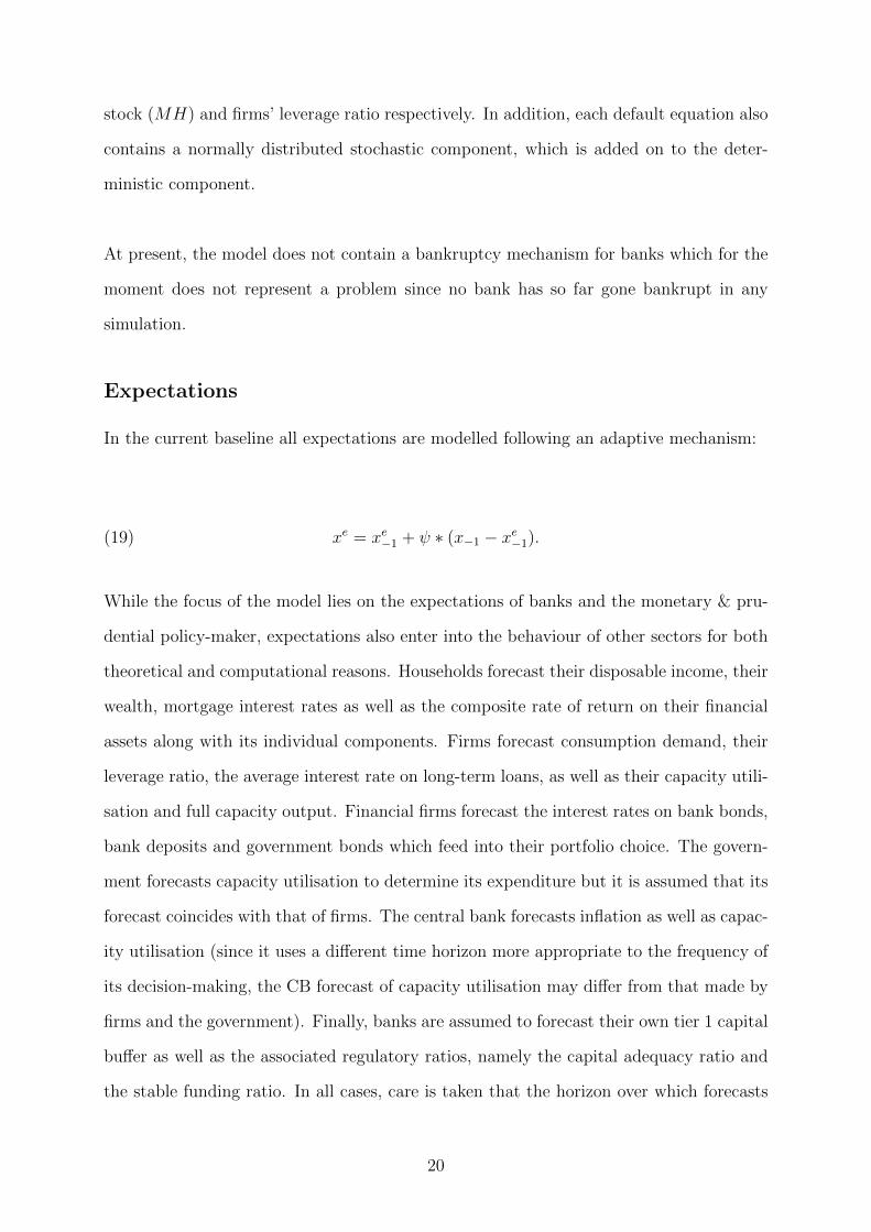
Expectations

In the current baseline all expectations are modelled following an adaptive mechanism:

(19) xe = xe−1 + ψ ∗ (x−1 − xe−1).

While the focus of the model lies on the expectations of banks and the monetary & pru-

dential policy-maker, expectations also enter into the behaviour of other sectors for both

theoretical and computational reasons. Households forecast their disposable income, their

wealth, mortgage interest rates as well as the composite rate of return on their financial

assets along with its individual components. Firms forecast consumption demand, their

leverage ratio, the average interest rate on long-term loans, as well as their capacity utili-

sation and full capacity output. Financial firms forecast the interest rates on bank bonds,

bank deposits and government bonds which feed into their portfolio choice. The govern-

ment forecasts capacity utilisation to determine its expenditure but it is assumed that its

forecast coincides with that of firms. The central bank forecasts inflation as well as capac-

ity utilisation (since it uses a different time horizon more appropriate to the frequency of

its decision-making, the CB forecast of capacity utilisation may differ from that made by

firms and the government). Finally, banks are assumed to forecast their own tier 1 capital

buffer as well as the associated regulatory ratios, namely the capital adequacy ratio and

the stable funding ratio. In all cases, care is taken that the horizon over which forecasts

20

are made is consistent with the horizon over which decisions involving these expected

values are made.

The first experiment, reported below, consists in replacing the adaptive expectations

mechanism in the banking sector with the model of heterogeneous expectations formation

and heuristic switching first proposed by Brock and Hommes (1997); more specifically we

use the version presented in Anufriev and Hommes (2012) where it is assumed that agents

can switch between four different specifications for expected variables given by

xe1 = xe1−1 + ψad ∗ (x−1 − xe1−1)

xe2 = x−1 + ψtf1 ∗ (x−1 − x−2)

xe3 = x−1 + ψtf2 ∗ (x−1 − x−2)

xe4 = ψaa ∗ (x−1 + x−1) + (x−1 − x−2).

(20)

The first rule is the same adaptive one used in the baseline, which is now augmented with

two trend-following rules (one weak and one strong) and an ‘anchoring and adjustment’

mechanism in which the anchor is the moving average of x. Agents switch between these

four mechanisms based on a fitness function calculated using the error between expected

values and realisations of the forecasted variables as detailed in Anufriev and Hommes

(2012).

4 Preliminary simulation results

The model is calibrated to a deterministic stationary state through imposing realis-

tic stationary-state values for certain variables and ratios (e.g. capacity utilisation,

government-debt-to-GDP, investment-to-income, government-consumption-to-income, capital-

to-full-capacity-output,...), and using the SFC-structure of the model to reduce the num-

ber of degrees of freedom. This procedure greatly reduces the number of ‘free’ parameters

the value of which is independent of the initial stationary state and on which the sensitiv-

21

ity analysis will focus. For the banking sector, which in the baseline contains 12 banks,

a heterogeneous initialisation is used to begin the simulation with a size-distribution of

banks similar to that found in economies with oligopolistic banking sectors such as that

of the UK. The baseline simulation is conducted using 100 Monte Carlo repetitions, with

stochastic elements emanating from the default process, the distribution of aggregate

flows of loan demand and deposits between banks, the mark-up shock and noise in the

central bank’s perceived target level of reserves. After discarding a transient, the baseline

simulates the behaviour of the model for 1200 periods, corresponding to 25 years (it is

assumed that one year is made up of 48 weeks).

Starting from the deterministic stationary state, the random elements present in the

simulation are sufficient to make the economy diverge from the stationary state and

converge to an irregular cyclical movement featuring short-term fluctuations primarily

driven by investment and longer cycles driven by consumption expenditure. It should

be noted that the mark-up shocks are not strictly required for this outcome. Stochastic

elements at the level of the individual banks alone are sufficient to induce convergence

a cyclical movement at the macroeconomic level, although the presence of macro-level

shocks does speed up this convergence. Figures 2 to 7 provide an overview of the aggregate

results of a representative single run of the model. The persistent cycles are fundamentally

driven by the interactions of the non-linearities present in the aggregate structure of the

model, with the slow-moving consumption propensities, together with wage dynamics and

the component of capital investment responding to trends in capacity utilisation giving

rise to long cycles in consumption and the interaction between the central banks’ interest

rate policy, banks’ interest rate setting and credit rationing and the influence thereof on

firms’ investment decision producing shorter-run fluctuations in aggregate income. The

central bank appears to be relatively successful at keeping the rate of inflation close to its

target, here assumed to be zero.

22

Figure 2: Real GDP and components for a single run

Figure 3: Capacity utilisation for a single run

23

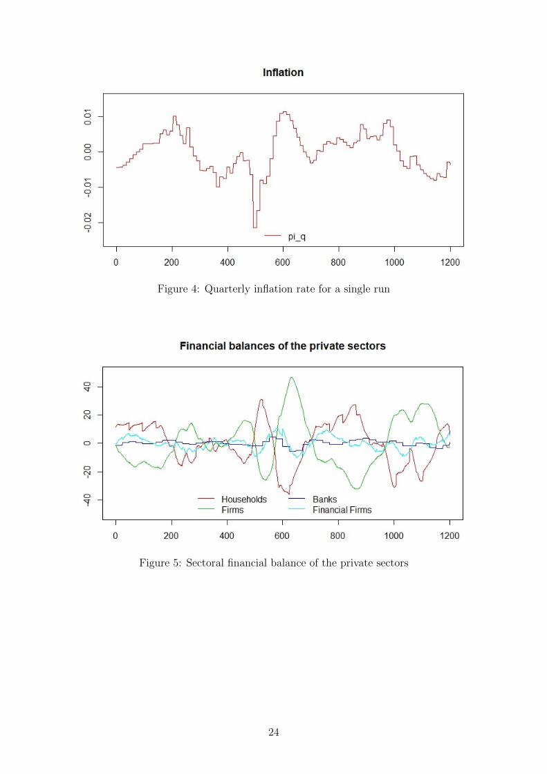
Figure 4: Quarterly inflation rate for a single run

Figure 5: Sectoral financial balance of the private sectors

24

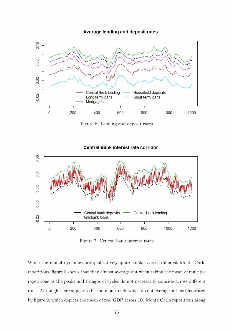
Figure 6: Lending and deposit rates

Figure 7: Central bank interest rates

While the model dynamics are qualitatively quite similar across different Monte Carlo

repetitions, figure 8 shows that they almost average out when taking the mean of multiple

repetitions as the peaks and troughs of cycles do not necessarily coincide across different

runs. Although there appear to be common trends which do not average out, as illustrated

by figure 9, which depicts the mean of real GDP across 100 Monte Carlo repetitions along

25

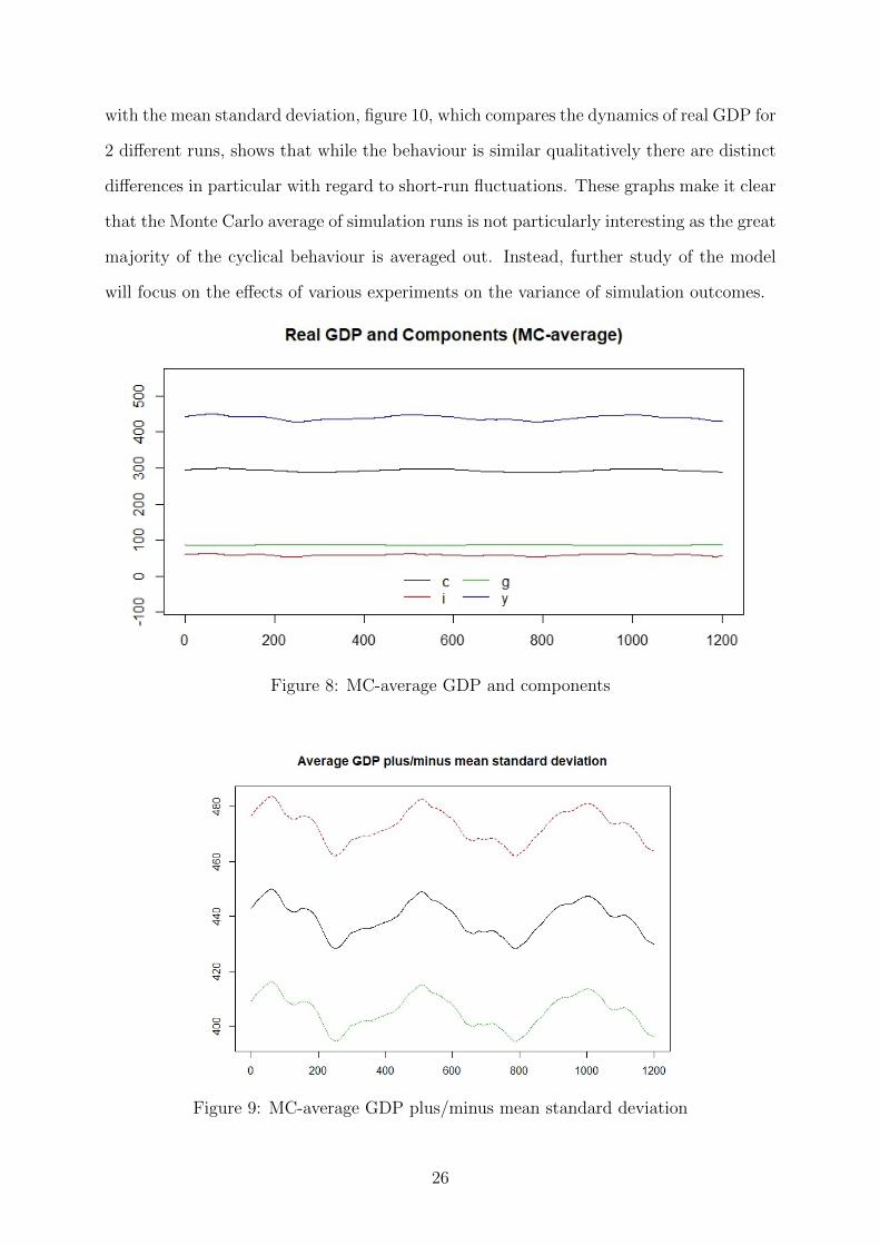
with the mean standard deviation, figure 10, which compares the dynamics of real GDP for

2 different runs, shows that while the behaviour is similar qualitatively there are distinct

differences in particular with regard to short-run fluctuations. These graphs make it clear

that the Monte Carlo average of simulation runs is not particularly interesting as the great

majority of the cyclical behaviour is averaged out. Instead, further study of the model

will focus on the effects of various experiments on the variance of simulation outcomes.

Figure 8: MC-average GDP and components

Figure 9: MC-average GDP plus/minus mean standard deviation

26

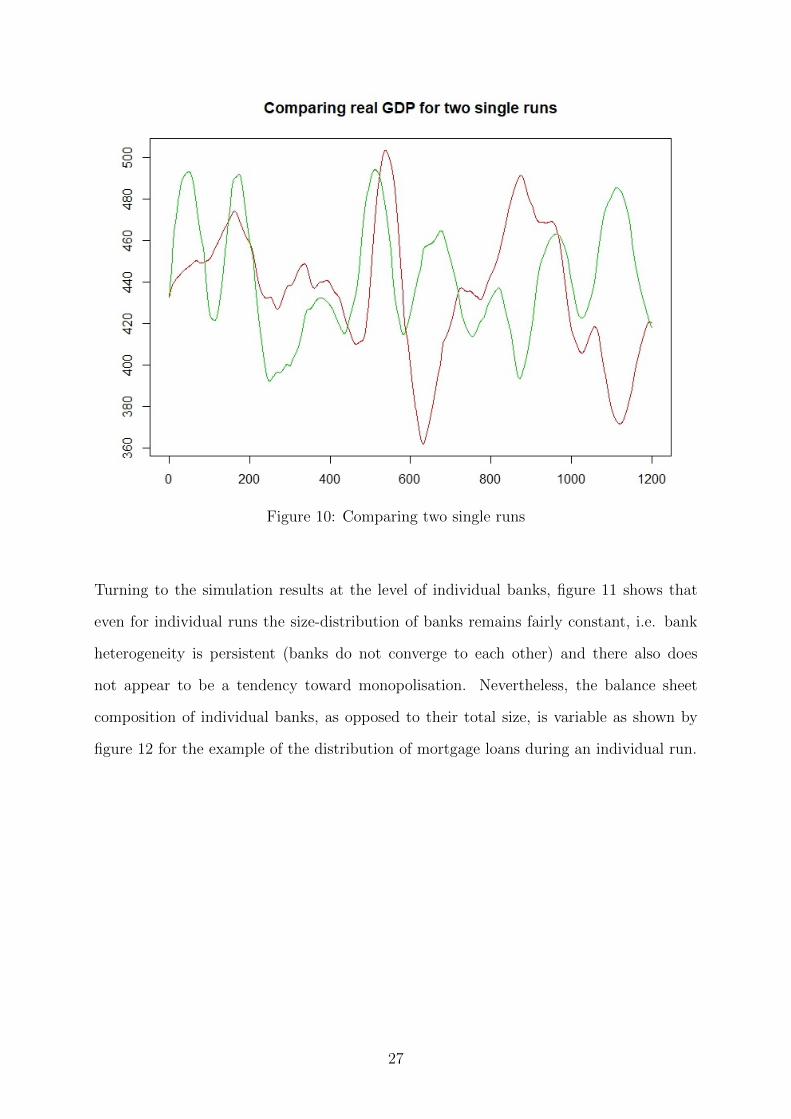
Figure 10: Comparing two single runs

Turning to the simulation results at the level of individual banks, figure 11 shows that

even for individual runs the size-distribution of banks remains fairly constant, i.e. bank

heterogeneity is persistent (banks do not converge to each other) and there also does

not appear to be a tendency toward monopolisation. Nevertheless, the balance sheet

composition of individual banks, as opposed to their total size, is variable as shown by

figure 12 for the example of the distribution of mortgage loans during an individual run.

27

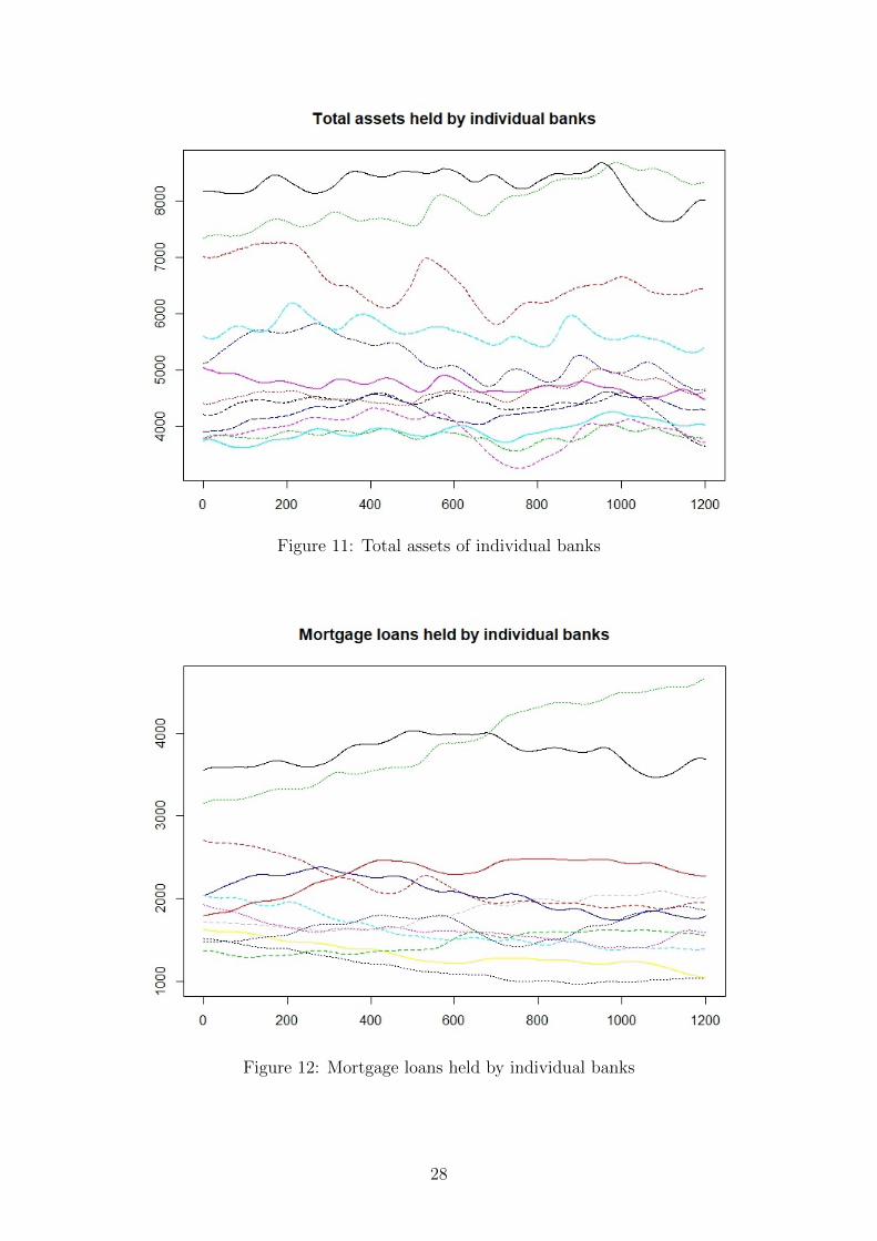
Figure 11: Total assets of individual banks

Figure 12: Mortgage loans held by individual banks

28

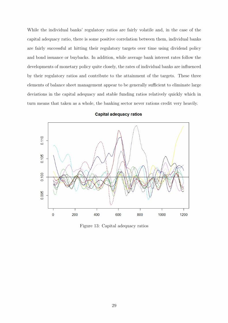
While the individual banks’ regulatory ratios are fairly volatile and, in the case of the

capital adequacy ratio, there is some positive correlation between them, individual banks

are fairly successful at hitting their regulatory targets over time using dividend policy

and bond issuance or buybacks. In addition, while average bank interest rates follow the

developments of monetary policy quite closely, the rates of individual banks are influenced

by their regulatory ratios and contribute to the attainment of the targets. These three

elements of balance sheet management appear to be generally sufficient to eliminate large

deviations in the capital adequacy and stable funding ratios relatively quickly which in

turn means that taken as a whole, the banking sector never rations credit very heavily.

Figure 13: Capital adequacy ratios

29

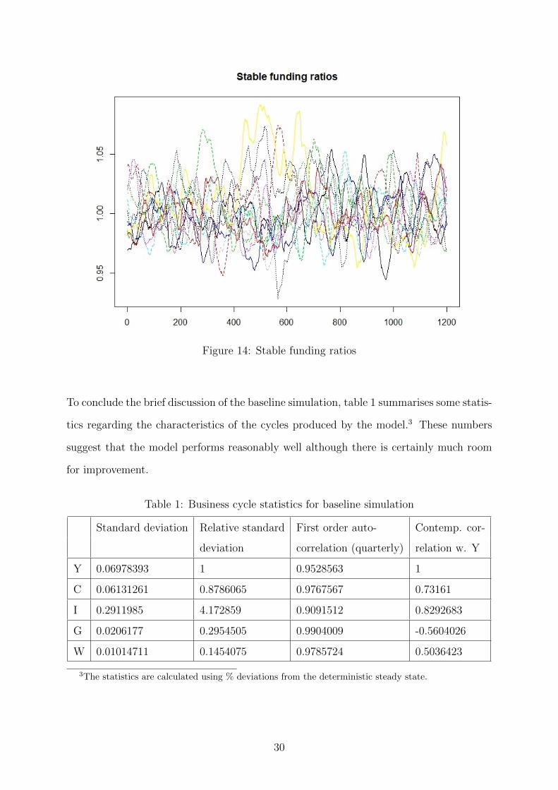
Figure 14: Stable funding ratios

To conclude the brief discussion of the baseline simulation, table 1 summarises some statis-

tics regarding the characteristics of the cycles produced by the model.3 These numbers

suggest that the model performs reasonably well although there is certainly much room

for improvement.

Table 1: Business cycle statistics for baseline simulation

Standard deviation Relative standard First order auto- Contemp. cor-

deviation correlation (quarterly) relation w. Y

Y 0.06978393 1 0.9528563 1

C 0.06131261 0.8786065 0.9767567 0.73161

I 0.2911985 4.172859 0.9091512 0.8292683

G 0.0206177 0.2954505 0.9904009 -0.5604026

W 0.01014711 0.1454075 0.9785724 0.5036423

3The statistics are calculated using % deviations from the deterministic steady state.

30

Experiments

Given the importance of banks’ balance sheet management for the observed model dynam-

ics, a straightforward experiment to carry out is to replace banks’ adaptive expectations

formation process with the heterogeneous expectations and heuristic switching mechanism

outlined in the previous section. As was explained in the model description, banks’ ex-

pectations about their capital buffer, their capital adequacy ratio and their stable funding

ratio feed into most aspects of their decision-making. Interestingly, however, an imple-

mentation of the mechanism described in Anufriev and Hommes (2012) in the present

version of the model appears to have little qualitative effect on simulation results. Banks

do indeed switch between different heuristics and after the transient during which fre-

quent switching between all four heuristics occurs, the strong and weak trend-following

rules become dominant. However, in the present model which is stationary and exhibits

persistent cycles, simple adaptive expectations by themselves turn out to be a fairly de-

cent forecasting heuristic upon which heterogeneous expectations provide only a slight

improvement. Table 2 shows improvements in the mean forecast error for all variables

forecasted by the banks, but also demonstrates that on average errors are small even

under adaptive expectations. Table 3 shows perhaps more clearly that heterogeneous

expectations do indeed significantly outperform simple adaptive expectations in that the

former lead to far smaller standard deviations in forecast errors.

Table 2: Mean forecast errors

CAR SFR Capital Buffer

Baseline 5.268677e-07 -1.790212e-06 0.002958

Het. Expectations -1.05351e-07 -1.278779e-06 -0.000584927

31

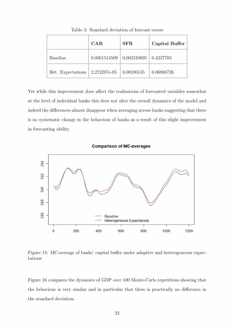
Table 3: Standard deviation of forecast errors

CAR SFR Capital Buffer

Baseline 0.0001514509 0.002310695 0.4227703

Het. Expectations 2.272287e-05 0.00100135 0.06806726

Yet while this improvement does affect the realisations of forecasted variables somewhat

at the level of individual banks this does not alter the overall dynamics of the model and

indeed the differences almost disappear when averaging across banks suggesting that there

is no systematic change in the behaviour of banks as a result of this slight improvement

in forecasting ability.

Figure 15: MC-average of banks’ capital buffer under adaptive and heterogeneous expec-tations

Figure 16 compares the dynamics of GDP over 100 Monte-Carlo repetitions showing that

the behaviour is very similar and in particular that there is practically no difference in

the standard deviation.

32

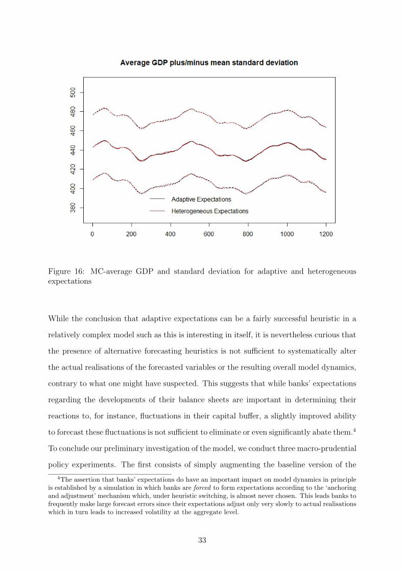
Figure 16: MC-average GDP and standard deviation for adaptive and heterogeneousexpectations

While the conclusion that adaptive expectations can be a fairly successful heuristic in a

relatively complex model such as this is interesting in itself, it is nevertheless curious that

the presence of alternative forecasting heuristics is not sufficient to systematically alter

the actual realisations of the forecasted variables or the resulting overall model dynamics,

contrary to what one might have suspected. This suggests that while banks’ expectations

regarding the developments of their balance sheets are important in determining their

reactions to, for instance, fluctuations in their capital buffer, a slightly improved ability

to forecast these fluctuations is not sufficient to eliminate or even significantly abate them.4

To conclude our preliminary investigation of the model, we conduct three macro-prudential

policy experiments. The first consists of simply augmenting the baseline version of the

4The assertion that banks’ expectations do have an important impact on model dynamics in principleis established by a simulation in which banks are forced to form expectations according to the ‘anchoringand adjustment’ mechanism which, under heuristic switching, is almost never chosen. This leads banks tofrequently make large forecast errors since their expectations adjust only very slowly to actual realisationswhich in turn leads to increased volatility at the aggregate level.

33

model with an endogenous target for the capital adequacy ratio, as opposed to the fixed

one present in the simulations shown above. The endogenous target is given by

(21) CARt = CARt0 + 0.5 ∗ cr,

where cr is the annualised growth rate of bank credit to the private non-financial sectors

and CARt0 is an exogenous intercept equal to the fixed target in the baseline. It is as-

sumed that the central bank revises the target CAR once a month, concurrently with its

monetary policy decision, based on the average of cr during the previous month.

The experiment is carried out using 25 MC repetitions. Comparing the MC-averages of

GDP with those of the baseline model for the same number of repetitions with identical

seeds it can clearly be seen that the endogenous CAR contributes to stabilising the ag-

gregate dynamics by dampening longer-term fluctuations, albeit introducing some very

minor short-term fluctuations caused by frequent adjustments of the target CAR.

Figure 17: MC-average GDP for baseline and endogenous CAR

34

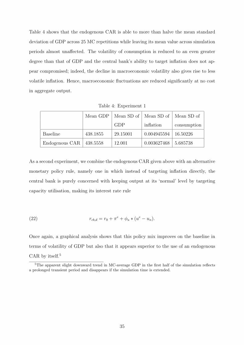
Table 4 shows that the endogenous CAR is able to more than halve the mean standard

deviation of GDP across 25 MC repetitions while leaving its mean value across simulation

periods almost unaffected. The volatility of consumption is reduced to an even greater

degree than that of GDP and the central bank’s ability to target inflation does not ap-

pear compromised; indeed, the decline in macroeconomic volatility also gives rise to less

volatile inflation. Hence, macroeconomic fluctuations are reduced significantly at no cost

in aggregate output.

Table 4: Experiment 1

Mean GDP Mean SD of Mean SD of Mean SD of

GDP inflation consumption

Baseline 438.1855 29.15001 0.004945594 16.50226

Endogenous CAR 438.5558 12.001 0.003627468 5.685738

As a second experiment, we combine the endogenous CAR given above with an alternative

monetary policy rule, namely one in which instead of targeting inflation directly, the

central bank is purely concerned with keeping output at its ‘normal’ level by targeting

capacity utilisation, making its interest rate rule

(22) rcb,d = r0 + πe + φu ∗ (ue − un).

Once again, a graphical analysis shows that this policy mix improves on the baseline in

terms of volatility of GDP but also that it appears superior to the use of an endogenous

CAR by itself.5

5The apparent slight downward trend in MC-average GDP in the first half of the simulation reflectsa prolonged transient period and disappears if the simulation time is extended.

35

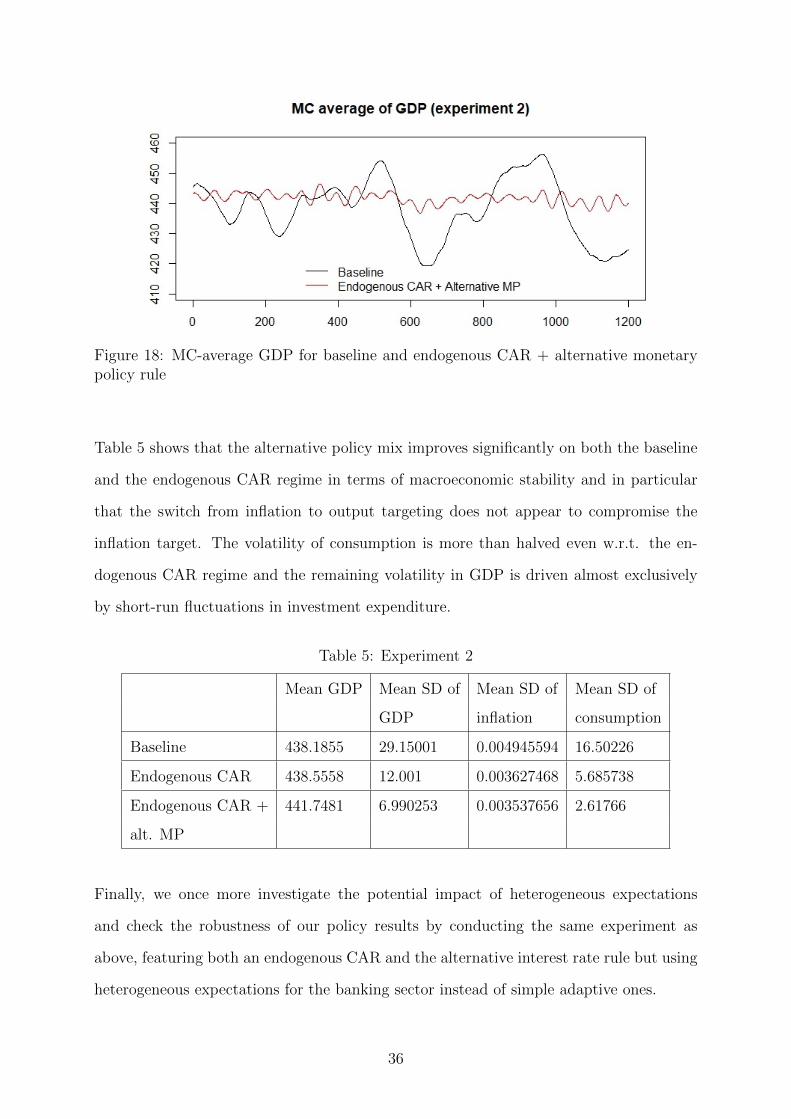
Figure 18: MC-average GDP for baseline and endogenous CAR + alternative monetarypolicy rule

Table 5 shows that the alternative policy mix improves significantly on both the baseline

and the endogenous CAR regime in terms of macroeconomic stability and in particular

that the switch from inflation to output targeting does not appear to compromise the

inflation target. The volatility of consumption is more than halved even w.r.t. the en-

dogenous CAR regime and the remaining volatility in GDP is driven almost exclusively

by short-run fluctuations in investment expenditure.

Table 5: Experiment 2

Mean GDP Mean SD of Mean SD of Mean SD of

GDP inflation consumption

Baseline 438.1855 29.15001 0.004945594 16.50226

Endogenous CAR 438.5558 12.001 0.003627468 5.685738

Endogenous CAR + 441.7481 6.990253 0.003537656 2.61766

alt. MP

Finally, we once more investigate the potential impact of heterogeneous expectations

and check the robustness of our policy results by conducting the same experiment as

above, featuring both an endogenous CAR and the alternative interest rate rule but using

heterogeneous expectations for the banking sector instead of simple adaptive ones.

36

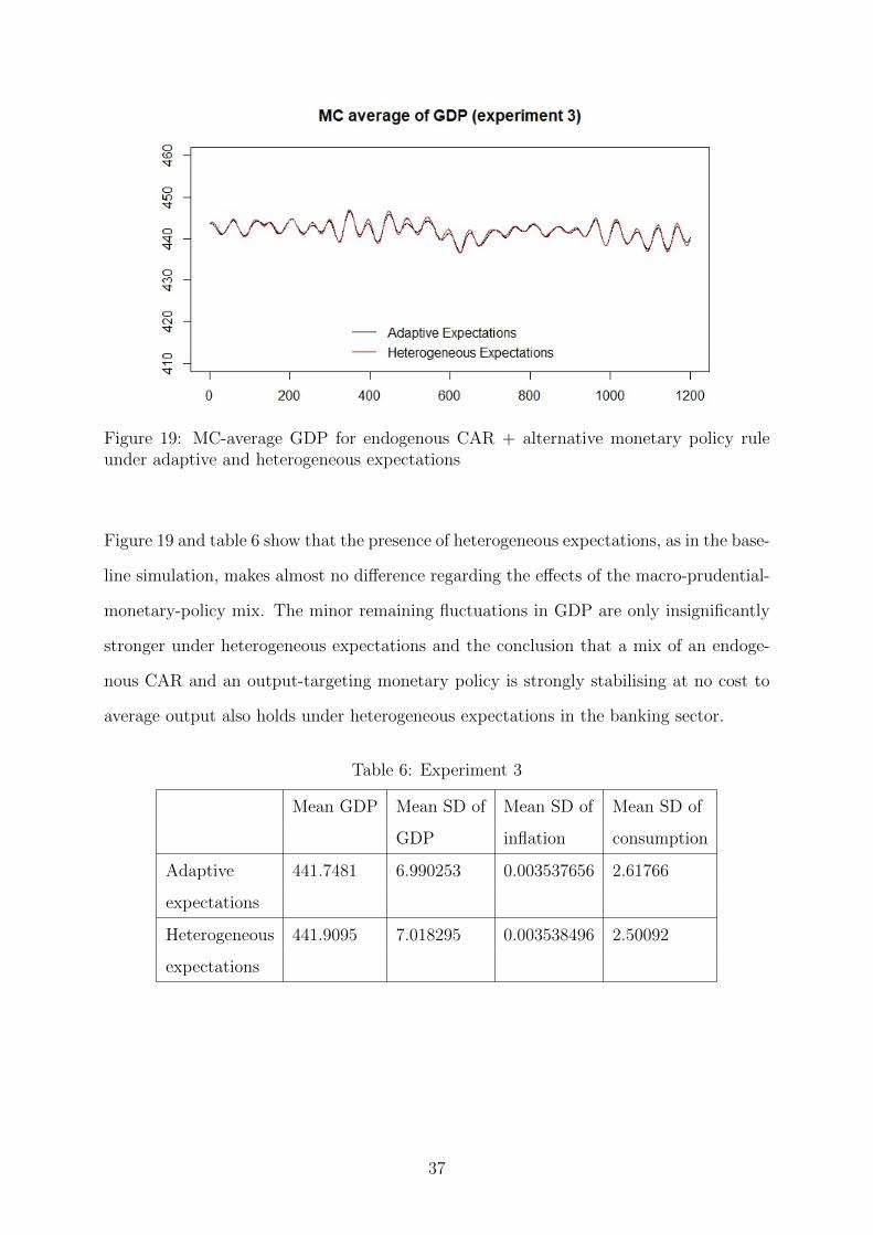
Figure 19: MC-average GDP for endogenous CAR + alternative monetary policy ruleunder adaptive and heterogeneous expectations

Figure 19 and table 6 show that the presence of heterogeneous expectations, as in the base-

line simulation, makes almost no difference regarding the effects of the macro-prudential-

monetary-policy mix. The minor remaining fluctuations in GDP are only insignificantly

stronger under heterogeneous expectations and the conclusion that a mix of an endoge-

nous CAR and an output-targeting monetary policy is strongly stabilising at no cost to

average output also holds under heterogeneous expectations in the banking sector.

Table 6: Experiment 3

Mean GDP Mean SD of Mean SD of Mean SD of

GDP inflation consumption

Adaptive 441.7481 6.990253 0.003537656 2.61766

expectations

Heterogeneous 441.9095 7.018295 0.003538496 2.50092

expectations

37

5 Future research

At present, a thorough sensitivity analysis of the baseline using latin hypercube sampling

to sample the parameter space is still to be completed. In addition, the model still

allows for a range of further policy experiments. More broadly there are several places

in which the model could be improved, particularly with regard to the behaviour of the

banking sector. At present banks’ behaviour largely revolves around attempts to meet

their various regularly constraints and there is little explicitly profit-oriented behaviour.6

Improvements on this could be made by having banks calculating the expected revenue

and cost of making a given amount of loans (including the expectation of default which at

present only enters indirectly through banks’ forecast of their capital buffer) and paying

closer attention to their funding cost, including that emanating from the issuance of bank

bonds. Furthermore, a more sophisticated modelling of the interbank market in which

constant borrowers eventually become constrained could produce interesting results. Such

reformulations of the banks’ behaviours may in turn also affect the impact of different

rules for expectations formation.

Finally, even though the model does not produce a terrible fit, more work is needed to

make it reproduce more closely the empirically observed characteristics of business cycles.

6However this could be justified by noting that within the set-up of this model, as long as spreadsbetween lending and deposit rates are positive, banks should always be willing to lend more when theirregulatory constraints allow them to do so since there is no monotonically increasing marginal cost togranting more loans.

38

Bibliography

Angelini, P., S. Neri, and F. Panetta (2014): “The Interaction between CapitalRequirements and Monetary Policy,” Journal of Money, Credit and Banking, 46, 1073–1112.

Anufriev, M. and C. Hommes (2012): “Evolutionary Selection of Individual Expec-tations and Aggregate Outcomes in Asset Pricing Experiments,” American EconomicJournal: Microeconomics, 4, 35–64.

Assenza, T. and D. Delli Gatti (2013): “E Pluribus Unum: Macroeconomic mod-elling for multi-agent economies,” Journal of Economic Dynamics & Control, 37, 1659–1682.

Assenza, T., D. Delli Gatti, and M. Galegatti (2007): “Heterogeneity and Ag-gregation in a Financial Accelerator Model,” CeNDEF Working Papers, No. 07-13.

Banque de France (2014): “Macroprudential Policies - Implementation and Interac-tions,” Financial Stability Review, 18.

Barwell, R. (2013): Macroprudential Policy - Taming the wild gyrations of credit flows,debt stocks and asset prices, Basingstoke: Palgrave Macmillan.

Basel Committee on Banking Supervision (2010): “Basel III: A global regulatoryframework for more resilient banks and banking systems,” Available online: http:

//www.bis.org/publ/bcbs189.pdf.

——— (2013): “Basel III: The Liquidity Coverage Ratio and liquidity risk monitoringtools,” Available online: http://www.bis.org/publ/bcbs238.pdf.

——— (2014): “Basel III: the net stable funding ratio,” Available online: http://www.

bis.org/bcbs/publ/d295.pdf.

Beau, D., L. Clerc, and B. Mojon (2012): “Macro-Prudential Policy and the Con-duct of Monetary Policy,” Banque de France Working Paper.

Benchimol, J. and L. Bounader (2018): “Optimal Monetary Policy Under BoundedRationality,” Federal Reserve Bank of Dallas Globalization and Monetary Policy Insti-tute Working Paper, No. 336.

Brainard, W. and J. Tobin (1968): “Pitfalls in financial model building,” AmericanEconomic Review, 58, 99–122.

Branch, W. and B. McGough (2009): “A New Keynesian model with heterogeneousexpectations,” Journal of Economic Dynamics & Control, 33, 1036–1051.

Brock, W. and C. Hommes (1997): “A Rational Route to Randomness,” Economet-rica, 65, 1059–1095.

Burgess, S., O. Burrows, A. Godin, S. Kinsella, and S. Millard (2016): “Adynamic model of financial balances for the United Kingdom,” Bank of England StaffWorking Paper No. 614.

39

Caiani, A., A. Godin, E. Caverzasi, M. Gallegati, S. Kinsella, andJ. Stiglitz (2016): “Agent Based-Stock Flow Consistent Macroeconomics: Towardsa Benchmark Model,” Journal of Economic Dynamics and Control, 69, 375–408.

Calvo, G. (1993): “Staggered Prices in a Utility-Maximizing Framework,” Journal ofMonetary Economics, 12, 383–398.

Carre, E., J. Couppey-Soubeyran, and S. Dehmej (2015): “La coordination entrepolitique monetaire et politique macroprudentielle - Que disent les modeles DSGE?”Revue Economique, 66, 541–572.

Caverzasi, E. and A. Godin (2015): “Post-Keynesian stock-flow-consistent modelling:a survey,” Cambridge Journal of Economics, 39, 157–187.

Cincotti, S., M. Raberto, and A. Teglio (2010): “Credit Money and Macroeco-nomic Instability in the Agent-based Model and Simulator Eurace,” Economics: TheOpen-Access, Open-Assessment E-Journal, 4.

Claessens, S., K. Habermeier, E. Nier, H. Kang, T. Mancini-Griffoli, andF. Valencia (2013): “The Interaction of Monetary and Macroprudential Policies,”IMF Policy Paper, January.

Dawid, H. and D. Delli Gatti (2018): “Agent-Based Macroeconomics,” Universityof Bielefeld Working Papers in Economics and Management, No. 02-2018.

Dawid, H., S. Gemkow, P. Harting, S. van der Hoog, and M. Neugart (2012):“The Eurace@Unibi Model - An Agent-Based Macroeconomic Model for Economic Pol-icy Analysis,” University of Bielefeld Working Papers in Economics and Management,No. 05-2012.

Delli Gatti, D., S. Desiderio, E. Gaffeo, P. Cirillo, and M. Gallegati(2011): Macroeconomics from the bottom up, Springer.

Detzer, D. (2016): “Financialisation, Debt and Inequality: Export-led Mercantilist andDebt-led Private Demand Boom Economies in a Stock-flow consistent Model,” CreaMWorking Paper Series Nr. 3/2016.

Dosi, G., G. Fagiolo, and A. Roventini (2006): “An Evolutionary Model of En-dogenous Business Cycles,” Computational Economics, 27, 3–34.

Dosi, G., M. Napoletano, A. Roventini, J. Stiglitz, and T. Treibich (2017):“Rational Heuristics? Expectations and Behaviors in Evolving Economies with Hetero-geneous Interacting Agents,” LEM Working Paper, No. 2017-31.

Evans, G. and S. Honkapohja (2001): Learning and Expectations in Macroeconomics,Princeton NJ: Princeton University Press.

Franke, R. and T. Lux (1993): “Adaptive Expectations and Perfect Foresight ina Nonlinear Metzlerian Model of the Inventory Cycle,” The Scandinavian Journal ofEconomics, 95, 355–363.

Freixas, X., L. Laeven, and J.-L. Peydro (2015): Systemic Risk, Crises, andMacroprudential Regulation, Cambridge MA: MIT Press.

40

Galati, G. and R. Moessner (2011): “Macroprudential policy-a literature review,”BIS Working Paper No. 337.

Gali, J. (2015): Monetary Policy, Inflation, and the Business Cycle - An Introductionto the New Keynesian Framework and its Applications, Princeton, N.J.: PrincetonUniversity Press, 2nd ed.

Gigerenzer, G. (2008): Rationality for Mortals - How People Cope with Uncertainty,Oxford: Oxford University Press.

Godley, W. and M. Lavoie (2007): Monetary Economics - An Integrated Approachto Credit, Money, Income, Production and Wealth, Basingstoke: Palgrave Macmillan.

Greenwald, B. and J. Stiglitz (1993): “Financial Market Imperfections and Busi-ness Cycles,” The Quarterly Journal of Economics, 108, 77–114.

Hommes, C. (2013): Behavioral Rationality and Heterogeneous Expectations in ComplexEconomic Systems, Cambridge: Cambridge University Press.

Kahneman, D. and A. Tversky, eds. (2000): Choices, Values, and Frames, Cam-bridge: Cambridge University Press.

Kalecki, M. (1938): “The Determinants of the Distribution of National Income,” Econo-metrica, 6, 97–112.

Kemp-Benedict, E. and A. Godin (2017): “Introducing risk into a Tobin asset-allocation model,” PKSG Working Paper, No. 1713.

Krug, S. (2018): “The interaction between monetary and macroprudential policy:should central banks ‘lean against the wind’ to foster macro-financial stability?” Eco-nomics: The Open-Access, Open-Assessment E-Journal, 12.

Landini, S., M. Gallegati, and J. Stiglitz (2014): “Economies with heterogeneousinteracting learning agents,” Journal of Economic Interaction and Coordination, 8, 1–28.

Loisel, O. (2014): “Discussion of “Monetary and Macroprudential Policy in an Esti-mated DSGE Model of the Euro Area”,” International Journal of Central Banking, 10,237–247.

Massaro, D. (2013): “Heterogeneous expectations in monetary DSGE models,” Journalof Economic Dynamics & Control, 37, 680–692.

Michell, J. (2014): “A Steindlian account of the distribution of corporate profits andleverage: A stock- flow consistent macroeconomic model with agent-based microfoun-dations,” PKSG Working Paper No. 1412.

Minsky, H. P. (1986): Stabilizing an Unstable Economy, New York, NY: McGraw Hill.

Nikiforos, M. and G. Zezza (2017): “Stock-flow Consistent Macroeconomic Models:A Survey,” Journal of Economic Surveys, 31, 1204–1239.

Nikolaidi, M. (2015): “Securitisation, wage stagnation and financial fragility: a stock-flow consistent perspective,” Greenwich Papers in Political Economy, No. 27.

41

Popoyan, L., M. Napoletano, and A. Roventini (2015): “Taming MacroeconomicInstability: Monetary and Macro Prudential Policy Interactions in an Agent-BasedModel,” ISI Growth Working Paper, No. 3/2015.

Salle, I. and P. Seppecher (2017): “Stabilizing an Unstable Complex Economy - Onthe limitations of simple rules,” Document de travail du CEPN.

Salle, I., M. Zumpe, M. Yildizoglu, and M. Senegas (2012): “Modelling So-cial Learning in an Agent-Based New Keynesian Macroeconomic Model,” Cahiers duGREThA, No. 2012-20.

Sargent, T. (1993): Bounded rationality in macroeconomics, Oxford: Oxford UniversityPress.

Schoenmaker, D., ed. (2014): Macroprudentialism, London: CEPR Press.

Seppecher, P. (2012): “Flexibility of wages and macroeconomic instability in an agent-based computational model with endogenous money,” Macroeconomic Dynamics, 16.

——— (2016): “Modeles multi-agents et stock-flux coherents: une convergence logique etnecessaire,” Working Paper, available online: https://hal.archives-ouvertes.fr/

hal-01309361/.

Seppecher, P., I. Salle, and D. Lang (2016): “Is the market really a good teacher?Market selection, collective adaptation and financial instability,” GREDEG WorkingPaper, No. 2016-15.

Simon, H. (1982): Models of bounded rationality, Cambridge MA: MIT Press.

Steindl, J. (1952): Maturity and Stagnation in American Capitalism, New York, NY:Monthly Review Press.

van der Hoog, S. (2015): “The Limits to Credit Growth: Mitigation Policies andMacroprudential Regulations to Foster Macrofinancial Stability and Sustainable Debt,”Bielefeld University Working Papers in Economics and Management, No. 08-2015.

van der Hoog, S. and H. Dawid (2015): “Bubbles, Crashes and the Financial Cy-cle: Insights from a Stock-Flow Consistent Agent-Based Macroeconomic Model,” ISIGrowth Working Paper No. 3/2015.

42

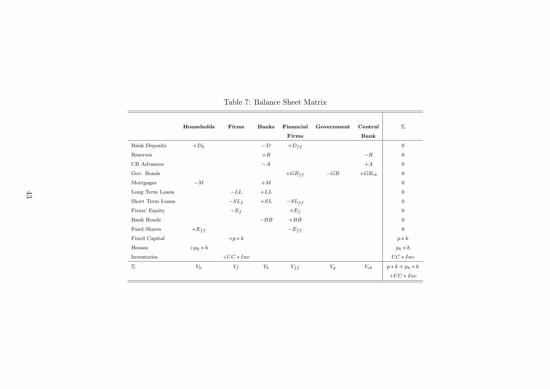
Table 7: Balance Sheet Matrix

Households Firms Banks Financial Government Central Σ

Firms Bank

Bank Deposits +Dh −D +Dff 0

Reserves +R −R 0

CB Advances −A +A 0

Gov. Bonds +GBff −GB +GBcb 0

Mortgages −M +M 0

Long Term Loans −LL +LL 0

Short Term Loans −SLf +SL −SLff 0

Firms’ Equity −Ef +Ef 0

Bank Bonds −BB +BB 0

Fund Shares +Eff −Eff 0

Fixed Capital +p ∗ k p ∗ k

Houses +ph ∗ h ph ∗ h

Inventories +UC ∗ Inv UC ∗ Inv

Σ Vh Vf Vb Vff Vg Vcb p ∗ k + ph ∗ h

+UC ∗ Inv

43

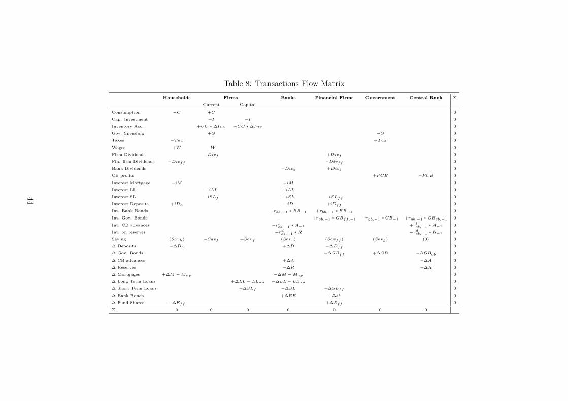
Table 8: Transactions Flow Matrix

Households Firms Banks Financial Firms Government Central Bank Σ

Current Capital

Consumption −C +C 0

Cap. Investment +I −I 0

Inventory Acc. +UC ∗ ∆Inv −UC ∗ ∆Inv 0

Gov. Spending +G −G 0

Taxes −Tax +Tax 0

Wages +W −W 0

Firm Dividends −Divf +Divf 0

Fin. firm Dividends +Divff −Divff 0

Bank Dividends −Divb +Divb 0

CB profits +PCB −PCB 0

Interest Mortgage −iM +iM 0

Interest LL −iLL +iLL 0

Interest SL −iSLf +iSL −iSLff 0

Interest Deposits +iDh −iD +iDff 0

Int. Bank Bonds −rbb,−1 ∗ BB−1 +rbb,−1 ∗ BB−1 0

Int. Gov. Bonds +rgb,−1 ∗ GBff,−1 −rgb,−1 ∗ GB−1 +rgb,−1 ∗ GBcb,−1 0

Int. CB advances −rlcb,−1 ∗ A−1 +rlcb,−1 ∗ A−1 0

Int. on reserves +rdcb,−1 ∗ R −rdcb,−1 ∗ R−1 0

Saving (Savh) −Savf +Savf (Savb) (Savff ) (Savg) (0) 0

∆ Deposits −∆Dh +∆D −∆Dff 0

∆ Gov. Bonds −∆GBff +∆GB −∆GBcb 0

∆ CB advances +∆A −∆A 0

∆ Reserves −∆R +∆R 0

∆ Mortgages +∆M − Mnp −∆M − Mnp 0

∆ Long Term Loans +∆LL − LLnp −∆LL − LLnp 0

∆ Short Term Loans +∆SLf −∆SL +∆SLff 0

∆ Bank Bonds +∆BB −∆bb 0

∆ Fund Shares −∆Eff +∆Eff 0

Σ 0 0 0 0 0 0 0

44