Embed Size (px)
Citation preview
UPTEC X 06 038 ISSN 1401-2138 AUG 2006 PÄR BJELKMAR
Molecular dynamics simulations; comparisons of octameric and tetrameric channel models of the peptaibol antiamoebin Master’s degree project
Molecular Biotechnology Programme Uppsala University School of Engineering
UPTEC X 06 038 Date of issue 2006-08 Author
Pär Bjelkmar Title (English)
Molecular dynamics simulations; comparisons of octameric and tetrameric channel models of the peptaibol antiamoebin
Title (Swedish) Abstract Two different models of the channel bundle of the peptaibol antiamoebin were studied using molecular dynamics simulations in an explicitly modeled environment consisting of a POPC bilayer surrounded by water. Both the octameric and tetrameric bundles were found to be stable over tenths of nanoseconds with characteristic interhelical hydrogen bonding patterns stabilizing the channels. The dimensions of the channels have also been assessed and compared to each other and the modern potassium channels.
Keywords antiamoebin, molecular dynamics, channel modeling, ion channels, protobiotic evolution
Supervisors Andrew Pohorille
NASA Ames Research Center, California USA Scientific reviewer
Johan Åqvist Department of Cell & Molecular Biology, Uppsala University
Project name
Sponsors
Language English
Security Secret until 2007-09-01
ISSN 1401-2138
Classification
Supplementary bibliographical information Pages 33
Biology Education Centre Biomedical Center Husargatan 3 Uppsala Box 592 S-75124 Uppsala Tel +46 (0)18 4710000 Fax +46 (0)18 555217
Molecular dynamics simulations; comparisons of octameric and tetrameric channel models of the
peptaibol antiamoebin
Pär Bjelkmar
Sammanfattning Forskargruppen som jag arbetade för på NASA studerar olika processer viktiga för uppkomsten av liv. En av tyngdpunkterna är att undersöka och försöka förklara hur de första membranproteinerna uppstod och utvecklades till de avancerade molekylära maskiner de är idag. Membranproteiner är essentiella för cellulärt liv eftersom ett cellmembran endast är permeabelt för ett fåtal, små, molekyltyper. För att transportera andra nödvändiga ämnen över membranet så måste cellerna aktivt öppna passager. Detta är en av huvudfunktionerna för membranproteiner. Antiamoebin är en molekyl som utsöndras av vissa svampar i försvar mot parasiter samt som ett vapen för att freda sin livsmiljö mot konkurrerande organismer. Det är en kort peptid formad som en korkskruv. Flertalet sådana associerar och bildar kanaler i cellmembranet hos målorganismen. Då startar ett för cellen okontrollerat flöde av molekyler över membranet och därmed oskadliggörs cellen. Jag har i detta projekt studerat dessa antiamoebin-kanaler med hjälp av datorsimuleringar för att försöka förstå hur den funktionella formen av kanalen ser ut och fungerar. Detta är intressant ur ett ”uppkomsten-av-liv”– perspektiv eftersom de individuella byggklotsarna är relativt korta, de syntetiseras utan inblandning av genomet, och kanalen har analoga strukturella element med moderna jonkanaler.
Examensarbete 20p Civilingenjörsprogrammet i Bioinformatik
Uppsala universitet, augusti 2006
Table of contents TABLE OF CONTENTS 1
CHAPTER 1: INTRODUCTION 2
1.1 STRUCTURE OF TEXT 2 1.2 BACKGROUND AND MOTIVATION 2 1.3 AIMS 5 1.4 MOLECULAR MODELING 5 1.4.1 OVERVIEW 6 1.4.2 DEFINING EMPIRICAL FORCE FIELDS 8 1.5 OVERVIEW OF SOFTWARE 10 1.5.1 NAMD 11 1.5.2 VMD 11 1.6 PARALLEL COMPUTING ON NAS COLUMBIA 12
CHAPTER 2: METHODOLOGY 12
2.1 PARAMETERIZATION: BUILDING NON-STANDARD RESIDUES 12 2.2 CONSTRUCTION OF ANTIAMOEBIN MONOMER 13 2.3 GENERAL SIMULATION PARAMETERS 13 2.4 VALIDATION OF MONOMER MODEL 14 2.4.1 AAM IN HEXANE 15 2.4.2 AAM IN METHANOL 15 2.4.3 AAM IN POPC LIPID BILAYER 16 2.5 CONSTRUCTION OF TRANSMEMBRANE CHANNEL 16 2.5.1 OCTAMERIC BUNDLE 17 2.5.2 TETRAMERIC BUNDLE 18
CHAPTER 3: RESULTS 19
3.1 MONOMER VALIDATION 19 3.1.1 AAM IN HEXANE 19 3.1.2 AAM IN METHANOL 20 3.1.3 AAM IN POPC MEMBRANE 20 3.2 OCTAMERIC MODEL 22 3.3 TETRAMERIC MODEL 23
CHAPTER 4: DISCUSSION 26
4.1 AAM MONOMER 26 4.2 OCTAMERIC CHANNEL MODEL 28 4.3 TETRAMERIC CHANNEL MODEL 29
ACKNOWLEDGMENTS 31
REFERENCES 32
Pär Bjelkmar, Aug 2006
2
Chapter 1: Introduction This report is the presentation of the work performed in my degree project for the Bioinformatics engineering program at Uppsala University. The project duration is 20 weeks and it was conducted March-July 2006 at NASA Ames Research Center in California, USA under supervision of Dr. Andrew Pohorille.
1.1 Structure of text This work is divided into four chapters. In the first, a general introduction of the concepts is given, both the theoretical fundamentals of molecular modeling and what is known about the specific molecule studied. The software and hardware used is presented, and of course, the motivation for why this particular molecule is studied and which questions the work aims to help answering is specified. A detailed description of the methodology used and the acquired results follows in chapters 2 and 3. In chapter 4, the work is sewn together, hopefully giving it a less fragmented appearance. The conclusions are also gathered and discussed in this chapter. The report finishes of with Acknowledgments and References. Concerning where to put the theory underlying this work, I decided having a general discussion of the foundations of molecular modeling in chapter 1 of this document whereas the more specific techniques used in the project are presented to the reader in chapter 2 as they were encountered during the course of the work. In this manner the pivot elements of the project are distinct from the part necessary for the completeness and the introduction to readers new to the field (or in need of some refreshening of the concepts).
1.2 Background and motivation Antiamoebin (AAM) is a small ensemble of peptides originally isolated the fungal Emericel-lopsis family [1], but has also been shown to be produced by other groups of fungi, e.g. the Stilbellas [2]. The major component is AAM I, from now on referred to AAM without enu-meration, having the amino acid sequence:
Ac-Phe-Aib-Aib-Aib-Iva-Gly-Leu-Aib-Aib-Hyp-Gln-Iva-Hyp-Aib-Pro-Phol
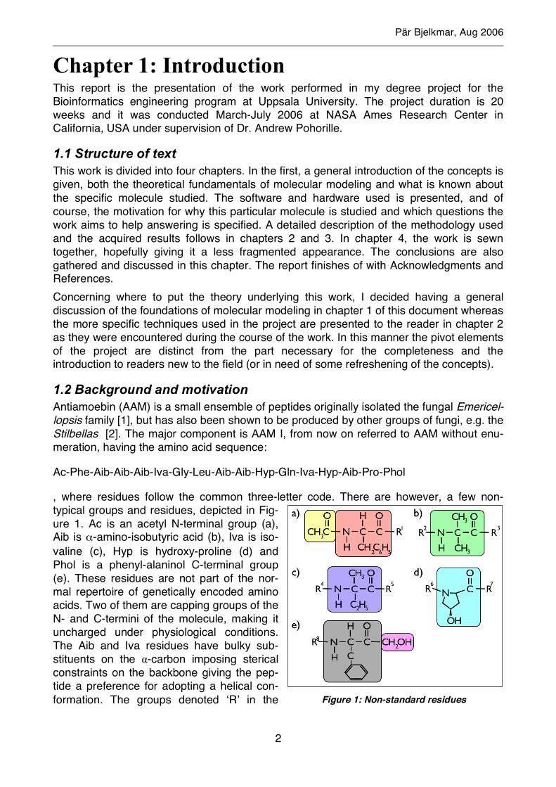
, where residues follow the common three-letter code. There are however, a few non-typical groups and residues, depicted in Fig-ure 1. Ac is an acetyl N-terminal group (a), Aib is α-amino-isobutyric acid (b), Iva is iso-valine (c), Hyp is hydroxy-proline (d) and Phol is a phenyl-alaninol C-terminal group (e). These residues are not part of the nor-mal repertoire of genetically encoded amino acids. Two of them are capping groups of the N- and C-termini of the molecule, making it uncharged under physiological conditions. The Aib and Iva residues have bulky sub-stituents on the α-carbon imposing sterical constraints on the backbone giving the pep-tide a preference for adopting a helical con-formation. The groups denoted ‘R’ in the Figure 1: Non-standard residues
Pär Bjelkmar, Aug 2006
3
figure are symbols of the remaining, not visualized, part(s) of the molecule.
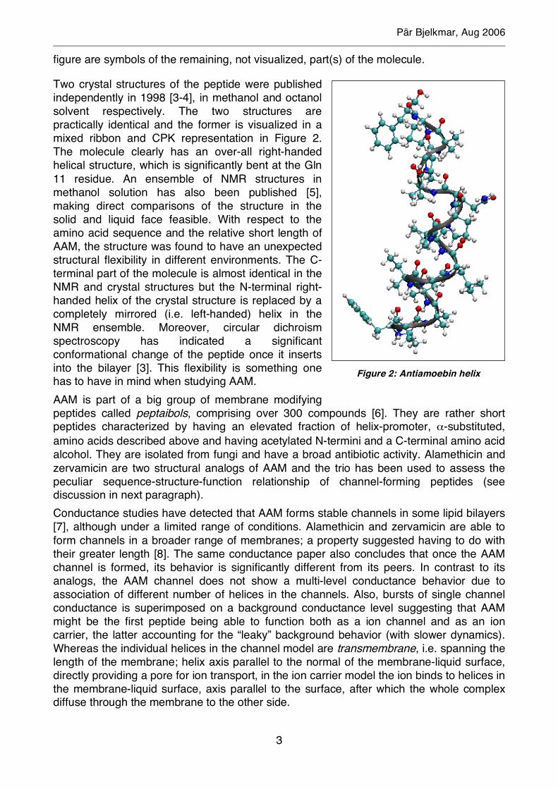
Two crystal structures of the peptide were published independently in 1998 [3-4], in methanol and octanol solvent respectively. The two structures are practically identical and the former is visualized in a mixed ribbon and CPK representation in Figure 2. The molecule clearly has an over-all right-handed helical structure, which is significantly bent at the Gln 11 residue. An ensemble of NMR structures in methanol solution has also been published [5], making direct comparisons of the structure in the solid and liquid face feasible. With respect to the amino acid sequence and the relative short length of AAM, the structure was found to have an unexpected structural flexibility in different environments. The C-terminal part of the molecule is almost identical in the NMR and crystal structures but the N-terminal right-handed helix of the crystal structure is replaced by a completely mirrored (i.e. left-handed) helix in the NMR ensemble. Moreover, circular dichroism spectroscopy has indicated a significant conformational change of the peptide once it inserts into the bilayer [3]. This flexibility is something one has to have in mind when studying AAM. AAM is part of a big group of membrane modifying peptides called peptaibols, comprising over 300 compounds [6]. They are rather short peptides characterized by having an elevated fraction of helix-promoter, α-substituted, amino acids described above and having acetylated N-termini and a C-terminal amino acid alcohol. They are isolated from fungi and have a broad antibiotic activity. Alamethicin and zervamicin are two structural analogs of AAM and the trio has been used to assess the peculiar sequence-structure-function relationship of channel-forming peptides (see discussion in next paragraph). Conductance studies have detected that AAM forms stable channels in some lipid bilayers [7], although under a limited range of conditions. Alamethicin and zervamicin are able to form channels in a broader range of membranes; a property suggested having to do with their greater length [8]. The same conductance paper also concludes that once the AAM channel is formed, its behavior is significantly different from its peers. In contrast to its analogs, the AAM channel does not show a multi-level conductance behavior due to association of different number of helices in the channels. Also, bursts of single channel conductance is superimposed on a background conductance level suggesting that AAM might be the first peptide being able to function both as a ion channel and as an ion carrier, the latter accounting for the “leaky” background behavior (with slower dynamics). Whereas the individual helices in the channel model are transmembrane, i.e. spanning the length of the membrane; helix axis parallel to the normal of the membrane-liquid surface, directly providing a pore for ion transport, in the ion carrier model the ion binds to helices in the membrane-liquid surface, axis parallel to the surface, after which the whole complex diffuse through the membrane to the other side.
Figure 2: Antiamoebin helix
Pär Bjelkmar, Aug 2006
4
The functional duality gives the first indication that AAM could be an interesting peptide to study in a protobiological point of view; how the origin and evolution of membrane proteins took place in the early beginning of life, in the so called protocells. Since the carrier mechanism most certainly would account for the more ancient mechanism of the pair (simply because it is the less optimized process, involving less complexity; Occam’s rule) one might think of AAM as being a molecule on the verge of adopting a new, more advanced function. Having said this it does not necessarily imply that the channel function is selected for in AAM, only that since the peptide appear to be able to function in either way, it could be used to investigate the molecular causes of this functional flexibility and provide a model for how the first transmembrane channels could have evolved. AAM has antibiotical properties and is secreted by the fungi as a general microbial defense [9] and as a mean for defending its habitat in highly competitive environments [2]. It has been shown to be an uncoupler of the oxidative phosphorylation [10] as well as having antimalaria activity [11]. In both cases the peptide inserts into the target cells’ membranes and once in place, dissipating the membrane potential by transporting ions over the membranes. Although the detailed structure of the AAM channel is not known, in 2003 a theoretical model was presented based on the conductance studies and structural information from the crystal and NMR structures [12]. This structure has interesting features in that it presents an overall negatively charged electrostatic lumen, promoting formation of cation interactions. It made the authors to structurally compare features of this model with naturally occurring potassium channels with known structure, named KcsA and MethK. They are well-studied channels; also cation transporters (but with a high selectivity for potassium ions) and does not show signs of multi-level conductance. However, they have a much more complex structure compared to the rather primitive AAM channel, which is considerably smaller and have constituents not encoded by the genome. Despite the apparent difference in complexity, the AAM model channel shows considerable structural similarities the authors argue. This is a very important paper, laying the foundation for this project and I will come back to it many times in this report, in particular in chapter 4. The observation discussed in the previous paragraph has implications considering the origin and evolution of membrane proteins and is the main cause for me to study it. If the relatively simple AAM channel is able to perform functions associated with significantly more advanced channels (or modern if you’d like), it could be used as a model for an ancestral state of the potassium channel. After all, in the Darwinian model of evolution, nothing has evolved in an instant: it is a gradual process of tiny changes driven by natural selection, ever increasing the fitness of the entity in the contemporary environment. This holds for both macroscopical entities such as animals as well as on the microscopic level of the protein molecules within them. An immediate consequence is that there must be ancestral states of the modern ion channels and the reasoning above suggests AAM could be used as a model for such a one. However, the similarities of the channels are structural and the detailed mechanism of action of the AAM channel is not known. Thus, to assess the functional relationship of the channels one have to study the dynamics of ion transport in the AAM channel [13]. Another interesting property of the AAM molecule in origin of life research is the presence of atypical amino acids not coded for by the genome. In fact the AAM peptide has no gene at all, in stead the peptide is most certain synthesized in non-ribosomal pathways by specific enzymatic complexes [14]. In early environments on earth, these amino acids were possibly as abundant as the standard ones and could be incorporated in simple
Pär Bjelkmar, Aug 2006
5
peptides. In the light of the fact that such peptides could be biologically active they give credence to the model of non-genomic origin of life. At some later point the genome emerged, and during the course of time these residues have been selected against for some reason, ultimately excluding them from the pool of genetically coded residues.
1.3 Aims Now, when the motivation for studying the AAM molecule and the channel it forms has been given it is time to specify more concrete aims of this project. Taking the available time into account and adding some naive optimism, I had intended to be able to treat the following points of interest.
• Extend the current CHARMM force field with the non-standard residues in AAM. • Construct a model and perform molecular dynamics simulations of the AAM
monomer. • Construct a model and perform MD simulations of the AAM channel inserted into a
membrane bilayer. • Study the structural properties of the channel when it has been “equilibrated”, in
particular: - Which interactions hold the channel together? - What does the channel pore look like? - Are there structural similarities to more complex ion channels?
• Study ion-channel interactions: - Does the AAM channel reduce the energy required to transport ions over the
membrane, difference between cations and anions? - Calculate free-energy profiles of the ion transport through the channel. - Compare the mechanism of ion transport with the more complex ion
channels.
1.4 Molecular modeling We now turn to the underlying principles of molecular modeling and the usual confusion regarding terminology. Molecular modeling is a general term including all methods dealing with building models of molecules. Another analogous term used is computational chemistry. The models have several uses, for example: visualization, structural and dynamical investigation and for prediction and calculation of various, often measurable properties such as energies, temperature, volume, pressure, etc. Normally, I would say, molecular modeling is thought to be something closely associated with being performed by computers, but before computational dawn, scientist built (and still do for some applications, mostly educational) non-virtual models of molecules, typically on a piece of paper or with other available stationary as pencils and rubbers. Also more detailed physical models such as the office-sized, famous Watson and Crick model of the DNA helix have been constructed. Calculation and prediction of properties of the studied molecules in those times were practical only for very small and idealized systems. Computers revolutionized the field of (molecular) modeling, and tedious calculations could be performed by computers and hence bigger and bigger systems could be considered, and in more detail. Nowadays, the field of molecular modeling is widespread and a very important tool in various applications and there are numerous books written on the subject,
Pär Bjelkmar, Aug 2006
6
see for example [15-16]. It is impossible to incorporate a somewhat detailed description of the field in a report such as this. However, besides turning to, for this project relevant parts of the field, I will try to give a very short overview of the related methodologies to put the techniques used here in a bigger perspective.
1.4.1 Overview The most apparent division of molecular simulations is the distinction of methods where electrons are explicitly modeled, often called quantum mechanics or quantum chemistry, e.g. ab initio methods, and where they are not, named empirical force field methods, e.g. molecular dynamics (MD) and Monte Carlo simulations (MC). I start with briefly discussing the former part of models, the quantum mechanical ones. The majority of computational chemistry methods build on the Born-Oppenheimer approximation. The higher velocities of the electrons relative to the nuclei allow us to consider the two motions as uncoupled; as the coordinates of a nucleus change the much faster timescale of the electrons surrounding it let them instantaneously adjust to the new position of the nuclei. Consequently a less complicated form of the Schrödinger equation can be used in the quantum mechanical methods and it also justifies the approach of molecular mechanics (next section). Still, note the difference that electrons in fact are explicitly modeled in quantum mechanical models, in contrast to empirical force field models where only the positions of the nuclei are considered. Therefore, the quantum mechanics approach allows studying processes where permanent changes of electronic densities are important, as in chemical reactions where bonds are created and broken. Methods developed solely on theoretical results, i.e. where the integrals of a given approximation are explicitly solved, are called ab initio whereas models, which incorporate experimental results to solve these integrals, are called semi-empirical. In some semi-empirical models all electrons are not considered, but they still comprise significantly more bodies than the empirical force field models. The underlying equation of quantum mechanical models is the Schrödinger equation, where sets of certain carefully characterized mathematical functions are used to describe the molecular system. From those the energies of the molecule can be calculated. The equation is only possible to solve analytically in a hand-full of very small systems with no practical interest. For larger systems more and more approximations have to be incorporated and the equations have to be solved numerically on a computer. Even though both computer technology has evolved enormously in recent decades and efficient algorithms for numerical methods have been developed, these methods are still very computationally expensive. To study typically large systems of biomolecules using them are quite impractical, if not impossible, today. Fortunately, there are other methods available to cope with these problems to which we now turn.
1.4.1.1 Empirical force field methods Empirical force field methods, or molecular mechanics (MM), are based on describing the interactions between atoms by classical mechanics. In stead of treating every atom quantum mechanically, they are modeled as points in space associated with a permanent charge, i.e. the electrons together with the nucleus of a certain atom are collectively assigned one single charge value which in each case is dependent on the surrounding chemical environment. The result is that all atoms can be described as point charges and hence well-known classical expressions for interactions between such can be used. For now (construction of such force fields will be described in the section 1.4.2) it is enough to
Pär Bjelkmar, Aug 2006
7
say that these force fields are expressions involving huge numbers of parameters associated with different interactions between different atom types. To assign values to these parameters is called parameterization and is a field of its own. Transferability is a key property of such parameters; those deduced from experiments on small systems could be used for corresponding parts in a much larger system, as in a biopolymer for example. The transferability is something I used in the parameterization of the atypical amino acids present in the antiamoebin molecule (see section 2.1).
1.4.1.2 Minimization Assume now that a force field of a system has been constructed. One is consequently able to start exploring its properties. One interesting thing to study is the so-called potential en-ergy surface. It is a multidimensional surface describing the potential energy landscape of the system as a function of the coordinates of the atoms. For a system with N atoms this hypersurface in principle has 3N dimensions (3N-6 for a non-symmetrical system). Every change of the coordinates of one or several atoms normally results in an alteration of the (potential) energy. By studying the surface it is for example possible to assess the most stable conformations of the system at hand. These stable points are the stationary points of the surface where the first derivative of the energy is zero with respect to the atomic co-ordinates. If the stationary point is a minimum it is called a local minimum. The local mini-mum with the lowest energy is called the global minimum and is the most stable state of the system. Identifying such stable conformations in the context of molecular modeling is simply called minimization, or structural minimization. Minimization of functions is a stan-dard problem in mathematics and is thus a well-studied subject and since it only plays a minor role in this project I leave it to the interested to read about it elsewhere.
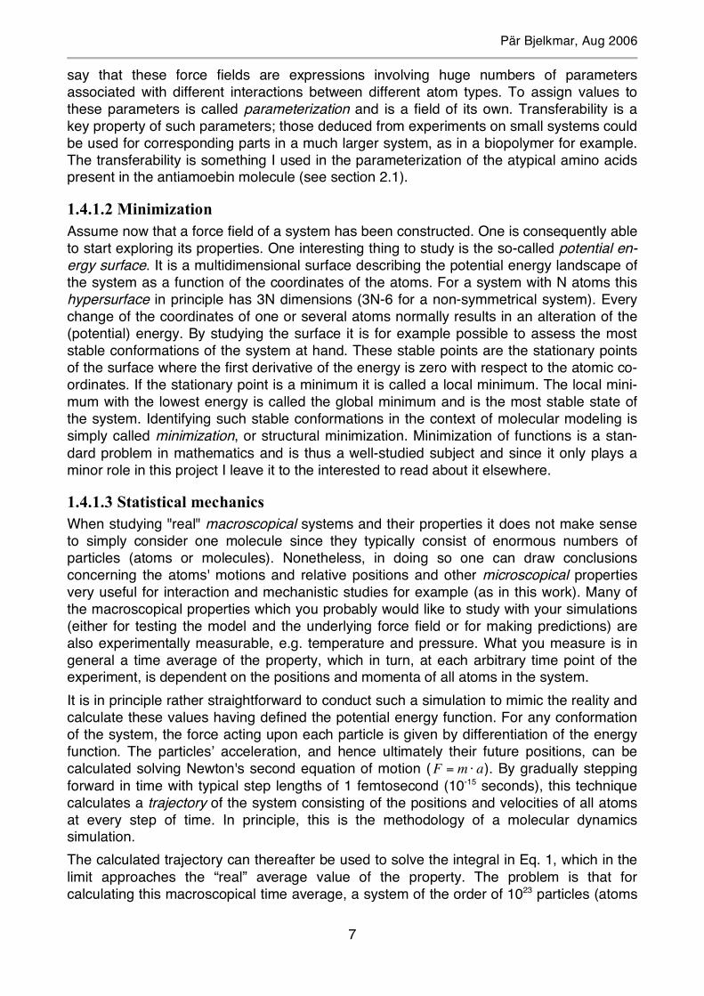
1.4.1.3 Statistical mechanics When studying "real" macroscopical systems and their properties it does not make sense to simply consider one molecule since they typically consist of enormous numbers of particles (atoms or molecules). Nonetheless, in doing so one can draw conclusions concerning the atoms' motions and relative positions and other microscopical properties very useful for interaction and mechanistic studies for example (as in this work). Many of the macroscopical properties which you probably would like to study with your simulations (either for testing the model and the underlying force field or for making predictions) are also experimentally measurable, e.g. temperature and pressure. What you measure is in general a time average of the property, which in turn, at each arbitrary time point of the experiment, is dependent on the positions and momenta of all atoms in the system. It is in principle rather straightforward to conduct such a simulation to mimic the reality and calculate these values having defined the potential energy function. For any conformation of the system, the force acting upon each particle is given by differentiation of the energy function. The particles’ acceleration, and hence ultimately their future positions, can be calculated solving Newton's second equation of motion (
!
F = m " a). By gradually stepping forward in time with typical step lengths of 1 femtosecond (10-15 seconds), this technique calculates a trajectory of the system consisting of the positions and velocities of all atoms at every step of time. In principle, this is the methodology of a molecular dynamics simulation. The calculated trajectory can thereafter be used to solve the integral in Eq. 1, which in the limit approaches the “real” average value of the property. The problem is that for calculating this macroscopical time average, a system of the order of 1023 particles (atoms
Pär Bjelkmar, Aug 2006
8
or molecules), all moving and interacting through time, have to be considered; a task that is currently far from possible to solve. In pursuing to bridge this gap between the microscopical and macroscopical worlds, Boltzmann and his contemporaries developed the theory of statistical mechanics. In statistical mechanics this time average is replaced, according to the ergodic hypothesis (one of the postulates of statistical mechanics), by the ensemble average, which consists of a large number of configurations of the system generated by the simulation.
!
< A >= lim"#$
1
"A(p
N(t),r
N(t))dt =
e.h.
t= 0
"
% A(pN,r
N) & p(pN ,rN )dpNdrN%% Eq. 1
The notation ‘< >‘ indicate the average of an arbitrary thermodynamic property A and the double integral is a practical way to denote the actual 6N integrals (one for each coordinate of the N particles and one for the momentum in each direction). The notation
!
p(pN,r
N) is the probability density function for finding the system with momenta
!
pN and positions
!
rN . Under conditions of constant number of particles, constant volume
and constant temperature (NVT ensemble or the canonical ensemble), the probability density function is the famous Boltzmann distribution.
!
p(pN,r
N) = e
"E (p
N,rN)
kBT /Q Eq. 2 The exponent
!
E(pN,r
N) is the energy,
!
kB is the Boltzmann constant and
!
Q is the (molecular) partition function, in turn essentially an expression of standard results obtained by solving the Schrödinger equation. In such a way, statistical mechanics provide us with the awestruck tool to tie together modern quantum mechanics with thermodynamics developed already during the seventeenth century, giving us a hands-on proof of the validity and power of quantum mechanics. The two computational simulation techniques, MD and MC, generate (or sample as one often say) structures from the Boltzmann distribution. Briefly, the difference is that MC performs a random walk through conformational space and accepts new conformations in a particular way so the acquired sates are sampled from the Boltzmann distribution. The random nature of the sampling has the consequence that consecutive states have no real connection in time. MD on the other hand, generates a trajectory of states reflecting the true dynamics of the system. When an ensemble of states have been generated (typically after several hundred or thousand picoseconds of simulation) a time average of the property is calculated by numerical integration of the right hand part of Eq. 1:
!
< A >=1
MA(pi
N,ri
N)
i=1
M
" Eq. 3
, where
!
M is the number of time steps of the simulation.
1.4.2 Defining empirical force fields Molecular mechanics, or empirical force field methods, are techniques used to sidestep the computationally expensive quantum mechanical methods. Even though one might get the impression that QM is superior to MM, the latter class of methods is in many cases as accurate as the most detailed QM calculation and they are finished in a fraction of the time.
Pär Bjelkmar, Aug 2006
9
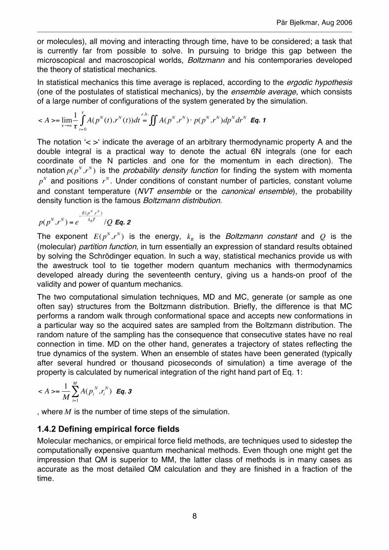
An empirical force field is in general an expression relating the total potential energy of the system to the coordinates of the atoms. In this sense the name is somewhat misleading because it is an expression of the energy, not the force. However, since differentiation of the energy function gives the force, the choice of name is quite arbitrary. Different contributions to the potential energy is modeled as mathematical functions and their parameters are derived from various types of experiments, hence the word ‘empirical’ in the name. There are many force fields out there; the underlying idea behind them all is generally quite similar but there are several ways to come up with an acceptable one and the mathematical functions used to describe the different contributions to the potential energy is numerous and chosen quite ad hoc. Force fields are often developed specifically for a certain group of molecules and sometimes also for a certain application. The CHARMM force field (www.charmm.org) was used in this work and I will discuss it more in detail below. Note that although I in particular only treat one force field, the basic principle is, as I said, rather general. An example of the CHARMM force field expression for the potential energy looks like:
V (r)=
!
K" (" #"0)2
+ K$ ($ #$0)2
+ K% (1+ cos(n(%) #&)) + K' (' +'0)2
impropers
(dihedrals
(angles
(bonds
( +
!
+ 4"ij# ij
rij
$
% & &
'
( ) )
*
+ , ,
$
%
& &
nonbondedpairs i, j
-12
.# ij
rij
$
% & &
'
( ) )
6/
0
1 1 + k
qiq j
rij
'
( ) ) Eq. 4
The first four terms are due to bonded interactions; interactions emerging from the structural restrains atoms infer on each other because they are stuck together in a molecule, and the last two are non-bonded interactions; which are interactions mediated “through space” such as the electrostatic interaction between two charges. In Figure 3, the different contributions to the potential energy are schematically illustrated. Whereas the bonded interactions are interactions between atoms within a continuous sequence of length four in a molecule (1-2-3-4 interactions) the bonded interactions are in principle necessary to calculate between all pairs of atoms in the system. The non-bonded terms are consequently critical for the computational cost of the calculation of the energy and much effort has been put into the development of efficient methods for their treatment. Term one, with ‘bonds’ subscript, represents the energetic penalty for the stretching and compression of diatomic bonds (a). It is described as a harmonic potential and the energy is proportional (with proportionality constant
!
K" ) to the square of the displacement from the reference bond length,
!
"0. As in all these
terms, the parameters are in general dependent on the atom types involved in the bond. Atom type when used within empirical force fields often has a broader meaning than simply the element type, it is also used for different hybridization states, e.g. sp3 and sp2 carbon, and
Figure 3: Energy contributions
Pär Bjelkmar, Aug 2006
10
other properties for certain chemical groups. The very simple, but still often sufficient, quadratic functional form of the diatomic bond has many alternatives, as the well-known Morse potential for example. Around the reference bond length the harmonic potential is in good agreement with the Morse potential and experience shows that the tradeoff between using a Morse potential, requiring three parameters for each bond and more operations to compute, and the simple quadratic potential favors the latter (at least in applications such as this project). The second term describes the behavior of the energy when the angle between three atoms is altered (b). As in the bond term they are modeled by a harmonic function, with parameters denoted
!
K" and
!
"0. This functional form is also used for the improper term of
the energy function (d), which is aiming to account for the planarity of certain molecular groups (as the peptide bond for example). In this case the parameters are named
!
K" and
!
"0.
Last of the bonded interactions is the dihedral term which also sometimes is called the torsional term (c). Four consecutive atoms in the molecule define it and it is caused by the energy alteration of rotating the first and fourth atom around the bond between the second and third atom. It is not surprising that a periodic function of the angle
!
" is used here.
!
K" models the amplitude,
!
n the multiplicity and
!
" the phase shift of the energy extremes. Non-bonded interactions are divided into two types; electrostatic interactions (f), described by Coulomb’s law and van der Waal interactions (e), due to the repulsion of atoms (in fact it is the electrons of the two atoms that repel each other) at very small separations and their attraction, caused by induced temporal dipoles, at longer. They are both functions of inverse powers of the distance between atom pairs and ideally their contributions to the energy have to be calculated for all pairs of molecules in the system. However, this is in practice never done because of the immense number of such pairs in big systems, proportional to N2 (in my case N ~105 atoms). Instead one uses cutoffs; atom pairs separated by a distance greater than a certain user-defined distance are simply neglected. The accuracy of the simulation is especially sensitive to how the electrostatic interactions are treated since they decrease as 1/r compared to the much more radically decreasing terms in the van der Waal expression (1/r6 and 1/r12). For these Coulomb interactions, the cutoff approach is insufficient for many systems and identifying this problem, scientists developed a method for full electrostatic interaction calculations where the computational cost scales as
!
N " log(N) [17]. The method is called Particle Mesh Ewald (PME) and is now a standard method used within molecular simulations. These technical details (including many more) of how to actually use the information in the force field are not formally part of the force field but are instead treated in the molecular simulation software used. A bisectional structure of a CHARMM force field separate the connectivity (i.e. how the molecules are bonded together), charge and mass information of atoms into a topology file and the specific parameters for all different atom types for all different functional terms into a parameter file (more on these below).
1.5 Overview of software The molecular simulation and visualization software used during the project are the NAMD and VMD programs from the Theoretical Biophysics Group at University of Illinois and Beckham Institute, freely available from www.ks.uiuc.edu/Research/. The programs run on most Unix systems, Windows and MacOS X. NAMD [18] is a molecular dynamics package implemented to be able to utilize the often-needed computational power of multiple
Pär Bjelkmar, Aug 2006
11
processors, running the calculations in parallel. Its sister program VMD performs analysis and visualization of molecules and calculated trajectories.
1.5.1 NAMD The NAMD package calculates the trajectory of the system of interest by numerically solving the equations of motion for all atoms. It calculates both bonded 1-2-3-4 interactions and non-bonded interactions between pair of atoms using an empirical force field, such as the CHARMM force field discussed in 1.4.2. A brief description of MD is provided in 1.4.1. The software also has the capability of minimization of molecular structures. To set-up a simulation in NAMD there are a few things needed:
• A PSF file defining the molecular structure of the system. • A PDB file containing the coordinates of all atoms. • Force field parameter file(s) in CHARMM, X-PLOR, GROMACS or AMBER formats. • A configuration file specifying the simulation options to be used in the simulation.
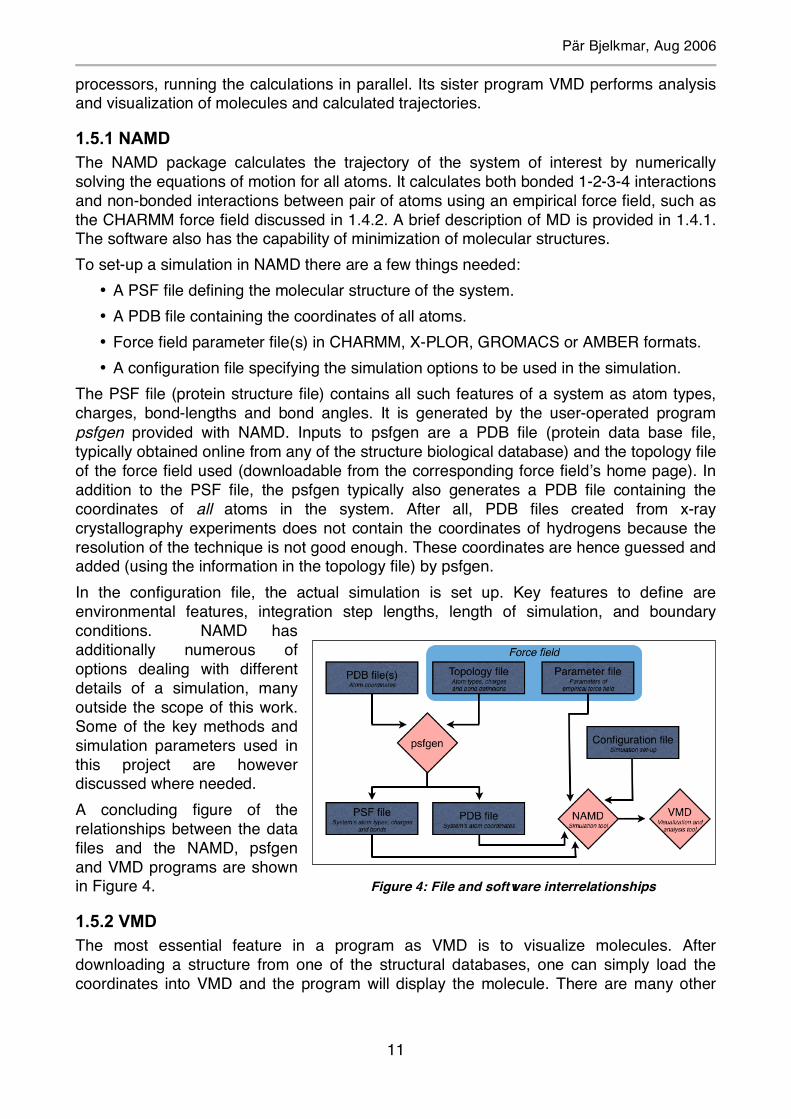
The PSF file (protein structure file) contains all such features of a system as atom types, charges, bond-lengths and bond angles. It is generated by the user-operated program psfgen provided with NAMD. Inputs to psfgen are a PDB file (protein data base file, typically obtained online from any of the structure biological database) and the topology file of the force field used (downloadable from the corresponding force field’s home page). In addition to the PSF file, the psfgen typically also generates a PDB file containing the coordinates of all atoms in the system. After all, PDB files created from x-ray crystallography experiments does not contain the coordinates of hydrogens because the resolution of the technique is not good enough. These coordinates are hence guessed and added (using the information in the topology file) by psfgen. In the configuration file, the actual simulation is set up. Key features to define are environmental features, integration step lengths, length of simulation, and boundary conditions. NAMD has additionally numerous of options dealing with different details of a simulation, many outside the scope of this work. Some of the key methods and simulation parameters used in this project are however discussed where needed. A concluding figure of the relationships between the data files and the NAMD, psfgen and VMD programs are shown in Figure 4.
1.5.2 VMD The most essential feature in a program as VMD is to visualize molecules. After downloading a structure from one of the structural databases, one can simply load the coordinates into VMD and the program will display the molecule. There are many other
Figure 4: File and software interrelationships
Pär Bjelkmar, Aug 2006
12
free packages for molecular visualization and analysis, the most known is probably RasMol (www.openrasmol.org). VMD was constructed to be used in parallel to the NAMD molecular simulation package. It easily loads computed trajectories from NAMD and besides an extensive menu of graphical options, enabling the user to represent arbitrary parts of the molecule in different visualization types, the program also provides several integrated and powerful analysis and model modification tools. The ones I have been using most frequently in this work are the tools to plot (predicted) secondary structure of a peptide over time and for creation of membrane bilayers. On top of these, there is a Tcl (www.tcl.tk) text command interface making it easy to write your own programs for interaction with the calculations. In this way, scripts like the ones imposing restraints on ions and for computing the root mean square deviations (RMSD) were created.
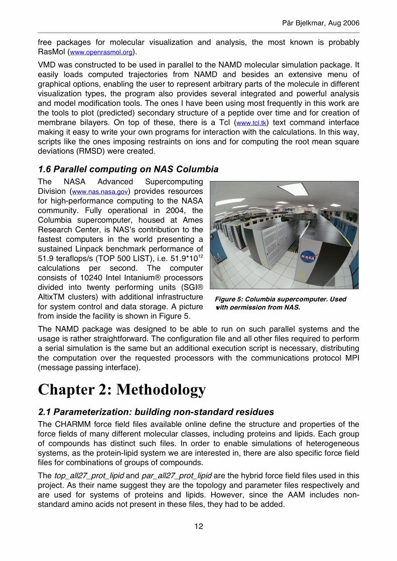
1.6 Parallel computing on NAS Columbia The NASA Advanced Supercomputing Division (www.nas.nasa.gov) provides resources for high-performance computing to the NASA community. Fully operational in 2004, the Columbia supercomputer, housed at Ames Research Center, is NAS’s contribution to the fastest computers in the world presenting a sustained Linpack benchmark performance of 51.9 teraflops/s (TOP 500 LIST), i.e. 51.9*1012 calculations per second. The computer consists of 10240 Intel Intanium® processors divided into twenty performing units (SGI® AltixTM clusters) with additional infrastructure for system control and data storage. A picture from inside the facility is shown in Figure 5. The NAMD package was designed to be able to run on such parallel systems and the usage is rather straightforward. The configuration file and all other files required to perform a serial simulation is the same but an additional execution script is necessary, distributing the computation over the requested processors with the communications protocol MPI (message passing interface).
Chapter 2: Methodology 2.1 Parameterization: building non-standard residues The CHARMM force field files available online define the structure and properties of the force fields of many different molecular classes, including proteins and lipids. Each group of compounds has distinct such files. In order to enable simulations of heterogeneous systems, as the protein-lipid system we are interested in, there are also specific force field files for combinations of groups of compounds. The top_all27_prot_lipid and par_all27_prot_lipid are the hybrid force field files used in this project. As their name suggest they are the topology and parameter files respectively and are used for systems of proteins and lipids. However, since the AAM includes non-standard amino acids not present in these files, they had to be added.
Figure 5: Columbia supercomputer. Used with permission from NAS.
Pär Bjelkmar, Aug 2006
13
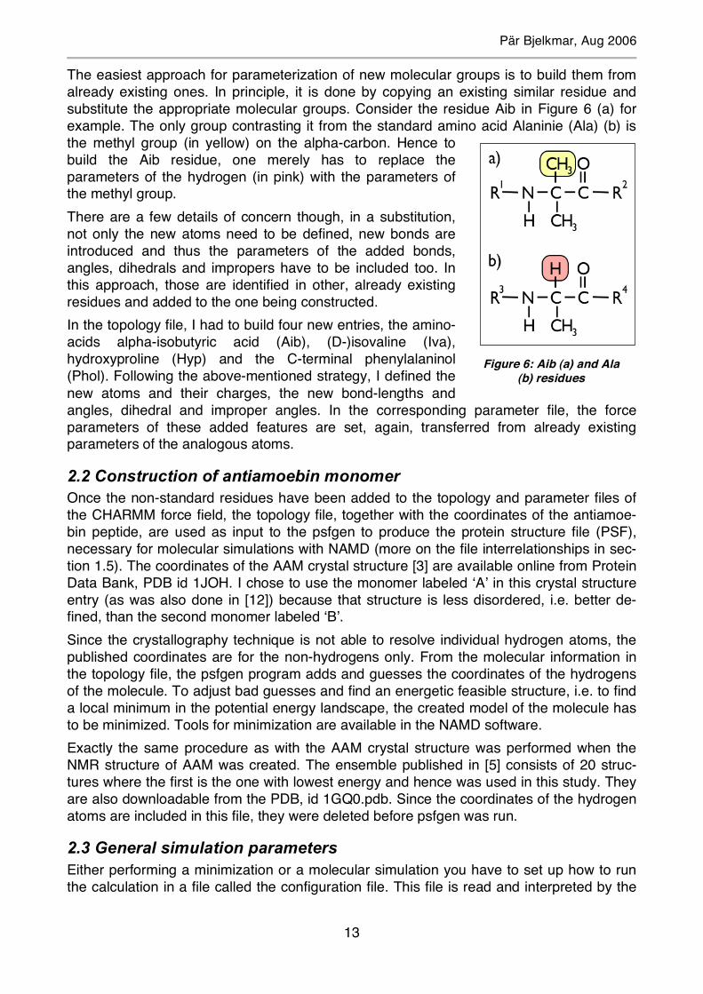
The easiest approach for parameterization of new molecular groups is to build them from already existing ones. In principle, it is done by copying an existing similar residue and substitute the appropriate molecular groups. Consider the residue Aib in Figure 6 (a) for example. The only group contrasting it from the standard amino acid Alaninie (Ala) (b) is the methyl group (in yellow) on the alpha-carbon. Hence to build the Aib residue, one merely has to replace the parameters of the hydrogen (in pink) with the parameters of the methyl group. There are a few details of concern though, in a substitution, not only the new atoms need to be defined, new bonds are introduced and thus the parameters of the added bonds, angles, dihedrals and impropers have to be included too. In this approach, those are identified in other, already existing residues and added to the one being constructed. In the topology file, I had to build four new entries, the amino-acids alpha-isobutyric acid (Aib), (D-)isovaline (Iva), hydroxyproline (Hyp) and the C-terminal phenylalaninol (Phol). Following the above-mentioned strategy, I defined the new atoms and their charges, the new bond-lengths and angles, dihedral and improper angles. In the corresponding parameter file, the force parameters of these added features are set, again, transferred from already existing parameters of the analogous atoms.
2.2 Construction of antiamoebin monomer Once the non-standard residues have been added to the topology and parameter files of the CHARMM force field, the topology file, together with the coordinates of the antiamoe-bin peptide, are used as input to the psfgen to produce the protein structure file (PSF), necessary for molecular simulations with NAMD (more on the file interrelationships in sec-tion 1.5). The coordinates of the AAM crystal structure [3] are available online from Protein Data Bank, PDB id 1JOH. I chose to use the monomer labeled ‘A’ in this crystal structure entry (as was also done in [12]) because that structure is less disordered, i.e. better de-fined, than the second monomer labeled ‘B’. Since the crystallography technique is not able to resolve individual hydrogen atoms, the published coordinates are for the non-hydrogens only. From the molecular information in the topology file, the psfgen program adds and guesses the coordinates of the hydrogens of the molecule. To adjust bad guesses and find an energetic feasible structure, i.e. to find a local minimum in the potential energy landscape, the created model of the molecule has to be minimized. Tools for minimization are available in the NAMD software. Exactly the same procedure as with the AAM crystal structure was performed when the NMR structure of AAM was created. The ensemble published in [5] consists of 20 struc-tures where the first is the one with lowest energy and hence was used in this study. They are also downloadable from the PDB, id 1GQ0.pdb. Since the coordinates of the hydrogen atoms are included in this file, they were deleted before psfgen was run.
2.3 General simulation parameters Either performing a minimization or a molecular simulation you have to set up how to run the calculation in a file called the configuration file. This file is read and interpreted by the
Figure 6: Aib (a) and Ala (b) residues
Pär Bjelkmar, Aug 2006
14
NAMD program. There are many different types of parameters in the configuration file; some are dealing with the output, others with specific methods used for the calculation and still others are parameters defining the environment of the system, e.g. temperature and pressure. The parameter file of the CHARMM force field is also required because it con-tains the parameters of the energy potential function in Eq. 4. To avoid tiresome repetition of the configuration file parameters of the simulations studied in this work, I chose to specify those whose values are staying constant throughout the dif-ferent runs in this section. If any other values are used, this will be indicated in the part corresponding to that simulation. In many cases of a simulation’s details, there are several options of which methods to use. All these methods and their parameters are specified in the current version of the NAMD user’s guide [20]. References to relevant publications are also available. A time step of 1 femtosecond was used for simulation integration. Bonded interactions were calculated every integration step whereas the more cumbersome non-bonded inter-actions were calculated only periodically as described below. 1-4 bonded interactions also contributed to the non-bonded term. The cutoff distance for the van der Waals interactions was 12 Å and a switching function with cutoff 10 Å was used for smooth truncation. Full electrostatic interactions were con-sidered only where the particle mesh Ewald method (PME) was used (see specification in corresponding section). If that was not the case, they were smoothly truncated at the cutoff distance as the van der Waal interactions. When full electrostatic interactions are consid-ered they are never truncated. In these cases the value of the cutoff instead stands for the local interaction distance. Within this distance, the Coulomb interactions were evaluated in every other time step and atom pairs separated by greater distances contributed every fourth time step. Both methods use the multistep integration method implemented in NAMD. The pair list used for optimizing pair-wise distance calculations considers all pairs within 13.5 Å of each other. Temperature control was accomplished by Langevin dynamics with a damping coefficient of 5/ps for an initial phase of the simulation (to minimize the effect of local temperature fluctuations due to bad contacts in the heterogeneous system). After some later point it was decreased to a more realistic value of 1/ps. The temperature target was 310 K in all calculations. The Nosé-Hoover method for pressure control was used in simulations of the NPT ensemble with a pressure target of 1.01325 bar (1 atm). Periodic boundary conditions were used exclusively.
2.4 Validation of monomer model One crucial point in molecular modeling is to compare the theoretical model with experimental data to verify that it is sound. In my case one immediate control is to compare the structure generated by the software to the published crystal structure. In so doing, it is possible to test whether the structural definitions of the non-standard residues added in the topology file are correct. The next step is to investigate how the built molecule behaves in different environments. In this way the force field is tested rather than simply the structural properties. The AAM monomer was studied in hexane, methanol and in a palmitoyloleoylphosphatidylcholine (POPC) bilayer. These three systems are all heterogeneous since they consist of more than one type of molecules. To construct the two former liquid environments, one approach is to start by building an appropriately big
Pär Bjelkmar, Aug 2006
15
box of the solution molecules. They should surround the solute completely and form a shielding “cushion” so that mirror images of the solute in the periodic system not unwontedly interact with each other. When the solute was added no atom in any molecule of the solution was allowed to be located within a certain distance (also user-defined, typically ~1 Å) from the solute. This is of course to avoid unnatural overlapping of molecules. The approach was also used later when inserting the transmembrane AAM molecule(s) in lipid bilayer(s). There is a tool in VMD for automatic construction of systems of water with arbitrary size, having “physiological” density (~0.033 water molecules/Å3) and molecular arrangement. Modification of such a system could function as a foundation for other systems, as in the construction of the methanol box. The plug-in tool is called solvate and is accessible both from the menu of the program and from the Tk(/Tcl) console. VMD also has a tool for automatic construction of membrane-water systems. The user specifies the size of the membrane patch and the lipid species. The program itself adds water to the system so that the lipid head groups are completely solvated. More water can be added “manually” if needed. Fortunately, POPC is one of only two lipid options available. Molecular dynamics trajectories were created for all three systems according to the descriptions in the following parts. One way to study these trajectories is to monitor how the secondary structure of the peptide evolves through time and thus investigate how stable the molecule is in the current environment. Conveniently, there is also a built in tool in VMD called “Timeline” for calculating such features. The fundamental secondary structure prediction algorithm used is STRIDE [21].
2.4.1 AAM in hexane Coordinates of a pre-equilibrated hexane box of size 47x47x51 Å at 300 K were kindly provided by Michael Wilson. Since the desired temperature was slightly higher, I ran an NPT simulation at 310 K to let the volume of the system adjust to the new temperature. This system was going to be used together with the AAM molecule and hence the hexane topology file, from the toppar_all27_lipid_model file in the stream subdirectory of the CHARMM force field download package, was added to my extended topology file (no changes in the corresponding parameter file is necessary since the atom species of a methanol molecule belong to the already parameterized ones). The coordinate file was fed to psfgen and together with this new topology file the program built the protein structure file. The files of the AAM crystal structure and the hexane box were then combined to form the heterogeneous system. In order to let the hexane molecules arrange themselves around the inserted helix, the first minimization was performed with the AAM atoms fixed at their original positions. After 1000 steps of conjugate minimization the energy had decreased to a stable value and the step length of the minimization indicated that the configuration had reached a local minimum. The restraints on the atoms were thereafter released and a new minimization of 1000 steps was run for relaxation of the complete system. Again, a longer run was not necessary. A NPT simulation of 3 ps was performed to allow the volume of the system to adjust to the inserted peptide. Finally, a 1.5 ns long NVT simulation was run, used for studying the stability of the helical molecule.
2.4.2 AAM in methanol To create the methanol system, a water box of size 50x50x50 Å was built with the solvate plug-in. A quick calculation and comparison of the expected number of water and methanol
Pär Bjelkmar, Aug 2006
16
molecules/Å3 was done. A methanol system under the same conditions has approximately half the number of molecules/Å3 (0.01488 versus 0.03342 respectively) and consequently every other water molecule in the system’s coordinate file (the PDB-file) was deleted. This is not a critical step though, since the system will be equilibrated later and hence will have the chance to adjust to its proper density. The remaining water molecules were manually edited so that one of the hydrogens was converted to a methyl carbon species and the other to a hydroxyl oxygen. The methanol topology definition from the CHARMM topology file top_all30_cheq_prot was added to my extended topology file. The edited coordinate file and the new topology file were used as input to the psfgen and again, the protein structure- and the coordinate files were built. As always when psfgen has been used, the acquired system has to be minimized to allow for bad local arrangements to adjust themselves into an energetic relaxed state. It was done in a 3000 steps conjugate minimization. A NPT simulation of this system was run so the equilibrium volume of the system was reached. It was completed in a 540 ps long simulation, using full electrostatic interactions in the form of PME with grid size 64x64x64. The NMR structure of lowest energy was inserted into the methanol box. In the process methanol molecules within 0.8 Å was deleted. Minimization, first with the peptide held fixed, was carried out for a total of 5000 steps. A short simulation in which N, P, and T were held constant followed these, again to allow the volume of the system to adjust to the new state with the AAM peptide added. PME was used as before. The AAM molecule was found to be less stable in this solution than in the hexane so a longer equilibrium simulation of almost 20 ns was run. Another analysis was also performed using the crystal structure of AAM as starting structure instead. Starting from the equilibrated methanol box, the helix was added, again deleting methanol molecules within 0.8 Å of the peptide. Following minimization and NPT-simulation, the simulation in the NVT ensemble was run for 20 ns, where the AAM molecule was held fixed during the initial 2.4 ns.
2.4.3 AAM in POPC lipid bilayer The membrane plug-in tool in VMD was used initially to construct a 50x50 Å big patch of POPC lipid bilayer surrounded by water. The crystal structure of the AAM helix was sub-sequently moved and inserted in a transmembrane position; the general axis of the mole-cule approximately perpendicular to the membrane surface. After two minimization runs, first with fixated helix for 1200 steps followed by an unrestrained calculation of 2400 steps, the system was run in NPT for 4.4 ns. PME with grid size 64x64x64 was used for the elec-trostatic interactions. This ensemble is most commonly used in membrane systems since the pressure is a more natural parameter to control in these (compared to the volume).
2.5 Construction of transmembrane channel Now when the individual helix has been studied, we turn to building models of the helical bundles forming the AAM transmembrane channel. In this work, I have studied both an octameric and a tetrameric bundle of helices (consisting of eight and four helices respectively). The octameric model considered is the structure O’Reilley and Wallace presented in 2003, whereas the tetrameric model was constructed using the their approach.
Pär Bjelkmar, Aug 2006
17
2.5.1 Octameric bundle A PDB coordinate file of the eight-helix bundle was kindly provided by O’Reilley and Wallace. The psfgen program responsible for the genesis of the PSF file has a restriction in that distinct peptide chains have to be provided in separate PDB files. To perform such a task starting from the complete PDB file is easy in VMD’s Tk console. At the same time hydrogens were deleted. In the standard way, psfgen generates a PSF and a PDB file, the latter including the coordinates of the complete channel model. This structure was inserted in a 100x100 Å patch of POPC bilayer (again, with solvated head groups), built with the VMD membrane package. The two structures are aligned in such a way that the direction of the channel (along the z-axis) was perpendicular to the membrane-water surface. In addition to POPC molecules having at least one atom within 0.8 Å of the channel, all lipids enclosed by the bundle were deleted. This procedure removed 54 molecules, not necessarily symmetrically in both monolayers. Additional water molecules were added to this system with VMD’s solvate package, totally forming a water slab with a thickness of ~26 Å. Before ions were added to this heterogeneous system, it had to be minimized and run for a while so the local anomalies resulting from the deletion of POPC molecules could be rectified. The system was run with a periodic box having initial dimensions 100x100x70 Å. The PME method with a grid size of 128x128x128 was used to account for the electrostatical interactions (note that the system has a zero net charge). First, a minimization of 6000 steps, holding the peptide channel fixed, was performed. Releasing the restraints, an additional 6000 steps minimization followed. The channel was restrained again and run in the NPT ensemble for 3 ns, in particular because the water molecules had to have time to diffuse into the vacuum of the pore. During this relaxation time, the temperature-damping coefficient was held at the relatively high value of 5/ps to be able to quickly suppress local temperature fluctuations that might occur in such an early stage of the equilibrium process. Ions were added to the system using the autoionize tool in VMD. A KCl concentration of 0.5 M was created. In brief, this is accomplished by substituting the appropriate number of randomly selected water molecules with ions. This final system consists of totally 51421 atoms. Again, I was careful of local bad contacts introduced by the ionization, so the channel was fixed during the first 0.96 ns of the subsequent (NPT) simulation. For the remaining part of the simulation the system was run with an unrestrained AAM channel and a temperature-damping coefficient of 1/ps. During the simulation structures were sampled every 10 ps and the resulting trajectory corresponds to 22.8 ns of simulation (excluding minimizations). Another indicator of how the structure of a molecule evolves over time, besides the secondary structure analysis, is to calculate the root mean square deviation (RMSD). It measures the average distance between a selection of atoms compared to the corresponding atoms in a reference structure. Note that this method does not incorporate relative molecular motion because the two structures are superimposed before the calculation is performed. Atoms typically considered are the ones forming the backbone of the peptide since they are much less affected by temporal structural fluctuations, prominent in the side chains. As reference structure, the initial configuration is typically used and calculating the RMSD of the following states yields the time evolution. When plotting the RMSD, an unavoidable increase is expected in the beginning but as time goes by, the curve should flatten out and stabilize (even though small fluctuations still naturally will occur) when the structure has equilibrated.
Pär Bjelkmar, Aug 2006
18
Such a RMSD analysis, using the backbone atoms of the AAM helices as selection and the starting structure as the reference structure, was performed for the trajectory of the eight-helix system. To investigate the structure of the pore of the channel, I used the free software HOLE [22]. It basically probes the pore with spheres, calculating the radius of the hole at points along the general direction of the channel. The last structure in the simulation was used. The maximum radius of the probe was set to 13 Å. When it is exceeded in both ends of the pore the calculation terminates. The output data was plotted in VMD with a plug-in written by Andriy Anishkin [23]. Yet another script written by Andriy was used for extracting hydrogen bonds from the trajectory [24], used for studying the hydrogen-bonding pattern in the bundle. First, the number of interhelical hydrogen bonds (i.e. hydrogen bonds formed in between residues belonging to distinct helices) was plotted for every tenth sampled time point in the simulation. After a rather arbitrary cutoff time of 10 ns (used because of the more easily defined cutoff in the corresponding tetrameric analysis), counts of which types of interhelical hydrogen bonds present were performed.
2.5.2 Tetrameric bundle As I indicated previously, the tetrameric channel model was created according to the approach used by O’Reilley and Wallace in 2003. The eight-helix model was used as starting point. Every other helix was then deleted and the remaining four were moved closer together, in the xy-plane, toward the imaginary z-axis penetrating the channel. They were symmetrically translated in such a way that the Gln 11 side chains pointing inward, approximately formed a stabilizing ring structure analogous to its larger sister model. A copy of the original POPC bilayer from the building of the octameric system was used for tetrameric channel insertion. The 30 POPC phospholipids having at least one atom within a distance of 0.8 Å of the channel were deleted. Additional water was added, forming a total water thickness of approximately 26 Å as in the octameric case. This system was minimized and run for 2 ns in NPT before the ionization occurred. PME with a grid size 128x128x128 was used. The periodic box was initially having dimensions of 100x100x70 Å. 6000 steps of minimization with the channel held fixed were followed by an additional 6000 steps with released restrains. After 2 ns of NPT simulation where the channel was held in its starting conformation, ions were added with the autoionize tool. Again, a KCl concentration of 0.5 M was created. Minimizations of 2*6000 followed before the actual NPT equilibrium run was started. During the first 0.96 ns the channel was held fixed and the Langevin damping coefficient was held at the higher 5/ps. Because of reasons discussed in chapter 4, one potassium ion was restrained to a distance of 4 Å from the average coordinates of the alpha-carbons of the Gln 11 residues for the first 8.64 ns. A built-in feature of NAMD, allowing imposing forces on atoms, was used to achieve this. Once the ion diffuses away from the window between one and the next integration steps, a force, dependent on the quadratic distance of the ion from the window border, is applied on the ion pushing it back into the window. A force constant of 20 kcal/mol For the following 21.00 ns the system was run without any restraints at all adding up to a total trajectory of length 29.64 ns. Outputs from the simulation were sampled every 10 ps. The same analyses as in the octameric study were performed: RMSD calculation with respect to the starting structure, investigation of pore size of the last structure in the
Pär Bjelkmar, Aug 2006
19
simulation and the interhelical hydrogen-bonding pattern. In addition, an analysis of the availability of carbonyl oxygens in the narrow C-terminal part of the channel was performed (the rationale of this analysis is also elaborated in chapter 4). Only carbonyl oxygens pointing inwards in the channel were considered. These are the carbonyl oxygens of residues Hyp 10, Gln 11 and Aib 14, denoted Hyp 10:O, Gln 11:O and Aib 14:O. To assess the availability of these groups, one needs to count how many of them are occupied in either interhelical or intrahelical H-bonds. Again, the same time window of the simulation was considered, 10.00-29.64 ns.
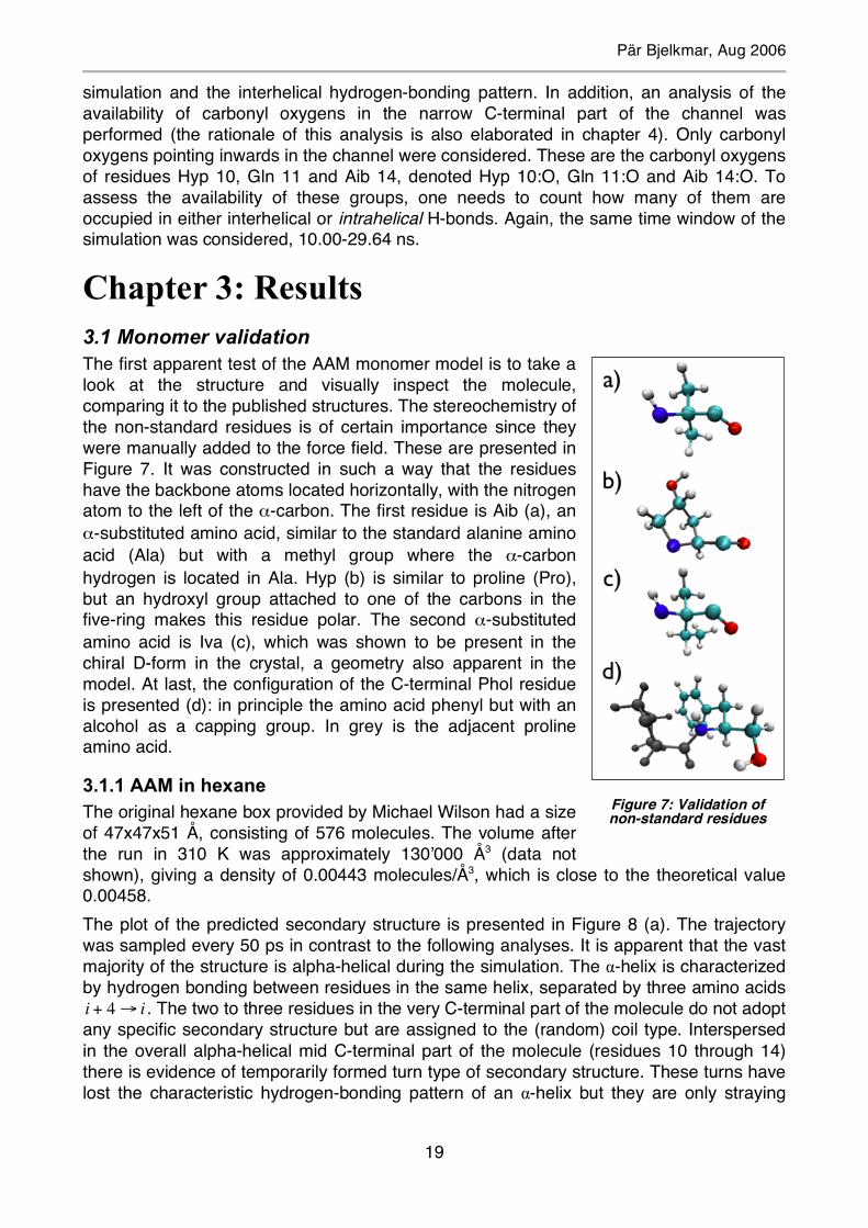
Chapter 3: Results 3.1 Monomer validation The first apparent test of the AAM monomer model is to take a look at the structure and visually inspect the molecule, comparing it to the published structures. The stereochemistry of the non-standard residues is of certain importance since they were manually added to the force field. These are presented in Figure 7. It was constructed in such a way that the residues have the backbone atoms located horizontally, with the nitrogen atom to the left of the α-carbon. The first residue is Aib (a), an α-substituted amino acid, similar to the standard alanine amino acid (Ala) but with a methyl group where the α-carbon hydrogen is located in Ala. Hyp (b) is similar to proline (Pro), but an hydroxyl group attached to one of the carbons in the five-ring makes this residue polar. The second α-substituted amino acid is Iva (c), which was shown to be present in the chiral D-form in the crystal, a geometry also apparent in the model. At last, the configuration of the C-terminal Phol residue is presented (d): in principle the amino acid phenyl but with an alcohol as a capping group. In grey is the adjacent proline amino acid.
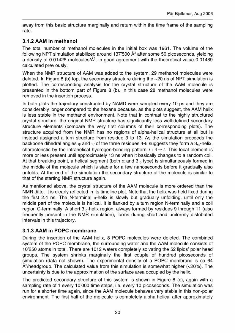
3.1.1 AAM in hexane The original hexane box provided by Michael Wilson had a size of 47x47x51 Å, consisting of 576 molecules. The volume after the run in 310 K was approximately 130’000 Å3 (data not shown), giving a density of 0.00443 molecules/Å3, which is close to the theoretical value 0.00458. The plot of the predicted secondary structure is presented in Figure 8 (a). The trajectory was sampled every 50 ps in contrast to the following analyses. It is apparent that the vast majority of the structure is alpha-helical during the simulation. The α-helix is characterized by hydrogen bonding between residues in the same helix, separated by three amino acids
!
i + 4" i . The two to three residues in the very C-terminal part of the molecule do not adopt any specific secondary structure but are assigned to the (random) coil type. Interspersed in the overall alpha-helical mid C-terminal part of the molecule (residues 10 through 14) there is evidence of temporarily formed turn type of secondary structure. These turns have lost the characteristic hydrogen-bonding pattern of an α-helix but they are only straying
Figure 7: Validation of non-standard residues
Pär Bjelkmar, Aug 2006
20
away from this basic structure marginally and return within the time frame of the sampling rate.
3.1.2 AAM in methanol The total number of methanol molecules in the initial box was 1961. The volume of the following NPT simulation stabilized around 137’500 Å3 after some 50 picoseconds, yielding a density of 0.01426 molecules/Å3, in good agreement with the theoretical value 0.01489 calculated previously. When the NMR structure of AAM was added to the system, 29 methanol molecules were deleted. In Figure 8 (b) top, the secondary structure during the ~20 ns of NPT simulation is plotted. The corresponding analysis for the crystal structure of the AAM molecule is presented in the bottom part of Figure 8 (b). In this case 28 methanol molecules were removed in the insertion process. In both plots the trajectory constructed by NAMD were sampled every 10 ps and they are considerably longer compared to the hexane because, as the plots suggest, the AAM helix is less stable in the methanol environment. Note that in contrast to the highly structured crystal structure, the original NMR structure has significantly less well-defined secondary structure elements (compare the very first columns of their corresponding plots). The structure acquired from the NMR has no regions of alpha-helical structure at all but is instead assigned a turn structure from residue 3 to 13. As the simulation proceeds the backbone dihedral angles ϕ and ψ of the three residues 4-6 suggests they form a 310-helix, characteristic by the intrahelical hydrogen-bonding pattern
!
i + 3" i . This local element is more or less present until approximately 13 ns when it basically changes to a random coil. At that breaking point, a helical segment (both α and 310 type) is simultaneously formed in the middle of the molecule which is stable for a few nanoseconds before it gradually also unfolds. At the end of the simulation the secondary structure of the molecule is similar to that of the starting NMR structure again. As mentioned above, the crystal structure of the AAM molecule is more ordered than the NMR ditto. It is clearly reflected in its timeline plot. Note that the helix was held fixed during the first 2.4 ns. The N-terminal α-helix is slowly but gradually unfolding, until only the middle part of the molecule is helical. It is flanked by a turn region N-terminally and a coil region C-terminally. A short 310-helix region, always formed by residues 9 through 11 (also frequently present in the NMR simulation), forms during short and uniformly distributed intervals in this trajectory.
3.1.3 AAM in POPC membrane During the insertion of the AAM helix, 8 POPC molecules were deleted. The combined system of the POPC membrane, the surrounding water and the AAM molecule consists of 10’250 atoms in total. There are 1012 waters completely solvating the 52 lipids’ polar head groups. The system shrinks marginally the first couple of hundred picoseconds of simulation (data not shown). The experimental density of a POPC membrane is ca 64 Å2/headgroup. The calculated value from this simulation is somewhat higher (<20%). The uncertainty is due to the approximation of the surface area occupied by the helix. The predicted secondary structure of this system is shown in Figure 8 (c), again with a sampling rate of 1 every 10’000 time steps, i.e. every 10 picoseconds. The simulation was run for a shorter time again, since the AAM molecule behaves very stable in this non-polar environment. The first half of the molecule is completely alpha-helical after approximately
Pär Bjelkmar, Aug 2006
21
2.8 ns, when residue 1 and 2 join the downstream residues. The C-terminal end of this helical segment (residues 9-11) is continuously switching between the two helical types. These conformational rearrangements occur on a timescale of the sampling rate.
Following this helix, the N-terminal part of the molecule consists of a short turn and coil region, sequentially.
Figure 8: Secondary structure of AAM monomers in hexane (a), methanol (b) and POPC bilayer (c)
Pär Bjelkmar, Aug 2006
22
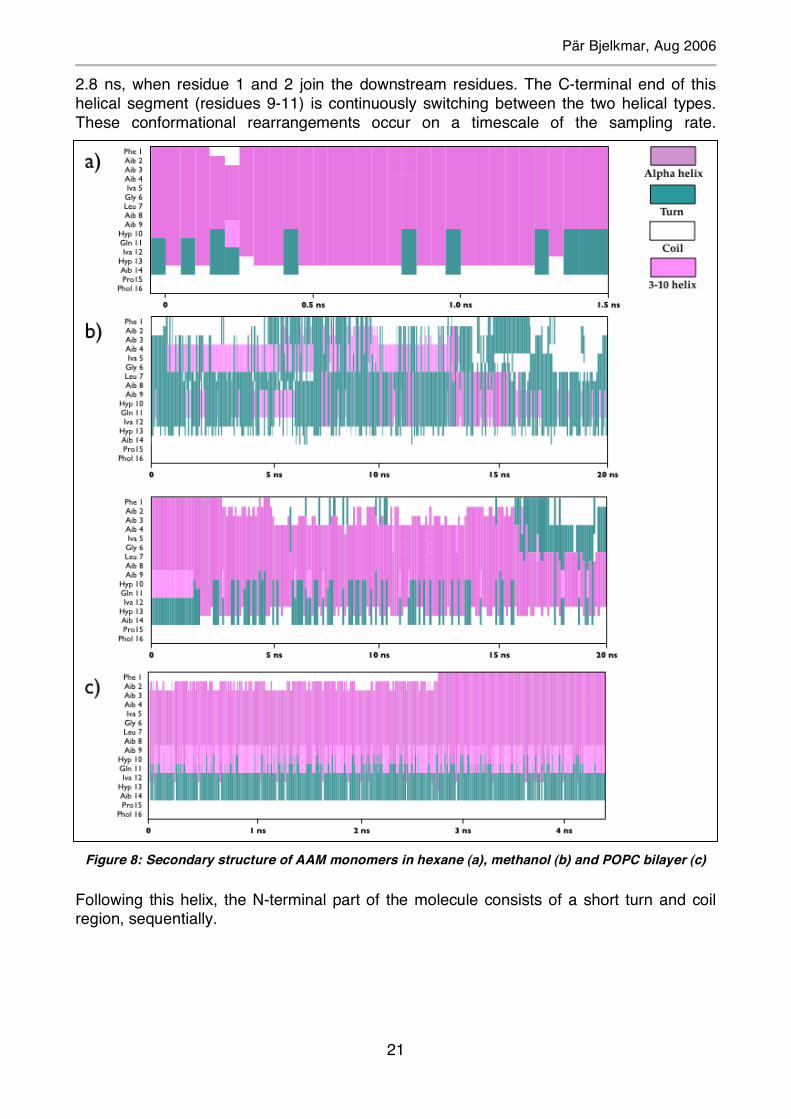
3.2 Octameric model The first NPT simulation of the unionized system allowed for the water molecules to diffuse into the vacuum of the pore. Moreover, the lipids surrounding the channel had time to fill the gaps in the membrane caused by the deletion of sister molecules. As the water starts filling the big empty space in the channel, the ones in the periphery of the periodic box replaces them and the system consequently shrinks significantly in the z-dimension. In the x and y dimensions though, the periodic box is almost as big as it was before the simulations started (as was also the case with the AAM monomer inserted in the POPC membrane discussed above). After the ionization of the system it consists of 51’421 atoms, divided among 220 POPC molecules, 6’637 waters, 62 ions (31 of each species) and the AAM channel. To investigate if the surface of the membrane has an appropriate density, the area occupied by the channel need to be subtracted from the area of the periodic box in the xy-plane. The box size fluctuates over the simulation so a few randomly selected time points are considered (after 10 ns when the system has had time to equilibrate some). In this case, as opposed
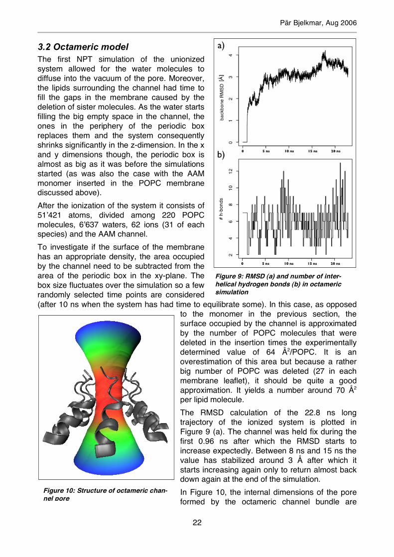
to the monomer in the previous section, the surface occupied by the channel is approximated by the number of POPC molecules that were deleted in the insertion times the experimentally determined value of 64 Å2/POPC. It is an overestimation of this area but because a rather big number of POPC was deleted (27 in each membrane leaflet), it should be quite a good approximation. It yields a number around 70 Å2 per lipid molecule. The RMSD calculation of the 22.8 ns long trajectory of the ionized system is plotted in Figure 9 (a). The channel was held fix during the first 0.96 ns after which the RMSD starts to increase expectedly. Between 8 ns and 15 ns the value has stabilized around 3 Å after which it starts increasing again only to return almost back down again at the end of the simulation. In Figure 10, the internal dimensions of the pore formed by the octameric channel bundle are
Figure 9: RMSD (a) and number of inter-helical hydrogen bonds (b) in octameric simulation
Figure 10: Structure of octameric chan-nel pore
Pär Bjelkmar, Aug 2006
23
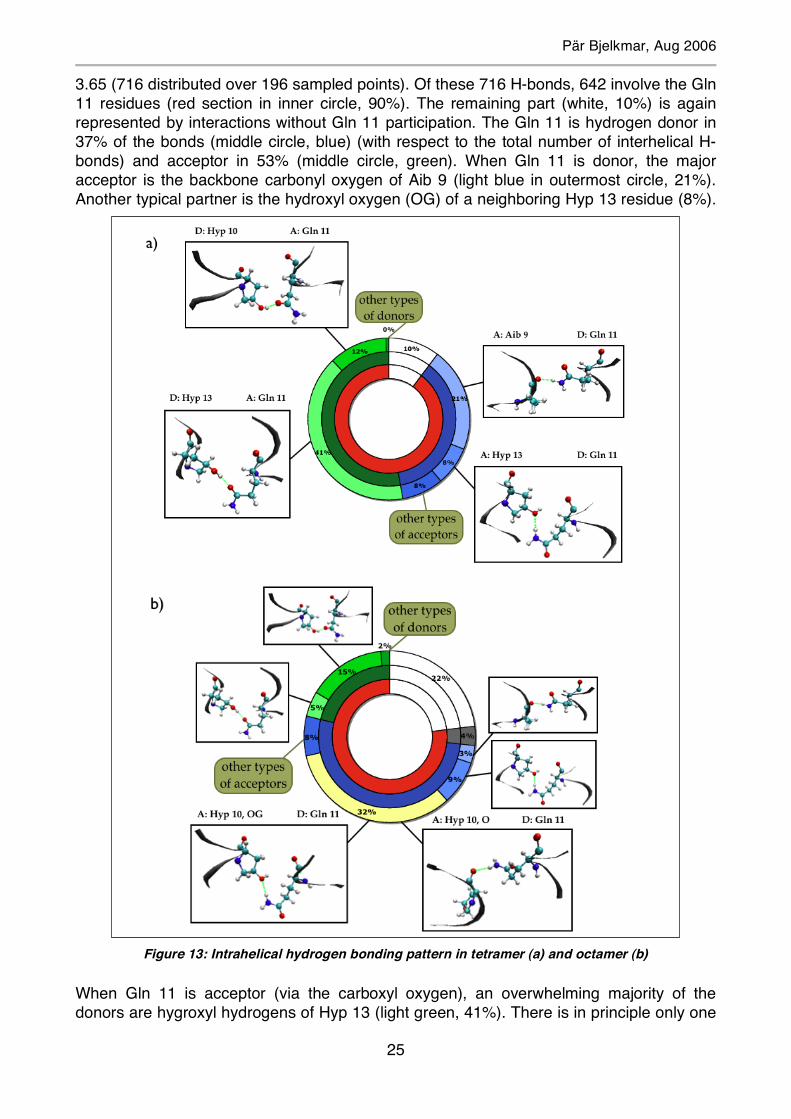
presented. The color-code spans from the minimum radius in red, 5.005 Å, through yellow and green to blue at the (user-set) maximum radius of 13 Å. The final analysis for both the octamer and the tetramer is the analysis of the interhelical hydrogen-bonding pattern. Note, from now on all hydrogen bonds I am referring to in this section are interhelical, unless stated otherwise. First, the time evolution of the number of such bonds is presented in Figure 9 (b), sampled every 100 ps. No overall increasing trend is obvious and a cutoff, after which the number has stabilized, is quite arbitrary. After approximately 10 ns the pattern is somewhat different and since this is the cutoff indicated by the corresponding tetrameric analysis it was used here too. Statistics of the types of hydrogen bonds collected after the cutoffs of both octamer and tetramer are visualized in the doughnut graphs in Figure 13 (because of layout-technical reasons the tetrameric graph was placed in (a) and the octameric in (b)). Consider the statistics of the octamer in (b). The total number of interhelical hydrogen bonds present after the cutoff of 10 ns is 763 (full circle, 100%), giving an average number of 5.96 (763/128) H-bonds per sampled time point. The innermost circle separates the H-bonds involving Gln 11 residues (in red, rounded to 78%) from the others (in white 22%). The interactions not involving Gln 11 are substantially interhelical hydrogen bonds between Phol 16 and Pro 15 or Aib 14. The second circle divides the Gln 11 section of the first circle into H-bonds where this amino acid has the function of (hydrogen) donor (in dark blue, 52 %), acceptor (in dark green, 22%), and both donor and acceptor in Gln 11-Gln 11 hydrogen bonds (gray, 4%). In the outermost circle the explicit hydrogen bonding partners of the Gln 11 residues are depicted. The biggest type is the Gln 11-Hyp 10 interactions, where Gln 11 is donor and the carbonyl or hydroxyl oxygens, denoted O and OG respectively, of Hyp 10 are acceptors (in beige, 32%). Worth noting is that these H-bonds types are considerably fewer in the tetramer. The major donor, when Gln 11 is acceptor, is Hyp 10. A more complete comparison of the interhelical hydrogen bonding patterns of the octamer and the tetramer is available in chapter 4. ‘D’ is the notation for donor and ‘A’ is for acceptor in the textual specifications of hydrogen bonding pairs placed above the detailed molecular pictures. Neighboring helices are represented in gray/black. Note that the smaller pictures in the octameric graph (b), without accompanying text, are the same types of hydrogen bonds as the corresponding bigger pictures in (a).
3.3 Tetrameric model The unionized system with the added, extra water has to run a while so that the water has time to fill the empty pore of the channel. Following this 2 ns long NPT simulation the system is ionized, after which it consists of totally 53’629 atoms. Among these, there are 244 POPC molecules (134 atoms/molecule), 6’629 waters, 62 ions (31 K+ and 31 Cl-) and the remaining 984 atoms materialize the channel. The dimensions of the periodic box behave similarly to the eight-helix case; the z-dimension shrinks to the mid-fifties while the x, y dimensions only shrinks marginally. To assess the approximate surface density of the system it is probably, again, best to use the value of the surface density available in the literature (64 Å2/POPC molecule) and the number of deleted POPC molecules in the insertion of the channel for the approximation of the area occupied by the channel. The periodic box has a size of ca 96x96 Å. Subtracting 15*64 Å2 from this area and dividing the difference between the 122 POPC molecules in one membrane leaflet yields a surface
Pär Bjelkmar, Aug 2006
24
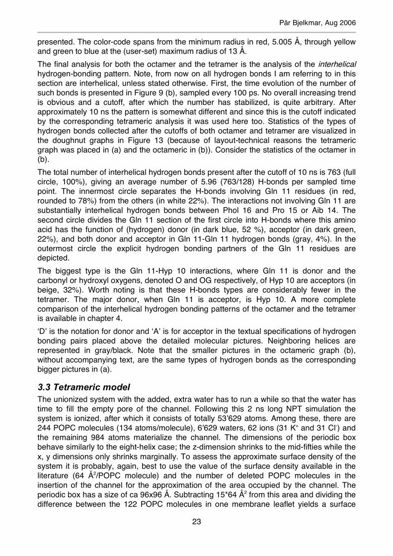
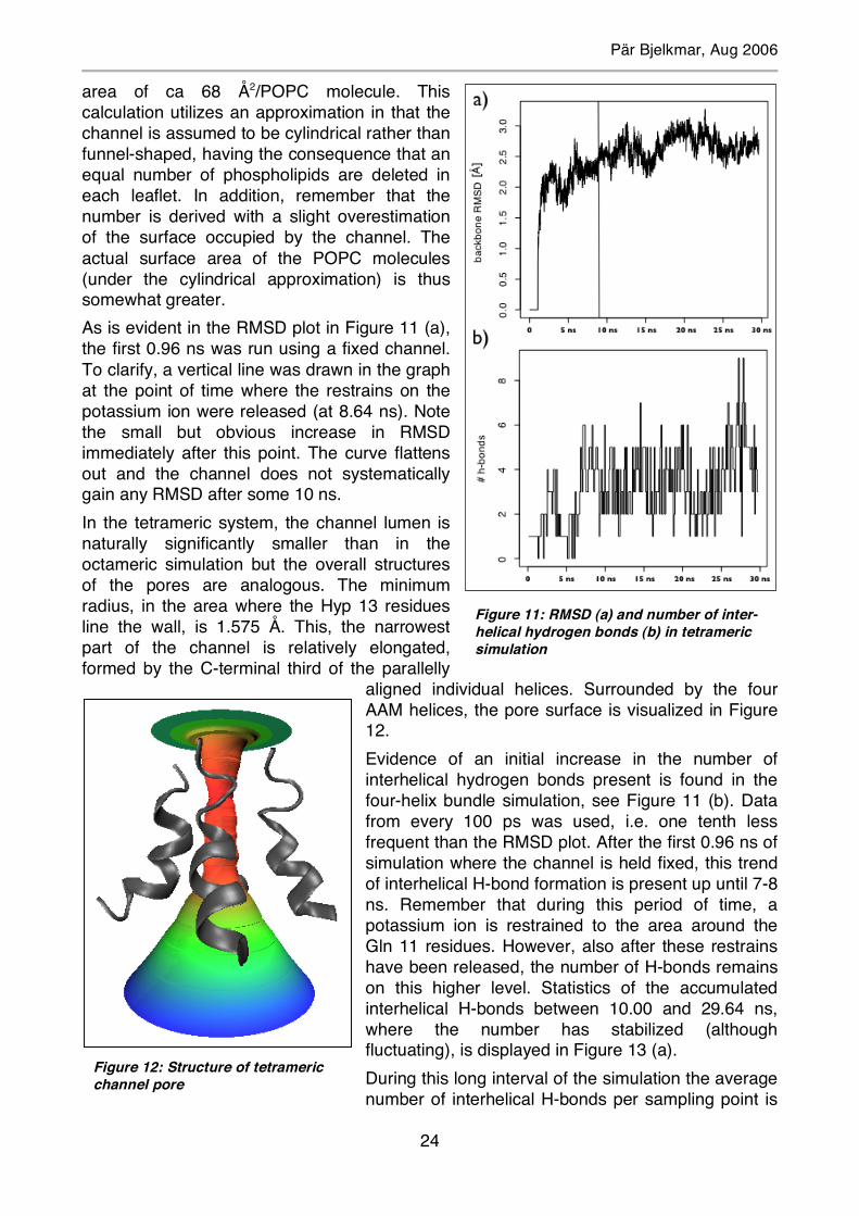
area of ca 68 Å2/POPC molecule. This calculation utilizes an approximation in that the channel is assumed to be cylindrical rather than funnel-shaped, having the consequence that an equal number of phospholipids are deleted in each leaflet. In addition, remember that the number is derived with a slight overestimation of the surface occupied by the channel. The actual surface area of the POPC molecules (under the cylindrical approximation) is thus somewhat greater. As is evident in the RMSD plot in Figure 11 (a), the first 0.96 ns was run using a fixed channel. To clarify, a vertical line was drawn in the graph at the point of time where the restrains on the potassium ion were released (at 8.64 ns). Note the small but obvious increase in RMSD immediately after this point. The curve flattens out and the channel does not systematically gain any RMSD after some 10 ns. In the tetrameric system, the channel lumen is naturally significantly smaller than in the octameric simulation but the overall structures of the pores are analogous. The minimum radius, in the area where the Hyp 13 residues line the wall, is 1.575 Å. This, the narrowest part of the channel is relatively elongated, formed by the C-terminal third of the parallelly
aligned individual helices. Surrounded by the four AAM helices, the pore surface is visualized in Figure 12. Evidence of an initial increase in the number of interhelical hydrogen bonds present is found in the four-helix bundle simulation, see Figure 11 (b). Data from every 100 ps was used, i.e. one tenth less frequent than the RMSD plot. After the first 0.96 ns of simulation where the channel is held fixed, this trend of interhelical H-bond formation is present up until 7-8 ns. Remember that during this period of time, a potassium ion is restrained to the area around the Gln 11 residues. However, also after these restrains have been released, the number of H-bonds remains on this higher level. Statistics of the accumulated interhelical H-bonds between 10.00 and 29.64 ns, where the number has stabilized (although fluctuating), is displayed in Figure 13 (a). During this long interval of the simulation the average number of interhelical H-bonds per sampling point is
Figure 11: RMSD (a) and number of inter-helical hydrogen bonds (b) in tetrameric simulation
Figure 12: Structure of tetrameric channel pore
Pär Bjelkmar, Aug 2006
25
3.65 (716 distributed over 196 sampled points). Of these 716 H-bonds, 642 involve the Gln 11 residues (red section in inner circle, 90%). The remaining part (white, 10%) is again represented by interactions without Gln 11 participation. The Gln 11 is hydrogen donor in 37% of the bonds (middle circle, blue) (with respect to the total number of interhelical H-bonds) and acceptor in 53% (middle circle, green). When Gln 11 is donor, the major acceptor is the backbone carbonyl oxygen of Aib 9 (light blue in outermost circle, 21%). Another typical partner is the hydroxyl oxygen (OG) of a neighboring Hyp 13 residue (8%).
When Gln 11 is acceptor (via the carboxyl oxygen), an overwhelming majority of the donors are hygroxyl hydrogens of Hyp 13 (light green, 41%). There is in principle only one
Figure 13: Intrahelical hydrogen bonding pattern in tetramer (a) and octamer (b)
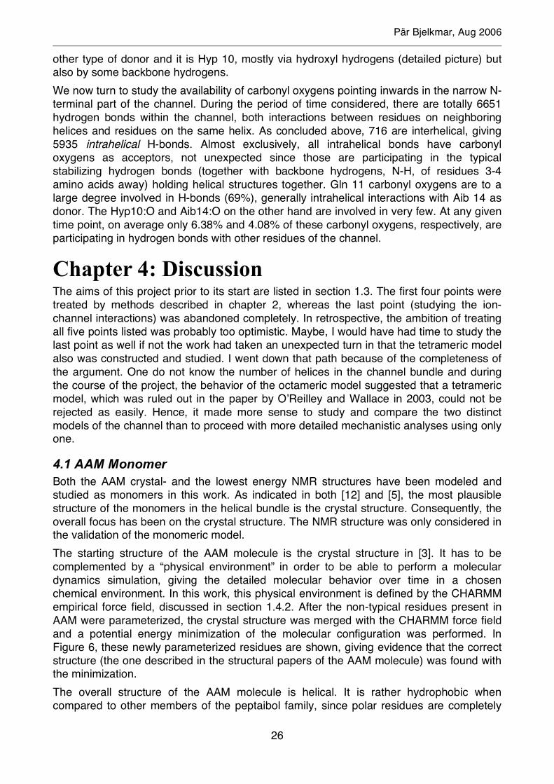
Pär Bjelkmar, Aug 2006
26
other type of donor and it is Hyp 10, mostly via hydroxyl hydrogens (detailed picture) but also by some backbone hydrogens. We now turn to study the availability of carbonyl oxygens pointing inwards in the narrow N-terminal part of the channel. During the period of time considered, there are totally 6651 hydrogen bonds within the channel, both interactions between residues on neighboring helices and residues on the same helix. As concluded above, 716 are interhelical, giving 5935 intrahelical H-bonds. Almost exclusively, all intrahelical bonds have carbonyl oxygens as acceptors, not unexpected since those are participating in the typical stabilizing hydrogen bonds (together with backbone hydrogens, N-H, of residues 3-4 amino acids away) holding helical structures together. Gln 11 carbonyl oxygens are to a large degree involved in H-bonds (69%), generally intrahelical interactions with Aib 14 as donor. The Hyp10:O and Aib14:O on the other hand are involved in very few. At any given time point, on average only 6.38% and 4.08% of these carbonyl oxygens, respectively, are participating in hydrogen bonds with other residues of the channel.
Chapter 4: Discussion The aims of this project prior to its start are listed in section 1.3. The first four points were treated by methods described in chapter 2, whereas the last point (studying the ion-channel interactions) was abandoned completely. In retrospective, the ambition of treating all five points listed was probably too optimistic. Maybe, I would have had time to study the last point as well if not the work had taken an unexpected turn in that the tetrameric model also was constructed and studied. I went down that path because of the completeness of the argument. One do not know the number of helices in the channel bundle and during the course of the project, the behavior of the octameric model suggested that a tetrameric model, which was ruled out in the paper by O’Reilley and Wallace in 2003, could not be rejected as easily. Hence, it made more sense to study and compare the two distinct models of the channel than to proceed with more detailed mechanistic analyses using only one.
4.1 AAM Monomer Both the AAM crystal- and the lowest energy NMR structures have been modeled and studied as monomers in this work. As indicated in both [12] and [5], the most plausible structure of the monomers in the helical bundle is the crystal structure. Consequently, the overall focus has been on the crystal structure. The NMR structure was only considered in the validation of the monomeric model. The starting structure of the AAM molecule is the crystal structure in [3]. It has to be complemented by a “physical environment” in order to be able to perform a molecular dynamics simulation, giving the detailed molecular behavior over time in a chosen chemical environment. In this work, this physical environment is defined by the CHARMM empirical force field, discussed in section 1.4.2. After the non-typical residues present in AAM were parameterized, the crystal structure was merged with the CHARMM force field and a potential energy minimization of the molecular configuration was performed. In Figure 6, these newly parameterized residues are shown, giving evidence that the correct structure (the one described in the structural papers of the AAM molecule) was found with the minimization. The overall structure of the AAM molecule is helical. It is rather hydrophobic when compared to other members of the peptaibol family, since polar residues are completely
Pär Bjelkmar, Aug 2006
27
missing in the N-terminal half of the molecule. Still, it forms an amphipathic molecule, with polar groups located particularly on the convex side of the helix. Hydrophilic side chains of Hyp 10 and Gln 11 are located on this phase as well as carbonyl oxygens of Gly 6 and Leu 7, both without intrahelical hydrogen bonding partners [12] (due to the imino acid Hyp lacking the corresponding hydrogen donor) and thus add to the polarity. Taking this hydrophobicity into account, one would expect the helix to be more stable in apolar environments such as hexane and when inserted in a lipid bilayer than the other peptaibol species. Two of the structural studies available, the crystal structure used and the NMR structures, used a methanol environment whereas the other crystal structure (almost identical to the first one) was determined in n-octanol. To test the monomeric model further before using it in building a model of the channel, investigations of its dynamic properties were conducted. Molecular dynamics simulations were run where the AAM model was inserted into three interesting environments. Hexane was chosen as polar environment since my coworkers at Ames already had worked in such systems. Methanol was used as the polar representative because it had been used in the structural papers. The AAM monomer was also inserted in a POPC (palmitoyloleoylphosphatidylcholine) membrane bilayer, in which the AAM molecule has been shown to form channels [8]. One way to monitor how the structure of the molecule behaves in a molecular dynamics trajectory is to investigate how the secondary structure of the molecule evolves through time. If secondary structure elements remain stable under extended periods of time, one could conclude that those local features are stable. However, one very important thing one has to take into account is the timescales on which different structural rearrangements occur. As seen in the secondary structure plots in Figure 8, fluctuations in the local structure are on a timescale of the sampling rate, i.e. tenths of picoseconds. When larger, more collective properties of protein complexes are considered, as channel gating for example, the timescales are several orders of magnitude longer, milliseconds in this particular case. The time averages responsible for experimental NMR are also acquired over timescales of milliseconds. Molecular dynamics trajectories of such great lengths are not technically possible to simulate with today’s methods and computers. Expectedly, the AAM molecule is very stable in the hexane environment (Figure 8 (a)). Stable in the sense that the molecule does not unfold (partly or totally) and remains similar to the starting structure. In the methanol environment however, both the NMR and crystal structures are considerable less stable. The former gradually unfolds until only the middle part of the molecule has anything but a random coil secondary structure after 20 ns of simulation. One important thing to have in mind here though is that the starting structure itself has a rather low fraction of residues participating in well-defined secondary structures (compared to the crystal structure for example), with not a single assigned α-helix region. In the simulation starting with the crystal structure in methanol solution, the molecule also gradually looses its secondary structure (the N-terminal α-helical region in this case). Only the middle part is still assigned to the α-helix type at the end of the simulation. In the rather big and complex membrane-water system the predicted secondary structure of the AAM molecule suggest a very stable molecule. This might not be very unexpected given the behavior in hexane above; the lipid side chains forming the large central part of the membrane are very hydrophobic. The AAM molecule remains a transmembrane helix throughout the simulation, i.e. the helix axis is approximately parallel to the normal of the membrane surface. This indicates that, at least the individual helices in the channel model will not be unstable and unfold.
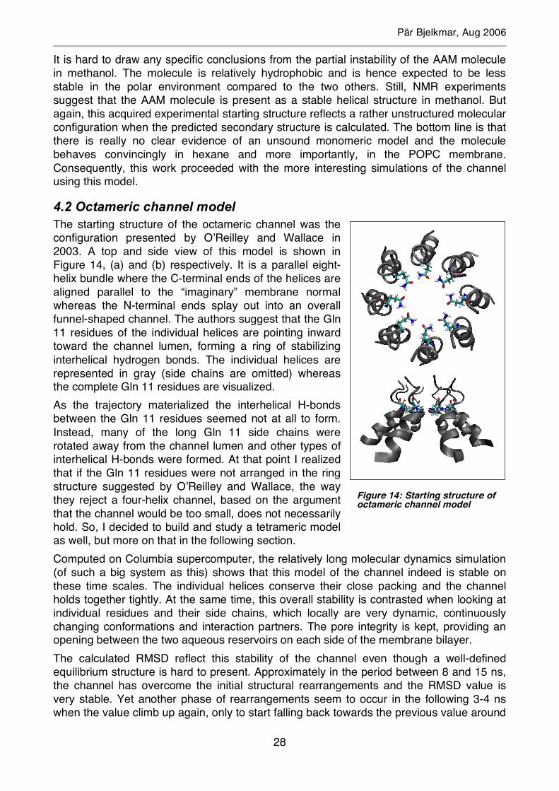
Pär Bjelkmar, Aug 2006
28
It is hard to draw any specific conclusions from the partial instability of the AAM molecule in methanol. The molecule is relatively hydrophobic and is hence expected to be less stable in the polar environment compared to the two others. Still, NMR experiments suggest that the AAM molecule is present as a stable helical structure in methanol. But again, this acquired experimental starting structure reflects a rather unstructured molecular configuration when the predicted secondary structure is calculated. The bottom line is that there is really no clear evidence of an unsound monomeric model and the molecule behaves convincingly in hexane and more importantly, in the POPC membrane. Consequently, this work proceeded with the more interesting simulations of the channel using this model.
4.2 Octameric channel model The starting structure of the octameric channel was the configuration presented by O’Reilley and Wallace in 2003. A top and side view of this model is shown in Figure 14, (a) and (b) respectively. It is a parallel eight-helix bundle where the C-terminal ends of the helices are aligned parallel to the “imaginary” membrane normal whereas the N-terminal ends splay out into an overall funnel-shaped channel. The authors suggest that the Gln 11 residues of the individual helices are pointing inward toward the channel lumen, forming a ring of stabilizing interhelical hydrogen bonds. The individual helices are represented in gray (side chains are omitted) whereas the complete Gln 11 residues are visualized. As the trajectory materialized the interhelical H-bonds between the Gln 11 residues seemed not at all to form. Instead, many of the long Gln 11 side chains were rotated away from the channel lumen and other types of interhelical H-bonds were formed. At that point I realized that if the Gln 11 residues were not arranged in the ring structure suggested by O’Reilley and Wallace, the way they reject a four-helix channel, based on the argument that the channel would be too small, does not necessarily hold. So, I decided to build and study a tetrameric model as well, but more on that in the following section. Computed on Columbia supercomputer, the relatively long molecular dynamics simulation (of such a big system as this) shows that this model of the channel indeed is stable on these time scales. The individual helices conserve their close packing and the channel holds together tightly. At the same time, this overall stability is contrasted when looking at individual residues and their side chains, which locally are very dynamic, continuously changing conformations and interaction partners. The pore integrity is kept, providing an opening between the two aqueous reservoirs on each side of the membrane bilayer. The calculated RMSD reflect this stability of the channel even though a well-defined equilibrium structure is hard to present. Approximately in the period between 8 and 15 ns, the channel has overcome the initial structural rearrangements and the RMSD value is very stable. Yet another phase of rearrangements seem to occur in the following 3-4 ns when the value climb up again, only to start falling back towards the previous value around
Figure 14: Starting structure of octameric channel model
Pär Bjelkmar, Aug 2006
29
3 Å at the end of the simulation. Even though the RMSD actually would go back to the level it had during the period between 8 and 15 ns, the channel would probably not have the same configuration as before. Remember that the root mean square deviation is an average, and complementary movements of the backbones of the helices, resulting in different conformations, could cancel out with respect to the RMSD. To capture such motions was not the intention of the analysis though; sought was a collective measurement of the channel structure able to give credence to a stable helix bundle. In agreement with the original paper, the dimensions of the channel after this significant simulation is quite big, having a diameter of ~10 Å in the narrowest part of the channel and up to over 20 Å in the wide N-terminal end. Compared to the more complex potassium channels MethK and KscA, these dimensions are found in the region called the cavity, forming a polarizable aqueous environment in the center of the channel. The most interesting structural element of these channels, called the selectivity filter, is significantly smaller. It is the feature forming the narrowest part of the pore where intricate molecular interactions between channel and ions are responsible for the crucial selection for potassium ions over other ionic species. Crucial for their function that is, saying nothing about the AAM channel function. However, the absence of such an analogous structure in the octameric AAM channel impose considerable limitations of the usefulness of this structure as a model for studying the evolution of the selectivity filter. Of course, it could still be used as an interesting model for analyses of other properties in the evolution of membrane proteins. No significant changes in the number of interhelical hydrogen bonds were found during the simulation, at least not any suggesting a systematic stabilization of the bundle. The suggested stabilizing Gln 11-Gln 11 H-bonds accounted for an almost negligible fraction of the total number of interhelical hydrogen bonds. Subsequently, it is not at all this type of H-bonds that are responsible for the stabilization of the helix bundle. The most prominent are instead interhelical H-bonds formed by Gln 11 and Hyp 10 or Hyp 13; in particular the type where Gln 11 is (hydrogen) donor and Hyp 13 is acceptor. This specific type of H-bond is however not at all common in the tetramer (hence its coloring). The Gln 11-Hyp 10/13 interactions are explained by the peculiar arrangement of the bulky Gln 11 side chains having the property that they are located in a pocket-like structure in between the two hydroxyproline residues of one of the neighboring helices. Generally, the Gln 11 residue of that helix in turn is pointing in the opposite direction into its corresponding pocket. Interestingly, this is also a stabilizing mechanism suggested for the analogous channel model of the structurally almost identical peptaibol zervamicin IIB [25].
4.3 Tetrameric channel model When I constructed the tetrameric model I had a suspicion that the structure proposed by O’Reilley and Wallace was not really sound due to the behavior of the already running oc-tameric simulation. But of course, their approach could possibly be used as a first good guess of the structure. Maybe a more feasible conformation was relatively close in struc-tural space and hence could be found during the course of simulation, as was the case in the octameric case. In this way, I did not have to start elaborate modeling of the channel from scratch. The overall arrangement of the helices has after all been shown to be a sound model [26], also in tetrameric models of peptaibol bundles [27]. A preliminary simulation of the tetrameric system, run without a restrained ion in the chan-nel lumen, indeed showed a stable channel but with a complication in that the pore col-lapsed due to interactions between Gln 11 side chains on opposite helices in the bundle.
Pär Bjelkmar, Aug 2006
30
The starting structure seemed thus not to be such a great guess after all. Avoiding these side effects, most possibly caused by the bad initial structure, by initially keeping the pore open due to the restraining of a potassium ion around this critical region in the pore, re-sulted in an interesting trajectory of the four-helix AAM channel. The behavior found in the octamer was also discovered in the tetramer; Gln 11 side chains were folded away side-ways, partially away from the channel lumen, more towards the neighboring helices, gradually starting to form interhelical hydrogen bonds not present previously. When a new stable conformation had formed approximately after 8 ns of simulation (indicated by the RMSD), the restrains on the ion was released and the simulation continued. Encouragingly for the tetrameric model, no major structural rearrangements followed the release of the ion and the pore is thoroughly open. An immediate minor increase in RMSD is clearly visi-ble but it is due to very small local rearrangements. Noteworthy is that the potassium ion lingered in the area where it was restrained some additional 2 ns after it was set free (a relatively long time compared to the diffusion rate of free ions or water molecules). This means that, at least after some initial time, the ion is not constantly forced in place any longer (if it ever was) but instead spontaneously diffuses around this region, probably in-teracting with the negatively charged groups of the channel lumen. The pore is naturally much smaller in this four-helix model compared to the eight-helix model. The minimum diameter is a mere 3.15 Å. This is an interesting observation be-cause of the similar dimensions of the selectivity filters of the potassium channels. They are precisely so big that a practically completely dehydrated potassium ion, a “naked” ion, snugly fits in the binding sites of the filter whereas other ions species interact significantly less favorably (or unfavorably in some cases) with the chemical groups in the channel. The diameter of the potassium ion is 3.04 Å and the dimensions of the tetrameric model is thus also in the right range to account for such a structure. I would not say that the tetrameric channel in my simulations has a structural element that could be called a selectivity filter, there is after all no obvious reason why the AAM channel, used in “chemical warefare”, should be selective, but it is nonetheless an interesting result. Which of the two configura-tions is closest to the “correct” structure is too early to address. More validation to experi-mental data has to be performed. The conclusion is simply that the tetrameric bundle should not be neglected in the pursuit of the actual structure. The number of interhelical hydrogen bonds is increasing during the initial 4-5 ns after the restrains on the channel were released. This shows how the rather poor initial structure is stabilized as the simulation proceeds. No noticeable changes in the hydrogen-bonding pat-tern are found following the release of the retrains on the ion at 8.64 ns. After approxi-mately 10 ns the increase has definitely subsided and the average number of interhelical H-bonds per time point in the remaining part of the simulation is 3.65. This is a relatively higher number of stabilizing H-bonds compared to the octameric channel (0.913 and 0.745 interhelical H-bonds per helix, respectively). The Gln 11-Gln 11 interhelical interactions are completely absent during the studied period of time. The Gln 11 side chains are heavily involved in H-bonds with other partners though. Again, interactions with the Hyp residues of the neighboring helices are common but the detailed H-bonding pattern is somewhat different from the one found in the octamer. There is less than 8% of Hyp 10 acceptors in this simulation, the biggest type of interactions ac-counted for in the octameric model with a fraction as large as 32% of the total number of interhelical H-bonds. Many of these acceptors are in this system contrastingly represented by the carbonyl oxygen of Aib 9 residues. In the tetramer the role of the Gln 11 residue is more evenly divided between acceptor and donor. Thus, not surprisingly, the largest frac-
Pär Bjelkmar, Aug 2006
31
tion of interhelical hydrogen bonds is instead one of the types where Gln 11 has the func-tion of acceptor. The hydroxyl oxygens of Hyp 13 are the major donors in these cases (41% versus 5% in the octamer). One could summarize this in saying that the tetrameric Gln 11 side chains to a large extent also are located in the pocket in between hy-droxyprolines 10 and 13, interacting with them as in the octameric channel, but the mo-lecular H-bonding pairing pattern is different. Additionally, their “reach” is somewhat longer in the tetramer, reflected by the ability to interact with the Aib 9 residue. A natural next step, once one accepts the putative similarity of the narrow part of the tetrameric channel and the selectivity filter in more complex ion channels, is to study if there are free carbonyl oxygens available for cation interactions in the AAM channel. Such carbonyl oxygens have been shown to form chemically specific sites for cations in the selectivity filters [28-31]. Interestingly, the carbonyl oxygens of Hyp 10 and Aib 14, both lining the narrowest part of the channel lumen, are found to participate in very few hydrogen bonds. These could hence be involved in favorable interactions with positively charged ions, maybe analogous to the selectivity filters. This thought is elaborated further in the next paragraph. Although structurally very conserved selectivity filters have been found among potassium channels, a recently described crystal structure of a cation channel [32], selective for both K+ and Na+, indicate that only small structural modifications of this widely found theme is needed to drastically change the properties of the selectivity filter. In the light of this observation, the tetrameric AAM channel could have the potential, if the current structure is found to be the “correct” one, to be used as a model for the evolution of more complex channels and probably, in particular, the evolution of selectivity filters.
Acknowledgments There have been many people involved in making my project at NASA Ames possible. It was far from a stroll in the park, but finally everything came together and I am very happy to have had the extraordinary chance of working for one of the most prestigious organizations in the world. I would like to show my appreciation to my supervisor Andrew Pohorille for accepting me in his group and guiding me through this project, also for his and his wife Joanna’s hospitality and delicious cooking. The rest of the group at Ames; Michael Wilson for all your help with the simulation details, the escort service and great company at Dana Street together with Karl Schweighofer, who I also owe a thank you for charing your office in the beginning, David Rodrigues-Gomez for your explanations of ABF and your interest in World Cup, and Chenyu Wei for script and comments. My deepest bow goes to Torgny Fornstedt and Torgny Persson at Uppsala University who untiredly (?) helped me with the paperwork prior to my departure to California. I would also like to say thank you to my scientific reviewer, Johan Åqvist, and the student opponents for reading and giving me valuable comments on this report. Hugs and kisses to my family, for your endless support and your visit, I love you guys! Thank you Ted, Rickard, Patrik, Emily, Magnus and all other friends; we had a great time over there and you surely helped me keep my mind on other things over weekends and holidays. A very special thank you goes to my great pal Erik Larsson, for your support and providing me with a bed (in your own room!) when my VISA was postponed. I would not be much in this world without my Lina, you are the greatest, and I love you of all my heart!
Pär Bjelkmar, Aug 2006
32
References [1] R. C. Pandey, H. Meng, J. C. Cook, K. L. Rinehart. Structure of antiamoebin I from
high resolution field desorption and gas chromatographic mass spectrometry studi-es. J. Am. Chem. Soc., 99:5203-5205, 1977.
[2] N. A. Lehr, A. Meffert, L. Antelo, O. Sterner, H. Anke, R. W. Weber. Antiamoebins, myrocin B and the basis of antifungal antibiosis in the coprophilous fungus Stilbella erythrocephala (syn. S. fimetaria). FEMS Microbiol. Ecol., 55:105-112, 2006.
[3] C. F. Snook, G.A. Woolley, G. Oliva, V. Pattabhi, S.P. Wood, T. L. Blundell, B.A. Wallace. The structure and function of antiamoebin I, a proline-rich membrane-active polypeptide. Structure, 6:783–792, 1998.
[4] I. L. Karle, M. A. Perozzo, V. K. Mishra, P. Balaram. Crystal structure of the chan-nel-forming polypeptide antiamoebin in a membrane-mimetic environment. Proc. Natl. Acad. Sci. USA, 95:5501–5504, 1998.
[5] T. P. Galbraith, R. Harris, P. C. Driscoll, B. A. Wallace. Solution NMR studies of antiamoebin, a membrane channel-forming polypeptide. Biophys. J., 84:185–194, 2003.
[6] The Peptaibol Database. www.cryst.bbk.ac.uk/peptaibol, May 2006. [7] H. Duclohier, C. F. Snook, B. A. Wallace. Antiamoebin can function as a carrier or
as a pore-forming peptaibol. Biochim. Biophys. Acta., 1415:255–260, 1998. [8] J. K. Chugh, H. Bruckner, B. A. Wallace. Peptaibols: models for ion channels. Bio-
chemistry, 41(43):12934-12941, 2001. [9] T. Degenkolb, A. Berg, W. Gams, B. Schlegel, U. Grafe. The occurance of peptai-
bols and structurally related peptaibiotics in fungi and their mass spectrometric identification via diagnostic fragment ions. J. Pep. Sci. ,9:666-678, 2003.
[10] M. K. Das, S. Raghothama, P. Balaram. Membrane channel forming polypeptides. Molecular conformation and mitochondrial uncoupling activity of antiamoebin, an al-pha-aminoisobutyric acid containing peptide. Biochemistry, 25:7110-7117, 1986.
[11] G. Nagaraj, M. V. Uma, M. S. Shivayogi, H. Balaram. Antimalarial activities of pep-tide antibiotics isolated from fungi. Antimicrob. Agents Chemother., 45:145-149, 2001.
[12] A. O. O’Reilly, B. A. Wallace. The peptaibol antiamoebin as a model ion channel: Similarities to bacterial potassium channels. J. Pept. Sci., 9:769–775, 2003.
[13] A. Pohorille, K. Schweighofer, M. A. Wilson. The origin and early evolution of mem-brane channels. Astrobiology, 5:1-17. 2005.
[14] M. A. Maraheil. Multidomain enzymes involved in peptide sythesis. FEBS Letters, 307:40-43, 1992.
[15] R. Leach. Molecular Modelling: Principles and Applications, 2nd edition. Pearson Education EMA, 2001.
[16] D. Frenkel, B. Smith. Understanding Molecular Simulation, 2nd edition. Academic Press, Inc., 2001.
[17] T. Darden, D. York, L. Pedersen. Particle mesh Ewald: An N log(N) method for Ewald sums in large systems. J. Chem. Phys., 98:10089-10092, 1993.
Pär Bjelkmar, Aug 2006
33
[18] L. Kale, R. Skeel, M. Bhandarkar, R. Brunner, A. Gursoy, N. Krawetz, J. Phillips, A. Shinozaki, K. Varadarajan, K. Schulten. NAMD2: Greater scalability for parallel mo-lecular dynamics. J. Comp. Phys., 151:283-312, 1999.
[19] 26th top 500 list. www.top500.org, November 2005. [20] NAMD user guide. www.ks.uiuc.edu/Research/namd/2.6b1/ug/, May 2006. [21] D. Frishman, P. Argos. Knowledge-based protein secondary structure assignment.
Proteins, 23(4):566-579, 1995. [22] O. S. Smart, J. M. Goodfellow, B. A. Wallace. The Pore Dimensions of Gramicidin A
Biophysical Journal, 65:2455-2460, 1993. [23] A. Anishkin, S. Sukharev. Explicit channel conductance: can it be computed? Bi-
ophys J., 88(6):3742-3743, 2005. [24] A. Anishkin, S. Sukharev. Water dynamics and dewetting transitions in the small
mechanosensitive channel MscS. Biophys J., 86(5):2883-2895, 2004. [25] M. S. Sansom, P. Balaram, I. L. Karle. Ion channel formation by zervamicin-IIB. A
molecular modelling study. Eur. Biophys. J., 21:369-383, 1993. [26] D. P. Tieleman, H. J. Berendsen, and M. S. Sansom. An alamethicin channel in a
lipid bilayer: molecular dynamics simulations. Biophysical Journal, 76:1757–1769, 1999.
[27] M. S. Sansom, I. D. Ker, I. R. Mellor. Ion channels formed by amphipathic helical peptides. Eur Biophys J, 20:229-240, 1991.
[28] D. A. Doyle, J. Morais Cabral, R. A. Pfuetzner, A. Kuo, J. M. Gulbis, S. L. Cohen, B. T. Chait, R. MacKinnon. The Structure of the Potassium Channel: Molecular Basis of K+ Conduction and Selectivity. Science, 280(5360):69-77, 1998.
[29] J. Aqvist, V. Luzhkov. Ion permeation mechanism of the potassium channel. Nature, 20(404):881-884, 2000.
[30] Y. Jiang, A. Lee, J. Chen, M. Cadene, B. T. Chait, R. MacKinnon. Crystal structure and mechanism of a calcium-gated potassium channel. Nature, 417(6888):515-522, 2002.
[31] B. Roux. Ion conduction and selectivity in K+ channels. Annu. Rev. Biophys. Biomol. Struct., 34:153-171, 2003.
[32] N. Shi, S. Ye, A. Alam, L. Chen, Y. Jiang. Atomic structure of a Na+- and K+-conducting channel. Nature, 440(7083):570-574, 2006.