Embed Size (px)
Citation preview
Modified Cholesky Algorithms: A Catalog with
New Approaches
Haw-ren Fang∗ Dianne P. O’Leary†
August 8, 2006
Abstract
Given an n × n symmetric possibly indefinite matrix A, a modifiedCholesky algorithm computes a factorization of the positive definite ma-trix A+E, where E is a correction matrix. Since the factorization is oftenused to compute a Newton-like downhill search direction for an optimiza-tion problem, the goals are to compute the modification without muchadditional cost and to keep A + E well-conditioned and close to A.
Gill, Murray and Wright introduced a stable algorithm, with a boundof ‖E‖2 = O(n2). An algorithm of Schnabel and Eskow further guarantees‖E‖2 = O(n). We present variants that also ensure ‖E‖2 = O(n).
More and Sorensen and Cheng and Higham used the block LBLT fac-
torization with blocks of order 1 or 2. Algorithms in this class have aworst-case cost O(n3) higher than the standard Cholesky factorization.We present a new approach using an LTL
T factorization, with T tridiag-onal, that guarantees a modification cost of at most O(n2).
1 Introduction
Modified Cholesky algorithms are widely used in nonlinear optimization to com-pute Newton-like directions. Given a symmetric possibly indefinite n×n matrixA approximating the Hessian of a function to be minimized, the goal is to find apositive definite matrix A = A + E, where E is small. The search direction ∆xis then computed by solving the linear system (A + E)∆x = −g(x) where g(x)is the gradient of the function to be minimized. This direction is Newton-likeand guaranteed to be downhill. Four objectives to be achieved when computingE are listed below [5, 15, 16].
∗Department of Computer Science, University of Maryland, A.V. Williams Building, Col-lege Park, Maryland 20742, USA. The work of this author was supported by National ScienceFoundation Grant CCF 0514213.
†Department of Computer Science and Institute for Advanced Computer Studies, Univer-sity of Maryland, A.V. Williams Building, College Park, Maryland 20742, USA. The work ofthis author was supported by National Science Foundation Grant CCF 0514213 and Depart-ment of Energy Grant DEFG0204ER25655.
1

Objective 1. If A is sufficiently positive definite, E = 0.
Objective 2. If A is not positive-definite, ‖E‖ is not much larger than inf{‖∆A‖ :A + ∆A is positive definite} for some reasonable norm.
Objective 3. The matrix A + E is reasonably well-conditioned.
Objective 4. The cost of the algorithm is only a small multiple of n2 higherthan that of the standard Cholesky factorization, which takes 1
3n3+O(n2)flops ( 1
6n3 + O(n2) multiplications and 16n3 + O(n2) additions).
Objective 1 ensures that the fast convergence of Newton-like methods onconvex programming problems is retained by the modified Cholesky algorithms.Objective 2 keeps the search direction close to Newton’s direction, while Objec-tive 3 implies numerical stability when computing the search direction. Objec-tive 4 makes the work in computing the modification small relative to the workin factoring a dense matrix.
There are two classes of algorithms, motivated by the simple case whenA is diagonal: A = diag(d1, d2, . . . , dn). In this case we can make A + E =
diag(d1, d2, . . . , dn) positive definite by choosing dk := max{|dk|, δ} for k =1, . . . , n, where δ > 0 is a preset small tolerance. We call such a modificationalgorithm a Type-I algorithm. Alternatively, we can choose dk := max{dk, δ}.We call modified Cholesky algorithms of this kind Type-II algorithms. In bothtypes of algorithms, δ must be kept small to satisfy Objective 2, but large enoughto satisfy Objective 3. Early approaches were of Type-I [10, Chapter 4][13],whereas more recently Type-II algorithms have prevailed [5, 15, 16].
There are three useful factorizations of a symmetric matrix A as PAP T =LXLT , where P is a permutation matrix for pivoting, and L is unit lowertriangular:
1. the LDLT factorization, where X is diagonal1.
2. the LBLT factorization, where X is block diagonal with block order 1 or2, [2, 3, 4].
3. the LTLT factorization, where X is a tridiagonal matrix, and the off-diagonal elements in the first column are all zero [1, 14].
Existing modified Cholesky algorithms use either the LDLT factorization[10, Chapter 4][15, 16] or the LBLT factorization [5, 13]. We present newmodified LDLT factorizations and an approach via the LTLT factorization.
In all we review five modified Cholesky algorithms in the literature and givefive new ones, each of which depends on a modification tolerance parameterδ > 0. Satisfaction of Objectives 1–3 is measured by bounds, discussed in detailas the algorithms are introduced, and referenced in Table 1, where the newalgorithms are in boldface.
Table 2 lists some notation used in this paper. We use diag(a1, . . . , an) todenote the diagonal matrix formed by a1, . . . , an, and Diag(A) to denote thediagonal matrix formed by the diagonal of matrix A.
1If D is nonnegative, it is the Cholesky factorization in the LDLT form.
2
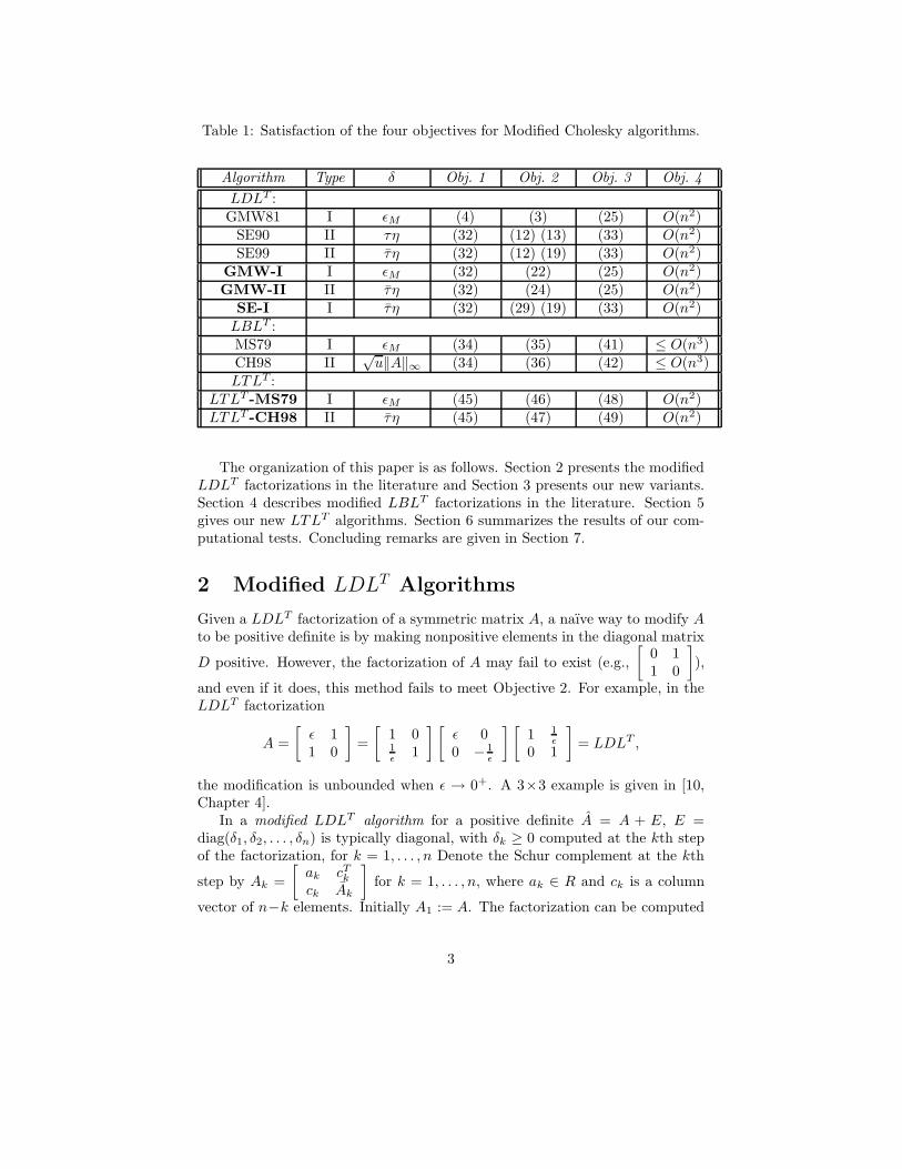
Table 1: Satisfaction of the four objectives for Modified Cholesky algorithms.
Algorithm Type δ Obj. 1 Obj. 2 Obj. 3 Obj. 4
LDLT :GMW81 I εM (4) (3) (25) O(n2)
SE90 II τη (32) (12) (13) (33) O(n2)SE99 II τ η (32) (12) (19) (33) O(n2)
GMW-I I εM (32) (22) (25) O(n2)GMW-II II τ η (32) (24) (25) O(n2)
SE-I I τ η (32) (29) (19) (33) O(n2)LBLT :MS79 I εM (34) (35) (41) ≤ O(n3)CH98 II
√u‖A‖∞ (34) (36) (42) ≤ O(n3)
LTLT :LTLT -MS79 I εM (45) (46) (48) O(n2)LTLT -CH98 II τ η (45) (47) (49) O(n2)
The organization of this paper is as follows. Section 2 presents the modifiedLDLT factorizations in the literature and Section 3 presents our new variants.Section 4 describes modified LBLT factorizations in the literature. Section 5gives our new LTLT algorithms. Section 6 summarizes the results of our com-putational tests. Concluding remarks are given in Section 7.
2 Modified LDLT Algorithms
Given a LDLT factorization of a symmetric matrix A, a naıve way to modify Ato be positive definite is by making nonpositive elements in the diagonal matrix
D positive. However, the factorization of A may fail to exist (e.g.,
[0 11 0
]),
and even if it does, this method fails to meet Objective 2. For example, in theLDLT factorization
A =
[ε 11 0
]=
[1 01ε 1
] [ε 00 − 1
ε
][1 1
ε0 1
]= LDLT ,
the modification is unbounded when ε → 0+. A 3×3 example is given in [10,Chapter 4].
In a modified LDLT algorithm for a positive definite A = A + E, E =diag(δ1, δ2, . . . , δn) is typically diagonal, with δk ≥ 0 computed at the kth stepof the factorization, for k = 1, . . . , n Denote the Schur complement at the kth
step by Ak =
[ak cT
k
ck Ak
]for k = 1, . . . , n, where ak ∈ R and ck is a column
vector of n−k elements. Initially A1 := A. The factorization can be computed
3

Table 2: Notation.
Symbol Description
εM machine epsilonu unit roundoff, εM/2A an n × n symmetric matrixξ maximum magnitude of off-diagonal elements of Aη maximum magnitude of diagonal elements of A
λi(A) ith smallest eigenvalue of Aλmin(A) smallest eigenvalue of Aλmax(A) largest eigenvalue of A
τ 3√
εM
τ 3
√ε2M
by setting
L(k+1:n, k :k) :=ck
ak + δk, D(k, k) := ak + δk and Ak+1 := Ak − ckcT
k
ak + δk(1)
for k = 1, . . . , n − 1. The challenge is to determine δk to satisfy the four ob-jectives. All the algorithms in Sections 2 and 3 follow this model, althoughSchnabel and Eskow [15, 16] originally formulated their algorithm in LLT form.
We may incorporate a diagonal pivoting strategy in our algorithms, sym-metrically interchanging rows and columns at the kth step to ensure that |ak| ≥|Ak(j, j)| (pivoting on the diagonal element of maximum magnitude) or ak ≥Ak(j, j) (pivoting on the element of maximum value) for j = 1, . . . , n−k. Theresulting modified LDLT factorization is in the form
P (A + E)P T = LDLT = LLT , (2)
where P is a permutation matrix.Gill and Murray introduced a stable algorithm in 1974 [9]. It was subse-
quently refined by Gill, Murray, and Wright in 1981 [10, Chapter 4]; we callit GMW81 hereafter. Schnabel and Eskow introduced another modified LDLT
algorithm in 1990 [15]. It was subsequently revised in 1999 [16]. We call thesealgorithms SE90 and SE99, respectively.
2.1 The GMW81 Algorithm
GMW81 determines δk in (1) by setting
ak + δk = max{δ, |ak|,‖ck‖2
∞β2
}
for k = 1, . . . , n, where β > 0 and the small tolerance δ > 0 are preset. We setδ := εM (machine epsilon) as is common in the literature [5, 16].
4
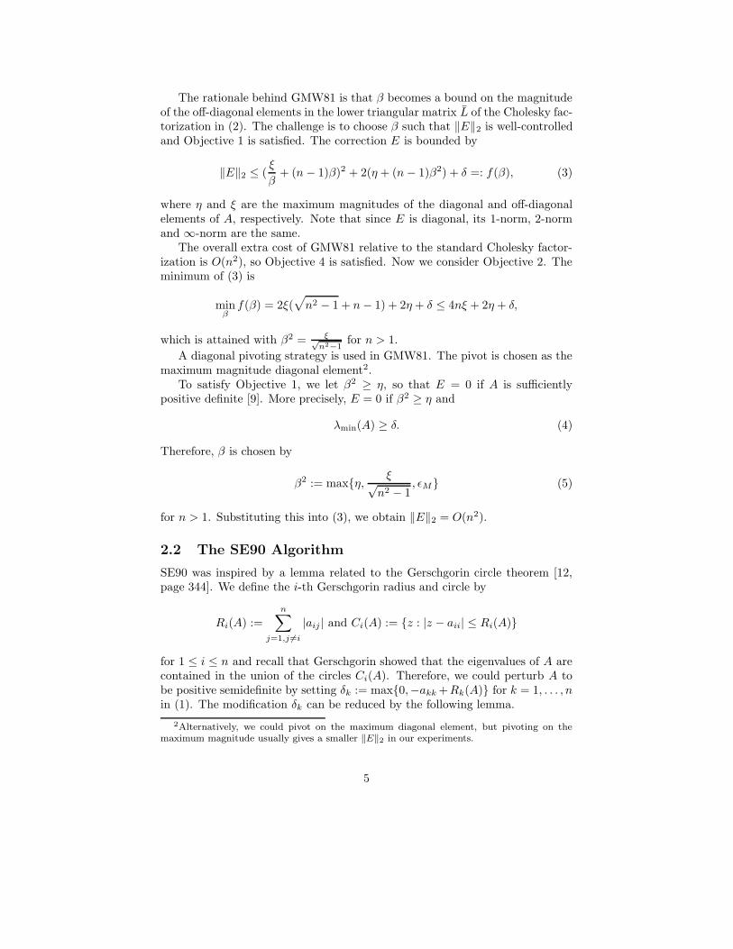
The rationale behind GMW81 is that β becomes a bound on the magnitudeof the off-diagonal elements in the lower triangular matrix L of the Cholesky fac-torization in (2). The challenge is to choose β such that ‖E‖2 is well-controlledand Objective 1 is satisfied. The correction E is bounded by
‖E‖2 ≤ (ξ
β+ (n − 1)β)2 + 2(η + (n − 1)β2) + δ =: f(β), (3)
where η and ξ are the maximum magnitudes of the diagonal and off-diagonalelements of A, respectively. Note that since E is diagonal, its 1-norm, 2-normand ∞-norm are the same.
The overall extra cost of GMW81 relative to the standard Cholesky factor-ization is O(n2), so Objective 4 is satisfied. Now we consider Objective 2. Theminimum of (3) is
minβ
f(β) = 2ξ(√
n2 − 1 + n − 1) + 2η + δ ≤ 4nξ + 2η + δ,
which is attained with β2 = ξ√n2−1
for n > 1.
A diagonal pivoting strategy is used in GMW81. The pivot is chosen as themaximum magnitude diagonal element2.
To satisfy Objective 1, we let β2 ≥ η, so that E = 0 if A is sufficientlypositive definite [9]. More precisely, E = 0 if β2 ≥ η and
λmin(A) ≥ δ. (4)
Therefore, β is chosen by
β2 := max{η,ξ√
n2 − 1, εM} (5)
for n > 1. Substituting this into (3), we obtain ‖E‖2 = O(n2).
2.2 The SE90 Algorithm
SE90 was inspired by a lemma related to the Gerschgorin circle theorem [12,page 344]. We define the i-th Gerschgorin radius and circle by
Ri(A) :=n∑
j=1,j 6=i
|aij | and Ci(A) := {z : |z − aii| ≤ Ri(A)}
for 1 ≤ i ≤ n and recall that Gerschgorin showed that the eigenvalues of A arecontained in the union of the circles Ci(A). Therefore, we could perturb A tobe positive semidefinite by setting δk := max{0,−akk +Rk(A)} for k = 1, . . . , nin (1). The modification δk can be reduced by the following lemma.
2Alternatively, we could pivot on the maximum diagonal element, but pivoting on themaximum magnitude usually gives a smaller ‖E‖2 in our experiments.
5

Lemma 1 Given a symmetric matrix A =
[a cT
c A
]∈ Rn×n, suppose we add
a perturbation δ ≥ {0,−a+‖c‖1} to a, so that a+δ ≥ ‖c‖1. The resulting Schur
complement3 is A := A − ccT
a+δ . Then Ci(A) ⊆ Ci+1(A) for i = 1, . . . , n − 1.
Proof This proof is a condensed version of that in [15]. Let aij and aij denote
the (i, j) entries of A and A respectively for 1 ≤ i, j < n. Also denote c =[(c)1, (c)2, . . . , (c)n−1]
T . For 1 ≤ i < n,
Ri+1(A) − Ri(A) = (Ri+1(A) − Ri(A)) + (Ri(A) − Ri(A)).
The difference between Ri+1(A) and Ri(A) is |(c)i|. In addition, the ith column
of A − A is (c)ica+δ , whose 1-norm minus
(c)2ia+δ is the upper bound for |(Ri(A) −
Ri(A))|. Therefore,
Ri+1(A) − Ri(A) ≥ |(c)i| −|(c)i|(‖c‖1 − |(c)i|)
a + δ
= |(c)i|(1 − ‖c‖1
a + δ) +
(c)2ia + δ
≥ (c)2ia + δ
= aii − aii ≥ 0.
This means that the Gerschgorin circles contract, and the contraction of eachcircle is no less than the perturbation of the circle center. Therefore, Ci(A) ⊆Ci+1(A) for i = 1, . . . , n−1.
Following this result, we can make A + E positive semidefinite by settingδk := max{0,−ak + ‖ck‖1} in (1) for k = 1, . . . , n. Note that ak − ‖ck‖1 is thelower endpoint of the Gerschgorin circle C1(Ak). Repeatedly applying Lemma 1,we obtain δk ≤ max{0,−akk + Rk(A)} for k = 1, . . . , n. Taking the maximumof these values and zero, we define
G := max{0, max{−akk + Rk(A) : k = 1, . . . , n}}.
Then ‖E‖2 ≤ G ≤ η + (n− 1)ξ, where η and ξ are the maximum magnitudes ofthe diagonal and off-diagonal elements of A, respectively. However, this naıvemethod may fail to satisfy Objective 1.
To satisfy Objective 1, SE90 consists of two phases. The 2-phase strategywas also presented in [8]. Phase 1 performs steps of the standard Cholesky fac-torization (i.e., without perturbation, δk := 0), as long as all diagonal elementsof the next Schur complement are sufficiently positive. The pseudo-code is givenin Algorithm 1.
SE90 uses the tolerance δ := τη, where η is the maximum magnitude of thediagonal elements of A, and τ = 3
√εM . Therefore, in Phase 1,
Diag(Ak) ≥ τηIn−k+1 (6)
3Note that the ith row/column of A corresponds to the (i+1)st row/column of A.
6

Algorithm 1 Phase 1 of a 2-Phase Strategy.
{Given a symmetric A ∈ Rn×n and a small tolerance δ > 0.}A1 := A, k := 1Pivot on the maximum diagonal element of A1.
{Denote Ak =
[ak cT
k
ck Ak
], then Diag(Ak) ≤ akIn−k after pivoting.}
if a1 ≥ δ then
while Diag(Ak − ckcTk
ak) ≥ δIn−k and k < n do
Ak+1 := Ak − ckcTk
ak
k := k + 1Pivot on maximum diagonal of Ak.
end whileend if
for k = 1, . . . , min{n, K +1}, where K is the number of steps in Phase 1. IfA is sufficiently positive definite, then K = n and the factorization completeswithout using Phase 2. Otherwise, Phase 1 ends when setting δK+1 := 0 resultsin AK+2 having a diagonal element less than δ. It is not hard to see that
η ≤ η and ξ ≤ ξ + η, (7)
where η and ξ (and η and ξ) are the maximum magnitudes of the diagonal andoff-diagonal elements of AK+1 (and A), respectively [15].
In Phase 2, δk is determined by
δk := max{δk−1,−ak + max{‖ck‖1, τη}} ≤ G + τη, (8)
for k = K+1, . . . , n−2, where G is the maximum of zero and the negative of thelowest Gerschgorin endpoint of AK+1. For the case K = 0, we set δ0 := 0. Therationale for δk ≥ δk−1 is because increasing δk up to δk−1 does not increase‖E‖2 at this point and may possibly reduce the subsequent δi for k < i ≤ n.This nondecreasing strategy can be applied to virtually all modified Choleskyalgorithms with modifications confined to the diagonal.
In experiments, Schnabel and Eskow [15] obtained a smaller value of ‖E‖2
when using special treatment for the final 2×2 Schur complement An−1, setting
δn−1 =δn := max{δn−2,−λ1(An−1)+max{τ(λ2(An−1)−λ1(An−1))
1−τ, τη}} (9)
≤ G +2τ
1 − τ(G + η), (10)
where λ1(An−2) and λ2(An−2) are the smaller and larger eigenvalues of An−2,respectively. The last inequality holds because
−λ1(An−1) ≤ G and λ2(An−1) − λ1(An−1) ≤ 2(G + η).
7

In (9), δn−1 and δn are chosen to obtain the bound
κ2(An−1 + δnI2) ≤1 + (τ/(1 − τ))
τ/(1 − τ)=
1
τ, (11)
where I2 =
[1 00 1
]. Finally, by (8) and (10),
‖E‖2 ≤ G +2τ
1 − τ(G + η). (12)
If K = 0, then G ≤ η + (n − 1)ξ. By (7), if K > 0, then
G ≤ (n − K − 1)(ξ + η). (13)
In either case, ‖E‖2 = O(n). Recall that with GMW81, ‖E‖2 = O(n2).Diagonal pivoting is also used in SE90, as well as the later SE99 algorithm.
The analysis above does not rely on the pivoting, but pivoting reduces ‖E‖2
empirically. In Phase 1, the pivot is chosen as the largest diagonal entry asshown in Algorithm 1.
In Phase 2, one may choose the pivot with the largest lower endpoint of theGerschgorin circle in the current Schur complement. This provides the leastmodification at the current step. In other words, after diagonally interchangingrows and columns, G1(Ak) ≥ Gi(Ak) for k = K+1, . . . , n−2 and i = 1, . . . , n−k+1,where Gi(Ak) = aii −Ri(Ak) is the lower endpoint of the ith Gerschgorin circle
Ci(Ak). However, computing all Gi(Ak) in Phase 2 takes (n−K)3
3 additions andfails to satisfy Objective 4. The proof of Lemma 1 shows
aii − Ri(A) ≥ aii − Ri+1(A) + |(c)i|(1 − ‖c‖1
a + δ)
for i = 1, . . . , n−1. Therefore,
Gi(Ak+1) ≥ Gi+1(Ak) + |(ck)i|(1 − ‖ck‖1
ak + δk)
for k = 1, . . . , n−1 and i = 1, . . . , n−k. Using this fact, we recursively computethe lower bounds of these Gerschgorin intervals by
Gi(Ak+1) := Gi+1(Ak) + |(ck)i|(1 − ‖ck‖1
ak + δk)
for k = 1, . . . , n−1 and i = 1, . . . , n−k. The base cases are Gi(A1) := Gi(A) fori = 1, . . . , n. Computing these estimated lower endpoints Gi(Ak+1) for pivotingtakes 2(n−K)2 additions and 1
2 (n−K)2 multiplications. Hence Objective 4 issatisfied.
8

2.3 The SE99 Algorithm
Although SE90 has a better a priori bound on ‖E‖2 than GMW81, there arematrices for which SE90 gives an inordinately large ‖E‖2. These matrices aregenerally close to being positive definite. The SE99 algorithm [16], was devel-oped to remedy this. In SE99, condition (6) is relaxed into the following twoconditions that possibly increase the number of Phase 1 pivots:
Diag(Ak − ckcTk
ak) ≥ −µηIn−k
for some 0 < µ ≤ 1, and
Diag(Ak) ≥ −µakIn−k+1.
Schnabel and Eskow suggested µ = 0.1 for SE99 [16]. The pseudo-code of therelaxed 2-phase strategy is given in Algorithm 2.
Algorithm 2 Relaxed Phase 1 of a 2-Phase Strategy.
{Given a symmetric A ∈ Rn×n, δ > 0 and 0 < µ ≤ 1.}η := max1≤i≤n |Aii|if Diag(A) ≥ −µηIn then
A1 := A, k := 1Pivot on the maximum diagonal element of A1.
{Denote Ak =
[ak cT
k
ck Ak
], then Diag(Ak) ≤ akIn−k after pivoting.}
while ak ≥ δ and Diag(Ak) ≥ −µakIn−k+1 and Diag(Ak − ckcTk
ak) ≥
−µηIn−k and k < n do
Ak+1 := Ak − ckcTk
ak
k := k + 1Pivot on maximum diagonal of Ak.
end whileend if
In SE99, δ := τ η, where τ = 3
√ε2M , is smaller than τ = 3
√εM in SE90,
potentially keeping ‖E‖ smaller. In Phase 1, there is no perturbation, so δk = 0for k = 1, 2, . . . , K, with K the number of steps in Phase 1. The modificationin Phase 2 turns out to be
δk := max{δk−1,−ak + max{‖ck‖1, τ η}} ≤ G + τ η, (14)
where G is the negative of the lowest Gerschgorin endpoint of AK+1. Recallthat we set δ0 := 0 and δk is nondecreasing, so that δk is nonnegative.
Since small negative numbers are allowed on the diagonal in Phase 1, twochanges have to be made. First, we need to check whether ak ≥ δ at each step,as shown in Algorithm 2, whereas it is not required in Algorithm 1. Second, it
9

is possible that SE99 moves into Phase 2 at the last step (i.e., the number ofsteps in Phase 1 is K = n − 1). In such a case,
δn := max{0,−an + max{ −τ
1 − τan, τη}} ≤ G +
τ
1 − τG + τ η. (15)
Similar to (9) in SE90, the special treatment in SE99 for the final 2×2 Schurcomplement in Phase 2 is
δn−1 =δn := max{δn−2,−λ1(An−1)+max{τ(λ2(An−1)−λ1(An−1))
1−τ, τ η}}
≤ G +2τ
1 − τ(G + η). (16)
By (14), (15) and (16), we obtain
‖E‖2 ≤ G +2τ
1 − τ(G + η). (17)
Although (17) for SE99 looks the same as (12) for SE90, the bound on G in
(17) is different for 0 < K < n. Due to relaxing, the bounds (7) on η and ξ arereplaced by
η ≤ η and ξ ≤ ξ + (1 + µ)η, (18)
where η and ξ (and η and ξ) are the maximum magnitudes of the diagonal andoff-diagonal elements of AK+1 (and A), respectively. Therefore, if 0 < K < n,
G ≤ (n − K − 1)(ξ + (1 + µ)η) + µη. (19)
Recall that K is the number of steps in Phase 1, and SE99 potentially has moresteps staying in Phase 1 than SE90.
The pivoting strategy used in SE99 is the same as that in SE90. Note thatthe bound on ‖E‖2 in (17) for SE99 is independent of the pivoting strategyapplied, and so is (12) for SE90.
3 New Modified LDLT Algorithms
This section presents three variants of the LDLT algorithms, GMW-I, GMW-IIand SE-I, and illustrates their performance.
Experiments used a laptop with an Intel Celeron 2.8GHz CPU using IEEEstandard arithmetic with machine epsilon εM = 2−52 ≈ 2.22 × 10⁻¹⁶. Wemeasure the size of E by the ratios
r2 =‖E‖2
|λmin(A)| and rF =‖E‖F
(∑
λi(A)<0 λi(A)2)1/2. (20)
Note that assuming λmin(A) < 0, the denominators are the norms of the leastmodification to make the matrix positive semidefinite.
10

The random matrices in our experiments are of the form QΛQT , whereQ ∈ Rn×n is a random orthogonal matrix computed by the method of G. W.Stewart [17], and Λ ∈ Rn×n is diagonal with uniformly distributed randomeigenvalues in [−1, 10000], [−1, 1] or [−10000,−1]. For the matrices with eigen-values in [−1, 10000], we impose the condition that there is at least one negativeeigenvalue.
3.1 The GMW-I Algorithm
The GMW81 algorithm, a Type-I algorithm, satisfies ‖E‖2 = O(n2), whereasSE90 and SE99 further guarantee ‖E‖2 = O(n), as shown in (12) and (17),respectively. Schnabel and Eskow [15] pointed out that the 2-phase strategycan drop the bound on ‖E‖2 of GMW81 to be O(n). In our experiments, wenote that incorporating the 2-phase strategy into GMW81 introduces difficultiessimilar to those for SE90, and again relaxing provides the rescue.
We denote by GMW-I the algorithm that uses the Relaxed Phase 1 of SE99with Phase 2 defined by GMW81. Denote the number of steps in Phase 1 byK. Then δk = 0 for k = 1, 2, . . . , K. Instead of (3), the bound on ‖E‖2 is
‖E‖2 ≤ (ξ
β+ (n − K − 1)β)2 + 2(η + (n − K − 1)β2) + δ, (21)
where η and ξ are the maximum magnitudes of the diagonal and off-diagonal ele-ments of AK+1, respectively. Now we do not need β2 ≥ η to satisfy Objective 1,so β is chosen as the minimizer of (21),
β2 = max{ ξ√(n − K)2 − 1
, εM}
for n − K > 1. Substituting this into (21) and invoking (18), we obtain
‖E‖2 ≤ 4(n − K)ξ + 2η + δ ≤ 4(n − K)(ξ + (1 + µ)η) + 2η + δ = O(n), (22)
where we ignore the extreme case β2 = εM .We still use δ := εM as in GMW81 and set µ = 0.75 in the relaxed 2-phase
strategy since it is an empirically good value for the GMW algorithms. (Recallthat µ = 0.1 for SE99.) Pivoting reduces ‖E‖2 in the original GMW81 algo-rithm; we pivot on the maximum element instead of the maximum magnitudeelement in Phase 2, because on average the resulting κ2(A + E) is smaller inour experiments. We call our variant GMW-I.
Figure 1 shows our experimental result. The GMW-I algorithm performedwell, but for the random matrices with eigenvalues in [−10000,−1], the ‖E‖2
was a few times larger than in the original GMW81. Nevertheless, in practi-cal optimization problems, negative definite Hessian matrices rarely occur, andindefinite Hessian matrices are usually close to being positive definite. The non-decreasing strategy was also tried. For the random matrices with eigenvaluesin [−1, 1] and [−10000,−1], the nondecreasing strategy substantially reducedκ2(A + E) but roughly doubled ‖E‖F (though with ‖E‖2 comparable). Notethat the bound on ‖E‖2 in (3) is preserved with the nondecreasing strategy.
11

1
10
100
1000
10000
100000
0 5 10 15 20 25 30
r F
matrix
(a) n=100, eig. range [-1,10000]
1 10
100 1000
10000 100000 1e+06 1e+07
0 5 10 15 20 25 30
κ 2(A
+E
)
matrix
(b) n=100, eig. range [-1,10000]
1
10
100
1000
0 5 10 15 20 25 30
r F
matrix
(c) n=100, eig. range [-1,1]
1 10
100 1000
10000 100000 1e+06 1e+07 1e+08 1e+09 1e+10
0 5 10 15 20 25 30
κ 2(A
+E
)
matrix
(d) n=100, eig. range [-1,1]
1
10
100
0 5 10 15 20 25 30
r F
matrix
(e) n=100, eig. range [-10000,-1]
1
10
100
0 5 10 15 20 25 30
κ 2(A
+E
)
matrix
(f) n=100, eig. range [-10000,-1]
Figure 1: Measures of rF and κ2(A + E) for the Type-I GMW algorithms for30 random matrices with n = 100. Key: original GMW81 —, with 2-phasestrategy + , with relaxed 2-phase strategy (GMW-I) × , with relaxed 2-phaseand nondecreasing strategy 2 .
12

3.2 The GMW-II Algorithm
In this subsection we introduce our GMW-II algorithm, a Type-II variant of the(Type-I) GMW81 algorithm. We apply the nondecreasing strategy and chooseδk in (1) to be
ak + δk := max{δ, ak + δk−1,‖ck‖2
∞β2
}
for k = 1, . . . , n, where β > 0 and small tolerance δ > 0 are preset, and δ0 := 0.The magnitude of the off-diagonal elements in L is still bounded by β, whereLDLT = LLT .
The bound on ‖E‖2 for GMW81 is given in (3). For the Type-II GMWalgorithm, it is
‖E‖2 ≤ (ξ
β+ (n − 1)β)2 + (η + (n − 1)β2) + δ =: f(β). (23)
Equality is attained with β2 = ξ√n2−n
for n > 1. Recall that η and ξ are the
maximum magnitudes of the diagonal and off-diagonal elements of A, respec-tively. The minimum of (23) is
minβ
f(β) = 2ξ(√
n2 − n + n − 1) + η + δ ≤ 4nξ + η + δ.
The minimum is attained with β2 = ξ√n2−n
for n > 1. Therefore, β is chosen
by
β2 := max{η,ξ√
n2 − n, εM}
for n > 1, where β2 ≥ η is for satisfying Objective 1 with pivoting. Substitutingthis into (23), we obtain ‖E‖2 = O(n2).
The relaxed 2-phase strategy in Algorithm 2 is also incorporated into ourGMW-II algorithm. Therefore, the bound on ‖E‖2 is
‖E‖2 ≤ (ξ
β+ (n − K − 1)β)2 + (η + (n − K − 1)β2) + δ, (24)
where K is the number of steps in Phase 1, and η and ξ are the maximummagnitudes of the diagonal and off-diagonal elements of AK+1, respectively.Since β2 ≥ η is not required for satisfying Objective 1, β is determined by
β2 := max
{ξ√
(n − K)2 − (n − K), εM
}
for n − K > 1. Substituting this into (24), we obtain
‖E‖2 ≤ 4(n − K)ξ + η + δ ≤ 4(n − K)(ξ + (1 + µ)η) + η + δ = O(n),
where we ignore the extreme case β2 = εM . The last inequality is derived using(18).
13

The diagonal pivoting strategy can be incorporated into the Type-II GMWalgorithms. We pivot on the maximum element for our GMW-II algorithm, asin the GMW-I algorithm. Note that all the a priori bounds on ‖E‖2 given abovefor all algorithms in the GMW class are independent of the pivoting strategyapplied, if any.
1
10
100
1000
10000
100000
0 5 10 15 20 25 30
r F
matrix
(a) n=100, eig. range [-1,10000]
1 10
100 1000
10000 100000 1e+06 1e+07 1e+08
0 5 10 15 20 25 30
κ 2(A
+E
)
matrix
(b) n=100, eig. range [-1,10000]
1
10
100
1000
0 5 10 15 20 25 30
r F
matrix
(c) n=100, eig. range [-1,1]
1 10
100 1000
10000 100000 1e+06 1e+07
0 5 10 15 20 25 30κ 2
(A+
E)
matrix
(d) n=100, eig. range [-1,1]
1
10
100
1000
0 5 10 15 20 25 30
r F
matrix
(e) n=100, eig. range [-10000,-1]
1 10
100 1000
10000 100000 1e+06 1e+07 1e+08
0 5 10 15 20 25 30
κ 2(A
+E
)
matrix
(f) n=100, eig. range [-10000,-1]
Figure 2: Measures of rF and κ2(A+E) for the Type-II GMW algorithms for 30random matrices with n = 100, nondecreasing strategy invoked. Key: originalType-II GMW —, with 2-phase strategy 2 , with relaxed 2-phase strategy(GMW-II) × .
Recall that GMW81 and GMW-I use δ := εM . For the Type-II GMW al-gorithms, we use δ := 3
√ε2Mη as in SE99. Our experimental results are shown
in Figure 2. Similar to SE90 and the Type-I GMW algorithms, incorporat-ing the 2-phase strategy results in difficulties for the matrices with eigenvalues[−1, 10000], and relaxing is the cure.
14
For all algorithms in the GMW class, the worst-case condition number is
κ2(A + E) = O(n3(ξ + η
δ)n). (25)
The proof uses Theorem 1, Lemma 3, the bounds [δ, η + (n − 1)β2] for thediagonal elements in D, and the bound β for the magnitude of the off-diagonalelements in L, where P (A + E)P T = LDLT = LLT as denoted in (2).
Whether the 2-phase strategy or the relaxed 2-phase strategy is applied, thebound on κ2(A + E) remains exponential using (7) and (18), respectively. Thebounds are not changed when the nondecreasing strategy is applied. All themodified Cholesky algorithms in Sections 2 and 3 are numerically stable, sincethey can be regarded as the Cholesky factorizations of the symmetric positivedefinite matrix A + E [5].
3.3 The SE-I Algorithm
Both SE90 and SE99 are Type-II algorithms. In this section we present theType-I variant corresponding to SE99, denoted by SE-I, by making three changes.First, instead of (14), we determine δk by
δk := max{0,−2ak,−ak + max{‖ak‖1, τη}} ≤ max{2G, G + τ η} (26)
for k = K +1, . . . , n−2. Second, instead of (16), the special treatment of thelast 2×2 Schur complement in Phase 2 to keep ‖E‖2 small is
δn−1 =δn := max{0,−2λ1(An−1),−λ1(An−1)+max{τ(λ2(An−1)−λ1(An−1))
1 − τ, τ η}}
≤ max{2G, G +2τ
1 − τ(G + η)}. (27)
Note that κ2(An−1 + δnI2) ≤ min{κ2(An−1),1τ }. The derivation is similar to
that of (10). Third, if the algorithm switches to Phase 2 at the last step, thenδn is determined by
δn = max{0,−2an,−an + max{ −τ
1− τan, τ η}}
≤ max{2G, G +τ
1 − τ(G + η)} (28)
instead of (15).By (26), (27) and (28), we obtain
‖E‖2 ≤ max{2G, G +2τ
1 − τ(G + η)}. (29)
Comparing (29) with (17), the bound on ‖E‖2 for SE-I is less than twice as thatfor SE99.
Now we investigate the satisfaction of Objective 1 for the GMW and SEalgorithms. We begin with a theorem of Ostrowski [12, page 224].
15

Theorem 1 (Ostrowski) Suppose we are given a symmetric M ∈ Cn×n anda nonsingular S ∈ Cn×n. There exists θk > 0 such that
λk(SMS∗) = θkλk(M),
where λ1(SS∗) ≤ θk ≤ λn(SS∗).
Consider the 2-phase strategy presented in Algorithm 1 and the relaxed 2-phase strategy presented in Algorithm 2 with pivoting on the maximum diagonalelement. Clearly E = 0 if the factorization is done in Phase 1. The derivation ofthe condition under which the algorithm runs to completion without switchingto Phase 2 is by finite induction. We denote the incomplete LDLT factorizationof a symmetric matrix A ∈ Rn×n after step k by LkDkLT
k , where
Dk =k n−k
kn−k
[Dk 00 Sk
],
with Dk diagonal and Sk the Schur complement. We claim that the followingcondition guarantees E = 0:
λmin(A) ≥ δ‖LkLTk ‖2 (30)
for k = 1, . . . , n−1. At the beginning of step k, we assume that the diagonal ele-ments of the Schur complement are all larger than or equal to δ, and investigatewhether this condition holds in the next Schur complement4. By Theorem 1and (30),
λmin(Dk)λmax(LkLTk ) ≥ λmin(A) ≥ δ‖LkL
Tk ‖2 = δλmax(LkLT
k ),
and therefore λmin(Dk) ≥ δ, so
λmin(Sk) ≥ λmin(Dk) ≥ δ,
which implies Diag(Sk) ≥ δIn−k. By induction, we stay in Phase 1 during thewhole factorization. We conclude that if (30) holds, then E = 0.
In the next two lemmas we develop bounds on ‖LLT‖2 and on λmin(LLT ),in order to bound the condition number of A + E for algorithms in Sections 4and 5.
Lemma 2 If the positive semidefinite Hermitian matrix M ∈ Cn×n has a di-agonal element equal to 1, (i.e., mkk = 1 for some 1 ≤ k ≤ n), then
λmin(M) ≤ 1 ≤ λmax(M).
4For the base case, we have λmin(A) ≥ δ from (30), so A − δI is positive definite andtherefore diag(A) ≥ δI.
16

Proof Let M = UΛU∗ denote the spectral decomposition of M , and a := U ∗ek.Since mkk = 1,
1 = eTk Mek = a∗U∗(UΛU∗)Ua = a∗Λa.
Note that a∗a = 1. We conclude that the weighted average of the eigenvaluesof M is 1. Therefore, λmin(M) ≤ 1 ≤ λmax(M).
Lemma 3 5 For any lower unit triangular matrix L ∈ Rn×n with |(L)ij | ≤ γfor 1 ≤ j < i ≤ n,
1 ≤ λmax(LLT ) ≤ n +1
2n(n − 1)γ2,
and(1 + γ)2−2n ≤ λmin(LLT ) ≤ 1.
Proof By Lemma 2, λmin(LLT ) ≤ 1 ≤ λmax(LLT ). Next, an upper bound onλmax(LLT ) is λmax(LLT ) ≤ trace(LLT ) ≤ n + 1
2n(n − 1)γ2. Computing theinverse of a lower triangular matrix, we obtain (L−1)ii = 1 for i = 1, . . . , n and
the bounds |(L−1)ij | ≤ γ∑i
k=j+1 |(L−1)ik | for 1 ≤ j < i ≤ n. The solution tothis recursion is
|(L−1)ij | ≤ γ(1 + γ)i−j−1
for 1 ≤ j < i ≤ n. Therefore,
λmin(LLT )−1 = ‖(LLT )−1‖2 ≤ ‖L−1‖22 ≤ ‖L−1‖1‖L−1‖∞ ≤ (1 + γ)2n−2.
Now we can bound ‖LkLTk ‖2 in (30). Pivoting on the maximum diagonal
element of each Schur complement, the magnitude of the elements in Lk arebounded by 1 for all k. By Lemma 3,
‖LkLTk ‖2 ≤ 1
2n(n + 1). (31)
Substituting this into (30), we obtain the following result. For algorithms GMW-I, GMW-II, SE90, SE99, and SE-I that use the 2-phase strategy or the relaxed2-phase strategy, if
λmin(A) ≥ 1
2n(n + 1)δ, (32)
then by (30) and (31) we conclude that E = 0.Our experimental results are shown in Figure 3. For the random matrices
with eigenvalues in [−1, 10000], SE-I resulted in larger ‖E‖2 and ‖E‖F butsubstantially smaller κ2(A + E) than those of SE99. For the random matriceswith eigenvalues in [−1, 1] and [−10000,−1], SE-I had comparable ‖E‖2, smaller‖E‖F , but larger κ2(A + E) than SE99.
5Cheng and Higham [5] presented this lemma with γ = 7+√
17
4≈ 2.781.
17

1
10
100
0 5 10 15 20 25 30
r F
matrix
(a) n=100, eig. range [-1,10000]
1
100
10000
1e+06
1e+08
1e+10
1e+12
0 5 10 15 20 25 30
κ 2(A
+E
)
matrix
(b) n=100, eig. range [-1,10000]
1
10
0 5 10 15 20 25 30
r F
matrix
(c) n=100, eig. range [-1,1]
1
10
100
0 5 10 15 20 25 30
κ 2(A
+E
)
matrix
(d) n=100, eig. range [-1,1]
1
10
0 5 10 15 20 25 30
r F
matrix
(e) n=100, eig. range [-10000,-1]
1
10
0 5 10 15 20 25 30
κ 2(A
+E
)
matrix
(f) n=100, eig. range [-10000,-1]
Figure 3: Measures of rF and κ2(A + E) for the SE algorithms for 30 randommatrices with n = 100. Key: original SE99 —, Type-I SE99 (SE-I) 2 , Type-ISE99 with nondecreasing strategy × .
18

The nondecreasing strategy can be incorporated into the Type-I SE algo-rithm. The resulting ‖E‖2, ‖E‖F and κ2(A + E) were comparable to thoseof SE-I for the random matrices with eigenvalues in [−1, 10000], and compara-ble to those of SE99 for the random matrices with eigenvalues in [−1, 1] and[−10000,−1]. Incorporating the non-relaxed 2-phase strategy into the Type-ISE algorithms is possible, but it would result in difficulties similar to those ofSE90.
For all the algorithms in the SE class, the worst-case condition number is
κ2(A + E) = O((ξ + η)n34n
δ). (33)
The sketch of the proof is similar to that for the GMW algorithms. In practice,the condition number is bounded by about 1/τ and 1/τ respectively for SE90and SE99 [15], and is comparable to κ2(A) for SE-I.
4 Modified LBLT Algorithms
Any symmetric matrix A ∈ Rn×n has an LBLT factorization, where B is blockdiagonal with block order 1 or 2 [2, 3, 4]. A modified LBLT algorithm firstcomputes the LBLT factorization, and then perturbs B = B+∆B to be positivedefinite, so that P (A + E)P T = LBLT is positive definite as well, where P isthe permutation matrix for pivoting.
More and Sorensen suggested a modified LBLT algorithm [13] which we call
MS79. Each 1×1 block in B, denoted by d, is modified to be d := max{δ, |d|},with δ > 0 the preset small tolerance. For each 2×2 block D, its spectral
decomposition D = U
[λ1
λ2
]UT is modified to be D := U
[λ1
λ2
]UT ,
where λi := max{δ, |λi|} for i = 1, 2.Cheng and Higham proposed another modified LBLT algorithm [5] which
we call CH98. Each 1×1 block d is modified to be d := max{δ, d}, with δ > 0the preset small tolerance. Each 2×2 block D, with its spectral decomposition
denoted by D = U
[λ1
λ2
]UT , is modified to be D := U
[λ1
λ2
]UT ,
where λi = max{δ, λi} for i = 1, 2.The key distinction is that MS79 is a Type-I algorithm, whereas CH98 is
of Type II. The MS79 algorithm was developed before the fast Bunch-Parlettand bounded Bunch-Kaufman pivoting strategies (rook pivoting) for the LBLT
factorization [2], but rook pivoting is also applicable to MS79. For MS79, weset δ := εM . Cheng and Higham [5] suggested δ :=
√u‖A‖∞ for CH98, where
u = εM/2 is the unit roundoff.MS79 predated the four objectives. Cheng and Higham investigated the
objectives for CH98 [5], and our analysis for MS79 is similar.For both MS79 and CH98, if λmin(B) ≥ δ, then E = 0. By Theorem 1, if A
19

is positive definite, λmin(B) ≥ λmin(A)λmax(LLT ) . Therefore, E = 0 is guaranteed when
λmin(A) ≥ δ‖LLT‖2. (34)
Consider ‖E‖2 for MS79. By Theorem 1,
‖E‖2 = λmax(E) = λmax(L∆BLT ) ≤ λmax(LLT )λmax(∆B)
= λmax(LLT ) max{δ − λmin(B),−2λmin(B), 0}.
By Theorem 1 again, −λmin(B) ≤ − λmin(A)λmin(LLT ) and −λmin(B) ≥ − λmin(A)
λmax(LLT ) for
λmin(A) < 0. Therefore,
‖E‖2 ≤ −2λmin(A)κ2(LLT ) for λmin(A) ≤ −δ‖LLT‖2. (35)
Similarly, the bound on ‖E‖2 for CH98 is
‖E‖2 ≤ δ‖LLT‖2 − λmin(A)κ2(LLT ) for λmin(A) ≤ 0. (36)
Now we assess how well Objective 3 is satisfied for MS79. By Theorem 1,
λmin(A + E) ≥ λmin(LLT )λmin(B)
= λmin(LLT ) max{δ, min1≤i≤n
|λi(B)|} (37)
≥ λmin(LLT ) max{δ, min1≤i≤n |λi(A)|λmax(LLT )
}, (38)
and
λmax(A + E) ≤ λmax(LLT )λmax(B)
= λmax(LLT ) max{δ,−λmin(B), λmax(B)} (39)
≤ λmax(LLT ) max{δ, −λmin(A)
λmin(LLT ),
λmax(A)
λmin(LLT )}. (40)
By (37) and (39),κ2(A + E) ≤ κ2(LLT )κ2(B).
By (38) and (40),κ2(A + E) ≤ κ2(LLT )2κ2(A). (41)
The bound on κ2(A + E) for CH98 [5] is
κ2(A + E) ≤ κ2(LLT ) max{1,λmax(A)
λmin(LLT )δ}. (42)
There are four pivoting algorithms for the LBLT factorization: Bunch-Parlett (complete pivoting) [4], Bunch-Kaufman (partial pivoting) [3], fast Bunch-Parlett and bounded Bunch-Kaufman (rook pivoting) [2], denoted by BP, BK,FBP and BBK, respectively. All these algorithms have a preset argument
20

0 < α < 1. The BK algorithm takes O(n2) time for pivoting, but the ele-ments in L are unbounded. It is discouraged for the modified LBLT algorithmsbecause Objectives 1–3 may not be satisfied. For example, the following LBLT
factorization [11] is produced with the BK pivoting strategy for ε 6= 0,
A =
0 ε 0ε 0 10 1 1
=
10 11/ε 0 1
0 εε 0
1
1 0 1/ε
1 01
= LBLT .
Applying MS79 or CH98 and assuming 0 < ε ≤ δ, we obtain
E =
10 11/ε 0 1
δ −ε−ε δ
1
1 0 1/ε1 0
1
=
δ −ε δ/ε−ε δ −1δ/ε −1 1+δ
.
When ε → 0+, ‖E‖ → ∞, so Objective 2 is not satisfied.From (34)–(42), it is clear that λmin(LLT ), λmax(LLT ) and κ2(LLT ) play an
important role for the satisfaction of Objectives 1–3 for both MS79 and CH98.The BP, BBK and FBP algorithms all produce a bound on the elements in
L in terms of the pivoting argument α, suggested to be α = 1+√
178 ≈ 0.640
to minimize the bound on the element growth of the Schur complements [2, 3,4]. The corresponding element bound of the unit lower triangular matrix L is
γ = 7+√
174 ≈ 2.781. Alternatively, we could choose α = 0.5 to minimize the
element bound of L [6, Table 3.1], which is γ = 2, leading to sharper boundson λmin(LLT ), λmax(LLT ) and κ2(LLT ). The bounds in Table 3 are obtainedusing Lemma 3.
Table 3: Bounds for the LBLT factorization with the BP, BBK or FBP pivotingalgorithm.
α γ λmin(LLT ) λmax(LLT ) κ2(LLT )1+
√17
87+
√17
4 ≥ 3.7812−2n ≤ 4n2 − 3n ≤ (4n2 − 3n)3.7812n−2
0.5 2 ≥ 32−2n ≤ 2n2 − n ≤ (2n2 − n)32n−2
Although α = 12 results in smaller bounds, α = 1+
√17
8 ≈ 0.640 is a betterchoice in practice, as shown in Figure 4.
The BP pivoting strategy takes 16n3 + O(n2) comparisons and does not
meet Objective 4. The number of comparisons for the BBK and FBP pivotingstrategies are between those of the BK and BP algorithms (i.e., between O(n2)and O(n3)). There are matrices that require traversing the whole matrix ofeach Schur complement with either the BBK or the FBP pivoting strategy [2].Hence they take Θ(n3) comparisons for pivoting in worst cases and fail to meetObjective 4.
Here and throughout the remainder of this paper, we assume the pivotingstrategy applied to the MS79 and CH98 is BBK, unless otherwise noted.
21

1
10
100
1000
10000
0 5 10 15 20 25 30
r 2
matrix
(a) n=100, eig. range [-1,10000]
1
100
10000
1e+06
1e+08
1e+10
1e+12
0 5 10 15 20 25 30
κ 2(A
+E
)
matrix
(b) n=100, eig. range [-1,10000]
1
10
100
0 5 10 15 20 25 30
r 2
matrix
(c) n=100, eig. range [-1,1]
1
100
10000
1e+06
1e+08
1e+10
1e+12
0 5 10 15 20 25 30
κ 2(A
+E
)
matrix
(d) n=100, eig. range [-1,1]
0
0.5
1
1.5
2
2.5
0 5 10 15 20 25 30
r 2
matrix
(e) n=100, eig. range [-10000,-1]
1
10
100
1000
10000
0 5 10 15 20 25 30
κ 2(A
+E
)
matrix
(f) n=100, eig. range [-10000,-1]
Figure 4: Measures of r2 and κ2(A + E) for MS79 and CH98 for 30 randommatrices with n = 100. Key: MS79 α = 0.640 —, MS79 α = 0.5 + , CH98α = 0.640 × , CH98 α = 0.5 2 .
22

Three remarks are in order. First, both MS79 and CH98 satisfy Objectives 1–3. Second, the bound on ‖E‖2 for MS79 is about twice that for CH98, whereasA + E is generally better conditioned for MS79 than for CH98. Third, bothalgorithms fail to satisfy Objective 4 in the worst case.
5 A New Approach via Modified LTLT Factor-
ization
Aasen [1], Parlett and Reid [14] introduced the LTLT factorization and itsapplication to solving symmetric linear systems. We denote the factorizationby PAP T = LTLT , where T is symmetric tridiagonal, and L is unit lowertriangular with the magnitude of its elements bounded by 1 and the off-diagonalelements in the first column all zero.
The work in computing Aasen’s LTLT factorization is about the same asthat of the Cholesky factorization, whereas the formulation by Parlett and Reiddoubles the cost. In both formulations the storage is the same as that requiredby the Cholesky factorization, and the numerical stability of its use in solvinglinear systems is empirically comparable to that of the LBLT factorization [2].
Our new approach arises from the fact that A is positive definite if and only ifT is positive definite. A modified LTLT algorithm makes T = T+∆T symmetricpositive definite, and the resulting factorization A = P (A + E)P T = LTLT isalso symmetric positive definite.
We can apply the modified LDLT algorithms in Sections 2 and 3 and themodified LBLT algorithms in Section 4 to the matrix T . The resulting mod-ified LTLT factorization roughly satisfies Objective 1, assuming the modifiedCholesky algorithm applied to T satisfies Objective 1. Our method was inspiredby the merits of triadic structure (no more than two off-diagonal elements inevery column of a matrix) discussed in [6].
The triadic structure of a symmetric matrix is preserved in the LDLT orLBLT factorizations [6, Theorem 2.5]. This implies that the modified LDLT
or LBLT algorithms in Sections 2–4 applied to a symmetric triadic matrix arevery efficient. Recall that both MS79 and CH98 have difficulties in satisfyingObjective 4. The potential excessive cost can be reduced to be O(n2) by insteadapplying MS79 or CH98 to the symmetric tridiagonal matrix T of the LTLT
factorization. We call the resulting algorithms LTLT -MS79 and LTLT -CH98,respectively. For LTLT -MS79, we use δ := εM . For LTLT -CH98, we useδ := 3
√ε2Mη, as used in SE99.
Table 4 compares the costs of these LBLT pivoting strategies for symmetricand symmetric tridiagonal matrices. We use the BBK pivoting strategy for bothMS79 and CH98, because it is the cheapest pivoting strategy that guarantees abounded L. Even so, Objective 4 is not satisfied in worst cases. We use the BPpivoting strategy for both LTLT -CH98 and LTLT -MS79. Then Objective 4 issatisfied [6], even though BP is the most expensive pivoting strategy.
Given a symmetric matrix A ∈ Rn×n, we denote its LTLT factorization
23

Table 4: Comparison costs of various pivoting strategies for the LBLT factor-ization.
Symmetric Matrix General Tridiagonalcase worst best worst bestBP O(n3) O(n2)FBP O(n3) O(n2) O(n2) O(n)BBK O(n3) O(n2) O(n2) O(n)
by PAP T = LTLT , and the LBLT factorization of T by P T P T = LBLT .The resulting sandwiched factorization is PAP T = LP T LBLT PLT . Adding aperturbation ∆B to B to make it positive definite, the modified factorizationof T is P (T + ∆T )P T = L(B + ∆B)LT . The modified LTLT factorization is
P (A + E)P T = LP T L(B + ∆B)LT PLT . (43)
The matrix L is unit lower triangular with the magnitude of all elements boundedby 1 and all the off-diagonal elements in the first column zero. By Lemma 3,the LTLT factorization satisfies
λmax(LLT ) ≤ 12n(n − 1)
λmin(LLT ) ≥ 24−2n (44)
for n > 1. Lemma 4 gives the bounds on λmax(LLT ) and λmin(LLT ), where Lis triadic and unit lower triangular.
Lemma 4 Let Fγ(k) =∑dk/2e
i=1
(k−ii−1
)γk−i and Φγ =
1+√
1+4/γ
2 γ for k ∈ N and
γ > 0. For any triadic and unit lower triangular L ∈ Rn×n with the magnitudeof the off-diagonal elements bounded by γ,
1. 11+(1/γ)Φ
k−1γ ≤ Fγ(k) ≤ Φk−1
γ for k ∈ N .
2. (L−1)ij ≤ Fγ(i−j+1) for 1 ≤ j ≤ i ≤ n.
3. λmax(LLT ) ≤ n + (2n − 3)γ2 for n > 1.
4. λmin(LLT ) ≥ (Φγ−1Φn
γ−1 )2.
Proof Part one of this lemma is [6, Lemma 5.4]. Part two is from the proof of[6, Lemma 5.6]. For part three,
λmax(LLT ) ≤ trace(LLT ) = ‖L‖2F ≤ n + (2n − 3)γ2,
for n > 1. Finally, by parts one and two,
λmin(LLT )−1 = ‖(LLT )−1‖2 = ‖L−1‖22 ≤ ‖L−1‖1‖L−1‖∞
≤ (
n∑
k=1
Fγ(k))2 ≤ (
n∑
k=1
Φk−1γ )2 = (
Φnγ − 1
Φγ − 1)2.
24

Now we can assess the satisfaction of Objectives 1–3 for our LTLT -MS79and LTLT -CH98 algorithms. To ensure a bounded L of the LBLT factorization,we can use BP, FBP or BBK, but not BK. By (34), λmin(T ) ≥ δ‖LLT ‖2 impliesE = 0. By Theorem 1, if A is positive definite, λmin(A) ≥ λmin(T )λmin(LLT ).We conclude that E = 0 if
λmin(A) ≥ δ‖LLT ‖2λmin(LLT ). (45)
For LTLT -MS79, by Theorem 1 and (35),
‖E‖2 = λmax(E) = λmax(L∆TLT )
≤ λmax(LLT )λmax(∆T ) = ‖LLT‖2‖∆T‖2
≤ −2λmin(A)κ2(LLT )κ2(LLT ) (46)
for λmin(A) ≤ −δ‖LLT‖2‖LLT ‖2. For LTLT -CH98, by Theorem 1 and (36),
‖E‖2 ≤ δ‖LLT‖2‖LLT ‖2 − λmin(A)κ2(LLT )κ2(LLT ) (47)
for λmin(A) ≤ 0. For LTLT -MS79, by Theorem 1 and (41),
κ2(A + E) ≤ κ2(LLT )κ2(T + ∆T )
≤ κ2(LLT )κ2(LLT )2κ2(T )
≤ κ2(LLT )2κ2(LLT )2κ2(A). (48)
For LTLT -CH98, by Theorem 1 and (42),
κ2(A + E) ≤ κ2(LLT )κ2(LLT ) max{1,λmax(T )
λmin(LLT )δ}
≤ κ2(LLT )κ2(LLT ) max{1,λmax(A)
λmin(LLT )λmin(LLT )δ}. (49)
Note that the pivoting argument used in P T P T = LBLT is α =√
5−12 ≈
0.618 for symmetric triadic matrices [6, Theorem 4.1]. The corresponding ele-
ment bound of L is γ =√
5+32 ≈ 2.618. One may choose α = 0.5 to obtain the
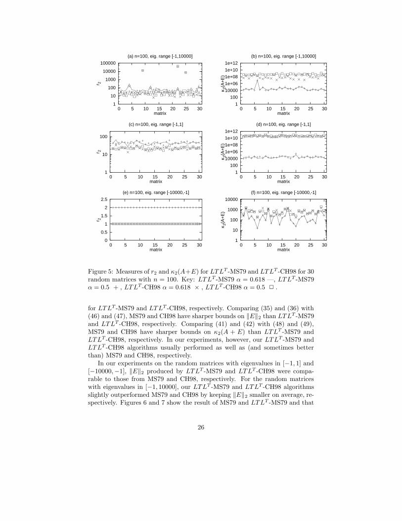
minimum element bound of L [6, Table 3.1], which is γ = 2, but it could resultin an excessive ‖E‖2 for random matrices with eigenvalues [−1, 10000] as shownin Figure 5.
The bounds on ‖LLT‖2 and λmin(LLT ) are given in (44). The bounds on
‖LLT ‖2 and λmin(LLT ) are in Lemma 4 with γ =√
5+32 ≈ 2.618. We conclude
that‖LLT‖2‖LLT ‖2 ≤ 7.5n3 − 17.5n2 + 10.5n
λmin(LLT )λmin(LLT ) ≥ 914n(3.4n−1)2
(50)
for n > 1.Comparing (50) with Table 3 with α = 1+
√17
8 , ‖LLT‖2 and λmin(LLT ) for
MS79 and CH98 have sharper bounds than ‖LLT‖2‖LLT ‖2 and λmin(LLT )λmin(LLT )
25
1
10
100
1000
10000
100000
0 5 10 15 20 25 30
r 2
matrix
(a) n=100, eig. range [-1,10000]
1
100
10000
1e+06
1e+08
1e+10
1e+12
0 5 10 15 20 25 30
κ 2(A
+E
)
matrix
(b) n=100, eig. range [-1,10000]
1
10
100
0 5 10 15 20 25 30
r 2
matrix
(c) n=100, eig. range [-1,1]
1
100
10000
1e+06
1e+08
1e+10
1e+12
0 5 10 15 20 25 30
κ 2(A
+E
)
matrix
(d) n=100, eig. range [-1,1]
0
0.5
1
1.5
2
2.5
0 5 10 15 20 25 30
r 2
matrix
(e) n=100, eig. range [-10000,-1]
1
10
100
1000
10000
0 5 10 15 20 25 30
κ 2(A
+E
)
matrix
(f) n=100, eig. range [-10000,-1]
Figure 5: Measures of r2 and κ2(A+E) for LTLT -MS79 and LTLT -CH98 for 30random matrices with n = 100. Key: LTLT -MS79 α = 0.618 —, LTLT -MS79α = 0.5 + , LTLT -CH98 α = 0.618 × , LTLT -CH98 α = 0.5 2 .
for LTLT -MS79 and LTLT -CH98, respectively. Comparing (35) and (36) with(46) and (47), MS79 and CH98 have sharper bounds on ‖E‖2 than LTLT -MS79and LTLT -CH98, respectively. Comparing (41) and (42) with (48) and (49),MS79 and CH98 have sharper bounds on κ2(A + E) than LTLT -MS79 andLTLT -CH98, respectively. In our experiments, however, our LTLT -MS79 andLTLT -CH98 algorithms usually performed as well as (and sometimes betterthan) MS79 and CH98, respectively.
In our experiments on the random matrices with eigenvalues in [−1, 1] and[−10000,−1], ‖E‖2 produced by LTLT -MS79 and LTLT -CH98 were compa-rable to those from MS79 and CH98, respectively. For the random matriceswith eigenvalues in [−1, 10000], our LTLT -MS79 and LTLT -CH98 algorithmsslightly outperformed MS79 and CH98 by keeping ‖E‖2 smaller on average, re-spectively. Figures 6 and 7 show the result of MS79 and LTLT -MS79 and that
26
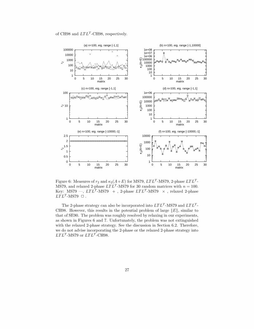
of CH98 and LTLT -CH98, respectively.
1
10
100
1000
10000
100000
0 5 10 15 20 25 30
r 2
matrix
(a) n=100, eig. range [-1,1]
1 10
100 1000
10000 100000 1e+06 1e+07 1e+08
0 5 10 15 20 25 30
κ 2(A
+E
)
matrix
(b) n=100, eig. range [-1,10000]
1
10
100
0 5 10 15 20 25 30
r 2
matrix
(c) n=100, eig. range [-1,1]
1
10
100
1000
10000
100000
1e+06
0 5 10 15 20 25 30
κ 2(A
+E
)
matrix
(d) n=100, eig. range [-1,1]
0
0.5
1
1.5
2
2.5
0 5 10 15 20 25 30
r 2
matrix
(e) n=100, eig. range [-10000,-1]
1
10
100
1000
10000
0 5 10 15 20 25 30
κ 2(A
+E
)
matrix
(f) n=100, eig. range [-10000,-1]
Figure 6: Measures of r2 and κ2(A+E) for MS79, LTLT -MS79, 2-phase LTLT -MS79, and relaxed 2-phase LTLT -MS79 for 30 random matrices with n = 100.Key: MS79 —, LTLT -MS79 + , 2-phase LTLT -MS79 × , relaxed 2-phaseLTLT -MS79 2 .
The 2-phase strategy can also be incorporated into LTLT -MS79 and LTLT -CH98. However, this results in the potential problem of large ‖E‖, similar tothat of SE90. The problem was roughly resolved by relaxing in our experiments,as shown in Figures 6 and 7. Unfortunately, the problem was not extinguishedwith the relaxed 2-phase strategy. See the discussion in Section 6.2. Therefore,we do not advise incorporating the 2-phase or the relaxed 2-phase strategy intoLTLT -MS79 or LTLT -CH98.
27

1
10
100
1000
10000
100000
0 5 10 15 20 25 30
r 2
matrix
(a) n=100, eig. range [-1,1]
1
100
10000
1e+06
1e+08
1e+10
1e+12
0 5 10 15 20 25 30
κ 2(A
+E
)
matrix
(b) n=100, eig. range [-1,10000]
1
10
100
0 5 10 15 20 25 30
r 2
matrix
(c) n=100, eig. range [-1,1]
1
100
10000
1e+06
1e+08
1e+10
1e+12
0 5 10 15 20 25 30
κ 2(A
+E
)
matrix
(d) n=100, eig. range [-1,1]
0
0.5
1
1.5
0 5 10 15 20 25 30
r 2
matrix
(e) n=100, eig. range [-10000,-1]
1
10
100
1000
10000
0 5 10 15 20 25 30
κ 2(A
+E
)
matrix
(f) n=100, eig. range [-10000,-1]
Figure 7: Measures of r2 and κ2(A+E) for CH98, LTLT -CH98, 2-phase LTLT -CH98, and relaxed 2-phase LTLT -CH98 for 30 random matrices with n = 100.Key: CH98 —, LTLT -CH98 + , 2-phase LTLT -CH98 × , relaxed 2-phaseLTLT -CH98 2 .
28

6 Additional Numerical Experiments
Our previous experiments provided good values for the parameters in our meth-ods. Now we present more extensive comparisons among the methods.
We ran three tests in our experiments. The first test concerns random matri-ces similar to those in [5, 15, 16]. The second test was on the first matrix in [15]for which SE90 had difficulties. The third test was on the 33 matrices used in[16]. Our experiments were on a laptop with a Intel Celeron 2.8GHz CPU usingIEEE standard arithmetic with machine epsilon εM = 2−52 ≈ 2.22× 10⁻¹⁶.
6.1 Random Matrices
To investigate the behaviors of the factorization algorithms, we experimented onthe random matrices with eigenvalues in [−1, 10000], [−1, 1], and [−10000,−1]for dimensions n = 25, 50, 100. The random matrices were generated as de-scribed in Section 3. We compare the performance of the four Type-I algorithms,GMW-I, SE-I, MS79 and LTLT -MS79, and the four Type-II algorithms, GMW-II, SE99, CH98 and LTLT -CH98.
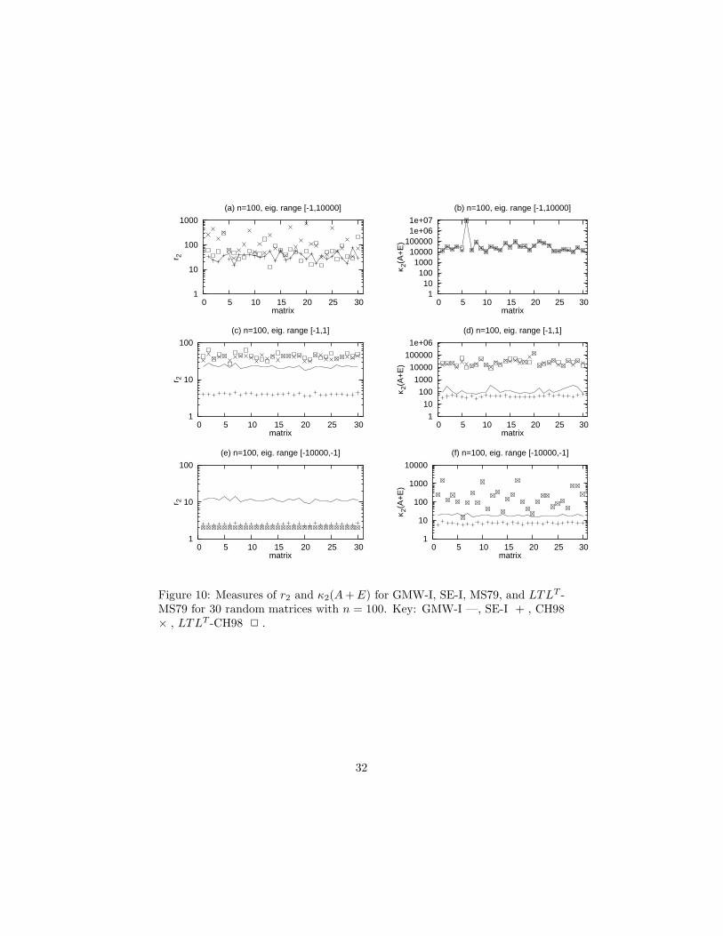
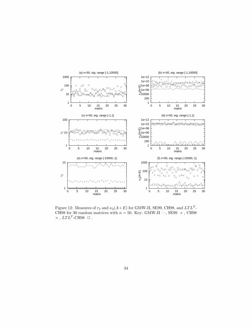
Figures 8–10 show the results of the Type-I algorithms, whereas Figures 11–
13 show results of the Type-II algorithms. We measure ‖E‖2 by r2 = ‖E‖2
|λmin(A)|as defined in (20).
Consider the Type-I algorithms. MS79 and LTLT -MS79 generally producedcomparable ‖E‖2 and condition numbers, but for matrices with eigenvalues in[−1, 10000], LTLT -MS79 achieved a smaller ‖E‖2 than MS79 in several cases.For matrices with eigenvalues in [−1, 1], SE-I outperformed the other Type-Ialgorithms by not only producing smaller ‖E‖2 but also smaller κ2(A+E). Formatrices with eigenvalues in [−10000,−1], the GMW-II produced larger ‖E‖2
than the others.Now compare the Type-II algorithms. In experiments on matrices with
eigenvalues in [−1, 10000], GMW-II and SE99 produced ‖E‖2 smaller than theothers on average. The LTLT -CH98 algorithm outperformed CH98 by usu-ally achieving a smaller ‖E‖2. For the random matrices with eigenvalues in[−1, 1], SE99 remains the best. For the random matrices with eigenvalues in[−10000,−1], CH98 and LTLT -CH98 achieved the minimal ‖E‖2.
6.2 The Benchmark Matrix
Schnabel and Eskow [15] identified a matrix that gives SE90 difficulties:
A =
1890.3 −1705.6 −315.8 3000.3−1705.6 1538.3 284.9 −2706.6−315.8 284.9 52.5 −501.23000.3 −2706.6 −501.2 4760.8
. (51)
It became one of the benchmark matrices for the modified Cholesky algorithms[5, 16]. This matrix has eigenvalues {−0.378,−0.343,−0.248, 8.24× 10³}.
29

1
10
100
1000
0 5 10 15 20 25 30
r 2
matrix
(a) n=25, eig. range [-1,10000]
1
10
100
1000
10000
100000
1e+06
0 5 10 15 20 25 30
κ 2(A
+E
)
matrix
(b) n=25, eig. range [-1,10000]
1
10
100
0 5 10 15 20 25 30
r 2
matrix
(c) n=25, eig. range [-1,1]
1
10
100
1000
10000
100000
0 5 10 15 20 25 30
κ 2(A
+E
)
matrix
(d) n=25, eig. range [-1,1]
1
10
0 5 10 15 20 25 30
r 2
matrix
(e) n=25, eig. range [-10000,-1]
1
10
100
1000
10000
0 5 10 15 20 25 30
κ 2(A
+E
)
matrix
(f) n=25, eig. range [-10000,-1]
Figure 8: Measures of r2 and κ2(A + E) for GMW-I, SE-I, MS79, and LTLT -MS79 for 30 random matrices with n = 25. Key: GMW-I —, SE-I + , CH98× , LTLT -CH98 2 .
30

1
10
100
1000
0 5 10 15 20 25 30
r 2
matrix
(a) n=50, eig. range [-1,10000]
1
10
100
1000
10000
100000
1e+06
0 5 10 15 20 25 30
κ 2(A
+E
)
matrix
(b) n=50, eig. range [-1,10000]
1
10
100
0 5 10 15 20 25 30
r 2
matrix
(c) n=50, eig. range [-1,1]
1
10
100
1000
10000
100000
0 5 10 15 20 25 30
κ 2(A
+E
)
matrix
(d) n=50, eig. range [-1,1]
1
10
0 5 10 15 20 25 30
r 2
matrix
(e) n=50, eig. range [-10000,-1]
1
10
100
1000
10000
0 5 10 15 20 25 30
κ 2(A
+E
)
matrix
(f) n=50, eig. range [-10000,-1]
Figure 9: Measures of r2 and κ2(A + E) for GMW-I, SE-I, MS79, and LTLT -MS79 for 30 random matrices with n = 50. Key: GMW-I —, SE-I + , CH98× , LTLT -CH98 2 .
31
1
10
100
1000
0 5 10 15 20 25 30
r 2
matrix
(a) n=100, eig. range [-1,10000]
1 10
100 1000
10000 100000 1e+06 1e+07
0 5 10 15 20 25 30
κ 2(A
+E
)
matrix
(b) n=100, eig. range [-1,10000]
1
10
100
0 5 10 15 20 25 30
r 2
matrix
(c) n=100, eig. range [-1,1]
1
10
100
1000
10000
100000
1e+06
0 5 10 15 20 25 30
κ 2(A
+E
)
matrix
(d) n=100, eig. range [-1,1]
1
10
100
0 5 10 15 20 25 30
r 2
matrix
(e) n=100, eig. range [-10000,-1]
1
10
100
1000
10000
0 5 10 15 20 25 30
κ 2(A
+E
)
matrix
(f) n=100, eig. range [-10000,-1]
Figure 10: Measures of r2 and κ2(A + E) for GMW-I, SE-I, MS79, and LTLT -MS79 for 30 random matrices with n = 100. Key: GMW-I —, SE-I + , CH98× , LTLT -CH98 2 .
32

1
10
100
1000
0 5 10 15 20 25 30
r 2
matrix
(a) n=25, eig. range [-1,10000]
1
100
10000
1e+06
1e+08
1e+10
1e+12
0 5 10 15 20 25 30
κ 2(A
+E
)
matrix
(b) n=25, eig. range [-1,10000]
1
10
100
0 5 10 15 20 25 30
r 2
matrix
(c) n=25, eig. range [-1,1]
1
100
10000
1e+06
1e+08
1e+10
1e+12
0 5 10 15 20 25 30
κ 2(A
+E
)
matrix
(d) n=25, eig. range [-1,1]
1
10
0 5 10 15 20 25 30
r 2
matrix
(e) n=25, eig. range [-10000,-1]
1
10
100
1000
0 5 10 15 20 25 30
κ 2(A
+E
)
matrix
(f) n=25, eig. range [-10000,-1]
Figure 11: Measures of r2 and κ2(A+E) for GMW-II, SE99, CH98, and LTLT -CH98 for 30 random matrices with n = 25. Key: GMW-II —, SE99 + , CH98× , LTLT -CH98 2 .
33
1
10
100
1000
0 5 10 15 20 25 30
r 2
matrix
(a) n=50, eig. range [-1,10000]
1
100
10000
1e+06
1e+08
1e+10
1e+12
0 5 10 15 20 25 30
κ 2(A
+E
)
matrix
(b) n=50, eig. range [-1,10000]
1
10
100
0 5 10 15 20 25 30
r 2
matrix
(c) n=50, eig. range [-1,1]
1
100
10000
1e+06
1e+08
1e+10
1e+12
0 5 10 15 20 25 30
κ 2(A
+E
)
matrix
(d) n=50, eig. range [-1,1]
1
10
0 5 10 15 20 25 30
r 2
matrix
(e) n=50, eig. range [-10000,-1]
1
10
100
1000
0 5 10 15 20 25 30
κ 2(A
+E
)
matrix
(f) n=50, eig. range [-10000,-1]
Figure 12: Measures of r2 and κ2(A+E) for GMW-II, SE99, CH98, and LTLT -CH98 for 30 random matrices with n = 50. Key: GMW-II —, SE99 + , CH98× , LTLT -CH98 2 .
34

1
10
100
1000
0 5 10 15 20 25 30
r 2
matrix
(a) n=100, eig. range [-1,10000]
1
100
10000
1e+06
1e+08
1e+10
1e+12
0 5 10 15 20 25 30
κ 2(A
+E
)
matrix
(b) n=100, eig. range [-1,10000]
1
10
100
0 5 10 15 20 25 30
r 2
matrix
(c) n=100, eig. range [-1,1]
1
100
10000
1e+06
1e+08
1e+10
1e+12
0 5 10 15 20 25 30
κ 2(A
+E
)
matrix
(d) n=100, eig. range [-1,1]
1
10
100
0 5 10 15 20 25 30
r 2
matrix
(e) n=100, eig. range [-10000,-1]
1
10
100
1000
10000
0 5 10 15 20 25 30
κ 2(A
+E
)
matrix
(f) n=100, eig. range [-10000,-1]
Figure 13: Measures of r2 and κ2(A+E) for GMW-II, SE99, CH98, and LTLT -CH98 for 30 random matrices with n = 100. Key: GMW-II —, SE99 + , CH98× , LTLT -CH98 2 .
35

Table 5: Measures of ‖E‖ and κ2(A + E) for the benchmark matrix (51).
Algorithm r2 rF κ2(A + E)
GMW81 2.733 2.674 4.50× 10⁴
GMW-I 3.014 2.739 4.51× 10⁴
GMW-II 2.564 2.489 1.64× 10⁵
SE90 2.78× 10³ 3.70× 10³ 8.858SE99 1.759 1.779 1.04× 10¹⁰
SE-I 3.346 3.289 3.61× 10⁴
MS79 3.317 2.689 3.33× 10⁴
CH98 1.659 1.345 9.88× 10⁷
LTLT -MS79 3.317 2.689 3.33× 10⁴
LTLT -CH98 1.658 1.344 6.74× 10¹⁰
LTLT -MS79, 2-phase 3.317 2.689 3.33× 10⁴
LTLT -CH98, 2-phase 1.658 1.344 8.59× 10¹⁰
LTLT -MS79, relaxed 2-phase 2.15× 10⁴ 2.03× 10⁴ 3.68× 10⁴
LTLT -CH98, relaxed 2-phase 2.15× 10⁴ 2.03× 10⁴ 7.47× 10¹⁰
The measures of ‖E‖2 and ‖E‖F in terms of r2 and rF , and the conditionnumbers κ2(A + E) are listed in Table 5 for various modified Cholesky algo-rithms, where the new methods are in boldface. This illustrates the instability ofincorporating the relaxed 2-phase strategy into LTLT -CH98 and LTLT -MS79,where the relaxation factor was µ = 0.1. In this case the instability can beresolved by dropping the relaxation factor down to µ = 10−4. However, theinstability was not extinguished for the matrices A15 1, A15 2, and A15 3 inSection 6.3, after trying several different relaxation factors.
6.3 The 33 Matrices
33 matrices, generated by Gay, Overton, and Wright from optimization problemswhere GMW81 outperformed SE90, were used by Schnabel and Eskow [16] toevaluate modified Cholesky algorithms.
Table 6 summarizes r2 = ‖E‖2
|λmin(A)| and ζ = blog10(κ2(A + E))c for the
existing algorithms in the literature, whereas Tables 7 gives the result of the newalgorithms. Matrix B13 1 is positive definite but extremely ill-conditioned, sothat we measure E by ‖E‖2 instead of r2. We see that SE90 did not perform wellon several matrices, and the r2 for CH98 is somewhat large on a few matrices(e.g., A6 7). The other methods produced a reasonable E in all cases. Forthese 33 matrices, Type-I algorithms generally resulted in better conditioningof A + E, whereas Type-II algorithms generally produced smaller ‖E‖, exceptfor SE90 and CH98.
Incorporating the special treatments from SE99 for the last 1×1 and 2×2 Schurcomplements (see (15) and (16)) into GMW-II can often produce slightly smaller
36

‖E‖2 for matrices close to positive definite. Similarly, the special treatments forSE-I in (27) and (28) can help GMW-I reduce ‖E‖2. The detailed discussion isomitted for simplicity.
7 Concluding Remarks
The modified Cholesky algorithms in this paper are categorized in Table 8,where the new methods are in boldface. Our conclusions are listed below.
1. The rationale for the algorithms in the GMW class is to bound the off-diagonal elements in L. The rationale for the algorithms in the SE classis to control the Gerschgorin circles in the Schur complements.
2. The nondecreasing strategy can be incorporated into virtually all algo-rithms which confine the modification to the diagonal. The rationale isthat it does not increase ‖E‖2 at each stage, and it may keep the subse-quent modifications smaller. It is especially favored by the Type-II algo-rithms, since it can also empirically improve the conditioning of A + E.
3. The 2-phase and relaxed 2-phase strategies are incorporated into SE90and SE99 respectively for satisfying Objective 1, whereas they are notrequired for GMW81.
4. GMW81 and its Type-II variant have ‖E‖ = O(n2). The 2-phase strategycan drop the bound to be ‖E‖ = O(n). However, it may result in excessive‖E‖2 for matrices close to being positive definite. The problem can besolved by relaxing. The situation is similar to that of SE90 and SE99. Therelaxed 2-phase strategy usually improves the modified LDLT algorithms.
5. For algorithms in the GMW class and in the SE class, the theoreticalbounds on ‖E‖2 and κ2(A + E) do not rely on pivoting. In practice,pivoting reduces ‖E‖2.
6. Our GMW-II algorithm outperforms GMW81 and GMW-I by generallykeeping ‖E‖2 smaller for the random matrices with eigenvalues in [−1, 10000],whereas GMW81 outperforms our GMW-I and GMW-II for the randommatrices with eigenvalues in [−10000,−1].
7. In our experiments, SE99 and GMW-II are the best modified LDLT al-gorithms with respect to ‖E‖ for matrices with eigenvalues in [−1, 10000],whereas SE-I generally produces ‖E‖ smaller than those for SE90 andSE99 for matrices with eigenvalues in [−10000,−1] and [−1, 1].
8. In experiments on distance matrix completion problems we noted thatincreasing the relaxation factor µ from 0.75 to 1.0 can significantly improvethe performance of GMW-II not only for random problems with 65% ormore unspecified entries but also for protein problems [7]. With thesechanges, however, Objective 2 was not satisfied as well for the 33 matricesin Section 6.3.
37

Table 6: r2 = ‖E‖2
|λmin(A)| and ζ = blog10(κ2(A + E))c of the existing methods.
Method GMW81 SE90 SE99 MS79 CH98
r2 ζ r2 ζ r2 ζ r2 ζ r2 ζ
A6 1 1.365 5 3.6e+2 1 1.079 9 2.188 5 1.094 8A6 2 4.844 3 1.175 5 1.180 7 2.304 3 1.152 7A6 3 4.847 4 1.200 5 1.208 6 2.328 3 1.164 7A6 4 2.501 5 1.275 5 1.270 8 2.541 4 1.271 8A6 5 2.347 5 6.503 3 1.448 9 4.512 5 2.257 8A6 6 1.693 8 2.947 5 1.201 10 2.757 8 1.384 8A6 7 1.953 12 4.6e+4 5 1.334 10 2.033 12 3.6e+2 8A6 8 1.953 8 6.611 5 1.138 10 2.033 8 1.030 8A6 9 1.958 8 47.221 5 1.125 10 2.031 9 1.131 8A6 10 5.887 8 5.4e+6 0 1.076 11 6.636 8 3.675 8A6 11 2.334 8 7.3e+6 0 1.648 7 6.049 8 3.570 8A6 12 4.847 4 1.200 5 1.208 6 2.328 3 1.164 7A6 13 2.180 2 1.322 5 1.322 6 3.115 2 1.558 8A6 14 4.847 4 1.200 5 1.208 6 2.328 3 1.164 7A6 15 5.188 1 1.090 5 1.090 5 2.146 1 1.073 7A6 16 2.180 2 1.322 5 1.322 6 3.115 2 1.558 8A6 17 1.527 2 1.246 5 1.246 6 2.752 2 1.376 8A13 1 2.253 10 8.9e+3 5 1.183 10 3.847 9 57.944 8A13 2 2.599 8 1.5e+4 5 1.317 10 2.805 8 4.716 8A15 1 2.421 9 2.5e+7 5 1.895 11 4.165 10 5.954 8A15 2 2.375 9 3.9e+5 3 1.449 10 2.834 10 9.948 8A15 3 1.957 6 2.183 5 1.503 10 3.991 7 2.021 8B6 1 4.901 3 52.418 0 1.773 8 3.024 2 1.512 8B6 2 4.495 2 45.866 0 2.315 7 4.200 3 2.100 8B7 1 1.666 2 3.450 2 1.067 2 2.263 2 1.131 8B7 2 1.932 2 11.005 0 1.309 7 3.320 2 1.660 7B7 3 1.967 2 6.998 0 1.227 6 2.669 2 1.334 7B7 4 1.929 2 5.325 1 1.189 6 2.619 2 1.310 7B8 1 4.164 12 8.7e+2 5 1.279 10 4.164 12 9.705 8
B13 1 (abs.) 0 9 27.15 5 0 9 0 9 0.215 7B13 2 1.762 7 7.846 5 1.291 10 3.887 7 1.949 8B26 1 9.833 1 2.234 3 2.364 7 28.293 2 14.146 8B55 1 3.504 1 1.714 5 1.714 6 95.603 3 47.802 9
38

Table 7: r2 = ‖E‖2
|λmin(A)| and ζ = blog10(κ2(A + E))c of the new methods.
Method GMW-I GMW-II SE-I LTLT−MS79 LTL
T−CH98
r2 ζ r2 ζ r2 ζ r2 ζ r2 ζ
A6 1 1.989 4 2.111 5 2.181 4 2.153 5 1.077 11A6 2 4.265 3 3.881 2 2.360 3 2.306 3 1.153 10A6 3 5.160 2 2.528 11 2.416 2 2.323 3 1.162 10A6 4 2.574 3 1.290 10 2.541 3 2.756 4 1.378 10A6 5 3.120 4 1.647 10 2.895 4 3.111 4 1.556 10A6 6 2.363 7 1.418 5 2.403 6 2.754 8 1.377 10A6 7 2.189 11 1.331 10 2.109 10 2.032 11 1.352 10A6 8 2.189 7 1.051 10 2.277 7 2.032 8 1.016 10A6 9 2.179 8 1.064 10 2.249 8 2.031 9 1.016 10A6 10 4.883 7 4.399 6 2.031 7 2.438 8 1.219 11A6 11 2.550 7 2.311 7 1.737 7 3.604 8 1.802 11A6 12 5.160 2 2.528 11 2.416 2 2.323 3 1.162 10A6 13 3.289 1 2.971 1 2.643 1 2.911 2 1.455 11A6 14 5.160 2 2.528 11 2.416 2 2.323 3 1.162 10A6 15 5.338 1 2.666 11 2.181 1 3.195 1 1.597 10A6 16 3.289 1 2.971 1 2.643 1 2.911 2 1.455 11A6 17 2.713 1 2.461 1 2.492 1 2.519 2 1.259 11A13 1 2.288 10 1.198 10 2.257 9 2.258 9 1.184 10A13 2 2.767 8 1.406 10 2.627 8 2.642 8 1.324 10A15 1 5.718 9 5.372 8 3.815 8 4.886 10 2.444 11A15 2 2.925 8 2.728 8 2.887 8 2.834 10 1.432 10A15 3 3.953 6 3.789 6 3.006 6 2.689 7 1.344 11B6 1 2.817 2 2.512 2 3.545 2 2.224 2 1.112 11B6 2 3.367 2 3.061 2 4.630 2 2.398 2 1.199 11B7 1 2.062 2 1.663 2 2.005 2 2.019 2 1.010 11B7 2 2.721 2 1.449 11 2.618 1 7.217 2 3.609 11B7 3 2.610 2 1.377 11 2.453 1 6.795 2 3.397 11B7 4 2.538 2 1.337 11 2.378 1 2.683 2 1.342 10B8 1 4.164 12 2.087 11 2.548 10 4.022 12 2.017 11B13 1 0 9 0 9 0 9 0 9 0 9B13 2 5.273 7 4.859 5 2.581 6 2.405 7 1.203 10B26 1 6.639 1 3.721 2 5.827 1 17.386 2 8.693 11B55 1 3.504 1 1.752 10 3.428 1 11.289 1 5.645 10
39

Table 8: Categories of various modified Cholesky algorithms.
Category Type I Type II
LDLT GMW81, GMW-I, SE-I GMW-II, SE90, SE99LBLT MS79 CH98LTLT LTLT -MS79 LTLT -CH98
For the modified LBLT factorizations and our new approach via the LTLT
factorization, the concluding remarks are as follows.
1. In worst cases, MS79 and CH98 take Θ(n3) time more than the standardCholesky factorization and therefore do not satisfy Objective 4, whereasour LTLT -MS79 and LTLT -CH98 algorithms guarantee O(n2) modifica-tion expense.
2. In experiments on random matrices with eigenvalues [−1, 10000], LTLT -MS79 and LTLT -CH98 usually produce an ‖E‖2 smaller than MS79 andCH98, respectively. Our new approach outperforms the modified LBLT
algorithms in the literature, not only by guaranteeing the O(n2) modifica-tion cost, but also by usually producing a smaller ‖E‖2 for matrices closeto being positive definite.
3. It is possible to incorporate the 2-phase strategy or the relaxed 2-phasestrategy into LTLT -MS79 and LTLT -CH98, but the resulting algorithmsmay produce unreasonably large ‖E‖, as shown in Figure 7 and discussedin Section 6.2, respectively.
4. The modification arguments δ listed in Table 1 aimed at the satisfactionthe four objectives. In practice, especially for Type-II algorithms, theycould be too small and affect the conditioning, from which difficulty mayarise. In our experiments on random distance matrix completion problems[7], difficulty was apparent for CH98 and LTLT -CH98. To amend theproblem, we increased the modification tolerance parameter δ to τη (usedby SE90) for both CH98 and LTLT -CH98.
The best algorithm, modification tolerance δ, and relaxation factor µ forthe relaxed 2-phase strategy depend on the optimization problem. Experimentsmay be required to tune δ and µ for each application.
Acknowledgement
The authors thank Betty Eskow for very helpful discussions and for making hercode from [16] available to us.
40

References
[1] J. O. Aasen. On the reduction of a symmetric matrix to tridiagonal form.BIT, 11(3):233–242, 1971.
[2] C. Ashcraft, R. G. Grimes, and J. G. Lewis. Accurate symmetric indefinitelinear equation solvers. SIAM J. Matrix Anal. Appl., 20(2):513–561, 1998.
[3] J. R. Bunch and L. Kaufman. Some stable methods for calculating inertiaand solving symmetric linear systems. Math. Comp., 31:163–179, 1977.
[4] J. R. Bunch and B. N. Parlett. Direct methods for solving symmetricindefinite systems of linear equations. SIAM J. Numer. Anal., 8(4):639–655, 1971.
[5] S. H. Cheng and N. J. Higham. A modified Cholesky algorithm basedon a symmetric indefinite factorization. SIAM J. Matrix Anal. Appl.,19(4):1097–1110, 1998.
[6] H.-r. Fang and D. P. O’Leary. Stable factorizations of symmetric tridiagonaland triadic matrices. SIAM J. Matrix Anal. Appl., to Appear, 2006.
[7] H.-r. Fang and D. P. O’Leary. Dimensional relaxation for distance matrixcompletion problems. Technical report, Computer Science Department,Univ. of Maryland, College Park, MD, in preparation.
[8] A. Forsgren, P. E. Gill, and W. Murray. Computing modified Newtondirections using a partial Cholesky factorization. SIAM J. Sci. Comput.,16(1):139–150, 1995.
[9] P. E. Gill and W. Murray. Newton-type methods for unconstrained andlinearly constrained optimization. Math. Programming, 28:311–350, 1974.
[10] P. E. Gill, W. Murray, and M. H. Wright. Practical Optimization. AcademicPress, 1981.
[11] N. J. Higham. Stability of the diagonal pivoting method with partial piv-oting. SIAM J. Matrix Anal. Appl., 18(1):52–65, 1997.
[12] R. A. Horn and C. R. Johnson. Matrix Analysis. Cambridge UniversityPress, 1985.
[13] J. J. More and D. C. Sorensen. On the use of directions of negative curva-ture in a modified Newton method. Math. Programming, 16:1–20, 1979.
[14] B. N. Parlett and J. K. Reid. On the solution of a system of linear equationswhose matrix is symmetric but not definite. BIT, 10(3):386–397, 1970.
[15] R. B. Schnabel and E. Eskow. A new modified Cholesky factorization.SIAM J. Sci. Stat. Comput., 11:1136–1158, 1990.
41

[16] R. B. Schnabel and E. Eskow. A revised modified Cholesky factorizationalgorithm. SIAM J. Optim., 9(4):1135–1148, 1999.
[17] G. W. Stewart. The efficient generation of random orthogonal matrices withan application to condition estimation. SIAM J. Numer. Anal., 17:403–409,1980.
42