MODELLING SMALLER UK CORPORATIONS: A PORTFOLIO ANALYSIS

OXFORD BULLETIN OF ECONOMICS AND STATISTICS, 53,4(1991)0305-9049 S3.00

MODELLING SMALLER UK CORPORATIONS:A PORTFOLIO ANALYSIS

Donald A. Hay and Helen Louri*

I. INTRODUCTION

The research reported in this paper has attempted to model the balance sheetbehaviour of smaller UK corporations. A mean-variance model was used afterextensive experimentation with other portfolio models and different samples.In a previous paper, Hay and Louri (1989), we applied the mean-varianceframework to balance sheet items of a sample of unquoted UK firms. Therewas clear evidence of interdependence between balance sheet items. Thesuccess of this application encouraged us to try a similar framework forquoted corporations, taking into account the differences between the twotypes of firm, particularly the ability of quoted corporations to issue newequity, and the separation of ownership and control.

Following the seminal contribution of Brainard and Tobin (1968), aconsiderable literature has developed on the application of portfolio theoryto the balance sheets of financial institutions. Examples of this literature areParkin et aL (1970), Parkin (1970), Sharpe (1973), Courakis (1974, 1975 and1980). Much of the earlier literature is critically surveyed by Courakis (1988).The message of these studies is that, according to portfolio theory, assets andliabilities are simultaneously determined in the balance sheets of financialinstitutions, and that this simultaneity should be explicitly addressed ineconometric analyses. The three key assumptions of the theory are: thedecision taker seeks to maximize the expected utility of wealth at some termi-nal date, the choice between alternative portfolios is determined solely byexpected return and risk (proxied by the mean and variance of returns), andthe decision takers are quantity setters taking as parametric the vector of sto-chastic yields (costs) on different assets (liabilities).

Given the success of portfolio models of financial institutions, it is surpris-ing that a similar approach has not generally been taken to the determinants

*We are grateful to Paul Horsnell for programming assistance, to A. Banerjee for econo-metric advice, to A. Courakis for discussions, to anonymous referees for criticism and sugges-tions on how to improve the paper, and to the Institute of Economics and Statistics, Oxford, forresearch facilities. Helpful comments and suggestions were received from seminar audiences atEUT, Florence and at Oxford. The research is supported by the SPES programme of theEuropean Community, Contract Number ERB SPES CT9 15000.

425

426 BULLETIN

of the balance sheets of firms. Exception are the papers by Dhrymes andKurz (1967), Hay and Morris (1984), and Mueller (1967), Grabowski andMueller (1972), which, however, use no formal portfolio model analysis.Other studies (Bosworth, 1971; Taggart, 1977; Friedman, 1979; Chowdhury,Green and Miles, 1986; Croasdale, 1988) have restricted their attention tothe financial variables (loans, trade debt and credit, working capital, newequity issues) in firms balance sheets, presumably on the basis that decisionsabout real variables (fixed capital, stocks and work in progress), are prior.The firm decides on its investment and production plan first, and then seeksan optimal financing package to enable it to put that plan into effect. With theexceptions of Taggart and Chowdhury et al. these studies utilize aggregatedata for the whole corporate sector. Once again, there is no analysis of aformal portfolio model.

The reluctance to pursue a full portfolio model of the balance sheets offirms can be justified in two ways. Friedman (1979, p. 135) gives his judge-ment that 'as yet there exists no satisfactory comprehensive theory of how thefirm jointly determines' all the different items in the balance sheet. It isevident that he regards existing portfolio theory as being inadequate to thetask.

Alternative justifications rely on the difficulty of matching the assumptionsof the theory to the reality of firms' experience. First, it is hard to justify theuse of period analysis in a situation where a firm may alter its holdings ofassets and liabilities continuously. One can appeal to the idea of a planningperiod, and to the existence of adjustment costs preventing instantaneousadjustment. But there is no reason to believe that either planning periods oradjustment costs are the same across all balance sheet items. (Nor that theplanning period is one year, and that the terminal date coincides with theannual balance sheet drawn up for accounting purposes: but we have to useannual balance sheets in our empirical work.)

Secondly, the analysis is open to theoretical objection. The analysis arises,in the case of the portfolio model we are considering, from the assumptionthat the agents are risk averse, with preferences described by a negativeexponential utility function in wealth or profits. But the shareholders in aquoted firm are likely to hold equity as part of a diversified portfolio ofwealth. They will be interested in the covariance risk of their holding, andquite unconcerned about the variance risks implied in the balance sheet of thefirm. But for the managers of the firm, the variance risks may be very sig-nificant. They are likely to have substantial human capital sunk in the firm,and may have equity holdings or equity linked incentives which constitute asignificant part of their private wealth. In particular, where managerial effortis not observable, a poor financial performance may be taken by the share-holders as a signal of slack, even where it arises from shocks outside thecontrol of the managers. The danger for the managers is that shareholderswill be responsive to takeover bids, leading to their dismissal, with con-sequent loss of their human capital in the firm. Managers are therefore likely

MODELLING SMALLER UK CORPORATIONS 427

to be motivated by their own risk aversion in structuring the balance sheet.They will also wish to maximize expected profit in order to enhance the valueof their human capital, and to maximize returns on their own equity or equitylinked incentives.

A third assumption of the theory is that of price-taking, quantity-settingbehaviour applied to all items in the balance sheet. In fact, the firm will haveconsiderable discretion over the returns to be earned on its physical invest-ment; pricing and marketing decisions can affect returns in the short run, andR & D in the long run. We have to imagine that the firm operates in a numberof broadly defined markets which give rise to a large number of investmentopportunities, all of which yield an expected risk-adjusted rate of return,given appropriate expenditures on marketing and product development. Thefirm picks a few projects to coincide with its existing expertise. The analysisof this paper presumes that this description of firms' investment behaviour isbroadly correct.

The empirical focus of this paper is on smaller UK quoted companies.Econometric experiments with a sample of firms drawn randomly from thequoted sector were unsatisfactory: conventional measures of goodness of fitsuggested that little of the variance in the data was being explained by themodel. One possibility is that the larger quoted companies are managerial,motivated as much by growth of the firm as by the level of profit. Ourtentative conclusion is that it is a mistake to expect a single model to beappropriate for all quoted firms.' Given our previous success in applying themodel to unquoted finns, we restricted our sample selection, for this paper, tofirms of similar size. We also note that while in principle the firms are able tomake new equity issues, in practice few do so, due to the high transactionscosts. They are, therefore, similar to unquoted firms in this respect.

The plan of the paper is conventional. In Section II we briefly review thetheory; in Section III we deal with specification and data definitions; inSection IV we examine the results. A final section summarizes our con-clusions.

II. PORTFOLIO MODELS

The portfolio model used in this paper has been described fully by Courakis(1974, 1980), so the exposition here will be brief. The fundamental assump-tion is that the preferences of agents can be described by a negativeexponential utility function in profits (ir):

U( .r) = a - c exp( - b r) with a, b, e> O

The proposition that the objectives of firms may vary according to characteristics such assize, organizational structure and pattern of ownership is well established in the literature. For acritical review see Hay and Morris (1991), Chapter 9.

428 BULLETIN

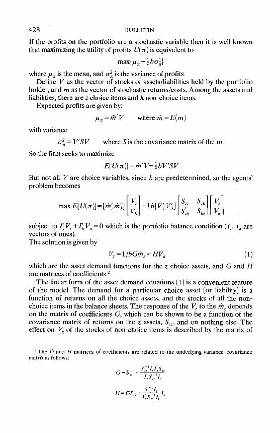
lithe profits on the portfolio are a stochastic variable then it is well knownthat maximizing the utility of profits U( 2r) is equivalent to

max{u - ba,}where 1u is the mean, and u is the variance of profits.

Define V as the vector of stocks of assets/liabilities held by the portfolioholder, and m as the vector of stochastic returns/costs. Among the assets andliabilities, there are z choice items and k non-choice items.

Expected profits are given by:

p=th'V whereth=E(m)

with variance

Ur= V'SV where S is the covariance matrix of the m.

So the firm seeks to maximize

E[U(2r)1= th'VbV'SVBut not all V are choice variables, since k are predetermined, so the agents'problem becomes

Szk11l[Vkj LSZk SkkjLVkj

subject to I' V + "k Vk = O which is the portfolio balance condition ('r. 'k arevectors of ones).The solution is given by

V=1/bGthHV,, (1)

which are the asset demand functions for the z choice assets, and G and Hare matrices of coefficients.2

The linear form of the asset demand equations (1) is a convenient featureof the model. The demand for a particular choice asset (or liability) is afunction of returns on all the choice assets, and the stocks of all the non-choice items in the balance sheets. The response of the V to the th dependson the matrix of coefficients G, which can be shown to be a function of thecovariance matrix of returns on the z assets, and on nothing else. Theeffect on J" of the stocks of non-choice items is described by the matrix of

2 G and H matrices of coefficients are related to the underlying variance-covariancematrix as follows:

G=ST)z

H = GSZk+ 'k


coefficients, H, which is a function of the covariance matrix of returns onchoice and non-choice items, SZk, as well as S. Note however that the level ofreturns on the non-choice assets does not feature: it is the composition of thenon-choice items, and their contribution to the riskiness of the portfoliowhich matters.

The mathematical properties of the G and H coefficient matrices areimportant for empirical applications of the model:

(i) symmetry: G is symmetric(il) homogeneity: an equal change in the ratios of returns on all choice

assets leaves the relative demands for these assets unchangedCournot aggregation: all asset adjustments following a change inreturns must be consistent with keeping the balance sheet in balancenon-negative own rate coefficients: an increase in expected yield on anasset, ceteris paribus, will never lead to a decrease in the stock of thatasset held

(y) Engle aggregation: a consequence of the balance sheet constraint. Achange in the stock of a non-choice asset brings about changes indemand for the different choice set assets which add up to the initialchange.

These restrictions may be tested as part of the empirical evaluation of themodel. Properties (iii) and (y) are automatically satisfied by the balancesheets. Homogeneity and symmetry can be tested by comparing restrictedand unrestricted versions of the model.

Finally, we note that this portfolio model, with its linear asset demandfunctions, is an outcome of the particular assumptions made. Courakis(1989) has shown that other specific utility functions, with similar generalproperties, do not give such convenient asset demand functions. We thereforeneed to be particularly cautious about interpreting our empirical results inSection IV.

III. SPECIFICATION AND DATA

Published balance sheets of quoted companies contain a great deal of detailabout the firm's assets and liabilities. Much of the detail is due to accountingconventions which possibly have little significance for firm behaviour. Foranalysis we consolidated items to arrive at the following simplified balancesheet for each enterprise:

Assets Liabilities

Net physical capital (KL+ NI) Shareholders' funds (SH)Stocks and w.i.p. (SL+ DST) Revaluation reserve (RR)Trade debt (TD) Loans (LA)Working capital (WK) Trade credit (TC)

Total assets are, of course, equal to total liabilities.

430 BULLETIN

We note the following features of this simplified balance sheet:

Net physical capital is divided into two items: KL is the net physicalassets inherited from the previous period: NI is net investment in thecurrent period.Stocks and work-in-progress are similarly divided into stocks carriedforward from the previous period, SL, and net additions to stocks inthe current period, DST.Working capital (WK) is a netting out of a miscellaneous collection ofshort-term assets and liabilities, such as short-term deposits at thebank and cash, dividends declared but not paid, unpaid tax liabilities.The rationale for netting out these items is that the level of any one isprobably an accident of the day on which the firm's books were closedfor the year. But the net value of working capital is certainly a numberwhich will concern the managers and the short-term creditors of thefirm as an indicator of its ability to meet immediate obligations and tocontinue operations. It is therefore likely to represent a consciouspolicy decision by the firm.Revaluation reserve (RR). As explained below, the accounts wereadjusted for inflation. Different adjustments to the two sides of thebalance sheet had the effect of unbalancing the account. This wasrectified by adding a revaluation reserve, as a liability, to restore thebalance. The inflation adjusted value of the assets net of loans andtrade credit usually exceeded the inflation adjusted value of share-holders funds (both equity capital and accumulated reserves fromretentions). The revaluation reserve therefore represents a capital gainto the shareholders, which is entered as a liability in the balance sheet.(Note that this value for the shareholders interest (SH plus RR) differsfrom the stock market value of the shareholder's equity: assets havebeen revalued solely on the basis of inflation of prices of capitalgoods, and not at all on the basis of the rents those assets can earn forthe enterprise.)

The data consist of profit and loss accounts, and balance sheets, for 39 UKquoted companies in 13 two-digit SIC sectors over the period 1960-85.Data were not always available over the entire period: on average there were17 annual observations for each firm. All the accounts were adjusted to 1980prices.4

source of the data is the Cambridge DTI Databank of Company Accounts, which givesstandardized (and detailed) accounting data for the great majority of companies quoted on theUK stock market since the 1950's. The data is fully described in Goudie et al. (1985). A dataappendix with details of the 39 firm sample and the procedures adopted for adjusting the datafor inflation is available from the authors on request.

Inflation adjusted capital stock was derived by calculating gross investment in each year atconstant prices, and by assuming that the true rate of depreciation in each year is given by theratio of depreciation to book value of assets in that year. With the further assumption that thebook value of assets shown in the first set of accounts for each firm (usually 1960) was anaccurate base value, the rest of the series was built up by deducting depreciation and addinggross investment in each year (both at constant prices).


Application of the model of portfolio choice in Section II requires identifi-cation of the pre-determined variables in the balance sheet, KL, SL, SH andRR are so identified. KL is the net physical capital inherited from theprevious period: it is assumed pre-determined on the grounds that muchrepresents assets that are specific to the firm (sunk'), and that the imperfec-tion of markets for second hand capital assets does not make disposal a viableoption. (Only trade investments in other firms are likely to be realizable: thesehave been netted out of both KL and SH). The inclusion of SL (stocks andw.i.p. inherited from the previous period) in the list of predetermined var-iables is more debatable. It seems likely that the level of stocks is in principlea decision variable of the firm, and that the adjustment period is less than oneyear in the typical case. However including SL as a predetermined variableenables us to test the hypothesis of adjustment within a year. Shareholdersfunds (SH) and the revaluation reserve (RR) are combined to give a singlevariable (SR) representing shareholders interests in the enterprise. In princi-ple, given that the firms in the sample are quoted, SH might be modelled as achoice variable. However, in practice, small quoted firms seldom raise newequity capital, relying on retentions. Furthermore, given the dividend smooth-ing behaviour of quoted firms, retentions are a residual after other claims onprofits, rather than a choice variable, at least in the short run. We have, there-fore, assumed that SR is predetermined. In any case, Valentine (1973) hasshown that no bias in estimation should arise from assuming that an endo-geous item in the balance sheet is predetermined. Information about returnson an item is implicit in its level, and the covariances between returns on theitem and returns on choice assets/liabilities are implicit in the coefficients H(see footnote 1 for the definition of H).

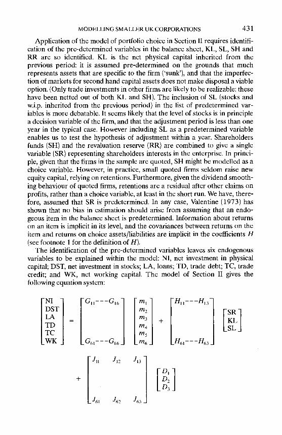
The identification of the pre-determined variables leaves six endogenousvariables to be explained within the model: NI, net investment in physicalcapital; DST, net investment in stocks; LA, loans; TD, trade debt; TC, tradecredit; and WK, net working capital. The model of Section II gives thefollowing equation system:

N1 G11---G16 - m1

DST m2 [SRLA m3 + IKLTD m4 [SLTC 1-fl5

WK G(J---G66_ - _H61---H63

+

-J11 "12

._J61 J62

l3 -

J63

[D1ID[D3

432 BULLETIN

Note that the G matrix coefficients are those of equation (1) in Section IIscaled by the factor 1/b, and that D1 is a constant, and D2 and D3 are dummyvariables for firm specific fixed effects, given that our sample includes threefirms in each sector. Balance sheet items are entered with the appropriatesign: positive for an asset, negative for a liability.

The identification of the rates of return/costs of borrowing (m1 ... m6) foreach of the assets/liabilities poses considerable difficulties. The followingrepresent a very considerable concession to data availability:

return on investment: ratio of the average increase in post-tax profitsover two subsequent years, to investment in the current year (all appropri-ately deflated). The problems of the use of accounting profit ratios tomeasure economic returns are well-documented (Edwards, Kay and Mayer,1986). We have attempted to minimize the difficulties by modelling netinvestment, so that m is defined as the incremental profit rate. It is by nomeans a perfect proxy for economic rates of return.5

returns to investment in stocks and work-in-progress: the inflation rateof producer prices in the respective sector' less the general inflation rate, onthe basis that a return to keeping stocks is the expected relative rate of pricesincrease.7 In a review of inventory analysis, Blinder and Maccini (1991)identify alternative models of inventory behaviour. The first is a productionsmoothing or buffer stock model, in which inventory investment reflectspartial adjustment to desired inventory plus partial correction of un-anticipated movements in stocks arising from sales shocks. They note thatempirically this model does not perform too well. The alternative is the (S, s)model, where the firm has an upper (S) and lower bound (s) on the quantityof stocks that it holds. When stocks fall to the lower bound an order is placedwhich will take the firm back up to the upper bound level. Inventories held ata particular time will be determined by the point reached by the firm in thiscycle of running down inventories and then restocking. The expected level ofstock will be given by the average of the two bounds. The upper bound willbe determined by inventory theoretic models which trade off carrying costsagainst the increased fixed costs of more frequent replenishments of stocks.The buffer stock model applies most obviously to inventories of finishedproducts. The (S, s) model is more appropriate for inventories of raw

We experimented with other measures, such as the current profit rate on capital, as a signalof returns to the firm, but without improving the econometric results.

data appendix referred to in footnote 3 also gives the data sources for inflation ratesused in defining the returns (costs) to assets (liabilities). Here we note the main sources as theofficial publications: Monthly Digest of Statistics, Economic Trends, Bank of England QuarterlyBulletin.

tax treatment of holdings gains on stocks is complex (Kay and King, 1986, pp. 200-1).Until 1973, stock appreciation was taken into accounting profits and taxed accordingly. In theearly 1970's high inflation rates gave rise to high accounting profits based on stock apprecia-tion: but firms lacked the financial resources to pay the tax on these paper profits. In 1974 (andmade retrospective to include 1973), stock relief was introduced. Under this scheme taxablestock appreciation was limited to 10 percent of gross trading profits. Stock relief was abolishedin 1984.


materials and other inputs. Work-in-progress is determined, in part at least,by the nature of the production process. It is evident that the holding gainsand losses can only capture one element in the determination of the level ofinvestment in inventories and work in progress. But other elements arecaptured elsewhere in the equation. The buffer stock model is picked up inthe lagged stock variable (SL). Work in progress is determined by the level ofactivity in the firm which is proxied by lagged capital (KL), and lagged stocks(SL). The carrying cost of inventories is picked up by m3, the cost of borrow-ing, which is described below. Finally, omitted variables are allowed for, inthis equation and in all the other equations of the system, by the addition of aconstant term.

costs of loans: minimum lending rate (or other base rate) net ofcorporation-tax relief, less the rate of inflation. There is no means of makingan appropriate adjustment for the premium over base rate that firms willnormally have to pay on their borrowing.8

return on trade debt: atmualized 3-month certificate of deposit (CD)rate less the inflation rate. A direct measure of the return on trade debt is notavailable. In extending credit to a customer, the firm is deferring receipt of thepayment: it will therefore seek to add to the price the full opportunity cost ofdeferred receipts. The CD rate is an opportunity cost rate, i.e. the return on ashort-term money market investment.

cost of trade credit: buying rate for trade bills averaged over the yearless inflation. The logic follows that for trade debt: if the firm issues a tradebill (i.e. a promise to pay at a specified future date), then the suppliers candiscount the bill to obtain cash immediately. Knowing the discount rate, thesupplier will adjust the price accordingly. So the implicit cost to the firm ofborrowing in this way is the discount rate. We do not expect m4 and m5 topick up all the determinants of the level of trade debt and trade credit. Butonce again, the general scale of the firms operations is captured by KL andSL, and other omitted variables by the inclusion of a constant in theequations.

return on net working capital: the return on cash assets is the negativeof the inflation rate.

To estimate the equation system we used the multivariate seeminglyunrelated regression technique. This technique minimizes the negative of thelog likelihood function to give maximum likelihood estimates. In multivariateregression the log-likelihood function includes the log of the determinant ofthe covariance matrix of the disturbances. Since disturbances are expected tobe correlated across the equation system, then the technique gives moreefficient estimates than single equation techniques.

The theory imposes restrictions on the matrices of G, H and J coefficientsin the equation system, which were incorporated as follows:

8We assume that the firms in the sample expected to earn sufficient profits to be able tobenefit from the tax relief on interest payments. It was not possible to ascertain whether any ofthe firms was in fact tax exhausted' for any part of the period of analysis.

434 BULLETIN

Cournot aggregation and (y) Engel aggregation. Balance sheetconstraints imply that the six equation are not independent. So the WKequation is omitted and its coefficients calculated from the coefficients of thefirst five: for examples, G61 = - G11 - G21 - G31 - G41 - G51, H62 =-1 -H12 -H22 -H32 ''42 -H52, J51 = -J11 -J21 -J31 -J41 -J51.

(i) symmetry and (ii) homogeneity require G = G11, andG.6 = -[G11 + G.2 + G13 + G14 + G15] for each row j in the G matrix. Theserestrictions, which are crucial to the performance of the portfolio model as awhole, are tested by comparing restricted and unrestricted versions. If therestricted version has N fewer coefficients than the unrestricted, theappropriate test is to compare the log-likelihood ratio (computed as twice thedifference in the sample log likelihood) with the Chi-square critical values forN degrees of freedom.

The requirement that the own-rate coefficients should be non-negative (G11 0) is not imposed: we regard the performance of the model inthis respect as an indicator of its applicability.

IV. SAMPLE SELECTION AND RESULTS

As noted in Section I, the sample consists mainly of smaller UK companies.Selection was determined by a number of criteria.9 We selected firms whose'history', in terms of movement in total assets and liabilities, appearedrelatively stable, excluding firms which exhibited rapid growth or decline, orwhose fortunes fluctuated markedly. Rapid growth is often a sign of a merger-intensive firm, and the conventions on accounting for acquisitions can giverise to distortion in the balance sheets of the acquiring firm. Sharp declines infortune may change the underlying behaviour of managers. In particular, ifthe firm is close to bankruptcy, managers may be prepared to take con-siderable risks, and the risk averse utility function may no longer beappropriate. The second criterion was that the firms within a sector shouldnot be too different in size. The concern was to avoid problems of hetero-scedasticity in the system of equations which might prove difficult to correctfor. The third criterion is that the firm should have as many years as possible,and at least ten years, of continuous data in the period 1960-85 without achange in accounting practice (e.g. revaluations). These criteria left us withlittle choice of firms to include in most sectors: so the question of randomsampling did not arise. Our sample was 39 firms, three in each of 13 sectors.

initial sample made no attempt to select firms on any other basis than the availability ofdata. The full six equation model described in Section III was then applied. The results werevery unsatisfactory: few of the G matrix coefficients were significant, and conventionalmeasures of goodness-of-fit suggested that little of the variance was being explained by themodel. It was these poor results that led us to be more selective in the choice of firms, asexplained in the text.


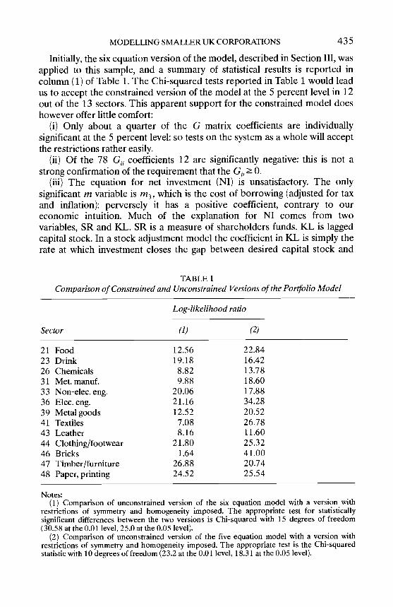
Initially, the six equation version of the model, described in Section III, wasapplied to this sample, and a summary of statistical results is reported incolumn (1) of Table 1. The Chi-squared tests reported in Table 1 would leadus to accept the constrained version of the model at the 5 percent level in 12out of the 13 sectors. This apparent support for the constrained model doeshowever offer little comfort:

(j) Only about a quarter of the G matrix coefficients are individuallysignificant at the 5 percent level: so tests on the system as a whole will acceptthe restrictions rather easily.

Of the 78 G. coefficients 12 are significantly negative: this is not astrong confirmation of the requirement that the G, 0.

The equation for net investment (NI) is unsatisfactory. The onlysignificant m variable is m3, which is the cost of borrowing (adjusted for taxand inflation): perversely it has a positive coefficient, contrary to oureconomic intuition. Much of the explanation for NI comes from twovariables, SR and KL. SR is a measure of shareholders funds. KL is laggedcapital stock. In a stock adjustment model the coefficient in KL is simply therate at which investment closes the gap between desired capital stock and

TABLE 1Comparison of Constrained and Unconstrained Versions of the Portfolio Model

Notes:Comparison of unconstrained version of the six equation model with a version with

restrictions of symmetry and homogeneity imposed. The appropriate test for statisticallysignificant differences between the two versions is Chi-squared with 15 degrees of freedom(30.58 at the 0.01 level, 25.0 at the 0.05 level).

Comparison of unconstrained version of the five equation model with a version withrestrictions of symmetry and homogeneity imposed. The appropriate test is the Chi-squaredstatistic with 10 degrees of freedom (23.2 at the 0.01 level, 18.31 at the 0.05 level).

Sector

Log-likelihood ratio

(1) (2)

21 Food 12.56 22.8423 Drink 19.18 16.4226 Chemicals 8.82 13.7831 Met. manuf. 9.88 18.6033 Non-elec. eng. 20.06 17.8836 Elec.eng. 21.16 34.2839 Metal goods 12.52 20.5241 Textiles 7.08 26.7843 Leather 8.16 11.6044 Clothing/footwear 21.80 25.3246 Bricks 1.64 41.0047 Timber/furniture 26.88 20.7448 Paper, printing 24.52 25.54

436 BULLETIN

capital stock inherited from the previous period. To sum up, the model onlycaptures the adjustment lag, it cannot tell us about the determinants ofdesired capital stock.

(iv) If ¡V can be used as a rough indicator of the goodness of fit, then it isevident that the equations for LA, TD and TC on average perform muchbetter than those for NI or DST.

(y) The six-equation version was also run using all the firms, but includingsectoral dummies. Virtually none of the G matrix coefficients weresignificant.

These less than satisfactory results led us to experiment with a fiveequation version of the model with the net investment equation deleted.There are a number of reasons why net investment might not enter the samedecision set as the other elements in the balance sheet which are underconsideration. One is that the decision and implementation lag for investmentis likely to be longer than for investment in inventories, borrowing, tradecredit and trade debt. Within a particular year the firm may be committed toan investment plan, which is therefore regarded as predetermined when itcomes to short-term decisions. This hypothesis can also be interpreted asreflecting managerial objectives of growth. The firm is committed to a long-run growth path involving an investment plan, and then adjusts other var-iables accordingly. This is not to suggest that the firm does not take the costof capital into account in deciding its growth path. Indeed net investmentequations run on their own had the appropriate signs on the cost of loans, andon profits (interpreted as a source of internal finance).

The results for the five equation model are given in Tables 2 and 3. Table 2reports an experiment with data pooled from all the sectors and with sectoraldummies included:

Six out of the 15 G matrix coefficients are significant, and the restric-tions of homogeneity and symmetry are accepted at the 1 percent level (Chi-squared 22.4, critical value 23.1). Of the 5 G.1 coefficients, two are positiveand significant (investment in stocks and trade debt equations): the otherthree are negative, but not significant.

The equation for investment in stocks (DST) is less well determinedthan the other equations. This may reflect the effect of sales shocks or may bedue to omitted determinants not captured by rates of return or the predeter-mined variables. It is however possible to interpret the equation coefficientsplausibly. The level of inventories is adjusted upwards when the relative priceof the output is expected to rise, and when returns to trade debt increase (ifthe firm is extending more credit, its activity level rises, and therefore it willcarry more stocks). An increase in the inflation rate will lead to an increase ininventories, presumably reflecting a shift out of money assets into real short-term assets. The signs of the coefficients on the predetermined variables areas expected, with an increase in shareholders funds enabling the firm to holdmore stocks, and an increase in net investment (signalling an increase inactivity) being complementary with an increase in investment in stocks. The

TA

BL

E 2

Five

Equ

atio

n V

ersi

on o

f th

e M

odel

: All

Dat

a, S

ecto

r D

umm

ies

o zC

onst

ants

and

sec

tor

dum

mie

s ar

e no

t rep

orte

d: o

ne th

ird

are

stat

istic

ally

sig

nifi

cant

at a

t lea

st th

e 5

perc

ent l

evel

.T

he r

estr

ictio

n G

G11

is im

pose

d.N

umbe

r of

obs

erva

tions

= 5

88.

m2

m3

m4

m5

m6

SRK

LSL

NI

j2

DST

0.02

40.

018

0.06

4-0

.014

-0.9

3-0

.02

0.00

-0.0

50.

171

0.15

(1.6

4)(0

.83)

(2.6

2)(-

0.53

)(-

4.24

)(-

1.75

)(0

.07)

(-2.

92)

(6.3

8)

LA

*-0

.088

0.05

20.

008

0.01

0-0

.35

-0.4

4-0

.54

-0.7

70.

88(-

0.43

)(0

.49)

(0.0

8)(0

.08)

(-18

.99)

(-20

.38)

(-22

.33)

(-20

.93)

TD

**

0.18

7-0

.191

-0.1

12-0

.02

0.08

0.68

0.56

0.92

(1.8

3)(-

2.10

)(-

1.47

)(-

0.74

)(2

.75)

(22.

36)

(12.

01)

TC

**

*-0

.07

0.26

7-0

.10

-0.1

4-0

.69

-0.4

10.

88(-

0.59

)(3

.51)

(-4.

28)

(-5.

33)

(-23

.07)

(-8.

86)

WK

**

**

-0.0

71-0

.51

-0.5

0-0

.41

-0.5

6(-

0.76

)(2

3.51

)(-

19.9

6)(-

14.5

8)(-

13.1

8)

Not

es:

438 BULLETIN

TABLE 3Five Equation Version: Signs and Statistical Significance of the Coefficients

Notes:Numbers in parentheses indicate number of coefficients with the given sign which aresignificant at at least the 5 percent level. The degrees of freedom in a simultaneoussystem of equations are given by the number of observations multiplied by number ofequation, (less one) minus the number of coefficients estimated.First 5 columns are the G matrix coefficients: the restriction G = G1, applies: the last 4columns are the H matrix coefficients.Constants and firm dummies not reported.

coefficient on lagged inventories (SL) has the appropriate sign, but isimplausibly small for a buffer stock model.

The equation for loans (LA) implies that borrowing is unresponsive tointerest rates and rates of return, but is determined by the pre-determinedvariables. Borrowing is a substitute for shareholders funds, but increases withnet investment and with lagged capital stock and inventories.

In the equations for trade debt (TD) and trade credit (TC), the coef-ficient signs on the predetermined variables are consistent with the idea thatgenerally higher levels of activity will lead the firm both to extend more creditto customers, and to take more credit from suppliers. In addition, this processis responsive to costs and returns of different assets and liabilities. Forexample, the firm will extend more trade credit to customers (trade debt) ifthe return on inventories is higher or if the return on trade debt (proxied bythe CD rates) is higher: but will reduce it if the cost of trade credit (proxied bythe discount rate for trade bills) increases, presumably because in extendingcredit to customers it is increasing its own activity, and that may entailincreasing its own debt to its suppliers.

(y) One third of the sectoral dummies (not reported in Table 2) weresignificant at the 5 percent level, indicating considerable intersectoraldifferences. This is not unexpected, as we would expect sectors to be differ-

m2 m3 m5 m6 SR KL SL NI

DST +ve 11(4) 5(0) 11(7) 2(0) 2(0) 4(1) 10(3) 0(0) 10(5)ve 2(1) 8(2) 2(0) 11(3) 11(5) 9(4) 3(1) 13(13) 3(1)

LA +ve * 2(1) 10(5) 5(2) 12(6) 0(0) 0(0) 4(0) 1(0)ve 11(6) 3(1) 8(1) 1(1) 13(11) 13(11) 9(6) 12(11)

TD +ve * 6(3) 5(1) 1(1) 3(0) 7(2) 10(6) 12(7)ve 7(2) 8(3) 12(6) 10(5) 6(0) 3(1) 1(0)

TC +ve * * * 7(2) 9(5) 4(1) 1(0) 4(1) 0(0)ve 6(2) 4(1) 9(4) 12(9) 9(5) 13(9)

WK +ve * * * * 5(1) 3(0) 1(0) 3(0) 0(0)ve 8(4) 10(9) 12(11) 10(3) 13(10)


ent, given differing production techniques, length of production processesand risks in each sector. But sectoral dummies will not be adequate to capturethese differences, if they result in differing responses to the exogenous var-iables. We therefore re-estimated the system, sector by sector, including firmdummies. (There is an additional technical reason for doing this. The equa-tions reported in Table 2 have heteroscedastic errors. To correct for this,while retaining the parameter restrictions, is far from straightforward (seeDuncan, 1983). Given the greater homogeneity of firm sizes within each sec-tor in our sample, estimation of the system at sectoral level should avoid theproblem.)

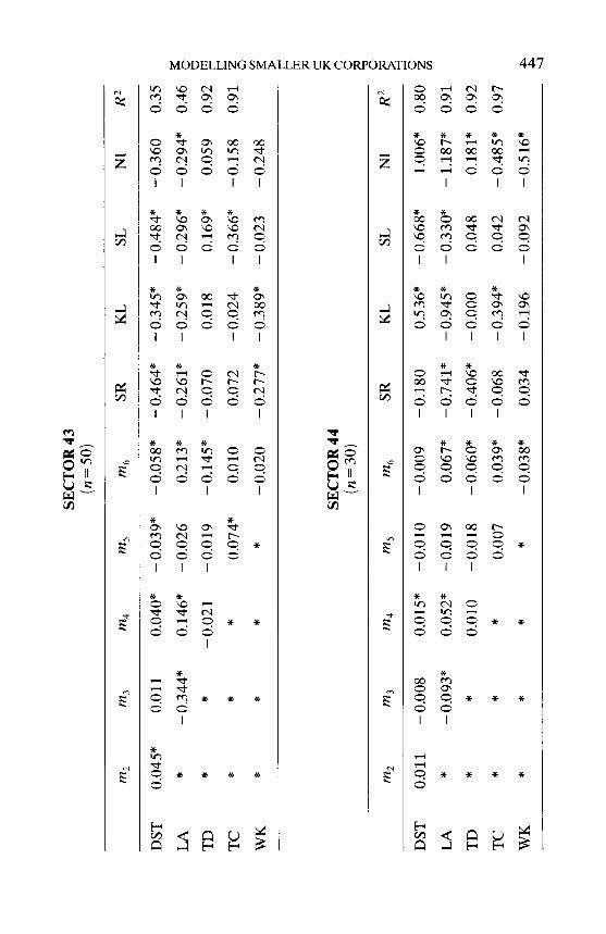
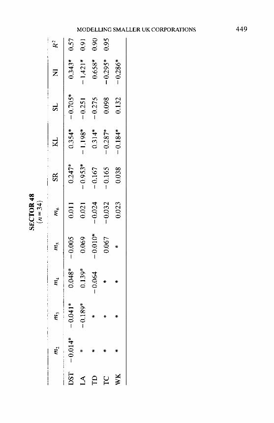
The full results of sectoral estimations are given in the Appendix: Table 3summarizes the signs and significance of the coefficients. For comparisonwith the six equation version we note the following characteristics of theresults:

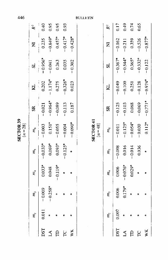
Thirty nine percent (76 out of 195) G matrix coefficients are significantat the 5 percent level. The restrictions of homogeneity and symmetry areaccepted in 8 out of the 13 sectors (see Table 1), confirming the finding withthe pooled version: note that with many G matrix coefficients significant, therestrictions are not easily accepted. These results give modest support for theparticular portfolio model developed in Section III.'°

Of the 65 G coefficients, 31 are positive (12 significant) and 34negative (15 significant). These negative G1 coefficients are contrary to theexpectations of the model. Inspection of the results suggests that there is aparticular problem with, m3, the cost of loan finance. In fact, m3, defined asbank base rate net of corporation tax relief and inflation, is negative for asubstantial part of the period under consideration. (The actual rate paid onbank borrowing would certainly have included a premium over base rate, butwe have not been able to find a suitable measure for this.) The economicimplication is that borrowing by firms must have been constrained byrationing rather than the cost of loans. The unexpected sign of the coefficientmay be picking up a supply of funds effect, with banks raising interest rateswhen firms needed to borrow more.

While the pattern of signs in the H matrix of coefficients (60 percentof which are significant) corresponds closely to that found with the pooledequation, it is evident that there is greater diversity in the G matrix, at leastfor some coefficients. For example, the coefficient on m4 in the pooledequation for trade debt (TD) is unequivocally positive and significant. But forthe sector equations the coefficient is evenly divided between positive andnegative values. Similarly, the coefficient on m4 in the pooled equation forloans (LA) is positive but not significant, but is significant in 5 of the sectors.

Courakis (1989) rightly emphasizes, the negative exponential utility function, fromwhich the model of Section III is derived is very specific. Rejection of symmetry and homo-geneity in five sectors may indicate that the model is inappropriate for those sectors. Insubsequent work, alternative specifications will be considered.

440 BULLETIN

(iv) A large number of firm dummies (55 percent) are significant, suggest-ing substantial interfirm variations, even within a sector.

(y) Lagrange multiplier tests indicated a problem with heteroscedasticityin just two sectors: Chemicals (26) and Metal Manufacture (31). These werethe two sectors where we were not able to choose firms of a similar size. Theabsence of heteroscedasticity in the majority of sectors gives greaterconfidence in the sectoral results, than for the pooled equation (for which theLagrange Multiplier statistics are large).

V. CONCLUSIONS

The econometric results reported in Section IV provide support for thefollowing conclusions:

(j) Firms' decisions about balance sheet items can be effectively modelledas a simultaneous system in which the effects of decisions about one elementof the balance sheet on other elements are explicitly accounted for.

The model in Section II is a particular example of how this interactionbetween balance sheet items may occur. Despite its specificity, many of itskey features are supported; the existence of symmetry and homogeneity, andthe role of non-choice items in forming a 'core' on which the portfolio ofassets and liabilities is built. In the five equation model the fact that nearly 40percent of the G matrix coefficients are significant is an indication thatportfolio effects are present. (The rejected null hypothesis is that these coef-ficients are zero, in which case the elements of the balance sheet are un-responsive to changes in relative returns and costs.) The least satisfactoryfeature of our results is the puzzling behaviour of some of the G.1 coefficients,but some of the difficulties may be attributable to our inability to find betterindicators for the relevant rates of return and costs for assets and liabilities.

The econometric performance of the model improved significantlywhen the net investment equation was dropped from the system, and netinvestment entered as a pre-determined variable. Our interpretation is thatnet investment is not determined simultaneously with the other items in thebalance sheet. Given lags in implementing investment decisions, theindependence of investment from more short-term decisions is unsurprising.(The alternative explanation for the weak performance of the investmentequation is simply that the measure of return to investment was inappro-priate.)

Pooling the data across sectors, while it generates acceptable results,conceals some differences in the G matrix coefficients between sectors. Whilesuch differences are not unexpected, given the differing characteristics ofsectors, it suggests that analysis based on pooled or even aggregate data maymislead.

We note that these results were obtained for a carefully chosen sample offirms with homogeneity of size within sectors, a fairly stable history, andrelatively small average size within the whole quoted sector. The same model


does not work well with a sample of large corporations where managerialgrowth objectives are thought to be more prominent.'1 In previous work onunquoted firms (Hay and Louri, 1989) using a similar portfolio model, it wasnot necessary to drop the net investment equation to get satisfactory results,implying greater interaction between the long-term and short-term decisionsof the firm. The comparison strengthens the suggestion noted above thatbehaviour varies between firms, and that aggregate analysis may mislead.

Jesus College, OxfordAthens University of Economics & Business

Date of Receipt of Final Manuscript: June 1991

REFERENCES

Bosworth, B. (1971). 'Patterns of Corporate External Financing', Brookings Papers inEconomic Activity, Vol. 2, pp. 253-84.

Blinder, A. S. and Maccini, L. (1991). 'Taking Stock: A Critical Assessment of RecentResearch on Inventories', Journal of Economic Perspectives, Vol. 5, pp. 73-96.

Brainard, W. C. and Tobin, J. (1968). 'Pitfalls in Financial Model Building', AmericanEconomic Review, Vol. 58, pp. 99-122.

Chowdhury, G., Green, C. J. and Miles, D. K. (1986). 'An Empirical Model ofCompany Short-Term Financial Decisions: Evidence from Company AccountsData', Bank of England Discussion Paper, No. 26.

Courakis, A. S. (1974). 'Clearing Bank Asset Choice Behaviour: A Mean-VarianceTreatment', BULLETIN, Vol. 36, pp. 173-202.

Courakis, A. S. (1975). 'Testing Theories of Discount House Portfolio Selection',Review of Economic Studies, Vol. 42, pp. 643-48.

Courakis, A. S. (1980). 'In Search of an Explanation of Commercial Bank Short-RunPortfolio Selection', BULLETIN, Vol. 42, pp. 305-36.

Courakis, A. S. (1988). 'Modelling Portfolio Selection', Economic Journal, Vol. 98,pp.619-42.

Courakis, A. S. (1989). 'Does Constant Relative Risk Aversion Imply Asset Demandsthat are Linear in Expected Returns?', Oxford Economic Papers, Vol. 41, pp.553-66.

Croasdale, M. (1988). 'Modelling the Finance of Investment', Chapter 10 in Harris,L., Coakely, J., Croasdale, M. and Evans, T., New Perspectives on the FinancialSystem, Croom Helm, London.

Dhrymes, P. J. and Kurz, M. (1967). 'Investment, Dividend and External FinanceBehaviour of Firms', in Ferber, R. (ed.), Deter,ninants of In vestment Behaviour,NBER, New York, pp. 427-67.

Duncan, G. M. (1983). 'Estimation and Inference for Heteroscedastic Systems ofEquations', International Economic Review, Vol. 24, pp. 5 59-66.

We plan further research to find an empirical model for the balance sheet behaviour oflarge corporations. We also hope to look at the determinants of intersectoral and interfirmdifferences in balance sheets.

442 BULLETIN

Edwards, J. S. S., Kay, J. A. and Mayer, C. P. (1987). The Economic Analysis ofAccounting and Profitability, Oxford University Press, Oxford.

Friedman, B. (1979). 'Substitution and Expectation Effects on Long-term BorrowingBehaviour and Long-term Interest Rates', Journal of Money, Credit and Banking,Vol. ll,pp. 131-50.

Goudic, A. W., Meeks, G., Wheeler, J. M. and Whittington, G. (1985). 'The Cam-bridge/DTI Databank of Company Accounts: An Introduction for Users'mimeo, Department of Applied Economics, Cambridge, UK.

Grabowski, H. G. and Mueller, D. C. (1972). 'Managerial and Stockholder WelfareModels of Firm Expenditures', Review of Economics and Statistics, Vol. 54, pp.9-24.

Hay, D. A. and Lour, H. (1989). 'Firms as Portfolios: A Mean-Variance Analysis ofUnquoted UK Companies', Journal of Industrial Economics, Vol. 38, pp. 14 1-65.

Hay, D. A. and Morris, D. J. (1984). Unquoted Companies: Their Contribution to theUK Economy, Macmillan, London.

Hay, D. A. and Morris, D. J. (1991). Industrial Economics and Organisation: Theoryand Evidence, Oxford University Press, Oxford.

Jackson, P. D. (1984). 'Financial Asset Portfolio Allocation of Industrial andCommercial Companies', Bank of England Discussion Paper (Technical series), No.8.

Kay, J. A. and King, M. A. (1986). The British Tax System, Oxford University Press,Oxford.

Mueller, D. C. (1967). 'The Firm Decision Process: An Econometric Investigation',Quarterly Journal of Economics, Vol. 83, pp.58-87.

Parkin, J. M. (1970), 'Discount House Portfolio and Debt Selection Behaviour',Review of Economic Studies, Vol. 37, pp. 469-97.

Parkin, J. M., Gray, M. R. and Barrett, R. J. (1970). 'The Portfolio Behaviour ofCommercial Banks', in Hilton, K. (cd.), The Econometric Study of the UnitedKingdom, Macmillan, London, pp.229-51.

Sharpe, 1. (1973). A Quarterly Econometric Model of Portfolio Choice', TheEconomic Record, Vol. 49, pp. 518-33.

Taggart, R. A. (1977). A Model of Corporate Financing Decisions', Journal ofFinance, Vol. 32, pp. 1467-84.

Valentine, I. J. (1973). 'The Demand for Very Liquid Assets in Australia', AustralianEconomic Papers, Vol. 12, pp. 196-207.

APPENDIX: FIVE EQUATION VERSION OF MODEL: RESULTS BY SECTOR

Notes:An asterisk by a reported coefficient indicates that it is statistically significant at at least

the 5 percent level.n = number of observations.

SEC

TO

R 2

1(n

=33

)

t-

m3

m5

nl6

SRK

LSL

NI

R2

DST

0.05

2*0.

029

-0.0

11-0

.020

-0.0

50-0

.012

0.03

6_0

.729

*0.

287*

0.44

*-0

.086

0.06

6-0

.049

0.04

0_0

.430

*_0

.533

*-0

.029

_0.3

01*

0.86

TD

**

-0.0

110.

057

_0.1

00*

-0.1

060.

055

0.27

3-0

.035

0.88

TC

**

*0.

002

0.01

00.

011

_0.1

95*

0.27

9_0

.526

*0.

89

WK

**

**

0.10

0_0

.456

*_0

.364

*_0

.794

*-0

.425

SEC

TO

R 2

3(n

=39

)

m2

m4

SRK

LSL

NI

R2

DST

-0.0

160.

014

0.04

7*-0

.002

_0.0

44*

0.08

80.

133

_0.4

08*

0.16

50.

28

JJ*

-0.1

030.

009

-0.0

170.

097

_0.7

58*

_0.7

93*

-0.6

71_0

.972

*0.

80

TD

**

-0.0

230.

023

-0.0

49_0

.204

*-0

.105

0.41

7*0.

249*

0.80

TC

**

*_0

.079

*0.

075*

-0.0

61-0

.100

_0.3

50*

_0.2

60*

0.74

WK

**

**

-0.0

79-0

.065

_0.1

35*

0.01

1_0

.181

*

SEC

TO

R 2

6(n

=63

)-

m2

m3

m6

SRK

LSL

NI

R2

DST

0.07

5*

-0.0

390.

173*

-0.0

71_0

.137

*_0

.243

*_0

.122

*-0

.393

*0.

164*

0.33

TD

*

- 1.

693*

*

0.83

4*-0

.111

1.00

9*_0

.222

*_0

.286

*0.

319*

_0.4

71*

0.56

TC

*

0.01

0_0

.374

*_0

.644

*_0

.297

*-0

.146

0.46

0*0.

356*

0.92

*

**

-0.0

150.

571*

0.11

00.

046

_0.6

64*

_0.5

04*

0.91

WK

**

*_0

.801

*_0

.348

*_0

.491

*-0

.084

-0.5

45*

SEC

TO

R 3

1(n

=67

)

in2

in3

in4

in5

in6

SRK

LSL

NI

R2

DST

0.02

5*

-0.0

340.

091*

-0.0

940.

012

0.00

40.

053

_0.4

25*

-0.0

610.

33

TD

*

-0.2

24-0

.289

0.32

5*0.

221

0.07

2*_0

.096

*0.

024

_0.3

37*

0.83

TC

*

* *

0.47

4*-0

.183

-0.0

92_0

.183

*-0

.054

0.50

8*0.

044

0.93

WK

*

*-0

.372

0.32

4*_0

.271

*_0

.391

*_1

.146

*_0

.376

*0.

85*

**

_0.4

64*

_0.4

78*

_0.5

12*

0.04

0_0

.271

*

SEC

TO

R 3

3(n

69)

SEC

TO

R 3

6(n

44)

m2

m4

m6

SRK

LSL

NI

R2

DST

0.02

7*0.

002

-0.0

02-0

.002

-0.0

23_0

.138

*0.

037

_0.6

08*

0.24

70.

33*

-0.0

150.

005

-0.0

120.

019

-0.0

230.

023

0.03

50.

021

0.17

TD

**

0.07

4*-0

.022

_0.0

55*

0.02

50.

308*

0.06

10.

226

0.74

TC

**

*-0

.031

0.06

7*_0

.069

*0.

163*

-0.0

56-0

.021

0.74

WK

**

**

-0.0

05_0

.796

*_1

.159

*_0

.432

*_1

.473

*

m2

m3

m4

m5

m5

SRK

LSL

NI

R2

DST

0.06

9-0

.005

0.06

40.

047

_O.1

75*

-0.0

210.

053

_0.1

25*

0.22

6*0.

27*

-0.4

920.

391*

_0.4

16*

0.52

4*_0

.311

*_Ø

399*

_0.4

62*

_Ø74

9*0.

88

TD

**

_0.2

71*

0.43

6*_0

.620

*-0

.062

0.06

70.

296*

0.23

2*0.

41

TC

**

*_0

.712

*0.

645*

_0.2

88*

_0.3

63*

0.63

3*_O

.601

*0.

92

WK

**

**

-0.3

75_O

.318

*_0

.358

*-0

.076

-0.1

07

SEC

TO

R 3

9(n

28)

m3

m4

m5

m6

SRK

LSL

NI

R2

DST

0.01

1-0

.009

0.03

3*_0

.033

*-0

.003

-0.0

210.

202

_0.9

56*

0.23

50.

40*

_0.2

58*

0.04

80.

069*

0.15

1*_0

.964

*-

1.17

4*-0

.041

_0.8

49*

0.95

TD

**

_0.1

19*

0.09

3*-0

.055

-0.0

890.

275

0.26

30.

457*

0.95

TC

**

*_0

.125

*-0

.004

-0.1

13_0

.326

*0.

035

_0.4

17*

0.93

WK

**

**

_0.0

90*

0.18

70.

023

-0.3

02_0

.428

*

SEC

TO

R 4

1(n

= 4

8)

m2

m3

m4

m5

m6

SRK

LSL

NI

R2

DST

0.00

70.

006

0.00

6-0

.008

-0.0

11-0

.125

-0.0

49_0

.367

*-0

.162

0.17

LA

*0.

179*

_0.0

76*

0.01

6_0

.125

*-0

.103

-0.1

00_0

.544

*-0

.211

0.49

TD

**

0.02

9*-0

.014

_0.0

54*

0.06

80.

251

0.36

5*0.

359

0.74

TC

**

*0.

036

-0.0

30-0

.069

-0.1

28_0

.332

*-0

.526

0.65

WK

**

**

0.11

2*_0

.771

*_0

.974

*-0

.122

_0.8

77*

SEC

TO

R 4

3(n

50)

m2

m4

m5

m6

SRK

LSL

NI

R2

DST

0.04

5*0.

011

0.04

0*_0

.039

*_0

.058

*O

.464

*0.

345*

0.48

4*-0

.360

0.35

LA

*_0

.344

*0.

146*

-0.0

260.

213*

_0.2

61*

_0.2

59*

_0.2

96*

_0.2

94*

0.46

oT

D*

*-0

.021

-0.0

19_0

.145

*-0

.070

0.01

80.

169*

0.05

90.

92rî

i

TC

**

*0.

074*

0.01

00.

072

-0.0

24_0

.366

*-0

.158

0.91

z C)

WK

**

**

-0.0

20_0

.277

*_0

.389

*-0

.023

-0.2

48r-

SEC

TO

R 4

4(n

30)

o

m2

m3

m5

SRK

LSL

NI

R2

DST

0.01

1-0

.008

0.01

5*-0

.010

-0.0

09-0

.180

0.53

6*_0

.668

*1.

006*

0.80

*_0

.093

*0.

052*

-0.0

190.

067*

_0.7

41*

_0.9

45*

_0.3

30*

_1.1

87*

0.91

TD

**

0.01

0-0

.018

_0.0

60*

_0.4

06*

-0.0

000.

048

0.18

1*0.

92

TC

**

*0.

007

0.03

9*-0

.068

_0.3

94*

0.04

2_0

.485

*0.

97

WK

**

**

_0.0

38*

0.03

4-0

.196

-0.0

92_0

.516

*

SEC

TO

R 4

6(n

35)

m3

m5

m6

SRK

LSL

NI

R2

DST

0.42

3*-0

.166

0.72

4*_0

.510

*-

0.47

1*_0

.123

*-0

.042

-0.5

87*

0.02

90.

49

LA

*1.

400

-0.8

19

-0.5

660.

15 1

- 0.

338*

- 0.

353*

0.08

0-

0.72

7*0.

87

TD

**

2.06

4*-0

.5 7

0*-0

.399

-0.0

26-0

.008

- 0.

525*

- 0.

421*

0.96

TC

**

*2.

644*

0.00

2-

0.08

5*-

0.32

1*0.

207*

- 0.

396*

0.91

WK

**

*0.

717

- 0.

481*

- 0.

275*

-0.1

72-

0.32

7*

SEC

TO

R 4

7(n

=48

)

m2

m3

m5

m6

SRK

LSL

NI

R2

DST

0.06

2_0

.018

*0.

013

-0.0

03-0

.061

0.12

1*-

0.74

8*0.

170

0.45

LA

*_0

.153

*0.

033

0.04

80.

092*

- 0.

479*

_0.4

45*

0.13

7-0

.6 5

7*0.

69

TD

*-

0.02

90.

028

- 0.

045

- 0.

422*

-0.1

16-0

.013

0.20

50.

80

TC

**

0.01

8-

0.09

6*0.

344*

_0.1

42*

-0.0

05-

0.20

8*0.

91

WK

**

0.05

2_0

.382

*_0

.418

*-

0.37

5*_0

.510

*

SEC

TO

R 4

8(n

34)

rn,

m3

m4

m5

rn6

SRK

LSL

NI

R2

DST

_0.0

14*

_0.0

41*

0.04

8*-0

.005

0.01

10.

247*

0.35

4*_0

.705

*0.

343*

0.57

*_0

.189

*0.

139*

0.06

90.

021

_0.9

53*

_1.1

98*

-0.2

51_1

.421

*0.

91

TD

**

-0.0

64_0

.010

*-0

.024

-0.1

670.

314*

-0.2

750.

658*

0.90

TC

**

*0.

067

-0.0

32-0

.165

_0.2

87*

0.09

8_0

.295

*0.

95

WK

**

**

0.02

30.

038

_0.1

84*

0.13

2_0

.286

*

Documents

MODELLING SMALLER UK CORPORATIONS: A PORTFOLIO ANALYSIS