Modelling meteorological and substrate influences on peatlandhydraulic gradient reversais

Dennis ColauttiDepartment ofGeography

McGill UniversityMontréal, Québec

August 2001

A thesis submitted ta the Faculty ofGraduate Studies and Research inpartial fulfillment ofthe requirements ofthe degree ofMasters of

Science

© Dennis Colautti 2001

1+1 National Libraryof Canada

Acquisitions andBibliographie Services

395 Wellington StreetOttawa ON K1A ON4canada

Bibliothèque nationaledu Canada

Acquisitions etservices bibliographiques

395. rue WellingtonOttawa ON K1 A ON4canada

Your liIe VOIle rflf#j_

The author has granted a non­exclusive licence allowing theNational Library ofCanada toreproduce, loan, distribute or sellcopies of this thesis in microform,paper or electronic formats.

The author retains ownership ofthecopyright in this thesis. Neither thethesis nor substantial extracts from itmay be printed or otherwisereproduced without the author'spemnsslon.

L'auteur a accordé une licence nonexclusive permettant à laBibliothèque nationale du Canada dereproduire, prêter, distribuer ouvendre des copies de cette thèse sousla forme de microfiche/film, dereproduction sur papier ou sur formatélectronique.

L'auteur conserve la propriété dudroit d'auteur qui protège cette thèse.Ni la thèse ni des extraits substantielsde celle-ci ne doivent être imprimésou autrement reproduits sans sonautorisation.

0-612-78851-2

Canada

Table of Contents

ABSTRACT 1

RÉSUMÉ 11

ACKNOWLEDGEMENTS III

LIST OF FIGURES IV

LIST OF TABLES IV

CHAPTER 1.0 INTRODUCT10N l

CHAPTER 2.0 LITERATURE REVIEW AND RESEARCH OBJECTIVES 2

2.1 GENERAL INTRODUCTION TD PEATLAND HYDROLOGY AND GROUNDWATER MODELLlNG 32.1.1 Peatlands and their hydrology 32.1.2 Contemporary numerical modelling and ils application to peatlalld subsurface flow.........................................................................................................................................102.13 Contemporary studies ofsubsurjace flow reversais in peatlands 14

2.2 RESEARCH OBJECTfVES 19

CHAPTER 3.0 RESEARCH METHODOLOGY 20

3.1 MODELDOt'vlAfN DESCRIPTIONS 213.2 MODEL METEOROWGICAL FORCING AND SUBSTRATE ALTERATION 223.3 MODELRUNCONFlGURATlONS 24

CIIAPTER 4.0 RESULTS 25

4.1 [.RET SIMULATIONS 264.1.1 F~treme drought conditions 264.1.2 Drought severity variatwll .324.13 Catotell'll aUeration ; .414.1.4 Discussion ofLRET simulations ..42

4.2 KBT SIA.fULATlONS 474.2.1 Extreme drougllt conditions .474.2.2 Hydraulic conductivity .484.2.3 Drough.t severity variation 494.2.4 Porosity 504.2.5 Discussion ofKET sùnulations 51

CHAPTER 5.0 SUMMARY AND CONCLUSION : 54

REFERENCES 57

Abstract

A hydrological modelling effort using MODFLOW wasundertaken in order ta determine the relative importance ofsorne of the factors influencing hydraulic gradient reversaIs inpeatlands. Model domains were of two types, large raised bogtype (LRBT) and kettle bog type (KBT), and were made toundergo various levels of meteorological forcing (waterdeficit). Substrate, too, was varied in order to determine itsimportance on reversaIs. Domain-wide reversaIs weresuccessfully sitnulated in LRBT systems, but not in KBTsystems. Although simulated flow patterns matched fieId­observed patterns, both pre- and post- drought, simulatedreversaIs occurred more quickly than in the field. This Inay bedue to insufficientIy distributed parameters, such as hydraulicconductivity. ReversaIs were easily terminated by simulatingnon-drought conditions. In the LRBT system, reversaI durationdecreased, and time-to-reversal increased, with a decrease indrought severity. Increasing drought severity in KBT systemshad the opposite effect on the duration of semi-reversed flowpatterns, suggesting a possibly different/additionalmechanism for flow reversaIs in KET systems. Hydraulicconductivity had an appreciable effect on flow reversaIevolution, though neither changing porosity, nor differencesin catotelm Iayering had a great effect.

i

Résumé

Une étude hydrologique a été effectuée, en utilisant le logicielMODFLOW, afin de déterminer l'importance relative descertains des facteurs qui peuvent influencer les renversementsde gradient hydraulique dans deux types fondamentaux (LRBTet KBT) de tourbière. Les deux types ont été subis à dediverses conditions météorologiques (déficit d'eau). Aussivarié était le substrat, afin de déterminer son importance. Desrenversements ont été fructueusement simulés partout dansles systèmes LBRT, mais pas dans les systèmes KBT. Bien queles simulations de flux ressemblaient, en forme, desrenversements observés, les renversements simuléesurvenaient beaucoup plus vite que dans la nature, peut être àcause de l'utilisation des paramètres insuffisammentdistribués, tel conductivité hydraulique. Les renversementsétaient terminés aisément avec la simulation des conditions denon-sécheresse. La durée de renversement diminuait, et letemps requis pour effectuer le renversement accroissait, avecune diminution dans la sévérité de sécheresse dans lessystemes LRBT. Inopinément, la durée des semi-renversementsdans les systemes KBT diminuait avec les plus grandessécheresses. Ceci suggére un mécanisme alternative/différentpour effectuer des renversements dans les systèmes KBT.Quant à l'évolution des renversements, conductivitéhydraulique était plus important que les différences dans lesconfigurations variables de catotelm et aussi la porosité.

ii

Acknowledgements

1 thank Nigel Roulet for his supervision, advice, and

patience -- especially the patience.

Financial assistance was provided by a NSERC PGS-A (two­

year postgraduate scholarship).

Support from family and friends back home was invaluable,

and 1am very grateful for having received it.

Hi

List of Figures

4.1.1 Selected time steps of Simulation 4.1.14.1.2 Selected time steps of Simulation 4.1.24.1.3 Selected time steps of Simulation 4.1.34.1.4 Selected time steps of Simulation 4.1.44.1.5 Selected time steps of Simulation 4.1.54.1.6 Selected time steps of Simulation 4.1.64.1.7 Selected time steps of Simulation 4.1.74.1.8 Selected time steps of Simulation 4.1.84.2.1 Selected Ume steps of Simulation 4.2.14.2.2 Selected time steps of Simulation 4.2.24.2.3 Selected time steps of Simulation 4.2.34.2.4 Selected time steps of Simulation 4.2.5

List of Tables

4.1 LRBT configurations and parameters4.2 LRBT surface boundary conditions4.3 KBT configurations and parameters4.4 KBT surface boundary conditions

iv

Chapter 1.0 Introduction

Over the past few years, a peculiar peatland groundwater

flow phenomenon has been observed in the field, with possible

consequences for peatland biota on the local scale, and, on a

much larger scale, for global dimate change. The

phenomenon in question involves the periodic reversaI of the

usual hydraulic gradients within an unconfined aquifer of

certain peatlands, which reverses the usual groundwater flow

direction. Because such reversaIs have been observed

particularly after the onset of periods of water deficit, it has

been hypothesized that they result from a time lag in pressure

transmission down the peat column, due, in turn, ta the law

hydraulic conductivity of peat.

The aim of the present study is ta numerically madel

variaus peatland settings in arder to elucidate haw various

levels of drought influence the short-term evolution of

gradient reversaIs, and how the peat substrate itself might

influence said evalutian. The appraach taken is not one in

1

which real-world peatlands are modelled exaetly. Instead, the

simulations contained herein are the resuit of generai

parameter input, since the goal is to bring to light the relative

effects that various forcing agents (meteorology, substrate

characteristics) have on the development of hydraulic

gradient reversaIs, which may give insight into other

phenomena, such as peatland vegetation change and methane

outgasing.

Chapter 2.0 Literature review and research

objectives

This purpose of this chapter is three-fold: (1) to introduce

peatlands, general peatiand hydrology (peatland subsurface

flow reversaIs in particular), and the more salient aspects of

groundwater modelling to the reader; (2) to discuss flow

reversaIs, a specifie aspect of peatland hydrology, in the

eontext of the relevant scientific literature; and (3) to outline

the modelling objectives as they relate to groundwater flow

2

reversaIs in several differing hypothetical peatland (bog)

settings.

2.1 General introduction to peatland hydrology

and groundwater modelling

2.1.1 Peatlands and their hydrology

Hydrology plays a leading role in peatland development,

chemistry, and biology (Glaser et al., 1981: Mitsch and

Gosselink, 1993; Waddington and Roulet, 1997). A good

understanding of peatlands, therefore, relies on a good

understanding of peatland hydrology, but before focussing on

some of the specifies of peatland hydrology, a distinction

between the different types of peatlands is usefuI.

In general, two basi€ types of peatlands exist: fens and

bogs (Glaser et al., 1981; Ingram, 1983). Fens tend to have fiat

or concave surfaces which are not higher than the

surrounding landscape. Bogs, however, tend to have a higher

surface than their surroundings, and very often are domed.

3

Fen waters are characterized by pH values greater than 4.2

and by concentrations of inorganic solutes which are higher

than those of bogs (e.g., fen calcium concentrations typically

are greater than 2.0 ppm, while bog concentrations typically

are lower than 2.0 ppm); bog waters typically have pH values

lower than 4.2 (Reeve et a1., 2000). Because the type of

vegetation growing in a particular wetland depends on surface

water chemistry, it is not surprising, then, that the biota of

fens and bogs differs significantly, with the former typically

being dominated by calciphilic flora -- especially sedges, such

as the Carex species -- and the latter by mosses, such as the

Sphagnum species.

The aforementioned morphology, biology, and chemistry of

peatlands have led many researchers to make certain

inferences about the origin of water that sustains these

landforms. For instance, it is thought that differences in

chemistry result from fens being supplied, in large part, by

groundwater (i. e., water flowing upwards into the fen,

through underlying mineraI sediments, and derived possibly

from regional groundwater flow) , and from bogs being

4

supplied almost exclusively by direct meteoric (Le., solute­

poor) water input. This, in turn, is thought to arise largely

from the difference in landform morphology between these

two peatland types. That is, because bogs tend to have convex

surfaces, water table mounds form under their surface, and

this leads to almost exclusively recharge conditions. This is

thought to prevent sub-bog groundwater from discharging

into the bog; thus, mineral-poor, directly-derived meteoric

water constitutes, by far, most of the bog's water supply.

Contrastingly, the concave surface of a fen is thought to lead

to recharge conditions which are so strong that they prevent

sub-fen, mineral-rich groundwater from discharging into the

fen.

Further to the differences between the two basic types of

peatlands, there are many different types of bogs. Two are

studied in this thesis: the blanket bog, and the kettle bog.

The differences between these two types arise from their

topographie setting. The blanket type is characterized by a

gently sloping surface everywhere except for the steeply

sloping margins. AIso, blanket bogs are much more expansive

5

than are kettle bogs, and often are underlain by a rather

impermeable, fiat mineraI substrate layer. Their greater areal

expanse is due to their ability to expand laterally over rather

fiat terrain. Kettle bogs, on the other hand, form in

depressions often left behind by glacial activity, and thus are

characterized by a rather pronounced concave lower

boundary. Their upper surfaces often are domed, and slope

gently from their central regions up to and including their

margins. The margins coincide approximately with the rim of

the depression, which greatly confines lateral expansion of the

kettle bog. Thus, the blanket bog is able to grow in more of a

horizontal manner, whereas the kettle bog has to grow in a

more vertical manner. In the case of both types, there often is

a water conduit, or 'lag', found at the bog margin, which

serves to drain and channel water away from the bog. Also

common to both bog types is the presence of two distinct peat

layers -- the acrotelm and the catotelm (Ingram, 1983). The

former term refers to the uppermost peat layer, which often is

about 50 cm in thickness (e.g., Devito et aL, 1997; Fraser,

1999), is composed mainly of living plants and slightly

6

decomposed peat, and thus is characterized by hydraulic

conductivity (K) values of about 10-2 ms-! (Ivanov, 1981; Roag

and Priee, 1995). The underlying catotelm, which rests

directly on the mineraI substrate, is composed of much more

humified peat, and thus has a much lower overaIl K value of

about 10-5 ms-! to 10-8 ms-! (Chason and Siegel, 1986). Because

of this, many (Ingram, 1983; Ingram and Bragg, 1984, for

example) have hypothesized that the acrotelm may channel

water quickly to the margins' lags, while the catotelm may be

relatively inactive with respect to groundwater flow, and may

not even interact significantly with the underlying, mineraI

substrate. The assumption that most of the drainage of bogs is

effected by only a thin (-50 cm) surface layer is one reason

that deeper bog peat has not been studied to the extent that

the more superficial bog peat has been studied.

Whether or not deeper bog peat plays a significant role in

bog drainage, we can point to sorne general groundwater flow

features of peat bogs. For instance, flow in bogs is said to be

Darcian, as opPOsed to laminar, in nature (Hemond and

Goldman, 1985). Renee, the general continuity equation,

7

based on Darcy's Law, may be used ta describe saturated

subsurface flow in bag settings:

(1)

where: Kx, Ky, and ~ are camponents of the hydraulic

conductivity tensor; h is hydraulic head; S5 is specifie storage;

W is a general sink/source term, and where the three spatial

dimensions are represented by x, y, and z (Freeze and Cherry,

1979).

Another general feature of bog subsurface flow is the

steepening of hydraulic gradients as one goes from a bog's

centre to its margins (Ingram, 1982; Gafni and Brooks, 1990),

and yet another is the general tendency for subsurface water

to flow from a bog's centre, downwards to sorne extent, and

outwards to its margins. However, of increasing interest, due

to its contradiction of the last-l'downwards and outwards" flow

feature, is the field-observed phenomenon of groundwater

flow reversaIs in bogs (Fraser, 1999; Devito et al., 1997;

8

Romanowicz et al., 1993). This phenomenon has been

obsetved to occur soon after the onset of significant drought

conditions. It is thought to arise from a time lag in the vertical

transmission of hydraulic pressure change as water is

removed, by the drought, from the uppermost region of the

peat column. That is, the near-surface pressure is thought to

change rapidly in response to the removal of near-surface

water, while deeper peat water experiences the drought­

induced pressure change much later. This time lag is thought

to come about due to the very low hydraulic conductivity

values of peat -- especially deeper peat, which almost always is

orders of magnitude less conductive than is the acrotelm's

peat. Until the deeper peat water undergoes a pressure

decrease, the water pressure in the vicinity of the water table

(where water is being removed from the system) may

temporarily drop below that of deeper peat water, thus

effecting flow more upwards than usual (Fraser, 1999).

9

2.1.2 Contemporary numerical modelling

and its application to peatland subsurface

flow

In view of the important effects that hydrology has on

various peatiand processes, it is not surprising that there have

been many studies of peatland hydrology. The complexity of

peatland systems, as is the case with many non-peatland

groundwater systems, makes the numerical modeUing

approach especially attractive. For instance, the present

study, which seeks to elucidate the importance of various

hydrogeologicai factors in bog groundwater flow reversaIs,

does so by varying a single factor (e.g., precipitation level)

from one numerical simulation to the next, with aU factors

remaining equal. It would be impossible to find real-world

bogs which varied (which could he controlled) in such a

fashion. Unfortunately, only a few studies to date (Reeve et

al., 2000; McNamara et al.,1992; McKenzie, 1997; Siegel, 1981,

1983) have made use of the numerical modeUing approach in

studying peatland subsurface water flow. McNamara et al.

10

(1992) modelled the linked evolution of peatiand morphology

and hydrology, while McKenzie (1997) modelled this and

varying hydrogeological configurations' effects on peatland

groundwater flow. McNamara et aI. (1992) observed a

permanent reversaI in flow during the fen-to-bog evolution

which was the focus of their study. They credit the slightly

minerotrophic nature of their study bog vegetation to periodic

reversaIs of hydraulic gradients, which result in the discharge

of mineral-rich groundwater to the bog. However, both of

these studies focused on long-term peatland hydrology

change, thus negiecting changes of a temporary nature,

including temporary flow reversaIs, which have been observed

in field studies.

Much more modelling has been done for the non-peatland

setting, beginning with Toth (1963) and Freeze and

Witherspoon (1967) who investigated the effects of various

hypothetical hydrogeological configurations on generailocal­

to-regional-scale groundwater flow in small basins. Winter

(1978) and Cheng and Anderson (1994) did the same with

respect to lake/groundwater systems. Anderson and Munter

Il

(1981) looked at the effects of various configurations on

groundwater flow reversaIs around lakes. But, contrary to

Ingram's (1991) assertion that bogs are virtually lakes, they

are essentially mounds of water, with Uttle solid matter and

therefore are characterized by internaI hydraulic gradients.

Because of these bog-Iake differences and the lack of

modelling studies with respect to short-term, transient

hydrologicai change in bogs, there is a need to model the

occurrence, frequency, and magnitude of groundwater of flow

reversaIs within bogs (see next section for introduction to flow

reversaIs) .

Briefly, numerical modelling involves discretizing of a

domain (the bog, in the present study) into cells, in one, two,

or three dimensions, and assigning equations (see Equation 1)

to each individual cel!. Here, the solution of each cell's

equation results in a hydraulic head value, which is assigned

to the appropriate cell. From the pattern of hydraulic head

values , one may determine how groundwater flows

throughout the modelled domain. As with any such modeI,

the validity of the results is highly dependent upon the

12

validity of the input data and the numerical scheme used.

Thus, while the present study presents numerous flow

patterns, it should not be forgotten that these patterns are

dependent upon input data sets which are incomplete. For

example, within a bog, hydraulic conductivity is highly

variable even within distances of a few centimeters (Fraser,

1999). Because of this, it is impossible to sample every single

Kvalue within a peatland without destroying the system,

which in turn makes it impossible to create a numerical model

which is completely accurate in its description of a bog in

terms of K. The same can be said about describing the bog's

lower boundary condition, or about porosity or storativity

values. Hence, it becomes necessary to extrapolate the values

that we do have; we do no discretize a bog dOlnain in such a

wayas to account for every real-world Kvalue. Instead, a

single K value may be assigned to a cell covering tens of

meters spatially (as opposed to a few centimeters), and bog

boundaries are made to be smooth and symmetrical. Of

course, this isn't the case in the field, but in the present study

the purpose is not to exactly replicate real-world bogs; instead,

13

the approach is ta simulate bogs to an extent which allows us

to make very general conclusions about how their subsurface

flow patterns might react in response to changes in forcing

conditions -- especially drought severity.

2.1.3 Contemporary studies of subsurface

flow reversaIs in peatIallds

Siegel (1988) investigated the recharge-discharge function

of Alaskan wetlands -- a function used to determine the

importance of wetlands to the environment. Recharge

wetlands contribute a certain proportion of their groundwater

to underlying mineraI sediments via downward flow, thus

possibly helping to repienish aquifers. Discharge wetlands

receive upward-moving groundwater from underlying mineraI

sediments, which can keep water tables high and import

nutrients to these wetlands, thereby affecting their ecology.

However, McNamara et. al. (1992) point out that the above

delineations are merely the results of inductive Inference .

Periodic reversaIs in hydraulic gradient and, thus, in

14

groundwater flow direction have been observed in the field

(Fraser, 1999; Devito et al., 1997; Romanowicz et al., 1993),

illustrating that sorne wetlands are recharged at certain times,

and discharge groundwater at other times. Thus, a particular

bog may not necessarily faIl into the recharge categoI}' on a

permanent basis. Wetlands such as bogs that are thought by

many ta be removed from intermediate and regional flow

systems may receive upwelling, possibly nutrient-Iaden

groundwater from these sub-systems (or at least from

groundwater system(s) beyond the bog perimeter) from Ume

ta time, thus having important effects on wetland chemistI}'

and biota. Furthermore, such upwelling can play an important

role in the pattern of release of greenhouse gases such as

methane (Romanowicz et al., 1993).

More recently, Fraser (1999) observed a reversaI in

subsurface bog water flow at Mer Bleue in 1998 -- a blanket

bog situated near Ottawa, Canada. Throughout the period

from mid-July ta roughly the end of August, water table draw­

down occurred, due to evapotranspiration greatly exceeding

precipitation. As the bog's water table elevation decreased by

15

up ta 20 cm, the head values of deeper peat water decreased

by only 10 cm. Since the difference in hydraulic head from

the surface to the base of the peatland was less than 10 cm, a

situation arose where the levels at depth were greater than

those at the surface. The head values of deeper peat water did

gradually decrease, approaching those of surface head values,

but only after six weeks. The flow reversaI came to an end

when the water table elevation increased due to a rainfall at

the end of August, 1998. The surface head values became

higher than those at depth, and the bog's 'normal' recharge

condition was restored. Although the storm caused deeper

head values to increase marginally, surface values increased

by much more. Fraser attributed his flow reversaI to drought

which was driven in large part by measured

evapotranspiration. He discounted the possibility of regional

flow since Mer Bleue is isolated from regional flow by means of

an underlying, low-K stratum.

Devito et al. (1997) came to a similar conclusion: intra-bog

flow reversaIs can occur even when the bog is isolated from

regional flow; and such reversaIs may arise due to the onset of

16

water deficit. These researchers observed such behaviour in

two bogs in Ontario, Canada, and in one bog in Sweden. AlI

three bogs were isolated from any groundwater flow beyond

their perimeters and bases. Upward flow was observed after

the onset of drought, leading the researchers ta conclude that

groundwater forcing from outside the bog proper is not at aH

necessary ta effect flow reversaIs. At the Dorset bog (southem

Ontario), usual downward flow changed ta upward flow (2

mm/day) in response to the water table dropping to 60 cm

below the peat surface). At the other Canadian site

(Experimental Lakes Area, northwestern Ontario), a water table

drop ta 20 cm below the average elevation resulted in a

change of flow from the usual 9 mm/day to the reversed DA

mm/day. Similarly, the Swedish bog (northern Sweden, near

Umeà), after experiencing a water table drop of greater than

15 cm, displayed a discharge pattern, which ended with a

precipitation event. These authors go so far as to state that

bogs typical of Canada's Precambrian Shield region (Le., bogs

which experience ephemeral groundwater input due to their

being disconnected from non-local sources of groundwater)

17

are more, not less, likely to experience groundwater flow

reversaIs than are bogs that are connected to larger

groundwater systems.

Romanowicz et al. (1993) describe the causes of flow

reversaIs in the Glacial Lake Agassiz peatlands of Minnesota.

However, they note interaction with intermediate-Ievel

groundwater flow to be an important driving factor behind the

flow reversaI. The intrusion of extra-bog groundwater into the

bog from below that changes portions of the intra-bog flow

from downwards to upwards becomes possible when water

table draw-down (magnitude of 50 cm to 200 cm) occurs.

Upward, vertical hydraulic head gradients as high as 0.04 were

measured. Gnly when precipitation increased, thus increasing

water table elevation, did the flow pattern return to its usual

recharge pattern. The authors attribute the return to 'normal'

flow to the re-establishment of the bog's water table mound,

which Bmits the amount of intermediate-Ievel groundwater

flow that can penetrate the bog's lower boundary. Thus, they

do nat attribute the flow reversaI to the aforementioned time

lag effect (see Devito et al., 1997).

18

In any case, it seems obvious that drought conditions are

often, if not aiways, necessary precursors to bog flow reversaIs.

Still, several other factors may play significant roles. The

magnitude of the drought, the position of the bog in the

regionallandscape, the locaVregional topography, the depth

to the water table, the porosity, storativity, and layering of the

bog's peat, and the depth of the combined

Iocal/intermediate/regional groundwater system are a fewof

these factors. In order to elucidate the roles that these factors

play, a numerical modelling approach holds the greatest

promise.

2.2 Research objectives

The purpose of my research is to model groundwater flow

in a variety of hypothetical hydrogeological configurations to

determine if and how these factors influence the frequency,

magnitude, and duration of hydraulic gradient reversaIs in

bogs. This will be accomplished using a numerical model of

transient groundwater flow in a series of hypothetical (though

19

reality-based), situations. The flnite difference groundwater

modelling computer program used is MODFLOW (McDonald

and Harbaugh, 1988). The height of the water table boundary

condition will be variably altered in each setting ta attempt ta

induce flow reversaIs. This will be accomplished by

increasing/decreasing precipitation and evapotranspiration

levels. At the same time, the internaI characteristics of the

model which are most important in affecting groundwater flow

(e.g., hydraulic conductivity, storativity, topography) will he

changed from setting to setting. A deterministic approach is

favoured for hydrogeological parameter input.

Chapter 3.0 Research Methodology

Numerical modelling of several bog configurations was

undertaken using the groundwater modelling software

package Visual MODFLOW. From one configuration to the

next, meteorological factors (precipitation and

20

evapotranspiration) and substrate factors (hydraulic

eonduetivity, specifie yield, specifie storage) were altered in

such a wayas to make eaeh model domain unique. In addition

to this, the overall model domain (bog)morphology was

configured in one of two basic ways, each of whieh reflect two

common bog morphologies found in nature: the kettle bog,

and the expansive, raised bog.

3.1 Model domain descriptions

Two basic, two-dimensional peatland morphologies were

modelled. One, the large, raised bog type, hereafter referred

to as LRBT, was characterized by a length of 4 km, a height of

6 m, a very graduaI central slope ("'0.00005), and very steeply

sloping ("'0.014) margins. The second basic peatland

morphology modelled was that of a 'typical' kettle bog,

hereafter referred to as KBT. The KBT lower boundary was

shaped like a bowl. The modelled KBT was different from the

modelled LRBT in two main ways: the former was much

smaller in lateral extent (about 600 m from margin to margin),

21

and had a gentle slope (---0.004) throughout this extent,

including the margins. The KBT heights/depths, though, were

similar to those of the LRBT: "" 6 m. Both KBT and LRBT

models were given either two or three peat layers with

differing hydraulic conductivity and storativity (see next

section).

3.2 Model nleteorological forcing and substrate

alteration

AU simulations were run for at least one thousand days (""

three years), and some were run for as much as two thousand

days ("" six years); run length depended on how long it took ta

bring the system into 'realistic' hydrological equilibrium. That

is, it depended on input values of hydraulic conductivity,

storativity, domain morphology, and

recharge/evapotranspiration levels.

Hydraulic conductivity values in aH directions (Kx , Ky, and

Kz ) ranged from 10-2 ms-l ta 10-9 ms-l, based on K ranges found

in the literature for glacial tills, clay, silt, sUty sand, ands sand

,22

(Freeze and Cherry, 1979; Fetter, 1994), and for peat (Chason

and Siegel, 1986). Highest K values were assigned to the

acrotelm, and lowest values were assigned usually to the

deepest peat and to mineraI substrates. Horizontal isotropy

was assumed, and vertical anisotropy (Kh/~) ranged from 10

to 1000 within each layer. The specifie yield (Sy) of humified

(Le., sub-acrotelm) peat was assigned values ranging around

0.05 (Siegel, 1988), and that of less humified (Le., acrotelm

and near-surface) peat was assigned values ranging around

0.5. Mineral substrates were assigned values of either 0.25 or

0.03, reflecting typical values of sand and silty clay,

respectively (Davis and DeWeist, 1966,).

Evapotranspiration extinction depth was set to two meters

(settings of 0.5 m and 1.0 m provided identical results).

Precipitation (P) and evapotranspiration (ET) levels were

adjusted to levels which allowed the model domains to de­

water properly. Thus, model P and ET levels do not always

match levels found in nature; instead, it was considered more

important to allow the modelled systems to de-water, and to

23

eoneentrate on the relative differences between P and ET

within any one simulation.

3.3 Model run configurations

AlI simulations were transient and were solved using the

W.H.S. (Waterloo Hydrogeologie Software) solver. The

maximum number of outer and inner Iterations were fifty and

500, respectively The maximum head change criterion for

convergence was 0.01 m.. The uppermost layer was set to

'lunconfined", while each underlying layer was set to

"confined/unconfined" (Le., having variable storativity and

transmissivity). Cell re-wetting was used, and recharge was

applied to the highest active grid ceU in each vertical column,

as opposed to the top grid layer as a whole.

24

Chapter 4.0 Results

This chapter begins by examining the importance of

extreme drought conditions on hydraulic gradient reversaIs,

followed by a look at the minimum drought conditions needed

for the onset of hydraulic gradient reversaI in a LRBT. This is

fol1owed by an examination of how a moisture surplus, and

then changes in layer hydraulic properties, affect flow pattern.

Tables 4.1 to 4.4list model configurations which describe the

change in forcing conditions and hydraulic properties from

model to model.

Finally, the results are briefly discussed, including a

rationalization of the models used. Section 4.2 of this chapter

will fol1ow along similar Hnes, though it will deal with the KBT

case.

25

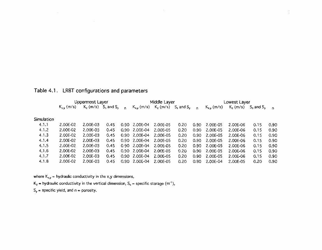
Table 4.1. LRBT configurations and parameters

Uppermost Layer Middle Layer Lowest LayerKx,y (mis.) Kz (mis) 55 and Sy n Kx,y (mis) Kz (mis) S5 and Sy n Kx,y (mis) Kz (mis) S5 and Sy n

Simulation4.1.1 2.00E-02 2.00E-03 0.45 0.90 2.00E-04 2.00E-OS 0.20 0.90 2.00E-05 2.00E-06 0.15 0.904.1.2 2.00E-02 2.00E-03 0.45 0.90 2.00E-04 2.00E-OS 0.20 0.90 2.00E-05 2.00E-06 0.15 0.904.1.3 2.00E-02 2.00E-03 0.45 0.90 2.00E-04 2.00E-OS 0.20 0.90 2.00E-OS 2.00E-06 0.15 0.904.1.4 2.00E-02 2.00E-03 0.45 0.90 2.00E-04 2.00E-05 0.20 0.90 2.00E-OS 2.00E-06 0.15 0.904.1.5 2.00E-02 2.00E-03 0.45 0.90 2.00E-04 2.00E-05 0.20 0.90 2.00E-OS 2.00E-06 0.15 0.904.1.6 2.00E-02 2.00E-03 0.45 0.90 2.00E-04 2.00E-OS 0.20 0.90 2.00E-05 2.00E-06 0.15 0.904.1.7 2.00E-02 2.00E-03 0.45 0.90 2.00E-04 2.00E-OS 0.20 0.90 2.00E-05 2.00E-06 0.15 0.904.1.8 2.00E-02 2.00E-03 0.45 0.90 2.00E-04 2.00E-OS 0.20 0.90 2.00E-04 2.00E-OS 0.20 0.90

where Kx,y = hydraulic conductivity in the x,y dimensions,

Kz = hydraulic conductivity in the vertical dimension, 55 = specifie storage (m' I),

Sy = specifie yield, and n = porosity.

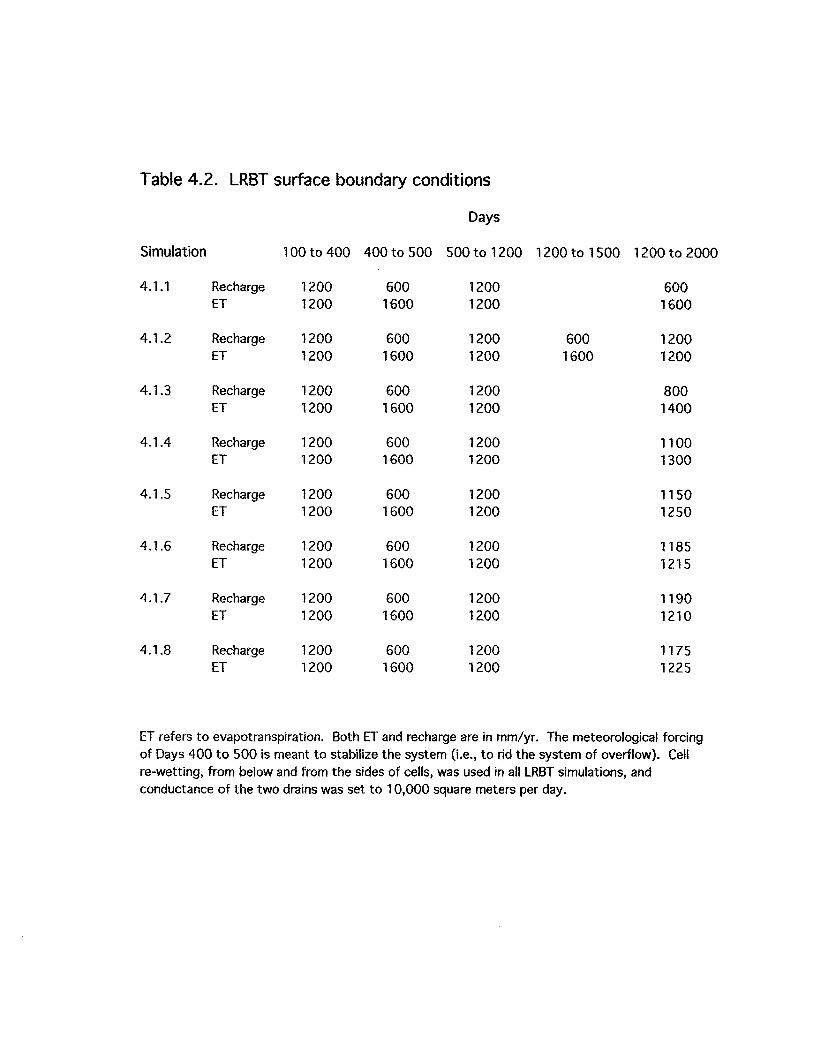
Table 4.2. LRBT surface boundary conditions

Days

Simulation 100 to 400 400to 500 500 to 1200 1200 to 1500 1200 to 2000

4.1.1 Recharge 1200 600 1200 600ET 1200 1600 1200 1600

4.1.2 Recharge 1200 600 1200 600 1200ET 1200 1600 1200 1600 1200

4.1.3 Recharge 1200 600 1200 800ET 1200 1600 1200 1400

4.1.4 Recharge 1200 600 1200 1100ET 1200 1GOO 1200 1300

4.1.5 Recharge 1200 600 1200 11 saET 1200 1600 1200 1250

4.1.6 Recharge 1200 600 1200 1185ET 1200 1600 1200 1215

4.1.7 Recharge 1200 GOa 1200 1190ET 1200 1600 1200 1210

4.1.8 Recharge 1200 GaO 1200 1175ET 1200 1600 1200 1225

ET refers to evapotranspiration. Both ET and recharge are in mm/yr. The meteorological forcingof Days 400 to 500 is meant to stabilize the system (Le., to rid the system of overflow). Cellre-wetting, from below and from the sides of ceUs, was used in ail LRBT simulations, andconductance of the two drains was set to 10,000 square meters per day.

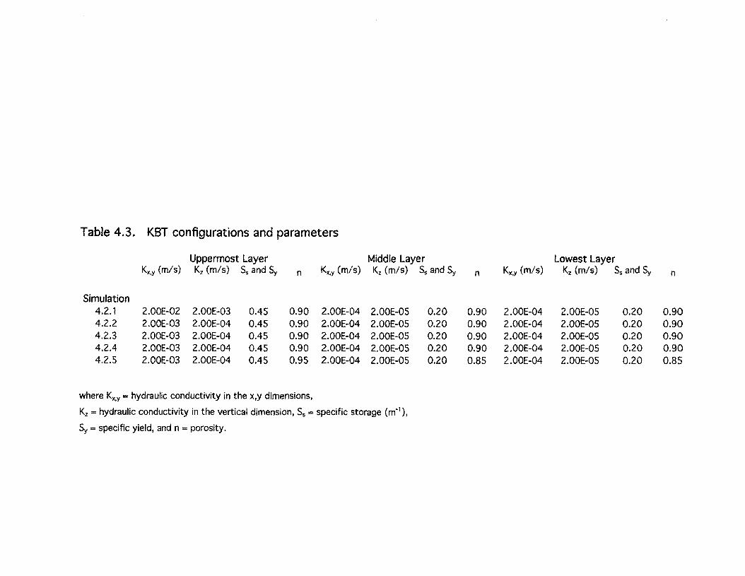
Table 4.3. KBT configurations and parameters

Uppermost Layer Middle Layer Lowest LayerKx.y (mis) Kz (mis) 55 and Sy n Kx,y (mis) Kz (mis) 5s and Sy n Kx•y (mis) Kz (mis) 5s and 5y n

Simulation4.2.1 2.00E-02 2.00E-03 0.45 0.90 2.00E-04 2.00E-OS 0.20 0.90 2.00E-04 2.00E-OS 0.20 0.904.2.2 2.00E-03 2.00E-04 0.45 0.90 2.00E-04 2.00E-OS 0.20 0.90 2.00E-04 2.00E-OS 0.20 0.904.2.3 2.00E-03 2.00E-04 0.45 0.90 2.00E-04 2.00E-OS 0.20 0.90 2.00E-04 2.00E-OS 0.20 0.904.2.4 2.00E-03 2.00E-04 0.45 0.90 2.00E-04 2.00E-OS 0.20 0.90 2.00E-04 2.00E-OS 0.20 0.904.2.5 2.00E-03 2.00E-04 0.45 0.95 2.00E-04 2.00E-OS 0.20 0.85 2.00E-04 2.00E-OS 0.20 0.85

where Kx,y = hydraulic conductivity in the x,y dimensions,

Kz =hydraulic conductivity in the vertical dimension, 55 =specifie storage (m'I),

Sy =specifie yield, and n =porosity.

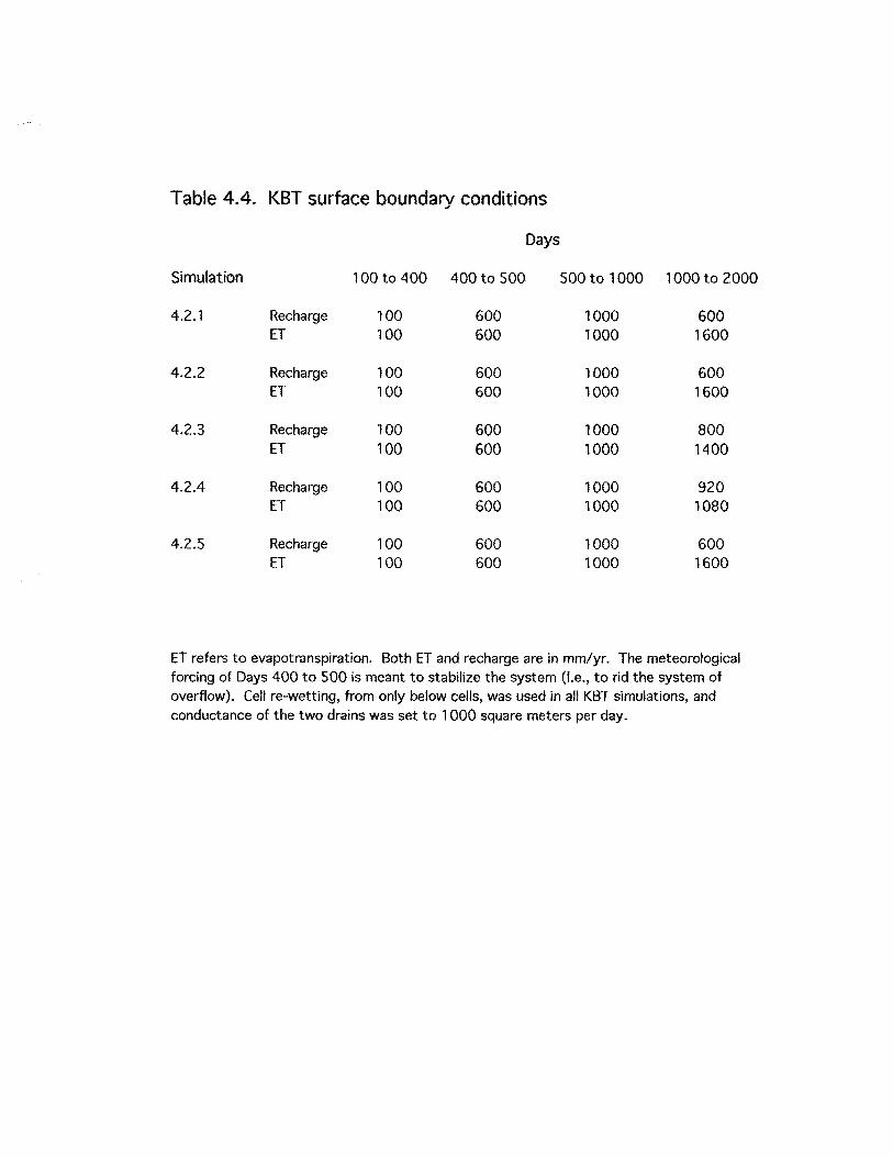
Table 4.4. KBT surface boundary conditions

Days

Simulation 100 to 400 400 to 500 500 to 1000 1000 to 2000

4.2.1 Recharge 100 600 1000 600ET 100 600 1000 1600

4.2.2 Recharge 100 600 1000 600ET 100 600 1000 1600

4.2.3 Recharge 100 600 1000 800ET 100 GOO 1000 1400

4.2.4 Recharge 100 600 1000 920ET 100 600 1000 1080

4.2.5 Recharge 100 600 1000 600ET 100 600 1000 1600

ET refers to evapotranspiration. Both ET and recharge are in mm/yr. The meteorologicalforcing of Days 400 to 500 is meant to stabilize the system (I.e., to rid the system ofoverflow). Cell re-wetting, from only below celfs, was used in ail KBT simulations, andconductance of the two drains was set to 1000 square meters per day.

4.1 LRBT Simulations

4.1.1 Extreme drought conditions

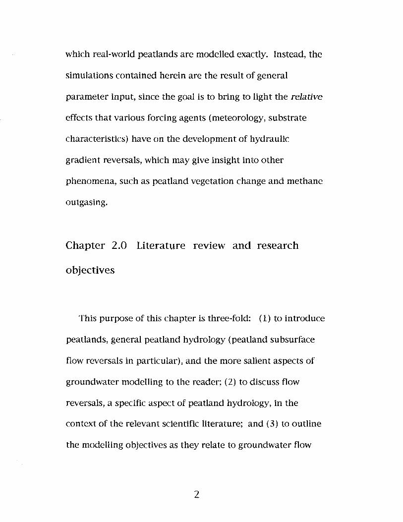
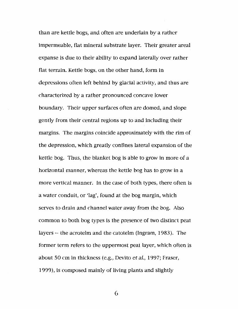
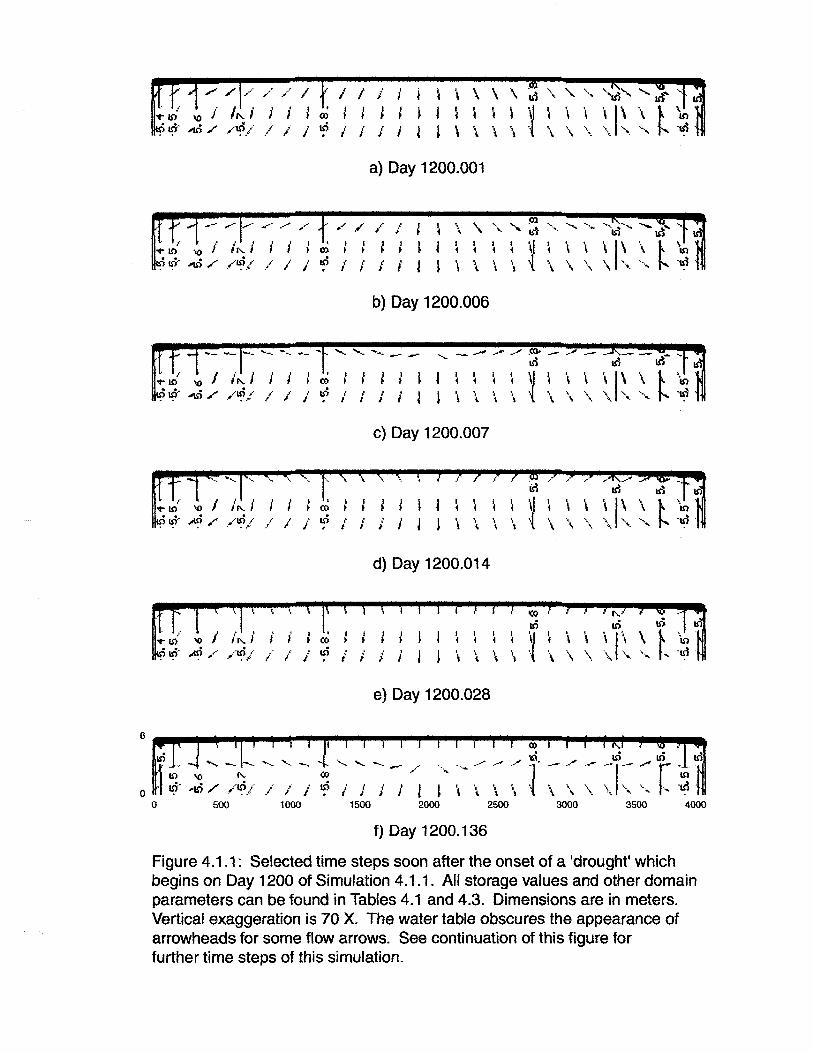
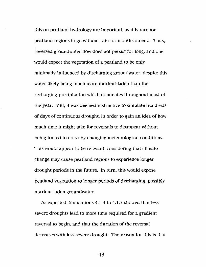
Figure 4.1.1 shows the model domain of a LRBT bog

(Simulation 4.1.1) comprising a 50 cm-thick, relatively high-K

acrotelm layer (Table 4.1), and a 5.3-to-5.5 cm-deep catotelm.

The catotelm had twenty-one layers and two K zones: the

upper catotelm zone being nine layers (2.3 m to 2.5 m) deep

and the lower zone being twelve layers (3.0 m) deep. Within

each K zone, Kx, KY' and ~ values are constant from ceU to ceU,

and ~ is one order of magnitude lower than both Kx and Ky.

After sorne initial adjustment of P and ET early in the

simulation (Table 4.2), the bog achieved a stable state (ôS/ô t

= 0), long before Day 1200. (The adjustment consisted of

lowering P and raising E in order to de-water the system,

whlch had been overflowing from the beginning.

Subsequently, P and E were made to match each other in

magnitude -- a situation which does not occur in peatlands

most of the year, but which does occur during the late spring-

26

1 <" / 1 1 l' J " \ \ \,(0

\ " " ....'Id" " lit .... ,; Id1

,~ \

~1 " \ î\ ' l \co l

~,. "~' .~j ~ i j j j ~ \ \ '\ ... \. \ '\\.a) Day 1200.001

..... ~' '0 / if'..' i i l.. ~~ ,u) /" ..../t?0"/ /.. i' l

.' ,/ / ,.... l l \,

",01

' . ....... .......·~·Id··... - 1Sl'" -.'. -.... Id ",,. l 1 1 1

~1 \ '\

~ I~., \. l \(l) l • • ln~ " j " i l ! \ " ,

... " \ \ '.', '1Sl '. 1 ; \ \ \

b) Day 1200.006

................ --._.-..... U) '0 1 if'.. i , , 1 ~ 1 1 1 J l• \&. .-ID./' /~ / / " J' ~ ( " ( 1 1. . . . .• • 1 1; i

--- ~ - .•- : -- ~....- Id-~ - Id- '.

1 \ \ '\ ~ ~ ~ ~ ~I~ ~ ~ ~

f) Day 1200.136

Figure 4.1.1: Selected time steps soon after the onset of a 'drought' whichbegins on Day 1200 of Simulation 4.1 .1. Ali storage values and other domainparameters can be found in Tables 4.1 and 4.3. Dimensions are in meters.Vertical exaggeration is 70 X. The water table obscures the appearance ofarrowheads for sorne flow arrows. See continuation of this figure forfurther time steps of this simulation.

·1

i~;i/i.~ i i ~.....~)~·~~·l-7.i~~u'"ro:~;--,'---lo....,ro~---:::...J..-.;'-rr-''--'----'~I

g) Day 1200.199

1 t t r"t t u:i

'W-'-'--.,,.----.,r----"!,---,,-----.,r-~-- .~., -- -·k~---'---'-.....,!~ ~~

h) Day 1200.604

i) Day 1200.872

j) Day 1211.263

k) Day 1300.470

---'~r------'ll,r---' "1500 2000 2500

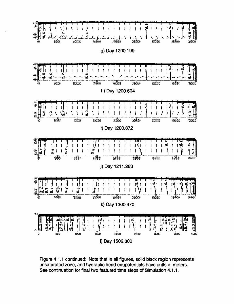
1) Day 1500.000

Figure 4.1.1 continued: Note that in ail figures, solid black region representsunsaturated zone, and hydraulic head equpotentials have units of meters.See continuation for final two featured time steps of Simulation 4.1.1 .

1 ~ 1Irll t 1

"='{,..'----'---"'---,F"""'-..o.=:...t---,~~_'__,;LiJlir-t-J...~--t,r----'-.J,,-..:;;....L:::.:-.J..i~r-~'---~t~"f4X~ t4.Ü):~J:~)

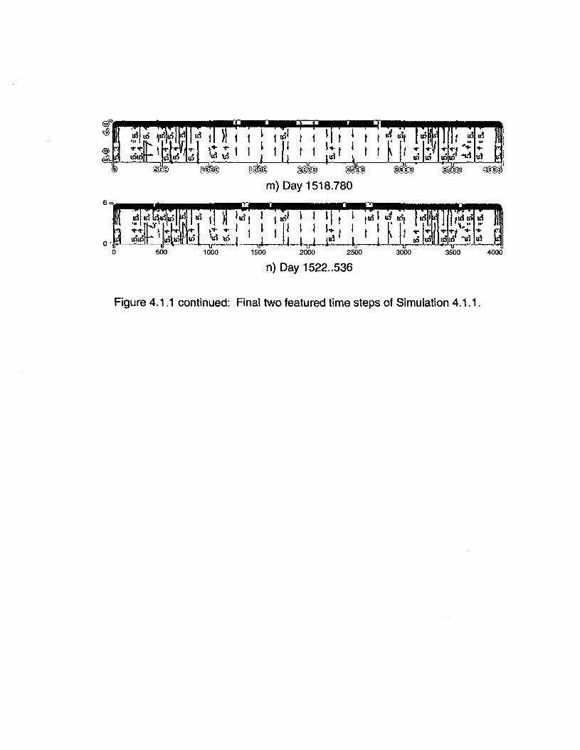
m) Day 1518.780

n) Day 1522..536

Figure 4.1.1 continued: Final two featured time steps of Simulation 4.1.1.

early summer months in eastem North America, when

hydraulic gradient reversaIs are likely to occur.) A

meteorological deficit of 1000 mm/yr was then simulated, via

the lowering of precipitation from the pre-drought value of

1200 mm/yr to a value of 600 mm/yr, and via the raising of

evapotranspiration from the pre-drought value of 1200

mm/yr to a value of 1600 mm/yr.

Figure 4.1.1-a is still early enough in the drought that it

shows the system's pre-drought flow pattern, which generally

is downwards and outwards, from the centre of the bog to its

margins. Note that the difference in hydraulic head between

the uppermost cell in column 57 (horizontal centre of the bog)

and its lowermost cell of the same column is only 0.00023 m

at this point in time. Aiso note that the water table eievation

at the bog's centre is about 5.8 m. Between seven and eight

minutes later (see Figure 4.1.1-c and section 4.1.4 for a

discussion of why such a rapid reversaI occurs in the model,

but not in the field), however, a reversaI of the usual

'downwards and outwards' flow pattern occurs throughout

much of the domain. More specifically, Figure 4.1.1 shows this

27

reversaI ta be limited ta the acratelm and ta the very

uppermost portion of the uppermost catotelm Kzone. AIso,

except for the very center of the bog, the reversaI occurs from

one end of the bog to the other. (Note that the focus

throughout this thesis will be away from the very ends of the

various bogs, in an simulations, since the drains are Iocated

here and they likely interfere with flow patterns in their

Immediate surroundings.) At the very center, flow still is

downwards, as in a) and b) of Figure 4.1.1 , but there is a

noticeable Iaterai component to the flow vectors. By Day

1200.006 (Figure 4.1.1-d), which is about only ten minutes

Iater, flow even at the bog's center (2000 meters from its

edges) is very clearly upwards, and the upward flow shown in

Figure 4.1.1-c is even stronger (Le., more vertical) from one

end of the bog to the other. While hydraulic head at the top

of the bog is decreasing at this point, note that head at the

bottom of the bog has not changed yet, and likely is the reason

for the flow reversaI. However, the reversaI still hasn't made

its way down the peat profile. Figure 4.1.1-e shows even

stronger upward flow, along with no noticeable downward

28

progression of the flow reversaI. On the other hand, Figure

4.1.1-f, which is 199 minutes into the 'drought', indeed shows

such a downward progression, with the reversaI reaching the

very uppermost portion of the lower catotelm zone, though

not yet around the 2000 meter horizontal mark of this zone.

At this point, flow near the bog's surface is almost aH vertical,

while flow deeper down still has sorne horizontal tendency. At

the very bottom of the bog, flow doesn't appear to be any

different than that of Figure 4.1.1-a, which is to say that it is

downwards and outwards. About ninety minutes later (Le.,

about 286 minutes into the 'drought'), Figure 4.1.1-g shows

that flow halfway down the peat profile has 10st its horizontal

tendency, and now is almost compIeteIy vertical. By this

point, hydraulic head in the uppermost ceH of column 57 has

decreased from its "original" value by only 0.00022 m, while

the lawermast ceH in the same column has remained the same.

By Day 1200.604 (Figure 4.1.1-h), which is about 864 minutes

inta the 'drought', upwards flow finally can be observed at the

very bottom of the peat profile. In fact, at the 2000 meter

mark, flow is more upward-tending than is the flow ta its sides

29

(e.g., at the 1000 m and 3000 m marks). Flow all along the

lower boundary of the domain continues to be significantly

horizontal. Figure 4.1.1-1 ,shows that flow on Day 1200.872 is

almost completely vertical throughout the bog, including its

lowermost reaches, where flow now is only slightly horizontal,

and where hydraulic head finally has begun to decrease. Ten

days later (Figure 4.1.1-j), aU flowappears to be upward,

which remains true up until 300 days into the 'drought' (see

Figures 4.1.1-k and -1). Note that, during these 300 days, head

throughout the system continues to drop, and the water table

therefore predictably flattens. By Day 1518.780 (Figure 4.1.1­

m), the head value in the uppermost cell of column 57 nears,

though is stilliess than, that of its 10wermost cell -- the

difference is 0.00529 m. This changes by the next time step

(Day 1522.536, Figure 4.Ll-a), when flow at and about the

horizontal center (2000 meter mark) of the bog finally

becomes downward again; the head difference between the

uppermost cell and lowermost cell in column 57 now is only

0.00282 m, which is in the range of differences observed on

Day 1200, just after the onset of 'drought'. Note that the

30

water table now is completely fiat, and that the highest

hydraulic head difference (between the uppermost and

lowermost ceUs in column 57) occurred roughly after Day

1210 but before Day 1300; during this time, this difference

was in the range of only 0.7 cm.

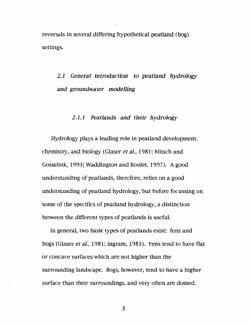
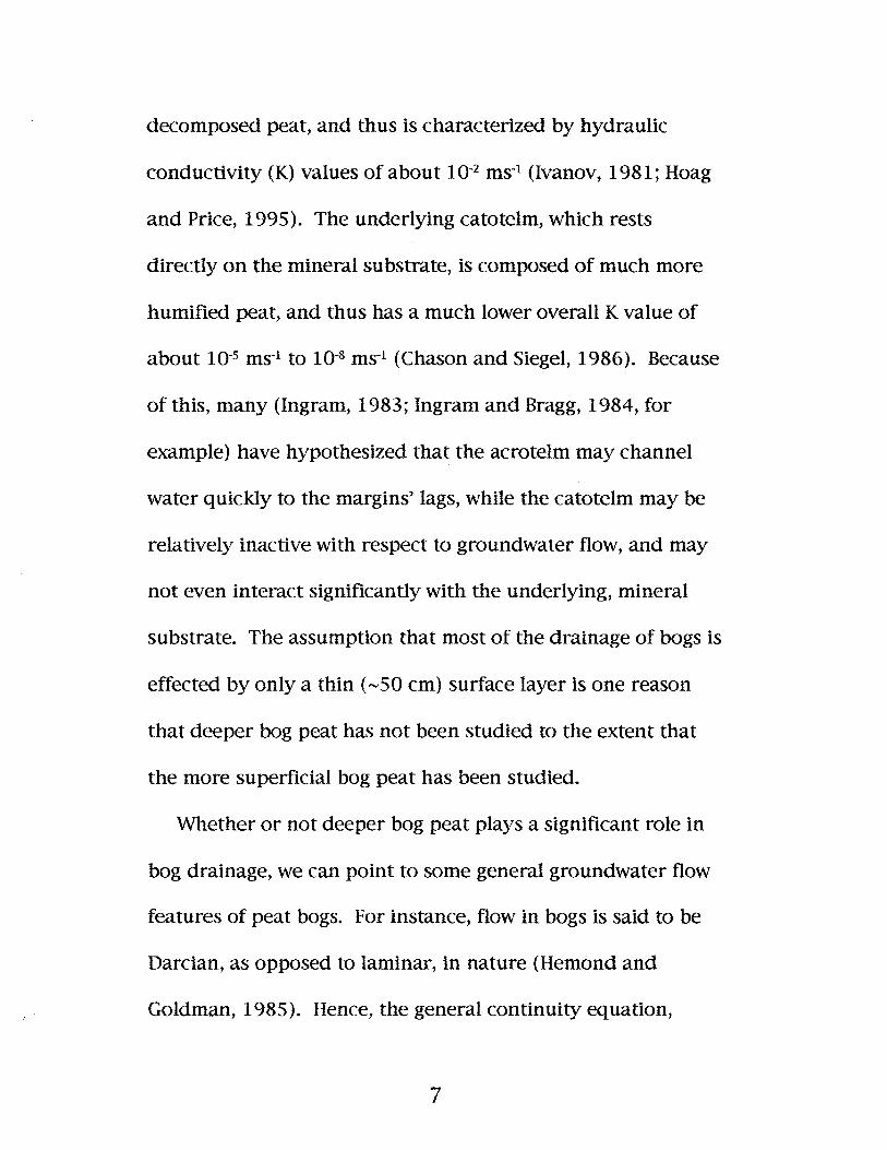
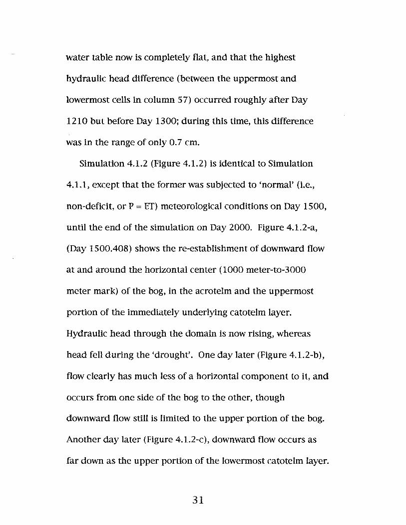
Simulation 4.1.2 (Figure 4.1.2) is identical to Simulation

4.1.1, except that the former was subjected to (normal' (Le.,

non-defictt, or P = ET) meteorological conditions on Day 1500,

untU the end of the simulation on Day 2000. Figure 4.1.2-a,

(Day 1500.408) shows the re-establishment of downward flow

at and around the horizontal center (1000 meter-to-3000

meter mark) of the bog, in the acrotelm and the uppermost

portion of the immediately underlying catotelm layer.

Hydraulic head through the domain is now rising, whereas

head feU during the (drought'. One day later (Figure 4.1.2-b),

fiow clearly has much less of a horizontal component to it, and

occurs from one side of the bog to the other, though

downward f10w still is limited to the upper portion of the bog.

Another day later (Figure 4.1.2-c), downward flow occurs as

far down as the upper portion of the lowermost catotelm layer.

31

a) Day 1500.408

b) Day 1501.462

c) Day 1502.527

d) Day 1503.640

e) Day 1504.368

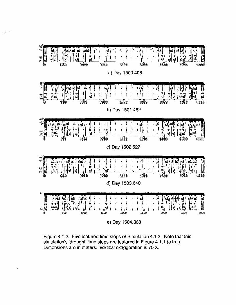
Figure 4.1.2: Five featured time steps of Simulation 4.1.2. Note that thissimulation's 'drought' time steps are featured in Figure 4.1.1 (a to 1).Dimensions are in meters. Vertical exaggeration is 70 X.

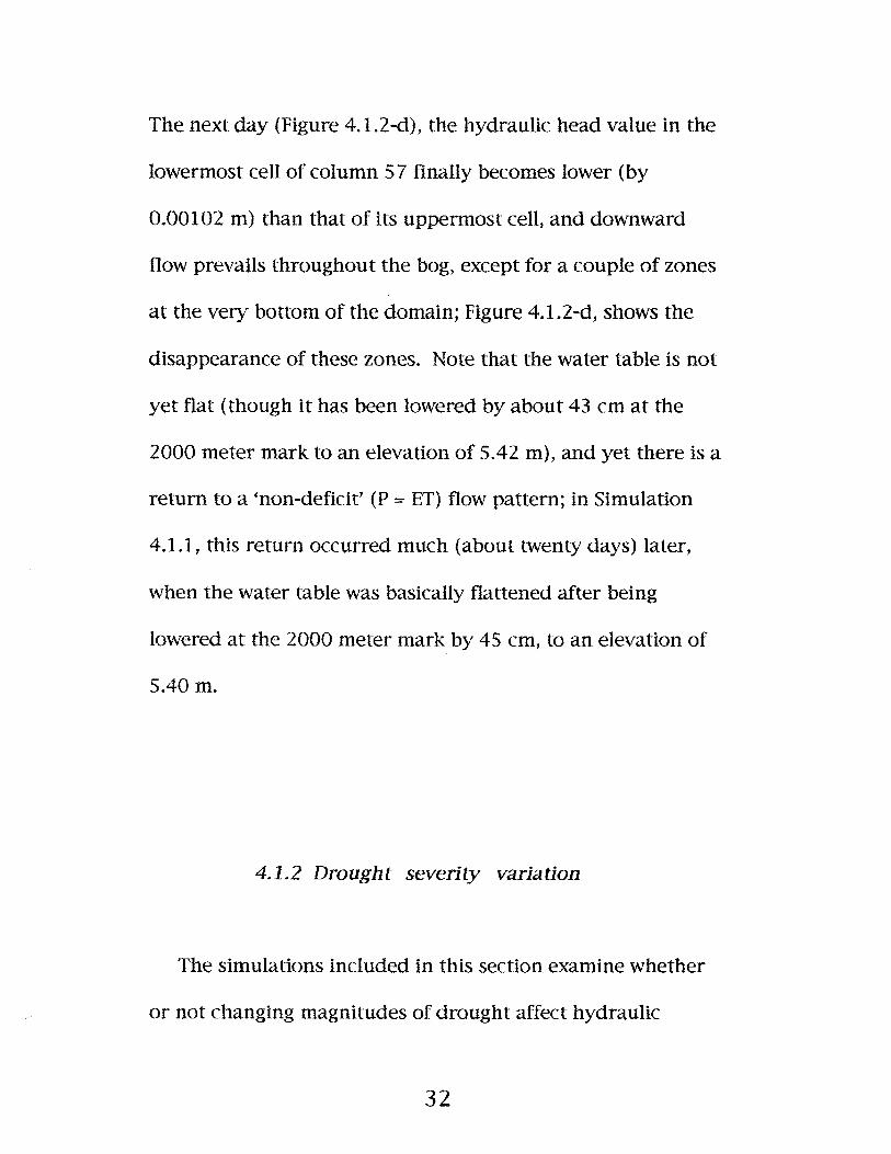
The next day (Figure 4.1.2-d), the hydraulic head value in the

lowermost ceIl of column 57 finally becomes lower (by

0.00102 m) than that of its uppermost ceH, and downward

flow prevails throughout the bog, except for a couple of zones

at the very bottom of the domain; Figure 4.1.2-d, shows the

disappearance of these zones. Note that the water table is not

yet flat (though it has been lowered by about 43 cm at the

2000 meter mark to an elevation of 5.42 m), and yet there is a

return to a 'non-deficit' (P = ET) flow pattern; in Simulation

4.1.1, this return occurred much (about twenty days) later,

when the water table was basically flattened after being

lowered at the 2000 meter mark by 45 cm, to an elevation of

5.40 m.

4.1.2 Drought severity variation

The simulations included in this section examine whether

or not changing magnitudes of drought affect hydraulic

32

gradient reversaIs differently. Table 4.2 shows how the

magnitude of drought is decreased from one simulation to the

next. Another aim is to determine whether or not there exists

a definite minimum drought magnitude requirement for the

onset of a hydraulic gradient reversaI, or rather a range of

magnitudes providing various reversaI 'strengths.'

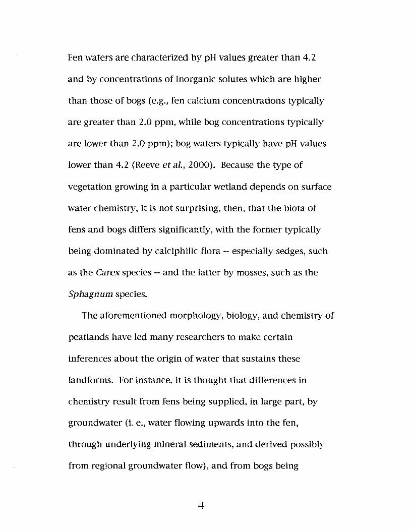
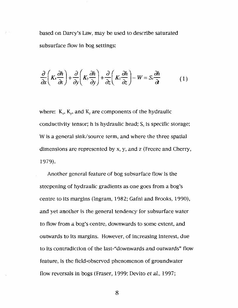
Figure 4.1.3, shows the flow patterns resulting from a

simulation which matches Simulation 4.1.1 , in every way

except for the drought magnitude, which now has been set to

600 mm/yr (800 mm/yr of precipitation, 1400 mm/yr of

evapotranspiration) instead of 1000 mm/yr. (This 600 mm/yr

deficit approximates the fifty-day 1998 meteorological balance

of 504 mm/yr observed at Fraser's (1999) Mer Bleue field site.

(Of the fifty days, only the Iast forty were characteristic of

drought conditions, thus making 504 mm/yr an underestimate

during this true drought period.) ET being larger than P

(during drought) in aIl of the simulations is consistent with

observed ET and P during summer months in peatland areas.

Pre-drought modelIed equivalence of ET and P, though not

observed in the field during non-summer months, can occur

33

l1 1

1/ ;;, /

~/ "'.... .1/ '" l.l' 1 ;'

t

a) Day 1200.006

b) Day 1200.014

..., " , ''"'~. ",... ./

t;:;, IT~'l

1 l" i i i l ~ j ~i

~ \ '1'0 co !

,~~Ld' .ou) /' /ID/ l " / ID 1 r 1 1Il ~ '1 " JL " '. \ \ ", l',. ' ...__ n:- ~1 • 1 • i 1 \ "

. li . _il . . Je _IJJJ 'é1l!;sJ tM.ww 1!'é1S§ '~1 ~~1 e:.2.®.!!J ~.2.\

c) Day 1200.017

d) Day 1200.418

e) Day 1200.726

\ \. \

(l) ,

ljJt'!"' 1 t~4l""t :J4LO t .Il' Il'~/' ID

.t ,1 l.f .••..• //. /.l''''_~

=?f-'----.,,-~--.,Hr-~---,Hr-----,u'-----,( -, ~

1000 1500 2000 2500 3000 3500 4000

f) Day 1200.872

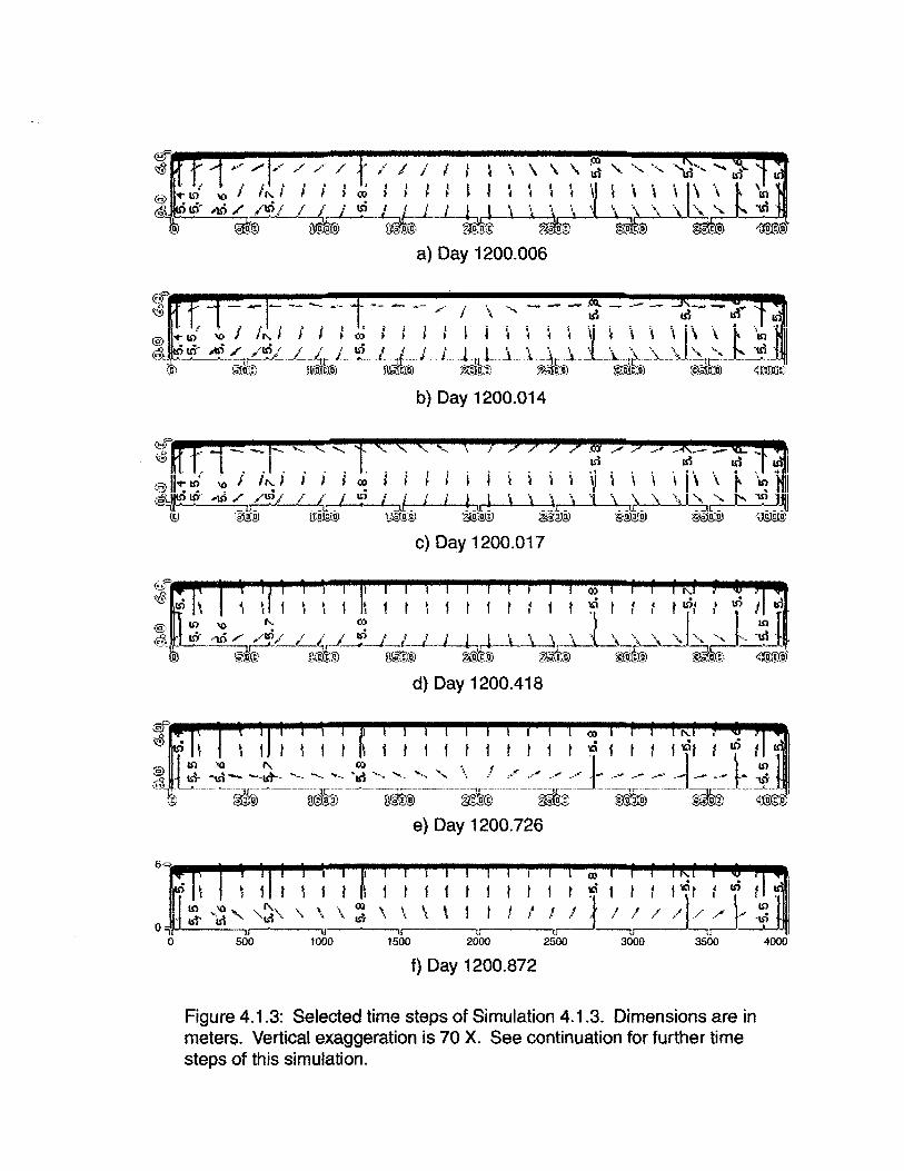
Figure 4.1.3: Selected time steps of Simulation 4.1.3. Dimensions are inmeters. Vertical exaggeration is 70 X. See continuation for further timesteps of this simulation.

g) Day 1248.447

h) Day 1300.466

11 t 1 t 1 t t t t 1 ~ t 1 ~ t tiit t 1 IÔt .

r-_~\_}:,,~~.~~,~t__\_~_g~""~.~.F"t;_)_,~~1.-~~~!~~]-~_t_~~l __-1/-1 t 1~~J~~i) Day 1500.000

DDay 1916.667

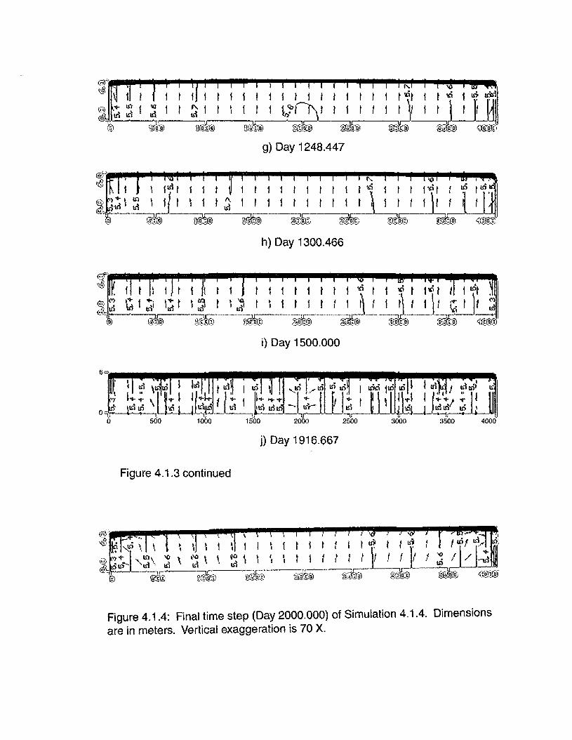
Figure 4.1 .3 continued

lt

•tt 1t 1

•1l

Figure 4.1.4: Final time step (Day 2000.000) of Simulation 4.1.4. Dimensionsare in meters. Vertical exaggeration is 70 X.

for a short period of time leading up ta a drought.) Like

Simulation 4.1.1 , a flow reversaI occurs on the tirst day of

deficit (see Figure 4.1.3-b), and again is limited ta the acrotelm

and to the sides of the horizontal center Hne (2000 m mark) of

the bog. Within about 24 minutes of the onset of 'drought',

the reversaI occurs even at the bog's center Une (see Figure

4.1.3-c). This same pattern occurred less than ten minutes

Îllto the 'drought' of Simulation 4.1.1. Figure 4.1.3-d shows

the flow reversaI making its way down the peat profile, to the

upper portion of the lowermost catotelm layer. The next

figure shows that the reversaI has reached the bottom of that

layer (Le., the bottom of the bog), though flow there still has a

significant horizontal direction. The upward flow in Figure

4.1.3-f has much more of a vettical direction, and this is even

more so in the next three figures. The last figure of Simulation

4.1.3 (Day 1916.667) finally shows a return to downward flow

at the 2000 meter mark of the bog, though this occurs later

than it did in Simulation 4.1.1 (and thus later than it did in

Simulation 4.1.2). Note that the water table isn't quite flat

yet, and that the maximum upper-Iower bog head difference in

34

this simulation was 0.5 cm, around Day 1250. This difference

is 0.3 cm less than that simulated in Simulation 4.1.1, when

the meteorological deficit was 400 mm/yr larger.

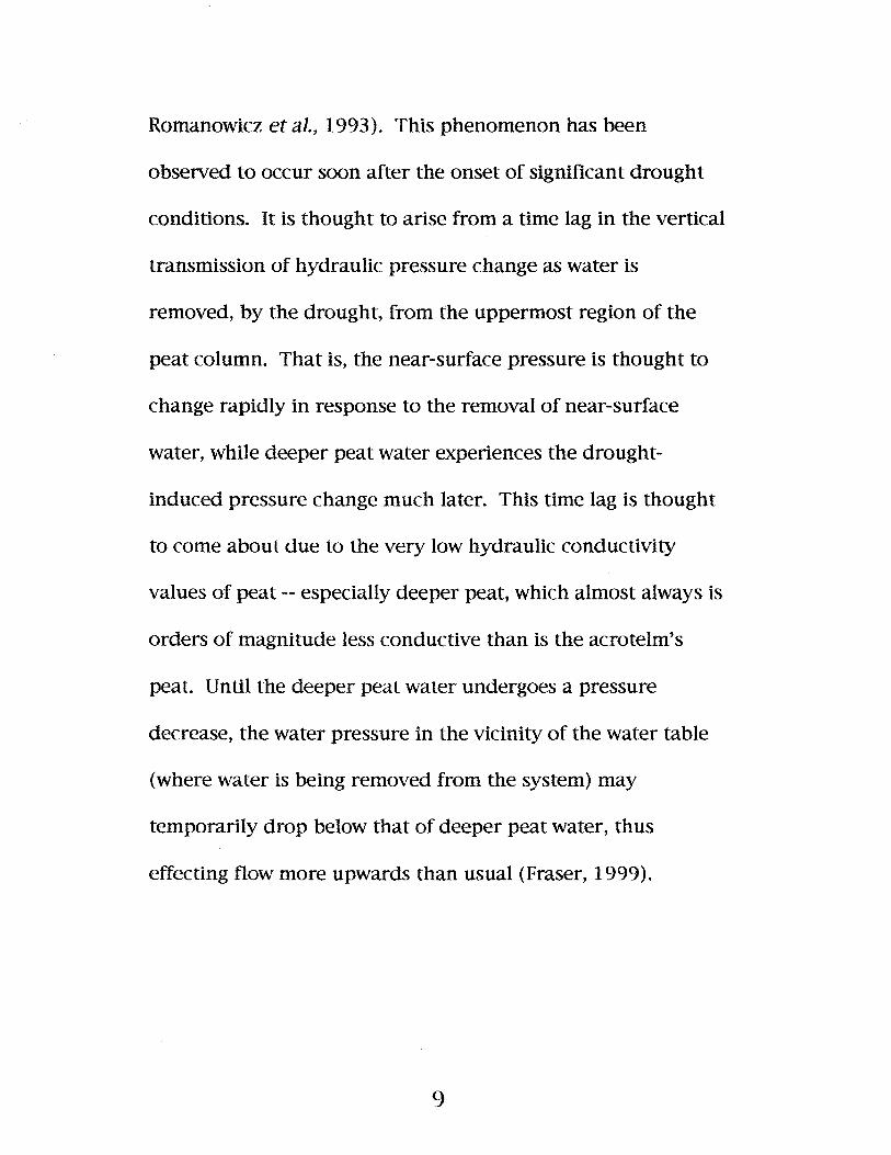
Figure 4.1.4 shows the flow patterns resulting from a

simulation which matches Simulation 4.1.1 in every way

except for the drought magnitude, which now has been set to

200 mm/yr (1100 mmlyr of precipitation, 1300 mm/yr of

evapotranspiration) instead of 1000 mm/yr. This 200 mm/yr

balance is now lower than the 504 mm/yr balance observed by

Fraser (1999). Like Simulation 4.1.1 and Simulation 4.1.2, a

flow reversaI occurs early on in the present simulation, but

this reversaI begins later (58 minutes into Day 1200) and

continues to the end of the simulation (Day 2000). Note that

the water table has not been lowered to the extent that it was

lowered in Simulations 4.1.1 and 4.1.3; in Simulation 4.1.4, on

Day 2000, the water table is observed to have dropped by only

about 15 cm, down to roughly 5.7 m elevation. Thus, the

water table at this time still is clearly mounded. Note also that

the hydraulic head difference, between the uppermost and

lowermost cells in column 57, at this time is only 0.05 cm,

35

indicating that a retum ta downward flow (Le., a hydraulic

gradient reversaI) isn't far off.

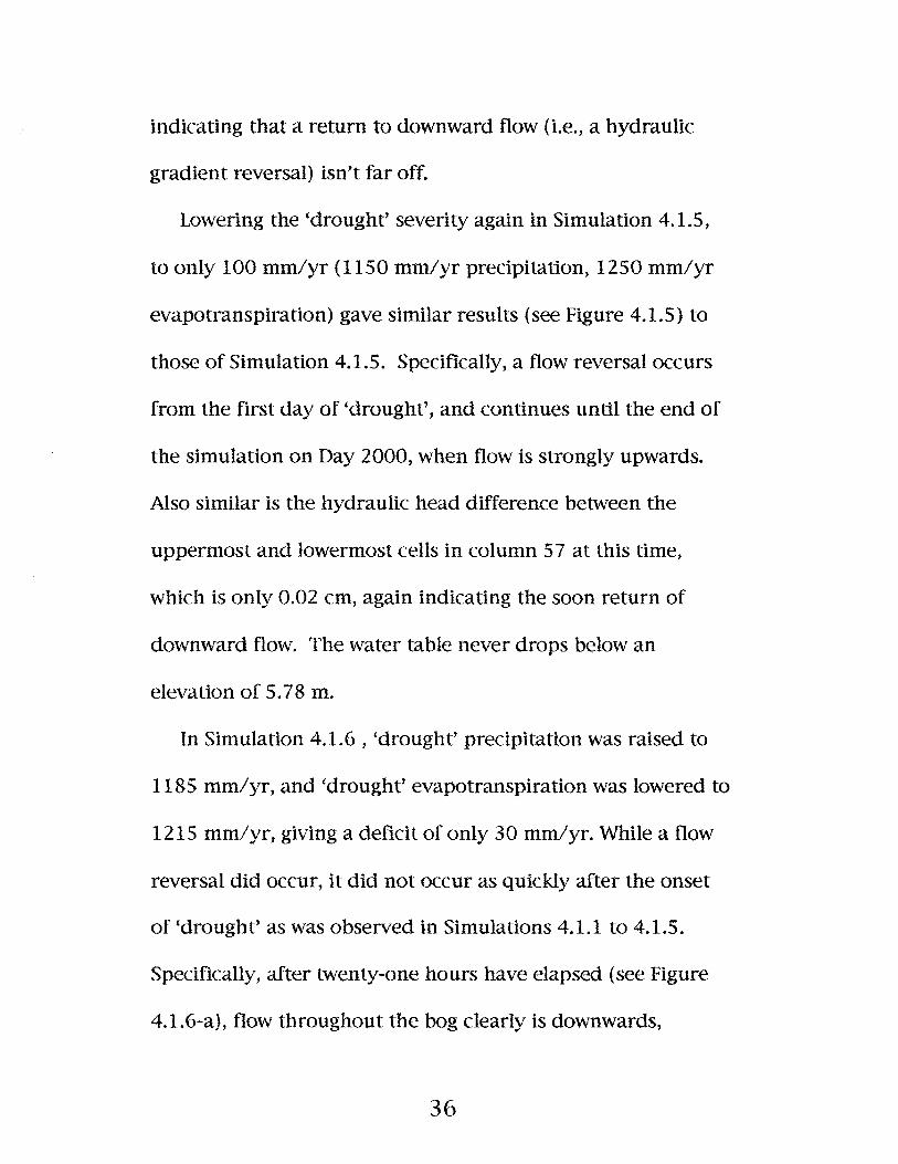
Lowering the 'drought' severity again in Simulation 4.1.5,

to only 100 mm/yr (1150 mm/yr precipitation, 1250 mm/yr

evapotranspiration) gave similar results (see Figure 4.1.5) ta

thase of Simulation 4.1.5. Specifically, a flow reversaI occurs

from the first day of 'drought', and continues until the end of

the simulation on Day 2000, when flow is strongly upwards.

Also similar is the hydraulic head difference between the

uppermost and lowermost ceUs in column 57 at this time,

which is only 0.02 cm, again indicating the soon return of

downward flow. The water table never drops below an

elevation of 5.78 m.

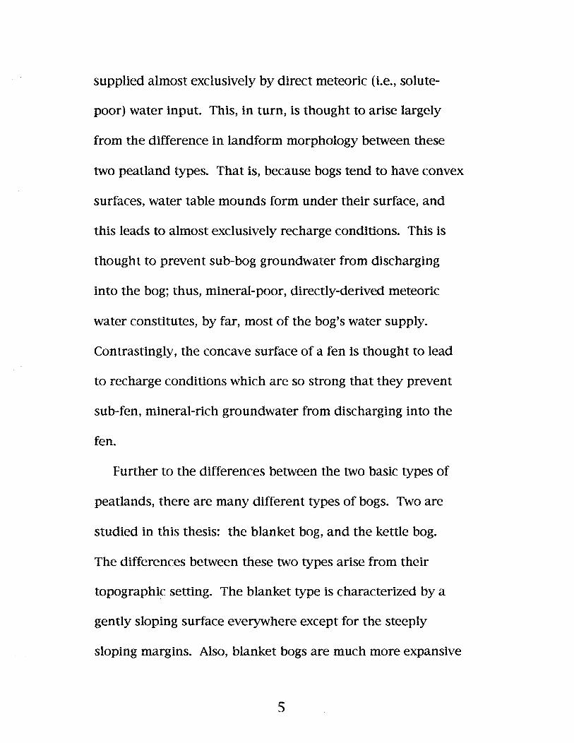
In Simulation 4.1.6 , 'drought' precipitation was raised to

1185 mm/yr, and 'drought' evapotranspiration was lowered to

1215 mm/yr, giving a deficit of only 30 mm/yr. While a flow

reversaI did occur, it did not occur as quickly after the onset

of 'droughf as was observed in Simulations 4.1.1 to 4.1.5.

Specifically, after twenty-one hours have elapsed (see Figure

4.1.6-a), flow throughout the bog clearly is downwards,

36

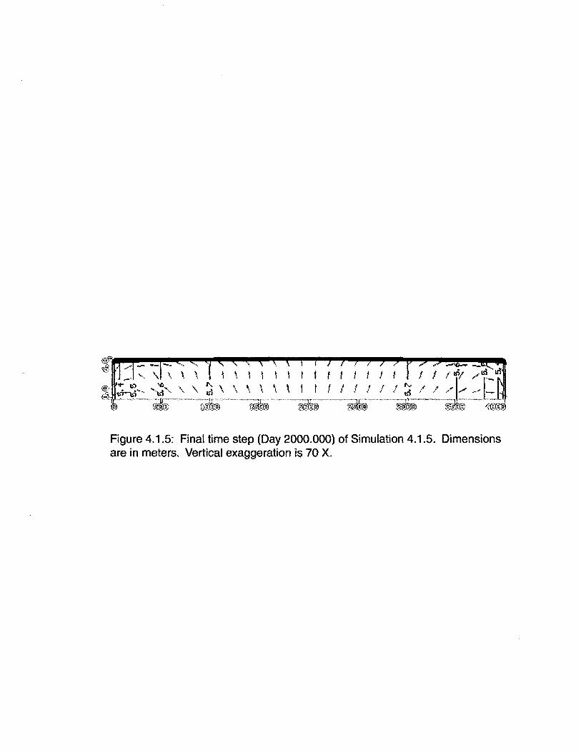
Figure 4.1.5: Final time step (Day 2000.000) of Simulation 4.1.5. Dimensionsare in meters. Vertical exaggeration is 70 X.

a) Day 1200.872

b) Day 1202.615

-- ...- -- ...- J"'".- ....... -- ---"'lo -- --

.-,- - -- .....~ _l~

c) Day 1204.523

d) Day 1205.429

e) Day 1206.516

. -. " \.... " ... t.

-... __ .....- __ .~W" .-.. _ _ ._.- _ ......

1 / ,/ / /LIS'l../ ,.." ./ .,J>ll:.... ,," lSi... ."\fI'l) ca \. /.,. 'O.

o q-i/-J-lt)..;...._-_ld -_-..,;flr-_-ln~....._-_-_-_-..,~,_-_-~1rl~"'_-·_~.,t~'_--~----"'_···---'u,-·--···_·-----,·~ _.... ~- -- -- --,...; -- .. -"d :u

o 500 1000 1500 2000 2500 3000 3500 4000

f) Day 1207.820

Figure 4.1.6: Selected time steps soon after the onset of 'drought' inSimulation 4.1 .6. Dimensions are in meters. Vertical exaggeration is 70 X.See continuation of this figure for further time steps.

g) Day 1216.221

- - - .-\ ... \'" \ \ 1 • .1 ,1 /'1 1 1

'. '-, \ (/ ./..... .••. \ .. •••4l'

~'D:@J1j) .'" ... .:.P'- ._~

h) Day 1258.138

i) Day 1344.673

-_-~____ ".., { '} ,-~_-..f».-~-_~_-

1 ~..... -" -' --- ....... -. .....- ...~ ...... "" "" " l ..--- ~J /" "---~I~"'" .- .'''' -~ -- -- ...... 'an

. t:5· _.~~ - ~ -- -- -- -~- -. -. "'-. \.'. ---- .."'.- .,~ .- - -~ -~ -- ~ ~ ~:t- 1do -t, - -. -' - ..·--1.,---·----11--- -----.---,:- -- ----------u--- ----- -1.~-------'T--- - -.----.r---~-'-

o 500 1000 1500 2000 2500 3000 3500 4000

j) Day 2000.000

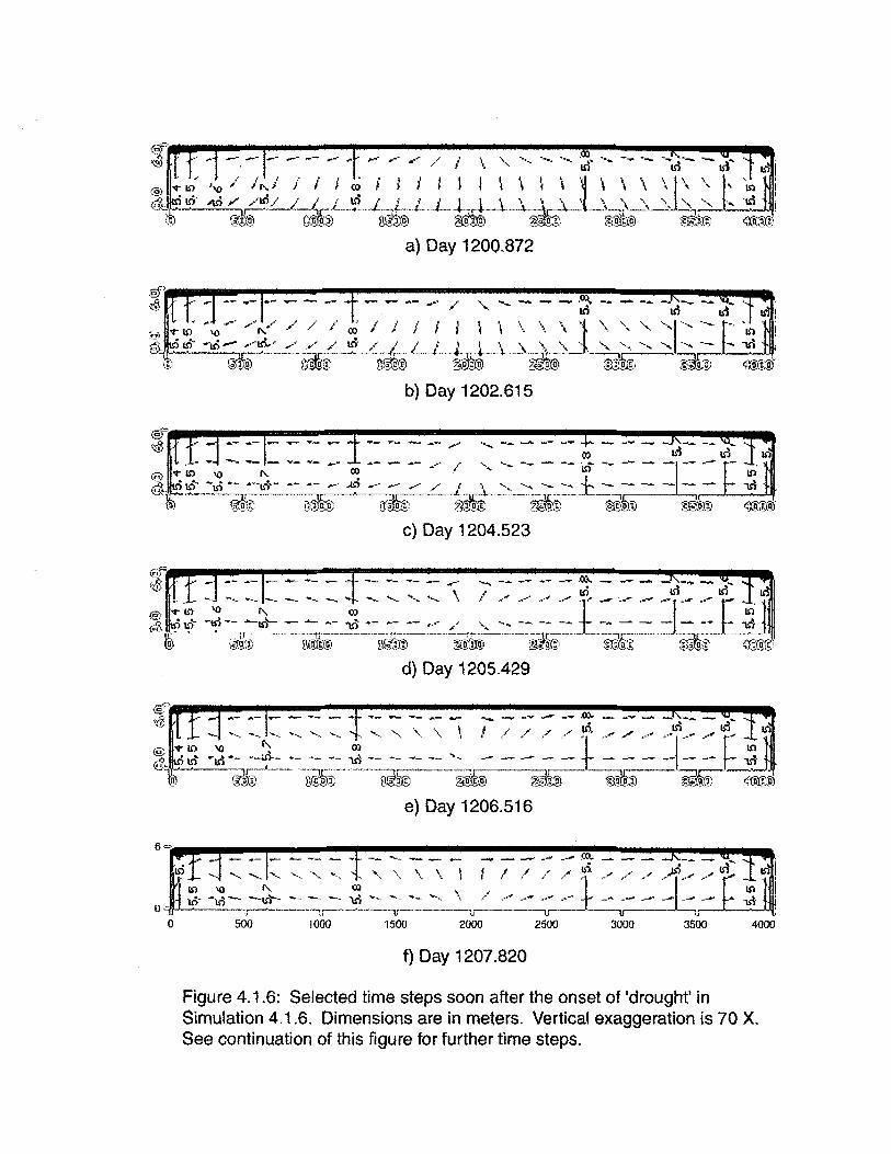
Figure 4.1.6 continued

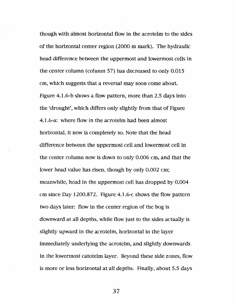
though with almost horizontal flow in the acrotelm to the sides

of the horizontal center region (2000 m mark). The hydraulic

head difference between the uppermost and low€rmost ceUs in

the center column (column 57) has decreased to only 0.015

cm, which suggests that a reversaI may soon come about.

Figure 4.1.6-b shows a flow pattern, more than 2.5 days into

the 'drought', which differs only slightly from that of Figure

4.1.6-a: where flow in the acrotelm had been almost

horizontal, it now is completely so. Note that the head

difference between the uppermost cell and lowermost cell in

the center column now is down to only 0.006 cm, and that the

lower head value has risen, though by only 0.002 cm;

meanwhile, head in the uppermost ceH has dropped by 0.004

cm since Day 1200.872. Figure 4.1.6-c shows the flow pattern

two days later: flow in the center region of the bog is

downward at aIl depths, while flow just to the sides actuaIly is

slightly upward in the acrotelm, horizontal in the layer

immediately underlying the acrotelm, and slightly downwards

in the lowermost catotelm layer. Beyond these side zones, flow

is more or less horizontal at aIl depths. FinaIly, about S.S days

37

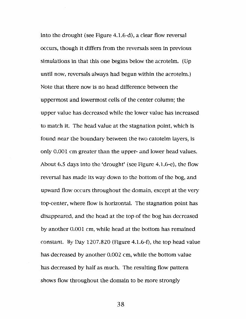
into the drought (see Figure 4.1.6-<1), a clear flow reversaI

occurs, though it differs from the reversaIs seen in previous

simulations in that this one begins below the acrotelm. (Up

until now, reversaIs always had begun within the acrotelm.)

Note that there now is no head difference between the

uppermost and lowermost ceUs of the center column; the

upper value has decreased while the lower value has increased

to match it. The head value at the stagnation point, which is

found near the boundary between the two catotelm layers, is

only 0.001 cm greater than the upper- and lower head values.

About 6.5 days into the 'drought' (see Figure 4.1.6-e), the flow

reversaI has made its way down to the bottom of the bog, and

upward flow occurs throughout the domain, except at the very

top-center, where flow is horizontal. The stagnation point has

disappeared, and the head at the top of the bog has decreased

by another 0.001 cm, while head at the bottam has remained

constant. By Day 1207.820 (Figure 4.1.6-f), the top head value

has decreased by another 0.002 cm, while the bottom value

has decreased by haIf as much. The resulting flow pattern

shows flow throughout the domain to be more strongly

38

upward than in part e). This flow pattern is not unlike that

obsenred by Fraser (1999), though the present, simulated

'drought' is more than an order of magnitude less severe than

that which occurred at his field site in 1998. Sîxteen days into

the 'drought' (see Figure 4.1.6-g), upward flow is even more

pronounced, and the head difference between the top and

bottom of the bog now has doubled to 0.004 cm; while both

head values have continued to decrease since Day 1207, the

upper value decreased by 0.009 cm as the lower value

decreased by 0.007 cm. The flow reversal's strength begins to

wane by Day 1258 (see Figure 4.1.6-h), as evidenced by the

more lateral flow at the top-center of the bog, and by the fact

that the deep head value changed slightly faster (dropped by

0.045 cm) than did the shallow head value, which decreased

by 0.044 cm The shallow-deep head difference reflects this,

as it now has decreased by 0.001 cm, down to only 0.003 cm.

This head difference, along with the head gradient, remains

the same by Day 1344 (see Figure 4.1.6-i), though a re­

establishment of downward flow now can be seen at the

shallow center of the bog, and a re-establishment of lateral

39

flow now occurs just to the sides of center. Although there

still is upward flow throughout much of the deeper peat

profile, it is weakened as the shallow~deephead difference

reverses to 0.001 cm by Day 2000, and downward flow pattern

prevails throughout the shallow portion of the bog. Note that,

since the beginning of this simulation's 'drought', the water

table has lowered by only 0.5 cm.

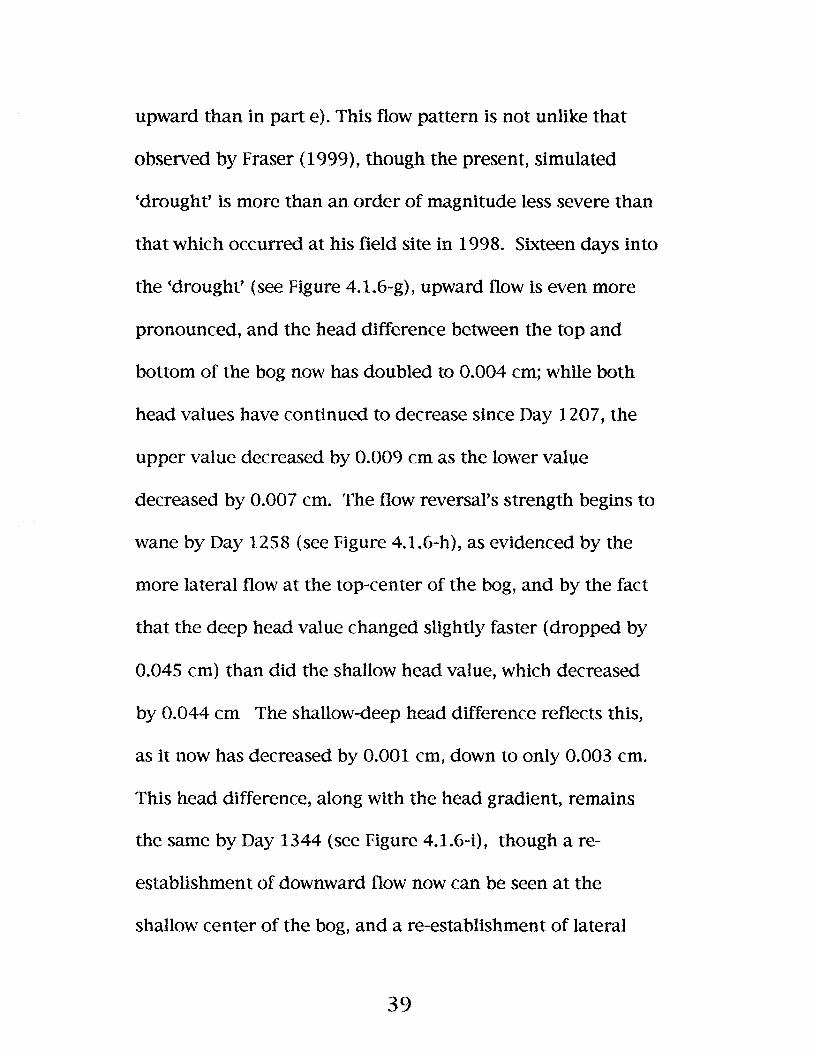
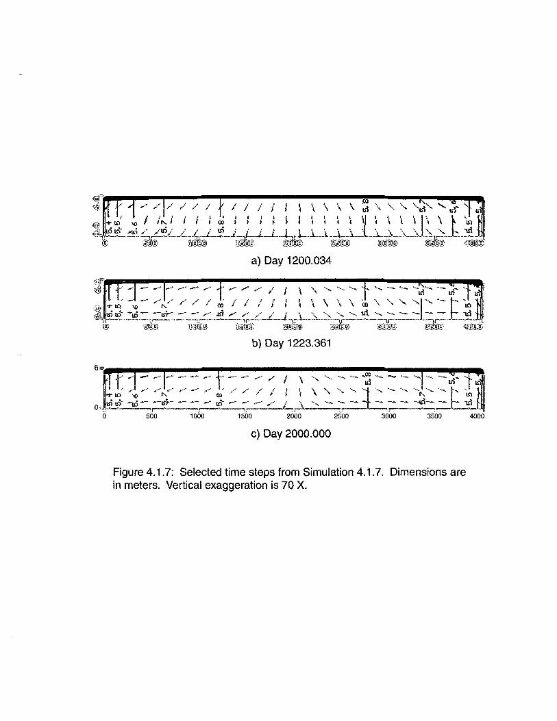
Simulation 4.1.7 (see Figure 4.1.7), which features a

'drought' deficit of only 20 mm/yr, yields no flow reversaI at

aIl. This is the first time, since we began Iowering the deficit

successively from one simulation to the next, that a flow

reversaI has not occurred. From Day 1200.034 ta Day 1223,

the flow pattern throughout the bog acquires a more lateraI

tendency, and the same is true on Day 2000. The end result

(see Figure 4.1.7~c) is a pattern in which flow still is

predominantly downwards. It is important to note, however,

that, despite the meteorological deficit, the water table

actually rose slightly (by 0.5 cm) since the beginning of this

simulation's 'drought'.

40

a) Day 1200.034

" . ,.... ;" ,.J / , " \, "'... ~'" '.., " "... '- "- ~'ld~'" '- Irl- '0 m l'

._....::.:.-----,~ ,,.....-ID~:-. -;-;g-'i=%I~"'-~):"""'::_: ...:.,~_.:~~""'~~-~:D""'~ _~'~~_'~_~O:H;_::~)_~~_O' -~~:_;-,\;]';"'-t-~:_' _:-'~~~ t~b) Day 1223.361

6""~: t"/.. -"01~... ~.~: I-.o~ ~OO~ -_~ ~·.00 t -..~ ~~ ~.:. ;/.. 1 \ '-', '0'00 ~-- '- '~ '- -... '- 0---'.--. -- ~- n~w . ~." - l'.' ~ .' (0 .~ ,,' ". i \ '\. ..... ...... 'Lo ....... "- '.., '00.' .oo~ "'''' ~. 1

", . -- --ur- -- -- __ " , , 0 • • • "', ••-- ,; -- _ -~ -- -- -~.-- _-- ~_ .0

Oc;".~" lfJ .....1$) ~ !J" lj -- lf' -,,-- : .-- --,... ;' _...~\- 'J J '

o 500 1000 1500 2000 2500 3000 3500 4000

c) Day 2000.000

Figure 4.1.7: Selected time steps fram Simulation 4.1.7. Dimensions arein meters. Vertical exaggeration is 70 X.

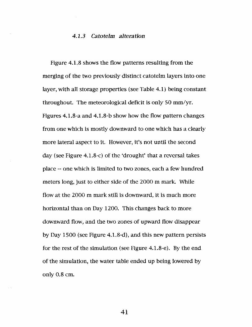
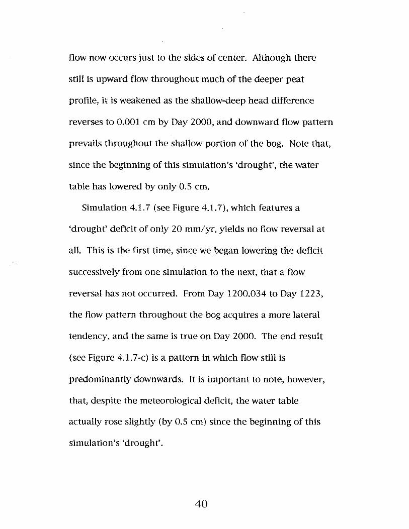
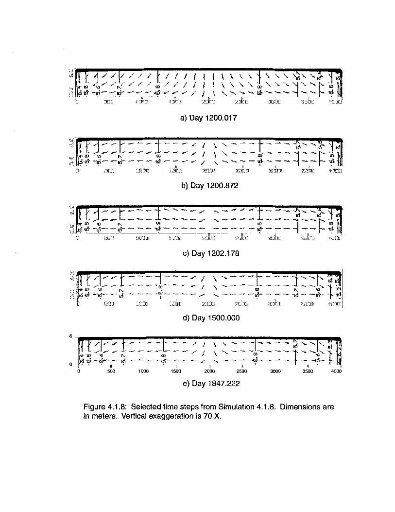
4.1.3 Catotelm alteration

Figure 4.1.8 shows the flow patterns resulting from the

merging of the two previously distinct catotelm layers into one

layer, with aIl storage properties (see Table 4.1) being constant

throughout. The meteorological deficit is only 50 mm/yr.

Figures 4.1.8-a and 4.1.8-b show how the flow pattern changes

from one which is mostly downward to one which has a clearly

more lateral aspect to it. However, it's not until the second

day (see Figure 4.1.8-c) of the 'drought' that a reversaI takes

place -- one which is limited to two zones, each a few hundred

meters long, just to either side of the 2000 m mark. While

flow at the 2000 m mark still is downward, it is much more

horizontal than on Day 1200. This changes back to more

downward flow, and the two zones of upward flow disappear

by Day 1500 (see Figure 4.1.8-d), and this new pattern persists

for the rest of the simulation (see Figure 4.1.8-e). By the end

of the simulation, the water table ended up being lowered by

only 0.8 cm.

41

III ,c- 1It"~; i'lO"'- /" ",/ / /" ./ ~ ./ / / 1:J "ur -uï- -.rr-- .-.- -- ~........- J.-' /~ 11 U

b :lUCI il :JU:1 i\ "iO

t1 ~

111

\

:~:.Jt:.Ii

a) Day 1200.017

1 \1 \/ .....3ITJll'l

b) Day 1200.872

------ .......L" lit" ID '0 '" 00

"-ut --aô- -!n-- - ~- - .".1- ~ ~- - - -'-

c) Day 1202.178

... ~-- ~ ---- - -- ....- .....- .......co~ -- .-- .,-r

.~ ID '0 '" "~ "-ut -I{)-"-'.- uf - - - ~- - -

D UQ] ::t:::Π::uhrr

d) Day 1500.000

e) Day 1847.222

Figure 4.1.8: Selected time steps tram Simulation 4.1.8. Dimensions arein meters. Vertical exaggeration is 70 X.

When the deficit was lowered to 0111y 20 mm/yr

(Simulation 4.1.9), no reversaI occurred, but note that the

water table indeed did faH with time, which wasn't the case in

Simulation 4.1.7.

When the deficit was raised from 50 mm/yr to 600 mm/yr,

the result was a progression of flow patterns almost identicaI

to that of Simulation 4.1.3, which also has a deficit of 600

mm/yr.

4.1.4 Discussion of LRBT simulations

The first two simulations, 4.1.1 and 4.1.2, when considered

together, clearly show that a precipitation event can bring

back, as occurred in Fraser (1999), (downwards and outwards'

flow more quickly than if a system is aHowed to continue

without such drought relief. The reason for this return is the

hydraulic head contribution, made by precipitation, to the

upper portions of the peat column. Head in this zone

increases ta a level which is greater than deep head, thus

restoring non-drought flow conditions. The implications of

42

this on peatland hydrology are important, as it i5 rare for

peatland regions to go without rain for months on end. Thus,

reversed groundwater flow does not persist for long, and one

would expect the vegetation of a peatiand to be only

minimally influenced by discharging groundwater, despite this

water likely being much more nutrient-Iaden than the

recharging precipitation which dominates throughout most of

the year. Still, it was deemed instructive to simulate hundreds

of days of continuous drought, in order to gain an idea of how

much time it might take for reversaIs to disappear without

being forced to do sa by changing meteorological conditions.

This would appear to be relevant, considering that climate

change may cause peatland regions to experience longer

drought periods in the future. In turn, this wouid expose

peatland vegetation to longer periods of discharging, possibly

nutrient-Iaden groundwater.

As expected, Simulations 4.1.3 to 4.1.7 showed that less

severe droughts lead to more time required for a gradient

reversaI ta begin, and that the duratian of the reversaI

decreases with less severe drought. The reason for this is that

43

more severe droughts induced greater drops in hydraulic head

in the upper portions of the peat column, thus necessitating

less time for these heads ta drop below the head values of

deep peat. Along similar Unes, the longer length of reversaIs

induced by the more severe droughts has to do with their

greater (reversed) head gradients; that is, surface heads in

systems with less severe droughts didn't have to recover as

much head, relative ta deep heads, as did surface heads in

systems with more severe drought.

Aiso unsurprisingly, there exists a drought magnitude

which can be considered to be the minimum required for a

hydraulic gradient reversaI to occur. However, this minimum

magnitude (only 20 mm/yr) hardly can be considered a

drought. One possible reason for this low cut-off point is the

overall low hydraulic conductivity of the systems, combined

with the great closeness in value of shallow heads and deep

heads (even at the center of the domain) just before the

beginning of (drought' conditions; in the field, it probably is

somewhat uncommon to encounter such similar shallow/ deep

head values at a bog's domed center, though such close values

44

are commonplace between a bog's dome and its margins.

Regardless, a eut-off point was reached, which demonstrates

that a deficit is required for the onset of a reversaI.

Equally unexpectedly, reversaIs were brought on much

more quickly than in the field. Simulated reversaIs developed

within minutes, for example, while observed reversaIs take

days to develop. Again, this likely is due to the hydraulic

conductivity assigned to the modelled domains. While

simulated Kwas made to match observed K values, it is

entirely possible that effective K in the field differs

significantly from individual, averaged values. Effective K

might be influenced by factors such as pipes and/or layering

of peat which could not be simulated due to complexity. A

stochastic approach, which is beyond the scope of the present

study, rather than the deterministic approach used, might

have led to more realistically distributed Kvalues. In fact,

simulated K could be altered only so much in the present

study, due to system overflow and/or lack of convergence

when choosing certain desired K values. That is, stable

solutions were possible only with a limited set of Kvalues.

4S

While this is somewhat disconcerting7 the reversed flow

patterns simulated closely match those observed (see Fraser,

1999). Furthennore, the simulations provide us with a sense

of the rela tive importance of one meteorologicai setting over

another.

Merging of the two catotelm zones resulted again in flow

reversaIs, at drought Ievels of both 50 mm/yr and 600 mm/yr,

which mimicked corresponding simulations of bi-catotelmic

systems. The possibility exists, then, that the upper catotelm

layer of previous simulations played a more important raIe

(than the lower catotelm layer) in influencing reversaIs, seeing

as the adoption of the upper catotelm layer's peat parameter

values by the lower catotelm layer did not produce observably

different flow. Or, it may be the case that hydraulic

conductivity in both layers, merged or not, was so low as to

negate the possibility of not producing a flow reversaI. Again,

due to overflow and convergence considerations, KcouId not

be varied by rnuch.

46

4.2 KBT simulations

In this section, aIl simulations are for a kettle bog made up

of 100 columns, which cover the 1000 m length of the bog,

and 19 layers that cover the 6.2-to-S.2 m height of the bog. As

in the previous section, K, along with specifie yield and

specifie storage, are constant from cell to cell within any lK

zone', and Kz always is one arder of magnitude lower than Ky,z

in any one cella Again, horizontal isotropy is assumed, and full

parameterization descriptions can be found in Table 4.3.

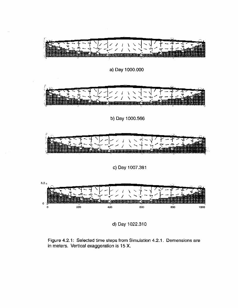
4.2.1 Extreme drought conditions

Figure 4.2.1 shows a simulation in which only one catotelm

layer, with a maximum depth of 6 m, is present. The acrotelm

is a constant 50 cm deep. After the system is allowed to reach

a stable state over the first 1000 days of the simulation, a

meteorological deficit of 1000 mm/yr is brought about, with

no apparent change in flow pattern for the rest of the

simulation (see Figure 4.2.1), even though hydraulic head at

47

\1 \

a) Day 1000.000

1 \ "1 \

b) Day 1000.566

c) Day 1007.381

J.r 1 ~

8.2::

200 400

i \

l "

600 800 1000

d) Day 1022.310

Figure 4.2.1: Selected time steps from Simulation 4.2.1. Demensions arein meters. Vertical exaggeration is 15 X.

the horizontal center of the bog (500 m mark) is changing

(decreasing) faster in the shallow part of the peat profile than

it is in the deep part. By Day 2000, the water table has been

lowered by about nineteen cm.

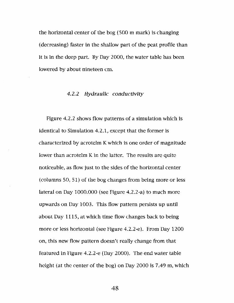
4.2.2 Hydraulic conductivity

Figure 4.2.2 shows flow patterns of a simulation which is

identical to Simulation 4.2.1, except that the former is

characterized by acrotelm K which is one order of magnitude

lower than acrotelm K in the latter. The results are quite

noticeable, as flow just to the sides of the horizontal center

(columns 50, 51) of the bog changes from being more or less

lateraion Day 1000.000 (see Figure 4.2.2-a) to much more

upwards on Day 1003. This flow pattern persists up until

about Day 1115, at which time flow changes back to being

more or less horizontal (see Figure 4.2.2-e). From Day 1200

on, this new flow pattern doesn't really change from that

featured in Figure 4.2.2-e (Day 2000). The end water table

height (at the center of the bog) on Day 2000 is 7.49 m, which

48

a) Day 1000.000

b) Day 1003.489

c) Day 1010.689

; \1 \.

d) Day 1115.683

o 200 400 600 800 1000

e) Day 2000.000

Figure 4.2.2: Selected time steps trom Simulation 4.2.2. Dimensions arein meters. Vertical exaggeration is 15 X.

translates into a drop of about 22 cm since the beginning of

the ldrought.'

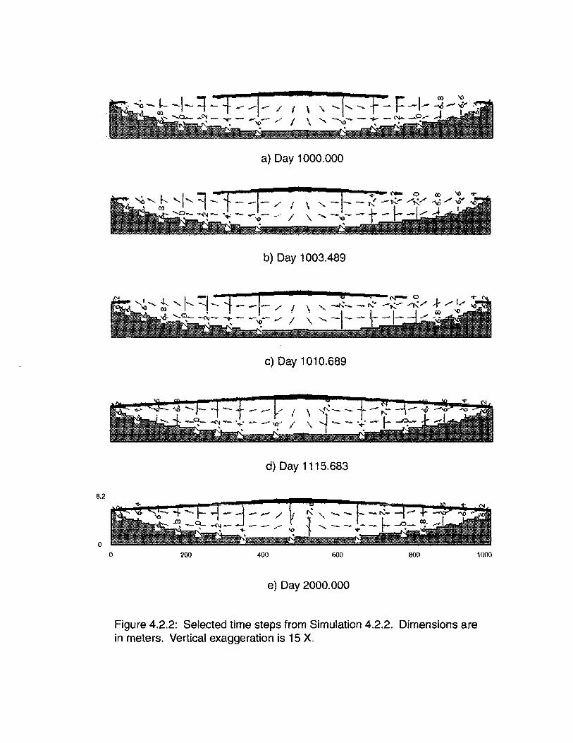
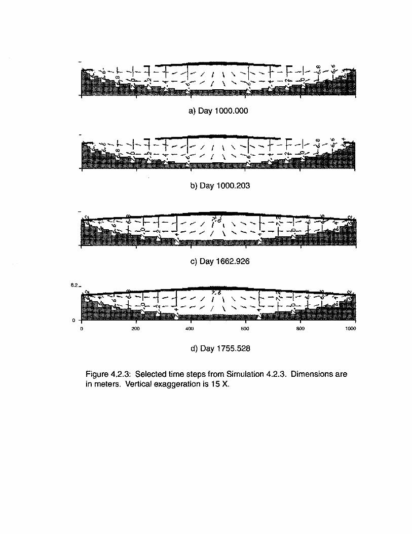
4.2.3 Drought severity variation

Figure 4.2.3 shows what happens when the precipitation

and evapotranspiration levels of Simulation 4.2.2's 'drought'

period are lowered to 800 mm/yr and 1400 mm/yr,

respectively. The resulting 600 mm/yr deficit results in the

same sort of flow patterns observed in Simulation 4.2.2 (see

Figures 4.2.2 and 4.2.3). Hydraulic head throughout the

system declines throughout the ldrought' stress period. (The

end water table elevation was 7.6 m, which is a drop of about

Il cm from the elevation at the beginning of the ldrought'.)

As head drops, horizontal flow just to the sides of column 51

changes to much more upward flow, as early as Day 1000.203

(see Figure 4.2.3-b). This pattern remains the same up until

about Day 1662, at which time flow here becomes horizontal

again.

49

a) Day 1000.000

-~-~ -1- i :-:r-l- / s, \S " -f' __ r- F-\- ~_f·1-'- -..0_ ~ - ""':' - -'D- /' 1 \" ~-- ~ "':' - ~ ~...- .J,

b) Day 1000.203

c) Day 1662.926

o 200 400 600 800 1000

d) Day 1755.528

Figure 4.2.3: Selected time steps trom Simulation 4.2.3. Dimensions arein meters. Vertical exaggeration is 15 X.

In Simulation 4.2.4, a water table drop of about only 2 cm

was effected (by setting precipitation to 920 mm/yr and

evapotranspiration to 1080 mm/yr) over the course of the

(drought' period. The resulting flow was indistinguishable

from that of Simulation 4.2.3 in terms of observable flow

pattern and flow pattern evolution. For this reason,

Simulation 4.2.4 does not have a fIgure.

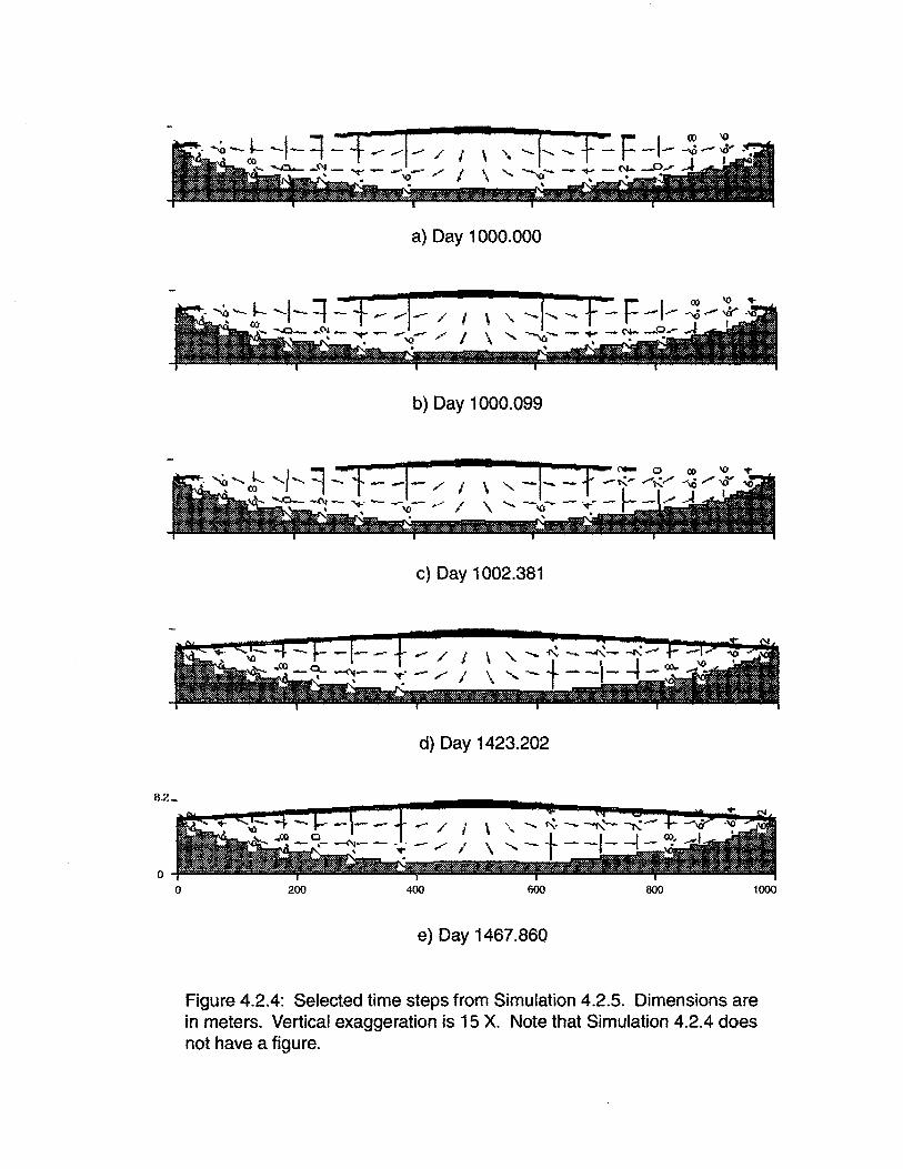
4.2.4 Porosity

In Simulation 4.2.5, porosity of the 50 cm acrotelm was

raised from 90 % to 95 %, and the porosity of the catotelm was

lowered from 90 % to 85 %. The meteorological deficit was

1000 mm/yr (600 mm/yr of precipitation minus 1600 mm/yr

of evapotranspiration). Although the flow 'reversaI' seems to

have begun slightly earlier than it did in Simulation 4.2.2, the

resulting flow patterns for the first 1423 days matched those

of the first 1423 days of Simulation 4.2.2, which had the same

meteorological deficit, but a porosity value of 90 % throughout

the entire domain. After Day 1423, however, Simulation 4.2.5

50

a) Day 1000.000

b) Day 1000.099

c) Day 1002.381

1 \1 \

d) Day 1423.202

o 200 400 600 800 1000

e) Day 1467.860

Figure 4.2.4: Selected time steps from Simulation 4.2.5. Dimensions arein meters. Vertical exaggeration is 15 X. Note that Simulation 4.2.4 doesnot have a figure.

differs in that flow returns to a more horizontal pattern (see

Figure 4.2.4-d). The water table drawdown ended up being

about 22 cm which matches the drawdown of Simulation 4.2.2.

Note that hydraulic head in the uppermost cell of column 51

increases slightly between Days 1423 and 1467, while head in

the column's lowermost cell decreases, thus showing the time

lag in pressure change transmission down the peat profile

which aIl simulations feature.

4.2.5 Discussion of KBT simulations

Because no KBT flow reversaI could be effected via

meteorological forcing of even an extreme nature (see next

paragraph), more emphasis was placed on determining how

altering substrate properties might influence, and perhaps

even bring about, flow reversais.

Even though there existed a Ume lag (see Simulation 4.2.1)

in head change between upper and Iower sections of the

domain -- the supposed driving factor behind gradient

reversais, also seen in the LRBT simulations -- no reversai

51

developed in any KBT simulation. The fact that reversaIs have

been observed in field KBTs (Devito et al., 1997) but not in the

simulations suggests that, as with the LRBT simulations,

parameterization was not sufficiently mimicked from the field.

As stated previously, it is possible that the distribution of

certain parameters such as hydraulic conductivity did not

match, in any simulation, real-world distribution of K.

Another possibility is that the morphology/topography of the

present study's KBT domains did not sufficiently match that of

Devito et al. (1997), for example.

Although no reversaIs could be obtained for KBT

simulations, a switch to more upwards-directed flow when

going from Simulation 4.2.1 to Simulation 4.2.2 suggests that

acrotelm hydraulic conductivity plays a role in KBT reversaIs.

The more upward-directed flow of Simulation 4.2.2 is similar

in pattern to the reversed flaw observed at Fraser's (1999) Mer

Bleue site, even though the former is a KBT and the latter a

LRBT. While Simulation 4.2.2 did nat praduce upward flow at

its horizontal center, it shauld be nated that the reversaI

52

observed at Mer Bleue, tao, did not occur at its horizontal

center.

Unexpectedly, lessening drought severity led ta longer­

lasting (reversais' (Le., upward-tending flow) -- likely a result

of the water table not dropping as far in the less severe

drought simulations (4.2.3,4.2.4). However, one might expect

more severe droughts to bring about longer lasting changes in

flow pattern, as occurred in the LRBT simulations. This brings

up the possibility that the KBT 'reversaIs' had nothing to do

with the time lag effect produced in both KBT and LRBT

simulations. The possibility exists that the bowl shape of KBT

systems has more to do with these switches to more upward­

tending flow than does the time lag effect. The testing of

various bowl shapes is beyond the scope of the present study.

While changing the porosity of both the acrotelm and the

catotelm (Simulation 4.2.5) seemed to have Httle effect on flow

pattern, it is reasonable to suggest that the quicker return to

horizontal flow exhibited by Simulation 4.2.5, as compared to

4.2.4, may be due to the acrotelm's slightly increased ability to

drain away water. The hypothesis that acrotelm K and

S3

porosity are more important, as regards flow reversaIs, than

corresponding catotelm properties is one that probably

favours K, as was shown previously.

Chapter 5.0 Summary and Conclusion

As observed in the field, hydraulic gradient reversaIs can

be significant in altering the chemistry of peatlands -­

particularly around the water table -- even when low hydraulic

gradients are involved (e.g., see Fraser, 1999, for an example

of dissoived organic carbon movement). Thus, aithough the

hydraulic gradients of the present study are even lower than

field-observed gradients, the importance of reversaIs should

not be overlooked. However, the effects of reversaIs on

peatland water storage and mass movement of water appear to

be limited, due to both the low hydraulic gradients involved

and the limited time during which reversaIs exist. Because of

this, their effects on both short-term peatland vegetation

change and long-term peatland evolution, for example, may be

limited. Still, the phenomenon of methane outgasing from

54

peatlands is of importance in the context of global climate

change, and appears ta require no more than a slight change

in flow pattern in arder ta occur. Thus, the dramatic reversals

produced in many of this study's simulations, and the

differences in their evolution, would appear ta be of some

significance in at least the dimate change context, even

though the timing of the simulated reversals differed from

those observed in the field. This thesis has shown that

meteorological deficit is required for the onset of hydraulic

gradient reversaIs, and it appears equally safe ta say that

larger droughts should be associated with longer-lasting flow

reversaIs in peatlands, and, therefore, possibly with larger

methane outgasing events. This thesis has shown that

hydraulic conductivity, too, plays a key role, though the

influence of catotelm division may not be as important ta

reversaIs (and outgasing) as once thought. It is hoped that,

with further work involving better parameterization -- perhaps

of a stochastic nature -- both simulated and observed flow

change (in response to meteorological and substrate forcing)

will come to match each other more closely. As the present

55

study was aimed more at discovering relative differences

between the effects of various forcing agents, rather than

matching field conditions exactly, its results should be viewed

accordingly.

S6

References

Anderson, M. and W. Woessner. 1992. Applied GroundwaterModeling. San Diego: Academie Press, Inc.

Chason, D. and D. Siegel. 1986. Hydraulic conductivity andrelated physical properties of peat, Lost River Peatland,northern Minnesota. Soil Science 142: 91-99.

Cheng, Xand M. P. Anderson. 1994. Simulating the influenceof lake position on groundwater fluxes. Water ResourcesResearch 30 (7): 2041-2049."

Davis, S. N. and R. j. M. De Wiest. 1966. Hydrogeology. NewYork: John Wiley & Sons Ine.

Devito, K. j., j. M. Waddington, and B. A. Branfireun. 1997.Flow reversaIs in peatlands influenced by local groundwatersystems. Hydrological Processes Il: 103-110.

Fetter, C. W. 1994. Apt!lied Hydrogeology Englewood Cliffs:Prentice Hall, Inc..

Fraser, C. J. D. 1999. The hydrology and dissolved organiccarbon (DOC) biogeochemistry in a boreal peatland. M.Se.thesis, McGiU University.

Freeze, A. and P. Witherspoon. 1967. Theoretical Analysis ofRegional Groundwater Flow; 2. Effeet of Water TableConfiguration and Subsurface Permeability Variation. WaterResources Research 3: 623-634.

Gafni, A. and K. N. Brooks. 1990. Hydraulic characteristics offour peatlands in Minnesota. Canadian Journal ofSoil Science70: 239-253.

Glaser, P., Wheeler, G., Gorham, E., and H. Wright. 1981. Thepatterned mires of the Red Lake Peatlands, northern

57

Minnesota: vegetation, water chemistry, and landforms.Journal ofEcology 69: 575-599.

Hemond, H. F. and J. C. Goldman. 1985. On non-Darcianwater flow in peat. Journal ofEcology 73: 579-584.

Hoag, R. and J. Priee. 1995. A field-scale, natural gradientsolute transport experiment in peat at a Newfoundlandblanket bog. Journal ofHydrology 172: 171-184.

Ingram, H. 1982. Size and shape in raised mire ecosystems: ageophysical model. Nature 297: 300-303.

Ingram, H. 1983. In Gore, A. (Ed.). Ecosystems of the World.Mires: Swamp1 Bog1Fen and Moor. General Studies. Vol. 4A.Amsterdam: Elsevier, pp. 67-158.

Ingram, H. and O. Bragg. 1984. The diplotelmic mire: Sornehydrological consequences reviewed. In Proceedings of the 7 th

International Feat Congress1Dublin1Vol. 1, pp. 220-234.

Ingram, H. 1991. Introduction to the ecohydrology of miresin the context of cultural perturbation. In Bragg, O., Hulme, P.,Ingram, H., and R. Robertson (Eds.) .. Peatland Ecosystems andMan: An Impact Assessment. British EcologicalSociety/International Peat Society, University of Dundee, pp.67-93.

Ivanov, K. E. 1981. Water Moyenient in Mirelands. London:Academic Press Inc..

Letts, M., Roulet, N., Corner, N., Verseghy, D., and M. Skarupa.1997. Parameterization of peatland hydraulic properties forthe Canadial1 Land Surface Scheme. Atmosphere-Oceal1 38:141-160.

McDonald, M. and A. Harbaugh. 1988. A modular three­dimensional finite-difference ground-water fIow mode!.Techniques of Water Resources Investigations OG-A1, D.S.Geological Survey.

58

McKenzie, J. 1997. Interactions between groundwater andwetlands in the Hudson Bay Lowlands. Honours thesis, McGillUniversity.

McNamara, J. P., D. 1. Siegel, P. H. Glaser, and R. M. Beek.1992. Hydrogeologie contraIs on peatland development in theMalloryville Wetland, New York (USA). Journal ofHydrology140: 279-296.

Mitsch, W. and J. Gosselink. 1993 we.tlands. New York: VanNostrand Reinhold.

Munter, J. and M. Anderson. 1981. The use of ground-waterfIow models for estimating lake seepage rates. Groundwater19: 608-616.

Reeve, A. S., Siegel, D. L, and P. H. Glaser. 2000. Simulatingvertical fIow in large peatlands. Journal ofHydrology 227:207-217.

Romanowicz, E. A., D. 1. Siegel, and P. H. Glaser. 1993.Hydraulic reversaIs and episodic methane emissions duringdrought cycles in mires. Geology 21: 231-234.

Siegel, D. I. 1981. Hydrogeologie setting of the Glacial LakeAgassiz Peatlands, northern Minnesota. V.S. Geological SurveyWater Resources Investigations, pp. 81-124.

Siegel, D. I. 1983. Ground water and the evolution ofpatterned mires, Glacial Lake Agassiz Peatlands, Minnesota.Journal ofEcology 71: 913-921.

Siegel, D. I. 1988. The Recharge-Discharge Function ofWetlands Near Juneau, Alaska: Part I. HydrogeologicalInvestigations. Ground Water 26 (4): 427-434.

Spitz, K. and J. Moreno. 1996. A Practical Guide taGroundwater and Solute Transport Modeling. New York: JohnWiley & Sons Ine.

59

Toth, J. 1963. A Theoretical Analysis of Groundwater Flow inSmall Drainage Basins. Journal ofGeophyysical Research 68:4795..4812.

Waddington, J. M. and N. T. Roulet. 1997. Groundwater flowand dissolved carbon movement in a boreal peatland. JournalofHydrology 191: 122-138.

Winter, T. 1978. Numerical Simulation of Steady State three­dirp.ensional Groundwater Flow Near Lakes. Water ResourcesRe$carch 14: 245-254.

'1

60