JOURNAL OF QUATERNARY SCIENCE (1995) 10 ( 1 ) 33-43 0 1995 by John Wiley & Sons, Ltd.

CCC 0267-81 79/95/01 0033-1 1

Modelling ice-sheet sensitivity to late Weichselian environments in the Sval bard-Barents Sea region M A R T I N J. SIECERT and JULIAN A. DOWDESWELL Centre for Glaciology, Institute of Earth Studies, University of Wales, Aberystwyth, Dyfed SY23 3DB, Wales

Siegert, M. j . and Dowdeswell, J. A. 1995. Modelling ice-sheet sensitivity to Late Weichselian environments in the Svalbard-Barents Sea region. /ournal of Quaternary Science, Vol 10, pp 3 3 4 3 . ISSN 0267-8179

Received 18 March 1994 Accepted 16 September 1994

ABSTRACT: Ice-proximal sedimentological features from the northwestern Barents Sea suggest that this region was covered by a grounded ice sheet during the Late Weichselian. However, there is debate as to whether these sediments were deposited by the ice sheet at its maximum or a retreating ice sheet that had covered the whole Barents Sea. To examine the likelihood of total glaciation of the Late Weichselian Barents Sea, a numerical ice-sheet model was run using a range of environmental conditions. Total glaciation of the Barents Sea, originating solely from Svalbard and the northwestern Barents Sea, was not predicted even under extreme environmental conditions. Therefore, if the Barents Sea was completely covered by a grounded Late Weichselian ice sheet, then a mechanism (not accounted for within the glaciological model) by which grounded ice could have formed rapidly within the central Barents Sea, may have been active during the last glaciation. Such mechanisms include (i) grounded ice migration from nearby ice sheets in Scandinavia and the central Barents Sea, (ii) the processes of sea-ice-induced ice-shelf thickening and (iii) isostatic uplift of the central Barents Sea floor.

Journal of Quaternary Science

KEYWORDS: Svalbard; Barents Sea; Late Weichselian; ice-sheet modelling.

Introduction and background

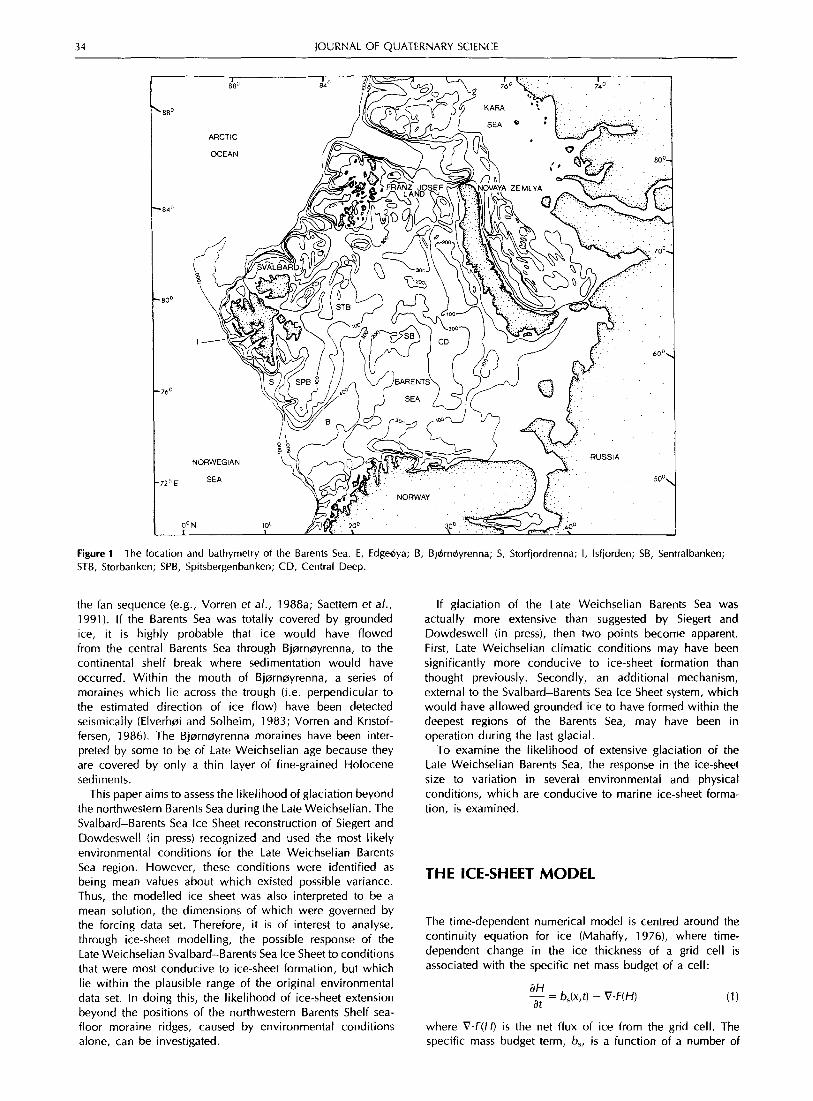
The Barents Sea, located to the north of mainland Norway and Russia between latitudes 72" and 84"N and longitudes 10" and 52"E (Fig. l), covering an area of 1.2 million km2, i s the largest epi-continental sea (Elverheri et a/., 1989). In the northwestern Barents Sea lies the island archipelago of Svalbard. Previous reconstructions of the ice sheet that occupied Svalbard and the Barents Sea during the Late Weichselian have ranged from total grounded ice coverage by a 2.5-km-thick ice sheet (e.g. Denton and Hughes, 1981) to an ice limit restricted to the coastal margins of Svalbard (e.g. Boulton, 1979). However, interpretation of recently obtained geological data from Svalbard and the Barents Sea has indicated that these two scenarios may be unlikely for the last full glacial.

Sedimentological information from Spitsbergenbanken (Fig. 2) indicates that the northwestern Barents Sea was covered by a grounded ice sheet during the Late Weichselian. On the floor of southern Spitsbergenbanken, glacially reworked sediments with a youngest age of 22000 radiocarbon years ago (yr BP) have been collected through shallow coring activities (Elverhpli et a/., 1993). These sediments indicate that by 22000 yr BP, Spitsbergenbanken was covered by grounded ice. The limit of this ice sheet can be estimated

from a series of sea-floor moraine ridges, flutes and ice- proximal sediment deposits that have been observed geophysi- cally (Fig. 2). These sedimentary features indicate that grounded glacier ice was located within the relatively shallow waters of the northwestern Barents Sea either at or after the Late Weichselian glacial maximum (Elverh~ii and Solheim, 1983; Elverhpli et a/., 1989). In addition, dated glacially derived sediments on the sea-floor of lsfjorden (Fig. 1) indicate that grounded ice, originating from Svalbard, reached up to the continental shelf break to the west of Spitsbergen during the Late Weichselian (Mangerud et a/., 1992). Glaciological modelling of the Late Weichselian Svalbard-Barents Sea Ice Sheet (Siegert and Dowdeswell, in press) has shown that, under likely Late Weichselian environmental conditions, the maximum extent of this ice sheet generally correlated well to the positions of sea-floor features within the northwestern Barents Sea (Fig. 2). However, this model did not deal with ice derived from Fennoscandia and the Kara Sea region (Fig. 1).

Glacigenic sediments and moraine ridges within Bjerm- plyrenna indicate that this trough has also been glaciated. Bjplrnplyrenna is the deepest trough within the western Barents Sea, and has an extensive glacigenic sedimentary fan at its mouth (Fig. 2). The geometry of Bjerrnplyrenna i s likely to derive from the action of an ice stream throughout a number of glaciations, which can be individually identified within

34 J O U R N A L OF Q U A T E R N A R Y SCIENCE

ARCTIC

OCEAN

Figure 1 STB, Storbanken; SPB, Spitsbergenbanken; CD, Central Deep.

The location and bathyrnetry of the Barents Sea. E, Edgedya; B, Bjdmdyrenna; S, Storfjordrenna; I, Isfjorden; SB, Sentralbanken;

the fan sequence (e.g., Vorren et a/., 1988a; Saettem et a/., 1991). If the Barents Sea was totally covered by grounded ice, it is highly probable that ice would have flowed from the central Barents Sea through Bjarnayrenna, to the continental shelf break where sedimentation would have occurred. Within the mouth of Bjarnayrenna, a series of moraines which lie across the trough (i.e. perpendicular to the estimated direction of ice flow) have been detected seismically (Elverh~ji and Solheim, 1983; Vorren and Kristof- fersen, 1986). The Bj~rnayrenna moraines have been inter- preted by some to be of Late Weichselian age because they are covered by only a thin layer of fine-grained Holocene sedi rnents.

This paper aims to assess the likelihood of glaciation beyond the northwestern Barents Sea during the Late Weichselian. The Svalbard-Barents Sea Ice Sheet reconstruction of Siegert and Dowdeswell (in press) recognized and used the most likely environmental conditions for the Late Weichselian Barents Sea region. However, these conditions were identified as being mean values about which existed possible variance. Thus, the modelled ice sheet was also interpreted to be a mean solution, the dimensions of which were governed by the forcing data set. Therefore, it is of interest to analyse, through ice-sheet modelling, the possible response of the Late Weichselian Svalbard-Barents Sea Ice Sheet to conditions that were most conducive to ice-sheet formation, but which lie within the plausible range of the original environmental data set. In doing this, the likelihood of ice-sheet extension beyond the positions of the northwestern Barents Shelf sea- floor moraine ridges, caused by environmental conditions alone, can be investigated.

If glaciation of the Late Weichselian Barents Sea was actually more extensive than suggested by Siegert and Dowdeswell (in press), then two points become apparent. First, Late Weichselian climatic conditions may have been significantly more conducive to ice-sheet formation than thought previously. Secondly, an additional mechanism, external to the Svalbard-Barents Sea Ice Sheet system, which would have allowed grounded ice to have formed within the deepest regions of the Barents Sea, may have been in operation during the last glacial.

To examine the likelihood of extensive glaciation of the Late Weichselian Barents Sea, the response in the ice-sheet size to variation in several environmental and physical conditions, which are conducive to marine ice-sheet forma- tion, is examined.

THE ICE-SHEET MODEL

The time-dependent numerical model is centred around the continuity equation for ice (Mahaffy, 1976), where time- dependent change in the ice thickness of a grid cell is associated with the specific net mass budget of a cell:

where V.F(H) i s the net flux of ice from the grid cell. The specific mass budget term, b,, is a function of a number of

ICE-SHEET MODELLING 35

r -Ice margin

Ice proximal deposits Acoustically transparent

uml EI lenses

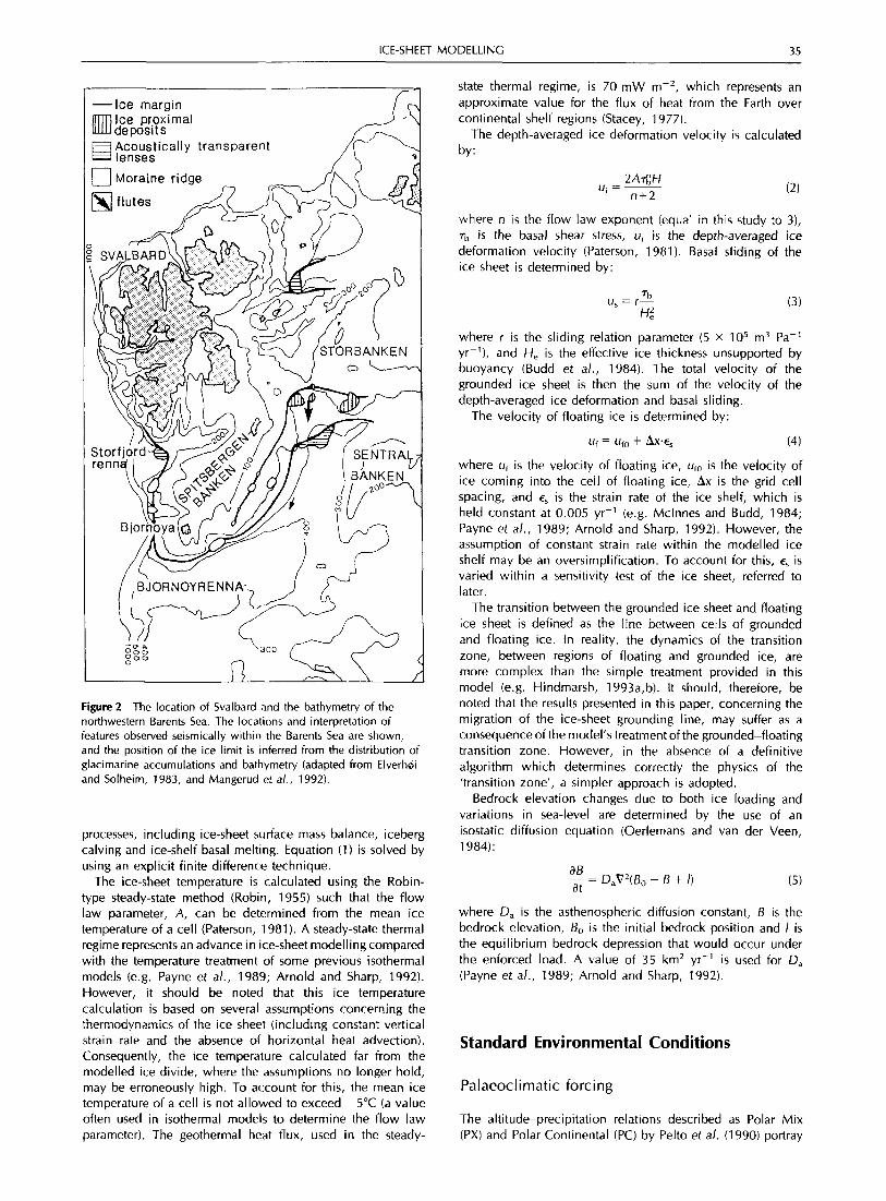
Figure 2 The location of Svalbard and the bathymetry of the northwestern Barents Sea. The locations and interpretation of features observed seismically within the Barents Sea are shown, and the position of the ice limit i s inferred from the distribution of glacimarine accumulations and bathymetry (adapted from Elverhdi and Solheim, 1983, and Mangerud et a/., 1992).

processes, including ice-sheet surface mass balance, iceberg calving and ice-shelf basal melting. Equation (1) is solved by using an explicit finite difference technique.

The ice-sheet temperature is calculated using the Robin- type steady-state method (Robin, 1955) such that the flow law parameter, A, can be determined from the mean ice temperature of a cell (Paterson, 1981). A steady-state thermal regime represents an advance in ice-sheet modelling compared with the temperature treatment of some previous isothermal models (e.g. Payne et a/., 1989; Arnold and Sharp, 1992). However, it should be noted that this ice temperature calculation i s based on several assumptions concerning the thermodynamics of the ice sheet (including constant vertical strain rate and the absence of horizontal heat advection). Consequently, the ice temperature calculated far from the modelled ice divide, where the assumptions no longer hold, may be erroneously high. To account for this, the mean ice temperature of a cell is not allowed to exceed -5°C (a value often used in isothermal models to determine the flow law parameter). The geothermal heat flux, used in the steady-

state thermal regime, is 70 mW m-2, which represents an approximate value for the flux of heat from the Earth over continental shelf regions (Stacey, 1977).

The depth-averaged ice deformation velocity is calculated by:

2A7”H u, = ~

n+2 12)

where n i s the flow law exponent (equal in this study to 3) , t-b i s the basal shear stress, ui i s the depth-averaged ice deformation velocity (Paterson, 1981). Basal sliding of the ice sheet i s determined by:

Tb u, = r- H:

( 3 )

where r is the sliding relation parameter (5 x lo5 m3 Pa-’ yr-‘1, and He is the effective ice thickness unsupported by buoyancy (Budd et a/., 1984). The total velocity of the grounded ice sheet i s then the sum of the velocity of the depth-averaged ice deformation and basal sliding.

The velocity of floating ice is determined by:

~f = Ufo + AX.€, 14)

where uf i s the velocity of floating ice, ufo i s the velocity of ice coming into the cell of floating ice, Ax i s the grid cell spacing, and E , i s the strain rate of the ice shelf, which is held constant at 0.005 yr-l (e.g. Mclnnes and Budd, 1984; Payne et a/ . , 1989; Arnold and Sharp, 1992). However, the assumption of constant strain rate within the modelled ice shelf may be an oversimplification. To account for this, es is varied within a sensitivity test of the ice sheet, referred to later.

The transition between the grounded ice sheet and floating ice sheet is defined as the line between cells of grounded and floating ice. In reality, the dynamics of the transition zone, between regions of floating and grounded ice, are more complex than the simple treatment provided in this model (e.g. Hindmarsh, 1993a,b). It should, therefore, be noted that the results presented in this paper, concerning the migration of the ice-sheet grounding line, may suffer as a consequence of the model’s treatment of the grounded-floating transition zone. However, in the absence of a definitive algorithm which determines correctly the physics of the ‘transition zone’, a simpler approach is adopted.

Bedrock elevation changes due to both ice loading and variations in sea-level are determined by the use of an isostatic diffusion equation (Oerlemans and van der Veen, 1984):

aB at - = D,V2(Bo - B + /) (5)

where D, i s the asthenospheric diffusion constant, B is the bedrock elevation, Bo is the initial bedrock position and I i s the equilibrium bedrock depression that would occur under the enforced load. A value of 35 km2 yr-’ i s used for D, (Payne et a/., 1989; Arnold and Sharp, 1992).

Standard Environmental Conditions

Palaeocl i matic forc i ng

The altitude-precipitation relations described as Polar Mix (PX) and Polar Continental (PC) by Pelto eta/. (1990) portray

36 JOURNAL OF QUATERNARY SCIENCE

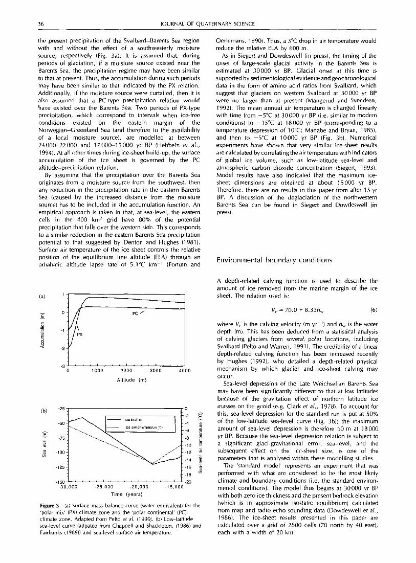
the present precipitation of the Svalbard-Barents Sea region with and without the effect of a southwesterly moisture source, respectively (Fig. 3a). It is assumed that, during periods of glaciation, if a moisture source existed near the Barents Sea, the precipitation regime may have been similar to that at present. Thus, the accumulation during such periods may have been similar to that indicated by the PX relation. Additionally, if the moisture source were curtailed, then it i s also assumed that a PC-type precipitation relation would have existed over the Barents Sea. Two periods of PX-type precipitation, which correspond to intervals when ice-free conditions existed on the eastern margin of the Norwegian-Greenland Sea (and therefore to the availability of a local moisture source), are modelled at between 24000-22000 and 170OCLl5000 yr BP (Hebbeln et a/., 1994). At all other times during ice-sheet build-up, the surface accumulation of the ice sheet i s governed by the PC altitude-precipitation relation.

By assuming that the precipitation over the Barents Sea originates from a moisture source from the southwest, then any reduction in the precipitation rate in the eastern Barents Sea (caused by the increased distance from the moisture source) has to be included in the accumulation function. An empirical approach is taken in that, at sea-level, the eastern cells in the 400 km2 grid have 80% of the potential precipitation that falls over the western side. This corresponds to a similar reduction in the eastern Barents Sea precipitation potential to that suggested by Denton and Hughes (1981). Surface air temperature of the ice sheet controls the relative position of the equilibrium line altitude (ELA) through an adiabatic altitude lapse rate of 5.1"C km-' (Fortuin and

Fc'

' . ' ' l ' . . ' ' . ' 0 1 0 0 0 2000 3000 4000

Altitude (in)

-25 I I-0

sea-level air temperature ('C)

-125 - --16 $

-150 -20 ' " " ' " ' I " ' ' I 1-18 rn

-30,000 -25,000 -20,000 -15,000

Time (years)

Figure 3 'polar mix' (PX) climate zone and the 'polar continental' (PC) climate zone. Adapted from Pelto et a/. (1 990). (b) Low-latitude sea-level curve (adpated from Chappell and Shackleton, (1986) and Fairbanks ( 1 989)) and sea-level surface air temperature.

(a) Surface mass balance curve (water equivalent) for the

Oerlemans, 1990). Thus, a 3°C drop in air temperature would reduce the relative ELA by 600 m.

As in Siegert and Dowdeswell (in press), the timing of the onset of large-scale glacial activity in the Barents Sea i s estimated at 30000 yr BP. Glacial onset at this time i s supported by sedimentological evidence and geochronological data in the form of amino acid ratios from Svalbard, which suggest that glaciers on western Svalbard at 30000 yr BP were no larger than at present (Mangerud and Svendsen, 1992). The mean annual air temperature i s changed linearly with time from -5°C at 30000 yr BP (i.e. similar to modern conditions) to -15°C at 18000 yr BP (corresponding to a temperature depression of 10°C; Manabe and Bryan, 1985), and then to -5°C at 10000 yr BP (Fig. 3b). Numerical experiments have shown that very similar ice-sheet results are calculated by correlating the air temperature with indicators of global ice volume, such as low-latitude sea-level and atmospheric carbon dioxide concentration (Siegert, 1993). Model results have also indicated that the maximum ice- sheet dimensions are obtained at about 15000 yr BP. Therefore, there are no results in this paper from after 15 yr BP. A discussion of the deglaciation of the northwestern Barents Sea can be found in Siegert and Dowdeswell (in press).

Environmental boundary conditions

A depth-related calving function is used to describe the amount of ice removed from the marine margin of the ice sheet. The relation used is:

V, = 70.0 + 8.33hW (6)

where V, i s the calving velocity (m yr-') and h, is the water depth (m). This has been deduced from a statistical analysis of calving glaciers from several polar locations, including Svalbard (Pelto and Warren, 1991). The credibility of a linear depth-related calving function has been increased recently by Hughes (1992), who detailed a depth-related physical mechanism by which glacier and ice-sheet calving may occur.

Sea-level depression of the Late Weichselian Barents Sea may have been significantly different to that at low latitudes because of the gravitation effect of northern latitude ice masses on the geoid (e.g. Clark et a/., 1978). To account for this, sea-level depression for the standard run i s put at 50% of the low-latitude sea-level curve (Fig. 3b); the maximum amount of sea-level depression i s therefore 60 m at 18000 yr BP. Because the sea-level depression relation is subject to a significant glaci-gravitational error, sea-level, and the subsequent effect on the ice-sheet size, is one of the parameters that i s analysed within these modelling studies.

The 'standard model' represents an experiment that was performed with what are considered to be the most likely climate and boundary conditions (i.e. the standard environ- mental conditions). The model thus begins at 30000 yr BP with both zero ice thickness and the present bedrock elevation (which i s in approximate isostatic equilibrium) calculated from map and radio echo sounding data (Dowdeswell et a/., 1986). The ice-sheet results presented in this paper are calculated over a grid of 2800 cells (70 north by 40 east), each with a width of 20 km.

ICE-SHEET MODELLING 37

Standard model results

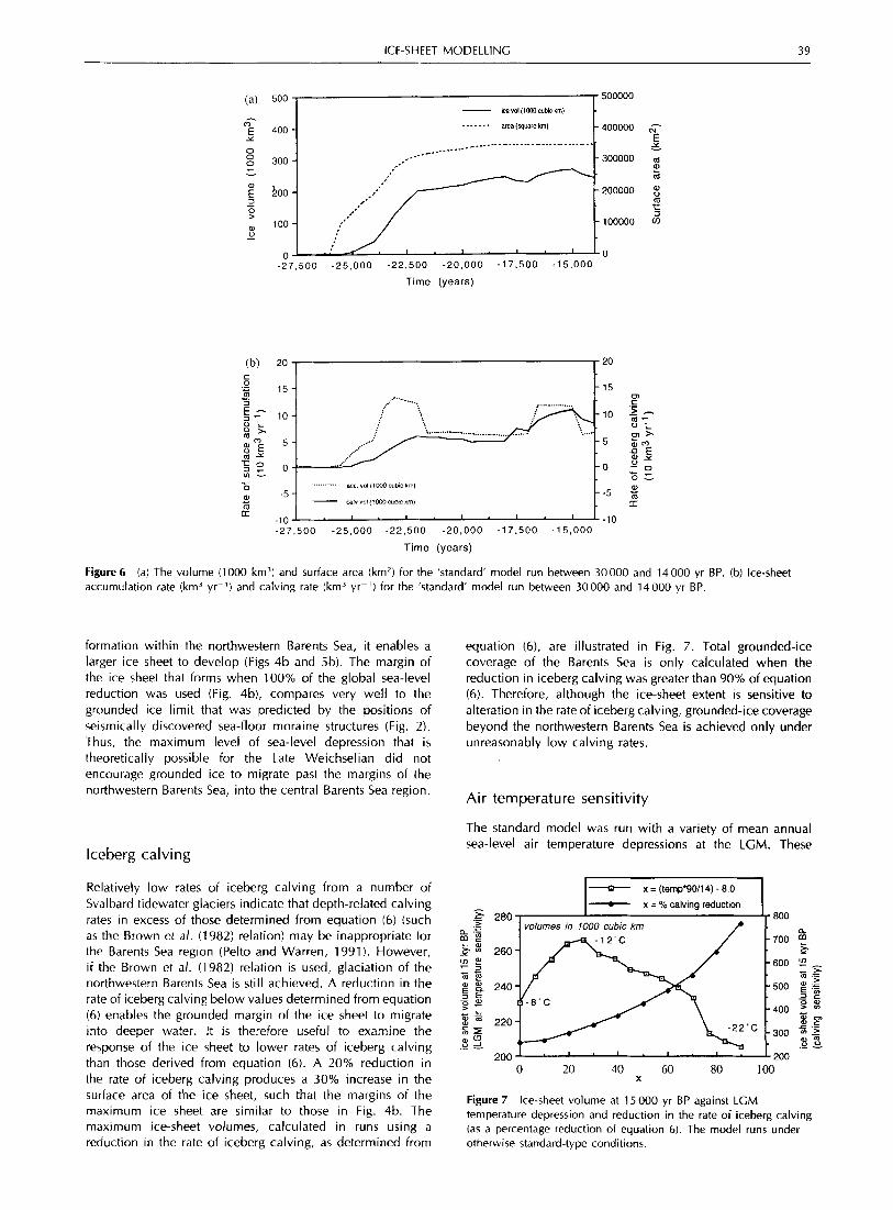
The standard model reconstruction formed an initial ice sheet by accumulating ice over Svalbard shortly before 25000 yr BP, which during the succeeding 5000 yr spread over the neighbouring shallow sea on to Spitsbergenbanken (Fig. 1). Subsequently, the northwestern Barents Sea became covered by a grounded ice sheet by 20000 yr BP. At 15000 yr BP the ice sheet had grown to near its maximum size. This ice sheet has a maximum thickness of about 1300 m, located around Edgeraya (Fig. 4a). The surface elevation of the ice sheet at 15 000 yr BP was governed largely by the underlying bedrock elevation (Fig. Sa), such that the topography of Svalbard can be clearly seen within the surface of the ice sheet. Consequently, the drainage divides and flowlines of

~~ ~ ~

the ice sheet were controlled by the existing fjords and troughs of Svalbard and the northwestern Barents Sea. The maximum ice sheet occupied only the northwestern Barents Sea. Thus, total grounded ice coverage of the Barents Sea was not attained in the standard model run. The variation in ice volume, surface area and mass balance terms with time are given in Fig. 6.

Because the standard model's forcing data are a 'most likely' prediction, they are therefore subject to a variance about these values. It is therefore necessary that a series of sensitivity experiments be made (where all other variables are held constant), which account for the possible variability within the standard model forcing data. The particular data that are varied within the sensitivity examinations are those that are most likely to affect the ice-sheet evolution through a glacial cycle. Thus, the environmental and physical

ICE THICKNESS

(a) Standard model

(c) PX accumulation between 1 I 24 and 18 kyr BP

'b) Sea level depression = 120m

(d) PC accumulation PX accumulation

I

Figure 4 Ice thickness (contours in 200 m intervals) at 15000 yr BP. (a) Standard model. (b) Sea-level depression of 120 rn at the LCM. (c) PX-type accumulation between 24000 and 18000 yr BP. (d) PC-type accumulation only. (e) PX-type accumulation only, with the model run under otherwise constant LCM type conditions until mass balance stability had been achieved. The Svalbard archipelago and the 400 m bathymetric contour are shown as an aid to location.

38 JOURNAL OF QUATERNARY SCIENCE

SURFACE ELEVATION

(b) Sea level depression

e) Stable ice sheet under

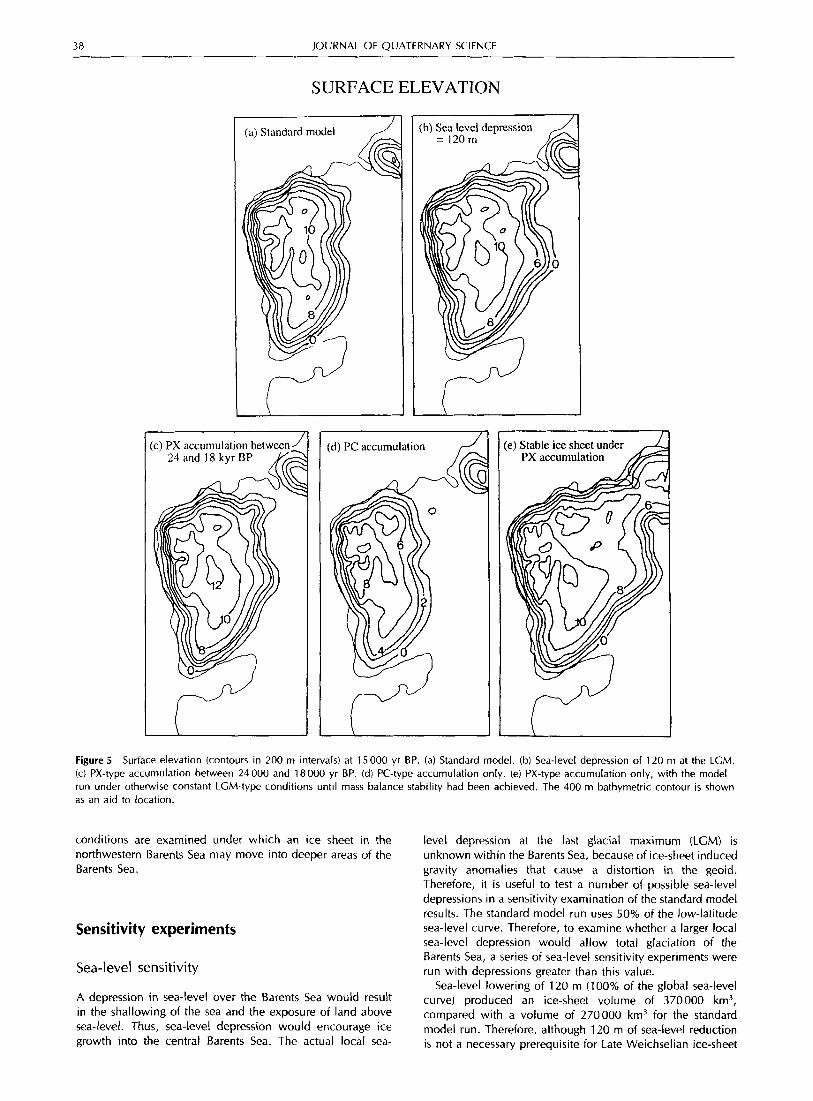
Figure 5 Surface elevation (contours in 200 m intervals) at 15000 yr BP. (a) Standard model. (b) Sea-level depression of 120 m at the LGM. (c) PX-type accumulation between 24 000 and 18 000 yr BP. (d) PC-type accumulation only. (e) PX-type accumulation only, with the model run under otherwise constant LGM-type conditions until mass balance stability had been achieved. The 400 m bathymetric contour is shown as an aid to location.

conditions are examined under which an ice sheet in the northwestern Barents Sea may move into deeper areas of the Barents Sea.

Sensitivity experiments

Sea-level sensitivity

A depression in sea-level over the Barents Sea would result in the shallowing of the sea and the exposure of land above sea-level. Thus, sea-level depression would encourage ice growth into the central Barents Sea. The actual local sea-

level depression at the last glacial maximum (LGM) is unknown within the Barents Sea, because of ice-sheet induced gravity anomalies that cause a distortion in the geoid. Therefore, it i s useful to test a number of possible sea-level depressions in a sensitivity examination of the standard model results. The standard model run uses 50% of the low-latitude sea-level curve. Therefore, to examine whether a larger local sea-level depression would allow total glaciation of the Barents Sea, a series of sea-level sensitivity experiments were run with depressions greater than this value.

Sea-level lowering of 120 m (100% of the global sea-level curve) produced an ice-sheet volume of 370000 km3, compared with a volume of 270000 km3 for the standard model run. Therefore, although 120 rn of sea-level reduction is not a necessary prerequisite for Late Weichselian ice-sheet

ICE-SHEET MODELLING 39

1 m E 400 - Y

0 8 300 - 7 .-, #

0

100 -

a, 100-

- 5 U -

0

500000 (a) 500 - lcevol LIWO cubic km)

area ( w a r e bn) -400000 &j- . -. . . -

E 5

-300000 m L

-200000 2

_ _ _ _ _ _ _-_ ~ __. ..-.-- ._--- *-

m r - 100000 0

1 . 1 . 1 0

15

L . . . .. . ..... . ace “01 (1wO Cubic kml

- cab wl(fDweublc km) - -5 -5 -

I . , , . , . I -10 -10 -27,500 -25,000 -22,500 -20,000 -17.500 -1 5,000

Time (years)

Figure 6 accumulation rate (km3 yr-I) and calving rate (km3 yrr’) for the ‘standard‘ model run between 30000 and 14000 yr BP.

(a) The volume (1000 km3) and surface area (km2) for the ’standard’ model run between 30000 and 14000 yr BP. (b) Ice-sheet

formation within the northwestern Barents Sea, it enables a larger ice sheet to develop (Figs 4b and 5b). The margin of the ice sheet that forms when 100% of the global sea-level reduction was used (Fig. 4b), compares very well to the grounded ice limit that was predicted by the positions of seismically discovered sea-floor moraine structures (Fig. 2). Thus, the maximum level of sea-level depression that is theoretically possible for the Late Weichselian did not encourage grounded ice to migrate past the margins of the northwestern Barents Sea, into the central Barents Sea region.

Iceberg calving

Relatively low rates of iceberg calving from a number of Svalbard tidewater glaciers indicate that depth-related calving rates in excess of those determined from equation (6) (such as the Brown et a / . (1982) relation) may be inappropriate for the Barents Sea region (Pelto and Warren, 1991). However, if the Brown et a/. (1982) relation is used, glaciation of the northwestern Barents Sea is still achieved. A reduction in the rate of iceberg calving below values determined from equation (6) enables the grounded margin of the ice sheet to migrate into deeper water. It i s therefore useful to examine the response of the ice sheet to lower rates of iceberg calving than those derived from equation (6). A 20% reduction in the rate of iceberg calving produces a 30% increase in the surface area of the ice sheet, such that the margins of the maximum ice sheet are similar to those in Fig. 4b. The maximum ice-sheet volumes, calculated in runs using a reduction in the rate of iceberg calving, as determined from

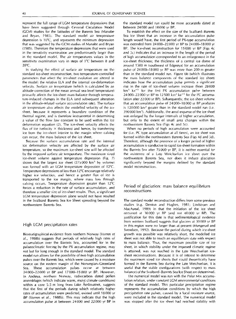
equation (6) , are illustrated in Fig. 7. Total grounded-ice coverage of the Barents Sea i s only calculated when the reduction in iceberg calving was greater than 90% of equation (6). Therefore, although the ice-sheet extent is sensitive to alteration in the rate of iceberg calving, grounded-ice coverage beyond the northwestern Barents Sea i s achieved only under unreasonably low calving rates.

Air temperature sensitivity

The standard model was run with a variety of mean annual sea-level air temperature depressions at the LGM. These

x = (temp’90/14) - 8.0 x = % calving reduction

280 volumes in 1000 cubic km

- 500

0 20 60 80 100 40 x

Figure 7 Ice-sheet volume at 15 000 yr BP against LGM temperature depression and reduction in the rate of iceberg calving (as a percentage reduction of equation 6). The model runs under otherwise standard-type conditions.

40 JOURNAL OF QUATERNARY SCIENCE

represent the full range of LGM temperature depressions that have been suggested through General Circulation Model (GCM) studies for the latitudes of the Barents Sea (Manabe and Bryan, 1985). The standard model air temperature depression i s 10°C, and represents the minimum depression that was suggested by the GCM studies of Manabe and Bryan (1 985). Therefore the temperature depressions that were used in the sensitivity examination are predominantly larger than in the standard model. The air temperatures values in the sensitivity examination vary in steps of 1°C between 8 and 20°C.

In studying the effect of surface air temperature on the standard ice-sheet reconstruction, two temperature-controlled parameters that affect the ice-sheet evolution are altered in the model: the relative ELA and the internal ice-deformation velocity. Surface air temperature (which is calculated by an altitude correction of the mean annual sea-level temperature) primarily affects the ice-sheet mass balance through tempera- ture-induced changes in the ELA (and subsequent alteration in the altitude-related surface accumulation rate). The surface air temperature also affects the modelled velocity of the ice sheet, because it represents a boundary condition of the thermal regime, and is therefore instrumental in determining a value of the flow law constant to be used within the ice deformation equation (2). The ice-sheet velocity affects the flux of ice (velocity x thickness) and hence, by transferring ice from the ice-sheet interior to the margin where calving can occur, the mass balance of the ice sheet.

Because the surface accumulation rate and the internal ice deformation velocity are affected by the surface air temperature, so the maximum ice-sheet size wil l be affected by the imposed surface air temperature. The maximum sized ice-sheet volume against temperature depression (Fig. 7 ) shows that the largest ice sheet (275000 km3 by volume) was formed with an LGM temperature depression of 12°C. Temperature depressions of less than 1 2°C encourage relatively higher ice velocities, and hence a greater flux of ice is transported to the ice margin, where mass loss through calving occurs. Temperature depression greater than 12°C forces a reduction in the rate of surface accumulation, and therefore a smaller size of ice-sheet results. Thus, a significant LGM temperature depression alone would not have resulted in the Svalbard-Barents Sea Ice Sheet spreading beyond the northwestern Barents Sea.

High LGM precipitation rates

Biostratigraphical evidence from northern Norway (Vorren et a/., 1988b) suggests that periods of relatively high rates of accumulation over the Barents Sea, accounted for in the palaeoclimatic forcing by the PX accumulation regime, may not last for long enough in the standard model. The standard model run allows for the possibility of two high accumulation pulses over the Barents Sea, which were caused by a moisture source on the eastern margin of the Norwegian-Greenland Sea. These accumulation pulses occur at between 24000-22000 yr BP and 17OOCb15000 yr BP. However, in Andraya, northern Norway, radiocarbon dated pollen assemblages (which indicate warm, moist climate conditions) within a core 5.5 m long from Lake Aer:svatnet, suggests that the first of the periods during which relatively higher rates of accumulation were predicted, existed until 18 000 yr BP (Vorren et a/., 198813). This may indicate that the high accumulation pulse at between 24000 and 22000 yr BP in

the standard model run could be more accurately dated at between 24 000 and 18 000 yr BP.

To establish the effect on the size of the Svalbard-Barents Sea Ice Sheet that an increase in the accumulation pulse length would have, the first period of PX-type accumulation was extended from 24 000-22 000 yr BP to 24 00&18 000 yr BP. The ice-sheet reconstruction for 15 000 yr BP (Figs 4c and 5c) indicates that an increase in the length of the period of high accumulation corresponded to an enlargement in the ice-sheet thickness; the thickness of a central ice dome of around 1500 m (southwest of Edgeerya) for an accumulation pulse of 24 000-18 000 yr BP was more than 200 m greater than in the standard model run. Figure 6b (which illustrates the mass balance components of the standard ice sheet) indicates how the accumulation pulse permits a significant rise in the rate of ice-sheet volume increase (from 28000 km3 ka-’ for the first PX accumulation pulse between 24000-22000 yr BP to 12 500 km’ ka-’ for the PC accumu- lation after 22 000 yr BP). Subsequently, the ice-sheet volume that an accumulation pulse of 24 000-1 8 000 yr BP produces i s 120000 km3 greater than in the standard model run (i.e. 390000 km’). Additionally, the areal expanse of the ice sheet was enlarged by the longer intervals of higher accumulation, but only to the extent of small area changes within the northwestern Barents Sea (Figs 4c and Sc).

When no periods of high accumulation were accounted for (i.e. PC type accumulation at all times), an ice sheet was formed within the northwestern Barents Sea (Figs 4d and 5d). Therefore, although the presence of a longer period of higher accumulation is conducive to rapid ice-sheet formation within the Barents Sea after 25000 yr BP, it i s neither essential for the existence of a Late Weichselian ice sheet over the northwestern Barents Sea, nor does it induce glaciation significantly beyond the margins defined by the standard model reconstruction.

Period of glaciation: mass balance equilibrium reconstructions

The standard model reconstruction differs from some previous studies (e.g. Denton and Hughes, 1981; Lindstrom and MacAyeal, 1989) in that the initiation of the ice sheet occurred at 30000 yr BP (and not 40000 yr BP). The justification for this date is that sedimentological evidence from western Svalbard suggests that glaciers at 30000 yr BP in this region were no larger than at present (Mangerud and Svendsen, 1992). Because the period during which ice-sheet growth was possible was relatively short, the modelled ice sheet was not able to reach an equilibrium state with respect to mass balance. Thus, the maximum possible size of ice sheet, in which stability under the imposed climatic regime is attained, was not reached in the Late Weichselian ice- sheet reconstructions. Because it is of interest to determine the maximum sized ice sheets that could theoretically have formed in the Barents Sea during the Late Weichselian, it is useful that the stable configurations (with respect to mass balance) of the Svalbard-Barents Sea Ice Sheet are determined.

The numerical model was run with the Polar Mix accumu- lation relation, under constant LGM environmental conditions of the standard model. This particular precipitation regime represents the accumulation conditions by which the high precipitation rate pulses, caused by a local moisture source, were included in the standard model. The numerical model was stopped after the ice sheet had reached stability with

ICE-SHEET MODELLING 41

respect to mass balance. This happened shortly after 10000 yr of model running time.

The Polar Mix stable ice sheet has a maximum thickness of around 1800 m, located to the east of Edgenya (Figs 4e and 5e), and a volume of 565 000 km3. This ice sheet exceeds the volume (270000 km3) and maximum thickness (1 300 m) of the standard ice sheet (Fig. 4a). However, the most important feature of the equilibrium ice sheet under the highest rate of precipitation conditions is that the ice sheet st i l l fails to cover the entire Barents Sea, even though the ice mass now coalesces with that of Franz Josef Land to the east (Fig. 1, Figs 4e and 5e). Thus, the maximum possible size of ice sheet that i s predicted in these sensitivity exercises did not cause the margin of the Late Weichselian Svalbard-Barents Sea Ice Sheet to migrate past the position of sea-floor moraine structures of the northwestern Barents Sea (Figs 2 and 4e).

Ice-shelf strain rate sensitivity

The dynamics of ice shelves are, in reality, more complex than those used in the numerical model. Specifically, the assumption that the strain rate of the ice shelf, E,, remains constant at 0.005 yr-’, may be too simple. To examine how this simplification affects the standard model results, an ice sheet sensitivity examination was performed by varying the value of eS between 0.00025 and 0.05 yr-’. The maximum variation in the ice-sheet volume at 15000 yr BP, from that determined in the standard model run (270000 km3), caused by an alteration in the ice-shelf strain rate was calculated to be less than 500 km3. Prior to 15 000 yr BP during ice-sheet build-up, grounded ice spread on to the northwestern Barents Sea floor by the migration of the grounding line from the Svalbard archipelago. In the standard model during this period, the action of floating ice did not greatly contribute to the spreading of the grounded ice mass (i.e. there were no large ice shelves formed and therefore no regions of the ice sheet formed by the regrounding of the floating ice). The modelled ice sheet at 15000 yr BP (Fig. 4a) has very few areas of floating ice, represented by only a few cells at the ice-sheet margin. Subsequently, a change in the ice-shelf strain rate parameter induces alterations in the modelled dynamics over a relatively small percentage of the total ice sheet in the northwestern Barents Sea at 15000 yr BP. Thus, a variation in the ice-shelf strain rate produced little alteration to, firstly, the growth of the ice sheet and, secondly, the dynamics of the maximum sized ice sheet as detailed in the standard model. Therefore, the modelled ice sheet was observed to be stable to variations in the ice-shelf strain rate.

Discussion

The results from this sensitivity exercise indicate that even under environmental conditions most conducive to grounded- ice formation (yet still plausible for the Late Weichselian), total glaciation of the Barents Sea, initiating from Svalbard, has not been predicted. To enable grounded ice to be modelled within the deeper regions of the Barents Sea, either rates of surface accumulation in excess of that of present-day Svalbard must be used or the local sea-level depression must be adjusted to over 200 m. Neither of these two ways of forming ice into the central Barents Sea are plausible for the Late Weichselian. Thus, if grounded ice was present over

deeper regions of the Late Weichselian Barents Sea, the expansion of the grounded-ice margin was not a direct ice- sheet response of the Svalbard-Barents Sea Ice Sheet to the environmental conditions. Therefore, for grounded ice to exist within deeper regions of the Barents Sea, a mechanism external to the Svalbard-Barents Sea Ice Sheet system, which has not been included in the numerical model, must be accounted for.

The maximum sized ice sheets predicted by the sensitivity experiments did not cover Bj~rnnyrenna and the southern Barents Sea (Figs 4 and 5). However, glacigenic sediments and geophysically observed moraines within Bjerrn~yrenna indicate that the trough may have been covered by grounded ice during the Late Weichselian (Vorren and Kristoffersen, 1986). It should be emphasised that, because our model does not account for ice sheets in either Scandinavia or the central Barents Sea, we cannot rule out the possibility of ice input to the southern Barents Sea from areas other than the northwestern Barents Sea.

An ice shelf within the central Barents Sea

One theory by which grounded ice within the Late Weichselian central Barents Sea may have formed is that permanent sea ice, which was held fast within the Barents Sea, thickened, owing to surface accumulation and low rates of basal melting, to form an ice shelf which eventually grounded over the entire Barents Shelf region (e.g. Denton and Hughes, 1981; Hughes, 1987). This ice shelf may also have acted to suppress the calving of icebergs from the grounded margin of the ice sheet in the northwestern Barents Sea into the more central regions. Unfortunately, because the formation of a sea-ice- induced ice shelf i s purely theoretical, the conditions required for its formation are poorly understood. We do not, therefore, provide any numerical results on the formation and growth of a sea-ice-induced Late Weichselian Barents Sea Ice Shelf. However, in the light of recent palaeoceanographic data from the Norwegian and southwestern Barents seas, a qualitative discussion of the problem i s provided.

If an ice shelf did form within the Late Weichselian Barents Sea, the mass balance of the proposed ice shelf would be, as in Antarctic ice shelves, largely controlled by surface accumulation and basal melting/freezing. The basal boundary condition of modern ice shelves has been shown to be related to both the thermal conductivity of the ice and the thermal character of the neighbouring seas (because it is these seas that provide the thermal input, through oceanic flow, beneath the ice shelf). Consequently, to estimate the melting potential of the Barents Sea during the Late Weichselian, the thermal character of the Norwegian-Greenland Sea should be con- sidered. During times of permanent sea-ice coverage within the Norwegian-Greenland Sea, due to the lack of relatively warm water from the North Atlantic entering the Barents Sea via the Norwegian and North Cape currents (Hisdal, 1985), it is likely that the Barents Sea was sufficiently cold that ice melting would have been relatively low. Conversely, during periods of ice-free conditions within the eastern Norwegian-Greenland Sea, the potential melting of fast ice within the Barents Sea would be considerably enhanced due to the input of relatively warm waters from the North Atlantic. When the seas surrounding an ice shelf are only seasonally covered by sea ice, the basal melt rate has been recorded to be generally higher than 0.5 m yr-‘ (e.g. the George VI Ice

42 JOURNAL OF QUATERNARY SCIENCE

Shelf has a basal melt rate of 2 m yr-’; Bishop and Walton, 1981). Because the eastern margin of the Norwegian-Greenland Sea was ice-free at between at least 24000-1 8 000 yr BP and 17 000-1 5 000 yr BP (e.g. Hebbeln et a / . , 1994), the basal melt rate potential within the Barents Sea during these periods may have been above 0.5 m yr-’. Therefore, if an ice shelf existed in the Late Weichselian Barents Sea it may have been subject to considerably higher rates of basal melting than accumulation rates on Svalbard at present. Thus, Svalbard-Barents Sea Ice Sheet reconstructions which initiate from a sea-ice-induced ice shelf may not be appropriate for the last glacial (although they may have been for preceding glaciations).

Equilibrium ice-sheet reconstructions, where the model runs for over 20000 yr and iceberg calving within the central Barents Sea is curtailed, have produced an ice sheet very similar in thickness to the Denton and Hughes prediction (Siegert, 1993). Given that sedimentological evidence from Svalbard and Spitsbergenbanken suggests that glaciers on western Svalbard at 30000 yr BP were no larger than at present and that ice build-up within the Barents Sea occurred after 25000 yr BP (Hald et a/., 1990; Elverheri et a/., 1992; Mangerud et a/. , 1992), a 2.5-km-thick ice sheet i s unlikely to have existed within the Late Weichselian Barents Sea. An alternative scenario is, of course, that ice build-up began significantly earlier than 30000 yr BP, which would require a reinterpretation of the geochronological evidence for the inception of full glacial conditions during the Late Weichselian in Svalbard (cf. Mangerud and Svendsen, 1992).

isostatic uplift within the central Barents Sea

If the Late Weichselian Barents Sea could not sustain a sea- ice-induced ice shelf, and grounded ice did exist within Bjerrneryrenna at the LGM, then a method of glaciation, other than ice spreading from nearby ice sheets or a sea-ice- induced ice shelf, must be acknowledged.

One possible mechanism of grounded-ice formation that i s currently being investigated i s the isostatic uplift of Sentralbanken (a shallow bank within the central Barents Sea) above sea-level during the last ice age. Sentralbanken is located in the central Barents Sea (Fig. l ) , and represents an area where no ice was predicted to have existed by the standard model. This uplift may have been caused by an isostatic forebulge from the Svalbard, Fennoscandian and Kara Sea ice sheets (Fjeldskaar and Elverheri, pers. comm.). If Sentralbanken was uplifted above sea-level, then an ice- cap would have readily formed over it. The emergence of Sentralbanken may have produced a chain of grounded ice- domes from Svalbard to Scandinavia, which surrounded Bjerrneryrenna. Therefore, ice may have spread rapidly from these grounded ice-caps into Bjerrneryrenna. Thus, under this method of glaciation, total ice coverage of the Barents Sea would not have been necessary for Bjerrneryrenna to have grounded ice within it.

This method of ice formation within Bjerrnerrenna could not be examined in this paper because it requires specification of the isostatic influence of the Fennoscandian and Kara Sea ice sheets combined with that of the Svalbard-Barents Sea Ice Sheet. The magnitude of uplift within the Late Weichselian central Barents Sea is currently being investigated by Fjeldskaar and Elverheri. The results from this investigation will be used

in future model runs to examine the possibility of ice formation within the central Barents Sea during the last glacial.

Conclusions

Glaciological modelling of the Svalbard-Barents Sea region, which identified and used as input likely environmental conditions for the Barents Sea, has indicated that the extent of the Late Weichselian ice sheet deriving from Svalbard may have been limited to the position of sea-floor moraines within the northwestern Barents Sea (Fig. 2). However, some previous reconstructions have indicated that the last Svalbard-Barents Sea Ice Sheet occupied the entire Barents Sea (Denton and Hughes, 1981 ; Lindstrom and MacAyeal, 1989). In this paper we have identified and used extreme values of individual components within the palaeoenvironment data set that are both most conducive for ice-sheet formation, and are plausible for the Late Weichselian. Model results thus indicate the maximum response of the ice sheet to a variety of environmen- tal scenarios.

Relatively larger ice sheets than a ‘standard’ model reconstruction were produced when either the rate of surface accumulation or the sea-level depression were increased. However, neither by modelling surface accumu- lation on the ice sheet at a rate similar to modern precipitation rates on Svalbard, nor by depressing the local sea-level to that of low-latitude values, did the ice sheet exceed the limits of the northwestern Barents Shelf sea-floor moraines (Figs 4 and 5). Total grounded ice coverage of the Barents Sea may have occurred when permanent sea ice, held fast within the Barents Sea, was encouraged to thicken into an ice shelf (which subsequently grounded) by relatively low rates of basal ice-shelf melting. However, it seems unlikely that such low rates of melting were possible in the Barents Sea during the Late Weichselian, because sedimentological evidence from the Fram Strait suggests that the Norwegian-Greenland Sea was ice-free, and therefore relatively warm at this time (Hebbeln et a/., 1994).

3. This study has shown that if the Late Weichselian Svalbard-Barents Sea Ice Sheet was more extensive than suggested in the model results presented here, then the ice sheet must have been forced to grow by a process other than either high rates of surface accumulation, or a sea-level depression of 120 m.

Acknowledgements MIS acknowledges funding from a UK NERC research studentship. Chris Doake provided invaluable advice in the generation of model results. We thank Anders Elverhai for commenting on a draft of this paper, and two anonymous referees for providing constructive reviews. We thank the Director of the Scott Polar Research Institute, University of Cambridge, for his support of this project. The work is a contribution to the European Science Foundation programme on the Polar North Atlantic Margins: Late Cenozoic Evolution (PONAM).

References

ARNOLD, N. and SHARP, M. 1992. influence of glacier hydrology on the dynamics of a large Quaternary ice sheet. journal of Quaternary Science, 7, 109-1 24.

ICE-SHEET MODELLING 43

BISHOP, J. F. and WALTON, J. L. W. 1981. Bottom melting under George VI ice shelf, Antarctica. Journal of Glaciology, 27, 429447 .

BOULTON, C. S. 1979. Glacial history of the Spitsbergen archipelago and the problem of a Barents Shelf ice sheet. Boreas, 8, 31-57.

BROWN, C. S., MEIER, M. F. and POST, A. 1982. Calving speed of Alaskan tidewater glaciers, with applications to Columbia Glacier. U S . Geological Survey Professional Paper, 1258-C, 13 PP.

BUDD, W. F., JENSSEN, D. and SMITH, I. N . 1984. A three- dimensional time-dependent model of the west Antarctic ice sheet. Annals of Glaciology, 5, 29-36.

CHAPPELL, J. and SHACKLETON, N. J. 1986. Oxygen isotopes and sea level. Nature 324, 137-1 40.

CLARK, I. A,, FARRELL, W. E. and PELTIER, W. R. 1978. Global changes in post glacial sea-level: a numerical calculation. Quaternary Research, 9, 265-287.

DENTON, C. H. and HUGHES, T. J. 1981. The Artic Ice Sheet: an outrageous hypothesis. IN: Denton, G. H. and Hughes, T. J. (eds), The Last Great Ice Sheets, 4 4 W 6 7 . John Wiley, New York.

DOWDESWELL, J. A,, DREWRY, D. J., COOPER, A. P. R., GORMAN, M. R., LIESTldL, 0. and ORHEIM, 0. 1986. Digital mapping of the Nordaustlandet ice caps from airborne geophysical investigations. Annals of Glaciology, 8, 51-58.

ELVERH01, A. and SOLHEIM, A. 1983. The Barents Sea ice sheet- a sedimentological discussion. Polar Research, 1, 2 3 4 2 .

ELVERH01, A,, PFIRMAN, S. L., SOLHEIM, A. and LARSSEN, B. B. 1989. Glaciornarine sedimentation in epicontinental seas exemplified by the northern Barents Sea. Marine Geology, 85, 225-250.

ELVERH01, A., SOLHEIM, A., NYLAND-BERG, M . and RUSSWURM, L. 1992. Last interglacial-glacial cycle, western Barents Sea. lundqua Report, 35, 17-24.

M. and RUSSWURM, L. 1993. The Barents Sea Ice Sheet-a model of its growth and decay during the last ice maximum. Quaternary Science Reviews, 12, 863-873.

FAIRBANKS, R. C . 1989. A 17,000-year glacio-eustatic sea level record: influence of glacial melting rates on the Younger Dryas event and deep ocean circulation. Nature, 342, 637-643.

FORTUIN, J. P. F. and OERLEMANS, 1. 1990. Parameterization of the annual surface temperature and mass balance of Antarctica. Annals of Glaciology, 14, 78-84.

HALD, M., SAETTEM, J . and NESSE, E. 1990. Middle and Late Weichselian stratigraphy in shallow drillings from the southwestern Barents Sea: foraminiferal, amino acid and radiocarbon evidence. Norsk Geologisk Tidsskrift, 70, 241-257.

HEBBELN, D., DOKKEN, T., ANDERSEN, E.S., HALD, M. and ELVERHIZII, A. 1994. Moisture supply for northern ice-sheet growth during the Last Glacial Maximum. Nature, 370, 357-360.

HINDMARSH, R. C. A. 1993a. Modelling the dynamics of ice sheets. Progress in Physical Geography, 17, 391412.

HINDMARSH, R. C. A. 1993b. Qualitative dynamics of marine ice sheets. IN: Peltier, W. R. (ed) Ice in the Climate System, NATO AS1 Series, Vol. 12, 67-99. Springer-Verlag, Berlin.

HISDAL, V. 1985. Geography of Svalbard. Oslo, Norsk Polarinstitutt, Polarhandbok 2.

ELVERH0l. A,, FJELDSKAAR, W., SOLHEIM, A., NYLAND-BERG,

HUGHES, T. J. 1987. The marine ice transgression hypothesis. Geografiska Annaler, 69, 237-250.

HUGHES, T. J. 1992. Theoretical calving rates from glaciers along ice walls grounded in water of variable depths. journal of Glaciology, 38, 282-294.

LINDSTROM, D. R. and MacAYEAL, D. R. 1989. Scandinavian, Siberian, and Arctic Ocean glaciation: effect of Holocene atmosph- eric CO, variations. Science, 243, 628-631.

MAHAFFY, M. W. 1976. A three dimensional numerical model of ice sheets: tests on the Barnes Ice Cap, Northwest Territories. journal of Geophysical Research, 81, 1059-1 066.

MANABE, 5. and BRYAN, K. Jr. 1985. CO,-induced change in a coupled ocean-atmosphere model, and its paleoclimatic impli- cations. journal of Geophysical Research, 90, 11 689-1 1707.

MANGERUD, J. and SVENDSEN, J. I. 1992. The last interglacial-glacial period on Spitsbergen, Svalbard. Quaternary Science Reviews, 11, 633-664.

MANGERUD, J., BOLSTAD, M., ELGERSMA, A,, HELLIKSEN, D., LANDVIK, J. Y., L0NNE, I., LYCKE, A. K., SALVIGSEN, O., SANDAHL, T. and SVENDSEN, J. I. 1992. The last glacial maximum on Spitsbergen, Svalbard. Quaternary Research, 38, 1-31.

MclNNES, B. J. and BUDD, W. F. 1984. A cross-section model for West Antarctica. Annals of Glaciology, 5 , 95-99.

OERLEMANNS, J. and VAN DER VEEN, C. J. 1984. Ice Sheets and Climate. Reidel Publishing Company, Dordrecht, Holland.

PATERSON, W. S. B. 1981. The Physics of Glaciers. Pergarnon Press, Oxford.

PAYNE, A. I., SUGDEN, D. E. and CLAPPERTON, C. M. 1989. Modeling the growth and decay of the Antarctic Peninsula Ice Sheet. Quaternary Research, 31, 1 19-1 34.

PELTO, M. S. and WARREN, C. R. 1991. Relationship between tidewater glacier calving velocity and water depth at the calving front. Annals of Glaciology, 15, 11 5-1 18.

PELTO, M. S., HIGGINS, S. M., HUGHES, T. J. and FASTOOK, J. L. 1990. Modeling mass-balance changes during a glaciation cycle. Annals of Glaciology, 14, 238-241.

ROBIN, G. DE Q. 1955. Ice movement and temperature distribution in glaciers and ice sheets. journal of Glaciology, 3, 589-606.

SIEGERT, M. J. 1993. Numerical modelling studies of the Svalbard-Barents Sea Ice Sheet. Unpublished PhD thesis, University of Cambridge.

SIEGERT, M. J. and DOWDESWELL, J. A. in press. Numerical modelling of the Late Weichselian Svalbard-Barents Sea Ice Sheet. Quaternary Research, 43.

STACEY, F. D. 1977. Physics of the Earth. John Wiley, New York. SAETTEM, I., POOLE, D. A. R., ELLINGSEN, K. L. and SEJRUP, H.

P. 1991. Glacial geology of outer Bjerrn~yrenna, southwestern Barents Sea. Marine Geology, 103, 15-51.

VORREN, T. 0. and KRISTOFFERSEN, K. 1986. Late Quaternary glaciation in the south-western Barents Sea. Boreas, 15, 51-59.

VORREN, T. O., VORREN, K.-D., ALM, T., GULLIKSEN, S. and L0VLIE, R. 1988a. The last deglaciation (20,000 to 11,000 BP) on Anderya, northern Norway. Boreas, 17, 41-77.

VORREN, T. O., HALD, M. and LEBESBYE, E. 198813. Late Cenozoic environments in the Barents Sea. Paleoceanography, 3, 601-61 2.