1

MODELLING DEFINED BENEFIT PENSION SCHEMES:

FUNDING AND ASSET VALUATION

Steven Haberman and Iqbal Owadally International Actuarial Association International Pensions Seminar 6-7 June 2001 Grand Hotel, Brighton UK

2

MODELLING DEFINED BENEFIT PENSION SCHEMES:

FUNDING AND ASSET VALUATION

Steven Haberman* and Iqbal Owadally*

ABSTRACT The paper describes models that can be used for investigating the behaviour of defined benefit pension schemes, in the presence of uncertainty caused by stochastic investment returns and possibly inflation. The models are mathematical in character but use is made also of simulations. They provide important insights into the management of a defined benefit pension scheme including the efficacy of the funding control variables at the disposal of the actuary and the choice of the asset valuation method. *Department of Actuarial Science and Statistics, City University

3

1. INTRODUCTION There are two main types of funded pension scheme: the defined benefit (DB) and the defined contribution (DC) scheme. With a DB scheme, it is the pension benefit that is specified by formula. In the UK, for example, the defined benefit formula for the annual pension would be of the form: Annual Pension = k ×××× (no of years of membership) ×××× (earnings averaged over the h years

before retirement) Typical values of k (the accrual rate) would be 60

1 so that a maximum of 32 of final salary

could be achieved after 40 years’ membership. h is usually 1 or 3. The annual contribution formula would be of the form

Annual Contribution = c ×××× (current pensionable earnings) where c is not specified in the scheme rules but is determined by the “funding method” used by the actuary at each valuation. The valuations take place at regular intervals and the actuary places a value on the prospective liabilities (i.e. benefit promises) allowing for the value of the future contributions which are expected to be paid at the assumed rate c, and compares this result with the value of the assets currently held in the fund. These calculations (and more detailed analyses) are used to determine c, which is held fixed for the period up to the next valuation. In contrast, with a DC scheme, what is defined is the contribution rate to be paid into the fund e.g. 12% of earnings. The resulting pension then depends on the size of the fund accumulated at retirement and the process of conversion of the fund into an income stream. In the UK, this fund must be used to purchase an annuity from an insurance company (although up to 25% of the fund can be taken as a tax-free lump sum on the retirement date). In this paper, we only consider DB schemes. Pension funding (or actuarial cost) methods are used to determine the pattern over time of the contributions to be paid. In common practice, there are several different types of funding method used. These can be categorised in a number of ways. Thus, in the UK, the split between accrued benefit methods and projected benefit methods is widely recognised. We shall use a different categorisation based on the mathematical structure of the fundamental equations and, we shall concentrate on individual funding methods. In pension funding, the normal cost is used to describe the (stable) level of contribution which would apply if all the valuation assumptions made were to be borne out in actual experience. The actuarial liability is used to describe the mathematical reserve held: for some pension funding methods it can be thought of as the difference between the present value of benefit promises expected to be paid from the pension scheme and the present value of normal costs expected to be paid to the pension scheme.

4

With individual funding methods (e.g. Projected Unit Credit and Entry Age Normal), the normal cost (NC) and the actuarial liability (AL) are calculated separately for each member and then summed to give the totals for the population under consideration. With aggregate funding methods (e.g. Aggregate and Attained Age Normal), there may not be explicit determination of a normal cost or actuarial liability; instead the group of members is considered as a collective. 2. MODELLING DB PENSION SCHEMES: FUNDING 2.1 A Simplified Model Consider a strictly DB pension scheme in which no discretionary or ad hoc benefit improvement is allowed except for benefit indexation. Assume that provision is made only for a retirement benefit at normal retirement age based on the final salary (so h=1) and that actuarial valuations are carried out with the following features:

1. Actuarial valuations take place at regular intervals of one time period. 2. The actuarial valuation basis is invariant in time. 3. Pension fund assets are valued at market without smoothing (market value f(t)). 4. An ‘individual’ pension funding method is used, generating an actuarial liability

AL(t) and a normal cost NC(t). A simple model for such a pension scheme may be projected forward based on the following:

1. The pension scheme population is stationary (deterministic) from the start. 2. Mortality and other decrements are assumed to follow a life table }l{ x′ .

3. A salary scale exactly reflects promotional, merit-based or seniority-based increases in salaries (and may be incorporated in the life-table,

xxx lsl ′= ).

Economic wage inflation may be distinguished from the salary scale. The actuarial valuation basis includes xl{ } as well as a valuation discount rate and an assumption as to wage inflation (in order to value final-salary benefits). Actual experience is in accordance with the actuarial valuation assumptions except for inflation and returns on assets. The model described above bears similarities to the models described by Trowbridge (1952), Bowers et al (1979), Dufresne (1988, 1989) Haberman (1992, 1993a, 1993b, 1994, 1997), Haberman and Sung (1994), Gerrard and Haberman (1996), Haberman and Wong (1997) and Owadally and Haberman (1999). 2.2 Funding Methods and Objectives Assume that cash flows occur at the start of each year. The unfunded liability at the start of year (t, t+1) is the excess of the actuarial liability over the value of scheme assets: ul(t) = AL(t)-f(t). The funding level or funded ratio in the scheme is defined as the value of assets as a percentage of the actuarial liability. The outcome of an actuarial valuation at the start of year (t, t+1) is to recommend a contribution

5

c(t) = NC(t) + adj(t) (1) where adj(t) is a supplementary contribution (or contribution adjustment) paid to amortize past and present experience deviations from actuarial assumptions. These deviations result in actuarial gains or losses. A loss l(t) is the unanticipated change in the unfunded liability over year (t-1, t) or the excess of the unfunded liability at time t over the unfunded liability anticipated at time t based on information and the valuation basis at time t-1. (A gain is a negative loss). The calculation of the contribution is crucial to the dynamics of the pension fund when economic experience is volatile. The actuarial gain or loss in each year may be individually amortized over a fixed term m:

∑−

=¬−=

1m

0jma/)jt(l)t(adj && . (2)

Alternatively, gains and losses may be spread by paying a proportion ¬= ma/1k && of the unfunded liability adj(t) = k ul(t) = k [AL(t) – f(t)]. (3) The unfunded liability is the accumulation with interest of portions of previously incurred losses (as well as of any initial unfunded liability) that have not been fully paid off and have been deferred. When the supplementary contribution in equation (3) is made to the scheme, a spread payment equal to a fraction k of the deferred portion of each incurred loss is settled in respect of each loss (as if the loss were taxed at rate k). Therefore, the excess of the unfunded liability over the supplementary contribution in a given year must equal the present value of the unfunded liability, less the newly emergent loss, in the following year:

u(ul(t) – k ul(t)) = ul(t + 1) – l(t + 1), where u = 1 + i and i is the rate at which cash flows in the scheme are discounted (i.e. the rate of interest in the valuation basis). Ignoring any initial unfunded liability, it follows that

∑∞

=−−=

0j

jj )jt(lu)k1()t(ul and

)jt(lu)k1(k)t(adj0j

jj −−= ∑∞

=

. (4)

See Dufresne (1994) for a more precise development of the above. When k=m=1, gains and losses are not deferred and the unfunded liability consists only of the loss that emerged during the past year, that loss being paid off immediately: ul(t) = adj(t) = l(t). Initial unfunded liabilities, due to past service at the inception of the scheme or arising from amendments to actuarial valuation bases or benefit rules, have been disregarded in the above. An initial unfunded liability 0ul at time 0 may be separately amortized or spread. If

6

it is amortized over n years, then a payment of ¬n0 a/ul && is required in addition to the

supplementary contribution in equation (2) over a finite period (0 ≤ t ≤ n – 1). When gains and losses are spread and the initial unfunded liability is separately amortized, the supplementary contribution is (Owadally and Haberman 1999)

[ ]

≥−≤≤¬¬−+¬

= −

,nt),t(ulk

,1nt0,a/aul)t(ulka/ul)t(adj ntn0n0

&&&&&& (5)

which may be written in terms of the losses emerging from time 1 onwards (l(t)=0 for t≤0) as

≥−−

−≤≤−−+¬=∑

∑=

=

,nt),jt(lu)k1(k

,1nt0),jt(lu)k1(ka/ul)t(adj

t

0j

jj

jjt

0jn0&&

Initial unfunded liabilities are disregarded in the model from now on since they can be separately amortized and have no permanent effect. Under amortization (equation (2)), gains and losses are paid off in level amounts over a finite term m. Under spreading (equations (3) and (4)), gains and losses are liquidated in perpetuity by means of exponentially declining payments. A large k (or short spreading period m, with ¬= ma/1k && ) hastens funding as smaller portions of the losses are deferred. A loss is asymptotically liquidated when it is spread since the present value of payments made

in respect of a unit loss is ∑∞

==−

0j

j 1)k1(k when m>1 (since ¬=<< m/a/1kd0 && <1 where

).)i1(id 1−+= If actuarial assumptions are unbiased and are realized on average, the loss, or unanticipated change in the unfunded liability, in any year is expected to be zero. Once the initial unfunded liability is completely amortized, the unfunded liability (an accumulation of unpaid losses) is therefore expected to be zero, whether gains and losses are amortized or spread. The uncertain nature of deviations from assumed experience (particularly economic experience) means that gains and losses are volatile, however, and the consequent variability of the funding level and of the required contributions must be examined. A motivation for the long-term funding pension benefits is to maximize the security of these benefits. A reasonable objective is to minimize the variance of the variability of the funding level or of the unfunded liability in the scheme. Another motivation for advance funding is to stabilize the future contributions required from the plan sponsor and hence reduce the strain on the sponsor’s cash flows. Trowbridge & Farr (1976) refer to the “smoothness of contributions” as a desirable objective. Thus, minimizing the variance of the contribution or contribution rate (that is, total contribution relative to the payroll) is also a reasonable objective. The choice between amortizing and spreading gains and losses is discussed, in terms of these objectives and under the above modelling assumptions, in the rest of section 2. We remark that the asymptotic nature of funding under spreading is not a drawback, as noted by Trowbridge and Farr (1976) because gains and losses occur randomly and continually and are never completely defrayed.

7

Gains and losses in the pension scheme model arise only as a consequence of unforeseen economic variation from actuarial assumptions, that is, in the returns on assets and in inflation on liabilities. 2.3 Random Walk Model for Returns on Pension Fund Assets 2.3.1 Spreading Gains and Losses The liabilities of a final-salary pension scheme are subjected to economic inflation, both on prices and wages, since benefits are linked to salary and pensions in payment may also be indexed (or subject to discretionary increases) in line with price inflation. Modelling inflation as well as the returns on various asset classes is not straightforward. For the sake of tractability, Dufresne (1988, 1989) and Haberman (1994) assume that pensions in payment are indexed with wage inflation. All monetary quantities may then be considered net of wage inflation. Under the modelling assumptions made earlier, the payroll, actuarial liability, normal cost and yearly pension benefit outgo (all deflated by wage inflation) are constant. (alternatively, inflation on salaries could be disregarded for the sake of simplicity, and nominal quantities considered). The rate of investment return on pension plan assets net a wage inflation (henceforth termed a real rate of return) may be usefully modelled as being independent and identically distributed from year to year (Dufresne, 1988, 1989; Haberman and Sung, 1994). In a simplified pension scheme model, such an assumption allows for mathematical tractability, parsimony and a search for optimal or robust performance. Although it may not lead to accurate forecasts of the finances of the scheme, this assumption allows the investigation of the behaviour of the pension fund when invested in volatile capital markets. The random walk assumption also accords with the Efficient Market Hypothesis. The market value of scheme assets f(t) and the contribution c(t) are random variables as a consequence of the random real rate of return r(t) on assets: ),B)t(c)t(f))(1t(r1()1t(f −+++=+ (6) where B is the annual benefit outgo. The moments of f(t) and c(t) are derived by Dufresne (1988) when r(t) is independent and identically distributed over time, when liabilities are wage inflation-related, and when gains and losses are spread (equation (3)). The plan is expected to be fully funded eventually: Eul(t) → 0 and Eadj(t) → 0 as t → ∞, whatever the initial unfunded liability and provided actuarial assumptions are unbiased (so that Er(t)=i). Dufresne (1988) postulates that there are two actuarial objectives in the long-term funding of pension benefits: to maximize the security of these benefits by minimizing the variance of the funding level, and to maximize contribution stability by minimizing the variance of the contribution rate. Dufresne (1988) shows that the stochastic pension funding process becomes stationary in the limit as t → ∞, provided that gains and losses are not spread over very long periods (that is, provided that k > 1 – 1/√E(1+r(t))2), and he obtains equations for Varc(t) and Varf(t) as t → ∞. Since the payroll and actuarial liability are constant (net of wage inflation) under the assumptions set out earlier, lim Varc(t) and lim Varf(t) represent the long-term variances of the contribution rate and funding level respectively. The

8

following results (labels carry the prefix ‘S’ for ‘spreading’) are also obtained by Dufresne (1988). RESULT S-1 The variance of the funding level of the stationary (stochastic) pension funding process increases as gains and losses are spread over a longer period. RESULT S-2 As the period over which gains and losses are spread increases, the variance of the contribution rate in the stationary pension funding process initially decreases, attains a minimum (at *

sm say,), and then increases.

RESULT S-3 Based on the criterion of minimizing the variance of the contribution rate and funding level, it is more efficient to spread gains and losses over a period ]m,1[m *

s∈ . Spreading volatile gains and losses over shorter periods and recognizing them faster ensures that full funded status is reached faster and is maintained. This should improve the security of benefits, as confirmed by Result S-1. It may be thought that spreading, and therefore deferring, the gains and losses over longer periods leads to a smoother and more stable contribution rate pattern. Result S-2 partly contradicts this. For spreading periods longer than *

sm , contribution rate stability and fund security cannot be traded off and there will always be a shorter spreading period for which the variances of both funding levels and contribution rates are reduced. It is therefore more efficient to spread gains and losses over

]m,1[m *s∈ .

Dufresne (1988) concludes that, under modern economic conditions, ]10,1[m∈ is an efficient range over which to spread gains and losses. This result has had some influence on actuarial practice in the UK: see Thornton and Wilson (1992). 2.3.2 Amortizing Gains and Losses Dufresne (1989) derives the moments of the funding process when gains and losses are amortized (equation (2)), under the same assumptions as above. Again, full funding is expected (when the initial unfunded liability is completely amortized and with unbiased actuarial assumptions) and the funding process has a finite variance and is therefore stable as long as gains and losses are not amortized over very long periods. The following results are obtained by Owadally and Haberman (1999) (labels are prefixed with ‘A’ for ‘ amortizing’). RESULT A-1 The variance of the funding level of the stationary (stochastic) pension funding process increases as gains and losses are amortized over a longer period. Funding levels are less variable under amortization over a fixed term than under spreading over the same term. Result A-1 indicates that amortizing gains and losses over shorter periods improves the security of benefits. The maximum period over which gains and losses may be amortized or spread is constrained. If 1mm sa == , then experience deviations are neither spread nor amortized over time and are paid off immediately: hence, equations (2) and (3) lead to identical results.

9

RESULT A-2 As the term over which gains and losses are amortized increases, the variance of the contribution rate in the stationary pension funding process initially decreases, attains a minimum (at *

s*a mm > ), and then increases. Contribution rates are less stable under

amortization over a fixed term *amm < than under spreading over the same period.

RESULT A-3 Suppose that gains and losses are amortized. Based on the criterion of minimizing the variances of the contribution rate and funding level, the range of amortization periods ]m,1[m *

a∈ is efficient. We infer from Results A-1 and A-2 that the efficient range of amortization periods exists because for amortization periods *

amm < there will always be an amortization period in

]m,1[ *a that yields the same variability in the contribution rate together with less variable

funding levels. RESULT A-4 According to the objective of minimizing the variance of funding levels and contribution rates in the stationary state, it is more efficient to spread gains and losses than to amortize them: for any two spread and amortization periods such that the funding level has the same variance, the variance of the contribution rate is lower under spreading than under amortization. Result A-4 suggests that it is better to recommend contribution rates based on spreading gains and losses (equation (3)) than on amortizing them over a fixed schedule (equation (2)). 2.3.3 Proportional Spreading and Optimal Contributions The efficiency of spreading as compared to direct gain/loss amortization may be explained by the fact that, in the former, the supplementary contributions is proportional to the contemporaneous unfunded liability in the plan (equation (3)). Proportional adjustment represents an optimal form of contribution control when a quadratic measure of the variability of contribution and market value of scheme assets is to be minimized. This result is obtained by O’Brien (1987) and Haberman and Sung (1994) assuming random rates of investment return on the plan assets. Boulier et al (1995) obtain a similar result when the asset allocation between two assets is also a decision variable and when the pension plan is being valued continuously and indefinitely. A linear contribution adjustment is also obtained when regular valuations and cash flows occur at discrete intervals and a finite time horizon is assumed. Consider a pension scheme similar to the one described in section 2.1. Assume that the fund may be invested in two assets: a risk-less asset earning risk-free rate r and a risky asset earning r+α(t+1) in year (t, t+1), where α(t+1) is a random risk premium. let y(t) be the proportion invested in the risk-less asset. The arithmetic rate of return on the fund in year (t, t+1), r(t), is r+y(t)α(t+1). It is further assumed that {α(t)} is a sequence of independent and identically distributed random variables over time, with mean α > 0 and variance 2σ . It is also simpler to disregard inflation at this stage. Since the scheme population is assumed to be stationary, the payroll, actuarial liability and benefit payout are constant. The variability of contributions corresponds to the contribution rate variability while the variability of market values of scheme assets corresponds to the funding level variability.

10

The pension fund can be considered as a random system, ]B)t(c)t(f)][1t()t(yr1[)1t(f −++α++=+ (7) where the market value of plan assets f(t) is a state variable and c(t) and y(t) are contribution and asset allocation control variables respectively. By virtue of the independence over time of {α(t)}, f(t) exhibits the Markov property: )],t(c),t(y),t(f)1t(f[E]W)1t(f[E t +=+ where tW

represents all information available up to time t. The objectives of the funding process are to stabilize contributions, defray any unfunded liabilities and pay off actuarial losses and gains as they emerge. The performance of the pension fund may be judged in terms of the deviations in the values of assets and contributions from their desired levels (say tt CT and FT respectively) relating to the actuarial liability and normal cost. The ‘cost’ incurred for any such deviation at time

1Nt0 −≤≤ may be defined as 2

t22

t1 )CT)t(c()FT)t(f()t),t(c),t(f(C −θ+−θ= . (8) Different weights 0 and 0( 21 >θ>θ ) are placed respectively on the long-term objectives of

fund security and contribution stability. The cost in equation (8) reflects a quadratic utility function. Minimizing the cost also minimizes the risks of contribution instability and of fund inadequacy. The performance of the fund may be given different importance over time. At the end of the given control period N, a closing cost is incurred if an unfunded liability still exists: C

N =

2N0 )FT)N(f( −θ . The discounted cost of a deviation occurring t years ahead is ),t),t(c),t(f(Ctβ

where 0 < β < 1. For 1Nt0 −≤≤ , the discounted cost incurred from time t to N is

Ct =∑

−

=

−− β+β1N

ts

tNts )s),s(c),s(f(C CN. (9)

An objective criterion for the performance of the pension funding system over period N may therefore be defined to be

E[C0|W

0]=E [ Nβ C

N ∑−

=

β+1N

0s0

s ]W)s),s(c),s(f(C . (10)

The value function J(f(t),t) is defined as the minimum, over the remaining asset allocation and contribution decisions, of the expected discounted cost-to-go from time t given information at time t: J(f(t), t) = minπ E[C

tW

t] where π= {c(t), y(t), c(t+1), y(t+1),…, c(N-1), y(N-

1)}. Objective criterion (10) may be minimized using the Bellman optimality principle (see e.g. Bertsekas, 1976): the minimizing values of c(t) and y(t) (say, c*(t) and y*(t) respectively) in the optimality equation,

11

{ })]t(y),t(c),t(f)1t),1t(f(J[E)t),t(c),t(f(Cmin)t),t(f(J)t(y),t(c

++β+= , (11)

with boundary condition J(f(N), N) = C

N = θ

0(f(N) – FT

N)2, are the optimal contribution and

asset allocation controls. The pension planning objectives above are set over a finite period N. The plan is assumed to remain solvent and not discontinued during these N years, so that the funding process does not terminate unexpectedly. When the pension plan is regarded as a going concern, an infinite planning horizon may be usefully envisaged as a reasonable approximation to long-term funding, in which case there is no closing cost. Owadally and Haberman (2000a) show that the solution to the Bellman equation (11) in the finite horizon case is tt

2t R)t(fQ2)t(fP)t),t(f(J +−= , (12)

where

,PP~

)r1(P 1t1t22

21t +++βσθ+θ= (13)

11t

222221t ]P)r1()([P

~ −++ +βσ+σ+αθ= (14)

[ ])BCT)(r1(PQP~

)r1(FTQ t1t1t1t2

2t1t −+−+βσθ+θ= +++ (15)

with boundary conditions N0N0N FTQ and P θ=θ= ( tR represents additional terms independent of f(t)). They also derive the corresponding results for the infinite-horizon case.

Define ]P)r1()(/[)(P~

)( t2222

222

2t22

2t +βσ+σ+αθσ+αθ=σ+αθ=Θ in the finite horizon setting. The following proposition is proven by Owadally and Haberman (2000a). RESULT C-1 For 1Nt0 −≤≤ over a finite horizon, the optimal contribution is ])r1(PQ)t(fB)[1(CT)t(*c 11

1t1t1tt1t−−

++++ ++−Θ−+Θ= (16) and the optimal amount invested in the risky asset is

.))(r1()]B)t(*c)t(f()r1(PQ[]B)t(*c)t(f)[t(*y 122111t1t

−−−++ σ+α+α−+−+=−+ (17)

Note that since 0P 0N >θ= , backward recursion in equations (13) and (14) shows that

N].[1, t for 0P~

,0P tt ∈>> Clearly, N].1, t for 10 t ∈<Θ< It is reasonable to assume that the

fund and contribution targets in any year are such that BCT and 0FT tt <> (as otherwise

12

there is no reason for advance funding for retirement benefits). Then, N][1,t for 0Q t ∈>

from equation (15) and the boundary condition 0FTQ N0N >θ= .

It is immediately observed that ∂c*(t)/∂f(t)<0 from equation (16). From equation (17) it follows that ∂y*(t)/∂f(t)<0. Similar results hold in the infinite-horizon case The optimal proportion invested in the risky asset decreases as f(t) increases, whatever the planning horizon. A similar result is obtained by Boulier et al (1995) and Cairns (1997) for an infinite horizon and for continuous pension valuations. The better the investment performance of the risky asset, the better funded the scheme is, the more the pension fund should be invested in the risk-less asset. This is a contrarian strategy that entails buying as the market falls and selling as the market rises. It is reasonable in the sense that, first, liabilities need to be hedged so as to minimize the volatility of both surpluses and contributions and, second, any available surpluses should be ‘locked in’ by being invested in less risky assets (Exley et al., 1997). Conversely, the optimal strategy requires that an underfunded plan takes a riskier investment position than an overfunded plan, all other things equal. For instance, the assets of a poorly funded immature pension plan (with a young membership) could arguably be invested more aggressively in the early years than the assets of a comparable plan with a healthy surplus. The optimal strategy here may be contrasted with portfolio insurance strategies (Black and Jones, 1988) that require riskier investment as the value of plan assets less some minimum value (possibly determined by a solvency requirement) increases. The contrarian strategy is evidently a consequence of the quadratic utility function implied in criterion (8), which is simplistic as it is symmetric and continuous and does not admit solvency and full funding constraints. The optimal contribution is linear in f(t), whatever the planning horizon: from equation (16), c*(t) may be written as ),t(f)1()t(c 1t0 +Θ−− where 01 1t >Θ− + . The optimal contribution at

the start of year (t, t+1) is therefore similar to the contribution calculated when gains and losses are spread (equations (1) and (3)) in that they both depend in a decreasing linear way on the current market value of assets. This result is based on the assumption of an efficient market in the risky asset, implying serially independent rates of return and a Markovian funding process. The market value of scheme assets represents the state of the funding process and, conditional on knowing the current state of funding and current funding decisions, the future evolution of the fund is statistically independent of its past. The optimal contribution is therefore a function of the current state only. This contrasts markedly with the amortization of gains and losses where the contribution (equations (1) and (2)) is a function of unanticipated changes in the state of the funding process over the past m years. This analysis helps to justify the efficiency of spreading over amortization as stated in Result A-4 (which was also based on quadratic or second moment criteria) despite the simplifying assumptions of a quadratic utility function and of zero inflation. 2.4 Dependent Rates of Return The results of the previous sections are limited by the assumption of independent real rates of return from year to year. Rates of return on pension fund assets are likely to be statistically dependent. Markets may not be efficient over the long term and rates of return on several asset classes have been found to be correlated over time, as is demonstrated by

13

the statistical analysis of Panjer and Bellhouse (1980), Fama and French (1988), Wilkie (1995) among others. Whether or not markets are efficient, not all the securities held by the fund will typically be traded every year and some dependence in the returns from individual securities will occur (Vanderhoof, 1973). This is particularly the case where debt securities are held to match certain liability cash flows. Even when the asset portfolio is actively managed, many securities will be held for over a year. At this stage, consideration of dynamic asset allocation among several asset classes is suppressed and the rate of return on the pension fund is modelled. The analysis and results are based on Owadally and Haberman (2000a). 2.4.1 Spreading and Amortizing Gains and Losses It is of interest to consider whether Results S-1- to A-4 hold when dependent rates of return are assumed. The two most common time series of rates of return applied in mathematical actuarial models are the autoregressive (Pollard, 1971; Panjer and Bellhouse, 1980; Bellhouse and Panjer, 1981; Dhaene, 1989) and the moving average processes (Frees, 1990; Haberman et al 2000). Haberman (1994) assumes that logarithmic rates of return are stationary Gaussian autoregressive processes of order 1 and 2 [AR(1), AR(2)] and that gains and losses are spread, while Haberman & Wong (1997) make the assumption of logarithmic rates of return that are stationary Gaussian moving average processes of order 1 and 2 [MA(1), MA(2)] and Bedard (1999) uses bilinear processes to analyse the MA(q) case. They derive the moments of the pension funding process. Their numerical work for the simple AR and MA rates of return demonstrates that:

1. Results S-1 appears to hold. 2. Result S-2 appears to hold when the rate of return process exhibits moderate

autocorrelation (under practical conditions). 3. An efficient range of spread period therefore exists (Result S-3) for moderately

auto-correlated rates of return. The efficient range appears to become more restricted as the variance of the rate of return process increases, as well as for more positive correlation from year to year in the rate of return process. As the variance and/or correlation from year to year of the rate of return increase beyond some threshold, the efficient range vanishes and minimum contribution rate and funding level variability are yielded when gains and losses are not spread into the future but paid off immediately (m=1). It is more difficult to obtain closed-form solutions for the moments of the pension funding process when gains and losses are being amortized over a fixed term and logarithmic rates of return follow simple MA and AR processes, but see Gerrard and Haberman (1996). Stochastic simulations may be performed to verify whether Results A-1 – A4 hold in these cases.

14

2.4.2 Simulation-based Approach In the following, 2000 scenarios are simulated with a time horizon of 300 years each. (The randomization routine generates the same set of 300 ×2000 random numbers so that sampling error does not occur when results are compared). A simple final-salary pension scheme as in section 2.1 is assumed. Pensions in payment are assumed to be indexed with economic wage inflation. All quantities may therefore be considered net of wage inflation, and since the pension scheme population is stationary, the liability structure of the pension scheme is stable in time. The payroll in real units (net of wage inflation) is constant. The valuation discount rate (net of wage inflation) is assumed to be 5%. The actuarial liability (AL), normal cost (NC) and yearly benefit outgo (B) (all deflated by wage inflation) are also constant and held in equilibrium (B=NC + AL × 4.76%). The standard deviation of the funding level is calculated (√VarF/AL) while the standard deviation of the contribution rate (contribution per payroll dollar) is proportional to (√VarC/NC). 2.4.3 AR(1) Rates of Return The logarithmic rate of return process (net of wage inflation) is first projected as a stationary Gaussian autoregressive process of order 1: δ(t+1) - δ = ϕ (δ(t) - δ) + e(t+1), (18) where {e(t)} and 1<ϕ is a sequence of zero-mean independent and identically normally

distributed variables. The process is assumed stationary from the start. The arithmetic rate of return (net of wage inflation) in year (t – 1, t) is exp (δ(t)) – 1 and, in the simulations, its mean is 5% (i.e. equal to the valuation discount rate net of salary inflation) and its standard deviation is 20%. The scaled standard deviations of the funding level and contribution rate are shown in Table A.1 (for an independent and identically distributed process and ϕ = 0), Tables A.2 and A.3, (for processes that are positively autocorrelated at lag one and 0<ϕ <1) and Tables A4 and A5 (for processes that are negatively auto-correlated at lag one and –1<ϕ < 0). Variance of the Funding Level (Results S-1 and A-1). The numerical data in these tables show that the variance of the funding level increases as spreading and amortization periods increase. Both Results S-1 and A-1 appear to be borne out. Variance of the Contribution Rate (Results S-2 and A-2). For lightly auto-correlated rates of return (ϕ = +0.3, +0.5, -0.1), both Results S-2 and A-2 appear to hold. For instance, when ϕ = +0.5 in Table A.3, *

s*a

*s m5m,3m >== . For m<5, contributions are more variable when

gains and losses are amortized, but for m>5, contributions are more variable when gains and losses are spread. When the autocorrelation in the rate of return process is more extreme, Results S-2 and A-2 do not hold. For example, when ϕ = +0.8, contribution rate variability increases monotonically as gains and losses are spread over longer periods, as indicated by the results of Haberman (1994). Contribution rates also become more variable as gains and losses are amortized over longer terms, although they are more stable than if gains and losses had

15

been spread over the same term. For rates of return that are highly positively autocorrelated at lag one, it is then efficient to pay off any gain or loss immediately. Conversely, it appears that when rates of return are very negatively autocorrelated at lag one (ϕ = -0.3, Table A.5), varying either the spreading of amortization period always involves a tradeoff between funding level and contribution rate variability and there is no efficient range for m (as also demonstrated in the case of spreading by Haberman, 1994). Spread and Amortization Periods (Results S-3 and A-3). Results S-3 and A-3 therefore appear to be robust for moderately autocorrelated rates of return. For example, when ϕ = + 0.5 (Table A3), it is better to spread gains and losses over *

sm = 3 years or less or amortize

them over *am =5 years or less. If longer periods are used, the variability of contribution

rates may be the same as when the recommended shorter periods are used, but funding levels will be more variable. It is also generally apparent that *

sm and *am decrease as the

autocorrelation at lag one in the rate of return increases (as ϕ increases). Efficiency (Result A-4). Result A-4 appears to hold true. For any two (possibly different) spread and amortization periods for which funding levels are equally variable, contribution rates will be less variable when proportional spreading is employed rather than fixed-term amortization. For the values of ϕ considered, it is better to recommend contributions by spreading gains and losses than by amortizing them over a fixed term. 2.4.4 MA(1) Rates of Return The logarithmic rate of return process (net of wage inflation) is next projected as a stationary Gaussian moving average process of order 1: ),1t(e)t(e)t( −φ−=δ−δ (19) where {e(t)} is a sequence of zero-mean independent and identically normally distributed variables and φ<1 so that the process is invertible and may be expressed as an autoregressive process. The arithmetic rate of return (net of wage inflation) in year (t-1, t) is exp(δ(t))-1 and, in the simulations, its mean is 5% (i.e. equal to the valuation discount rate net of salary inflation) and its standard deviation is 20%, as in section 2.4.3. The scaled standard deviations of the funding level and contribution rate are shown in Table A.1 (for an independent and identically distributed process and φ = 0), Tables A.6, A.7 (for processes that are negatively auto-correlated at lag one and 0 < φ <1), and Tables A.8 and A.9 (for processes that are positively auto-correlated at lag one and –1<φ<0). The numerical results closely parallel those for AR(1) rates of return. Variance of the Funding Level (Results S-1 and A-1). The funding level appears to become more variable as spreading and amortization periods are increased.

16

Variance of the Contribution Rate (Results S-2 and A-2). The results concerning the variability of the contribution rate also appear to hold for a moderately auto-correlated (at lag 1) MA(1) rate of investment return process. (They hold for φ=-0.5, -0.3, 0, +0.1). Spread and Amortization Periods (Results S-3 and A-3). Efficient spreading and amortization period ranges (Result A-3) do emerge for the moderately auto-correlated (at lag 1) processes, and *

sm and *am appear to decrease as the autocorrelation at lag one increases

(as φ decreases). Efficiency (Result A-4). The detailed results imply that Result A-4 holds. 2.5 Asset-Liability Modelling In this section, a number of assumptions are relaxed.

1. Pensions in payment are not indexed.

2. Stochastic inflation on prices and wages is assumed and pensions are a fraction of final salary.

3. Two asset classes (equity and long-term Government debt) are considered. A

proportional rebalancing strategy between the two asset types is assumed, with income from an asset being reinvested in that asset.

The asset-liability projection basis that is used is described by Wilkie (1995), with appropriate parameters for UK and US. This projection basis is used because it gives a fairly realistic indication of the relationship between various economic variables that are relevant to pension funding. The projections described in this section incorporate inflation explicitly and pensions are not assumed to be indexed with inflation. This is more realistic than considering real rates of return, as was done earlier. The distinction between inflation on wages and on prices, which is important for final-salary pensions, is also made in our projections. Stochastic projections are carried out 2000 times over 300 years and the standard deviations of the funding level and contribution rate are calculated. Wilkie’s (1995) economic time series are essentially linear and autoregressive. Similar results to those of section 2.4 may therefore be anticipated. The feature of an efficient range of spreading periods is indeed reproduced by Haberman and Smith (1997) through simulations of Wilkie’s (1995) time series based on U.K. economic data. They observe numerically that contribution rate variability decreases and then increases as gains and losses are spread over longer periods. In all the projections below, assets are valued at market and the Projected Unit Credit method with a time-invariant valuation basis is used to value the liabilities. Contributions are calculated so as to be a level percentage of payroll. We present two case studies: based respectively on UK and US experience.

17

2.5.1 UK Projections The projection basis described by Wilkie (1995) is originally designed and parameterized for UK economic data. Some important features of our simulation study are as follows: Economic Projection Assumptions.

The pension fund is invested in two asset classes: UK equities and irredeemable government bonds (or “gilt-edged securities”). Payroll increases in line with economic wage inflation every year.

Economic Valuation Assumptions. Wage inflation is assumed at 6.5% and a real (net of wage inflation) discount rate of 4.5% is assumed.

Demographic Projection Assumptions

Mortality follows English Life Table No 14 for males. There is no early retirement and no salary scale.

Demographic Valuation Assumptions. Demographic valuation and projection assumptions are identical. Demographic experience does not deviate from the actuarial valuation basis and gains and losses emerge only as a result of unforeseen economic experience.

Investigations of the standard deviations of the funding level and contribution rate at the time horizon of the simulation study, for a 60:40 and a 80:20 equity:bond portfolio respectively, show that Results S-1 to S-3 and A1 to A-4 hold. 2.5.2 US Projections The projection basis described by Wilkie (1995) is also parameterized for US economic data, but does not include a wage inflation model. Some of the important assumptions made in the projections are: Economic Projection Assumptions

The pension fund is invested in two asset classes: US equities and long Treasury bonds. Payroll increases at a constant 4.5% every year.

Economic Valuation Assumptions

Wage inflation is assumed at 4.5% and a real (net of wage inflation) discount rate of 4.5% is assumed.

Demographic Projection Assumptions

Mortality follows the 1983 Group Annuitant Mortality table for males. There is no early retirement and no salary scale.

Demographic Valuation Assumptions

As demographic projection assumptions. Demographic experience does not deviate from the actuarial valuation basis and gains and losses emerge only as a result of random asset returns.

18

Investigations of the standard deviations of the funding level and contribution rate at the time horizon of the simulation study for a 60:40 equity:bond portfolio (regarded by McGill et al (1996) as representative of US schemes) lead to similar conclusions to above: i.e. that all seven Results hold. Full details of these results and for a third case study based on Canadian data can be found in Owadally and Haberman (2000a). 2.6 Concluding Comments The funding of final-salary DB pension schemes was considered and methods of amortizing actuarial gains and losses arising from unforeseen economic experience have been investigated using simple models. Dufresne (1988) and Owadally and Haberman (1999) show that there exist efficient periods over which to spread or amortize gains and losses. Spreading the gains and losses by paying a proportion of the current unfunded liability appears to yield less volatile funding levels and more stable contribution rates than amortizing past and present gains/losses. This might be explained by the fact that the optimal contribution, based on a quadratic utility function and irrespective of the optimization period, for a pension fund invested in one risk-free and one random risky asset resembles the contribution calculated when gains and losses are spread. Both are a function of the current level of funding rather than the past and present gains or losses. The results depend on the assumption that rates of return on the fund are independent from year to year. Stochastic projections simulating Gaussian AR(1) and MA(1) logarithmic rates of return indicate that these results are robust when rates of return are moderately autocorrelated. The uncertain nature of final-salary pension liabilities has been ignored in the foregoing, either by assuming that pension liabilities (active and retired) increase in line with economic wage inflation or by disregarding inflation altogether. Simulations of pension scheme assets and liabilities based on published stochastic time series models of equities, long-term Government debt and wage inflation in two countries and based on typical asset portfolios appear to support these hypotheses. Gains and losses ought to be amortized over no more than 13 years, but more stable funding levels and contribution rates emerge if gains and losses are spread over suggested periods of no more that 7 years. 3. MODELLING DB PENSION SCHEMES: ASSET VALUATIONS 3.1 Actuarial Valuations of Scheme Assets Special methods are often used to value the assets of pension schemes. The choice of method should be consistent with the aim of the pension scheme valuation. When solvency is being investigated, assets should be measured at the value at which they would be realized in the market. Specified methods are also prescribed in various jurisdictions for valuations that are carried out to verify compliance with maximum funding regulations or for accounting valuations. In this section, funding valuation are considered - these are carried out to compare assets and liabilities and determine suitable contribution rates from a going-concern perspective (as in section 2). Practical methods of valuing pension scheme assets for funding purposes have been described and classified, notably by Jackson and Hamilton (1968), Trowbridge and Farr (1976), Winklevoss (1993) and in the recent survey by the US Committee on Retirement

19

Systems Research (1998). Market-related methods are used most frequently. The current market value is used or some average of current and past market values is taken in an attempt to remove short-term volatility (a smoothed value method). Market-related methods are based approximately on the economic valuation of both asset and liability cash flows by reference to the market. Pension liabilities are discounted at market discount rates, suitably risk-adjusted, or at the rates implied in asset portfolios that are dedicated or matched by cash flow to these liabilities. Pension liabilities, specially for active plan members with projections of future salary increases, are not perfectly immunized and volatility in asset values may not be fully reflected in liability values. Market values of scheme assets are therefore averaged over short intervals to remove such volatility. Comparison of the scheme liability and asset values provides a consistent measure of the unfunded liability so that contribution rates may be set to secure the long-term funding of pension benefits. 3.2 Properties of Asset Valuation Methods For funding purposes, an actuarial asset value is not an estimator of the fundamental worth of pension scheme assets and is not superior to the market value. Asset valuation methods should satisfy certain desirable properties, irrespective of the methodology employed. The actuarial asset value should lead to a consistent, objective, realistic as well as stable measurement of the unfunded liability in a pension scheme. The consistency property refers to the fact that the values placed on assets and liabilities should be comparable since pension plan valuations involve the comparison of asset and liability cash flows and the subsequent determination of an unfunded liability and contribution rate. For example, historic book (cost) values of assets are not generally relevant relative to future pension liabilities. Fair pricing of assets and liabilities should be consistent by virtue of the no-arbitrage principle. Smoothing asset prices may arguably distort the comparison of asset and liability cash flows and the measurement of the unfunded liability. Nevertheless, asset values may be smoothed to remove impermanent fluctuations in security prices, driven by speculators or short-horizon investors, if it is believed that such volatility is not reflected in pension liability values and is irrelevant to long-term planning for retirement benefits. Excessive smoothing would not be acceptable, particularly as the scheme sponsor’s financial planning tends to be over a shorter term and will be influenced by volatile market conditions which cannot be ignored altogether. If an asset valuation method is not consistent with the liability valuation, then systematic gains or losses will emerge, and such a method may not be acceptable according to national regulations (e.g. Canada). Pension scheme assets should also be valued in an objective way. Market values of assets are objective in the sense that, setting aside accounting errors, two actuaries will employ the same value. Unsmoothed market values are clearly understood by financial managers, accountants and the sponsor’s shareholders. If averaging techniques are used, their variety and opacity, specially if they are changed frequently, may appear to be somewhat arbitrary. Smooth asset values would certainly not be objective for the determination of solvency. If equities are valued using the Dividend Discount Model (Day and McKelvey, 1964) values become highly sensitive to the choice of dividend growth assumption and the smoothing effect may not be very transparent (Dyson and Exley, 1995). Asset values must also be realistic. The primary objective of funding valuations is to determine a reasonable rate of contribution rather than to place an absolute value on

20

scheme assets, but the asset value should nevertheless remain close to market values. Market values are relevant because market conditions do affect the sponsor, who ultimately contributes to the pension scheme. Asset values that are off-market and distant from market conditions lead to artificial values of unfunded liability and contribution rates. Asset valuation methods also stabilize and smooth the pension funding process. Actuarial valuations for funding purposes aim at measuring the shortfall (or surplus of assets over liabilities so that contribution rates may be calculated in order to make good these shortfalls and secure assets to meet pension liabilities as and when they are due (as discussed in section 2). Employers sponsor pension schemes on a voluntary basis as well as through competitive pressures in the employment market. But plan sponsors are motivated to fund DB retirement benefits in advance when the contributions required are stabilized and spread over time, so that the costs arising from the uncertainty of long-term pension provision are not immediately borne. (It is not generally desirable, however, that the accounting pension expense be smoothed). An unfunded liability is often defrayed over a number of years for that reason. Short-term variations in asset prices conflict with this stability objective. A fundamental reason for using special methods to value assets in the funding valuations of DB schemes is therefore to moderate volatility in asset values and generate a stable and smooth pattern of contribution rates (Anderson, 1993, Ezra, 1979, Winklevoss, 1993). The effect of the asset valuation method on the dynamics of pension funding is significant. Asset liability models turn out to be sensitive to the specification of the asset valuation method (Kingsland, 1982). Asset allocation decisions should not be based on the outcome of a funding valuation but may be influenced by the assessment of liability and assets and by the unfunded liability that is reported after such an actuarial valuation. The asset valuation method should not therefore lead to inappropriate investment decisions (Ezra 1979, Dyson and Exley 1995). The way in which assets are valued certainly affects the timing of contributions, as the emergence of asset gains and losses depends on the value placed on plan assets. This has an indirect effect on the ex post cost of pension provision. Asset gains and losses are also amortized but it is often considered that this is not powerful enough to dampen their volatility and stabilize contributions, and consequently asset valuation methods themselves may need to incorporate a smoothing quality (Anderson, 1992). 3.3 Smoothed Value Methods We develop the model of sections 2, by defining F(t) to be the smoothed actuarial asset value at time t. The unfunded liability based on this smoothed asset value is

UL(t) = AL – F(t). The anticipated market value of plan assets at time t ≥ 1, if the actuarial assumption as to returns on scheme assets is borne out during year (t – 1, t) is ]B)1t(c)1t(f[)i1()t(fA −−+−+= . (20)

21

The anticipated or written-up actuarial value of plan assets is, correspondingly, ]B)1t(c)1t(F[)i1()t(FA −−+−+= . (21) The unsmoothed anticipated unfunded liability is )t(fAL)t(ul AA −= and the smoothed

anticipated unfunded liability is )t(FAL)t(UL AA −= . An asset gain or loss emerges in year (t-1, t) as the actual return on plan assets r(t) differs from the actuarial assumption i. The unsmoothed and smoothed loss (based on whether market or smoothed asset values are used) are respectively, for t ≥ 1, ),t(f)t(f)t(ul)t(ul)t(l AA −=−= (22) ).t(F)t(F)t(UL)t(UL)t(L AA −=−= (23) It then follows that for t ≥ 1, ]B)1t(c)1t(f))[t(ri()t(l −−+−−= . (24) Many smoothed value methods comprise a form of arithmetic averaging of market values. Exponential smoothing of market values is also common. Whatever form of smoothing or averaging is employed, a simple average of the market values at different points in time cannot be used. The market values need to be adjusted. First, the time value of money must be considered and present values must be used. Second, allowance must be made for intermediate cash flows by adding contributions and subtracting benefit payments and possibly expenses (Anderson, 1992). Thus, we need to consider the present value of scheme assets at time t written up over j ≥ 1 years, allowing for cash flows:

∑=

−−+−=j

1k

kjj ]B)kt(c[u)jt(fu)t(F (25)

with u = 1+i. The survey of the Committee on Retirement Systems Research (1998) supplies descriptions in general terms of various methods that are used in practice. These have been analyzed by Owadally and Haberman (2000 b,c). One method is the “Average of Market” or “Average Value” method. When arithmetic averaging is used, the market value of assets is also known as a “Moving Average of Market” with a typical averaging period of 5 years being used. This method may be shown to be equivalent to the “Deferred Recognition” (or “Adjusted Market”) method. The latter defines the asset value as being the current market value of assets to which is added a portion of previous years’ asset losses that have been deferred and are as yet unrecognized (Winklevoss 1993). Owadally and Haberman (2000 b, c) show that these methods are equivalent to a particular instance of a third method, the “Write-up” method. Under the Write-up method, a written-up or anticipated asset value is calculated as the previous year’s actuarial asset value, adjusted for cash flows and written-up at some interest rate. An additional adjustment in line with the current market value of scheme assets is

22

subtracted from the anticipated value. The additional adjustment represents the recognition of a portion of previous years’ losses. Variants of these methods using exponential rather than arithmetic smoothing may also be developed. The exponential smoothing version of the Average of Market method is in effect an exponentially weighted infinite average of adjusted market values. This method is most commonly used in the equivalent Write-up format, with the additional adjustment in this case being a fraction of the difference between the current market value and the anticipated or written-up asset value. This is the usual version of the Write-up method. Sometimes the additional adjustment is only made so that the resultant actuarial asset value remains within a corridor of the current market value (Winklevoss 1993). The Write-up method is also known as a “Weighted Average” of the current market value and the anticipated or written-up asset value. It is also possible to formulate exponential smoothing in an equivalent Deferred Recognition style: the current market value is adjusted by adding an exponentially weighted average of the present value of past asset losses. Thus, in the case of the exponential smoothing with parameter λ, 0 ≤ λ < 1, Owadally and Haberman (2000b) show that the following hold:

λ+λ−= ∑

∞

=1jj

j )t(F)t(f)1()t(F (26)

)t(f)1()t(F)t(F A λ−+λ= (27) ))t(F)t(f)(1()t(F)t(F AA −λ−+= (28)

(Note that the smoothing weights in (26) sum to 1 since ∑∞

=

=λλ−1j

j ).1)1(

Thus, Owadally and Haberman (2000 b, c) show that many asset valuation methods are equivalent (at least asymptotically, i.e. when initial conditions are ignored). The essential difference lies in whether arithmetic or exponential smoothing is employed. Averaging asset values leads to asset gains and losses being deferred. Arithmetic smoothing methods recognize gains/losses (along with interest) gradually over a moving interval, usually of 5 years. Exponential smoothing methods are unusual in that declining portions of asset gains and losses are deferred in perpetuity. This is not as inadvisable as may first appear: as noted at the end of section 2.2. Smoothing using an infinite exponentially weighted average is perhaps more natural than averaging over a finite moving interval. Asset gains and losses emerge randomly and continually and are never completely removed in any case. 3.4 Stochastic Modelling Further analysis of asset valuation methods requires some consideration of the stochastic volatility of the returns on plan assets, r(t). Some simplifying assumptions are necessary and we adopt the same assumptions as in section 2. We have not considered separate categories of assets but have assumed that markets are efficient and that overall rates of return on assets held in the pension fund are independent and identically distributed from

23

year to year. These assumptions mean that only asset gains and losses emerge each year. It is then possible to decompose the unfunded liability into losses each year, obtain recurrence relations for the unfunded liability or for the loss and then derive the first two moments of the market and actuarial values of plan assets, of the contribution rate and of the intervaluation loss when the pension funding process becomes stationary. When we allow for the methods of adjusting contributions to deal with asset gains or losses and the two generic methods of smoothing asset values, we have a 2×2 classification according to whether

a) gains or losses are spread or amortized b) exponential smoothing or arithmetic averaging of asset values is used.

Of these 4 cases, we will consider only one viz gains or losses are spread, as in equation (3), and exponential smoothing of market values, as in equations (26) – (28). We assume for convenience that the initial unfunded liability ul

0 is zero.

Then Owadally and Haberman (2000b) demonstrate that ul(t) satisfies the following recurrence relation:

−λλ−−−++=−+ ∑

=

−t

0j

jt vAL)j(ul)Ku()1)(K1()t(ul))1t(r1(AL)1t(ul (29)

where K = 1 – k. We note that this result is symmetric in K and λ. (Corresponding results, albeit more complex, hold for the case when gains or losses are amortized and asset values are smoothed by arithmetic averaging: see Owadally and Haberman (2000 c)). Let Ku)-)/(1-K)(1-(1 and )r1(rd),t(rVar 1

r2 λλ=θ+==σ − .

Equation (29) can then be used to obtain explicit formulae for the limiting first two moments of the pension funding process. The following results are derived by Owadally and Haberman (2000 b): RESULT V-1 If i > 100%, r > - 100%, λ K(1+i)(1+r)<1 and θ > d

r then the limiting first moments exist. If r=i,

then E l(t) = 0 for all t. If also ul0 = 0 then E ul(t) = E UL(t)=0, Ef(t) = AL and EC(t) = NC for all

t. Thus, if the asset valuation method is well-defined and if the actuarial assumption regarding returns on assets is unbiased and is borne out on average, then the expected or average gain or loss that emerges is zero, which satisfies the criterion for consistency.

24

RESULT V-2 For the case r=i, if r=i>-100%, 0 ≤ K < v, 0 ≤ λ < v

)]Ku1)(1(K)uK1(2[)1(K)Ku1)(uK1)(q1( 22222222 λ+λ−+−λσλ−>λ−−λ− (30) and

42446442233222 uq)K(K2)quKuK1)(quK1( σ+λλ>λ−σλ+λ+ )quK1(qu)K(K 22222 λ−+λλ+ , (31) then the limiting second moments exist. Here 222 ))t(r1(Euq +=σ+= . RESULT V-3 Providing that the stability conditions of Result V-2 hold, ∞<−

∞→

2

t))t(F)t(f(Elim (32)

)t(fVarlim)t(FVarlim

tt ∞→∞→≤ . (33)

RESULT V-4 Providing that the stability conditions of Result V-2 hold, lim Varf(t) increases monotonically with both m and λ. RESULT V-5 Suppose m > 1 and λ > 0. Provided that the stability conditions of Result V-2 hold,

1. as m increases lim Varc(t) has at least one minimum at some m<m*, provided 0<λ<λ*; lim Varc(t) increases monotonically, provided either λ≥λ* or m ≥ m*;

2. as λ increases lim Varc(t) has at least one minimum at some λ<λ*, provided 1<m<m*; lim Varc(t) increases monotonically, provided either m≥m* or λ≥λ*. We note that the two parts of Result V-5 are identical except that K and λ are interchanged. The variation of lim Varc(t) with K is similar to its variation with λ so that a 3 dimensional

25

plot of lim Var c(t) against K and λ is symmetrical about the plane K=λ. The complementary nature of gain/loss adjustment and asset valuation means that the same contribution or fund level variability may be achieved by trading off λ and K. Result V-5 does not state whether no more than one minimum occurs but numerical work does indicate at most one minimum. This suggests that • lim Varc(t) against K exhibits a minimum, except for large enough λ when lim Varc(t)

increases monotonically; • lim Varc(t) against λ exhibits a minimum, except for large enough K when lim Varc(t)

increases monotonically. RESULT V-6 Under the objectives of minimizing lim Varf(t) and lim Varc(t).

1. it is not efficient to smooth asset values by weighting current market value by less than 1-λ*;

2. it is not efficient to adjust gains/losses by spreading them over periods exceeding

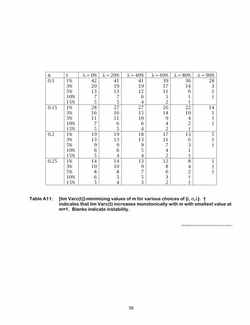
m*. Result V-4 states that increasing λ causes lim Varf(t) to increase. Result V-5 states that increasing λ initially causes lim Varc(t) to decrease but eventually increasing λ beyond λ* causes lim Varc(t) to increase. Hence, it is inefficient to smooth asset values using λ > λ* as there is some other choice of λ for which both lim Var f(t) and lime Varc(t) may be reduced. By symmetry, the second part of Result V-6 also follows. The second part of Result V-6 encompasses the conclusions of Dufresne (1988) who investigates the choice of m when pure market values are used (λ=0). Numerical work indicates that a plot of lim Varc(t) against λ or K has at most one minimum. For any given gain/loss spreading period m, it is inefficient to smooth asset values by more than the [lim Varc(t)]-minimizing value of λ as a lower λ will reduce both lim Varf(t) and lim Varc(t). If m is long enough and lim Varc(t) is strictly increasing with λ, then pure market values should be used. Table A10 lists the [lim Varc(t)]- minimizing values of λ for various choices of {i, σ, m}. It is efficient to smooth asset values using a value λ between 0 and the [lim Varc(t)]-minimizing value in Table A10. By symmetry, Table A11 shows the longest periods over which gains and losses can be efficiently spread for various choices of {i, σ, m}. Thus, the variance of the funding process exhibits dependence on the asset valuation and gain/loss adjustment techniques. They have a complementary smoothing function and consideration should be given to their combined effect. It is apparent that excessive smoothing through very long amortization and averaging periods leads to instability in the pension funding system, which is reasonable because gains and losses are not removed fast enough and they accumulate. Indeed, the funding level becomes more volatile if more

26

smoothing is applied. Contribution rates do become more stable as longer averaging periods are used or as gains/losses are amortized over longer periods, but too much smoothing leads to contribution rates becoming more volatile and is therefore inefficient. If funding is stable, whether exponential or arithmetic smoothing asset valuation methods are use, it is possible to show that the actuarial asset values do not diverge from, and are less variable than, the market value of assets. The actuarial asset values remain realistically close to market values, but exhibit less volatility. (Result V-3). 3.5 Concluding Comments The results indicate that, if exponential smoothing is used, such as when asset values are being written-up with adjustment, and gains and losses are being spread indirectly rather than amortized, then a combination of a spreading period of up to 5 years and a weighting in excess of 20% on current market value is efficient (Owadally and Haberman 2000b). Further numerical work appears to indicate that typical arithmetic averaging periods of up to 5 years (along with gain/loss amortization periods of up to 5 years) appear to be efficient in terms of stabilizing both the funded ratio and contribution rates in pension plans, which lends support to current actuarial practice (Owadally and Haberman, 2000c). Mathematical modelling requires many simplifying assumptions but is useful in analyzing valuation methods and in understanding the intricate relationship between actuarial cost methods, gain/loss adjustment and asset valuation. More research, using numerical simulations and realistic models, is required to compare the various asset valuation methods and to investigate the effect of practical factors such as the IRS 20% corridor rule and the choice of averaging periods. Scenario and stochastic modelling are necessary, as in the use of historical rates of return and economic time series asset models. Further research on this subject is important so that actuaries are better able to address their clients’ needs. With published objective research, actuaries can justify their methods and techniques to other professionals and can consequently represent their clients better and influence the standards set by accountants, regulators and lawmakers. REFERENCES ANDERSON A W. 1992. Pension Mathematics for Actuaries, 2nd ed. Actex Publications, Winsted, Connecticut. BÉDARD D. 1999. “Stochastic Pension Funding in Proportional Control and Bilinear Process”. ASTIN Bulletin 29: 271-293. BELLHOUSE D R and PANJER H H 1981. “Stochastic Modelling of Interest Rates with Applications to Life Contingencies – Part II,” Journal of Risk and Insurance 48: 628-637. BERTSEKAS D P 1976. Dynamic Programming and Stochastic Control. New York: Academic Press. BLACK F and JONES R. 1988. “Simplifying Portfolio Insurance for Corporate Pension Plans”. Journal of Portfolio Management 14(4): 33-37.

27

BOULIER J F, TRUSSANT E and FLORENS D 1995. “A Dynamic Model for Pension Funds Management”. Proceedings of the 5th AFIR International Collquium, Leuven Belgium 1: 361-384. BOWERS N L, HICKMAN J C and NESBITT C J 1979. “The Dynamics of Pension Funding: Contribution Theory”. Transactions of the Society of Actuaries 31: 93-122. CAIRNS A J G 1997. “A Comparison of Optimal and Dynamic Control Strategies for Continuous-time Pension Fund Models”. Proceedings of the 7th AFIR International Colloquium, Cairns, Australia 1: 309-326. Committee on Retirement Systems Research. 1998. Survey of Asset Valuation Methods for Defined Benefit Pension Plans. Society of Actuaries, Schaumburg, Illinois. DAY J G and MCKELVEY K M. 1964. The Treatment of Assets in the Actuarial Valuation of a Pension Fund. Journal of the Institute of Actuaries, 90, 104-147. DHAENE J 1989. Stochastic Interest Rates and Autoregressive Integrated Moving Average Processes”,. ASTIN Bulletin 19 131-138. DUFRESNE D 1988. “Moments of Pension Contributions and Fund Levels when Rates of Return are Random”. Journal of the Institute of Actuaries 115: 535-544. DUFRESNE D 1989. “Stability of Pension Systems when Rates of Return are Random”. Insurance: Mathematics and Economics 8: 71-76. DUFRESNE D. 1994. Mathematiques des Caisses de Retraite. Montreal, Canada: Editions Supremum. DYSON A C L and EXLEY C J. 1995. Pension Fund Asset Valuation and Investment. British Actuarial Journal. 1, 471-557. EXLEY C J, MEHTA S J B and SMITH A D. 1997. “The Financial theory of Defined Benefit Pension Schemes”. British Actuarial Journal 3: 835-966. EZRA D D. 1979. Understanding Pension Fund Finance and Investment. Pagurian Press, Toronto, Canada. FREES E W. 1990. “Stochastic Life Contingencies with Solvency Considerations”. Transactions of the Society of Actuaries 42: 91-148. FAMA E F and FRENCH K R 1988. “Dividend Yields and Expected Stock Returns”. Journal of Financial Economics 22: 3-25. GERRARD R J and HABERMAN S. 1996. Stability of Pension Systems when Gains/Losses are Amortized and Rates of Return are Autoregressive. Insurance: Mathematics and Economics 18: 59-71.

28

HABERMAN S. 1992. Pension Funding with Time Delays: A Stochastic Approach. Insurance: Mathematics and Economics 11: 179-189. HABERMAN S. 1993a. Pension Funding: the Effect of Changing the Frequency of Valuations. Insurance: Mathematics and Economics 13: 263-270. HABERMAN S. 1993b. Pension Funding with Time Delays and Autoregressive Rates of Investment Return. Insurance: Mathematics and Economics 13: 45-56 HABERMAN S 1994. “Autoregressive Rates of Return and the Variability of Pension Contributions and Fund Levels for a Defined Benefit Pension Scheme”. Insurance: Mathematics and Economics 14: 219-240. HABERMAN S. 1997. Stochastic Investment Returns and Contribution Rate Risk in a Defined Benefit Pension Scheme. Insurance: Mathematics and Economics 19: 127-139. HABERMAN S and SMITH D 1997. “Stochastic Investment Modelling and Pension Funding: a Simulation Based Analysis”. Actuarial Research Paper No 102. Department of Actuarial Science and Statistics, The City University, London, England. HABERMAN S and SUNG J-H 1994. “Dynamic Approaches to Pension Funding”. Insurance: Mathematics and Economics 15: 151-162. HABERMAN S and WONG L Y P. 1997. “Moving Average Rates of Return and the Variability of Pension Contributions and Fund Levels for a Defined Benefit Scheme”. Insurance: Mathematics and Economics 20: 115-135. HABERMAN S, GERRARD R J and VELMACHOS D. 2000. “Life Contingencies with Stochastic Discounting using Moving Average Models. Journal of Actuarial Practice 8: 177-210. JACKSON P H and HAMILTON J A. 1968. The Valuation of Pension Fund Assets. Transactions of the Society of Actuaries. 20, 386-436. KINGSLAND L. 1982. Projecting the Financial Condition of a Pension Plan using Simulation Analysis. Journal of Finance. 37, 577-548. MCGILL D M, BROWN K N, HALEY J J and SCHIEBER S J. 1996. Fundamentals of Private Pensions, 7th ed. Philadelphia, Pennsylvania: University of Pennsylvania Press. O’BRIEN T. 1987. “A Two-Parameter Family of Pension Contribution Functions and Stochastic Optimization”. Insurance: Mathematics and Economics 6: 129-134. OWADALLY M I and HABERMAN S. 1999. “Pension Fund Dynamics and Gains/Losses Due to Random Rates of Investment Return”. North American Actuarial Journal 3 (3): 105-117. OWADALLY M I and HABERMAN S. 2000a. “Efficient Amortization of Actuarial Gains/Losses and Optimal Funding in Pension Plans”. Under review. OWADALLY M I and HABERMAN S. 2000b. “Asset Valuation and the Dynamics of Pension Funding with Random Investment Returns”. Under review.

29

OWADALLY M I and HABERMAN S. 2000c. “Asset Valuation and Amortization of Asset Gains and Losses in Defined Benefit Pension Plans”. Under review. PANJER H H and BELLHOUSE D R. 1980. “Stochastic Modelling of Interest Rates with Applications to Life Contingencies”. Journal of Risk and Insurance 47: 91-110. POLLARD J H . 1971. On Fluctuating Interest Rates”. Bulletin de l’Association Royale des Actuaries Belges 66: 68-97. THORNTON P N and WILSON A F 1992. “A Realistic Approach to Pension Funding”. Journal of the Institute of Actuaries 119: 229-312. TROWBRIDGE C L. 1952. “Fundamentals of Pension Funding”. Transactions of the Society of Actuaries 4: 17-43. TROWBRIDGE C L and FARR C E. 1976. The Theory of Practice of Pension Funding. Homewood, Illinois: Richard D Irwin. VANDERHOOF I T. 1973. “Choice and Justification of an Interest Rate”. Transactions of the Society of Actuaries 25: 417-458. WILKIE A D. 1995. “More on a Stochastic Asset Model for Actuarial Use”. British Actuarial Journal 1: 777-964. WINKLEVOSS H E. 1993. Pension Mathematics with Numerical Illustrations, 2nd ed. University of Pennsylvania Press, Philadelphia, Pennsylvania.

30

APPENDIX A Tables A1 – A9: from Owadally and Haberman (2000a) Tables A10 – A11: from Owadally and Haberman (2000b)

Standard Deviation m Funding Level Contribution Rate Spreading Amortization Spreading Amortization

1 19.1% 19.1% 95.26% 95.26% 3 26.5% 24.3% 46.31% 58.31% 5 34.5% 29.6% 37.95% 47.98%

10m*s ≈ 54.6% 42.0% 33.65% 39.56%

15m*a ≈ 79.4% 54.0% 36.43% 37.78%

20 122.9% 67.2% 46.56% 38.50% 25 232.8% 82.2% 78.74% 40.93%

Table A1: Independent and identically distributed rates of return, ϕ = φ = 0.

Standard Deviation m Funding Level Contribution Rate Spreading Amortization Spreading Amortization

1 19.1% 19.1% 95.26% 95.26% 3 34.6% 30.5% 61.24% 75.83%

5m*s ≈ 51.0% 41.2% 54.77% 67.08%

7m*a ≈ 69.3% 52.0% 56.57% 61.24%

10 109.5% 64.8% 67.08% 63.25% 15 273.9% 96.4% 122.47% 70.71% 20 ‡ 148.3% ‡ 89.44% 25 ‡ 214.5% ‡ 111.80%

Table A2: AR(1) logarithmic rates of return ϕ = +0.3. ‡indicates divergence.

31

Standard Deviation

m Funding Level Contribution Rate Spreading Amortization Spreading Amortization

1 19.1% 19.1% 95.26% 95.26% 2 31.3% 27.4% 80.64% 90.83%

3m*s ≈ 43.6% 34.6% 77.46% 88.03%

4 57.4% 44.7% 79.06% 86.60%

5m*a ≈ 74.2% 52.9% 82.16% 85.15%

6 97.5% 61.6% 90.83% 86.60% 7 122.5% 70.7% 104.88% 88.03% 8 167.3% 81.9% 122.47% 94.87%

Table A3: AR(1) logarithmic rates of return, ϕ = +0.5.

Standard Deviation m Funding Level Contribution Rate Spreading Amortization Spreading Amortization

1 19.1% 19.1% 95.26% 95.26% 3 24.5% 23.5% 43.01% 54.77% 5 30.7% 27.6% 33.91% 43.87%

10m*s ≈ 44.7% 37.4% 27.84% 34.28%

15 54.8% 44.7% 28.28% 31.62%

20m*a ≈ 80.6% 53.9% 30.82% 31.22%

25 104.9% 63.2% 34.64% 32.02% 30 130.4% 72.1% 40.62% 33.17%

Table A4: AR(1) logarithmic rates of return, ϕ = -0.1

32

Standard Deviation m Funding Level Contribution Rate Spreading Amortization Spreading Amortization

1 19.1% 19.1% 95.26% 95.26% 2 21.0% 20.5% 36.74% 47.43% 5 24.9% 23.0% 27.39% 36.06% 7 28.5% 25.9% 23.45% 30.41%

10 33.2% 29.3% 20.62% 26.93% 15 40.0% 34.6% 18.71% 23.98% 20 46.9% 38.7% 18.03% 21.79% 25 52.0% 43.6% 18.01% 21.79%

Table A5: AR(1) logarithmic rates of return, ϕ =-0.3

Standard Deviation m Funding Level Contribution Rate Spreading Amortization Spreading Amortization

1 19.1% 19.1% 95.26% 95.26% 3 24.3% 23.5% 42.44% 54.77% 5 30.6% 27.7% 33.62% 43.59%

10 45.1% 35.7% 27.82% 33.91%

15m*s ≈ 60.1% 44.6% 27.55% 31.22%

20m*a ≈ 77.7% 52.0% 26.69% 30.41%

25 102.2% 61.6% 34.51% 31.62% 30 148.1% 71.4% 45.88% 32.40%

Table A6: MA(1) logarithmic rates of return, φ= +0.1.

33

Standard Deviation m Funding Level Contribution Rate Spreading Amortization Spreading Amortization

1 19.1% 19.1% 95.26% 95.26% 2 20.1% 20.2% 35.21% 46.64% 5 23.5% 22.6% 25.82% 34.28%

10 30.5% 27.2% 18.80% 24.49% 15 35.7% 31.2% 16.39% 21.79% 20 39.5% 35.0% 15.10% 19.36% 25 42.0% 38.6% 14.18% 19.10%

Table A7: MA(1) logarithmic rates of return, φ = +0.3

Standard Deviation m Funding Level Contribution Rate Spreading Amortization Spreading Amortization

1 19.1% 19.1% 95.26% 95.26% 3 32.5% 29.7% 56.87% 72.46% 6 45.9% 38.7% 50.47% 61.24%

7m*s ≈ 60.8% 46.9% 50.00% 57.01%

10m*a ≈ 90.1% 56.6% 55.59% 54.77%

12 119.7% 65.6% 64.32% 54.77% 15 209.8% 80.6% 96.18% 57.01%

Table A8: MA(1) logarithmic rates of return, φ = - 0.3.

34

Standard Deviation m Funding Level Contribution Rate Spreading Amortization Spreading Amortization

1 19.1% 19.1% 95.26% 95.26% 3 35.2% 31.6% 61.62% 79.06%

5m*s ≈ 51.5% 41.2% 56.57% 67.08%

7 70.8% 52.0% 58.27% 63.25%

9m*a ≈ 96.9% 60.0% 64.92% 63.22%

10 114.6% 64.8% 70.65% 63.25% 13 219.7% 82.5% 111.39% 65.19% 15 766.2% 94.9% 351.43% 67.08%

Table A9: MA(1) logarithmic rates of return, φ = -0.5.

35

σ i m=1 3 5 10 15 20 25 30 40 50 0.1 1%

3% 5% 10% 15%

97.193.489.982.075.0

96.9 92.6 87.9 73.0 50.4

96.791.483.835.0

4.0

96.0 90.6 22.8

† †

94.8 23.9

† † †

91.6 † † † †

73.1 † † † †

34.5 † † †

32 † †

† † †

0.15 1% 3% 5% 10% 15%

95.992.388.981.174.3

95.5 91.0 86.0 70.2 46.8

94.788.879.328.0

1.1

92.6 55.4 11.1

† †

83.7 5.7

† † †

37.9 † † † †

10.1 † † †

† † †

† †

†

0.2 1% 3% 5% 10% 15%

94.390.887.580.073.4

93.4 88.6 83.2 66.0 42.0

92.084.270.720.2

†

81.5 25.0

† † †

27.1 † † † †

† † † †

† † †

† †

†

0.25 1% 3% 5% 10% 15%

92.489.085.878.672.2

90.3 85.1 79.2 59.9 36.2

86.875.455.612.0

†

39.2 3.6

† † †

† † † †

† † †

†

Table A10: [lim Varc(t)]-minimizing values of λ(%) for various choices of {i,σ,m}. †

indicates that lim Varc(t) increases monotonically with λ with smallest value at λ = 0. Blanks indicate instability.

36

σ i λ = 0% λ = 20% λ = 40% λ = 60% λ = 80% λ = 90% 0.1 1%

3% 5% 10% 15%

422013

75

41 19 13

7 5

41 19 12

6 4

391711

52

36 14

6 1 †

28 3 1 †

0.15 1% 3% 5% 10% 15%

281611

75

27 16 11

6 5

27 15 10

6 4

2614

942

22 10

4 2 †

14 1 † †

0.2 1% 3% 5% 10% 15%

1913

965

19 13

9 6 4

18 13

9 5 4

1711

742

13 6 3 1 †

5 1 †

0.25 1% 3% 5% 10% 15%

1410

865

14 10

8 5 4

13 9 7 5 3

128632

8 4 2 † †

1 † †

Table A11: [lim Varc(t)]-minimizing values of m for various choices of {i, σ,λ}. † indicates that lim Varc(t) increases monotonically with m with smallest value at m=1. Blanks indicate instability.

{Modelling Defined Benefit Pension Schemes/d:research papers }