Modelling and identification of nonlinear dynamic loads …mickgg/docs/Karlsson+Hill.pdf · MODELUNG AND IDENTIFICATION OF NONLINEAR DYNAMIC LOADS IN POWER SYSTEMS ... stability analysis

IEEE Transactions on Power System, Vol. 9, No. 1, February 1994 157

MODELUNG AND IDENTIFICATION OF NONLINEAR DYNAMIC LOADS IN POWER SYSTEMS

Danlel Karlsson Sydtraft AB, S-20509

Malmb, Sweden Abdract This paper describes an approach for experlmental determlna- tionof aggregatedynamlcloadslnpowersystems.Theworkismo- tlvated by the Importance of accurate load modelllng In voltage stability analysis. The models can be expressed In general as nonlinear dlfferential equations or eqihalentty realised In block dla- gram form as lnterconnectlons of nonlinear (memoryless) functions and Pnear dynamic blocks. These components are parameterised by load Indexes and time constants. Experlmental results from tests in Southern Sweden on the ldentlflcatlon of these parameters are described. K.ywords Load modefllng, power systems. dynamlcs. voltage stablllty. 1 InhoducWon Models for dynamlcal analyds of power systems typically have a conslstency problem. while lt issclentlflcally posjible to glve quite detaliedmodels for generators, Ines,transformers and control devices. load modelling can often only be treated on an ad hoc ba- ds. In stabllltyanalysis for Instance. we need a representation of effectlve power demand at high voltage buses. Thls may Include the aggregate effect of numerous load devices such as lighting. heating and motors plus some levels of transformer tap-changing and other control devices. Buildlng up the aggregate effect by combining device characterlstlcs may not be possible. In many cases, quite slmpllfled aggregate load representations like lm- pedances are used alongside detalled generator models. This seems related to three research questions: 1 . To what extent are accurate load models Important In

power system stability analysis; 2. Given that derivation of aggregate models from compo-

nent characteristics is not feasible. what are appropriate mathematical structures to represent high voltage effec- We load;

3. How can the aggregate load models (from question 2) be determined in practice.

Briefly. we refer to these questions as model justification. structure determination and ldentiflcation respectlvely. The present paper Is primarily concerned with model structure and ldentiflcation from SVJtem tests. The study of bad model justification In dynamlcal anaws of power systems seems to demand more attention.The usual aggregate load model expresses the real and reactive load powers as nonlin-

ear functlons of voltage; for instance, the form P O ( 6 ) ‘ wlth a

dngle Index a, for real load power Is popular (with a similar form for reactive power) [ 1-31. Frequency dependence can be Included. but is usually Ignored. For translent (angle) stablllty, there Is stlll some debate about whether acceptable nrst swing assessment can be donewlth lmpedanceload models.i.e. a = 2 ratherthan speclflcally determlned values [4d]. The present work Is motivated more by vdtage stablllty analyds [a. Here It Is widely ac- ceptedthatload characterlstlcs at lowvottage play an Important role; further,dynamlcs of loadsls Important [7.8]. However, the dynamlcal descrlptlon of loads at HV buses certainly requlred more attention. For static (load flow) voltage stability analyds. It Is often assumed that the load powers are In fact constant, I.e. a = 0. In

93 WM 171-9 PWRS by the IEEE Power System Engineering Committee of the IEEE Power Engineering Society for presentation at the IEEE/PES 1993 Winter Neeting. Columbus, OH, January 31 - February 5, 1993. Manuscript submitted August 25, 1992; made available €or printing December 3. 1992.

A paper recommended and approved

David J. Hill, Senlor Member The Unhrerslty of Newcastie.

Callaghan, NSW 2308, Australla order to reflect voltage control adon by tapchangers and switched capacitance. This is not approprlate In me study of dynamlc behaviour. This paper Is an outcome of projects In Sweden alming to develop dynamlcal load models and study voltage dynamlcs followlng large dlsturbances. A study of dynamlcd load modelflng waslnltl- ated by Karlsson and Pehrsson [9]. Walve [8] commented on their model while discussing the Importance of load modellng In urt derstandlng the 1983 Swedish blackout. The model In [O] Included a dynamlc voltage term wtthin a linear structure. Observations of field load transient responses led Edstdm and Wake [ 101 to study In more detall some nonlinear aspects of load recovery followlng a voltage step. Although voltage collapse In general is a phenom- enonthattakesseveral mlnutes,ltwclsrecognlzedthotmostofthe load modelling work so far had concentrated on hductlon machines in the range of seconds after a disturbance. The alm wcls to develop accurate load models for voltage stabilly studies, Val- Id for at least several minutes after a disturbance. However, at this staae no (nonlinear) model relating general voltage to power slg- nals was proposed. Hill [ 1 1 1 proposed such a model wlth a simple nonllnear structure deflned by two nonlinear fu~ctlons and a r e - covery time constant. Thls was subsequently usBC1 to explore static vs dynamic aspects of voltage stablllty [ 12-14]. Meanwhlie Kark son et. al. devisedexperiments to record load responsestovarlow voltage signals [ 151. This data ms used to identify a particular recovery model which can be derived from the general Input-output dynamlcal model described earller In [ 1 1 , 12].The load functions were assumed to have the single Index form. Thls paper alms to present a coordlnated discussion of the overall load modelling approach covering model structures and parameter identiflca- tion. The dlscusslon of structures blends Ideas presented prevlcusly by Hlll [ 1 1. 131 and Karlsson [ 151; results from the recent thesis by Karlsson [ 161 are wed to illustrate model parameter ldentiflcation from fleld tests. The structure of the paper Is as follows. Section 2 discusses typical load responses and their representation as solutions of nonllnear differential equations. These can be expressed in hlgher-order scalar or flrst-order vector form. It Is also convenient to view the models as block diagram interconnections of nonlinear functions and llnear dynamic blocks. Section 3 revlews technlques for parameter ldentiflcatlon in nonlinear systems. %don 4 follows Chapter 3 of the the& [ 161 to Illustrate recovery model ldentiflcation from fleld tests; a one dlmenslonal model with dngle Index steady-state and translent load functlons Is Identifled for data re- flecting seasonal varlatlon. 2 General load Model struchrres Consider a high voltage bus as In Rgue 2.1. The real and reactlve power demands Pdand Qd are considered to be dynamlcally related to the voltage v

Figure 2.1 High Voltage Load Bus

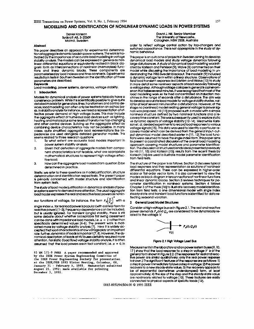
Measurementslnthelaboratoryandonpowersystem buses[O. 10, 171 show that the load response to a step in Wage Y Is of the general form show In Rgure 2.2. (The responses for real andreac- tive power are dmiar qualltalivdy; only me red power response Is show.) The slgnlflcant features of the response are as follows: 1) a stepin powerlmmedlatelyfollowsasteplnvdtage;2)thepower recovers to a new steady-state value; 3) the recovery appears to be of exponential (sometimes underdomped) form. at least approxlmately; 4) the size of the step and the steady-state value are nonlinearly related to voltage [lo]. These features ate eadly connected to physlcal aspects of specltlc loads 1131. - -

0885-8950/94/$04.00 Q 1993 IEEE

158

v vo- v,.

p,

PI

I Fgure 2.2 Gened Load Response

As in [ 131, we can propose a general load model as an lmpllcl dit- ferentia1 equatlon

f(p’c!p’;-’’ ,..., i,,P,V+), *-1) ,... 3.v) * 0 (1)

where Pif . tivdy. (A similar e q u w n applies for reactive power e,,) For llrst order dynamics, equatlon (1) becomes

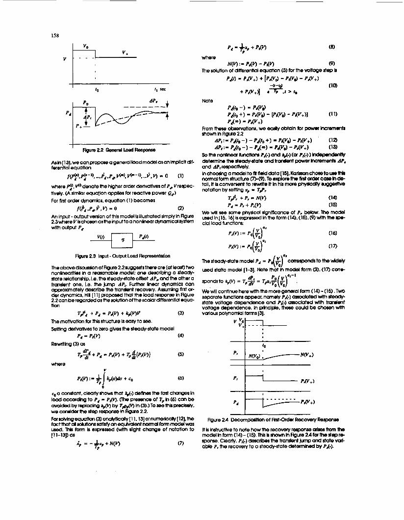
An Input - output version of this model Is Illustrated simply In Rgure 2.3whereV Ischosenasthelnputtoa nonlinear dynamicalsystem

denote the hlgher order derivatives of P,,, Vrewec-

f(P,,P,kv) = 0 (2)

with output P+

- - - - I

I

I

10 I

NWO) If W+)

I

I PXV,)

Feure 2.3 Input - Output Load Representation

The above discussion of Figure 2.2 suggeststhere are (at least) WO nonPneaMes in a reasonable model: one describing a steady- state relationship. I.e. the steady-state offset AP, and the other a translent one, i.e. the jump AP,. Further linear dynamics can approxlmatety describe me translent recovery. Assuming first order dynamlcs. HI1 [ 1 11 proposed that the load response in Figure 2.2can beregardedasthe sokrtlonofthescalar differentrd equa- non

The mottvation tor this structue Is easy to see. Semng derlvatlves to zero gives the steady-state model

Rewrttlng (3) as

T#, + Pr = pxv) + J!p(Y)y

p , = pxv) (4)

(3)

where

Pm : = 1 kp(0)da + CO (6) TP [

c0 a constant, clearly shows that k,(-) defines me fast changes In load according to P, = P,O. presence of T, In (6) can be avoided by replacing k,o by 7&,0 In (31.1 To see this preclse)Y. we conalder the step response in Rgure 2.2. FortoMng eqwtlon (3) analytically [ 1 1.131 or numerically [ 12],the fact that al wlutlons satisfy an equhrdent normal form model was used. This form Is expressed (with slight change of notatlon to [ 1 l-np as

;e = -Lp +N(v) m TP

(16)

(17)

The steady-state model P,

used stalk model [ 1-31, Note mat In model form (3). (17) cone

I ~~~

Figure 2.4 Decompbdtion of RntOder Recovery ReSpoMe

It is instructive to note how me recovery response arloer frun the model in form (14) - (15). This is shown In Figure 2.4 forthe step response. Clearly. PA.) describes the transient Nmp and state vari- able P, the recovery to a steady-state determined bv PA.).

159

N2(*)

V

r

PI

I I . (a)

(b)

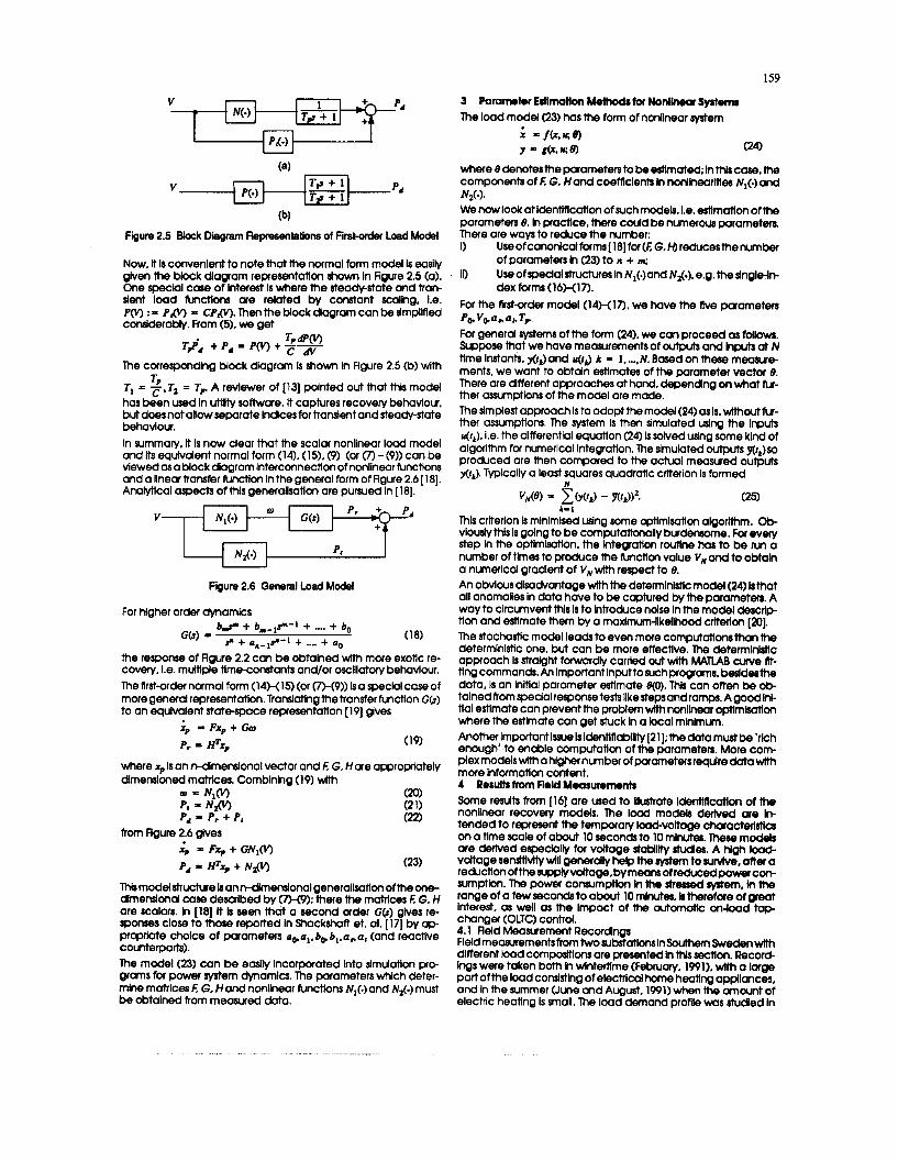
Figwe 2.5 Block Diagram Representahns of First-arder Load Model

Now, It Is cormenlent to note that the normal form model Is easily given the block diagram representation shown In Flgure 2.5 (a). One speclal case of Interest Is where the steawstate and translent load hctlons are related by constant scaling, I.e. P o : = P,O = CPXV). Then the block diagram can be dmpllfied conslderably. From (5). we get

The corresponding block diagram is shown In Agure 2.5 (b) with

T, = F, T~ = T,,. A reviewer of [l3] polnted out that this model has been used In utility software. it captures recovery behaviour, but does not allow separate Indices for translent and steady-state behaviour. In summary, tt Is now clear that the scalar nonlinear load model and Its equlvalent normal form (14). (15). (9) (or (7) - (9)) can be viewed as a block diagram Interconnection of nonlinear functions and a llnear transfer function in the general form of Agure 2.6 [ la]. Anaiytlcal aspects of this generalisation are pursued In [la].

T P

For higher order dynamlcs

the response of Figure 2.2 can be obtained with more exotic recovery. 1.8. multiple tlme-constants and/or osclilatory behaviour. The first-order normal form (14>-(15) (or (7)-(9)) Is a speclal case of more general representation. Translatlngthe transfer function C(S) to an equivalent state-space representation [ 191 gives

xp = Fxp + Go

P, 5 HTxp (19)

where xp Is an Mmensional vector and E G, Hare approprlately dlmensloned matrlces. Combining (19) wlth

@J = 403 (20) PI = N*03 (21) P, = P, + P, (22)

from Figure 2.6 glves Xp F x ~ + G N 1 o P, - HTxp + N m (23)

Thb model atructue is an n-dlmenslonal genefallsation of the one- dlmenslond case descrlbed by (7x9); there the matrlces E G. H are scalars. In [18] It ls seen that a second order G(s) gives responses close to those reported in Shackshaft et. al. [ 171 by approprlate choke of parameters uoal.bb bi.a,uI (and reactive counterparts). The model (23) can be easily Incorporated Into slmulation programs for power system dynamlcs. The parameters whlch deter- mine matrlces E G. Hand nonlhear functions NJ.) and A$(.) must be obtained from measwed data.

. , . .. . . .~

3 Parameter EdimaWon Methods for Nonlinear Systems The load model (23) has the form of noninear system

x =fcr.se) Y - rCr.w;e) (24)

where e denotes the parameters to be estimated; In t M s case. the components of E G, Hand coefnclents In nonlheamea Nl(.) and

We now lock at Identlficatlon of such models. I.e. estimation of the parameters 8. in practlce. there could be numerous parameters. There are ways to reduce the number: I) Use of canonical forms [ la] for ( E G. H) reducesthe number

of parameters h (23) to R + ti ID Use of special structures In Nl( . )and N&), e.g. the slngbln-

d e x forms (16x17). For the llrst-order model (14x17). we have the five parameters

For general systems of the form (24). we can proceed as follows. Suppose that we have measurements of outputs and Inputs at N time Instants. r(f3 and 4r3 L = 1. .... N. Based on these measurements, we want to obtain estimates of the parameter vector e. There are different approaches at hand. depending on what further assumptions of the model are made. The simplest approach is to adopt the model (24) as Is, without further assumptions. The system is then simulated using the Inputs 413, I.e. the dlfferentlal equation (24) is solved using some kind of algorlthm for numerical Integration. The simulated cutputs y(tk)so produced are then compared to the actual measwed outputs f i rk) . Typically a least squares quadratic crtterlon Is formed

N2(*)*

Pa. Vbur 01. Tp

N

v,m = XWJ - kdl2 . (25) k-1

This criterion is minlmlsed using some optlmlsatlon algorithm. Ob- vlously thls Is going to be computattonaly burdensome. For every step In the optlmisatlon. the Integratlon routlne has to be run a number of times to produce the function value V,and to obtain a numerlcal gradlent of VN with respect to 8. An obvlous dlsadvantage with the determlnlsnc model (24) kthat all anomalies In data have to be captured by the parameters. A way to circumvent thls is to introduce noise In the model descrlp tlon and estlmate them by a madmum4kellhood crtterlon [XI]. The stochastic model leads to even more computatronsthan the determlnlstlc one. but can be more effectlve. The determlnlstlc approach Is stralght forwardly carrled out with MATLAB curve llt- ting commands. An Important Inputto such programs. besldesttie data, Is an inttial parameter estimate e@). This can often be obtained from special response tests like steps and ramps. A good Id- tlal estimate can prevent the problem with nonlinear optknisatlon where the estimate can get stuck In a local minknun. Another Impcftant Issue lsldentiflabllity[21]:the data must be 'rich enough' to enable computation of the parameters. More complex models Wrth a hlgher number of parameters requlre data wlth more Information content. 4 Results from Field M.asuromenh Some results from [ 161 are used to Ulustrate ldentlficatlon of the nonlinear recovery models. The load models derived are In- tended to represent the temporary load-vottage characterlstics on a time scale of about 10 seconds to 10 mlnutes. These models are derived especially for voltage stability dudes. A hlgh load- voltage SensiIMty wHI generally help the system to survive, after a re&ction ofthesupph/vdtage.bvmeonsof reducedpowercor, mptlon. The power consumption In the stressed system, In the range of a few seconds to about 10 minutes, b therefore of oreat interest, as well as the Impact of the automatic on-load t a p changer (OLTC) control. 4.1 Reld Measurement Recordings Fleld measurements from two substations In Southem Sweden wlth different load compoSmons are presented In thls sectlon. Record- lngs were taken both In wintertime (Febwary, 1991). with a large part of the load conslstlng of electrical home heatlng appllances, and In the summer (June and August, 1 9 9 1 ) wtren the amount of electric heating Is small. The load demand profile was studied In

160

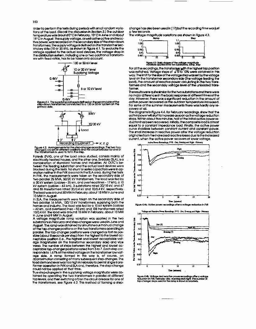
order to perform the tests during periods wlit~ small random varlatlons of the load. (Recdl the dhscussion in Section 3.) The outdoor temperatwewasarmdO'C in February, 1O'C InJune andabout 18'C lnAugust.TheSupph/voltage.aswellastheactiveandreac- tivepower,wasrecordedonthesecondarysldeofthestepdown transformers.fhesupphlv~~ekrdefinedonthetransformersec- ondary side (10 or 20 kv), as shown In Figure 4.1. To evaluate the voltage applled to the actual bad devkes, the voltage drop In the dMributlon system, Including one or two addmonal transformers with fixed ratios. has to be taken into account.

130 or 50 kV level

e

0.

6 or 10 kV level

.' I Recordlng W V R Q quipmen

%m 4.2. Armngemenls for the step-charvg feco@gSs. T h e two tap c clrcutt-breaker fa one of the trorisforrnm is used to form the step.

Fotevik (FVK). one of the load areas studied. consists mainly of electrically heated houses, and me other one, Svedala (SLA). is a combinatlon of standard homes and Industries. All OLTC's between the feeding substation and the actual load devices were blocked durlng the tests. No shunt or series capacitors were In operation neither lnthe FVK area nor inthe S I A area, during me tests. in M, the measurements were taken on the secondary side of two parallel 25 MVA. =/XI kV transformers. The load was fed by a 20 kV system (cables- 35 km, and overhead lines - 17 km), a 10 kV system (cables - 63 km), 3 substations rated 201 10 kV. and 47 and 85 transformers rated 20/0.4 kV and 10/0.4 kV, respectively. The load was around 30 MW in February, about 18 MW in June and 10 Mw in August. In SlA. the measurements were taken on the secondary side of two parallel 16 MVA, 130/10 kV transformers, supplying both the homes and Ind~stty. The load was fed by a 10 kV system (cables - 42 km. and overhead lines - 55 km) and 108 transformers rated 10/0.4 kV. The load w a s around 15 MW in February, about 10 MW in June and 0 MW In August. A voltage magnitude ramp variation was applied in the two substations in February and stepchanges were used in June and August. The ramp was obtained by dmultaneousmanual change of the tapchanger positions on the two transformers operating in parallel. The tagchanger poSmons were changed as fast as possible (about 8 seconds per step) from the highest to the lowed acceptable poJmon 0s.. the hlghest and lowest acceptable voit- age magnitudes on the transformer secondary side) and vice versa. The rumber of steps between the highest and lowest acceptable tapchanger posltim varied from 5 to 7. Each step cor- responds to 1.67% of the rated voltage on the transformer iowvolt- age aide. A ramp formed In this way is, of course, an approxlmotbn consisting of many subsequent step-chonges. The load demand level was too high In February to permit Jingle transformer operation In M( and SLA and,therefore, the step-change could not be -Red at that time. True stepchanges h the supplying voltage magnitude were ob- talned by operating the two transformers In parallel at different tapl8VelS. and then swltchlng off/on the ckcuit-breaker for one of the transformers. see Figwe 4.2. Thls method of forming a step-

ngen are set atdfferent p o s m and

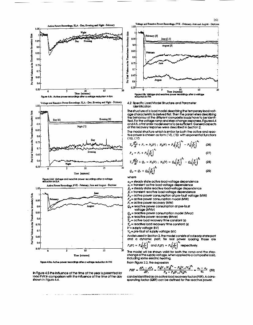
change has also been wed in [ 171 butthe recording time was just a few seconds. me voltage magnitude vcwlalions are shown In Flgure 4.3.

1.1

0.95 0.9

0.85 0.M

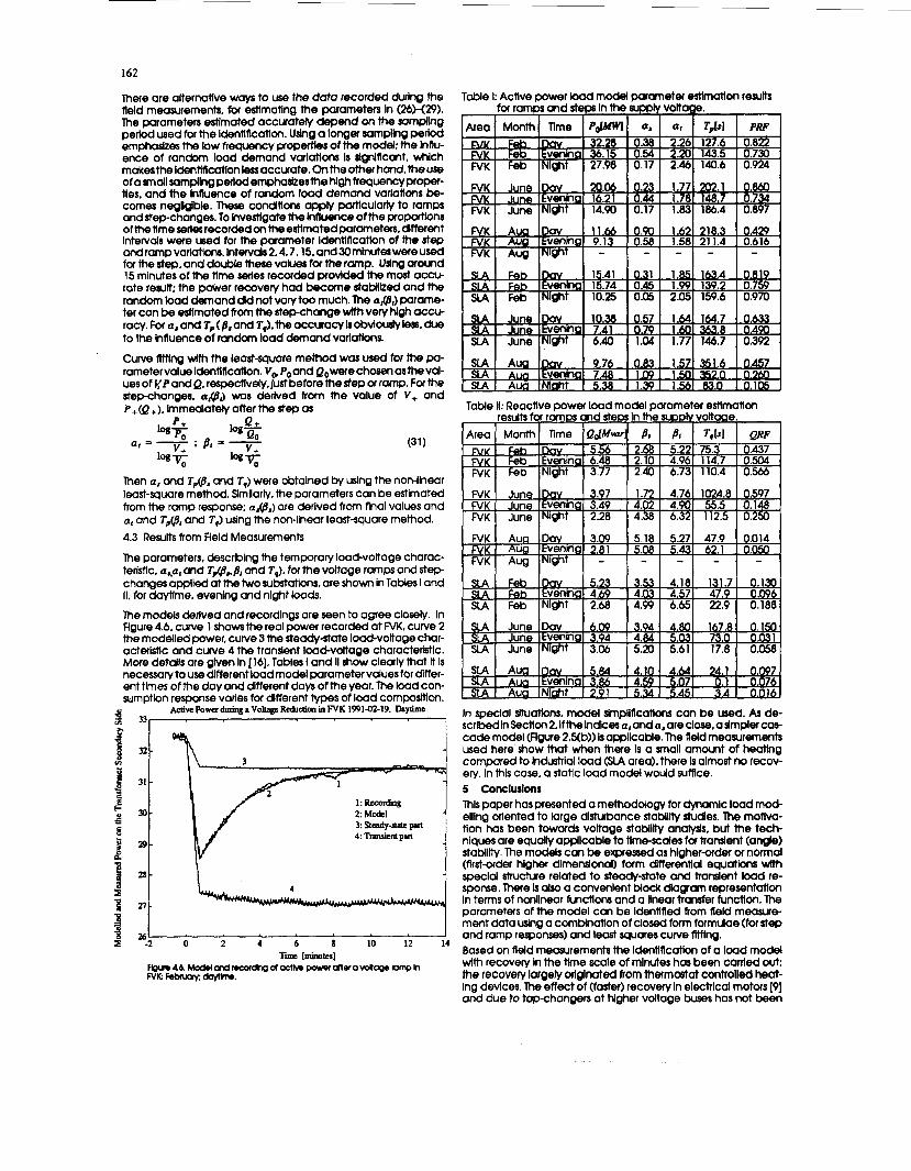
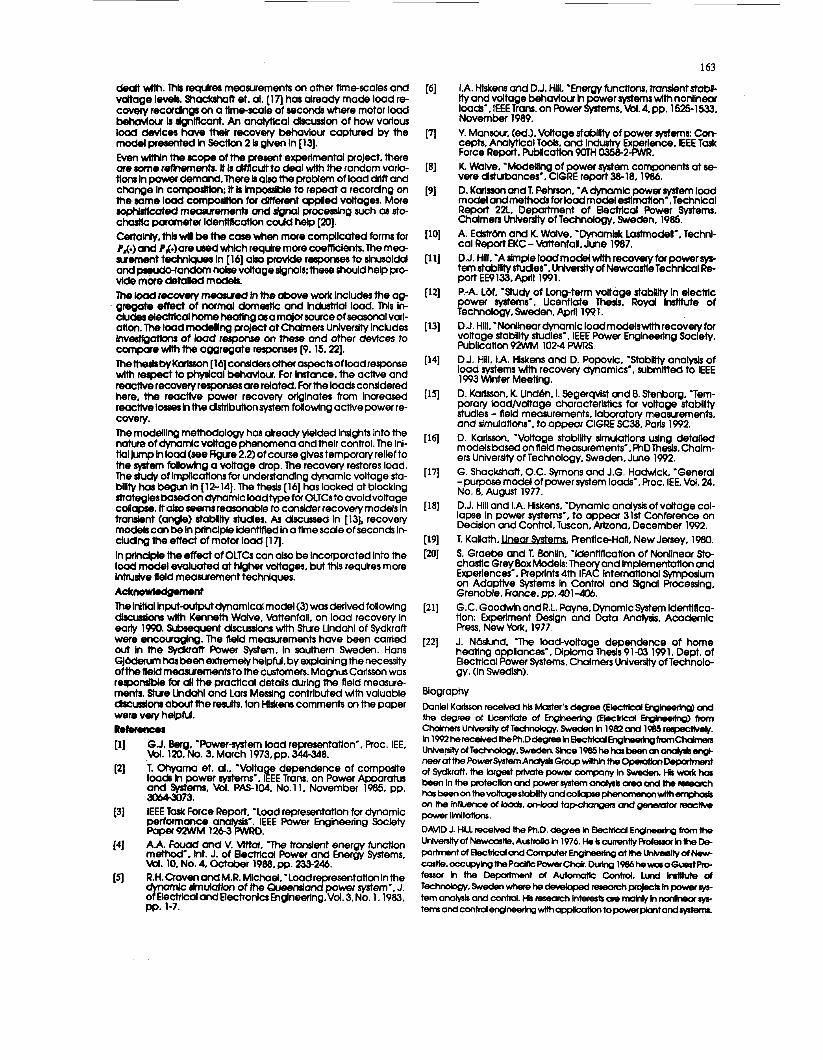
For all the recordings. the transfor g@h me highest top poSmon was witched. Voltage steps of *%! 10% were obtained In this way. The limit forthe &e ofthe voltage step wasset bythevottage level on the transformer secondary dde (me voltage feeding the load). the amount of reactive power clrculaiing In the two transformers and the seconduty voltage level of the unloaded transformer. The results were qulteslmllur forthetwo substations andtherewere no major differences in the basic response d different limes of the day. However, there wos a dgnlflcant reduction In the amount of acthre power recovefed as the outdoor temperoture Increased. For some of the Summer measurements there w a s hardy any recovery at ail. The diagrams In Agure 4-4. for February recordhgs, show that the acthre powerwlistarttolncreaseassocn asthevoltagereduclion stops. Within about tlve minutes. half of the initial active power reduction has been recovered. Inltlally.the composite load balmost equal to a constant Impedance load. Fhally, the actlve power curve stabiikes between constant current and constant power. The small Increase In reactive power after the voltage reduction orlglnates from the Increased reactive losses due to the increased current, when the actlve power recovers at lower voltage.

1.05, . 1 MiwRolcraosolQpFn-rE=bI=ldNii-kblwy

0.9

0.85

161

1.05

8 1 i 0.95

+ 09 1 0.85

B 0.8 b

0.75

' 0.7 0

? .z 0.65 9 2 0.6

0.55 0 5 10 I5 m Time [mimtal Fb~n45b. Wboe ond nocNvr POWCH mcofdw b r a wit-

rPductbnhM( Fbun4dc. k t k s powrrecordngr dteravmm nductba hSlA

4.2 Speclflc Load Model Structure and Parameter

The structure of a load model describing the temporary load-voltage characterisHc is derived Wst. Then the parameters describing the behaviour of the afferent composite loads have to be ldenti- fled. Forthevoltage ramp andstepchange responses. Rgures4.4

; 0.9 and4.5.aflrstordermodel~eemstobe~ufticient. General aspects of this recovery response were descrlbed In Section 2. The model structure which is slmUar for both the actlve and reac- 2 s 0.8 tlve power is chosen as form (14). (15) with exponentlal functions

+ (16). (17)

1.05 identification d l 5 0.95

! 0.85

0.75 dP at 0 Tp* + P, = N p 0 ; NAV) = P o ( t r - P (L)

P, = Pr + P O ( 6 )

T,T (der + Qr = N , O ; N,O = Q,(t- - Q T i [mirnucsl Qd Qi + Q o ( t ) (29)

(26)

(27)

(28)

f 0.7 vo : 2 0.6

0 1 - .z 0.65 3

O vo 5 10 I5 20 PI

0.55 0

F l O u e 4 P d ~ ~ o n d r e o c t h r e ~ r e c o r d h g r d t e r o ~ ~ e where mductbnhSlA as = steady state active load-voltage dependence

at = transient acme load-voltage dependence ps = steady state reactlve load-Wage dependence pI = transient reactive load-voltage dependence Po = active power Consumption at pre-fault voltage (MW) Pd = active power consumption model (Mw) P, = active power recovery Q, = reactbe power consumptlon at pre-fault

Q, = reactlve power consumption model (Mvar) Qr = reactive power recovery [Mvar) T,, = actlve load recovery time constant ts) r, = reactive load recovery t h e constant (si Y = supply voltage (kv) V, = prsfault of supply voltage 0 As d k w d In Section 2,the model cwlsts of a steady-state part and a dynamlc part; for real power loading those are

Pxv) = P o ( t ) and P,O = P , ( e ) respectively.

0 5 10 1s The model will be shown valid for both the ramp and the s t e p change of the supply vottage. when applled to a composite load, includng some electric heating. From Hgure 2.2. the expression

1.05

4 1

1 0.9

1 0.85

1 0.75 s 4 0.7 5 0.65

8 0.95

voltage [MVcirl c

1 0.8 +

2 0.6 as 8 1

0.55

TW [-le81

Figu04.S~ Acth paunmuxdhgs dhtavolta&p mcbcllon hM<

AP, - AP, PdV+/Vo)'' - po(v+/vo)a' a1 - a, at (30)

can be identified as an actrveload recovery factor (PRO. A cwe- spondlng factor (QRF) can be deflned for the reactive power.

PRF=-= In Agure 4,5 the influence of the llme of the year Is presented for API Po - PO(Y+/vd"l load N K In comparison wlth the Influence of the tlme of the day shown in Rgure 4A.

162

mere are alternath/e wys to use the data recorded durlng the field measurements, for estimating me parameters in (26x29). The parameters estimated accurately depend on the sampllng period used for the Identification. Uslng a longer sampling period emphasizes me low frequency properties of the model: the hfiu- ence of random load demand varlations Is significant. whlch makes the identification less accwate. On the other hand, the USB of a smdl sampllng period emphashesthe high frequency properties, and the influence of random load demand varlatlons becomes negligible. These condltions apply particularly to ramps and step-changes. To hvestlgate the In(krence of the pfopoftlons of metlme series recorded on me estimated parameters, different Intervals were used for the parameter ldentlfication of me step and ramp varlatlons. Intervals 2,4,7,15, and 30 minute8 were used for the step, and double these values for the ramp. Uslng around 15 minutes of the time series recorded provided the most accurate result: the power recovery had become staMibed and the random load demand did not vary too much. The U#,) parameter can be estlmated liom the stepchange wlth very hlgh accu- racy. For a,and ~,(p.and T,).theaccuracyIsobvlouslyler.due to the hlluence of random load demand variatlons.

Curve lltling wlth the least-square method was used for the pa- rametervalue identification. V, P,and Q,werechosenasthevai- ues of yP and Q, respectively. Just before me step 01 ramp. For the step-changes. a&) was derived from the value of V+ and P+@ +). knmedlately after the step as

32.28 0.38 2.26 127.6

‘ NK F e b Nlght 27.98 0.17 2.46 140.6 lnz~ 36.15 0.54 2.20 143.5

Then a, and Tp(8. and T,) were obtained by uslng the non-linear least-square memod. Similarly, me parameters can be estimated from the ramp response: a,@.) are derived from final values and (I~ and T#jS, and T,) using the non-linear least-square method. 4.3 Results from Field Measurements

The parameters, describing the temporary load-voltage characteristic. a,a, and T,~..@, and T,), for me voltage ramps and stepchanges applled at the two substations, are shown in Tables I and 11. for daytime. evening and night loads.

The models derived and recordings are seen to agree closely. in Rgure 4.6, curve 1 showsthe real power recorded at N K . curve 2 the modelled power, curve3 the steady-state load-voltage characteristic and curve 4 the transient load-voltage characteriktlc. More details are w e n in [ 161. Tables I and I1 show clearly that lt Is necessary to use different load model parameter values for dlffer- ent tlmes of the day ond different days of the year. The load con-

0.822

0.924 0.730

sumption response varies for different types of load composition. Acci~Po~adrmnpaV~llapeRdlctioninFVK 199142-19. Daytime

20.06 16.21

NK June Maht 14.90

33,

0.23 1.77 202.1 0. 0.44 1.78 148.7 -d&- 0.17 1.83 186.4 0.897

32t “i-a, 3

, N K Aua Dav 11.66 0.90 1.62,218.3 0.429 NK AUG ‘€venlna 9-13 0.58 1.58 211.4 0.616 N K Aug Night - - - - -

Table I: Active power bad model parameter estimation results

[Area I Month1 Time I P d W I 0, I at I T,K4 I PRF

for romps and steps In the supply voltage.

FVK NK FVK

Feb Dav 5.56 2.68 5.22 75.3 0.437 Feb Evening 6.48 2.10 4.96 114.7 0.504 Feb Night 3.77 2.40 6.73 110.4 0.566

FVK FVK FVK

June Dav 3.97 1.72 4.76 1024.8 0.597 June E V W h Q 3.49 4.02 4.90 55.5 0.148 June Nlsht 2.28 4.38 6.32 112.5 0.250

Table 11: Reactive power load model parameter estimation results for ramm and stew In the su~ptv voltasae.

/Area I Month] Tlme lQOfMwri A I 6, I T,bI I QW I

FVK NK FVK

Aua Dav 3.09 5.18 5.27 47.9 0.014 AUg Evening 2,8i 5.08 5.43 62.1 0,050 Aug Night - - - - -

in special situations, model slmpilficatlons can be used. As de- scribedlnSection2,Iftheindkes a,andu,areclose,asimplercas- cade model (Hgure 2.Xb)) Is appi1cable.The field measurements used here show that when there is a small amount of heating compared to industrial load (SlA area). there Is almost no recovery. In this case. a statlc load model would suffice. 5 Conclurlons This paper has presented a methodology for dynamic load modelling orlented to large disturbance stabUity studies. The motivation has been towards voltage stability analyds. but the tech niques are equally applicable to time-scales for transient (angle) stabillty. The models can be expressed as hlgher-cfder or normal (flrst-order higher dimensional) form differentlal equations wtth specld structure related to steady-state and transient load r e sponse. mere Is also a convenient block diagram representation In terms of nonlinear functions and a #near transfer function. The parameters of the model can be Identified from field measurement data uslng a combbmtion of closed form formulae (for step and ramp responses) and led squares curve fiillng. Based on fleld measurements the ldentificution of a load model with recovery In the time scale of minutes has been carried out; the recovery largely orlglnated from thermostat controlled heating devlces. The effect of (faster) recovery In electrical motors [O] and due to tapchangers at hlgher voltage buses has not been

163

LA. Hiskens and D.J. H111. 'Energy funcflons, transfent stab#- Hy and voltage behaviour In power systems wtth nonllnear loads', IEEE Trans. on Power Systems. Vol. 4. pp, 1525-1533, November 1989. Y. Mansour, (ed.), Voltage stabltlty of power systems: Con- cepts, Analytkal Took. and Industry rience. IEEE Task Force Report, RrMcatlon POM oJ5&%R. K. Waive, 'Modelling of power system components at se- vere disturbances', CIGRE report 38-18.1986. D. Karlsson and T. Pehrson. 'A dynamic power system load modelandmethcdsforloodmodel estimation',TechnlcaI Report 22. Deparhnent of BecMcal Power Systems, Chalmen UnhreMy of Technology. Sweden. 1965. A. Edstrdm and K. Wdve, 'Dynamlsk Lastmodell', Techni- cal Report EKC - Wenfal, June 1987. DJ. Hill, 'A simple load model with recovery for powr tem s t a w studes'. UniveMy of NewcasfieTechnlcal Re- port EE9133.Apfll1991. P.-A. Ldf, 'Study of Long-term voltage staMlHy In electric power systems-. Ucentlate lheds. Royal Insmute of Technology, Sweden. April 1991. D.J. Hill, 'Nonllnear dynamlc loadmodelswlthrecoveryfor voltage stability studles'. IEEE Power Engineering Society, Publication 92WM 102-4 PWRS. D.J. Hill, IA. Hiskens and D. pOpovlc. 'stability analysis of load systems with recovery ctynamlcs'. submitted to IEEE 1993 winter Meeting. D. Karisson, K. Undbn. I. Segerqvist and B. Stenborg. 'Tem- porary loadfioltage charactertstlcs foc voltage stabllity studies - field measurements. laboratory measurements, and simulations', to appear ClGRE SC38. Park 1992. D. Karlsson. 'Voltage stability simulations wing detailed models based on field measurements'. FhDThesis. Chalm- ers University of Technology, Sweden, June 1992. G. Shackshaft, O.C. Mons and J.G. Hadwlck, 'General - purpose model of power system loads'. Roc. IEE. Vol. 24, No. 8. August 1977. D.J. Hill and I.A. Hiskens. 'Dynamlc analysis of voltage collapse In power systems-, to appear 31st Conference on Decision and Control. Tuscon. Arhona. December 1992. 1. Kanath, lhg&&u& RenticeHall. New Jersey, 1980. S. Graebe and 1. Bohfln, 'IdenMcation of Nonllnear So- chastic Grey Box Models: Theory and Implementation and Experiences', Preprints 4th IFAC International Symposium on Adaptive Systems In Control and Signal Rocesslng, Grenoble. France. pp. 401-406. G.C. Goodwin and R.L. Payne. Dynamic System Idennnca- tlon: Experiment Design and Data Analysis, Academic Press. New York, 1977. J. NWund. 'The load-voltage dependence of home heating appliances'. Diploma Thesis 9143 1991, Dept. of Electrlcal Power Systems. Chalmers University of Technolo- gy. (In Swedish).

dedt wilh. lhk requires measurements on other timescales and vottage leveh. Shackshaft et. al. [ 17l has already made load recovery recordngs on a timescale of seconds where motor load behaviour b dgnlflcant. An analytical ditcusdon of how various load devices have their recovery behaviour captured by the model presented h Sectlon 2 is ghren In [13]. Even WmJn the scope of the present experimental project. there are m e retlnements. It b drmcudt to deal with the random variatlons In power demand. lhere Is also the problem of load drift and change In composmOn: it b hpossrble to repeat a recordng on the same load composmon for different applied voltages. More sop"cated meaaxementa and dgnal processing such as sto- chostlc parameter idennnccmn could help [m]. CertaWy, this wil be the case when more complicated forms for PA.) and P,+)are used whlch requlre more coefticlents. The measurement techniques In [ 161 also provide responses to slnwoidd and psudwandom ndse voltage signals; these should help provide more detalled models. me food recwery meor~ed ln the above work lncludes me aggregate effect of normal domestic and Industrial load. Ns ln- ckrctea electrical home heating as a major source of seasonalvarl- don. The load modeling proJect at Chalmers Unlversiiy Includes investlqatkns of load response on these and other devices to compare wtth the aggregate responses p. 15,221. Thethesisby Karlsson [ 161 considers other aspectsof load response Wm respect to physical behavlou. For Instance, the active and reactlve recovety responses are related. Forthe loads considered here, the reacthre power recovery orlglnates from inoreased reactive losses In the dstrlbuiion system fdowlng active power recovery. The modellng methodology has already yielded lnslghts into the nature of dynamic voltage phenomena and their control. The Ini- tia1)ump In load (see Rgue 2.2) of course gives temporary relief to the system fdbwhg a voltage drop. The recovecy restores load. The study of Implications for understanding dynamic voltage sta- blllly has begun in (12-141. The the& [16] has looked at blocking hategiesbasedondynamicloadtypeforOLTCstoavoidvoltage Collapse. It ako seems reasonable to conslder recovery models In translent (angle) stabilHy studes. As discussed in [13], recovery models can be In principle Identified In a time scale of seconds In- cludng the effect of motor load [ 13. In principle the effect of OLTCs can also be Incorporated Into the load model evaluated at higher voltages. but this requires more Intrusive field measurement techniques. Acknowkdg.nwnt The Initial hput-ouiput dynamical model (3) was derlved following dlscu9i00, with Kenneth Waive, Wtenfall, on load recovery in early 1990. Subsequent dlscusslons with Sture Undahl of Sydkraft were encouraglng. The field measurements have been carried out in the Sydkraft Power Wem, In southern Sweden. Hans GJMerum has been extremely helpful. by expiainlng the necessity of the fieM measurements to the customers. Magnw Carlsson was responsible for all the practlcal details during the fleld measurements. Siue Undohi and Lars Messing contributed with valuable dscus5iiorrr about the results. Ian Hiskens comments on the paper were very helpM. R O r e f ~ 8

[l]

(21

G.J. Berg, 'Pow-system load representation', Roc. IEE, W. 120. No. 3. March 1973, pp. 344-348. 1. -ma et. al.. 'Volta e dependence of composite loads In power systems'. f E E Trans. on Power Apparatus and Systems. Vol. PAS-104. No.11. November 1985, pp. 3064-3073. IEEE Task Force Report. 'Load representation for dynamic perfmance anah/sls'. IEEE Power Engineering Society Paper92WM 126-3 M D . AA. fowd and V. Vlttal, 'The transient energy function method'. Int. J. of Electrical Power and Energy Systems, Vol. 10, No. 4. October 1988, pp. 233-246. R.H. Craven and M.R. Michael. 'Load representation In the

mlc dmulatton of the Queensland power system'. J. ~lcalandElectronlcrEnQneerlng.Vol. 3,No. 1.1983,

(31

[4J

[SI

W. 1-7.

164

Discussion

M. K. Pal: As stated in the introduction, the load modeling work reported in the paper was motivated by current work in voltage stability. Our comments, likewise, apply mainly to voltage stability analyses. In vast majority of voltage stability analyses, a higher order dynamic load model is not really necessary. Voltage stability is determined by overall dynamic behavior of the load. The overall response speed of aggregate load is generally slow. Therefore, a first order model should be sufficient. The authors basically seem to agree with this contention. Based on field measurements, they have also identified a first order load model for loads with slow recovery time. The significant features of the aggregate load response as observed by the authors in laboratory and field tests are also what one would expect from the known behavior of the individual load devices and/or from well estab- lished mathematical models of these devices.

A higher order model might be appropriate in a general stability analysis that encompasses voltage stability. When the individual devices are large and form a significant part of the total load, a first order model may not be adequate to represent these devices. This would be especially true if these loads have complex dynamics that significantly affect stability results. In such situations it would be prudent to use rigorously derived detailed models for these devices, rather than rely on higher order aggregate models derived from field tests. Aggregate models are useful when a model is needed and nothing else is available, or when the actual form of the model or parameter values are relatively unimportant. In our discussion we therefore concentrate on first order model.

It would be instructive to compare the models of the paper with that used in [A-B], the general form of which is shown in equation (1).

with n 2 1.0, for the real power, and similarly for the reactive power.

The model given by (1) has characteristics similar to the first order model discussed through much of the paper. Although the model is referred to as a generic aggregate load model, it is in a form that naturally describes several common dynamic load types, e.g. impedance loads rendered dynamic by LTCs, approxi- mate model (the slip model) of induction motors, etc. Actually, models of all known dynamic load devices derived from physical laws show overall response behavior similar to that of (1). There is no reason why the overall aggregate behavior should be any different. Physical reasoning suggested the limit imposed on the value of n. Actual values of the parameters are not important for providing insights and explain the various phenomena in voltage stability.

Differentiating (11, and after some manipulations, the above load model can be reduced to the form of equation (3) or ( 5 ) of the paper. Equation (3) of the paper is, therefore, an alternative form of (1). (Yes, (1) looks too simple to deserve serious attention; but looks can be deceiving.) However, equation (3) would be awkward to handle in numerical simulations, since it would require transformation to another form, e.g., equation (7) or (14). This would tend to suppress the fact that the physical validity of the model is dependent on the parameter values and that any anomaly in parameter values would have to be identified.

As pointed out in [C], in the authors’ formulation it is easy to assign inappropriate values to the parameters, so that stability conclusions from static and dynamic analyses conflict when they should not. For example, it has been shown in [C] for a specific

load, and in [B] for a number of different load types using actual dynamic models, that for constant source voltage, the stability results from static and dynamic analyses are identical. In other words, when the source voltage can be assumed to be constant, voltage stability results are independent of load model as long as the model is physically valid.

Note that in the paper’s special case where the steady-state and transient load functions are related by constant scaling, the stability results can be anomalous, depending on the numerical value of C chosen. For example, with C = 1.0, stability is always maintained. (No indication of the range of values of C is given in the paper.)

The generic load model suggested in [D] is also of the form of equation (l), except that the correct limits of the transient parameter values have not been recognized. The consequences are discussed in [El.

In voltage stability studies the objective is to assess stability status, and devise and evaluate methods for improving stability. Actual voltage dynamic performance is rarely of any concern. This justifies the use of an aggregate model that captures the essential features of the load dynamics affecting voltage stability. The model must however be physically justified. It should also be reasonably simple and convenient for computational purposes.

The dynamic load model derived in this and the previous paper [131 is more complex than it need be. As has been pointed out in [C], the model uses variables which are not true state variables. This requires transformation of variables before the model can be used in actual computations.

While dynamic concepts and dynamic load models are necessary to provide insights into the problems and explain various phenomena, actual dynamic system analyses for voltage stability are rarely necessary, since the same answer as from a dynamic analysis can be obtained from a steady-state analysis [A-B]. In specific situations when dynamic analyses are deemed necessary, the use of detailed models of the individual load devices should be considered. The use of a generic aggregate load model would be inappropriate in such situations [B].

In response to the authors’ conclusions, we would like to comment that the voltage stability problem is now well understood. Cost-effective solutions can be devised for most utility systems, although their general acceptance and implementation will require some time. More exotic load models are not likely to yield additional insights into the subject.

References

[A] M. K. Pal, “Voltage Stability Conditions Considering Load Characteristics,” IEEE Trans. on Power Systems, Vol. 7, No. 1, pp. 243-249, Feb. 1992. M. K. Pal, “Voltage Stability: Analysis Needs, Modelling Requirement and Modelling Adequacy,” to appear in IEE (UK) Proc. C, Gen. Trans. & Distrib.

[C] M. K. Pal, Discussion of reference [13] of the paper. [D] W. Xu and Y. Mansour, “Voltage Stability Analysis Using

Generic Dynamic Load Models,” IEEE PES Winter Meet- ing, Jan. 31-Feb. 3, 1993, Columbus, OH, 93 WM 185-9- PWRS.

[E] M. K. Pal, Discussion of [D].

[B]

William W. Price (GE Power Systems Engineering, Schenectady, NY): This paper presents a very thorough and intercating discussion of dynamic load models and is a valuahlc contrihuticin to this field. Would the authors please claril‘y equauim (7)’ ’ I

165

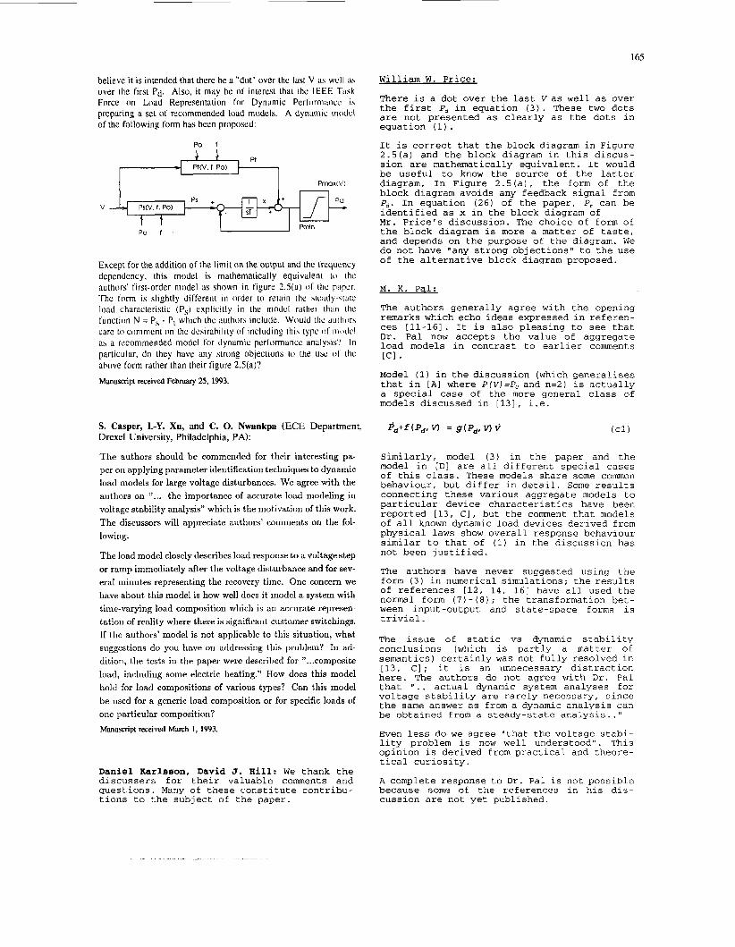
believe it is intended that there be a "dot" over the last V as well LIX

over the first Pd. Also, i t may be of interest that the IEEE Task Force on Load Representation for Dynamic Pcrl'orniancc i \ preparing a set of recommended load models. A dynamic modcl of the following form has been proposed:

PmoxW

Po f

Except for the addition of the limit on the output and the trequcncy dependency, this model is mathematically equivalent to the authors' first-order model as shown in figure 2.5(a) of thc papcr. The lorm is slightly different in order to retain the Stciidy-sIiitc load characteristic (P,) explicitly i n the modcl rather than the function N = P, - Pt which thc authors include. Would thc ilu[liorb care to comment on thc desirability oc including this typc OF iiie)dcI as a rccornmended model for dynamic performancc analysis'! I n particular, do they have any strong objections to the usc ol' the above form rather than their figure 2.5(a)? Manuscript received February 25, 1993.

S. Casper, L-Y. Xu, and C. 0. Nwankpa (ECE Department, Drexel University, Philadelphia, PA):

The authors should be commended for their interesting paper on applying parameter identification techniques to dynamic load models for large voltage disturbances. We agree with the authors on " ... the importance of accurate load modeling in voltage stability analysis" which is the motivation of this work. The discussors will appreciate authors' comments on the following.

The load model closely describes load response to a voltage step or ramp immediately after the voltage disturbance and for several minutes representing the recovery time. One concern we have about this model is how well does it model a system with time-varying load composition which is an accurate representation of reality where there is significant custoiner switchings. If the authors' model is not applicable to this situation, what suggestions do you have on addressing this problem? In addition, the tests in the paper were described for ''...composite load, including some electric heating." How does this model hold for load compositions of various types? Can this model be used for a generic load composition or for specific loads of one particular composition? Manuscript received March 1, 1993.

Daniel Karlseon, David J. Hill: We thank the discussers for their valuable comments and questions. Many of these constitute contribu- tions to the subject of the paper.

William W. Price:

There is a dot over the last Vas well as over the first Pd in equation (3). These two dots are not presented as clearly as the dots in equation (1).

It is correct that the block diagram in Figure 2.5(a) and the block diagram in this discussion are mathematically equivalent. It would be useful to know the source of the latter diagram. I n Figure 2.5(a), the form of the block diagram avoids any feedback signal from Pd. In equation (26) of the paper, P, can be identified as x in the block diagram of Mr. Price's discussion. The choice of form of the block diagram is more a matter of taste, and depends on the purpose of the diagram. We do not have "any strong objections" to the use of the alternative block diagram proposed.

M. K. Pal:

The authors generally agree with the opening remarks which echo ideas expressed in references [ll-161. It is also pleasing to see that Dr. Pal now accepts the value of aggregate load models in contrast to earlier comments [Cl.

Model (1) in the discussion (which generalises that in [AI where P ( V ) = P , and n=2) is actually a special case of the more general class of models discussed in [13], i.e.

Similarly, model (3) in the paper and the model in [D] are all different special cases of this class. These models share some common behaviour, but differ in detail. Some results connecting these various aggregate models to particular device characteristics have been reported [13, C ] , but the comment that models of all known dynamic load devices derived from physical laws show overall response behaviour similar to that of (1) in the discussion has not been justified.

The authors have never suggested using the form (3) in numerical simulations; the results of references [12, 14, 161 have all used the normal form (7) - (8) ; the transformation between input-output and state-space forms is trivial.

The issue of static vs dynamic stability conclusions (which is partly a matter of semantics) certainly was not fully resolved in [13, C]; it is an unnecessary distraction here. The authors do not agree with Dr. Pal that ' I . . actual dynamic system analyses for voltage stability are rarely necessary, since the same answer as from a dynamic analysis can be obtained from a steady-state analysis.."

Even less do we agree "that the voltage stability problem is now well understood". This opinion is derived from practical and theore- tical curiosity.

A complete response to Dr. Pal is not possible because some of the references in his discussion are not yet published.

.- . .

166

S. CasDer, L-Y. Xu, C. 0. NwankRa:

The disussers first question is about how well the proposed load model models a system with time-varying load composition, which originates from customer switchings. The answer is that the structure of the model is applicable for all the compositions investigated. The parameter values, however, differ for different times of the day and different times of the year. This means that the load model structure holds for time-varying load compositions, but the parameters have to be adjusted.

The second question is about how well the load model holds for load compositions of different types. The field measurements were performed in two different substations in the South of Sweden for different times of the year and different times of the day. One of the substations was feeding an "extremely" residential load composition, consisting of a village

with mainly one-family houses and no industry at all (about 10 000 households). The other substation was feeding a slightly smaller village including a quite big industry. The load model is accurate for all the recordings from these two substations. The active power recovery largely originates from thermostat controlled heating devices, which is a large part of the load during winter. The load model does not include induction machine dynamics or any other short term dynamics (time constants less than 10 seconds). It is the opinion of the authors that the structure of the proposed load model is valid for residential and com- mercial load compositions including some electrical heating. Induction machines and other specific load devices with certain characteristics have to be modelled separately, if they are a large part of the total load or if their behaviour is significant for the study. Manuscript received May 4, 1993.

Documents

Modelling and identification of nonlinear dynamic loads …mickgg/docs/Karlsson+Hill.pdf · MODELUNG AND IDENTIFICATION OF NONLINEAR DYNAMIC LOADS IN POWER SYSTEMS ... stability analysis