Electronic copy available at: http://ssrn.com/abstract=1484773

Modeling the Under Reporting Bias in Panel Survey Data

Sha Yang (NYU)1, Yi Zhao (HKUST) and Ravi Dhar (Yale)

Abstract

Panel survey data have been gaining importance in marketing. However, one challenge of

estimating econometric models based on panel survey data is how to account for underreporting, that is, respondents do not report behavioral incidences which actually occur. Underreporting is especially likely to occur in a panel survey because the data recording mechanism is often tedious, complex and effortful. The probability of underreporting is likely to vary across respondents and also over the duration of the survey period. In this paper, we propose a model to simultaneously study reported behavioral incidences and partially observed actual behavioral incidences. We propose a Bayesian approach for estimating the proposed model. We treat those unobserved actual behavioral incidences as latent variables, and the Gibbs Sampler makes it convenient to impute the non-reported consumption incidences along with making inferences on other model parameters. Our proposed method has two advantages. First, it offers a model-based approach to remove the underreporting bias in panel survey data, and therefore allows marketing researchers to make accurate inferences about consumers’ actual behavior. Second, the method also offers a natural way to study factors that influence respondents’ propensity to underreport. Since we treat those underreported behavioral incidences as non-missing-at-random (NMAR), this underreporting propensity varies across respondents and over time. This understanding can help marketing researchers design the right strategy to intervene and incentivize respondents to authentically report and hence improve the quality of survey data. The proposed model and estimation approach are tested on both synthetic data and an actual panel survey data on consumer reported beverage-drinking behavior. Our analysis suggests that underreporting can significantly mask respondents’ true behavior. Keywords: Panel Survey Data Analysis, Measurement Error, Underreporting, Bayesian Analysis

1 Corresponding Author: Sha Yang, Associate Professor of Marketing at New York University, shayang@stern.nyu.edu.

1

Electronic copy available at: http://ssrn.com/abstract=1484773

1. INTRODUCTION

Survey is a popular marketing research tool for collecting information on consumer attitudes

and behaviors. When it is difficult to directly observe consumer actions, marketers often rely on

surveys to have respondents report their behaviors over time and collect longitudinal panel survey data.

With the advent of new digital technology, the use of diary data is increasing. For example, advertising

research companies repeatedly collect media usage information from the same respondent for every

hour in an entire week. Beverage companies recruit participants to record their beverage consumption

on any drinking occasion in a given time period.

Panel survey data have two primary benefits compared with cross sectional survey data. First,

panel survey data allow marketers to collect micro-level information such as when consumption occurs

and what type of product is consumed in every consumption occasion. Such micro-level information

helps marketers gain more insights on consumer behavior. Second, panel survey data make it

convenient to study consumer behavioral dynamics. For example, diary data allow marketers to study

how past behaviors affect current behavior, which can be useful in many marketing research contexts

(Guadagni and Little 1983, Erdem and Keane 1996).

At the same time, collecting multi-day data creates the problem of underreporting if a

respondent’s ability and willingness to keep accurate recording declines over time (Kitamura and Bovy

1987), making it difficult to estimate econometric models. Underreporting has been documented

(Turner 1961, Waksberg and Neter 1965, Lee, Hu and Toh 2000) and modeled (Bailar 1975, Bollinger

and David 1997) in the literature. Imagine the following scenario where marketing researchers have

respondents make a record and answer a few consumption-related questions whenever consumption of

a product occurs for a two-week period. In such context especially when the survey involves a

frequently consumed product, underreporting is especially likely to occur because the data recording

2

mechanism is tedious, complex and effortful. Moreover, this underreporting probability is likely to

increase in the later stage of the longitudinal survey because respondents may feel less involved in the

task. Finally, this underreporting probability is likely to vary across respondents because of the

heterogeneity in their ability or wiliness to accurately report and consumption patterns.

If underreporting occurs, it would be difficult to study respondents’ true behavior based on

reported panel survey data. For example, if we find women tend to drink soft drinks less often than

men, it could be due to the gender difference in consumption propensity and/or because women are

more likely to underreport than men when participating in the longitudinal survey. What becomes more

problematic is when estimating the state-dependence effect in the consumption, i.e. the effect of last

period consumption incidence on the current period consumption utility. Since last period consumption

incidence is measured with error, the state-dependence effect is likely to be biased if such omission

error is not accounted for.

In this paper, we address these aforementioned challenges by proposing a model to

simultaneously study reported behavioral incidences and partially observed true behavioral incidences.

Given the complexity of the proposed model, we propose a Bayesian estimation approach. The essence

of the proposed estimation method is to treat the actual behavioral incidences as latent variables, and

the Gibbs Sampler makes it convenient to impute these non-reported consumption incidences along

with making inferences on other model parameters. The proposed model and estimation approach are

tested on both synthetic data and an actual panel survey data on consumer reported beverage

consumption behavior. Our analysis suggests that underreporting can significantly mask respondents’

true behavior.

Our proposed model has two important managerial implications. First, it offers a model-based

approach to remove the underreporting bias in panel survey data, and therefore allows marketing

3

researchers to make accurate inferences about consumer behavior. Our empirical analysis with both

simulated and actual data suggests that it is important to control for the underreporting to avoid biased

inferences. Second, our model offers a natural way to study the factors that influence a respondent’s

propensity to underreport. Since we treat those underreported behavioral incidences as non-missing-at

-random (NMAR), this underreporting propensity varies across respondents and over time. This

understanding can help marketing researchers design the right strategy to intervene and incentivize

respondents to accurately report, and therefore improve the quality of panel survey data.

The remainder of this paper is organized as follows. We will next review the relevant literature

on data measurement in panel survey data. We then propose a model and a Bayesian estimation

approach to study the underreporting behavior. We then apply the proposed model to a panel survey

dataset collected by a large beverage manufacturer on consumer beverage consumption behavior, and

discuss the empirical findings. We conclude the paper with a brief summary and potential extensions of

our study.

2. LITERATURE REVIEW

Studies describing response error with consumer survey data in marketing can be dated back to

1960’s. Sudman (1964) documented the accuracy of consumer panel data and studied the determining

factors. Mandell and Lundsten (1978) provided evidence of underreporting of financial data by survey

respondents because high asset households may consistently underestimate their asset holdings.

Hawkins and Coney (1981) documented the uninformed response error in survey research and

examined factors that influence respondents’ tendency to make an uninformed response. There has

been abundant evidence in the literature suggesting biases in survey results of behavioral frequency,

and marketing researchers have examined factors attributing to these biases and ways to reduce biases

4

with improved questions (Menon 1993, 1997). Lee, Hu and Toh (2000) investigated how actual

behavioral frequency and duration systematically affect the direction of errors in consumer survey

responses. They demonstrate that high-frequency groups underreported their behavioral frequencies,

whereas low-frequency groups overreported them. While actual usage data are accessible in those

aforementioned studies, they are not readily available in many other cases such as consumption

incidence, creating a challenge to determine the magnitude of the response error. Our paper extends

this line of literature by proposing a modeling framework to study the actual behavioral incidence and

the underreporting mechanism simultaneously.

Our research is methodologically related to some work in statistics on modeling discrete choice

with response error in cross-sectional survey data. For example, Bradlow and Zaslavsky (1999)

modeled the “no answer” responses in customer satisfaction survey. Bollinger and David (1997)

studied the omission and commission error in the reported food stamp participation. Our study differs

and extends this line of work in the following two ways. First, unlike these prior studies that focused

on cross-sectional self-reported data, we study panel study data with the state dependence effect. The

impact of last period behavioral incidence on the current period utility, i.e. the state dependence effect,

is an important element to include when modeling panel data. As we show later, estimating state

dependence effect adds additional complexity in the analysis of panel survey data with response error,

and it is difficult to estimate such model with traditional estimation approaches. To the best of our

knowledge, we are the first to incorporate state dependence effect in analyzing longitudinal panel

survey data while correcting for the underreporting bias. Second, in our proposed framework, we

simultaneously model the factors that drive true behavioral incidence and the underreporting

likelihood. Consequently, such model allows researchers to disentangle the effect of the same covariate

on respondents’ true behavior and their likelihood of underreporting.

5

In the Statistics literature, researchers have modeled the phenomenon that the likelihood of

underreporting is likely to increase over time as the respondent loses interest and incentive in

longitudinal panel surveys. The common approach to statistically control for such effect is to model the

dependent variable (continuous or discrete) as a function of explanatory covariates and a time trend

(See Fuller 1995 for a discussion). This approach has several limitations. First, this approach assumes

that there is no underreporting in the first period, which is a strong assumption. Second, the time trend

specification does not allow researchers to disentangle the dynamics from the reporting behavior and

the dynamics from the actual behavior. For example, the observation that reported consumption

frequency decreases over the survey period can be driven by that respondents are underreporting

towards the later stage and/or respondents are indeed drinking less due to the seasonal variation. Third,

since the underlying process of underreporting is not modeled in this standard approach, researchers

are not able to disentangle the effect of the same covariate on the respondent’s true consumption

behavior and on the respondent’s underreporting tendency. Finally, it will be very difficult, if at all

possible, to model the state-dependence in true consumption behavior, with this standard approach.

This is because lagged reported consumption incidence is measured with error and this measurement

error needs to be statistically controlled. The goal of this paper is to propose a model to address these

aforementioned limitations.

Finally, our research is related to marketing studies on response style. Ter Hofstede, Steenkamp

and Wedel (1999) modeled the response scale usage in their market segmentation research. Rossi,

Gilula and Allenby (2001) addressed the issue that respondents vary in their scale usage when

answering survey questions, and proposed a statistical model with individual scale and location effects

to capture scale usage differences. Bradlow, Hu and Ho (2004a) developed a learning-based

imputation model to study how respondents infer missing levels of product attributes in conjoint

6

studies with partial conjoint profiles. Gilbride, Yang and Allenby (2005) proposed a modeling

approach and empirically showed how brand usage and attribute perception responses are jointly

determined by justification, order, and brand halo effects. Baumgartner and Steenkamp (2001)

examined five forms of stylistic responding (acquiescence and disacquiescence response styles,

extreme response style/response range, midpoint responding, and noncontingent responding) and

discussed their biasing effects on scale scores and correlations between scales. De Jong et al. (2008)

studied the extreme response style in marketing research using item response theory. Marketing

researchers have examined how fatigue can affect respondent’s choice behavior in conjoint studies

(Otter, Frühwirth-Schnatter and Tüchler 2003, Liechty, Fong, and DeSarbo 2005), and attrition biases

in dairy panel (Toh and Hu 1996). Researchers have also studied social desirability response style and

how to control for social desirability bias in survey research (Ganster, Hennessey, and Luthans 1983,

Fisher 1993, Myung-soo, Nelson and Kiecker 1997, De Jong, Pieters and Fox 2009). Our study

complements this line of research by modeling one type of response style, underreporting, in the

context of longitudinal panel survey research. In the following section, we lay out the model, describe

how to estimate the proposed model using MCMC with data augmentation, and test the proposed

model and estimation approach with synthetic data.

3. MODEL

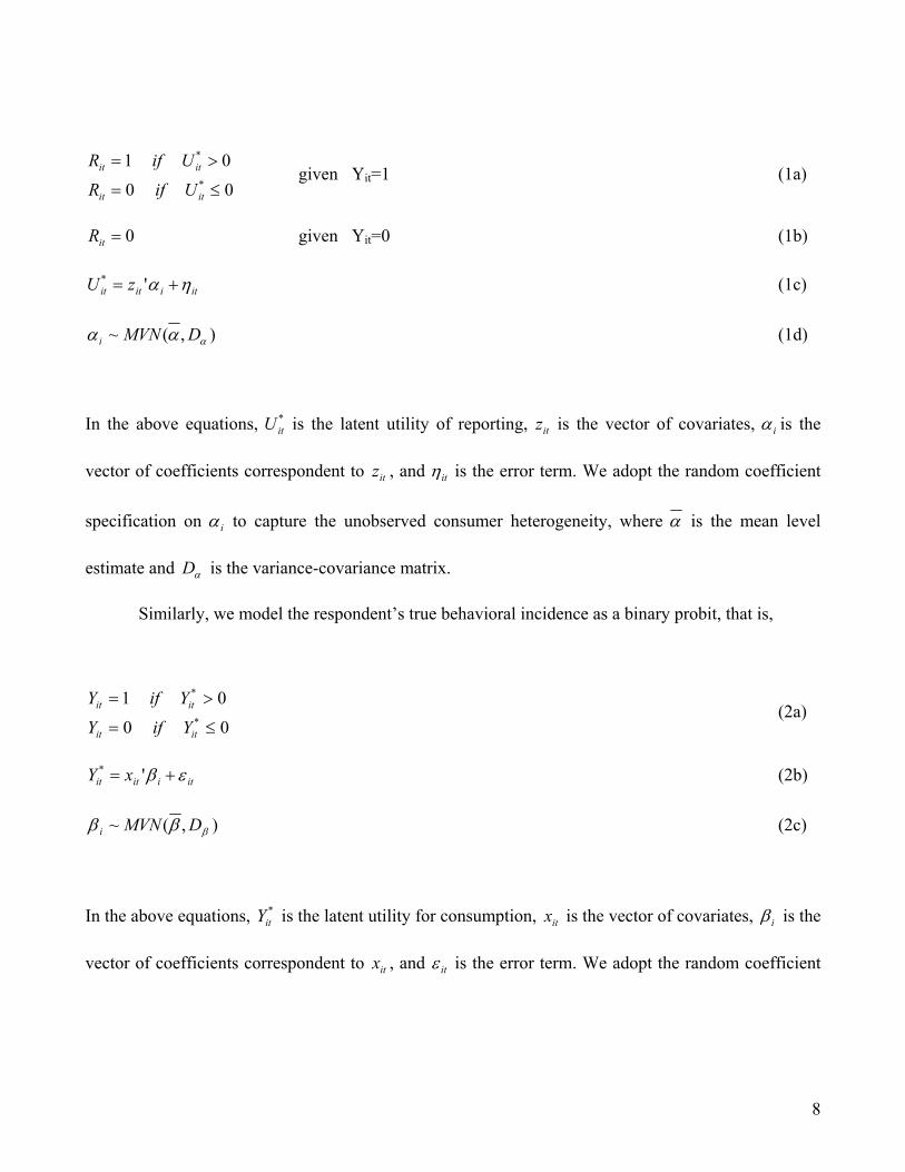
Let Rit stand for the reported incidence of a behavior and Yit stand for the actual incidence of a

behavior (such as consumption of a product) by respondent i at time t in the survey period. When

underreporting happens, some actual behavioral incidences are not reported. The econometrician only

observes Rit. When a behavior occurs (Yit=1), we model the respondent’s decision on whether to report

or not to report as in a standard binary probit setting, that is,

7

00

01

≤=

>=*itit

*itit

U if R

U if R given Yit=1 (1a)

0=itR given Yit=0 (1b)

itiit*it zU ηα += ' (1c)

),(~ ααα DMVNi (1d)

In the above equations, U is the latent utility of reporting, z is the vector of covariates, *it it iα is the

vector of coefficients correspondent to , and itz itη is the error term. We adopt the random coefficient

specification on iα to capture the unobserved consumer heterogeneity, where α is the mean level

estimate and is the variance-covariance matrix. αD

Similarly, we model the respondent’s true behavioral incidence as a binary probit, that is,

00

01

≤=

>=*

itit

*itit

Y if Y

Y if Y (2a)

itiit*

it xY εβ += ' (2b)

),(~ βββ DMVNi (2c)

In the above equations, Y is the latent utility for consumption, is the vector of covariates, *it itx iβ is the

vector of coefficients correspondent to , and itx itε is the error term. We adopt the random coefficient

8

specification on iβ to capture the unobserved consumer heterogeneity, where β is the mean level

estimate and is the variance-covariance matrix. βD

ρ

MVN

00

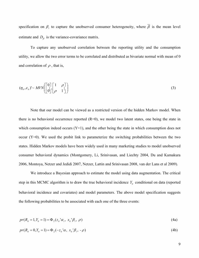
To capture any unobserved correlation between the reporting utility and the consumption

utility, we allow the two error terms to be correlated and distributed as bivariate normal with mean of 0

and correlation of , that is,

1

1,~)',(ρ

ρεη

itit (3)

Note that our model can be viewed as a restricted version of the hidden Markov model. When

there is no behavioral occurrence reported (R=0), we model two latent states, one being the state in

which consumption indeed occurs (Y=1), and the other being the state in which consumption does not

occur (Y=0). We used the probit link to parameterize the switching probabilities between the two

states. Hidden Markov models have been widely used in many marketing studies to model unobserved

consumer behavioral dynamics (Montgomery, Li, Srinivasan, and Liechty 2004, Du and Kamakura

2006, Montoya, Netzer and Jedidi 2007, Netzer, Lattin and Srinivasan 2008, van der Lans et al 2009).

We introduce a Bayesian approach to estimate the model using data augmentation. The critical

step in this MCMC algorithm is to draw the true behavioral incidence Y conditional on data (reported

behavioral incidence and covariates) and model parameters. The above model specification suggests

the following probabilities to be associated with each one of the three events:

it

),','()1,1( 2 ρβα x zYRpr iitiititit Φ=== (4a)

),','()1,0( 2 ρβα - x zYRpr iitititit −Φ=== (4b)

9

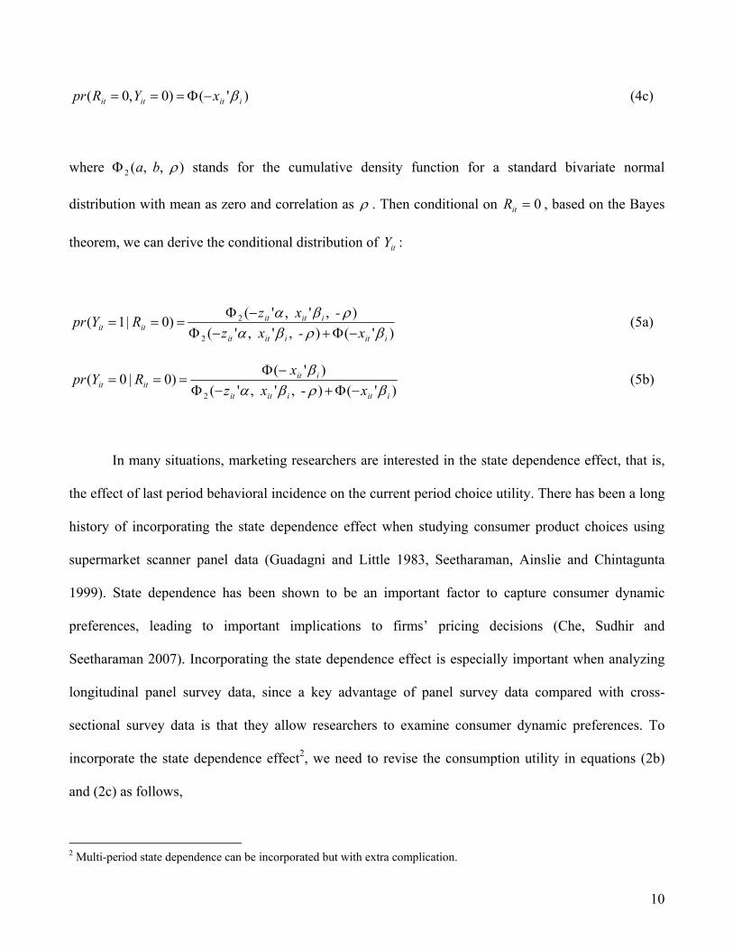
)'()0,0( iititit xYRpr β−Φ=== (4c)

where ),,(2 ρ b aΦ stands for the cumulative density function for a standard bivariate normal

distribution with mean as zero and correlation as ρ . Then conditional on R , based on the Bayes

theorem, we can derive the conditional distribution of Y :

0=it

it

)'(),','(),','()0|1(

2

2

iitiitit

iitititit x- x z

- x zRYprβρβα

ρβα−Φ+−Φ

−Φ=== (5a)

)'(),','()'()0|0(

2 iitiitit

iititit x- x z

x RYprβρβα

β−Φ+−Φ

−Φ=== (5b)

In many situations, marketing researchers are interested in the state dependence effect, that is,

the effect of last period behavioral incidence on the current period choice utility. There has been a long

history of incorporating the state dependence effect when studying consumer product choices using

supermarket scanner panel data (Guadagni and Little 1983, Seetharaman, Ainslie and Chintagunta

1999). State dependence has been shown to be an important factor to capture consumer dynamic

preferences, leading to important implications to firms’ pricing decisions (Che, Sudhir and

Seetharaman 2007). Incorporating the state dependence effect is especially important when analyzing

longitudinal panel survey data, since a key advantage of panel survey data compared with cross-

sectional survey data is that they allow researchers to examine consumer dynamic preferences. To

incorporate the state dependence effect2, we need to revise the consumption utility in equations (2b)

and (2c) as follows,

2 Multi-period state dependence can be incorporated but with extra complication.

10

ittiiiit*

it YxY εδβ ++= −1,' (6a)

),(~]','[ θθδβθ DMVNiii = (6b)

Incorporating state dependence effect is standard when there is no measurement error on last

period behavioral incidence. However, when last period behavioral incidence is measured with error,

we need to account for this measurement error. Now, in order to draw Y with the state dependence

effect incorporated, we need to derive the probability of each of the nine possible combinations of

outcomes conditional on Y .

it

1, −ti

),','(),','()1,1,1,0Pr(

1,1,21,2

1,1,

ρδβαρδβα iitiititiiiitiit

titiitit

xzYxzYRYR

+Φ×−+−Φ=

====

++−

++ (7a)

),','(),','()1,0,1,0Pr(

1,1,21,2

1,1,

ρδβαρδβα −+−Φ×−+−Φ=

====

++−

++

iitiititiiiitiit

titiitit

xzYxzYRYR

(7b)

)]'(1[),','()0,0,1,0Pr(

1,1,2

1,1,

iititiiiitiit

titiitit

xYxzYRYR

δβρδβα +Φ−×−+−Φ=

====

+−

++ (7c)

),','()]'(1[)1,1,0,0Pr(

1,1,21,

1,1,

ρβαδβ itiititiiiit

titiitit

xzYxYRYR

++−

++

Φ×+Φ−=

==== (7d)

),','()]'(1[)1,0,0,0Pr(

1,1,21,

1,1,

ρβαδβ −−Φ×+Φ−=

====

++−

++

itiititiiiit

titiitit

xzYxYRYR

(7e)

)]'(1[)]'(1[)0,0,0,0Pr(

1,1,

1,1,

ititiiiit

titiitit

xYxYRYR

βδβ +−

++

Φ−×+Φ−=

==== (7f)

),','(),','()1,1,1,1Pr(

1,1,21,2

1,1,

ρδβαρδβα iitiititiiiitiit

titiitit

xzYxzYRYR

+Φ×+Φ=

====

++−

++ (7g)

11

),','(),','()1,0,1,1Pr(

1,1,21,2

1,1,

ρδβαρδβα −+−Φ×+Φ=

====

++−

++

iitiititiiiitiit

titiitit

xzYxzYRYR

(7h)

)]'(1[),','()0,0,1,1Pr(

1,1,2

1,1,

iititiiiitiit

titiitit

xYxzYRYR

δβρδβα +Φ−×+Φ=

====

+−

++ (7i)

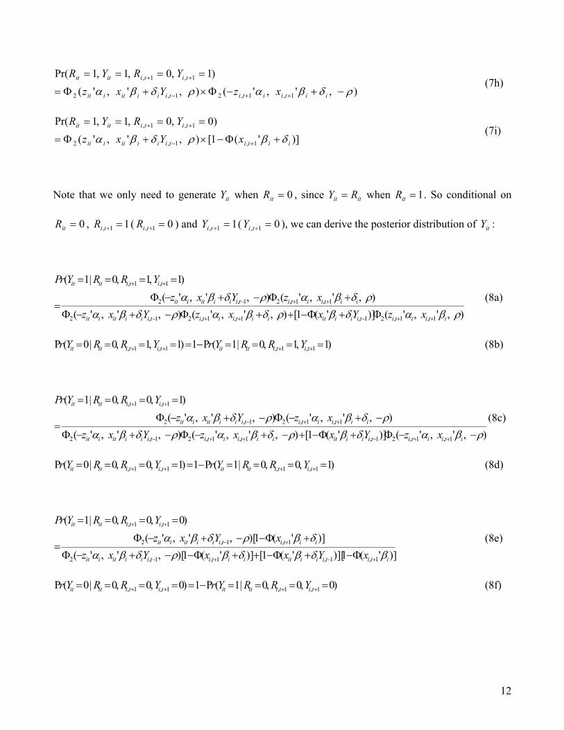
Note that we only need to generate Y when it 0=itR , since Y itit R= when . So conditional on

, ( ) and Y ( 0

1=itR

0=itR 11, =+tiR 01, =+tiR 1, +ti 1 = 1, =+tiY ), we can derive the posterior distribution of Y : it

),','()]'(1[),','(),','(),','(),','(

)1,1,0|1(

1,1,21,1,1,21,2

1,1,21,2

1,1,

ρβαδβρδβαρδβαρδβαρδβα

itiititiiiitiitiititiiiitiit

iitiititiiiitiit

titiitit

xzYxxzYxzxzYxz

YRRYrP

++−++−

++−

++

Φ+Φ−++Φ−+−Φ

+Φ−+−Φ=

====

(8a)

)1,1,0|1(P1)1,1,0|0(P 1,1,1,1, ====−===== ++++ titiitittitiitit YRRYrYRRYr (8b)

),','()]'(1[),','(),','(),','(),','(

)1,0,0|1(

1,1,21,1,1,21,2

1,1,21,2

1,1,

ρβαδβρδβαρδβαρδβαρδβα

−−Φ+Φ−+−+−Φ−+−Φ

−+−Φ−+−Φ=

====

++−++−

++−

++

itiititiiiitiitiititiiiitiit

iitiititiiiitiit

titiitit

xzYxxzYxzxzYxz

YRRYrP(8c)

)1,0,0|1(P1)1,0,0|0(P 1,1,1,1, ====−===== ++++ titiitittitiitit YRRYrYRRYr (8d)

)]'(1)]['(1[)]'(1)[,','()]'(1)[,','(

)0,0,0|1(

1,1,1,1,2

1,1,2

1,1,

ititiiiitiititiiiitiit

iititiiiitiit

titiitit

xYxxYxzxYxz

YRRYrP

βδβδβρδβαδβρδβα

+−+−

+−

++

Φ−+Φ−++Φ−−+−Φ

+Φ−−+−Φ=

====

(8e)

)0,0,0|1(P1)0,0,0|0(P 1,1,1,1, ====−===== ++++ titiitittitiitit YRRYrYRRYr (8f)

12

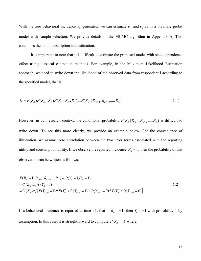
With the true behavioral incidence Y generated, we can estimate it iα and iθ as in a bivariate probit

model with sample selection. We provide details of the MCMC algorithm in Appendix A. This

concludes the model description and estimation.

It is important to note that it is difficult to estimate the proposed model with state dependence

effect using classical estimation methods. For example, in the Maximum Likelihood Estimation

approach, we need to write down the likelihood of the observed data from respondent i according to

the specified model, that is,

),...,,|()....,|()|()( 12,1,123121 RRRRPRRRPRRPRPL TiTiiTiiiiiii −−= (11)

However, in our research context, the conditional probability P is difficult to

write down. To see this more clearly, we provide an example below. For the convenience of

illustration, we assume zero correlation between the two error terms associated with the reporting

utility and consumption utility. If we observe the reported incidence

),...,,|( 12,1, ititiit RRRR −−

1=itR , then the probability of this

observation can be written as follows:

[ ])0|0(*)0()1|0(*)1()'(

)1()'()1,1(),...,|1(

1,*

1,1,*

1,

12,1,

=>=+=>=Φ=

=Φ=

====

−−−−

−−

tiittitiittiiit

itiit

ititititiit

YYPYPYYPYPZ

YPZUYPRRRRP

α

α (12)

If a behavioral incidence is reported at time t-1, that is 11, =−ti

)1(

R , then Y with probability 1 by

assumption. In this case, it is straightforward to compute

11, =−ti

=itRP where,

13

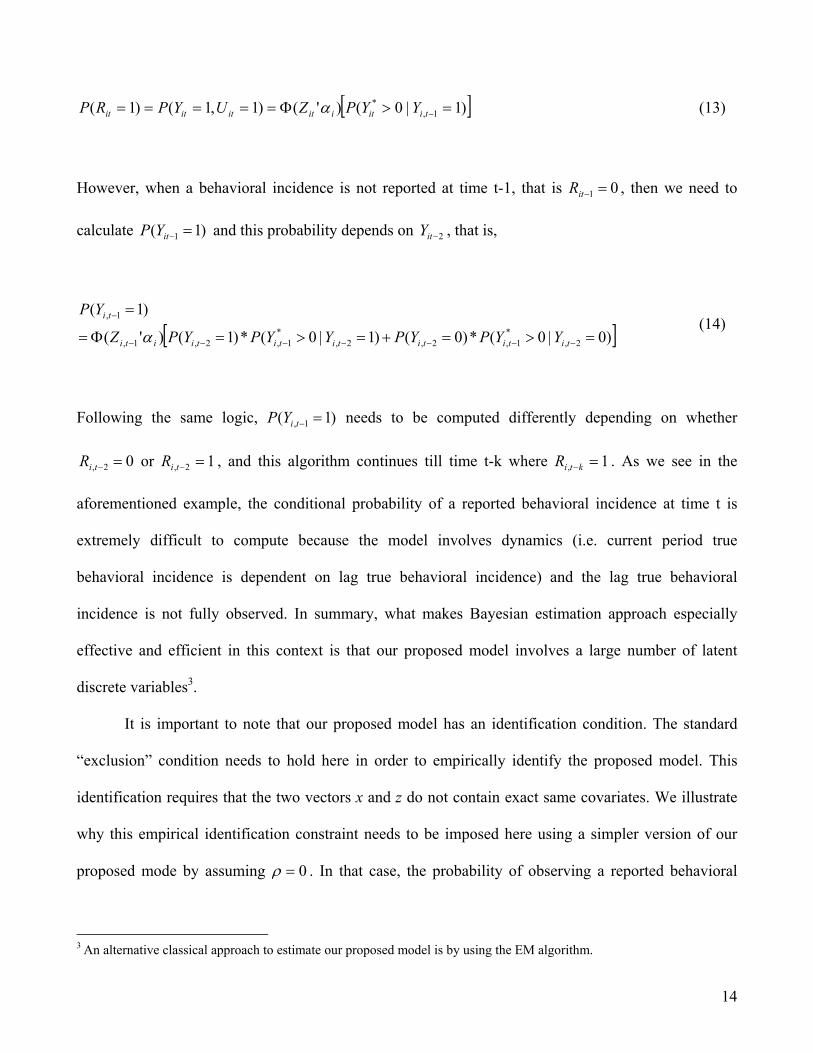
[ ])1|0()'()1,1()1( 1,* =>Φ===== −tiitiitititit YYPZUYPRP α (13)

However, when a behavioral incidence is not reported at time t-1, that is R , then we need to

calculate and this probability depends on Y , that is,

01 =−it

)1( 1 =−itYP 2−it

[ ])0|0(*)0()1|0(*)1()'(

)1(

2,*

1,2,2,*

1,2,1,

1,

=>=+=>=Φ=

=

−−−−−−−

−

titititititiiti

ti

YYPYPYYPYPZ

YP

α (14)

Following the same logic, P needs to be computed differently depending on whether

or , and this algorithm continues till time t-k where R . As we see in the

aforementioned example, the conditional probability of a reported behavioral incidence at time t is

extremely difficult to compute because the model involves dynamics (i.e. current period true

behavioral incidence is dependent on lag true behavioral incidence) and the lag true behavioral

incidence is not fully observed. In summary, what makes Bayesian estimation approach especially

effective and efficient in this context is that our proposed model involves a large number of latent

discrete variables

)1( 1, =−tiY

02, =−tiR 12, =−tiR 1, =−kti

3.

It is important to note that our proposed model has an identification condition. The standard

“exclusion” condition needs to hold here in order to empirically identify the proposed model. This

identification requires that the two vectors x and z do not contain exact same covariates. We illustrate

why this empirical identification constraint needs to be imposed here using a simpler version of our

proposed mode by assuming 0=ρ . In that case, the probability of observing a reported behavioral

3 An alternative classical approach to estimate our proposed model is by using the EM algorithm.

14

incidence (Rit=1) is )'()'( iitiit xz βα Φ

'()'( itiit xz

Φ and the probability of not observing a reported behavioral

incidence (Rit=0) is 1- )iβα ΦΦ . If z itit x= , then different combinations of iα and iβ can

lead to the same likelihood of the data. There are two suggestions on how to impose the “exclusion”

identification constraint. First, we can include a set of covariates in the consumption utility function

but include only an intercept in the reporting utility function. This specification usually serves the

purpose of testing whether underreporting exists in the data. Second, behavioral theory and previous

findings can help us find variables that only predict one but not the other. For example, some

psychographic variables such as consumer general attitudes towards survey participation can predict

the authentic reporting probability but not necessarily the true consumption incidence.

To test the proposed model, we have conducted simulation analysis. We have simulated data

according to the proposed model with pre-specified parameter values, and then estimated these

parameters using the proposed method. Our results suggest that our estimation approach can recover

the true parameter values of the proposed model. In addition, our simulations fulfill other two

important goals. First, it helps us determine whether the model is statistically identified. Second, it

helps us quantify the direction and size of the biases on model parameters caused by the underreporting

response style. Overall, our simulation results show that the proposed model is identified, the proposed

estimation method works well on recovering true parameter values, and ignoring the underreporting

phenomenon leads to biased inferences. For details of the simulation, please refer to Appendix B.

4. AN EMPIRICAL APPLICATION

4.1 Data and Variable Specification

The data were provided to us by one of the world’s leading marketers of non-alcoholic

beverages, who collect these data as part of an extensive and ongoing market research exercise lasting

15

several years. Each respondent was provided with a handheld personal digital assistant. In each

weekday over a two-week period, a respondent was asked to make a record and answer a few

consumption-related questions whenever he/she consumed a beverage at that moment. Underreporting

is likely to occur in such context. Since the data recording mechanism is tedious, complex and effortful,

it is possible that consumption occurs but a respondent does not record the behavioral incidence. On

the other hand, overreporting is less likely to occur in such context based on the same intuition.

We randomly sampled 1000 respondents surveyed in the three months of June, July and August

in 2003 for our empirical analysis. For each respondent, and for each of the six day-parts (morning,

lunch, afternoon, dinner, night, late night) on each of the ten days, we created a dummy variable

indicating whether the person reports any beverage consumption. Figures 1a, 1b and 1c plot the total

daily consumption frequency from the 1000 respondents over ten days of the survey period for

beverage overall and two specific types of beverage: water and soft drink. Regression analysis on the

ten data points suggests a negative and significant time trend for all three categories. This provides

evidence of underreporting since consumer consumption frequency on these product categories is

unlikely to be changing significantly during a two-week period.

= = Insert Figure 1a, Figure 1b and Figure 1c Here = =

Next, we discuss the details of the model specification. In the consumption utility, we include

eight variables that capture a respondent’s demographics, psychographics and time effect: AGE,

GENDER, EDUCATION, INCOME, LOOKGOOD, INDULGE, HEALTHY and LOG_WEEK. The

coefficients of these variables are modeled with fixed effects. AGE is measured as a respondent’s

actual age. GENDER = 0 for males and GENDER = 1 for females. EDUCATION is measured on the

following 6-point scale: 1=grade school or less; 2=some high school, 3=high school graduate; 4=some

college or trade school; 5=college graduate; 6=post graduate work. INCOME was measured on the

16

following 7-point scale: 1=under $15,000; 2=$15,000-$25,000; 3=$25,000-$35,000; 4=$35,000-

$50,000; 5=$50,000-$75,000; 6=$75,000-$100,000; 7=$100,000 or greater. Respondents also reported

the level of the motivation for looking good (LOOKGOOD) which is measured on a 3-point scale

(1=least, 2=average, 3=most), the likelihood of being motivated by indulging oneself (INDULGE), and

the likelihood of being motivated to be healthy (HEALTHY). The likelihood measure ranges from 0 to

1. Since the 1000 randomly sampled respondents were surveyed for a two-week period at different

time points during the three months, we include LOG_WEEK variable that is measured by the natural

log of the week (from 1 to 12 since we have data from 12 consecutive weeks in those three months) of

a respondent’s reported consumption incidences. This potentially captures the beverage consumption

dynamics due to change of weather (becoming hotter in our context). In the consumption utility, we

also include seven variables that are modeled with random coefficients or unobserved heterogeneity

across respondents: the six day-parts (MORNING, LUNCH, AFTERNOON, DINNER, NIGHT, LATE

NIGHT) and lagged actual consumption incidence to capture the state dependence effect. Note that the

“exclusion” identification constraint is imposed by including the ten day dummies in the reporting

utility while including LOG_WEEK in the consumption utility.

We estimated fixed effects for all the covariates included in the utility of reporting conditional

on a consumption incidence4. These covariates include the seven demographic and psychographic

variables as mentioned above, ten dummies to indicate the consumption in any of the ten days of the

survey period, and the six day-parts as mentioned above where LATE NIGHT is treated as the baseline.

In order to ensure the convergence of the mcmc chain, we adopted three different techniques to

test the convergence. First, we did the time series inspection on trace plots, which has been often used

in the marketing literature. Second, we computed the Geweke convergence diagnostic (1992), which

4 The fixed effects specification leads to a better out-sample fit than the random coefficients specification for the reporting equation in our empirical application.

17

takes two non-overlapping parts of the Markov chain and compares the means of both parts, using a

difference of means test to assess if the two parts of the chain are from the same distribution (null

hypothesis). Lastly, we employed three sets of starting values for the model parameters, and the

moments of the posterior distributions remain unchanged across all sets. All three of these tests

indicated that model estimation is convergent.

4.2 Estimation Results

Table 1 reports the estimation results on consumption incidence of any beverage from both the

proposed model accounting for underreporting and the naïve model not accounting for underreporting.

We first discuss results from the proposed model. With regard to consumption utility, we find that the

consumption incidence varies from the lowest to the highest over the six day-parts in the following

order: late night, night, morning, afternoon, dinner and lunch. The state-dependence parameter at the

mean level is significantly negative (-0.209). The variance (heterogeneity) of the state dependence

parameter is 0.368, or its standard deviation is 0.607. This suggests that some respondents have a

positive state dependence coefficient whereas some respondents have a negative state dependence

coefficient. We also find significant unobserved heterogeneity in consumer beverage consumption

incidence over the six day-parts. On the effect of demographics, we find that females drink any

beverage more often than males. On the effect of psychographics, we find people who are more

motivated by INDULGE and HEALTHY drink beverages more frequently. Finally, the effect of LOG-

WEEK is insignificant.

On respondents’ reporting behavior conditional on consumption, our analysis reveals some

interesting findings. First, on the effects of demographic variables, we find that older respondents are

more likely to report and females are less likely to report than males when consumption occurs. Second,

on the effects of psychographic variables, we find that people who are more motivated by INDULGE

18

are less likely to report when consumption occurs. Third, the estimates on DAY1 through DAY10 show

that the reporting tendency is much lower in the last eight days than in the first two days, which may

be due to a decreased interest in expending the effort required. Fourth, the reporting tendency varies

over the six day-parts from the lowest to the highest in the following order: morning, afternoon, lunch,

late night, and night. This order is not consistent with that of the predicted consumption incidence,

which suggests that low (high) probability of a consumption incidence does not necessarily mean low

(high) reporting probability. The analysis on respondents’ authentic reporting behavior allows

marketing researchers to better understand who at what time are more likely to omit reporting of their

actual behavioral incidence. Finally, we find that there is a significant negative correlation between the

consumption utility and the reporting utility due to the unobserved variables in these two equations.

Next, we estimated a model where we treat the reported consumption incidence as the actual

consumption incidence without accounting for the possibility of omission. Estimates from such naïve

model are reported in the last two columns of Table 1. We find that failure of accounting for

underreporting leads to substantial biases in the coefficient estimates on the day-parts such as morning,

afternoon, night and late night. In addition, we find that the state dependence estimate is attenuated

towards zero (40% less negative in our case), consistent with our findings in the simulation.

= = Insert Table 1 Here = =

We have also estimated the same proposed model on soft drink consumption and water

consumption respectively. The estimates from both the proposed model and the native model on soft

drink consumption are reported in Table 2. Similarly, we find biases in estimates if not accounting for

underreporting. For example, our proposed model suggests that EDUCATION does not predict soft

drink consumption incidence, but according to the naïve model without accounting for the

underreporting bias, EDUCATION has a significant and positive effect. In the proposed model,

19

INCOME is found to have a significant and negative effect on soft drink consumption, but the naïve

model found the income effect to be insignificant. Interestingly, we find a significant and positive

effect of LOG_WEEK in the proposed model, suggesting that consumers consume soft drink more

frequently as weather turns hotter. However, the naïve model fails to detect this relationship. Finally,

apart from those estimates that suffer from a directional bias, we also find substantial biases on other

model parameters. For example, the effect of AGE on soft drink consumption utility is –0.261 (–0.089)

in the proposed (naive) model. The effect of INDULGE on soft drink consumption utility is 0.700

(0.345) in the proposed (naive) model. The mean level estimates on some of the six day-parts are

substantially biased. The variance (unobserved heterogeneity) estimates of the six day-part random

coefficients and the state dependence effect are underestimated in general.

= = Insert Table 2 Here = =

The estimates from both the proposed model and the native model on water consumption are

reported in Table 3. As shown in Table 3, the estimates on DAY1 through DAY10 in the report utility

from the proposed model are larger than those found in the overall beverage consumption. This

suggests that respondents have a higher probability of reporting when consuming water than when

consuming any beverage, leading to a lesser bias from the naïve model. However, there are still

significant biases when underreporting is not accounted for. For example, age is found to have a

significant and negative effect in water consumption in the proposed model, but found to have an

insignificant effect in the naïve model.

= = Insert Table 3 Here = =

In summary, as empirically demonstrated in the above three examples, it is important to model

the underreporting bias when respondents have a tendency to omit reporting but a behavior of interest

indeed occurs. Ignoring such underreporting bias can lead to wrong and/or inaccurate estimates of

20

model parameters. In this regard, our proposed model presents a modeling framework to correct such

bias. To gain more managerial insights, we compare the effect of same variables on consumption and

reporting of soft drink and water in Table 4, estimated from the proposed model.

= = Insert Table 4 Here = =

On the consumption utility, we find the following different and similar effects on the two

beverage categories: (i) Effect of demographics. Age has a negative effect for both soft drink (-0.199)

and water (-0.074). Females are predicted to drink soft drink (water) less (more) frequently than males.

INCOME has a significant and negative effect on soft drink consumption, but an insignificant effect on

water consumption incidence. (ii) Effect of psychographics. Specifically, we find that people who are

more motivated by LOOKGOOD and HEALTHY tend to consume soft drink less frequently and water

more frequently, and vice versa for those who are more motivated by INDULGE. (iii). Effect of

consumption dynamics. Interestingly, we find a positive (negative) consumption dynamics in soft drink

(water), suggesting that consumers tend to drink soft drink (water) more (less) often as weather turns

hotter. The magnitude of state dependence is about the same for these two types of beverages. (iv).

Mean level effect of day-parts. The predicted mean level consumption probability of soft drink and

water varies over the six day-parts in different patterns. For example, soft drink is consumed most in

lunchtime, whereas water is consumed most in afternoon. (v). Unobserved heterogeneity. In general,

we find that the variance of the random coefficients of day-parts and state dependence is larger in

consumption of soft drink than in consumption of water.

More importantly, our proposed model presents a modeling framework to allow marketing

researchers to better understand who are more likely to underreport and when underreporting is more

likely to occur. On the reporting utility, we find the following different and similar effects on the two

beverage categories: (i) Effect of demographics. For both categories of beverage, we find AGE has a

21

positive effect on the utility of reporting with the effect size being significantly larger for water. For

water, we find that females are less likely to report than males. For soft drink, we find that respondents

with higher income are more likely to report than respondents with lower income. (ii) Effect of

psychographics. We find that people with stronger consumption motivation of INDULGE are more

likely to underreport actual consumption incidence of both categories of beverage. (iii). Effect of

reporting dynamics. For both categories, we find the probability of reporting decreases over the 10-day

survey period. This pattern is consistent with the plots of consumption frequency observed in the data

shown in Figures 1a-1c, suggesting that the observed consumption dynamics from the data are likely

driven by the dynamics in the probability of reporting/underreporting. (iv). Effect of day-parts. The

probability of reporting is fairly constant across the six day-parts for both categories. (v). Unobserved

correlation. The correlation of the consumption utility and the reporting utility caused by the

unobservable is negative for both soft drink and water.

4.3 Model Validation

We next do model validation. Model validation is especially important in our context since

respondents’ true consumption behavior is not observed. To gain confidence in our proposed model

and the importance of correcting for the under-reporting bias, we provide both internal and external

validations.

For the internal validation, we conducted two sets of analysis. First, we compared our proposed

model with a naïve model that ignores underreporting, in predicting the reported consumption

incidence. The naïve model is a nested version or special case of our proposed model by assuming the

underreporting probability is zero. Table 5a reports the mean absolute deviation (MAD) between the

predicted probability of a reported consumption incidence and the actual reported consumption

22

incidence on any beverage, soft drink and water respectively. We found that our proposed model

predicts better for both in-sample and out-sample on all three categories.

Second, we ran correlation analysis between the predicted consumption incidence and the

actual consumption incidence. In our context, the company also collected an overall measure of how

frequently each respondent consumes each type of beverages overall (“FREQ”), which is measured on

a 5-point scale where “1” means least frequently and “5” means most frequently. This overall measure

is collected only once for each respondent and therefore is less prone to a systematic underreporting

bias. We use this measure to approximate a respondent’s actual consumption frequency. We found that

the correlation between “FREQ” and the predicted consumption incidence based on our proposed

model is 30% larger than the correlation between “FREQ” and the predicted consumption incidence

based on the naïve model. Collectively, these results suggest that our proposed model more accurately

predicts the reported consumption incidence and the actual consumption frequency.

= = Insert Table 5a Here = =

For the external validation, we collected new data (cross sectional data) on consumer beverage

consumption frequency in various day parts, from a different source based on a representative sample

of 200 consumers. In this new survey, we ask each respondent to report his/her likelihood of

consuming any beverage on each of the five day parts: Morning, Lunch, Afternoon, Dinner and Night.

The last row in Table 5b reports the average beverage consumption probability on each of the five day

parts based on this new sample. We use these average probabilities to approximate the true level of

beverage consumption incidence over the five day parts. In the first three rows of Table 5b, we report

the predicted consumption probabilities over the five day parts from three models based on the

longitudinal panel data we analyzed earlier: (1) data on reported consumption incidences, (2) naïve

model assuming the underreporting probability is zero, and (3) our proposed model. As shown in Table

23

5b, our proposed model significantly out-performs the other two models in predicting the true

consumption probability on Morning, Lunch, Afternoon and Dinner.

= = Insert Table 5b Here = =

4.4 Managerial Implications

Surveys are extensively used for collecting information about consumers. However if there is

systematic tendency to underreport, the model estimates will be biased if such underreporting

phenomenon is not accounted for. An important managerial implication of our study is to provide a

modeling approach to extract unbiased estimates when the survey data might suffer from

underreporting. As shown in our analysis, underreporting can significantly mask respondents’ true

behavior.

Another important managerial implication of our study is to help survey researchers identify

who at what time are more likely to underreport, and incentivize these people to authentically report. In

Table 6a, we report the predicted reporting probabilities of two types of respondents and the sample

average predicted reporting probabilities for any beverage consumption in the six day parts. We find

that the reporting probability of respondent A is higher than the sample average, whereas the reporting

probability of respondent B is lower than the sample average. In Table 6b, we report the average

predicted reporting probabilities of any beverage consumption over the 10 day survey period. As

shown, the reporting probabilities in the first two days are significantly higher than those in the

remaining eight days.

= = Insert Table 6a and Table 6b Here = =

24

6. CONCLUSION

Panel survey data have been gaining importance in marketing for their benefit of allowing

marketing researchers to dynamically track changes in consumer behavior. However, one challenge of

estimating econometric models based on panel survey data is how to account for the underreporting

bias. There is evidence suggesting that respondents may underreport their true behavioral incidence

over the duration of the survey period when the data recording mechanism is tedious, complex and

effortful. Such underreporting bias can significantly mask respondents’ true behavior and its dynamics.

Therefore, it is important to account for such measure error when estimating models based on panel

survey data.

In this paper, we developed a model and Bayesian estimation approach for estimating the

proposed model to address an important marketing research issue: the underreporting bias in panel

survey data. We view this as an important methodological contribution. In the proposed modeling

framework, we simultaneously study reported behavioral incidences and partially observed actual

behavioral incidences. We treat those unobserved actual behavioral incidences as latent variables, and

the Gibbs Sampler makes it convenient to impute these non-reported consumption incidences along

with making inferences on other model parameters. The proposed Bayesian estimation approach adds

additional value when estimating the state dependence effect in panel survey data with underreporting

bias. In such context, it is extremely difficult to estimate the model using classical estimation methods.

The proposed model is then applied to a unique dataset on consumer beverage consumption

incidence collected by a large manufacturer of non-alcohol beverage producer. The empirical study

revealed many important findings and managerial insights that would not have been obtained without

modeling the underreporting bias. On one hand, our empirical analysis shows that ignoring the

underreporting bias leads to biased estimates on the consumption utility and such biases can be

25

substantial. In this regard, our proposed model is useful to marketing researchers and firms to make

accurate inference on consumer behavior with panel survey data. On the other hand, the proposed

model allows one to examine factors affecting the underreporting likelihood. Once we know what

factors are explaining the underreporting, we can design procedures to intervene and provide

incentives to the right respondents at right time, and hence reduce the size of the underreporting

measurement error and increase the quality of panel survey data.

Finally, our study can be extended in several ways. First, the incidence model can be extended

to a choice model with more than two alternatives. In this study, the incidence model is adopted for

ease of demonstration. Second, it will be interesting to incorporate the cross-category state dependence

effect, that is, last period of consumption incidence on product A influences the current period

consumption utility of product B. This requires additional derivation on the posterior distribution of the

true consumption incidence for both products. Such extension may add more complexity to the

proposed model, but can be valuable to researchers and practitioners who find the cross-category state

dependence effects important. Third, even though our interest in this paper is to model underreporting

(behavior occurs but not recorded), the proposed framework can be extended to modeling

overreporting (behavior does not occur but is recorded). In our empirical context, the overreporting is

unlikely to occur because of the complicated data recording mechanism and the product of interest

being largely viewed as necessity goods. However, when asked to report usage behavior on some

luxury or social status goods, respondents might have an incentive to overreport. Finally, the model

can be extended to incorporate and test behavioral theories on sources of measurement error. We hope

this paper will generate some further interest in this important marketing research area.

26

Appendix A: The MCMC Algorithm

Below, we describe the MCMC algorithm for the proposed model presented in the model section with both state dependence effect and consumer heterogeneity. Other models presented in the paper can be viewed as special cases. 1. Draw Y it

If , then Y with probability 1. 1=itR 1=it

If , we need to discuss the full condition distribution for across different situations: 0=itR ity a) When , and Y , the probability of 0=itR 11, =+tiR 11, =+ti 1=itY is:

),','()]'(1[),','(),','(),','(),','(

)1,1,0|1(P

1,1,21,1,1,21,2

1,1,21,2

1,1,

ρβαδβρδβαρδβαρδβαρδβα

itiititiiiitiitiititiiiitiit

iitiititiiiitiit

titiitit

xzYxxzYxzxzYxz

YRRYr

++−++−

++−

++

Φ+Φ−++Φ−+−Φ+Φ−+−Φ

=

====

We then draw . )1,0(~ uniformuIf )1,1,0|1(P 1,1, ====< ++ titiitit YRRYru , set 1=itY ; otherwise set 0=itY . b) When , andY , the probability of 0=itR 01, =+tiR 11, =+ti 1=itY is:

),','()]'(1[),','(),','(),','(),','(

)1,0,0|1(P

1,1,21,1,1,21,2

1,1,21,2

1,1,

ρβαδβρδβαρδβαρδβαρδβα

−−Φ+Φ−+−+−Φ−+−Φ−+−Φ−+−Φ

=

====

++−++−

++−

++

itiititiiiitiitiititiiiitiit

iitiititiiiitiit

titiitit

xzYxxzYxzxzYxz

YRRYr

We then draw . )1,0(~ uniformuIf )1,0,0|1(P 1,1, ====< ++ titiitit YRRYru , set 1=itY ; otherwise set 0=itY . c) When , and Y , the probability of 0=itR 01, =+tiR 01, =+ti 1=itY is:

)]'(1)]['(1[)]'(1)[,','()]'(1)[,','(

)0,0,0|1(P

1,1,1,1,2

1,1,2

1,1,

ititiiiitiititiiiitiit

iititiiiitiit

titiitit

xYxxYxzxYxz

YRRYr

βδβδβρδβαδβρδβα

+−+−

+−

++

Φ−+Φ−++Φ−−+−Φ+Φ−−+−Φ

=

====

We then draw . )1,0(~ uniformuIf )0,0,0|1(P 1,1, ====< ++ titiitit YRRYru , set 1=itY ; otherwise set 0=itY . 2. Draw Y *

it

If Y , then draw Y truncated by Y from 1=it*

it 0* >it )1),(( 2*1, ραρδβ −′−++′− iitititiiit zUYxN .

If Y , then draw Y truncated by Y from 0=it*

it 0* <it )1,( 1, itiiit YxN δβ −+′ .

27

3. Draw iθ

Define

=−′−−=

otherwiseYYifzUY

it

itiitititit

,1,)1(/)]([~

*

2*** ραρY and

′′=−′′

=−

−

otherwiseYxYifYxX

tiit

ittiitit ,),(

1,1/),(~

1,

21, ρ

~ ~

Then define

=*

*1

~iT

i

i

Y

YMY and

′

′

=

iT

i

i

X

XX

~

1

M , Based on our assumption ),(~],[ θθδβθ DMVNiii ′′= , we can

derive the posterior distribution of iθ : ),(~,| SbMVNXY iiiθ

where )( 1θθ−+′= DYXSb ii and 11)( −−+′= θDXXS ii

4. Draw θ Assume θ has a diffuse prior distribution ),(~ )0()0( SN θθ where 0)0( =θ and . Given all

IS 100)0( =

iθ and , we can derive the posterior distribution as follow: θD

),(~,...,1,| SbNnii =θθ

where )~( 1)0(

1)0( θθ θ

−− += DnSSb , and 111)0( )( −−− += θDnSS ∑

=

=n

iin 1

1~ θθ .

5. Draw D θ

For convenience of the estimation, we assume the heterogeneity matrix is diagonal, that is, . Assume the prior of follow inverted-gamma distribution as below: ),,( ,1,1 KKDDDiagD L=θ kkD ,

),(~ 00, VvIGD kk then the posterior can be given by:

))(21,

2(~,,1,|

1

200, ∑

=

−++=n

iiikk VnvIGniD θθθ L

where and V . 01.00 =v 01.00 = 6. Draw U *

it

As mentioned in paper, we consider underreporting problem only when behavior incidence 1=itY . We firstly define 1:, == itYtiΘ and let Θ∈= ti, when R ititU , then similar to step 2, we draw U based on U for .

*it

it Θ∈ti, 7. Draw iα similar to step 3, we draw iα based on U and when*

it itz Θ∈ti, . 8. Draw α similar to step 4

28

9. Draw D similar to step 5 α

10. Draw ρ Similar to step 6, define and 1:, ==Θ itYti 1:,# ==Θ itYtiN . The set the prior distribution of ρ as uniform between –1 and 1. We use Metropolis-Hastings algorithm with a random walk chain to generate draws. Let denote the previous draw, and then the next draw is given by: )( pρ )(nρ

∆+= )()( pn ρρ with the accepting probability as follow:

( )

( )

Ω−−

Ω−−

∑

∑

Θ∈

−

Θ∈

−

Θ

Θ

1,)

,21exp()1(

),

21exp()1(

min

,

)(22)(

,

)(22)(

tUit

YitpU

itYit

Np

tUit

YitnU

itYit

Nn

ee

ee

ee

ee

ρ

ρ

Where , )( 1,*

itiiititYit YxYe δβ −+′−= iitit

Uit zUe α′−= * , , and

is a draw from the density Normal(0,0.05). We also constrained candidate draws to lie between –1 and 1.

1

)(

)()(

11

−

=Ω

p

pp

ρρ

1

)(

)()(

11

−

=Ω

n

nn

ρρ

∆

29

Appendix B: Simulation Analysis

Our simulation study is based on synthetic panel data of 1000 people with 100 observations per

person generated from a random coefficients binary probit model with underreporting. We include an

intercept and three randomly generated covariates in the utility that drives the true behavioral incidence

and in the utility that drives the likelihood of authentic reporting. In addition, we include the lagged

true behavioral incidence ( ) to capture the state dependence effect in predicting the true behavior

incidence in the current time period. We simulated two separate datasets. In the first dataset, we

assumed a negative state dependence effect (

4z

5.04 −=θ ). In the second dataset, we assumed a positive

state dependence ( 5.04 =θ ). Table B1 and Table B2 report the estimates of θ (the mean response) and

(the heterogeneity) under positive state dependence and under negative state dependence

respectively. As shown, the proposed method works well and we can accurately recover all the model

parameters. Ignoring the underreporting behavior leads to biased inferences on model parameters. In

particular, the state dependence estimate is biased up (less negative) when there is positive state

dependence. The state dependence parameter is biased down (less positive) when there is negative

state dependence.

D

= = Insert Table B1 and Table B2 Here = =

30

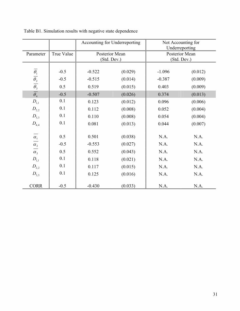
Table B1. Simulation results with negative state dependence

Accounting for Underreporting Not Accounting for Underreporting

Parameter True Value Posterior Mean (Std. Dev.)

Posterior Mean (Std. Dev.)

1θ -0.5 -0.522 (0.029) -1.096 (0.012)

2θ -0.5 -0.515 (0.014) -0.387 (0.009)

3θ 0.5 0.519 (0.015) 0.403 (0.009)

4θ -0.5 -0.507 (0.026) 0.374 (0.013)

1,1D 0.1 0.123 (0.012) 0.096 (0.006)

2,2D 0.1 0.112 (0.008) 0.052 (0.004)

3,3D 0.1 0.110 (0.008) 0.054 (0.004)

4,4D 0.1 0.081 (0.013) 0.044 (0.007) 1α 0.5 0.501 (0.038) N.A. N.A.

2α -0.5 -0.553 (0.027) N.A. N.A.

3α 0.5 0.552 (0.043) N.A. N.A.

1,1D 0.1 0.118 (0.021) N.A. N.A.

2,2D 0.1 0.117 (0.015) N.A. N.A.

3,3D 0.1 0.125 (0.016) N.A. N.A.

CORR -0.5 -0.430 (0.033) N.A. N.A.

31

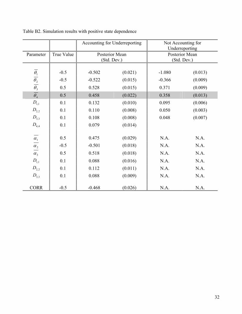
Table B2. Simulation results with positive state dependence

Accounting for Underreporting Not Accounting for Underreporting

Parameter True Value Posterior Mean (Std. Dev.)

Posterior Mean (Std. Dev.)

1θ -0.5 -0.502 (0.021) -1.080 (0.013)

2θ -0.5 -0.522 (0.015) -0.366 (0.009)

3θ 0.5 0.528 (0.015) 0.371 (0.009)

4θ 0.5 0.458 (0.022) 0.358 (0.013)

1,1D 0.1 0.132 (0.010) 0.095 (0.006)

2,2D 0.1 0.110 (0.008) 0.050 (0.003)

3,3D 0.1 0.108 (0.008) 0.048 (0.007)

4,4D 0.1 0.079 (0.014) 1α 0.5 0.475 (0.029) N.A. N.A.

2α -0.5 -0.501 (0.018) N.A. N.A.

3α 0.5 0.518 (0.018) N.A. N.A.

1,1D 0.1 0.088 (0.016) N.A. N.A.

2,2D 0.1 0.112 (0.011) N.A. N.A.

3,3D 0.1 0.088 (0.009) N.A. N.A.

CORR -0.5 -0.468 (0.026) N.A. N.A.

32

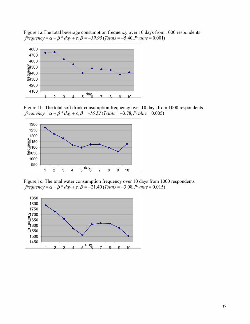
Figure 1a.The total beverage consumption frequency over 10 days from 1000 respondents )001.0,40.5(;* =−=−=++= PvalueTstats 39.95dayfrequency βεβα

41004200430044004500460047004800

1 2 3 4 5 6 7 8 9 10day

frequ

ency

Figure 1b. The total soft drink consumption frequency over 10 days from 1000 respondents

)005.0,78.3(;* =−==++= PvalueTstats -16.52dayfrequency βεβα

9501000105011001150120012501300

1 2 3 4 5 6 7 8 9 10day

frequ

ency

Figure 1c. The total water consumption frequency over 10 days from 1000 respondents

)015.0,08.3(40.21;* =−=−=++= PvalueTstats dayfrequency βεβα

145015001550160016501700175018001850

1 2 3 4 5 6 7 8 9 10day

frequ

ency

33

Table 1. Estimates on beverage consumption incidence: posterior mean (std. dev.) PROPOSED MODEL NAIVE MODEL

AGE -0.039 (0.026) 0.013 (0.012)GENDER 0.129 (0.044) -0.038 (0.028)EDUCATION 0.009 (0.019) 0.008 (0.010)INCOME 0.015 (0.013) 0.005 (0.007)LOOKGOOD 0.021 (0.024) 0.032 (0.014)INDULGE 0.709 (0.071) 0.748 (0.045)HEALTHY 0.120 (0.061) 0.199 (0.042)LOG_WEEK 0.014 (0.029) -0.036 (0.021)MEAN_MORNING 0.743 (0.122) 0.125 (0.030)MEAN_LUNCH 1.199 (0.099) 0.768 (0.031)MEAN_AFTERNOON 0.886 (0.064) 0.517 (0.027)MEAN_DINNER 1.080 (0.061) 0.864 (0.031)MEAN_NIGHT 0.231 (0.055) 0.051 (0.027)MEAN_LATE NIGHT 0.194 (0.096) -0.545 (0.037)MEAN_STATE DEPENDENCE -0.209 (0.035) -0.126 (0.021)VAR_MORNING 1.135 (0.163) 0.677 (0.046)VAR_LUNCH 0.983 (0.125) 0.624 (0.046)VAR_AFTERNOON 0.438 (0.044) 0.377 (0.031)VAR_DINNER 0.565 (0.054) 0.533 (0.041)VAR_NIGHT 0.366 (0.035) 0.433 (0.036)VAR_LATE NIGHT 1.278 (0.127) 0.959 (0.066)

CONSUMPTION

VAR_STATE DEPENDENCE 0.368 (0.034) 0.198 (0.015)AGE 0.101 (0.036) NA NAGENDER -0.287 (0.053) NA NAEDUCATION 0.007 (0.022) NA NAINCOME -0.011 (0.016) NA NALOOKGOOD 0.033 (0.027) NA NAINDULGE -0.379 (0.083) NA NAHEALTHY 0.145 (0.075) NA NADAY1 1.062 (0.139) NA NADAY2 1.007 (0.128) NA NADAY3 0.781 (0.100) NA NADAY4 0.746 (0.102) NA NADAY5 0.653 (0.094) NA NADAY6 0.707 (0.094) NA NADAY7 0.724 (0.094) NA NADAY8 0.696 (0.096) NA NADAY9 0.611 (0.089) NA NADAY10 0.746 (0.095) NA NAMORNING 0.354 (0.111) NA NALUNCH 0.851 (0.086) NA NAAFTERNOON 0.692 (0.099) NA NADINNER 1.180 (0.107) NA NANIGHT 1.041 (0.206) NA NA

REPORT

LATE NIGHT FIXED TO BE 0 NA NACORR CORR -0.838 (0.007) NA NA

Note: significant estimates at 95% are bolded in Tables 5-8.

34

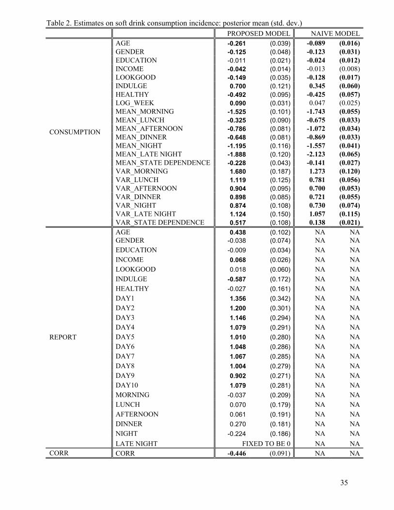
Table 2. Estimates on soft drink consumption incidence: posterior mean (std. dev.) PROPOSED MODEL NAIVE MODEL

AGE -0.261 (0.039) -0.089 (0.016)GENDER -0.125 (0.048) -0.123 (0.031)EDUCATION -0.011 (0.021) -0.024 (0.012)INCOME -0.042 (0.014) -0.013 (0.008)LOOKGOOD -0.149 (0.035) -0.128 (0.017)INDULGE 0.700 (0.121) 0.345 (0.060)HEALTHY -0.492 (0.095) -0.425 (0.057)LOG_WEEK 0.090 (0.031) 0.047 (0.025)MEAN_MORNING -1.525 (0.101) -1.743 (0.055)MEAN_LUNCH -0.325 (0.090) -0.675 (0.033)MEAN_AFTERNOON -0.786 (0.081) -1.072 (0.034)MEAN_DINNER -0.648 (0.081) -0.869 (0.033)MEAN_NIGHT -1.195 (0.116) -1.557 (0.041)MEAN_LATE NIGHT -1.888 (0.120) -2.123 (0.065)MEAN_STATE DEPENDENCE -0.228 (0.043) -0.141 (0.027)VAR_MORNING 1.680 (0.187) 1.273 (0.120)VAR_LUNCH 1.119 (0.125) 0.781 (0.056)VAR_AFTERNOON 0.904 (0.095) 0.700 (0.053)VAR_DINNER 0.898 (0.085) 0.721 (0.055)VAR_NIGHT 0.874 (0.108) 0.730 (0.074)VAR_LATE NIGHT 1.124 (0.150) 1.057 (0.115)

CONSUMPTION

VAR_STATE DEPENDENCE 0.517 (0.108) 0.138 (0.021)AGE 0.438 (0.102) NA NAGENDER -0.038 (0.074) NA NAEDUCATION -0.009 (0.034) NA NAINCOME 0.068 (0.026) NA NALOOKGOOD 0.018 (0.060) NA NAINDULGE -0.587 (0.172) NA NAHEALTHY -0.027 (0.161) NA NADAY1 1.356 (0.342) NA NADAY2 1.200 (0.301) NA NADAY3 1.146 (0.294) NA NADAY4 1.079 (0.291) NA NADAY5 1.010 (0.280) NA NADAY6 1.048 (0.286) NA NADAY7 1.067 (0.285) NA NADAY8 1.004 (0.279) NA NADAY9 0.902 (0.271) NA NADAY10 1.079 (0.281) NA NAMORNING -0.037 (0.209) NA NALUNCH 0.070 (0.179) NA NAAFTERNOON 0.061 (0.191) NA NADINNER 0.270 (0.181) NA NANIGHT -0.224 (0.186) NA NA

REPORT

LATE NIGHT FIXED TO BE 0 NA NACORR CORR -0.446 (0.091) NA NA

35

Table 3. Estimates on water consumption incidence: posterior mean (std. dev.) PROPOSED MODEL NAIVE MODEL

AGE -0.082 (0.024) -0.022 (0.015)GENDER 0.206 (0.043) 0.123 (0.028)EDUCATION 0.001 (0.016) 0.002 (0.011)INCOME -0.008 (0.010) -0.011 (0.007)GOODSEG 0.136 (0.020) 0.135 (0.016)INDULGE -0.597 (0.074) -0.653 (0.057)HEALTHY 0.809 (0.064) 0.803 (0.051)LOG_WEEK -0.052 (0.024) -0.085 (0.023)MEAN_MORNING -0.810 (0.053) -0.876 (0.036)MEAN_LUNCH -1.181 (0.041) -1.197 (0.039)MEAN_AFTERNOON -0.465 (0.047) -0.578 (0.030)MEAN_DINNER -1.183 (0.047) -1.213 (0.040)MEAN_NIGHT -0.954 (0.049) -1.025 (0.032)MEAN_LATE NIGHT -1.220 (0.064) -1.289 (0.043)MEAN_STATE DEPENDENCE -0.185 (0.025) -0.139 (0.022)VAR_MORNING 1.014 (0.086) 0.889 (0.068)VAR_LUNCH 0.896 (0.076) 0.846 (0.071)VAR_AFTERNOON 0.739 (0.060) 0.637 (0.045)VAR_DINNER 0.946 (0.075) 0.900 (0.074)VAR_NIGHT 0.651 (0.056) 0.591 (0.053)VAR_LATE NIGHT 1.190 (0.097) 1.066 (0.085)

CONSUMPTION

VAR_STATE DEPENDENCE 0.130 (0.021) 0.098 (0.015)AGE 0.634 (0.121) NA NAGENDER -0.846 (0.324) NA NAEDUCATION 0.038 (0.063) NA NAINCOME -0.013 (0.052) NA NAGOODSEG 0.078 (0.086) NA NAINDULGE -0.600 (0.291) NA NAHEALTHY 0.310 (0.270) NA NADAY1 3.060 (0.821) NA NADAY2 3.029 (0.691) NA NADAY3 2.180 (0.399) NA NADAY4 2.173 (0.405) NA NADAY5 2.006 (0.394) NA NADAY6 2.130 (0.382) NA NADAY7 2.016 (0.374) NA NADAY8 2.113 (0.382) NA NADAY9 1.945 (0.379) NA NADAY10 1.882 (0.365) NA NAMORNING -0.028 (0.280) NA NALUNCH 0.810 (0.405) NA NAAFTERNOON -0.122 (0.282) NA NADINNER 0.713 (0.420) NA NANIGHT 0.015 (0.255) NA NA

REPORT

LATE NIGHT FIXED TO BE 0 NA NACORR CORR -0.247 (0.115) NA NA

36

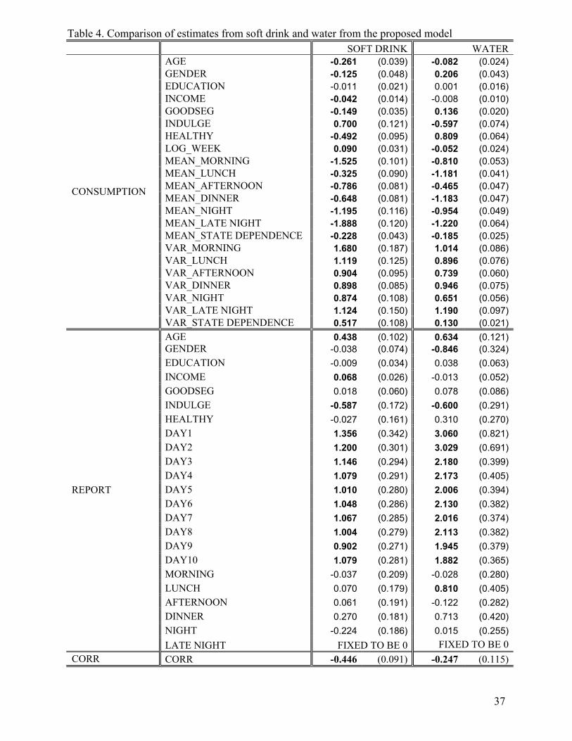
Table 4. Comparison of estimates from soft drink and water from the proposed model SOFT DRINK WATER

AGE -0.261 (0.039) -0.082 (0.024)GENDER -0.125 (0.048) 0.206 (0.043)EDUCATION -0.011 (0.021) 0.001 (0.016)INCOME -0.042 (0.014) -0.008 (0.010)GOODSEG -0.149 (0.035) 0.136 (0.020)INDULGE 0.700 (0.121) -0.597 (0.074)HEALTHY -0.492 (0.095) 0.809 (0.064)LOG_WEEK 0.090 (0.031) -0.052 (0.024)MEAN_MORNING -1.525 (0.101) -0.810 (0.053)MEAN_LUNCH -0.325 (0.090) -1.181 (0.041)MEAN_AFTERNOON -0.786 (0.081) -0.465 (0.047)MEAN_DINNER -0.648 (0.081) -1.183 (0.047)MEAN_NIGHT -1.195 (0.116) -0.954 (0.049)MEAN_LATE NIGHT -1.888 (0.120) -1.220 (0.064)MEAN_STATE DEPENDENCE -0.228 (0.043) -0.185 (0.025)VAR_MORNING 1.680 (0.187) 1.014 (0.086)VAR_LUNCH 1.119 (0.125) 0.896 (0.076)VAR_AFTERNOON 0.904 (0.095) 0.739 (0.060)VAR_DINNER 0.898 (0.085) 0.946 (0.075)VAR_NIGHT 0.874 (0.108) 0.651 (0.056)VAR_LATE NIGHT 1.124 (0.150) 1.190 (0.097)

CONSUMPTION

VAR_STATE DEPENDENCE 0.517 (0.108) 0.130 (0.021)AGE 0.438 (0.102) 0.634 (0.121)GENDER -0.038 (0.074) -0.846 (0.324)EDUCATION -0.009 (0.034) 0.038 (0.063)INCOME 0.068 (0.026) -0.013 (0.052)GOODSEG 0.018 (0.060) 0.078 (0.086)INDULGE -0.587 (0.172) -0.600 (0.291)HEALTHY -0.027 (0.161) 0.310 (0.270)DAY1 1.356 (0.342) 3.060 (0.821)DAY2 1.200 (0.301) 3.029 (0.691)DAY3 1.146 (0.294) 2.180 (0.399)DAY4 1.079 (0.291) 2.173 (0.405)DAY5 1.010 (0.280) 2.006 (0.394)DAY6 1.048 (0.286) 2.130 (0.382)DAY7 1.067 (0.285) 2.016 (0.374)DAY8 1.004 (0.279) 2.113 (0.382)DAY9 0.902 (0.271) 1.945 (0.379)DAY10 1.079 (0.281) 1.882 (0.365)MORNING -0.037 (0.209) -0.028 (0.280)LUNCH 0.070 (0.179) 0.810 (0.405)AFTERNOON 0.061 (0.191) -0.122 (0.282)DINNER 0.270 (0.181) 0.713 (0.420)NIGHT -0.224 (0.186) 0.015 (0.255)

REPORT

LATE NIGHT FIXED TO BE 0 FIXED TO BE 0CORR CORR -0.446 (0.091) -0.247 (0.115)

37

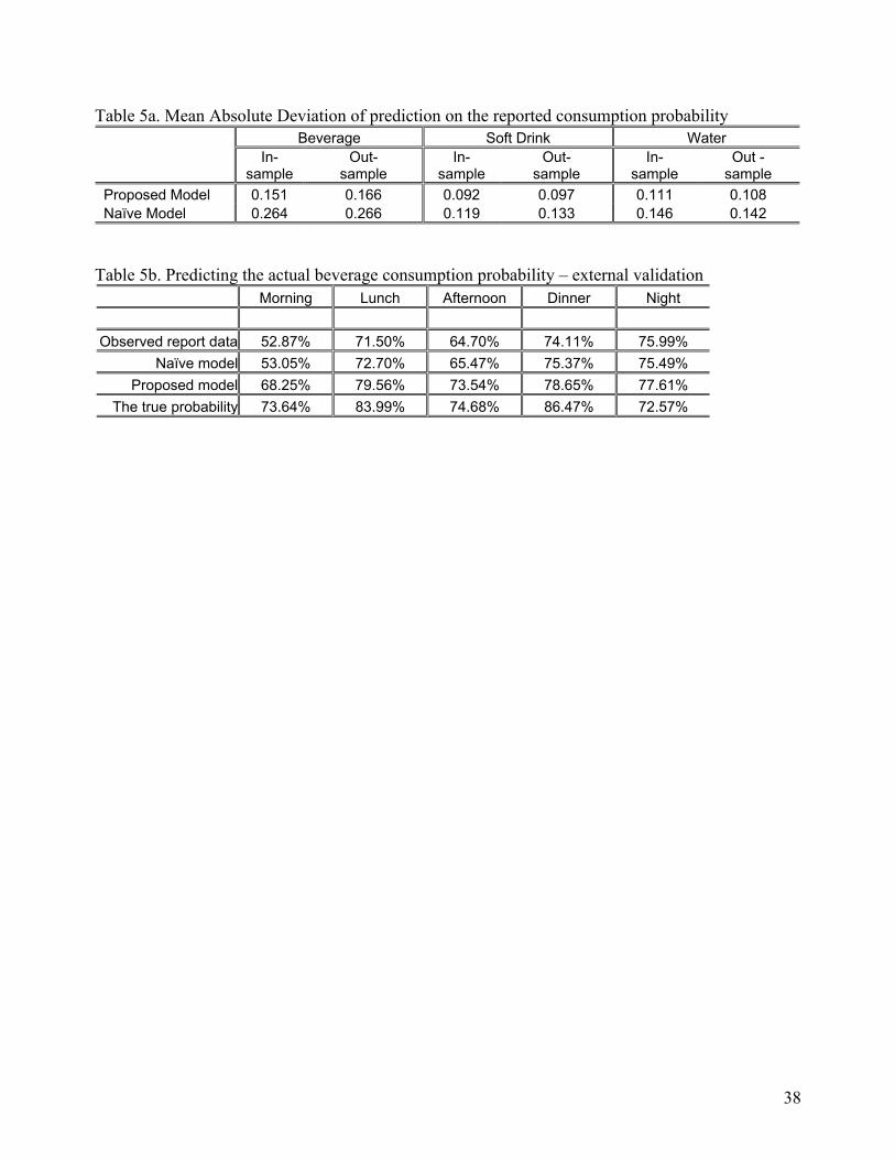
Table 5a. Mean Absolute Deviation of prediction on the reported consumption probability Beverage Soft Drink Water

In-

sample Out-

sample In-

sample Out-

sample In-

sample Out -

sample Proposed Model 0.151 0.166 0.092 0.097 0.111 0.108 Naïve Model 0.264 0.266 0.119 0.133 0.146 0.142

Table 5b. Predicting the actual beverage consumption probability – external validation

Morning Lunch Afternoon Dinner Night

Observed report data 52.87% 71.50% 64.70% 74.11% 75.99% Naïve model 53.05% 72.70% 65.47% 75.37% 75.49%

Proposed model 68.25% 79.56% 73.54% 78.65% 77.61% The true probability 73.64% 83.99% 74.68% 86.47% 72.57%

38

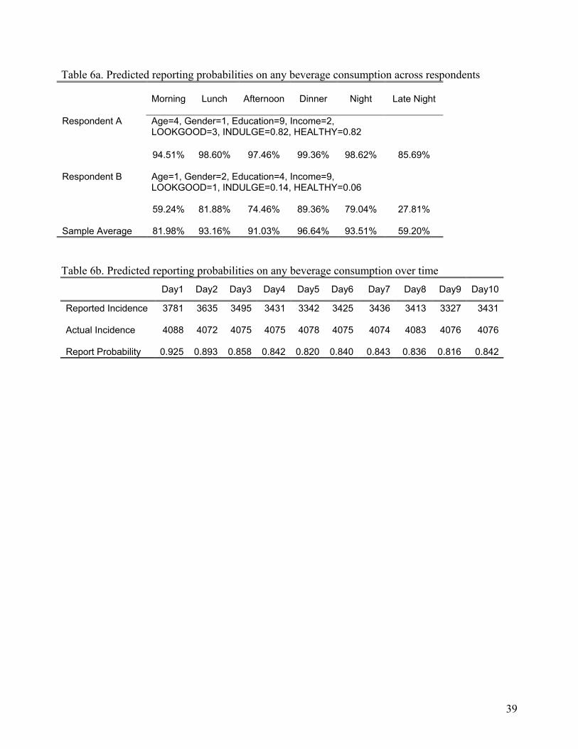
Table 6a. Predicted reporting probabilities on any beverage consumption across respondents

Morning Lunch Afternoon Dinner Night

Late Night

Respondent A Age=4, Gender=1, Education=9, Income=2, LOOKGOOD=3, INDULGE=0.82, HEALTHY=0.82

94.51% 98.60% 97.46% 99.36% 98.62% 85.69% Respondent B

Age=1, Gender=2, Education=4, Income=9, LOOKGOOD=1, INDULGE=0.14, HEALTHY=0.06

59.24% 81.88% 74.46% 89.36% 79.04% 27.81% Sample Average 81.98% 93.16% 91.03% 96.64% 93.51% 59.20% Table 6b. Predicted reporting probabilities on any beverage consumption over time Day1 Day2 Day3 Day4 Day5 Day6 Day7 Day8 Day9 Day10

Reported Incidence 3781 3635 3495 3431 3342 3425 3436 3413 3327 3431 Actual Incidence 4088 4072 4075 4075 4078 4075 4074 4083 4076 4076 Report Probability 0.925 0.893 0.858 0.842 0.820 0.840 0.843 0.836 0.816 0.842

39

References Bailar, Barbara A. (1975), “The Effects of Rotation Group Bias on Estimates from Panel Surveys,” Journal of the American Statistical Association, 70 (March), 23-30. Baumgartner, Hans and Jan-Benedict E.M. Steenkamp (2001), “Response Styles in Marketing Research: A Cross-National Investigation, ” Journal of Marketing Research, 38 (2), 143-156. Bollinger, Christopher R. and Martin H. David (1997), “Modeling Discrete Choice with Response Error: Food Stamp Participation,” Journal of the American Statistical Association, 92, 827-835. Bradlow, Eric T. and Alan M. Zaslavsky (1999), “A Hierarchical Latent Variable Model for Ordinal Data from a Customer Satisfaction Survey with "No Answer" Responses,” Journal of the American Statistical Association, Vol. 94, No. 445. Mar., pp. 43-52. Bradlow, Eric, Ye Hu, and Teck Ho (2004a), "A Learning-Based Model for Imputing Missing Levels in Partial Conjoint Profiles," Journal of Marketing Research, 41(4), 369-381. Che, Hai, K. Sudhir, and P.B. Seetharaman (2007), "Bounded Rationality in Pricing under State Dependent Demand: Do Firms Look Ahead? How Far Ahead?" Journal of Marketing Research, 44 (3), 434-449. De Jong, Martijn G., Jan Benedict E.M. Steenkamp, Jean-Paul Fox, and Hans Baumgarter (2008), " Using Item Response Theory to Measure Extreme Response Style in Marketing Research: A Global Investigation," Journal of Marketing Research, 45 (1), 104-115. Du, Rex and Wagner Kamakura (2006), “Household Life Cycles and Lifestyles in the United States," Journal of Marketing Research, 43 (1), 121-132. Erdem, Tülin and Michael P. Keane (1996), “Decision-Making under Uncertainty: Capturing Dynamic Choice Processes in Turbulent Consumer Goods Markets,” Marketing Science, 15 (1), 1-20. Fisher, Robert J. (1993). “Social Desirability Bias and the Validity of Indirect Questioning,” Journal of Consumer Research, 20 (3), 303–315. Fuller, Wayne A. (1995), “Estimation in the Presence of Measurement Error,” International Statistical Review, 63(2), 121-141. Ganster, D. C., H. W. Hennessey, and F. Luthans (1983), “Social Desirability Response Effects: Three Alternative Models.” Academy of Management Journal, 26 (2), 321–331. Geweke, J. (1992), “Evaluating the accuracy of sampling-based approaches to the calculation of posterior moments,” Bayesian Statistics 4. Oxford University Press, Oxford, 169–193.

40

De Jong, Martijn G., Rik Pieters, and Jean-Paul Fox (2009), “Reducing Social Desirability Bias Via Item Randomized Response: An Application to Measure Underreported Desires,” Journal of Marketing Research, forthcoming. Gilbride, Tim, Sha Yang and Greg M. Allenby (2005), "Modeling Simultaneity in Survey Data," Quantitative Marketing and Economics, 3, 311-315 Guadagni, Peter M. and John D. C. Little (1983) "A Logit Model of Brand Choice Calibrated on Scanner Data" Marketing Science, 2, 3, 203-238. Hawkins, Del I. and Kenneth A. Coney (1981), “Uninformed Response Error in Survey Research,” Journal of Marketing Research, 18 (August), 370-374. Kitamura, Ryuichi and Piet H. L. Bovy (1987), “Analysis of Attribution Biases and Trip Reporting Errors for Panel Data,” Transportation Research A, 21A (4/5), 287-302. Lee Eunkyu, Michael Y. Hu and Rex S. Toh (2000), “Are Consumer Survey Results Distorted? Systematic Impact of Behavioral Frequency and Duration on Survey Response Errors,” Journal of Marketing Research, 37 (February), 125-133. Liechty, John C., Duncan K.H. Fong, and Wayne DeSarbo (2005), “Dynamic Models with Individual Level Heterogeneity: Applied to Evolution During Conjoint Studies,” Marketing Science, 24 (2), 285-293. Mandell, Lewis and Lorman L. Lundsten (1978), “Some Insights into the Underreporting of Financial Data by Sample Survey Respondents,” Journal of Marketing Research, 15 (May), 294-299. Menon, Geeta (1993), “The Effects of Accessibility of Information in Memory on Judgments of Behavioral Frequencies,” Journal of Consumer Research, 20 (December), 431-440. Menon, Geeta (1995), “Are the Parts Better Than the Whole? The Effects of Decompositional Questions on Judgments of Frequency Behaviors,” Journal of Marketing Research, 34 (August), 335-346. Myung-soo Jo, James Nelson and Pamela Kiecker (1997), “A Model for Controlling Social Desirability Bias by Direct and Indirect Questioning,” Marketing Letters, 8 (4), 429-437 Montgomery, Alan L., Shibo Li, Kannan Srinivasan, and John C. Liechty (2004), “Modeling Online Browsing and Path Analysis Using Clickstream Data,” Marketing Science, 23 (4), 579-595. Montoya, Ricardo, Oded Netzer and Kamel Jedidi (2007), “Dynamic Marketing Mix Allocation for Long-Term Profitability,” Working Paper, Columbia University. Netzer, Oded, James Lattin, and V. Srinivasan 2008), “A Hidden Markov Model of Customer Relationship Dynamics,” Marketing Science, 27 (2), 185–204.

41

42

Otter, Thomas, Sylvia Frühwirth-Schnatter and Regina Tüchler (2003), "Unobserved Preference Changes in Conjoint Analysis", Working Paper, Fisher College of Business, Ohio State University. Rossi, Peter E., Zvi Gilula and Greg M. Allenby (2001), “Overcoming Scale Usage Heterogeneity: A Bayesian Hierarchical Approach,” Journal of the American Statistical Association, 96 (1), 20-31. Seetharaman, P. B., A.K. Ainslie, and P.K. Chintagunta (1999). "Investigating Household State Dependence Effects Across Categories," Journal of Marketing Research, 36 (4), 488-500 Sudman, Seymour (1964), “On the Accuracy of Recording of Consumer Panels: Impact of some demographic factors and behavioral characteristics on systematic attrition”, Journal of Marketing Research, 1 (May), 14-20. Ter Hofstede, Frenkel, Jan-Benedict E.M. Steenkamp, and Michel Wedel (1999), “International Market Segmentation Based on Consumer-Product Relations,” Journal of Marketing Research, 36 (February), 1-17. Toh, Rex S. and Michael Y. Hu (1996), “Natural mortality and participation fatigue as potential biases in diary panels: Impact of some demographic factors and behavioral characteristics on systematic attrition,” Journal of Business Research, 35(2), 129-138. Turner, R. (1961), “Inter-Week Variations in Expenditure Recorded During a Two-Week Survey of Family Expenditure,” Applied Statistics, 10(3), 136-146. van der Lans, Ralf, Gerrit van Bruggen, Jehoshua Eliashberg and Berend Wierenga, “A Viral Branding Model for Predicting the Spread of Electronic Word-of-Mouth,” Marketing Science, Forthcoming. Waksberg, J. and J. Neter (1965), “Response Errors in Collection of Expenditures Data by Household Interviews: An Experimental Study,” Technical Paper No. 11, U.S. Bureau of the Census, Washington, D.C.: U.S. Government Printing Office.