Embed Size (px)
Citation preview

DISC School - April 2003
Modeling, Control, and ReachabilityAnalysis of Discrete-Time Hybrid Systems
Alberto Bemporad
Dept. of Information Engineering
University of Siena, Italy
http://www.dii.unisi.it/~bemporad
March 30, 2003
2
Abstract
These notes describe a computational framework for modeling, controlling, and analyz-ing hybrid systems in discrete-time. We describe three classes of hybrid models in detail:discrete hybrid automata (DHA), piecewise affine (PWA) systems, and mixed logical dy-namical (MLD) systems. We show the relations among such model classes and otherexisting model paradigms, such as (extended) linear complementarity ((E)LC) systemsand min-max-plus-scaling (MMPS) systems. We present the language HYSDEL (HYbridSystems DEscription Language), a high level modeling language for describing discrete-time hybrid systems, and a set of tools for translating DHA into any of the former hybridmodels.
We describe controller synthesis strategies based on the receding horizon solution tofinite-time optimal control problems via mixed-integer programming and via multipara-metric programming, by extending to hybrid systems ideas and results that exist forModel Predictive Control (MPC) of linear systems.
We also present a methodology for computing the set of states that a discrete-timeaffine hybrid system can reach by starting from a given set of initial conditions andunder the effect of exogenous inputs to the system, such as disturbances, within aprescribed range. We show how to use reachability analysis to assess robust stability,safety, and liveness properties of the hybrid system, and how the reach-set computa-tion machinery can be embedded in an optimization procedure to determine solve quitegeneral hybrid optimal control problems.
Finally, we present a complete automotive case study showing the modeling capa-bilities of HYSDEL and how the different models allow to use several computationaltools.
c©2003 by A. Bemporad, University of Siena
All rights reserved. No part of the publication may be reproduced in any form by print,photoprint, microfilm or any other means without written permission from the author.
Contents
1 Introduction 5
2 Modeling 112.1 Piecewise Affine (PWA) Systems . . . . . . . . . . . . . . . . . . . . . . . . . . 112.2 Discrete Hybrid Automata . . . . . . . . . . . . . . . . . . . . . . . . . . . . . 12
2.2.1 Switched Affine System (SAS) . . . . . . . . . . . . . . . . . . . . . . . 132.2.2 Event Generator (EG) . . . . . . . . . . . . . . . . . . . . . . . . . . . . 132.2.3 Finite State Machine (FSM ) . . . . . . . . . . . . . . . . . . . . . . . . . 132.2.4 Mode Selector (MS) . . . . . . . . . . . . . . . . . . . . . . . . . . . . . . 152.2.5 DHA Trajectories . . . . . . . . . . . . . . . . . . . . . . . . . . . . . . . 15
2.3 Discrete Hybrid Automata and Piecewise Affine Systems . . . . . . . . . . . 162.4 Logic and Mixed-Integer Inequalities . . . . . . . . . . . . . . . . . . . . . . . 16
2.4.1 Logical Functions . . . . . . . . . . . . . . . . . . . . . . . . . . . . . . 162.4.2 Continuous-Logic Interfaces . . . . . . . . . . . . . . . . . . . . . . . . 18
2.5 Mixed Logical Dynamical Systems . . . . . . . . . . . . . . . . . . . . . . . . . 182.6 Other Computational Models and Further Equivalences . . . . . . . . . . . . 20
2.6.1 Linear Complementarity Systems . . . . . . . . . . . . . . . . . . . . . 202.6.2 Extended Linear Complementarity (ELC) Systems . . . . . . . . . . . . 212.6.3 Max-Min-Plus-Scaling (MMPS) Systems . . . . . . . . . . . . . . . . . 212.6.4 Equivalence Results . . . . . . . . . . . . . . . . . . . . . . . . . . . . . 22
2.7 HYSDEL Models . . . . . . . . . . . . . . . . . . . . . . . . . . . . . . . . . . . 232.8 A Simple Example . . . . . . . . . . . . . . . . . . . . . . . . . . . . . . . . . . 252.9 Identification of Hybrid Systems . . . . . . . . . . . . . . . . . . . . . . . . . . 26
3 Controller Synthesis 273.1 Introduction . . . . . . . . . . . . . . . . . . . . . . . . . . . . . . . . . . . . . 273.2 Model Predictive Control for Hybrid Systems . . . . . . . . . . . . . . . . . . 28
3.2.1 Closed-Loop Stability . . . . . . . . . . . . . . . . . . . . . . . . . . . . 293.2.2 MPC Optimization Problem . . . . . . . . . . . . . . . . . . . . . . . . . 313.2.3 MILP Associated with MPC . . . . . . . . . . . . . . . . . . . . . . . . . 313.2.4 Mixed Integer Program Solvers . . . . . . . . . . . . . . . . . . . . . . . 32
3.3 Explicit Hybrid MPC Control Laws . . . . . . . . . . . . . . . . . . . . . . . . 333.3.1 Multiparametric-MILP Solvers . . . . . . . . . . . . . . . . . . . . . . . 34
4 Reachability Analysis 394.1 Preliminaries on Polyhedral Computation . . . . . . . . . . . . . . . . . . . . 404.2 Reach-Set Computation . . . . . . . . . . . . . . . . . . . . . . . . . . . . . . . 42
4.2.1 Switching Sequences . . . . . . . . . . . . . . . . . . . . . . . . . . . . 424.2.2 Determination of the Reachable Set . . . . . . . . . . . . . . . . . . . . 43
4.3 Approximate Reachability Analysis . . . . . . . . . . . . . . . . . . . . . . . . 464.3.1 Approximation of Intersections . . . . . . . . . . . . . . . . . . . . . . . 46
4.4 Verification of Safety Properties . . . . . . . . . . . . . . . . . . . . . . . . . . 484.4.1 Applications . . . . . . . . . . . . . . . . . . . . . . . . . . . . . . . . . . 50
3

4 CONTENTS
4.5 Performance Assessment of Hybrid MPC . . . . . . . . . . . . . . . . . . . . . 504.6 Optimal Control Solutions Based on Reachability Analysis . . . . . . . . . . 53
4.6.1 Variations to the Optimization Algorithm . . . . . . . . . . . . . . . . . 574.7 Conclusions . . . . . . . . . . . . . . . . . . . . . . . . . . . . . . . . . . . . . . 59
5 Application Examples 615.1 Analysis and Control of a Cruise Control System . . . . . . . . . . . . . . . . 61
5.1.1 Car model . . . . . . . . . . . . . . . . . . . . . . . . . . . . . . . . . . . 615.1.2 Reachability Analysis . . . . . . . . . . . . . . . . . . . . . . . . . . . . 635.1.3 Cruise Control Design . . . . . . . . . . . . . . . . . . . . . . . . . . . . 65
6 Conclusions 71
Chapter 1
Introduction
The mathematical model of a system is traditionally associated with differential or dif-ference equations, typically derived from physical laws governing the dynamics of thesystem under consideration. Consequently, most of the control theory and tools havebeen developed for such systems, in particular for systems whose evolution is describedby smooth linear or nonlinear state transition functions. On the other hand, in manyapplications the system to be controlled is also constituted by parts described by logic,such as for instance on/off switches or valves, gears or speed selectors, and evolutionsdependent on if-then-else rules. Often, the control of these systems is left to schemesbased on heuristic rules inferred from practical plant operation.
Recent technological innovations have caused a considerable interest in the study ofdynamical processes of a heterogeneous continuous and discrete nature, denoted as hy-brid systems. The peculiarity of hybrid systems is the interaction between continuous-time dynamics (governed by differential or difference equations), and discrete dynamicsand logic rules (described by temporal logic, finite state machines, if-then-else condi-tions, discrete events, etc.) and discrete components (on/off switches, selectors, digitalcircuitry, software code, etc.).
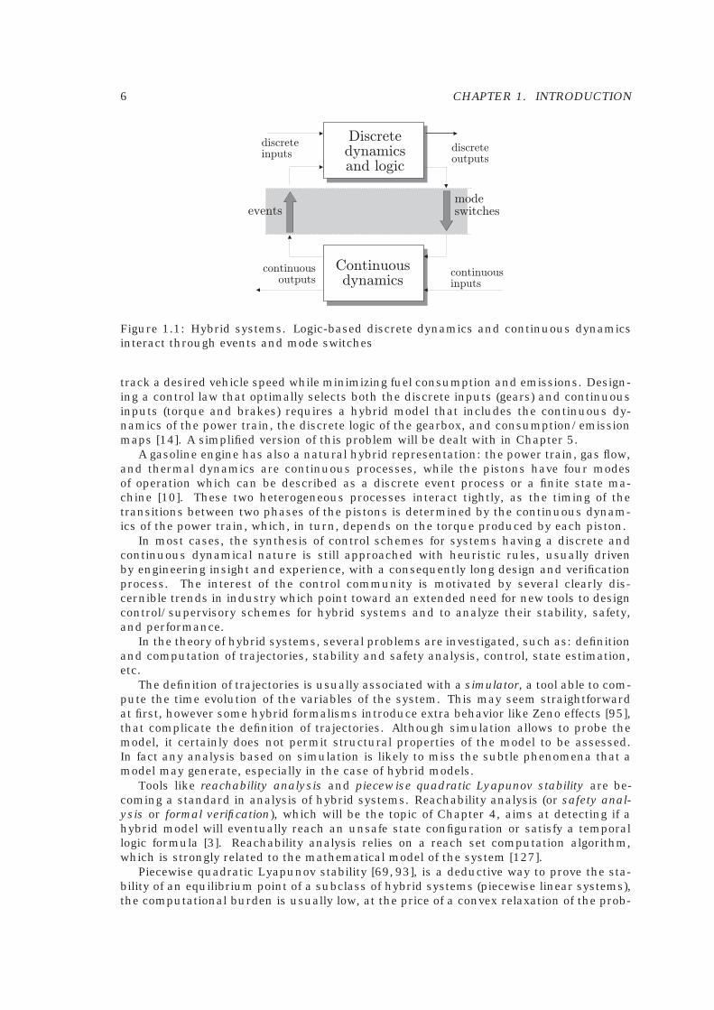
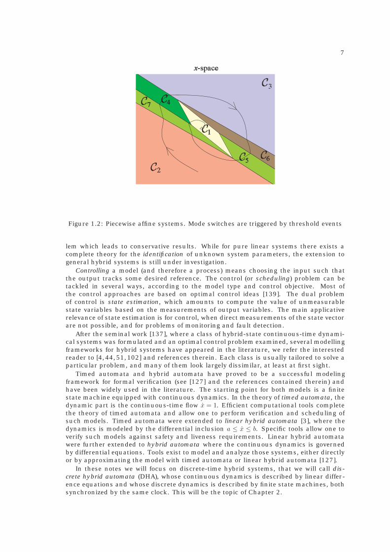
Hybrid systems switch among many operating modes, where each mode is governedby its own characteristic dynamical laws. Mode transitions are triggered by variablescrossing specific thresholds (state events), by the elapse of certain time periods (timeevents), or by external inputs (input events) [4]. A typical example of hybrid systems areembedded systems, constituted by dynamical components governed by logical/discretedecision components. Complex systems organized in hierachical way, where for in-stance discrete planning algorithms at the higher level interact with continuous con-trol algorithms and processes at the lower level, are another example of hybrid sys-tems. In these systems, a hierarchical organization helps managing the complexity ofthe system, as higher levels in the hierarchy require less detailed models (=abstrac-tions) of the functioning of the lower levels. Two main categories of hybrid systemswere successfully adopted for analysis and synthesis purposes [44]: hybrid control sys-tems [3,5,31,101,103], which consist of the interaction between continuous dynamicalsystems and discrete/logic automata (Fig. 1.1), and switched systems [45,93,128,138],where the state-space is partitioned into regions, each one being associated with a dif-ferent continuous dynamics (Fig. 1.2).
Hybrid systems arise in a large number of application areas and are attracting in-creasing attention in both academic theory-oriented circles as well as in industry, forinstance the automotive industry [9,10,14,23,94]. Moreover, many physical phenomenaadmit a natural hybrid description, like circuits integrating relays or diodes, biomolec-ular networks [2], and TCP/IP networks in [90].
As an example of hybrid control problem consider the design of a cruise control sys-tem that commands the gear shift, the engine torque, and the braking force in order to
5
6 CHAPTER 1. INTRODUCTION
Discretedynamicsand logic
Continuousdynamics
continuousoutputs
discreteinputs
discreteoutputs
continuousinputs
eventsmodeswitches
Figure 1.1: Hybrid systems. Logic-based discrete dynamics and continuous dynamicsinteract through events and mode switches
track a desired vehicle speed while minimizing fuel consumption and emissions. Design-ing a control law that optimally selects both the discrete inputs (gears) and continuousinputs (torque and brakes) requires a hybrid model that includes the continuous dy-namics of the power train, the discrete logic of the gearbox, and consumption/emissionmaps [14]. A simplified version of this problem will be dealt with in Chapter 5.
A gasoline engine has also a natural hybrid representation: the power train, gas flow,and thermal dynamics are continuous processes, while the pistons have four modesof operation which can be described as a discrete event process or a finite state ma-chine [10]. These two heterogeneous processes interact tightly, as the timing of thetransitions between two phases of the pistons is determined by the continuous dynam-ics of the power train, which, in turn, depends on the torque produced by each piston.
In most cases, the synthesis of control schemes for systems having a discrete andcontinuous dynamical nature is still approached with heuristic rules, usually drivenby engineering insight and experience, with a consequently long design and verificationprocess. The interest of the control community is motivated by several clearly dis-cernible trends in industry which point toward an extended need for new tools to designcontrol/supervisory schemes for hybrid systems and to analyze their stability, safety,and performance.
In the theory of hybrid systems, several problems are investigated, such as: definitionand computation of trajectories, stability and safety analysis, control, state estimation,etc.
The definition of trajectories is usually associated with a simulator, a tool able to com-pute the time evolution of the variables of the system. This may seem straightforwardat first, however some hybrid formalisms introduce extra behavior like Zeno effects [95],that complicate the definition of trajectories. Although simulation allows to probe themodel, it certainly does not permit structural properties of the model to be assessed.In fact any analysis based on simulation is likely to miss the subtle phenomena that amodel may generate, especially in the case of hybrid models.
Tools like reachability analysis and piecewise quadratic Lyapunov stability are be-coming a standard in analysis of hybrid systems. Reachability analysis (or safety anal-ysis or formal verification), which will be the topic of Chapter 4, aims at detecting if ahybrid model will eventually reach an unsafe state configuration or satisfy a temporallogic formula [3]. Reachability analysis relies on a reach set computation algorithm,which is strongly related to the mathematical model of the system [127].
Piecewise quadratic Lyapunov stability [69, 93], is a deductive way to prove the sta-bility of an equilibrium point of a subclass of hybrid systems (piecewise linear systems),the computational burden is usually low, at the price of a convex relaxation of the prob-
7
Figure 1.2: Piecewise affine systems. Mode switches are triggered by threshold events
lem which leads to conservative results. While for pure linear systems there exists acomplete theory for the identification of unknown system parameters, the extension togeneral hybrid systems is still under investigation.
Controlling a model (and therefore a process) means choosing the input such thatthe output tracks some desired reference. The control (or scheduling) problem can betackled in several ways, according to the model type and control objective. Most ofthe control approaches are based on optimal control ideas [139]. The dual problemof control is state estimation, which amounts to compute the value of unmeasurablestate variables based on the measurements of output variables. The main applicativerelevance of state estimation is for control, when direct measurements of the state vectorare not possible, and for problems of monitoring and fault detection.
After the seminal work [137], where a class of hybrid-state continuous-time dynami-cal systems was formulated and an optimal control problem examined, several modellingframeworks for hybrid systems have appeared in the literature, we refer the interestedreader to [4,44,51,102] and references therein. Each class is usually tailored to solve aparticular problem, and many of them look largely dissimilar, at least at first sight.
Timed automata and hybrid automata have proved to be a successful modelingframework for formal verification (see [127] and the references contained therein) andhave been widely used in the literature. The starting point for both models is a finitestate machine equipped with continuous dynamics. In the theory of timed automata, thedynamic part is the continuous-time flow x = 1. Efficient computational tools completethe theory of timed automata and allow one to perform verification and scheduling ofsuch models. Timed automata were extended to linear hybrid automata [3], where thedynamics is modeled by the differential inclusion a ≤ x ≤ b. Specific tools allow one toverify such models against safety and liveness requirements. Linear hybrid automatawere further extended to hybrid automata where the continuous dynamics is governedby differential equations. Tools exist to model and analyze those systems, either directlyor by approximating the model with timed automata or linear hybrid automata [127].
In these notes we will focus on discrete-time hybrid systems, that we will call dis-crete hybrid automata (DHA), whose continuous dynamics is described by linear differ-ence equations and whose discrete dynamics is described by finite state machines, bothsynchronized by the same clock. This will be the topic of Chapter 2.
8 CHAPTER 1. INTRODUCTION
A particular case of DHA is the popular class of piecewise affine (PWA) systems firstintroduced by Sontag [128]. Essentially, PWA are switched affine systems whose modeonly depends on the current location of the state vector. More precisely, the state spaceis partitioned into polyhedral regions, as depicted in Figure 1.2, and each region isassociated with a different affine state-update equation (more generally, the partitionis defined in the combined space of state and input vectors). We will actually showthat DHA and PWA systems are equivalent model classes, and hence, in particular, thatgeneric DHA systems can be converted to equivalent PWA systems.
Another popular class of hybrid systems is the class of linear complementarity (LC)systems [53,87,88,126,134]. LC systems were mainly investigated in continuous-time,and applications include constrained mechanical systems, electrical networks with idealdiodes or other dynamical systems with piecewise linear relations, variable structuresystems, constrained optimal control problems, projected dynamical systems and soon [87, Ch. 2]. Issues related to modeling, well-posedness (existence and uniqueness ofsolution trajectories), simulation and discretization have been of particular interest.
In Chapter 2 we will show that DHA models are a mathematical abstraction of thefeatures provided by other computational oriented and domain specific hybrid frame-works: Mixed logical dynamical (MLD) models [31], the aforementioned piecewise affine(PWA) systems [128] and linear complementarity (LC), extended linear complementarity(ELC) systems [62, 63], and max-min-plus-scaling (MMPS) systems [65]. In particular,as shown in [86] all those modeling frameworks are equivalent (possibly under somehypothesis) and it is possible to represent the same system with models of each class.
As we already mentioned, we will work with discrete-time hybrid models. Despite thefact that the effects of sampling can be neglected in most applications, we note, however,that interesting mathematical phenomena occurring in hybrid systems, such as Zenobehaviors [95] do not exist in discrete-time. On the other hand, most of these phenom-ena are usually a consequence of the continuous-time switching model, rather than thereal natural behavior. Our main motivation for concentrating on discrete-time modelsstems from the need to analyze these systems and to solve optimization problems, suchas optimal control or scheduling problems, for which the continuous-time counterpartwould not be easily computable. Although it is possible to consider hybrid automatain continuous-time, several computational tools profit from the discretization of time1.As anticipated DHA generalize many computational oriented models for hybrid systemsand therefore represent the starting point for solving complex analysis and synthesisproblems for hybrid systems.
In particular the MLD and PWA frameworks allow one to recast reachability/observabilityanalysis, optimal control, and estimation as mathematical programming problems. Reach-ability analysis algorithms were developed in [37] for stability and performance analysisof hybrid PWA systems. In [25, 132] the authors also presented a novel approach forsolving scheduling problems using combined reachability analysis and quadratic opti-mization for MLD and PWA models. For feedback control, in [31] the authors propose amodel predictive control scheme which is able to stabilize MLD systems on desired ref-erence trajectories while fulfilling operating constraints, and possibly take into accountprevious qualitative knowledge in the form of heuristic rules. This will be the topic ofChapter 3. Similarly, the dual problem of state estimation admits a receding horizonsolution scheme [30,71,107].
Several authors focused on the problem of solving optimal control problems for hy-brid systems. For continuous-time hybrid systems, most of the literature either studiednecessary conditions for a trajectory to be optimal [116, 129], or focused on the com-putation of optimal/suboptimal solutions by means of dynamic programming or themaximum principle [46,47,82,85,100,121,138,139].
The hybrid optimal control problem becomes less complex when the dynamics is
1Also some tools for continuous-time hybrid models perform internally a time discretization of the modelin order to execute the computations [127].
9
HYSDEL Model
MLD + PWA Model
Reachability Analysis
Process
Controller Design Stability Analysis
Filter Design
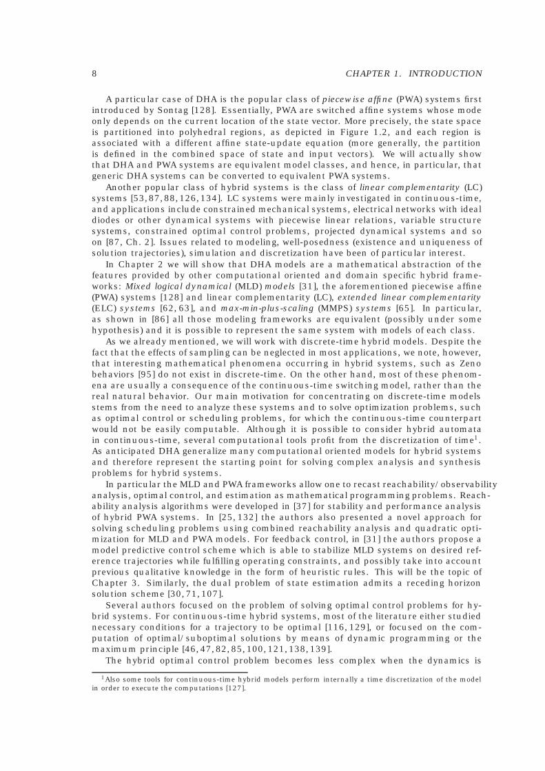
Figure 1.3: Design flow: The process is modeled in HYSDEL. The model is automaticallytranslated into MLD and PWA form, and used for analysis/synthesis
expressed in discrete-time, as the main source of complexity becomes the combinato-rial (yet finite) number of possible switching sequences. In particular, in [16, 31, 131]the authors have solved optimal control problems for discrete-time hybrid systems bytransforming the hybrid model into a set of linear equalities and inequalities involvingboth real and (0-1) variables, so that the optimal control problem can be solved by amixed-integer programming (MIP) solver.
In these notes we will refer to the tool HYSDEL (HYbrid Systems DEscription Lan-guage), a high level language for modeling and simulating DHA, and for automaticallytranslating DHA into MLD and PWA models. The idea is to model hybrid systems asDHA using HYSDEL, then use MLD and PWA models as a computationally convenientmodel — defined by a collection of equalities and inequalities and therefore often hardto determine by hand – for analysis and synthesis purposes. The idea is depicted inFigure 1.3/
Finally, we mention that identification techniques for piecewise affine systems wererecently developed [20, 34, 72, 97], that allow one to derive models (or parts of models)from input/output data.

10 CHAPTER 1. INTRODUCTION
Chapter 2
Modeling
In this chapter we introduce the basic discrete time hybrid models considered in thisnotes: piecewise affine (PWA) models, mixed logical dynamical (MLD) models, and dis-crete hybrid automata (DHA).
After introducing PWA systems, we will go through the steps needed for modeling asystem as a DHA. We will first detail the process of translating propositional logic in-volving Boolean variables and linear threshold events over continuous variables intomixed-integer linear inequalities, generalizing several results available in the litera-ture [31, 119, 136], in order to get an equivalent MLD form of a DHA system. We willalso recall the key equivalence results among several classes of discrete-time hybridsystems, so that existing analysis and synthesis tools developed for a particular classcan be easily transferred to the other classes.
We will present the tool HYSDEL (=HYbrid Systems DEscription Language), that al-lows describing the hybrid dynamics in a textual form, and a related compiler whichprovides different model representations of the given hybrid dynamics. The HYSDELcompiler is available at http://control.ee.ethz.ch/~hybrid/hysdel.
A complete automotive case study is reported in Chapter 5, where we will derivea model of the car engine and power train, and, using that model, solve a controllersynthesis and a safety analysis problem.
2.1 Piecewise Affine (PWA) Systems
PWA systems [86, 128] are defined by partitioning the space of states and inputs intopolyhedral regions (cf. Figure 1.2) and associating with each region a different linearstate-update equation
x′(k) = Ai(k)x(k) +Bi(k)u(k) + fi(k) (2.1a)
y(k) = Ci(k)x(k) +Di(k)u(k) + gi(k) (2.1b)
i(k) such that
Hi(k)x(k) + Ji(k)u(k) ≤ Ki(k), (2.1c)
Hi(k)x(k) + Ji(k)u(k) < Ki(k), (2.1d)
where x ∈ X ⊆ Rn, u ∈ U ⊆ R
m, y ∈ Y ⊆ Rp, the matrices Ai(k), Bi(k), fi(k), Ci(k), Di(k),
gi(k), Hi(k), Ji(k), Ki(k), Hi(k), Ji(k), Ki(k) are constant and have suitable dimensions, x′(k)denotes the successor x(k + 1) of x(k), i(k) ∈ Is � {1, . . . , s}, the inequalities in (2.1c) and(2.1d) should be interpreted component-wise and the constraints (2.1c) and (2.1d) definea polyhedral partition {Pi}i=1,...,s of the set X × U . In the sequel, we denote by Xi(k) thesubset of X ×U defined by (2.1c)–(2.1d). When only numerical aspects are of interest, wecan consider all the inequalities in (2.1c)–(2.1d) to be non strict, as discussed in [131].
11
12 CHAPTER 2. MODELING
xr(k)
ur(k)
i(k)
i(k − 1)
xb(k)
ub(k)
δe(k)
SAS
Automaton (EG) EventGenerator
(MS) ModeSelector
Clock
z−1
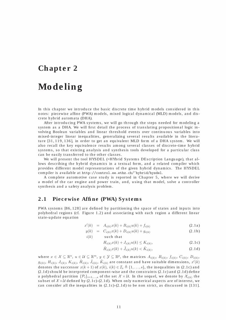
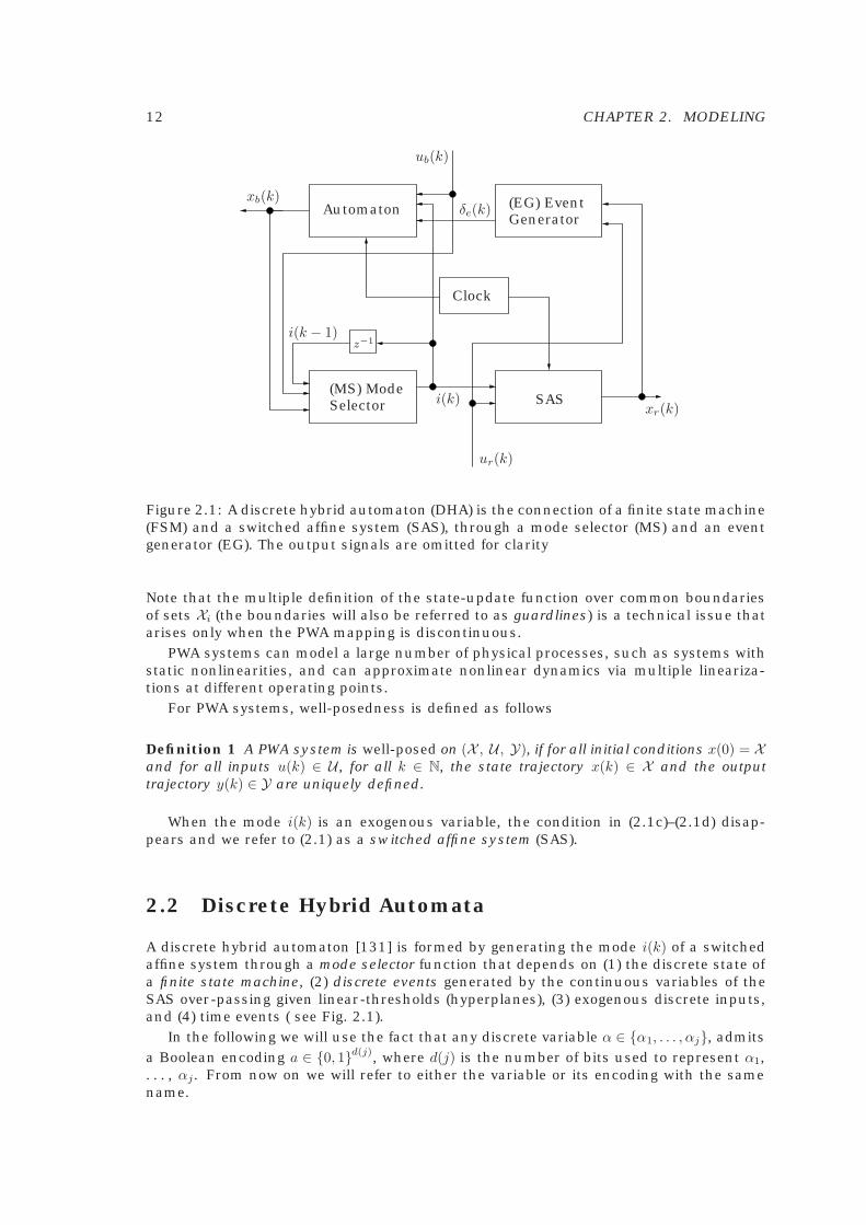
Figure 2.1: A discrete hybrid automaton (DHA) is the connection of a finite state machine(FSM) and a switched affine system (SAS), through a mode selector (MS) and an eventgenerator (EG). The output signals are omitted for clarity
Note that the multiple definition of the state-update function over common boundariesof sets Xi (the boundaries will also be referred to as guardlines) is a technical issue thatarises only when the PWA mapping is discontinuous.
PWA systems can model a large number of physical processes, such as systems withstatic nonlinearities, and can approximate nonlinear dynamics via multiple lineariza-tions at different operating points.
For PWA systems, well-posedness is defined as follows
Definition 1 A PWA system is well-posed on (X , U , Y), if for all initial conditions x(0) = Xand for all inputs u(k) ∈ U , for all k ∈ N, the state trajectory x(k) ∈ X and the outputtrajectory y(k) ∈ Y are uniquely defined.
When the mode i(k) is an exogenous variable, the condition in (2.1c)–(2.1d) disap-pears and we refer to (2.1) as a switched affine system (SAS).
2.2 Discrete Hybrid Automata
A discrete hybrid automaton [131] is formed by generating the mode i(k) of a switchedaffine system through a mode selector function that depends on (1) the discrete state ofa finite state machine, (2) discrete events generated by the continuous variables of theSAS over-passing given linear-thresholds (hyperplanes), (3) exogenous discrete inputs,and (4) time events ( see Fig. 2.1).
In the following we will use the fact that any discrete variable α ∈ {α1, . . . , αj}, admitsa Boolean encoding a ∈ {0, 1}d(j), where d(j) is the number of bits used to represent α1,. . . , αj. From now on we will refer to either the variable or its encoding with the samename.
2.2. DISCRETE HYBRID AUTOMATA 13
2.2.1 Switched Affine System (SAS)
A switched affine system is a collection of linear affine systems:
x′r(k) = Ai(k)xr(k) +Bi(k)ur(k) + fi(k), (2.2a)
yr(k) = Ci(k)xr(k) +Di(k)ur(k) + gi(k), (2.2b)
where k ∈ Z+ is the time indicator, ′ denotes the successor operator (x′r(k) = xr(k + 1)),
xr ∈ Xr ⊆ Rnr is the continuous state vector, ur ∈ Ur ⊆ R
mr is the exogenous continuousinput vector, yr ∈ Yr ⊆ R
pr is the continuous output vector, {Ai, Bi, fi, Ci, Di, gi}i∈I is acollection of matrices of opportune dimensions, and the mode i(k) ∈ I � {1, . . . , s} is aninput signal that chooses the affine state update dynamics. A SAS of the form (2.2) pre-serves the value of the state when a switch occurs, however it is possible to implementreset maps on a SAS, as shown in [131]. A SAS can be rewritten as the combination oflinear terms and if-then-else rules: The state-update equation (2.2a) is equivalent to
z1(k) ={A1xr(k) +B1ur(k) + f1, if (i(k) = 1),0, otherwise, (2.3a)
...
zs(k) ={Asxr(k) +Bsur(k) + fs, if (i(k) = s),0, otherwise, (2.3b)
x′r(k) =s∑
i=1
zi(k), (2.3c)
where zi(k) ∈ Rnr , i = 1, . . . , s, and (2.2b) admits a similar transformation.
2.2.2 Event Generator (EG)
An event generator is a mathematical object that generates a logic signal according tothe satisfaction of a linear (or affine) constraint:
δe(k) = fH(xr(k), ur(k), k), (2.4)
where fH : Xr × Ur × Z≥0 → D ⊆ {0, 1}ne is a vector of descriptive functions of a linearhyperplane, and Z≥0 � {0, 1, . . .} is the set of nonnegative integers. In particular, timeevents are modeled as: [δi
e(k) = 1]↔ [kTs ≥ t0], where Ts is the sampling time and t0 is agiven time, while threshold events are modeled as: [δi
e(k) = 1] ↔ [aTxr(k) + bTur(k) ≤ c],where i denotes the i-th component of a vector.
2.2.3 Finite State Machine (FSM )
A finite state machine1 (or automaton) is a discrete dynamic process that evolves ac-cording to a logic state update function:
x′b(k) = fB(xb(k), ub(k), δe(k)), (2.5a)
where xb ∈ Xb ⊆ {0, 1}nb is the Boolean state, ub ∈ Ub ⊆ {0, 1}mb is the exogenous Booleaninput, δe(k) is the endogenous input coming from the EG, and fB : Xb × Ub ×D → Xb is adeterministic logic function. A FSM can be conveniently represented using an orientedgraph. A FSM may also have an associated Boolean output
yb(k) = gB(xb(k), ub(k), δe(k)), (2.5b)
1In this notes we will only refer to synchronous finite state machines, where the transitions may happenonly at sampling times. The adjective synchronous will be omitted for brevity.
14 CHAPTER 2. MODELING
¬δ3
δ1 ∧ ub2
δ1 ∧ ¬ub2
δ2
δ3 ∧ ub1
¬δ1
¬ub1 ∧ δ3 ¬δ2
Red
Green Blue
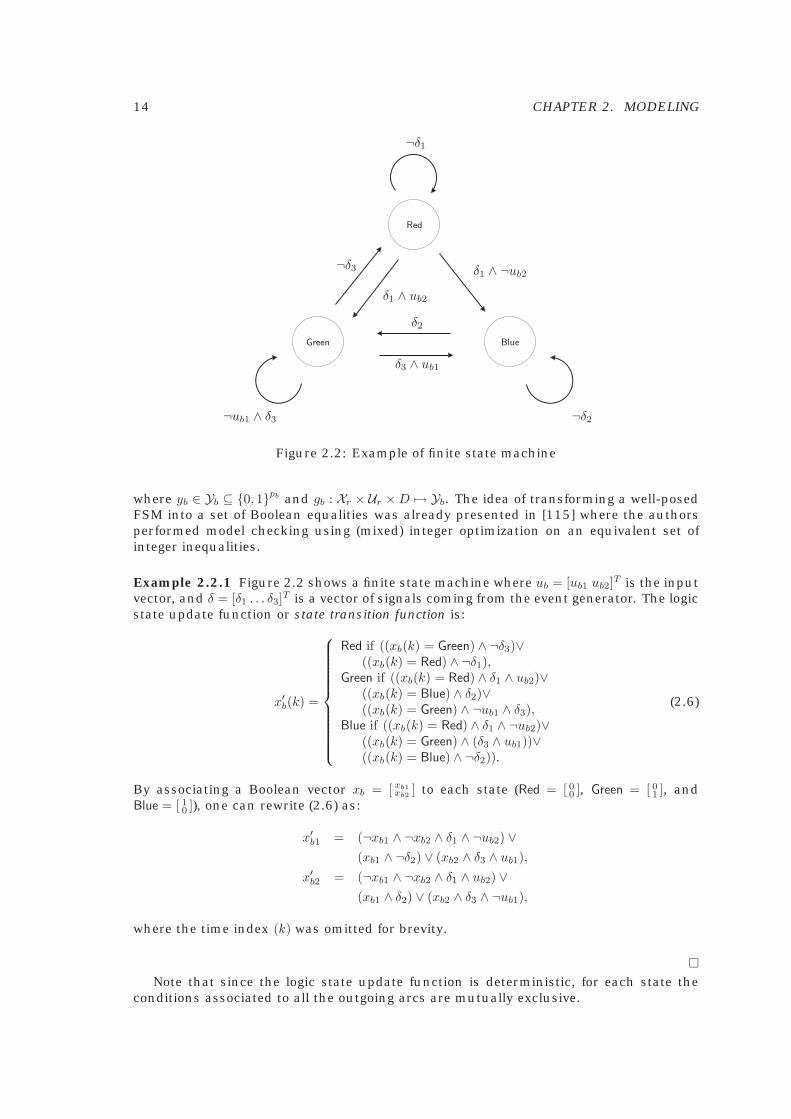
Figure 2.2: Example of finite state machine
where yb ∈ Yb ⊆ {0, 1}pb and gb : Xr × Ur ×D → Yb. The idea of transforming a well-posedFSM into a set of Boolean equalities was already presented in [115] where the authorsperformed model checking using (mixed) integer optimization on an equivalent set ofinteger inequalities.
Example 2.2.1 Figure 2.2 shows a finite state machine where ub = [ub1 ub2]T is the inputvector, and δ = [δ1 . . . δ3]T is a vector of signals coming from the event generator. The logicstate update function or state transition function is:
x′b(k) =
Red if ((xb(k) = Green) ∧ ¬δ3)∨((xb(k) = Red) ∧ ¬δ1),
Green if ((xb(k) = Red) ∧ δ1 ∧ ub2)∨((xb(k) = Blue) ∧ δ2)∨((xb(k) = Green) ∧ ¬ub1 ∧ δ3),
Blue if ((xb(k) = Red) ∧ δ1 ∧ ¬ub2)∨((xb(k) = Green) ∧ (δ3 ∧ ub1))∨((xb(k) = Blue) ∧ ¬δ2)).
(2.6)
By associating a Boolean vector xb = [ xb1xb2 ] to each state (Red = [ 0
0 ], Green = [ 01 ], and
Blue = [ 10 ]), one can rewrite (2.6) as:
x′b1 = (¬xb1 ∧ ¬xb2 ∧ δ1 ∧ ¬ub2) ∨(xb1 ∧ ¬δ2) ∨ (xb2 ∧ δ3 ∧ ub1),
x′b2 = (¬xb1 ∧ ¬xb2 ∧ δ1 ∧ ub2) ∨(xb1 ∧ δ2) ∨ (xb2 ∧ δ3 ∧ ¬ub1),
where the time index (k) was omitted for brevity.
�Note that since the logic state update function is deterministic, for each state the
conditions associated to all the outgoing arcs are mutually exclusive.
2.2. DISCRETE HYBRID AUTOMATA 15
2.2.4 Mode Selector (MS)
The logic state xb(k), the Boolean inputs ub(k), and the events δe(k) select the dynamicmode i(k) of the SAS through a Boolean function fM : Xb×Ub×D → I, which is thereforecalled mode selector. The output of this function
i(k) = fM(xb(k), ub(k), δe(k)) (2.7)
is called active mode. We say that a mode switch occurs at step k if i(k) �= i(k − 1). Notethat, in contrast to continuous-time hybrid models, where switches can occur at anytime, in our discrete-time setting a mode switch can only occur at sampling instants.
2.2.5 DHA Trajectories
For a given initial condition[
xr(0)xb(0)
]∈ Xr × Xb, and input
[ur(k)ub(k)
]∈ Ur × Ub, k ∈ Z≥0, the
state trajectory x(k), k ∈ Z≥0 of the system is recursively computed as follows:
1. Initialization: x(0) =[
xr(0)xb(0)
];
2. Recursion:
(a) δe(k) = fH(xr(k), ur(k), k);
(b) i(k) = fM(xb(k), ub(k), δe(k));
(c) yr(k) = Ci(k)xr(k) +Di(k)ur(k) + gi(k);
(d) yb(k) = gB(xb(k), ub(k), δe(k));
(e) x′r(k) = Ai(k)xr(k) +Bi(k)ur(k) + fi(k);
(f) x′b(k) = fB(xb(k), ub(k), δe(k)).
Definition 2 A DHA is well-posed on Xr × Xb, Ur × Ub, Yr × Yb, if for all initial conditions
x(0) =[
xr(0)xb(0)
]∈ Xr × Xb, and for all inputs u(k) =
[ur(k)ub(k)
]∈ Ur × Ub, for all k ∈ Z≥0, the
state trajectory x(k) ∈ Xr × Xb and output trajectory y(k) =[
yr(k)yb(k)
]∈ Yr × Yb are uniquely
defined.
Definition 2 will be used for other types of hybrid models that we will introduce later.In general a hybrid model may not be well-posed, either because the trajectories stopafter a finite time (for instance, the state vector leaves the set Xr×Xb) or because of non-determinism (the successor x′r(k), x
′b(k) may be multiply defined). Note that trajectories
of DHA are deterministic.DHA modes are a subclass of Hybrid Automata (HA) [3], the main difference is in
the time model, DHA admit time in the natural numbers, while in HA the time is areal number. Moreover DHA models do not allow instantaneous transitions, and aredeterministic, opposed to HA where any enabled transition may occur in zero time.This has two consequences (i) DHA do not admit live-locks (infinite switches in zerotime), (ii) DHA do not admit Zeno behaviors (infinite switches in finite time). Finallyin DHA models, guards, reset maps and continuous dynamics are limited to linear (oraffine) functions. However, working with discrete-time models allows the developmentof several analysis and synthesis tools, as later reported in Chapters 3 and 4.
16 CHAPTER 2. MODELING
2.3 Discrete Hybrid Automata and Piecewise Affine Sys-tems
This section highlights the relationships between the classes of DHA and PWA systemsintroduced in the previous sections.
Definition 3 Let Σ1, Σ2 be hybrid models, whose inputs are u1(k) ∈ U1 ⊆ U , u2(k) ∈ U2 ⊆ Uand outputs y1(k) ∈ Y1 ⊆ Y, y2(k) ∈ Y2 ⊆ Y, k ∈ Z≥0. Let x1(k) ∈ X1 ⊆ X be the state of Σ1
and x2(k) ∈ X2 ⊆ X the state of Σ2, k ∈ Z≥0. The hybrid models Σ1 and Σ2 are equivalenton X , U , Y, X ⊆ X1∩X2, U ⊆ U1∩U2, Y ⊆ Y1∩Y2 if for all initial conditions x1(0) = x2(0) ∈ X ,and for all u1(k) = u2(k) ∈ U , the output trajectories coincides, i.e. y1(k) = y2(k) andx2(k) = x1(k) at all steps k ∈ Z≥0.
Lemma 1 Let ΣPWA be a well-posed PWA model defined on a set of states X ⊆ Rn, a set
of inputs U ⊆ Rm, and a set of outputs Y ⊆ R
p. Then it can be rewritten as an equivalentwell-posed DHA model ΣDHA on U ,X ,Y.
Proof. Equations (2.1a)–(2.1b) are the modes of the SAS, the constraints Hix + Jiu ≤ Ki,i = 1, . . . , s are the defining hyperplanes fH(·) of the EG, and the MS is defined by (2.1c),namely if all the events associated to the hyperplanes of Hjx + Jju ≤ Kj are satisfiedthen i(k) = j. �
2.4 Logic and Mixed-Integer Inequalities
Despite the fact that DHA are rich of expressiveness and are therefore quite suitablefor modeling and simulating hybrid dynamical systems, they are not directly suitablefor solving synthesis and analysis problems, due to their heterogeneous discrete andcontinuous nature. In this section we want to describe how DHA can be translated intodifferent hybrid models that are more suitable for computations. We highlight the maintechniques of the translation process, by generalizing several results appeared in theliterature [31,52,54,81,91,109,112,119,133,135,136].
2.4.1 Logical Functions
Boolean functions can be equivalently expressed by inequalities [54].In order to introduce our notation, we recall here some basic definitions of Boolean
algebra. A variable X is a Boolean variable if X ∈ {0, 1}. A Boolean expression is induc-tively defined2 by the grammar
φ ::= X |¬φ1|φ1 ∨ φ2|φ1 ⊕ φ2|φ1 ∧ φ2|φ1 ← φ2|φ1 → φ2|φ1 ↔ φ2|(φ1),
(2.8)
where X is a Boolean variable, and the logic operators ¬ (not), ∨ (or), ∧ (and), ← (impliedby),→ (implies),↔ (iff) have the usual semantics. A Boolean expression is in conjunctivenormal form (CNF) or product of sums if it can be written according to the followinggrammar:
φ ::= ψ|φ ∧ ψ, (2.9)
ψ ::= ψ1 ∨ ψ2|¬X |X, (2.10)
where ψ are called terms of the product, and X are the terms of the sum ψ. A CNFis minimal if it has the minimum number of terms of product and each term has the
2For the sake of simplicity, we are neglecting precedence.
2.4. LOGIC AND MIXED-INTEGER INEQUALITIES 17
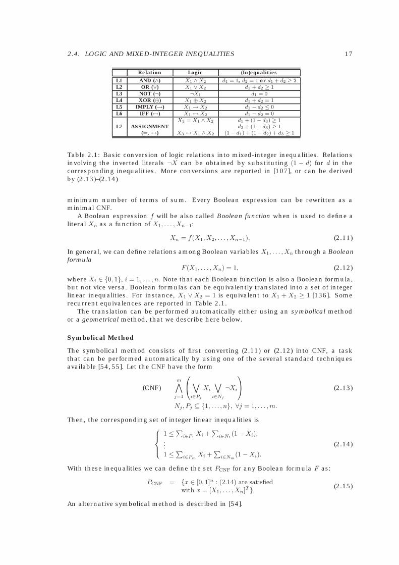
Relation Logic (In)equalities
L1 AND (∧) X1 ∧X2 d1 = 1, d2 = 1 or d1 + d2 ≥ 2L2 OR (∨) X1 ∨X2 d1 + d2 ≥ 1L3 NOT (¬) ¬X1 d1 = 0L4 XOR (⊕) X1 ⊕X2 d1 + d2 = 1L5 IMPLY (→) X1 → X2 d1 − d2 ≤ 0L6 IFF (↔) X1 ↔ X2 d1 − d2 = 0
X3 = X1 ∧X2 d1 + (1 − d3) ≥ 1L7 ASSIGNMENT d2 + (1 − d3) ≥ 1
(=, ↔) X3 ↔ X1 ∧X2 (1 − d1) + (1− d2) + d3 ≥ 1
Table 2.1: Basic conversion of logic relations into mixed-integer inequalities. Relationsinvolving the inverted literals ¬X can be obtained by substituting (1 − d) for d in thecorresponding inequalities. More conversions are reported in [107], or can be derivedby (2.13)–(2.14)
minimum number of terms of sum. Every Boolean expression can be rewritten as aminimal CNF.
A Boolean expression f will be also called Boolean function when is used to define aliteral Xn as a function of X1, . . . , Xn−1:
Xn = f(X1, X2, . . . , Xn−1). (2.11)
In general, we can define relations among Boolean variables X1, . . . , Xn through a Booleanformula
F (X1, . . . , Xn) = 1, (2.12)
where Xi ∈ {0, 1}, i = 1, . . . , n. Note that each Boolean function is also a Boolean formula,but not vice versa. Boolean formulas can be equivalently translated into a set of integerlinear inequalities. For instance, X1 ∨X2 = 1 is equivalent to X1 + X2 ≥ 1 [136]. Somerecurrent equivalences are reported in Table 2.1.
The translation can be performed automatically either using an symbolical methodor a geometrical method, that we describe here below.
Symbolical Method
The symbolical method consists of first converting (2.11) or (2.12) into CNF, a taskthat can be performed automatically by using one of the several standard techniquesavailable [54,55]. Let the CNF have the form
(CNF)m∧
j=1
∨
i∈Pj
Xi
∨i∈Nj
¬Xi
(2.13)
Nj , Pj ⊆ {1, . . . , n}, ∀j = 1, . . . ,m.
Then, the corresponding set of integer linear inequalities is
1 ≤∑
i∈P1Xi +
∑i∈N1
(1 −Xi),...1 ≤
∑i∈Pm
Xi +∑
i∈Nm(1−Xi).
(2.14)
With these inequalities we can define the set PCNF for any Boolean formula F as:
PCNF = {x ∈ [0, 1]n : (2.14) are satisfiedwith x = [X1, . . . , Xn]T }. (2.15)
An alternative symbolical method is described in [54].
18 CHAPTER 2. MODELING
Geometrical Method
The geometrical method consists of two steps (see e.g. [111]). First, the set of points in[0, 1]n satisfying (2.11) or (2.12) is computed (for this reason, the method was also calledtruth table method in [111]). Each row of the truth table is associated with a vertex ofthe hypercube {0, 1}n. The vertices are collected in a set V of valid points, all the otherpoints {0, 1}n \ V are called invalid. The inequalities representing the Boolean formulaare obtained by computing the convex hull of V , for which several tools are available(see e.g. [77]). We therefore define
PCH = {x ∈ [0, 1]n : x ∈ conv(V )}. (2.16)
Although PCH and PCNF contain the same integer points, i.e. (PCH ∩ {0, 1}n) = (PCNF ∩{0, 1}n), in general the set PCH ⊆ PCNF, since conv(V ) is the smallest set containing allinteger feasible points. However, there exist Boolean formulas, for which PCH �= PCNF
3.Conditions for which PCH = PCNF are currently a topic of research.
2.4.2 Continuous-Logic Interfaces
Events of the form (2.4) can be equivalently expressed as
f iH(xr(k), ur(k), k) ≤M i(1− δi
e), (2.17a)
f iH(xr(k), ur(k), k) > miδi
e, i = 1, . . . , ne, (2.17b)
where M i, mi are upper and lower bounds, respectively, on fiH(xr(k), ur(k), k). As we
will point out in Section 2.5, sometimes from a computational point of view, it may beconvenient to have a system of inequalities without strict inequalities. In this case wewill follow the common practice [136] to replace the strict inequality (2.17b) as
f iH(xr(k), ur(k), k) ≥ ε+ (mi − ε)δi
e, (2.17c)
where ε is a small positive scalar, e.g., the machine precision, although the equivalencedoes not hold for 0 < f i
H(xr(k), ur(k), k) < ε, i.e., for the numbers in the interval (0, ε) thatcannot be represented in a computer.
The most common logic to continuous interface is the if-then-else construct
IF δ THEN z = a′1x+ b′1u+ f1 ELSE z = a′2x+ b′2u+ f2, (2.18)
where δ ∈ {0, 1}, z ∈ R, x ∈ Rn, u ∈ R
m, and a1, b1, f1, a2, b2, f2 are constants of suitabledimensions. The if-then-else construct (2.18) can be translated into [37]
(m2 −M1)δ + z ≤ a′2x+ b′2u+ f2, (2.19a)
(m1 −M2)δ − z ≤ −a′2x− b′2u− f2, (2.19b)
(m1 −M2)(1− δ) + z ≤ a′1x+ b′1u+ f1, (2.19c)
(m2 −M1)(1− δ)− z ≤ −a′1x− b′1u− f1, (2.19d)
where Mi, mi are upper and lower bounds on aix + biu + fi, i = 1, 2. Note that whena2 = 0, b2 = 0, f2 = 0, relations (2.18)–(2.19) model the real product z = δ · (a′1x + b′1u+ f)described in [136].
2.5 Mixed Logical Dynamical Systems
Mixed logical dynamical (MLD) systems are computationally oriented representationsof hybrid systems that consist of a collection of linear difference equations involving
3For example (X1 ∨X2) ∧ (X1 ∨X3) ∧ (X2 ∨X3).
2.5. MIXED LOGICAL DYNAMICAL SYSTEMS 19
both real and (0-1) variables, subject to a set of linear inequalities [31]. Typically, MLDmodels are obtained by starting with a DHA representation of a given hybrid process,according to the techniques described in the previous section.
An MLD system is described by the following relations:
x′(k) = Ax(k) +B1u(k) +B2δ(k) +B3z(k) +B5, (2.20a)
y(k) = Cx(k) +D1u(k) +D2δ(k) +D3z(k) +D5, (2.20b)
E2δ(k) + E3z(k) ≤ E1u(k) + E4x(k) + E5, (2.20c)
E2δ(k) + E3z(k) = E1u(k) + E4x(k) + E5. (2.20d)
where x ∈ Rnr×{0, 1}nb is a vector of continuous and binary states, u ∈ R
mr×{0, 1}mb arethe inputs, y ∈ R
pr × {0, 1}pb the outputs, δ ∈ {0, 1}rb, z ∈ Rrr represent auxiliary binary
and continuous variables, respectively, and A, B1, B2, B3, C, D1, D2, D3, E1,. . . ,E5 andE1,. . . ,E5 are matrices of suitable dimensions. Given the current state x(k) and inputu(k), the time-evolution of (2.20) is determined by solving δ(k) and z(k) from (2.20c)–(2.20d), and then updating x′(k) and y(k) from (2.20a)–(2.20b).
We assume that system (2.20) is completely well-posed [31], which means that forall x(k), u(k) within a given bounded set the variables δ(k), z(k) are defined by (2.20c)–(2.20d) in a unique way4. This allows assuming that x(k + 1) and y(k) are uniquelydefined once x(k), u(k) are given, and therefore that x- and y-trajectories exist and areuniquely determined by the initial state x(0) and input signal u(0), u(1), . . .. It is clearthat the well-posedness assumption stated above is usually guaranteed by the proce-dure used to generate the linear inequalities (2.20c), and therefore this hypothesis istypically fulfilled by MLD relations derived from modeling real-world plants. Neverthe-less, a numerical test for well-posedness is reported in [31, Appendix 1].
The equations and inequalities obtained with the methods presented in Sections 2.4.1and 2.4.2 typically contribute to defining the MLD model (2.20). Since the problems ofsynthesis and analysis of MLD models are tackled by optimization techniques, we havereplaced strict inequalities as in (2.17b) by non-strict inequalities as in (2.17c)5. Asobserved before, indeed strict inequalities of the form a′x > b can be approximated bya′x ≥ b+ ε where ε is a small positive scalar, e.g., the machine precision (which dependson the number of bits used for representing real numbers), although the equivalencedoes not hold for 0 < a′x− b < ε, that is for the numbers in the interval (0, ε) that cannotbe represented in the machine).
Note that the constraints (2.20c) allow one to specify additional linear constraints oncontinuous variables (e.g., constraints over physical variables of the system), and logicconstraints over Boolean variables. The ability to include constraints, constraint priori-tization, and heuristics adds to the expressiveness and generality of the MLD framework.Note also that despite the fact that the description (2.20) seems to be linear, clearly thenonlinearity is concentrated in the integrality constraints over binary variables. Thefollowing simple example illustrates the technique.
Example 2.5.1 Consider the following simple switched scalar system [31]
x(k + 1) ={
0.8x(k) + u(k) if x(k) ≥ 0−0.8x(k) + u(k) if x(k) < 0 (2.21)
where x(k) ∈ [−10, 10], and u(k) ∈ [−1, 1]. The condition x(k) ≥ 0 can be associated to abinary variable δ(k) such that
[δ(k) = 1] ↔ [x(k) ≥ 0] . (2.22)
4For a more general definition of well-posedness, see [31].5One may also explicitly include in (2.20) strict inequality constraints E2δ(k) + E3z(k) < E1u(k) + E4x(k) +
E5.
20 CHAPTER 2. MODELING
By using the transformations (2.17a)–(2.17c), equation (2.22) can be expressed by theinequalities
−mδ(k) ≤ x(k)−m (2.23a)
−(M + ε)δ(k) ≤ −x(k)− ε (2.23b)
where M = −m = 10, and ε is a small positive scalar. Then (2.21) can be rewritten as
x(t+ 1) = 1.6δ(k)x(k)− 0.8x(k) + u(k). (2.24)
By defining a new variable z(k) = δ(k)x(k) which, by (2.18)–(2.19) can be expressed as
z(k) ≤ Mδ(k) (2.25a)
z(k) ≥ mδ(k) (2.25b)
z(k) ≤ x(k)−m(1− δ(k)) (2.25c)
z(k) ≥ x(k)−M(1− δ(k)), (2.25d)
the evolution of system (2.21) is ruled by the linear equation
x(t+ 1) = 1.6z(k)− 0.8x(k) + u(k)
subject to the linear constraints (2.23) and (2.25).
Lemma 2 Let ΣDHA be a well-posed DHA model defined on a set of states X ⊆ Rn, a set
of inputs U ⊆ Rm, and a set of outputs Y ⊆ R
p. Then for any bounded X , U , there exists awell posed MLD model ΣMLD equivalent to ΣDHA on X , U , Y.
Proof. Directly follows from Sections 2.4.1, 2.4.2, (2.3). �Finally we recall that the MLD model is similar to the model presented in [67] for
verification of safety properties as they both aim at translating a hybrid system in a setof mixed integer linear equalities and inequalities using similar techniques.
2.6 Other Computational Models and Further Equiva-lences
In the previous section we showed the equivalence relations between DHA, PWA andMLD systems. In this section, we review other existing models of linear hybrid systemsand show further relationships with DHA.
2.6.1 Linear Complementarity Systems
Linear complementarity (LC) systems are given in discrete-time by the equations
x′(k) = Ax(k) +B1u(k) +B2w(k), (2.26a)
y(k) = Cx(k) +D1u(k) +D2w(k), (2.26b)
v(k) = E1x(k) + E2u(k) + E3w(k) + E4, (2.26c)
0 ≤ v(k) ⊥ w(k) ≥ 0, (2.26d)
with v(k), w(k) ∈ Rq and where ⊥ denotes the orthogonality of vectors (i.e. v(k)⊥w(k)
means that vT (k)w(k) = 0). We call v(k) and w(k) the complementarity variables. A, Bi,C, Di and Ei are real matrices [53,87,88,126,134].
2.6. OTHER COMPUTATIONAL MODELS AND FURTHER EQUIVALENCES 21
2.6.2 Extended Linear Complementarity (ELC) Systems
In [62,63,65] it has been shown that several types of hybrid systems can be modeled asextended linear complementarity (ELC) systems:
x(k + 1) = Ax(k) +B1u(k) +B2w(k) (2.27a)
y(k) = Cx(k) +D1u(k) +D2w(k) (2.27b)
E1x(k) + E2u(k) + E3w(k) � g4 (2.27c)p∑
i=1
∏j∈φi
(g4 − E1x(k)− E2u(k)− E3w(k)
)j
= 0, (2.27d)
where w(k) ∈ Rr is a vector of auxiliary variables. Condition (2.27d) is equivalent to
∏j∈φi
(g4 − E1x(k)− E2u(k)− E3w(k)
)j
= 0∀i ∈ {1, 2, . . . , p} (2.28)
due to the inequality conditions (2.27c). This implies that (2.27c)–(2.27d) can be con-sidered as a system of linear inequalities (i.e. (2.27c)), where there are p groups of linearinequalities (one group for each index set φi) such that in each group at least one in-equality should hold with equality. Note that LC systems are a particular case of ELCsystems.
2.6.3 Max-Min-Plus-Scaling (MMPS) Systems
In [65] a class of discrete event systems has been introduced that can be modelled usingthe operations maximization, minimization, addition and scalar multiplication. Expres-sions that are built using these operations are called max-min-plus-scaling (MMPS)expressions.
Definition 4 (Max-min-plus-scaling expression) A max-min-plus-scaling expression fof the variables x1, . . . , xn is defined by the grammar6
f := xi|α|max(fk, fl)|min(fk, fl)|fk + fl|βfk (2.29)
with i ∈ {1, 2, . . . , n}, α, β ∈ R, and where fk, fl are again MMPS expressions.
A MMPS expression is e.g. 2x1 +4x2−3, min(max(−x1, 2x2), 3x2 +x3). Note that the min op-eration is in fact not explicitly needed in (2.29) since we have min(fk, fl) = −max(−fk,−fl).
MMPS systems are defined by the relations
x(k + 1) =Mx(x(k), u(k), w(k)) (2.30a)
y(k) =My(x(k), u(k), w(k)) (2.30b)
Mc(x(k), u(k), w(k)) � c, (2.30c)
where Mx, My and Mc are MMPS expressions in terms of the components of x(k), theinput u(k) and the auxiliary variables w(k), which are all real-valued.
Despite the fact that MMPS functions are continuous, discontinuous functions canbe modeled through MMPS inequalities. For instance, wi(k) ∈ {0, 1} can be representedby the two inequalities max(wi(k)− 1,−wi(k)) ≥ 0, −max(wi(k)− 1,−wi(k)) ≥ 0. Similarly,in LC models it can be represented by wi(k)(1 − wi(k)) ≤ 0, wi(k) ≥ 0, 1− wi(k) ≥ 0.
6The symbol | stands for OR and the definition is recursive.
22 CHAPTER 2. MODELING
MLD
PWA
?
?
?
?
?
? ?
?
?
LC
ELC
MMPS
DHA
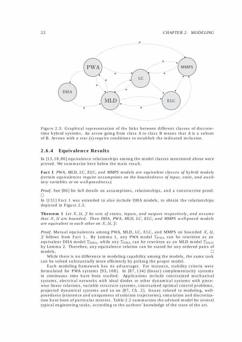
Figure 2.3: Graphical representation of the links between different classes of discrete-time hybrid systems. An arrow going from class A to class B means that A is a subsetof B. Arrows with a star (�) require conditions to establish the indicated inclusion.
2.6.4 Equivalence Results
In [13,18,86] equivalence relationships among the model classes mentioned above wereproved. We summarize here below the main result.
Fact 1 PWA, MLD, LC, ELC, and MMPS models are equivalent classes of hybrid models(certain equivalences require assumptions on the boundedness of input, state, and auxil-iary variables or on well-posedness).
Proof. See [86] for full details on assumptions, relationships, and a constructive proof.�In [131] Fact 1 was extended to also include DHA models, to obtain the relationshipsdepicted in Figure 2.3.
Theorem 1 Let X , U , Y be sets of states, inputs, and outputs respectively, and assumethat X , U are bounded. Then DHA, PWA, MLD, LC, ELC, and MMPS well-posed modelsare equivalent to each other on X , U , Y.
Proof. Mutual equivalences among PWA, MLD, LC, ELC, and MMPS on bounded X , U ,Y follows from Fact 1. By Lemma 1, any PWA model ΣPWA can be rewritten as anequivalent DHA model ΣDHA, while any ΣDHA can be rewritten as an MLD model ΣMLD
by Lemma 2. Therefore, any equivalence relation can be stated for any ordered pairs ofmodels. �
While there is no difference in modeling capability among the models, the same taskcan be solved substantially more efficiently by picking the proper model.
Each modeling framework has its advantages. For instance, stability criteria wereformulated for PWA systems [93, 108]. In [87, 134] (linear) complementarity systemsin continuous time have been studied. Applications include constrained mechanicalsystems, electrical networks with ideal diodes or other dynamical systems with piece-wise linear relations, variable structure systems, constrained optimal control problems,projected dynamical systems and so on [87, Ch. 2]. Issues related to modeling, well-posedness (existence and uniqueness of solution trajectories), simulation and discretiza-tion have been of particular interest. Table 2.2 summarizes the advised model for severaltypical engineering tasks, according to the authors’ knowledge of the state of the art.
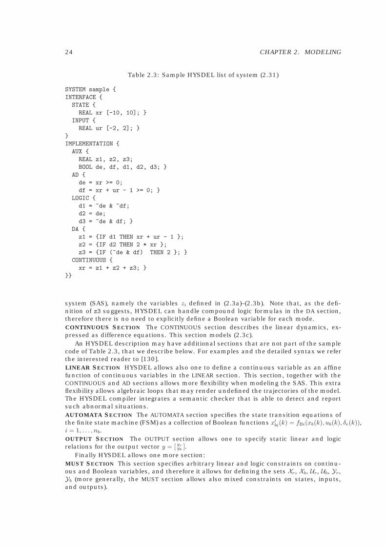
2.7. HYSDEL MODELS 23
Table 2.2: Advised model for each taskTask ModelModeling DHASimulation DHAControl MLD,PWA,MMPSStability PWAVerification PWAIdentification PWAFault Detection MLDEstimation MLD
2.7 HYSDEL Models
A modeling language was proposed in [131] to describe DHA models, called HYbrid Sys-tem DEscription Language (HYSDEL). The HYSDEL description of a DHA is an abstractmodeling step. The associated HYSDEL compiler then translates the description intoseveral computational models, in particular into a MLD using the technique presentedin Section 2.4, and PWA form using either the direct approach of [79] or the indirectapproach that translates the MLD into a PWA of [13]. HYSDEL can generate also asimulator that runs as a function in Matlab.
In this section we show how a DHA system can be modeled in HYSDEL by illustratingthe HYSDEL description of the following DHA system:
SAS: x′r(k) =
xr(k) + ur(k)− 1, if i(k) = 1,2xr(k), if i(k) = 2,2, if i(k) = 3,
(2.31a)
EG:{δe(k) = [xr(k) ≥ 0],δf (k) = [xr(k) + ur(k)− 1 ≥ 0], (2.31b)
MS: i(k) =
1, if[
δe(k)δf (k)
]= [ 0
0 ] ,2, if δe(k) = 1,3, if
[δe(k)δf (k)
]= [ 0
1 ] .(2.31c)
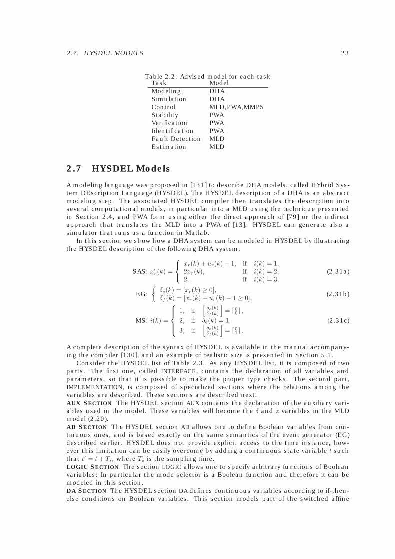
A complete description of the syntax of HYSDEL is available in the manual accompany-ing the compiler [130], and an example of realistic size is presented in Section 5.1.
Consider the HYSDEL list of Table 2.3. As any HYSDEL list, it is composed of twoparts. The first one, called INTERFACE, contains the declaration of all variables andparameters, so that it is possible to make the proper type checks. The second part,IMPLEMENTATION, is composed of specialized sections where the relations among thevariables are described. These sections are described next.AUX SECTION The HYSDEL section AUX contains the declaration of the auxiliary vari-ables used in the model. These variables will become the δ and z variables in the MLDmodel (2.20).AD SECTION The HYSDEL section AD allows one to define Boolean variables from con-tinuous ones, and is based exactly on the same semantics of the event generator (EG)described earlier. HYSDEL does not provide explicit access to the time instance, how-ever this limitation can be easily overcome by adding a continuous state variable t suchthat t′ = t+ Ts, where Ts is the sampling time.LOGIC SECTION The section LOGIC allows one to specify arbitrary functions of Booleanvariables: In particular the mode selector is a Boolean function and therefore it can bemodeled in this section.DA SECTION The HYSDEL section DA defines continuous variables according to if-then-else conditions on Boolean variables. This section models part of the switched affine
24 CHAPTER 2. MODELING
Table 2.3: Sample HYSDEL list of system (2.31)
SYSTEM sample {INTERFACE {STATE {
REAL xr [-10, 10]; }INPUT {
REAL ur [-2, 2]; }}IMPLEMENTATION {AUX {
REAL z1, z2, z3;BOOL de, df, d1, d2, d3; }
AD {de = xr >= 0;df = xr + ur - 1 >= 0; }
LOGIC {d1 = ~de & ~df;d2 = de;d3 = ~de & df; }
DA {z1 = {IF d1 THEN xr + ur - 1 };z2 = {IF d2 THEN 2 * xr };z3 = {IF (~de & df) THEN 2 }; }
CONTINUOUS {xr = z1 + z2 + z3; }
}}
system (SAS), namely the variables zi defined in (2.3a)–(2.3b). Note that, as the defi-nition of z3 suggests, HYSDEL can handle compound logic formulas in the DA section,therefore there is no need to explicitly define a Boolean variable for each mode.CONTINUOUS SECTION The CONTINUOUS section describes the linear dynamics, ex-pressed as difference equations. This section models (2.3c).
An HYSDEL description may have additional sections that are not part of the samplecode of Table 2.3, that we describe below. For examples and the detailed syntax we referthe interested reader to [130].LINEAR SECTION HYSDEL allows also one to define a continuous variable as an affinefunction of continuous variables in the LINEAR section. This section, together with theCONTINUOUS and AD sections allows more flexibility when modeling the SAS. This extraflexibility allows algebraic loops that may render undefined the trajectories of the model.The HYSDEL compiler integrates a semantic checker that is able to detect and reportsuch abnormal situations.AUTOMATA SECTION The AUTOMATA section specifies the state transition equations ofthe finite state machine (FSM) as a collection of Boolean functions x′bi(k) = fBi(xb(k), ub(k), δe(k)),i = 1, . . . , nb.OUTPUT SECTION The OUTPUT section allows one to specify static linear and logicrelations for the output vector y = [ yr
yb ].Finally HYSDEL allows one more section:
MUST SECTION This section specifies arbitrary linear and logic constraints on continu-ous and Boolean variables, and therefore it allows for defining the sets Xr, Xb, Ur, Ub, Yr,Yb (more generally, the MUST section allows also mixed constraints on states, inputs,and outputs).
2.8. A SIMPLE EXAMPLE 25
Thanks to the equivalences mentioned in the previous section, it is clear that HYS-DEL is a tool that allows generating several different hybrid models of a given hybridsystem. In particular, HYSDEL generates MLD models, which can be immediately (andefficiently) translated into PWA systems [13, 79], or LC/ELC/MMPS systems using theconstructive methods reported in [86].
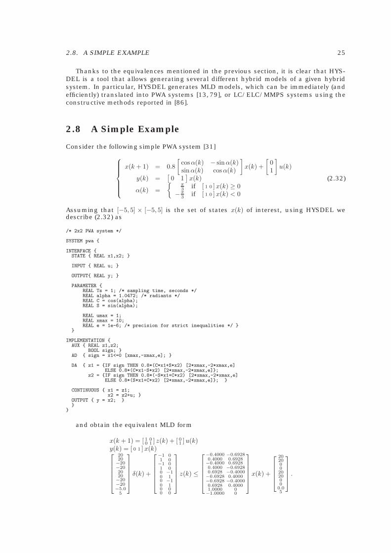
2.8 A Simple Example
Consider the following simple PWA system [31]
x(k + 1) = 0.8[
cosα(k) − sinα(k)sinα(k) cosα(k)
]x(k) +
[01
]u(k)
y(k) =[0 1
]x(k)
α(k) ={
π3 if [ 1 0 ]x(k) ≥ 0−π
3 if [ 1 0 ]x(k) < 0
(2.32)
Assuming that [−5, 5] × [−5, 5] is the set of states x(k) of interest, using HYSDEL wedescribe (2.32) as
/* 2x2 PWA system */
SYSTEM pwa {
INTERFACE {STATE { REAL x1,x2; }
INPUT { REAL u; }
OUTPUT{ REAL y; }
PARAMETER {REAL Ts = 1; /* sampling time, seconds */REAL alpha = 1.0472; /* radiants */REAL C = cos(alpha);REAL S = sin(alpha);
REAL umax = 1;REAL xmax = 10;REAL e = 1e-6; /* precision for strict inequalities */ }
}
IMPLEMENTATION {AUX { REAL z1,z2;
BOOL sign; }AD { sign = x1<=0 [xmax,-xmax,e]; }
DA { z1 = {IF sign THEN 0.8*(C*x1+S*x2) [2*xmax,-2*xmax,e]ELSE 0.8*(C*x1-S*x2) [2*xmax,-2*xmax,e]};
z2 = {IF sign THEN 0.8*(-S*x1+C*x2) [2*xmax,-2*xmax,e]ELSE 0.8*(S*x1+C*x2) [2*xmax,-2*xmax,e]}; }
CONTINUOUS { x1 = z1;x2 = z2+u; }
OUTPUT { y = x2; }}
}
and obtain the equivalent MLD form
x(k + 1) = [ 1 00 1 ] z(k) + [ 0
1 ]u(k)y(k) = [ 0 1 ]x(k)
2020−20−202020−20−20−5.0
5
δ(k) +
−1 01 0−1 01 00 −10 10 −10 10 00 0
z(k) ≤
−0.4000 −0.69280.4000 0.6928−0.4000 0.69280.4000 −0.69280.6928 −0.4000−0.6928 0.4000−0.6928 −0.40000.6928 0.40001.0000 0−1.0000 0
x(k) +
202000202000
0.05
.

26 CHAPTER 2. MODELING
2.9 Identification of Hybrid Systems
Finally, we mention that identification techniques for obtaining piecewise affine models(or parts of models) from input/output data were recently developed in [12,21,73,123].
Chapter 3
Controller Synthesis
3.1 Introduction
Controlling a system means to choose the command input signals so that the outputsignals tracks some desired reference trajectories. The control problem can be tackledin several ways, according to the model type and control objective.
The problem of determining optimal control laws for hybrid systems has been widelyinvestigated in recent years and many results can be found in the control and computerscience literature. For continuous-time hybrid systems, most of the literature is focusedon the study of necessary conditions for a trajectory to be optimal [116,129], and on thecomputation of optimal/suboptimal solutions by means of dynamic programming or themaximum principle [46,47,82,85,100,121,122,138]. For determining the optimal feed-back control law some of these techniques require the discretization of the state spacein order to solve the corresponding Hamilton-Jacobi-Bellman equations. In [82] theauthors use a hierarchical decomposition approach to break down the overall probleminto smaller ones. In so doing, discretization is not involved and the main computationalcomplexity arises from a higher-level nonlinear programming problem.
Optimal quadratic control of piecewise linear and hybrid systems is addressed in[85, 120], where the authors derive bounds on the solution to the associated Hamilton-Jacobi-Bellman inequalities, which are computable by solving convex optimization prob-lems (linear matrix inequalities [120] or finite-dimensional linear programming [85]). Inthe case of switched linear systems composed by stable autonomous dynamics, in [27]the authors proved that the control law is a state-feedback and there exists a numericalprocedure to compute the regions of the state space where the i-th switch should occur.
The hybrid optimal control problem becomes less complex when the dynamics isexpressed in discrete-time or as discrete-events [49]. In the area of intelligent manu-facturing and queuing systems, for example, one frequently faces scheduling problems.The goal of scheduling is to accomplish a given set of tasks (also identified as jobs) soas to optimize a meaningful performance criterion. Since the jobs to be scheduled usu-ally involve some dynamics, the problem is hybrid. The dynamics taken into account inscheduling problems are generally very simple (often just of integral type, correspondingto timed events [50, 105]). Optimization of hybrid processes through dynamic simula-tion is also proposed in [114]. Here, the authors use mixed-integer linear programming(MILP) to obtain a candidate switching sequence. A standard scheduling problem isthen solved for the fixed sequence.
For discrete-time linear hybrid systems, in [31] the authors showed how mixed-integer quadratic programming (MIQP) can be efficiently used to determine optimal con-trol sequences. It was also shown that when optimal control is implemented in a reced-ing horizon fashion by repeatedly solving MIQPs on-line, this leads to an asymptoticallystabilizing control law. For those cases where on-line optimization is not viable, [16,17]
27
28 CHAPTER 3. CONTROLLER SYNTHESIS
proposed multiparametric programming as an effective means for synthesizing piece-wise affine optimal controllers, that solve in state-feedback form the finite-time hybridoptimal control problem with criteria based on linear (1-norm, ∞-norm) and quadratic(squared Euclidean norm) performance objectives. Such a control design flow for hybridsystems was applied to several industrial case studies, in particular to automotive prob-lems where the simplicity of the control law is essential for its applicability [14,24,110].
In the discrete-time case, the main source of complexity is the combinatorial num-ber of possible switching sequences. By combining reachability analysis and quadraticoptimization, in Chapter 4 we describe a technique that rules out switching sequencesthat are either not optimal or simply not compatible with the evolution of the dynamicalsystem. An algorithm to optimize switching sequences that has an arbitrary degree ofsuboptimality was presented in [100].
Other approaches for synthesizing controllers for piecewise affine systems using LMIrelaxations was presented in [59], and for min-max-plus-scaling systems in [64].
3.2 Model Predictive Control for Hybrid Systems
For complex constrained multivariable control problems, model predictive control (MPC)has become the accepted standard in the process industries [106, 118]. Here at eachsampling time, starting at the current state, an open-loop optimal control problem issolved over a finite horizon. The optimal command signal is applied to the process onlyduring the following sampling interval. At the next time step a new optimal controlproblem based on new measurements of the state is solved over a shifted horizon. Theoptimal solution relies on a dynamic model of the process, respects all input and out-put constraints, and minimizes a performance figure. This is usually expressed as aquadratic or a linear criterion, so that, for linear prediction models, the resulting op-timization problem can be cast as a quadratic program (QP) or linear program (LP),respectively, for which a rich variety of efficient active-set and interior-point solvers areavailable.
MPC ideas can be applied to control hybrid models. Assume we want the output y(t)to track a reference signal ye, and let xe, ue, δe, ze be a corresponding equilibrium pairfor state, input, and auxiliary variables. Let t be the current time, and x(t) the currentstate. Consider the following optimal control problem
min{v,δ,z}T−1
0
J({v, δ, z}T−10 , x(t)) �
T−1∑k=0
‖Q1(v(k) − ue)‖p+
‖Q2(δ(k|t)− δe)‖p + ‖Q3(z(k|t)− ze)‖p+‖Q4(x(k|t) − xe)‖p + ‖Q5(y(k|t)− ye)‖p (3.1a)
s.t.
x(t|t) = x(t)x(k + 1|t) = Ax(k|t) +B1v(k) +B2δ(k|t) +B3z(k|t) +B5
y(k|t) = Cx(k|t) +D1v(k) +D2δ(k|t) +D3z(k|t) +D5
E2δ(k|t) + E3z(k|t) ≤ E1v(k) + E4x(k|t) + E5
E2δ(k|t) + E3z(k|t) = E1v(k) + E4x(k|t) + E5
umin ≤ v(t+ k) ≤ umax, k = 0, 1, . . . , T − 1xmin ≤ x(t+ k|t) ≤ xmax, k = 1, . . . , T − 1x(T |t) = xe
(3.1b)
where T is the prediction, x(k|t) is the state predicted at time t + k resulting from theinput u(t + k) = v(k) to (2.20) starting from x(0|t) = x(t), umin, umax and xmin, xmax arehard bounds on the inputs and on the states, respectively. In (3.1a), ‖Qx‖p = x′Qx forp = 2 and ‖Qx‖p = ‖Qx‖∞ for p =∞, where
Q1,4 = Q′1,4 � 0, Q2,3,5 = Q′
2,3,5 � 0 (p = 2)Q1−5 nonsingular (p =∞). (3.2)
3.2. MODEL PREDICTIVE CONTROL FOR HYBRID SYSTEMS 29
Assume for the moment that the optimal solution {v∗t (0), . . ., v∗t (T − 1), δ∗t (0), . . .,δ∗t (T − 1), z∗t (0), . . ., z∗t (T − 1)} exists. According to the receding horizon philosophy, set
u(t) = v∗t (0), (3.3)
disregard the subsequent optimal inputs v∗t (1), . . . , v∗t (T − 1), and repeat the whole op-timization procedure at time t + 1. The control law (3.1)–(3.3) provides an extension ofMPC to hybrid models, and relies upon the solution of the mixed-integer program (3.1).
In principle all the design rules about parameter choices and theoretical results re-garding stability developed for MPC over the last two decades can be applied here aftersome adjustments. For instance, the number of control degrees of freedom can be re-duced to Nu < T , by setting u(k) ≡ u(Nu − 1), ∀k = Nu, . . . , T . While this choice usuallyreduces the size of the optimization problem dramatically at the price of inferior per-formance, here the computational gain is only partial, since all the T δ(k|t) and z(k|t)variables remain in the optimization.
The end point constraint x(T |t) = xe can be relaxed by weighting the final state.However from a theoretical point of view, it is not clear how to reformulate an infinitehorizon problem for an MLD system, as can be done for linear systems through weightscomputed from Lyapunov or Riccati algebraic equations. Indeed, infinite horizon for-mulations are inappropriate for both practical and theoretical reasons. In fact, approxi-mating the infinite horizon with a large T is computationally prohibitive, as the numberof 0-1 variables involved in the optimization problem depends linearly on T . Moreover,the quadratic term in δ might oscillate (for example, for a system which approachesthe origin in a “switching” manner), and hence “good” (i.e. asymptotically stabilizing) in-put sequences might be ruled out by a corresponding infinite value of the performanceindex; it could even happen that no input sequence has finite cost.
3.2.1 Closed-Loop Stability
The following theorem [31] shows that the control law (3.1)–(3.3) stabilizes system (2.20)asymptotically.
Theorem 2 Let (xe, ue) be an equilibrium pair and the corresponding equilibrium auxiliaryvariables be (δe, ze). Assume that the initial state x(0) is such that a feasible solution ofproblem (3.1) exists at time t = 0. Then for all matrices Q1−5 satisfying (3.2) the MPClaw (3.1)–(3.3) stabilizes the system in that
limt→∞x(t) = xe
limt→∞u(t) = ue
limt→∞ ‖Q2(δ(t)− δe)‖p = 0
limt→∞ ‖Q3(z(t)− ze)‖p = 0
limt→∞ ‖Q5(y(t)− ye)‖p = 0
while fulfilling constraints (2.20c) and the input and state constraints umin ≤ u(t) ≤ umax,xmin ≤ x(t) ≤ max.
Note that if Q2 (or Q3, Q5) is non singular, convergence of δ(t) (or z(t), y(t)) follows aswell.Proof. The proof follows easily from standard Lyapunov arguments. Let U∗
t denote theoptimal control sequence {v∗t (0), . . . , v∗t (T − 1)}, let
V (t) � J(U∗t , x(t))
denote the corresponding value attained by the performance index, and let U1 be thesequence {v∗t (1), . . . , v∗t (T −2), ue}. Then, U1 is feasible at time t+1, along with the vectors
30 CHAPTER 3. CONTROLLER SYNTHESIS
u(t)
time ttime t
0 2 4 6 8 10-0.8
-0.6
-0.4
-0.2
0
0 2 4 6 8 10-1
-0.5
0
0.5
1
x1( ),t x
2( )t
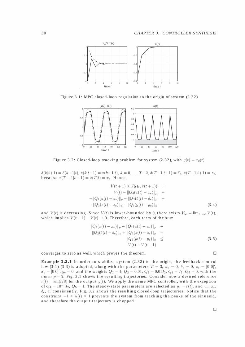
Figure 3.1: MPC closed-loop regulation to the origin of system (2.32)
0 20 40 60 80 100 120-1
-0.5
0
0.5
1
u t( )
time ttime t
y t r t( ), ( )
0 20 40 60 80 100 120
-1
-0.8
-0.6
-0.4
-0.2
0
0.2
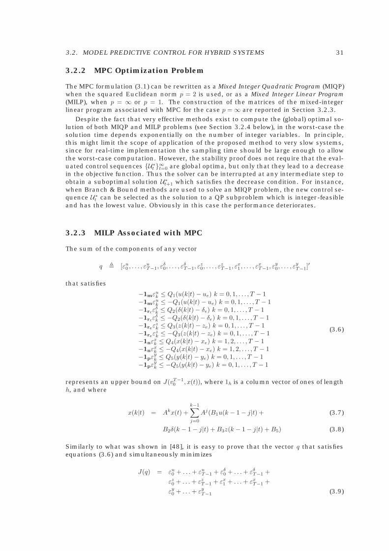
Figure 3.2: Closed-loop tracking problem for system (2.32), with y(t) = x2(t)
δ(k|t+1) = δ(k+1|t), z(k|t+1) = z(k+1|t), k = 0, . . . , T−2, δ(T−1|t+1) = δe, z(T−1|t+1) = ze,because x(T − 1|t+ 1) = x(T |t) = xe. Hence,
V (t+ 1) ≤ J(U1, x(t+ 1)) =V (t)− ‖Q4(x(t) − xe)‖p +
−‖Q1(u(t)− ue)‖p − ‖Q2(δ(t)− δe)‖p +−‖Q3(z(t)− ze)‖p − ‖Q5(y(t)− ye)‖p (3.4)
and V (t) is decreasing. Since V (t) is lower-bounded by 0, there exists V∞ = limt→∞ V (t),which implies V (t+ 1)− V (t)→ 0. Therefore, each term of the sum
‖Q4(x(t)− xe)‖p + ‖Q1(u(t)− ue)‖p +‖Q2(δ(t)− δe)‖p + ‖Q3(z(t)− ze)‖p +
‖Q5(y(t)− ye)‖p ≤ (3.5)
V (t)− V (t+ 1)
converges to zero as well, which proves the theorem. �
Example 3.2.1 In order to stabilize system (2.32) to the origin, the feedback controllaw (3.1)–(3.3) is adopted, along with the parameters T = 3, ue = 0, δe = 0, ze = [0 0]′,xe = [0 0]′, ye = 0, and the weights Q1 = 1, Q2 = 0.01, Q3 = 0.01I2, Q4 = I2, Q5 = 0, with thenorm p = 2. Fig. 3.1 shows the resulting trajectories. Consider now a desired referencer(t) = sin(t/8) for the output y(t). We apply the same MPC controller, with the exceptionof Q4 = 10−8I2, Q5 = 1. The steady-state parameters are selected as ye = r(t), and ue, xe,δe, ze consistently. Fig. 3.2 shows the resulting closed-loop trajectories. Notice that theconstraint −1 ≤ u(t) ≤ 1 prevents the system from tracking the peaks of the sinusoid,and therefore the output trajectory is chopped.
�
3.2. MODEL PREDICTIVE CONTROL FOR HYBRID SYSTEMS 31
3.2.2 MPC Optimization Problem
The MPC formulation (3.1) can be rewritten as a Mixed Integer Quadratic Program (MIQP)when the squared Euclidean norm p = 2 is used, or as a Mixed Integer Linear Program(MILP), when p = ∞ or p = 1. The construction of the matrices of the mixed-integerlinear program associated with MPC for the case p =∞ are reported in Section 3.2.3.
Despite the fact that very effective methods exist to compute the (global) optimal so-lution of both MIQP and MILP problems (see Section 3.2.4 below), in the worst-case thesolution time depends exponentially on the number of integer variables. In principle,this might limit the scope of application of the proposed method to very slow systems,since for real-time implementation the sampling time should be large enough to allowthe worst-case computation. However, the stability proof does not require that the eval-uated control sequences {U∗
t }∞t=0 are global optima, but only that they lead to a decreasein the objective function. Thus the solver can be interrupted at any intermediate step toobtain a suboptimal solution U∗
t+1 which satisfies the decrease condition. For instance,when Branch & Bound methods are used to solve an MIQP problem, the new control se-quence U∗
t can be selected as the solution to a QP subproblem which is integer-feasibleand has the lowest value. Obviously in this case the performance deteriorates.
3.2.3 MILP Associated with MPC
The sum of the components of any vector
q � [εu0 , . . . , ε
uT−1, ε
δ0, . . . , ε
δT−1, ε
z0, . . . , ε
zT−1, ε
x1 , . . . , ε
xT−1, ε
y0, . . . , ε
yT−1]
′
that satisfies
−1mεuk ≤ Q1(u(k|t)− ue) k = 0, 1, . . . , T − 1
−1mεuk ≤ −Q1(u(k|t)− ue) k = 0, 1, . . . , T − 1
−1r�εδ
k ≤ Q2(δ(k|t)− δe) k = 0, 1, . . . , T − 1−1r�
εδk ≤ −Q2(δ(k|t)− δe) k = 0, 1, . . . , T − 1
−1rcεzk ≤ Q3(z(k|t)− ze) k = 0, 1, . . . , T − 1
−1rcεzk ≤ −Q3(z(k|t)− ze) k = 0, 1, . . . , T − 1
−1nεxk ≤ Q4(x(k|t) − xe) k = 1, 2, . . . , T − 1
−1nεxk ≤ −Q4(x(k|t)− xe) k = 1, 2, . . . , T − 1
−1pεyk ≤ Q5(y(k|t)− ye) k = 0, 1, . . . , T − 1
−1pεyk ≤ −Q5(y(k|t)− ye) k = 0, 1, . . . , T − 1
(3.6)
represents an upper bound on J(vT−10 , x(t)), where 1h is a column vector of ones of length
h, and where
x(k|t) = Akx(t) +k−1∑j=0
Aj(B1u(k − 1− j|t) + (3.7)
B2δ(k − 1− j|t) +B3z(k − 1− j|t) +B5) (3.8)
Similarly to what was shown in [48], it is easy to prove that the vector q that satisfiesequations (3.6) and simultaneously minimizes
J(q) = εu0 + . . .+ εu
T−1 + εδ0 + . . .+ εδ
T−1 +εz0 + . . .+ εz
T−1 + εx1 + . . .+ εx
T−1 +εy0 + . . .+ εy
T−1 (3.9)
32 CHAPTER 3. CONTROLLER SYNTHESIS
also solves the original problem, i.e. the same optimum J∗(vT−10 , x(t)) is achieved. There-
fore, problem (3.1) can be reformulated as the following MILP problem
minq
J(q) = [1 1 . . . 1]q
s.t. −1mεuk ≤ ±Q1(u(k|t)− ue), k = 0, 1, . . . , T − 1
−1mεδk ≤ ±Q2(δ(k|t)− δe), k = 0, 1, . . . , T − 1
−1mεzk ≤ ±Q3(z(k|t)− ze), k = 0, 1, . . . , T − 1
−1nεxk ≤ ±Q4(Akx(0|t) +
∑k−1j=0 A
j(B1v(u − 1− j|t)+B2δ(k − 1− j|t) +B3u(k − 1− j|t))− xe), k = 1, . . . , T − 1
−1nεyk ≤ ±Q5(CAkx(0|t) + C
∑k−1j=0 A
j(B1u(k − 1− j|t)+B2δ(k − 1− j|t) +B3z(k − 1− j|t)))+D1u(k) +D2δ(k|t) +D3z(k|t)− ye), k = 0, . . . , T − 1
xmin ≤ Akx(0|t) +∑k−1
j=0 Aj(B1u(k − 1− j|t)+
B2δ(k − 1− j|t) +B3z(k − 1− j|t)) ≤ xmax, k = 1, . . . , Tumin ≤ u(k|t) ≤ umax, k = 0, 1, . . . , T − 1
x(T |t) = xe
x(k + 1|t) = Ax(k|t) +B1u(k) +B2δ(k|t) +B3z(k|t), k ≥ 0y(k|t) = Cx(k|t) +D1u(k) +D2δ(k|t) +D3z(k|t)
E2δ(k|t) + E3z(k|t) ≤ E1u(k) + E4x(k|t) + E5 k ≥ 0E2δ(k|t) + E3z(k|t) = E1u(k) + E4x(k|t) + E5, k ≥ 0
(3.10)
where the variable x(0|t) appears only in the constraints in (3.10) as a vector parameter.Problem (3.10) can be rewritten in the more compact MILP form
q∗t � argminq
fTc qc + fT
d qd
s.t. Gcqc +Gcqd ≤ S + Fx(t)(3.11)
where the matrices G, S, F can be straightforwardly defined from (3.10), and qc, qd rep-resent the continuous and binary components, respectively, of the optimization vector q.The case of quadratic cost functions leads to an MIQP, whose derivation is very similarand therefore omitted here.
3.2.4 Mixed Integer Program Solvers
With the exception of particular structures, mixed-integer programming problems in-volving 0-1 variables are classified as NP -complete, which means that in the worst case,the solution time grows exponentially with the problem size [119]. Despite this combina-torial nature, several packages exist for solving MILP and MIQP problems, including thecommercial software Cplex [92], and other software packages [61,75,104,125]. A basicMILP/MIQP solver implemented in Matlab is also freely available for download [29].
Many algorithmic approaches have been proposed and applied successfully to mediumand large size application problems [76], the four major ones being
• Cutting plane methods, where new constraints (or “cuts”) are generated and addedto reduce the feasible domain until a 0-1 optimal solution is found.
• Decomposition methods, where the mathematical structure of the models is ex-ploited via variable partitioning, duality, and relaxation methods.
• Logic-based methods, where disjunctive constraints or symbolic inference tech-niques are utilized which can be expressed in terms of binary variables.
3.3. EXPLICIT HYBRID MPC CONTROL LAWS 33
• Branch and Bound / Branch and Cut methods, where the 0-1 combinations areexplored through a binary tree, the feasible region is partitioned into sub-domainssystematically, and valid upper and lower bounds are generated at different levelsof the binary tree.
See [124] for a review of these methods. For MIQP, in [75] a numerical study comparesthe different approaches, and Branch and Bound is shown to be superior by an order ofmagnitude. While OA and GBD techniques can be attractive for general Mixed-IntegerNonlinear Problems (MINLP), for MIQP at each node the relaxed QP problem can besolved without approximations and reasonably quickly (for instance, the Hessian matrixof each relaxed QP is constant).
As described by [75], the Branch and Bound algorithm for MIQP consists of solvingand generating new QP problems in accordance with a tree search, where the nodesof the tree correspond to QP subproblems. Branching is obtained by generating child-nodes from parent-nodes according to branching rules, which can be based for instanceon a-priori specified priorities on integer variables, or on the amount by which the inte-ger constraints are violated. Nodes are labeled as either pending, if the correspondingQP problem has not yet been solved, or fathomed, if the node has already been fullyexplored. The algorithm stops when all nodes have been fathomed. The success of thebranch and bound algorithm relies on the fact that whole subtrees can be excluded fromfurther exploration by fathoming the corresponding root nodes. This happens if the cor-responding QP subproblem is either infeasible or an integer solution is obtained. In thesecond case, the corresponding value of the cost function serves as an upper bound onthe optimal solution of the MIQP problem, and is used to further fathoming other nodeshaving greater optimal value or lower bound.
The simulation results reported here have been obtained by interfacing Matlab withthe mixed-integer solvers [29, 61, 92, 104, 125]. All these have different advantages, interms of reliability, speed, platform portability, etc.
3.3 Explicit Hybrid MPC Control Laws
There is an alternative to on-line mixed integer optimization for implementing MPC forhybrid systems.
By generalizing the result of [33] for linear systems to hybrid systems, we proposedthe idea in [15, 16] of handling the state vector x(t), which appears in the the linearpart of the objective function and of the rhs of the constraints, as a vector of param-eters. Then, for performance indices based on the ∞-norm, the optimization problemcan be treated as a multi-parametric MILP (mp-MILP). Solving an mp-MILP amounts toexpress the solution of the MILP as a function of the parameters, as we will detail inSection 3.3.1.
Once the multi-parametric problem (3.1) has been solved off line, i.e., the solutionU∗
t = f(x(t)) of (3.1) has been found, the model predictive controller is available explicitly.In [1] the authors also show that the solution U∗ = f(x) of the mp-MILP problem ispiecewise affine. Clearly, the same properties are inherited by the controller, i.e.,
u(t) = Fix(t) + gi, forx(t) ∈ Xi � {x : Hix ≤ Si}, i = 1, . . . , s
(3.12)
where ∪si=1Xi is the set of states for which a feasible solution to (3.1) exists.
We remark that the piecewise affine controller (3.12) and the MPC controller (3.1) areequal, in the sense that they produce the same control action, and therefore share thesame stabilizing and optimality properties. The difference is only in the implementation:for the form (3.12), on-line computation reduces to a function evaluation, instead of anexpensive mixed-integer linear program.
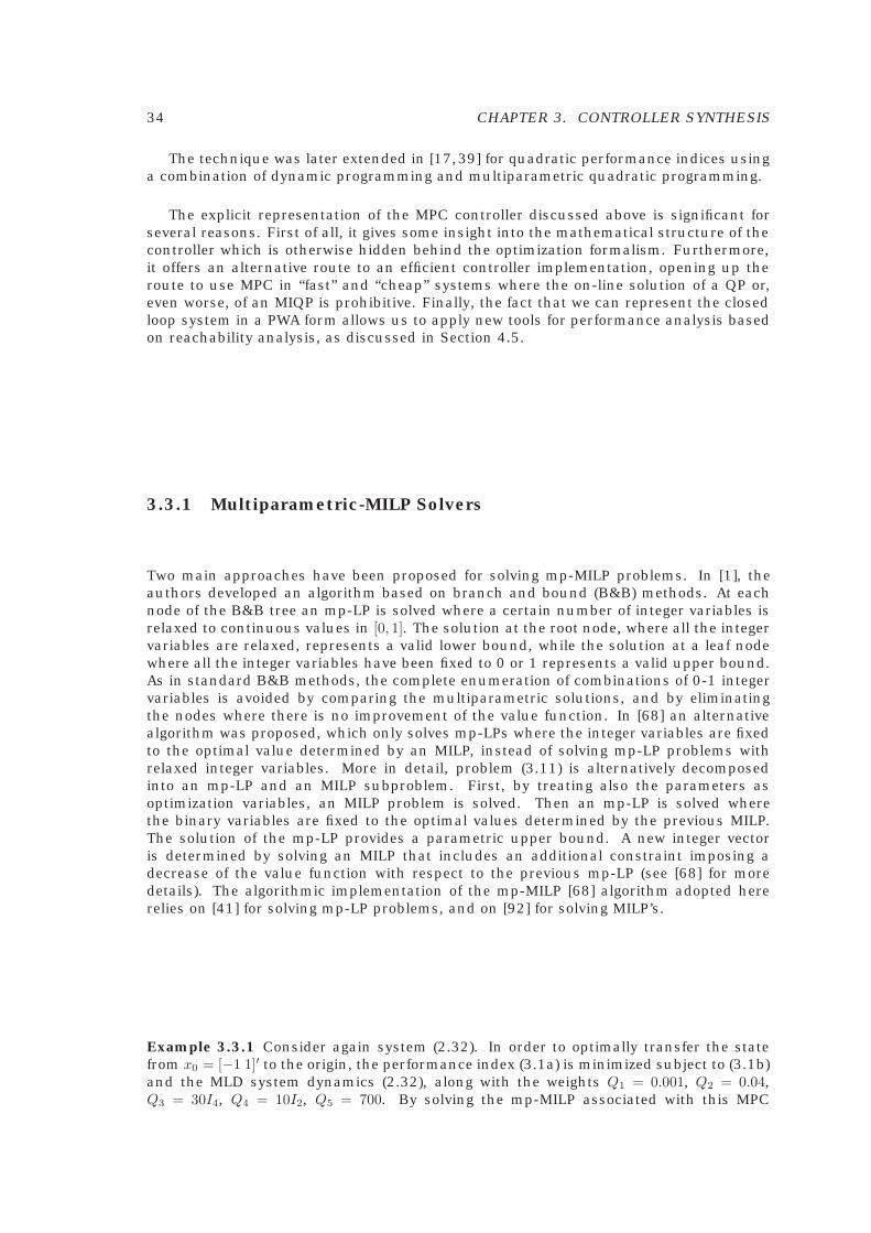
34 CHAPTER 3. CONTROLLER SYNTHESIS
The technique was later extended in [17,39] for quadratic performance indices usinga combination of dynamic programming and multiparametric quadratic programming.
The explicit representation of the MPC controller discussed above is significant forseveral reasons. First of all, it gives some insight into the mathematical structure of thecontroller which is otherwise hidden behind the optimization formalism. Furthermore,it offers an alternative route to an efficient controller implementation, opening up theroute to use MPC in “fast” and “cheap” systems where the on-line solution of a QP or,even worse, of an MIQP is prohibitive. Finally, the fact that we can represent the closedloop system in a PWA form allows us to apply new tools for performance analysis basedon reachability analysis, as discussed in Section 4.5.
3.3.1 Multiparametric-MILP Solvers
Two main approaches have been proposed for solving mp-MILP problems. In [1], theauthors developed an algorithm based on branch and bound (B&B) methods. At eachnode of the B&B tree an mp-LP is solved where a certain number of integer variables isrelaxed to continuous values in [0, 1]. The solution at the root node, where all the integervariables are relaxed, represents a valid lower bound, while the solution at a leaf nodewhere all the integer variables have been fixed to 0 or 1 represents a valid upper bound.As in standard B&B methods, the complete enumeration of combinations of 0-1 integervariables is avoided by comparing the multiparametric solutions, and by eliminatingthe nodes where there is no improvement of the value function. In [68] an alternativealgorithm was proposed, which only solves mp-LPs where the integer variables are fixedto the optimal value determined by an MILP, instead of solving mp-LP problems withrelaxed integer variables. More in detail, problem (3.11) is alternatively decomposedinto an mp-LP and an MILP subproblem. First, by treating also the parameters asoptimization variables, an MILP problem is solved. Then an mp-LP is solved wherethe binary variables are fixed to the optimal values determined by the previous MILP.The solution of the mp-LP provides a parametric upper bound. A new integer vectoris determined by solving an MILP that includes an additional constraint imposing adecrease of the value function with respect to the previous mp-LP (see [68] for moredetails). The algorithmic implementation of the mp-MILP [68] algorithm adopted hererelies on [41] for solving mp-LP problems, and on [92] for solving MILP’s.
Example 3.3.1 Consider again system (2.32). In order to optimally transfer the statefrom x0 = [−1 1]′ to the origin, the performance index (3.1a) is minimized subject to (3.1b)and the MLD system dynamics (2.32), along with the weights Q1 = 0.001, Q2 = 0.04,Q3 = 30I4, Q4 = 10I2, Q5 = 700. By solving the mp-MILP associated with this MPC
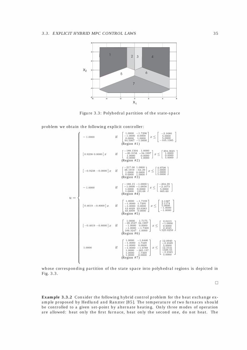
3.3. EXPLICIT HYBRID MPC CONTROL LAWS 35
X1
X2
12 3 4
5 6
7
Figure 3.3: Polyhedral partition of the state-space
problem we obtain the following explicit controller:
u =
− 1.0000 if
[1.0000 −1.7296−1.0000 0.00000.0000 1.000094.5067 −1.0000
]x ≤
[ −2.16805.00005.0000
−105.1385
]
(Region #1)
[ 0.9238 0.0000 ] x if[−188.1504 1.0000
−20.3158 −34.19971.0000 0.00000.0000 1.0000
]x ≤
[204.36211.00000.00005.0000
](Region #2)
[−0.9238 −0.0000 ] x if[−217.00 1.0000
38.1919 −64.291.0000 0.00000.0000 1.0000
]x ≤
[4.97081.00001.00005.0000
](Region #3)
− 1.0000 if[−188.15 −1.0000−1.0000 −1.68581.0000 0.00001.0000 133.68
]x ≤
[−204.39−2.16735.0000665.60
](Region #4)
[ 0.4619 −0.8000 ] x if
1.0000 −1.7193
−1.0000 1.7295−1.0000 0.000013.4029 23.638343.4009 0.0000
x ≤
2.1387
2.11745.0000−1.0000−1.0000
(Region #5)
[−0.4619 −0.8000 ] x if
1.0000 1.7175
−20.2527 34.1997−1.0000 0.0000−1.0000 −1.7369106.3247 1.0000
x ≤
[ 2.0413−1.00000.00002.2345
525.0259
]
(Region #6)
1.0000 if
1.0000 −1.6446−1.0000 1.7449−1.0000 0.0000−1.0000 −1.67881.0000 −265.1371.0000 1.73691.0000 0.0000
x ≤
12.0940−2.24485.000012.31411329.55−2.23455.0000
(Region #7)
whose corresponding partition of the state space into polyhedral regions is depicted inFig. 3.3.
�
Example 3.3.2 Consider the following hybrid control problem for the heat exchange ex-ample proposed by Hedlund and Ranzter [85]. The temperature of two furnaces shouldbe controlled to a given set-point by alternate heating. Only three modes of operationare allowed: heat only the first furnace, heat only the second one, do not heat. The
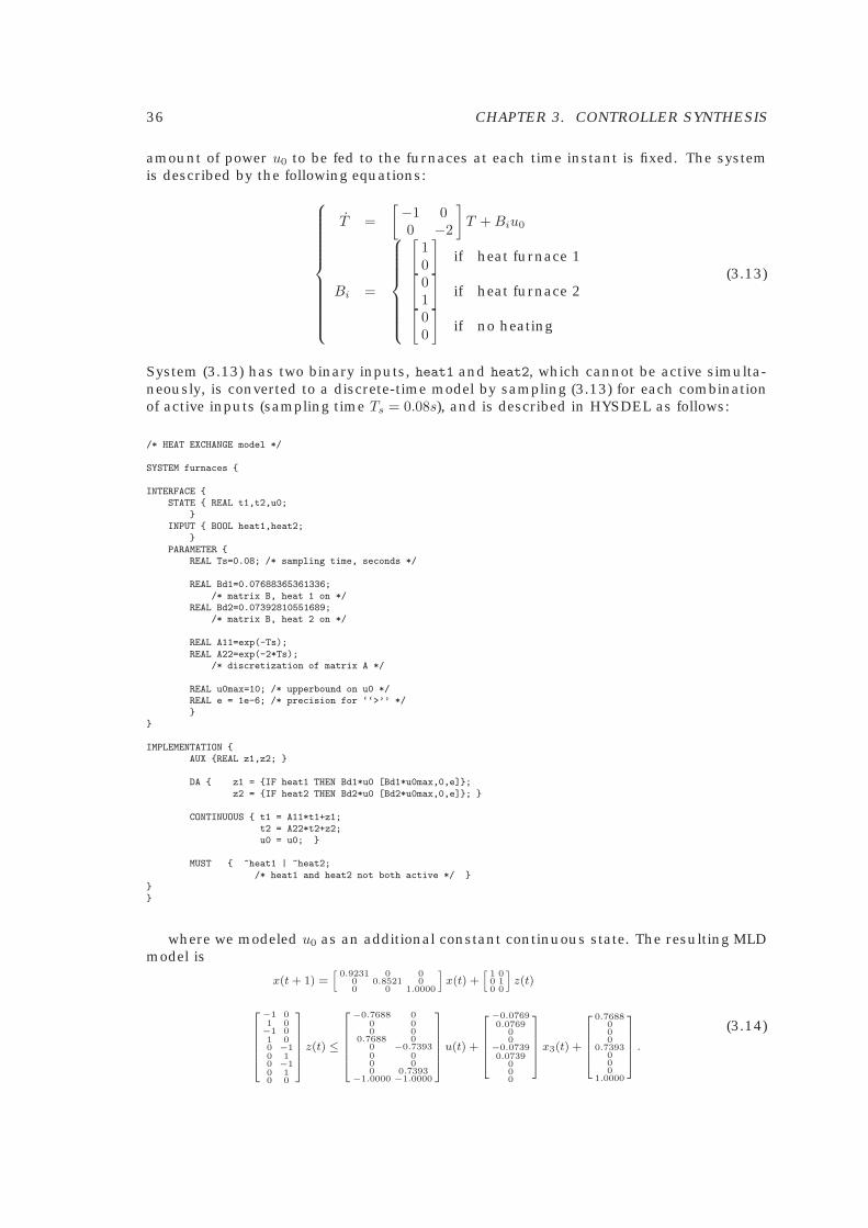
36 CHAPTER 3. CONTROLLER SYNTHESIS
amount of power u0 to be fed to the furnaces at each time instant is fixed. The systemis described by the following equations:
T =[−1 00 −2
]T +Biu0
Bi =
[10
]if heat furnace 1[
01
]if heat furnace 2[
00
]if no heating
(3.13)
System (3.13) has two binary inputs, heat1 and heat2, which cannot be active simulta-neously, is converted to a discrete-time model by sampling (3.13) for each combinationof active inputs (sampling time Ts = 0.08s), and is described in HYSDEL as follows:
/* HEAT EXCHANGE model */
SYSTEM furnaces {
INTERFACE {STATE { REAL t1,t2,u0;
}INPUT { BOOL heat1,heat2;
}PARAMETER {
REAL Ts=0.08; /* sampling time, seconds */
REAL Bd1=0.07688365361336;/* matrix B, heat 1 on */
REAL Bd2=0.07392810551689;/* matrix B, heat 2 on */
REAL A11=exp(-Ts);REAL A22=exp(-2*Ts);
/* discretization of matrix A */
REAL u0max=10; /* upperbound on u0 */REAL e = 1e-6; /* precision for ‘‘>’’ */}
}
IMPLEMENTATION {AUX {REAL z1,z2; }
DA { z1 = {IF heat1 THEN Bd1*u0 [Bd1*u0max,0,e]};z2 = {IF heat2 THEN Bd2*u0 [Bd2*u0max,0,e]}; }
CONTINUOUS { t1 = A11*t1+z1;t2 = A22*t2+z2;u0 = u0; }
MUST { ~heat1 | ~heat2;/* heat1 and heat2 not both active */ }
}}
where we modeled u0 as an additional constant continuous state. The resulting MLDmodel is
x(t+ 1) =[
0.9231 0 00 0.8521 00 0 1.0000
]x(t) +
[1 00 10 0
]z(t)
−1 01 0−1 01 00 −10 10 −10 10 0
z(t) ≤
−0.7688 00 00 0
0.7688 00 −0.73930 00 00 0.7393
−1.0000 −1.0000
u(t) +
−0.07690.0769
00
−0.07390.0739
000
x3(t) +
0.7688000
0.7393000
1.0000
.
(3.14)
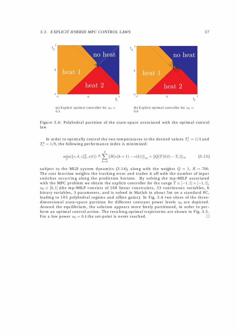
3.3. EXPLICIT HYBRID MPC CONTROL LAWS 37
-1 0 1
-1
0
1
T2
T1
no heat
heat 1
heat 2
(a) Explicit optimal controller for u0 =0.4
T1
T2
-1 0 1-1
0
1
no heat
heat 1
heat 2
(b) Explicit optimal controller for u0 =0.8
Figure 3.4: Polyhedral partition of the state-space associated with the optimal controllaw
In order to optimally control the two temperatures to the desired values T 1e = 1/4 and
T 2e = 1/8, the following performance index is minimized:
minJ
({v, δ, z}20, x(t)) �2∑
k=0
‖R(v(k + 1)− v(k))‖∞ + ‖Q(T (k|t)− Te)‖∞ (3.15)
subject to the MLD system dynamics (3.14), along with the weights Q = 1, R = 700.The cost function weights the tracking error and trades it off with the number of inputswitches occurring along the prediction horizon. By solving the mp-MILP associatedwith the MPC problem we obtain the explicit controller for the range T ∈ [−1, 1]× [−1, 1],u0 ∈ [0, 1] (the mp-MILP consists of 168 linear constraints, 33 continuous variables, 6binary variables, 3 parameters, and is solved in Matlab in about 5m on a standard PC,leading to 105 polyhedral regions and affine gains). In Fig. 3.4 two slices of the three-dimensional state-space partition for different constant power levels u0 are depicted.Around the equilibrium, the solution appears more finely partitioned, in order to per-form an optimal control action. The resulting optimal trajectories are shown in Fig. 3.5.For a low power u0 = 0.4 the set-point is never reached. �
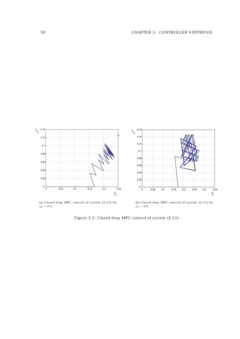
38 CHAPTER 3. CONTROLLER SYNTHESIS
0 0.05 0.1 0.15 0.2 0.25
0
0.02
0.04
0.06
0.08
0.1
0.12
0.14
T1
T2
(a) Closed-loop MPC control of system (3.13) foru0 = 0.4
T2
0 0.05 0.1 0.15 0.2 0.25 0.3 0.35
0
0.02
0.04
0.06
0.08
0.1
0.12
0.14
0.16
T1
(b) Closed-loop MPC control of system (3.13) foru0 = 0.8
Figure 3.5: Closed-loop MPC control of system (3.13)
Chapter 4
Reachability Analysis
Models are mathematical objects that allow one to reproduce the dynamic evolution ofreal plants and to quantitatively analyze their properties. A good model should combinea satisfactory detail of the real system with a tractable mathematical structure in orderto formulate and efficiently solve interesting applicative problems like definition andcomputation of trajectories, stability and safety analysis, control, state estimation, etc.As mentioned in Chapter 1, several classes of hybrid models have been proposed in theliterature, each class is usually tailored to solve a particular problem or it is specific toa certain subclass of hybrid processes, and often can approximate other classes witharbitrary precision, or be equivalent under certain transformations.
A simulation of the mathematical model enables to probe the system, but very oftenit does not permit to assess its structural properties. In fact, any analysis based onsimulation is likely to miss the subtle phenomena that a model may generate, especiallyin the case of hybrid models. Tools like reachability analysis and piecewise quadraticLyapunov stability are becoming a standard in analysis of hybrid systems. Reachabilityanalysis (or safety analysis or formal verification) aims at detecting if a hybrid model willeventually reach an unsafe state configuration or satisfy a temporal logic formula [58].Reachability analysis relies on a reach set computation algorithm, which strongly de-pends on to the mathematical model of the system [127]. Piecewise quadratic Lyapunovstability is a deductive way to prove the stability of an equilibrium point of a subclass ofhybrid systems (piecewise linear systems), the computational burden is usually low, atthe price of a convex relaxation of the problem which may lead to conservative results.
Timed automata and hybrid automata have proved to be a successful modelingframework for formal verification, and have been widely used in the literature. Thestarting point for both models is a finite state machine equipped with continuous dy-namics. In the theory of timed automata [7], the dynamic part is the continuous-timeflow x = c ∈ R
d. Efficient computational tools complete the theory of timed automata andallow one to perform verification [38] and optimal control [11] of such models. Timed au-tomata were extended to linear hybrid automata [3], where the dynamics is modeled bythe differential inclusion a ≤ x ≤ b. Specific tools consent the formal verification of suchmodels against safety and liveness requirements. Linear hybrid automata were furtherextended to hybrid automata where the continuous dynamics is governed by differentialequations. Tools exists to model and analyze those systems, either directly [6,57] or byapproximating the model with timed automata or linear hybrid automata.
In this chapter we present an algorithm that computes the set of states that a givenDHA system can reach within Kmax sampling times from any initial state x(0) ∈ X (0) andunder any possible input excitation of u(t) ∈ U , t = 0, . . . ,Kmax.
By exploiting the linearity of the dynamics in each operating mode of the DHA sys-tem, the proposed reachability algorithm computes the reach set via simple polyhedralcomputations, and using the properties of the Minkowski’s sum it is able to detect the
39
40 CHAPTER 4. REACHABILITY ANALYSIS
set of the state trajectories that have switched mode. A significantly fast analysis isobtained by over-approximating the reach set. This introduces some conservativenessthat is eventually removed in a simple post-processing operation.
The importance of reach set computations is twofold. First, as shown in Section 4.4,it allows one to check for safety/liveness properties, for instance that the trajectories ofthe hybrid system will never enter some unsafe regions of the state space, or that all thetrajectories will reach a target region within a given maximum time. Interesting control-theoretical questions like stability [35] and observability [18] can be reformulated asreachability questions. Second, the proposed algorithmic ingredients for reachabilityanalysis can be suitably used for optimal control purposes: as shown in Section 4.6,if an optimization stage is performed in parallel with reach-set computation, the lattercan be selectively carried out according to a convenient strategy that discards evolutionswhich are recognized not to be optimal, and finally determines the desired optimal inputsequence. Compared with approaches based on mixed-integer programming [31], wherethe complexity depends exponentially on the prediction horizon Kmax, the method pro-posed here appears particularly attractive for solving hybrid optimal/receding horizoncontrol problems where the prediction horizon is large and switching is not frequent.In particular, the larger the number of sampling steps between switches (e.g., becauseof a small sampling time), the more efficient the algorithm is with respect to the useof mixed-integer solvers. An additional feature of this approach is that it intrinsicallyembeds a practical reachability test for the system to be controlled, which is generally aprerequisite.
This chapter summarizes the results in [26, 32, 35, 37] and is mainly based on thereport [132].
4.1 Preliminaries on Polyhedral Computation
The purpose of this section is to recall some basic notions and theorems on convexpolyhedra that will be used later.
For two subsets P1 and P2 of Rd, their Minkowski’s sum, denoted by P1 + P2, is the
set {x : x = x1 + x2, x1 ∈ P1, x2 ∈ P2}. For a finite subset V = {v1, . . . , vn} of Rd, its convex
hull conv(V ) and the conic hull cone(V ) are defined by
conv(V ) := {x : x =n∑
i=1
λivi, λ ≥ 0,n1∑i=1
λi = 1}
cone(V ) := {x : x =n∑
i=1
λivi, λ ≥ 0}.
Here is a fundamental theorem of convex polyhedra.
Theorem 3 (Motzkin’s Theorem [141, p. 30]) For a subset P ⊆ Rd, the following two
statements are equivalent:
(a) P = conv(V ) + cone(R) for some finite subsets V and R of Rd;
(b) P = {x : Ax ≤ B} for some matrix A ∈ Rm×d and some vector B ∈ R
m.
A subset P of Rd represented by either (a) or (b) is called a convex polyhedron or sim-
ply polyhedron. A convex polytope or simply polytope is a bounded convex polyhedron. Arepresentation (V,R) of a convex polyhedron P is called a V-representation, and a repre-sentation (A,B) is an H-representation. A convex polyhedron given by V-representation(H-representation) is called V-polyhedron (H-polyhedron). It is possible to go from onerepresentation to another [77], but the numerical sensitivity and complexity of thoseoperations increases with the dimension d of the polytopes [8].
4.1. PRELIMINARIES ON POLYHEDRAL COMPUTATION 41
Given an H-polyhedron P = {x : Ax ≤ B}, the i-th inequality Aix ≤ Bi is redundantfor P if its removal preserves the polyhedron, i.e. P = {x : Ax ≤ B} = {x : Ajx ≤Bi for all j �= i}. Similarly, given a collection of n points V in R
d, we say that v ∈ V isredundant for V if conv(V ) = conv(V \ {v}).
For two V-polytopes P1 = conv(V ), V = {v1, . . . , vn} and P2 = conv(W ),W = {w1, . . . , wm},the Minkowski’s sum P1 + P2 = conv(Z), Z = {vi + wj , ∀i = 1, . . . , n, ∀j = 1, . . . ,m}, wherehowever many of the vertices in Z might be redundant. It is possible to compute aV-representation of P1 + P2 minimal in the number of vertices [78,84,113].
Given two H-polytopes P1 = {x : A1x ≤ B1} and P2 = {x : A2 ≤ B2}, the Minkowski’ssum P1 + P2 = {x : x = x1 + x2, A1x1 ≤ B1, A2x2 ≤ B2}. It is possible to eliminate the vari-ables x1 and x2 from the definition of P1+P2 by using Fourier-Motzkin elimination [141],however, in general, the Fourier-Motzkin elimination provides an highly redundant H-representation.
Remark 4.1.1 It follows from the definition of Minkowski’s sum that the maximum ofa linear function fx on P1 + P2 is the sum of the maxima on the single polytopes, i.e.:maxx∈(P1+P2) fx = maxx∈P1 fx + maxx∈P2 fx, and argmaxx∈(P1+P2) fx = arg maxx∈P1 fx +arg maxx∈P2 fx.
�The problem of determining if a polytope P is contained in a polytope Q is known
as a containment problem in the field of computational convexity. If P is a V-polytopeand Q is given in H-representation, then the solution is trivial. If P and Q are both V-or H-polytopes then the problem has a polynomial-time solution. Finally if P is givenin H-representation and Q is a V-polytope then problem is coNP-complete [83, Theorem4.1].
The following Lemma allows one to check if the Minkowski’s sum of polytopes iscontained in a given H-polytope.
Lemma 3 Given n polytopes P1, P2, . . . , Pn and a H-polytope Q = {x : Ax ≤ B}, letAjx ≤ Bj , j ∈ J = {1, . . . ,m} be the j-th inequality of Q. (P1 +P2 + . . .+Pn) ⊆ Q, if and onlyif∑n
i=1(maxx∈Pi Ajx) ≤ Bj , ∀j ∈ J .
Proof. Denote by Ps the Minkowski’s sum (P1+P2+ . . .+Pn). We first prove the “if” part ofthe lemma. By Remark 4.1.1, the point x =
∑ni=1 arg maxx∈Pi Ajx = arg maxx∈Ps Ajx is the
point that maximizes the normal to the j-th constraint of Q on the set Ps. If Aj x ≤ Bj
then Ajx ≤ Bj for all the x ∈ Ps, i.e. all the points of Ps satisfy the j-th constraintof Q. As this holds for all j ∈ J then Ps ⊆ Q. For proving the “only if” part, assumeby contradiction that there exists some such that
∑ni=1(maxx∈Pi Ax) > B. Then, the
point x =∑n
i=1 argmaxx∈Pi Ax does not satisfy the -th constraint of Q but x ∈ Ps andcontradicts the hypothesis Ps ⊆ Q. �
The weighted Minkowski’s sum of n polytopes P1 ∈ Rd1, P2 ∈ R
d2, . . . , Pn ∈ Rdn with
weights R1 ∈ Rd×d1, R2 ∈ R
d×d2, . . . , Rn ∈ Rd×dn denoted by R1P1 + R2P2 + . . . + RnPn =∑n
i=1RiPi, is defined inductively as:
1. M1 = {x : R1x1, x1 ∈ P1},
2. Mi = Mi−1 +RiPi = {x : x = xi−1 +Rixi, xi ∈Mi−1, xn ∈ Pn}, for i = 2, . . . , n.
The weighted Minkowski’s sum R1P1+R2P2+. . .+RnPn is a polytope as it is the projectionof the polytope P1 × P2 × . . .× Pn on the coordinates x = R1x1 +R2x2 + . . . Rnxn [141].
Remark 4.1.2 It follows directly from the definition that a weighted Minkowski’s sum∑ni=1RiPi is feasible if and only if all the sets Pi are feasible.
�The proof of the following is along the same lines of Lemma 3 and is therefore omitted.
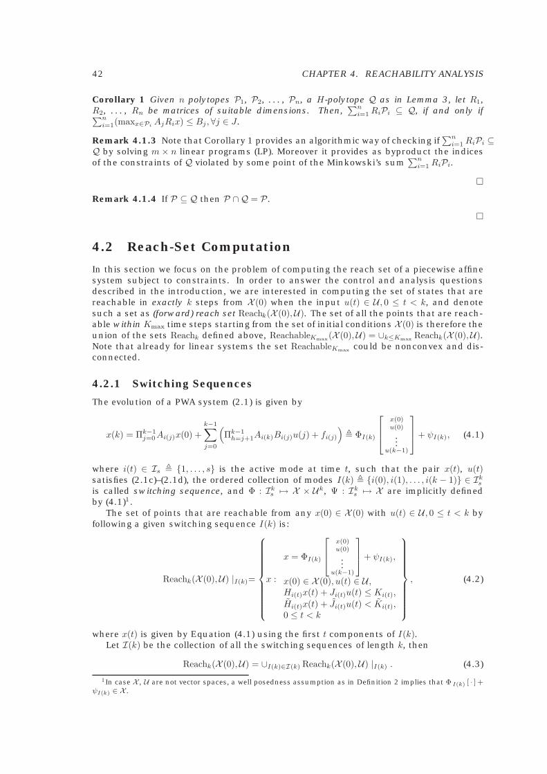
42 CHAPTER 4. REACHABILITY ANALYSIS
Corollary 1 Given n polytopes P1, P2, . . . , Pn, a H-polytope Q as in Lemma 3, let R1,R2, . . . , Rn be matrices of suitable dimensions. Then,
∑ni=1RiPi ⊆ Q, if and only if∑n
i=1(maxx∈Pi AjRix) ≤ Bj , ∀j ∈ J .
Remark 4.1.3 Note that Corollary 1 provides an algorithmic way of checking if∑n
i=1 RiPi ⊆Q by solving m × n linear programs (LP). Moreover it provides as byproduct the indicesof the constraints of Q violated by some point of the Minkowski’s sum
∑ni=1 RiPi.
�
Remark 4.1.4 If P ⊆ Q then P ∩Q = P.
�
4.2 Reach-Set Computation
In this section we focus on the problem of computing the reach set of a piecewise affinesystem subject to constraints. In order to answer the control and analysis questionsdescribed in the introduction, we are interested in computing the set of states that arereachable in exactly k steps from X (0) when the input u(t) ∈ U , 0 ≤ t < k, and denotesuch a set as (forward) reach set Reachk(X (0),U). The set of all the points that are reach-able within Kmax time steps starting from the set of initial conditions X (0) is therefore theunion of the sets Reachk defined above, ReachableKmax(X (0),U) = ∪k≤Kmax Reachk(X (0),U).Note that already for linear systems the set ReachableKmax could be nonconvex and dis-connected.
4.2.1 Switching Sequences
The evolution of a PWA system (2.1) is given by
x(k) = Πk−1j=0Ai(j)x(0) +
k−1∑j=0
(Πk−1
h=j+1Ai(k)Bi(j)u(j) + fi(j)
)� ΦI(k)
x(0)u(0)
...u(k−1)
+ ψI(k), (4.1)
where i(t) ∈ Is � {1, . . . , s} is the active mode at time t, such that the pair x(t), u(t)satisfies (2.1c)–(2.1d), the ordered collection of modes I(k) � {i(0), i(1), . . . , i(k − 1)} ∈ Ik
s
is called switching sequence, and Φ : Iks → X × Uk, Ψ : Ik
s → X are implicitly definedby (4.1)1.
The set of points that are reachable from any x(0) ∈ X (0) with u(t) ∈ U , 0 ≤ t < k byfollowing a given switching sequence I(k) is:
Reachk(X (0),U) |I(k)=
x :
x = ΦI(k)
x(0)u(0)
...u(k−1)
+ ψI(k),
x(0) ∈ X (0), u(t) ∈ U ,Hi(t)x(t) + Ji(t)u(t) ≤ Ki(t),
Hi(t)x(t) + Ji(t)u(t) < Ki(t),0 ≤ t < k
, (4.2)
where x(t) is given by Equation (4.1) using the first t components of I(k).Let I(k) be the collection of all the switching sequences of length k, then
Reachk(X (0),U) = ∪I(k)∈I(k) Reachk(X (0),U) |I(k) . (4.3)
1In case X , U are not vector spaces, a well posedness assumption as in Definition 2 implies that Φ I(k) [ · ] +ψI(k) ∈ X .
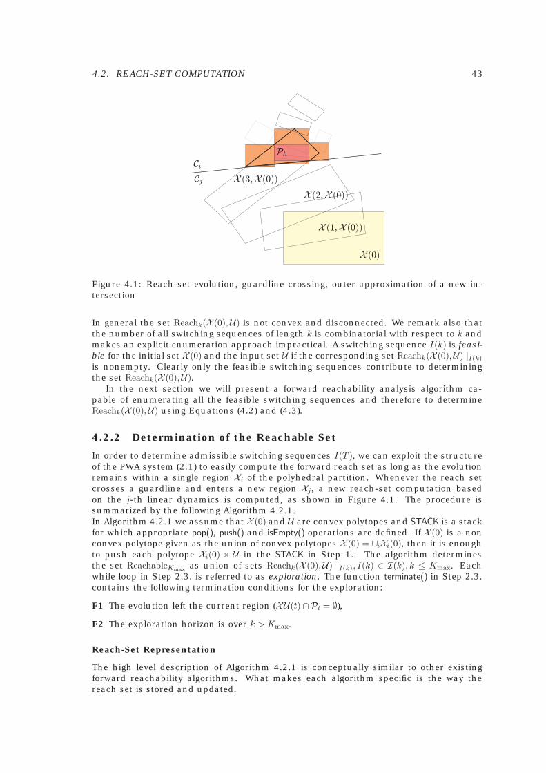
4.2. REACH-SET COMPUTATION 43
Ci
Cj
Ph
X (0)
X (1;X (0))
X (2;X (0))
X (3;X (0))
Figure 4.1: Reach-set evolution, guardline crossing, outer approximation of a new in-tersection
In general the set Reachk(X (0),U) is not convex and disconnected. We remark also thatthe number of all switching sequences of length k is combinatorial with respect to k andmakes an explicit enumeration approach impractical. A switching sequence I(k) is feasi-ble for the initial set X (0) and the input set U if the corresponding set Reachk(X (0),U) |I(k)
is nonempty. Clearly only the feasible switching sequences contribute to determiningthe set Reachk(X (0),U).
In the next section we will present a forward reachability analysis algorithm ca-pable of enumerating all the feasible switching sequences and therefore to determineReachk(X (0),U) using Equations (4.2) and (4.3).
4.2.2 Determination of the Reachable Set
In order to determine admissible switching sequences I(T ), we can exploit the structureof the PWA system (2.1) to easily compute the forward reach set as long as the evolutionremains within a single region Xi of the polyhedral partition. Whenever the reach setcrosses a guardline and enters a new region Xj, a new reach-set computation basedon the j-th linear dynamics is computed, as shown in Figure 4.1. The procedure issummarized by the following Algorithm 4.2.1.In Algorithm 4.2.1 we assume that X (0) and U are convex polytopes and STACK is a stackfor which appropriate pop(), push() and isEmpty() operations are defined. If X (0) is a nonconvex polytope given as the union of convex polytopes X (0) = ∪iXi(0), then it is enoughto push each polytope Xi(0) × U in the STACK in Step 1.. The algorithm determinesthe set ReachableKmax as union of sets Reachk(X (0),U) |I(k), I(k) ∈ I(k), k ≤ Kmax. Eachwhile loop in Step 2.3. is referred to as exploration. The function terminate() in Step 2.3.contains the following termination conditions for the exploration:
F1 The evolution left the current region (XU(t) ∩ Pi = ∅),
F2 The exploration horizon is over k > Kmax.
Reach-Set Representation
The high level description of Algorithm 4.2.1 is conceptually similar to other existingforward reachability algorithms. What makes each algorithm specific is the way thereach set is stored and updated.
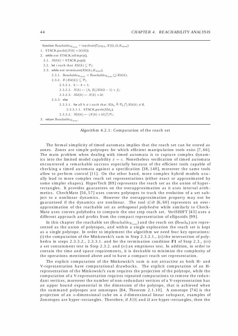
44 CHAPTER 4. REACHABILITY ANALYSIS
function ReachableKmax = reachset(ΣPWA,X (0), U ,Kmax)
1. STACK.push((X (0) × U)(0));
2. while not STACK.isEmpty(),
2.1. XU(k) = STACK.pop();
2.2. let i such that XU(k) ⊆ Pi;
2.3. while not terminate(XU(k),Kmax),
2.3.1. ReachableKmax = ReachableKmax
⋃ XU(k);
2.3.2. if (XU(k)) ⊆ Pi,
2.3.2.1. k ← k + 1;
2.3.2.2. X (k)← [Ai Bi]XU(k − 1) + fi;
2.3.2.3. XU(k)← X (k)× U ;
2.3.3. else
2.3.3.1. for all h �= i such that XUh � Ph⋂XU(k) �= ∅,
2.3.3.1.1. STACK.push(XUh);
2.3.3.2. XU(k)← (X (k)× U)⋂Pi;
3. return ReachableKmax .
Algorithm 4.2.1: Computation of the reach set
The formal simplicity of timed automata implies that the reach set can be stored aszones. Zones are simple polytopes for which efficient manipulation tools exist [7, 66].The main problem when dealing with timed automata is to capture complex dynam-ics into the limited model capability x = c. Nonetheless verification of timed automataencountered a remarkable success especially because of the efficient tools capable ofchecking a timed automata against a specification [38, 140], moreover the same toolsallow to perform control [11]. On the other hand, more complex hybrid models usu-ally lead to more complex reach set representations (either exact or approximated bysome simpler shapes). HyperTech [89] represents the reach set as the union of hyper-rectangles. It provides guarantees on the overapproximation as it uses interval arith-metics. ChechMate [56, 57] uses convex polytopes to track the evolution of a set sub-ject to a nonlinear dynamics. However the overapproximation property may not beguaranteed if the dynamics are nonlinear. The tool d/dt [6, 60] represents an over-approximation of the reachable set as orthogonal polyhedra while similarly to Check-Mate uses convex polyhedra to compute the one step reach set. VeriSHIFT [43] uses adifferent approach and profits from the compact representation of ellipsoids [99].
In this chapter the reachable set (ReachableKmax ) and the reach set (Reachk) are repre-sented as the union of polytopes, and within a single exploration the reach set is keptas a single polytope. In order to implement the algorithm we need four key operations:(i) the computation of the Minkowski’s sum in Step 2.3.2.1., (ii) the intersection of poly-hedra in steps 2.3.3.2., 2.3.3.1. and for the termination condition F1 of Step 2.3., (iii)a set containment test in Step 2.3.2. and (iv) an emptiness test. In addition, in order tocontain the time and space requirements, it is desirable to minimize the complexity ofthe operations mentioned above and to have a compact reach set representation.
The explicit computation of the Minkowski’s sum is not attractive as both H- andV-representation have computational drawbacks. The explicit computation of an H-representation of the Minkowski’s sum requires the projection of the polytope, while thecomputation of a V-representation requires repeated computations to remove the redun-dant vertices, moreover the number of non-redundant vertices of a V-representation hasan upper bound exponential in the dimension of the polytope, that is achieved whenthe summand polytopes are zonotopes [84, Theorem 2.1.10]. A zonotope [74] is theprojection of an n-dimensional cube on a d-dimensional linear subspace, examples ofZonotopes are hyper-rectangles. Therefore, if X (0) and U are hyper-rectangles, then the

4.2. REACH-SET COMPUTATION 45
reach set for a given switching sequence (Reachk(X (0),U) |I(k)) is a zonotope by Equa-tion (4.1). Apart form that, computing the intersection of polytopes in V-representationis the dual problem of the extended convex hull problem, which is computationally in-volving [77].
Each polyhedron is stored as a weighted Minkowski’s sum (we remark once morethat the weighted Minkowski’s sum is an implicit representation where we store thesummand and the weights). It is attractive because it allows to save the operationsneeded for computing the explicit representation and it is compact. Such a representa-tion addresses the first computational request described above.
Example 4.2.1 Consider the reach set of a 4-dimensional linear system with 2 inputson Kmax = 10 steps. Assume that X (0) and U are hyper-rectangles (i.e.: mi ≤ xi ≤ Mi,i = {1, . . . , 4} and nj ≤ uj ≤ Nj, j = {1, 2}) then the number of constraints of X (0) and U isrespectively nx = 8 and nu = 4. The reach set after 10 steps has 4096 vertices, while theimplicit representation would need nx +Kmaxnu = 48 inequalities and Equation (4.1).
�The following Proposition 1 addresses the second computational requirement.
Proposition 1 The intersection of a weighted Minowski’s sum R1P1 +R2P2 + . . .+RnPn,Pi = {x : Cix ≤ Di} with a polytope Q = {x : Ax ≤ B} is a weighted Minkowski’s sum STwhere
S =[R1 R2 . . . Rn
], (4.4)
and
T =
y :
C1 0 · · · 00 C2 · · · 0...
.... . .
...0 0 · · · Cn
AR1 AR2 · · · ARn
y ≤
D1
D2
...Dn
B
. (4.5)
Proof. The set ST is a weighted Minkowski’s sum of one polytope. The first n block ofrows of constraints of T and S are an other way of writing
∑ni=1 RiPi with y = [x′1 . . . x′n]′,
while the last block of constraints of T together with S define the set Q, to see this isenough to substitute x = Sy in the inequalities Ax ≤ B to obtain the last block ofconstraints of T . �
Note that, in general, the H-representation of the set T may contain redundant con-straints. However Corollary 1 and Remark 4.1.3 provide a computational tool to solvethe containment problem and as a byproduct provide the constraints of Q that areviolated by points of the Minkowski’s sum, therefore the intersection of Step 2.3.3.2.contains only non-redundant constraints of Q.
Finally feasibility of a weighted Minkowski’s sum is simply addressed by Remark 4.1.2.We recall here that the feasibility of a H-polytope can be checked by solving a linear pro-gram (LP).
Remark 4.2.1 The containment test in Step 2.3.2. provides information on the con-straints of Pi that are violated. This information can be exploited in the followingStep 2.3.3.1. to save computations and check the intersection only for the regions Ph
that share at least one violated constraint with Pi.
�
Tree of Evolution
The result of the exploration algorithm detailed in the previous sections is convenientlystored in a tree G (see Figure 4.2). The nodes of the tree represent sets from which a

46 CHAPTER 4. REACHABILITY ANALYSIS
XU0
XU1
XU2
1
1
11
1
2 2
22
2
33
44
5
6
k
Figure 4.2: Tree of evolution
reach set evolution is computed, and a branch connects two nodes if a transition existsbetween the two corresponding sets, starting at time k1 and ending at time k2, withi(k) ≡ h, ∀k = k1, . . . , k2, where h ∈ Is is a given mode, associated with the starting node.Each branch b has an associated weight kb = k − 2− k1 which represents the number ofsteps needed for the transition. The root node of the tree is the initial set2 XU0 = X (0)×U ,from which the reach set evolution is computed. When a new set XUh crossing a guard-line is detected, it becomes a new node. The new node is connected by a weightedbranch from XU0, and inserted in a list of sets to be subsequently explored. Then,computation of the reach set proceeds in each region Ph from each new intersectionXUh. The oriented paths on G from the initial node XU0 determine all the feasibleswitching sequences I(Kmax) ∈ IKmax
s .
4.3 Approximate Reachability Analysis
In this section we present tools for determining over-approximations of the reachable setthat have a reduced complexity, in particular that have an associated tree of evolutionwith less nodes. Over-approximations have the consequence of making the analysisconservative when used for instance in the context of verification of safety properties,although, as we will show, this conservativeness can be eventually removed in a simplepost-processing operation.
4.3.1 Approximation of Intersections
The computation of the reach set proceeds in each region Ph from each new intersectionXUh. Before starting a new reach set computation from a set XU j extracted from STACK,we check for inclusion of XUj in other nodes of G. If this happens, say XU j ⊆ XU1 as inFigure 4.3, the node associated with XUj is connected to XU1 with an arc of weight 0.3
2With a slight abuse of notation, XUk will be referred to as both a node of the tree and the associated setin the state space.
3If we are interested in an inner approximation of the reach set then it is enough to direct the new arc inthe other direction.
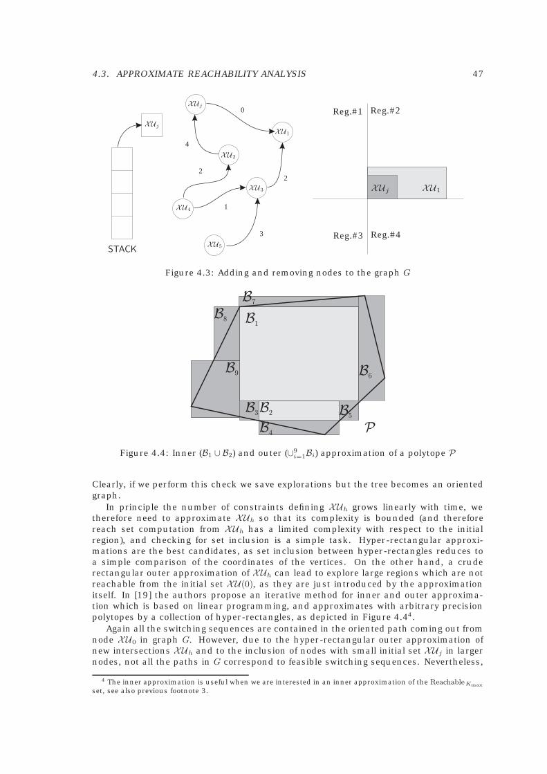
4.3. APPROXIMATE REACHABILITY ANALYSIS 47
0
1
22
3
4
STACK
XUj
XUj
XU1
XU2
XU3
XU4
XU5
Reg.#1 Reg.#2
Reg.#3 Reg.#4
XUj XU1
Figure 4.3: Adding and removing nodes to the graph G
B1
B2
B8
B9
B3
B4
B5
B6
B7
P
Figure 4.4: Inner (B1 ∪ B2) and outer (∪9i=1Bi) approximation of a polytope P
Clearly, if we perform this check we save explorations but the tree becomes an orientedgraph.
In principle the number of constraints defining XUh grows linearly with time, wetherefore need to approximate XUh so that its complexity is bounded (and thereforereach set computation from XUh has a limited complexity with respect to the initialregion), and checking for set inclusion is a simple task. Hyper-rectangular approxi-mations are the best candidates, as set inclusion between hyper-rectangles reduces toa simple comparison of the coordinates of the vertices. On the other hand, a cruderectangular outer approximation of XUh can lead to explore large regions which are notreachable from the initial set XU(0), as they are just introduced by the approximationitself. In [19] the authors propose an iterative method for inner and outer approxima-tion which is based on linear programming, and approximates with arbitrary precisionpolytopes by a collection of hyper-rectangles, as depicted in Figure 4.44.
Again all the switching sequences are contained in the oriented path coming out fromnode XU0 in graph G. However, due to the hyper-rectangular outer approximation ofnew intersections XUh and to the inclusion of nodes with small initial set XUj in largernodes, not all the paths in G correspond to feasible switching sequences. Nevertheless,
4 The inner approximation is useful when we are interested in an inner approximation of the ReachableKmaxset, see also previous footnote 3.

48 CHAPTER 4. REACHABILITY ANALYSIS
Target set Z1
Target set Z2
Initial set XU(0)
XUZ1
XUZ2
Figure 4.5: Verification problem
feasibility of each switching sequence can be simply tested via linear programming5.
4.4 Verification of Safety Properties
The main purpose of reachability analysis is to provide the certification that a givenhybrid dynamical system enjoys certain safety properties, or provide a counterexample.A safety property can be stated as follows: for a given set of initial conditions andexogenous signals, the set of unsafe states is never entered. We formalize the problemof verification of safety properties as follows:
Problem 1 (Verification Problem) Given a hybrid system Σ in PWA form (2.1)6, a set ofinitial conditions X (0), a collection of disjoint target sets Z1, Z2, . . ., ZL, a bounded setof inputs U , and a time interval {0, . . . ,Kmax}, determine (i) if Zj is reachable from X (0)within k ≤ Kmax steps for some sequence {u(0), . . . , u(t − 1)} ⊆ U of exogenous inputs;(ii) if yes, the subset of initial conditions XZj (0) of X (0) from which Zj can be reachedwithin Kmax steps; (iii) for any x1 ∈ XZj (0) and x2 ∈ Zj , (one of) the input sequence(s){u(0), . . . , u(k − 1)} ⊆ U , k ≤ Kmax, that drives x1 to x2.
From now on, we will assume that Zj, are polyhedral sets, and, without loss ofgenerality, that they are also convex. The reason for focusing on finite-time reachabilityis that states which are not reachable in less than Kmax steps are in practice, if Kmax islarge enough, unreachable. Although finite time reachability analysis cannot guaranteecertain liveness properties (for instance, if Zi will be ever reached), the reachabilityproblem stated above is clearly decidable. Nevertheless, the problem is NP -hard [37].
The problem formulated above is very similar to the one stated in [67], where the au-thors use big-M techniques to transform the problem into a mixed integer linear prob-lem (MILP). While here we exploit the reach set computation techniques of Section 4.2,in [67] the solution approach is based on the solution to a (large) MILP that summarizesthe system dynamics over the time Kmax and the target regions configuration. The costfunction aims at maximizing the permanence in the unsafe regions and therefore findsthe less safe trajectory. Although good MILP solvers have a satisfactory performance forlarge problems, the problem might become intractable already for small Kmax.
The previous questions of verification can be answered once all the switching se-quences I(k), ∀k ≤ Kmax leading to Z1, or Z2, . . . , or ZL from XU(0) = X (0) × U aredetermined using Algorithm 4.2.1. In fact, it is enough to check that the reach set attime k satisfies Reachk(X ,U) ∩ Zj �= ∅. Nonetheless Algorithm 4.2.1 can be improved byexploiting the results of Section 4.3, as the following Algorithm 4.4.1 shows.
Steps 1.1., 1.2., 1.2.1., 1.2.4.1., 1.2.4.1.2.–1.2.4.1.3.1., and 1.2.4.1.3.2. are directlyinherited by the generic Algorithm 4.2.1. At Step 1., the set of initial states is consid-ered as an union of convex sets, X (0) = ∪no
i=1Xi. GRAPH is the graph G summarizing
5In the case of inner approximation of the ReachableKmax set all the switching sequences in the graph Gare feasible, therefore there is no need for testing the feasibility of the switching sequences.
6If the system is not directly given in PWA form, but in MLD or DHA form, an equivalent PWA form can bealways obtained by exploiting the equivalence properties recalled in Chapter 2.
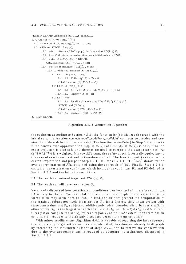
4.4. VERIFICATION OF SAFETY PROPERTIES 49
function GRAPH=Verification (ΣPWA,X (0), U ,Kmax)
1. GRAPH.init({(Xi(0) × U)(0)}n0i=1);
1.1. STACK.push((Xi(0) × U)(0)), i = 1, . . . , n0;
1.2. while not STACK.isEmpty(),
1.2.1. XUf = XU(k) = STACK.pop(), let i such that XU(k) ⊆ Pi;
1.2.2. k ← k∗ � minimum arrival time from initial nodes to XU(k);
1.2.3. if XU(k) ⊆ XUj , XUj ∈ GRAPH,
GRAPH.connect(XUj ,XUf ,0), next();
1.2.4. if relaxedSafe(XU(k),{Zj}nf
j=1), next();
1.2.4.1. while not terminate(XU(k),Kmax),
1.2.4.1.1. for j = 1, . . . , nf ,
1.2.4.1.1.1. if XU(k)⋂
(Zj × U) �= ∅,GRAPH.connect(Zj ,XUf ,k − k∗);
1.2.4.1.2. if (XU(k)) ⊆ Pi,
1.2.4.1.2.1. k ← k + 1;X (k)← [Ai Bi]XU(k − 1) + fi;
1.2.4.1.2.2. XU(k) = X (k)× U ;
1.2.4.1.3. else
1.2.4.1.3.1. for all h �= i such that XUh � Ph⋂ XU(k) �= ∅,
STACK.push( XUh�);GRAPH.connect( XUh�,XUf ,k = k∗);
1.2.4.1.3.2. XU(k)← (X (k) × U)⋂ Pi;
2. return GRAPH.
Algorithm 4.4.1: Verification Algorithm
the evolution according to Section 4.3.1, the function init() initializes the graph with theinitial sets, the function connect(nodeTo,nodeFrom,arcWeight) connects two nodes and cre-ates the node nodeTo if it does not exist. The function relaxedSafe() in Step 1.2.4. checksif the convex over approximation Ck([I 0]XU(k)) of Reachk([I 0]XU(k)) is safe, if so theexact evolution is also safe and there is no need to compute the exact reach set. AsCk([I 0]XU(k)) is a weighted Minkowski’s sum, the safety check is formally equivalent tothe case of exact reach set and is therefore omitted. The function next() exits from thecurrent exploration and jumps to Step 1.2.1.. In Steps 1.2.4.1.3.1., �XUh� stands for theover approximation of XUh obtained using the approach of [19]. Finally, Step 1.2.4.1.contains the termination conditions which include the conditions F1 and F2 defined inSection 4.2.2 and the following conditions:
F3 The reach set entered target set XU(k) ⊆ Zi,
F4 The reach set will never exit region Pi.
We already discussed how containment conditions can be checked, therefore conditionF3 is easy to check. Condition F4 deserves some more explanation, as in the givenformulation may seem hard to test. In [98], the authors present the computation ofthe maximal robust positively invariant set O∞ for a discrete-time linear system withstate constraints x ∈ Pi, subject to additive polyhedral bounded disturbances u ∈ U . Inother words O∞ is the largest set such that [x(k) ∈ O∞] ⇒ [x(k + t) ∈ O∞, ∀u ∈ U , ∀t > 0].Clearly if we compute the set Oi∞ for each region Pi of the PWA system, then terminationcondition F4 reduces to the already discussed set containment condition.
With minor modifications Algorithm 4.4.1 is capable of reporting the first sequencethat enters any target set as soon as it is identified, to refine an already built graphby increasing the maximum number of steps Kmax, and to remove the conservatismdue to the over approximations introduced by adopting the techniques discussed inSection 4.3.1.
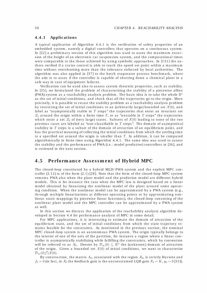
50 CHAPTER 4. REACHABILITY ANALYSIS
4.4.1 Applications
A typical application of Algorithm 4.4.1 is the verification of safety properties of anembedded system, namely a digital controllers that operates on a continuous system.In [32] a preliminary version of this algorithm was used to asses the maximum excur-sion of the height of an electronic car suspension system, and the computational timeswere comparable to the those achieved by using symbolic approaches. In [131] the au-thors verified if a cruise control is able to reach the speed set point within a maximumtime without overshooting more than the tolerance enforced by local authorities. Thealgorithm was also applied in [37] to the batch evaporator process benchmark, wherethe aim is to asses if the controller is capable of shutting down a chemical plant in asafe way in case of equipment failures.
Verification can be used also to assess system theoretic properties, such as stability.In [35], we formulated the problem of characterizing the stability of a piecewise affine(PWA) system as a reachability analysis problem. The basic idea is to take the whole R
n
as the set of initial conditions, and check that all the trajectories go to the origin. Moreprecisely, it is possible to recast the stability problem as a reachability analysis problemby restricting the set of initial conditions to an (arbitrarily large) bounded set X (0), andlabel as “asymptotically stable in T steps” the trajectories that enter an invariant setZ1 around the origin within a finite time T , or as “unstable in T steps” the trajectorieswhich enter a set Z2 of (very large) states. Subsets of X (0) leading to none of the twoprevious cases are labeled as “non-classifiable in T steps”. The domain of asymptoticalstability in T steps is a subset of the domain of attraction of an equilibrium point, andhas the practical meaning of collecting the initial conditions from which the settling timeto a specified set around the origin is smaller than T . In addition, it can be computedalgorithmically in finite time using Algorithm 4.4.1. The same idea was used to assessthe stability and the performance of PWA (i.e.: model predictive) controllers in [36], andis reviewed in the next section.
4.5 Performance Assessment of Hybrid MPC
The closed-loop constituted by a hybrid MLD/PWA system and the explicit MPC con-troller (3.12) is of the form (2.1) [28]. Note that the form of the closed-loop MPC systemremains PWA also when the plant model and the prediction model are different hybridmodels. This is for instance the case when the MPC law is designed based on a linearmodel obtained by linearizing the nonlinear model of the plant around some operat-ing condition. When the nonlinear model can be approximated by a PWA system (e.g.,through multiple linearizations at different operating points or by approximating non-linear static mappings by piecewise linear functions), the closed-loop consisting of thenonlinear plant model and the MPC controller can be approximated by a PWA systemas well.
In this section we discuss the application of the reachability analysis algorithm de-veloped in Section 4.4 for performance analysis of MPC in some detail.
For MPC applications, it is interesting to estimate the domain of attraction of theequilibrium state, and the set of initial conditions from which the state trajectory re-mains feasible for the constraints. As mentioned in the previous section, the nominalMPC closed-loop system is an autonomous PWA system. The origin typically belongs tothe interior of one of the sets of the partition, for instance a region where a linear con-troller is asymptotically stabilizing while fulfilling the constraints, which by conventionwill be referred to as X0. Denote by D∞(0) ⊆ R
n the (unknown) domain of attractionof the origin. Given a bounded set X (0) of initial conditions, we want to characterizeD∞(0)
⋂X (0).
By construction, the matrix A0, associated with the region X0, is strictly Hurwitz andf0 = 0 (in fact, in X0 the feedback gain is the unconstrained LQR gain F0 = K, g0 = 0 [33]).

4.5. PERFORMANCE ASSESSMENT OF HYBRID MPC 51
Then we can compute an invariant set in X0. In particular, we compute the maximumoutput admissible set (MOAS) X∞ ⊆ X0. X∞ is the largest invariant set contained inX0, which by construction of X0 is compatible with the constraints umin ≤ Kx(t) ≤ umax,xmin ≤ x(t) ≤ xmax. By [80, Th.4.1], MOAS is a polyhedron with a finite number of facets,and is computed through a finite number of linear programs (LP’s) [80].
In order to circumvent the undecidability of stability, we give the following
Definition 5 Consider the PWA system (2.1), and let the origin 0 ∈◦X 0 � {x : H0x < S0},
and A0 be strictly Hurwitz. Let X∞ be the maximum output admissible set (MOAS) in X0,which is an invariant for the linear system x(t+ 1) = A0x(t). Let T be a finite time horizon.Then, the set X (0) ⊆ R
n of initial conditions is said to belong to the domain of attractionin T steps DT (0) of the origin if ∀x(0) ∈ X (0) the corresponding final state x(T ) ∈ X∞.
Note that DT (0) ⊆ DT+1(0) ⊆ D∞(0), and DT (0) → D∞(0) as T → ∞. The horizon T isa practical information about the speed of convergence of the PWA system to the originand thus about its dynamic performance.
Definition 6 Consider the PWA system (2.1), and let Xinfeas � Rn\ ∪s
i=1 Xi. The set X (0) ⊆R
n of initial conditions is said to belong to the domain of infeasibility in T steps IT (0) if∀x(0) ∈ X (0) there exists t, 0 ≤ t ≤ T such that x(t) ∈ Xinfeas.
In Definition (6), the set Xinf must be interpreted as a set of “very large” states. Al-though instability in T steps does not guarantee instability (for any finite T , a trajectorymight reach Xinf and converge back to the origin), it has the practical meaning of labelingas “unstable” the trajectories whose magnitude is unacceptable, for instance becausethe PWA system is no longer valid as a model of the real system.
Given a set of initial conditions X (0), we aim at finding subsets of X (0) which aresafely asymptotically stable (X (0)
⋂DT (0)), and subsets which lead to infeasibility in
T steps (X (0)⋂IT (0)). Subsets of X (0) leading to none of the two previous cases are
labeled as non-classifiable in T steps As we will use linear optimization tools, we assumethat X (0) is a convex polyhedral set (or the union of convex polyhedral sets). Typically,non-classifiable subsets shrink and eventually disappear for increasing T .
Example 4.5.1 Consider the system y(t) = s+1s2+s+2u(t), sample the dynamics with T =
0.2 s, and obtain the state-space representation{x(t+ 1) =
[0.7839 −0.17880.3577 0.9627
]x(t) + [ 0.1788
0.0372 ]u(t)
y(t) = [ 1 0.5 ]x(t)(4.6)
The task is to regulate the system to the origin while fulfilling the constraints −1 ≤u(t) ≤ 1 and x(t) ≥
[−0.5−0.5
]. To this aim, we design a linear MPC controller based on the
optimization problem
minut,ut+1
||xt+2|t||2P +1∑
k=0
||xt+k|t||2 + .1||ut+k||2
s.t. −2 ≤ ut+k ≤ 2, k = 0, 1xt+k|t ≥ xmin, xmin �
[−0.5−0.5
], k = 0, 1
(4.7)
where P is the solution to the Riccati equation (in this example Q = [ 1 00 1 ], R = 0.1,
Nu = Ny = Nc = 2). Note that this choice of P corresponds to setting ut+k = Kxt+k|t fork ≥ 2, where K is the LQR gain, and minimizes
∑∞k=0 x
′t+k|txt+k|t + .01u2
t+k with respectto ut, ut+1. The closed loop response from the initial condition x(0) = [1 1]′ is shown inFig. 4.6(a).
The solution to the mp-QP problem was computed by using the solver in [33] in 0.66 son a PC Pentium III 650 MHz running Matlab 5.3, and the corresponding polyhedral
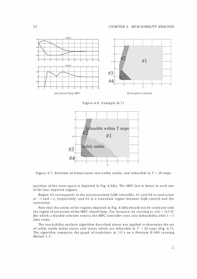
52 CHAPTER 4. REACHABILITY ANALYSIS
(a) Closed-loop MPC
-1 0 1 2 3 4 5
x2
x1
#5
#1#2
#3
#4-1
0
1
2
3
4
5
(b) Explicit solution
Figure 4.6: Example (4.7)
-1 0 1 2 3 4 5
-1
0
1
2
3
4
5
x2
x1
#5#5
Safely stable
Infeasible within T steps
#1#2
#3
#4
Figure 4.7: Partition of initial states into safely stable, and infeasible in T = 20 steps
partition of the state-space is depicted in Fig. 4.6(b). The MPC law is linear in each oneof the four depicted regions.
Region #3 corresponds to the unconstrained LQR controller, #1 and #4 to saturationat −1 and +1, respectively, and #2 is a transition region between LQR control and thesaturation.
Note that the union of the regions depicted in Fig. 4.6(b) should not be confused withthe region of attraction of the MPC closed-loop. For instance, by starting at x(0) = [3.5 0]′
(for which a feasible solution exists), the MPC controller runs into infeasibility after t = 5time steps.
The reachability analysis algorithm described above was applied to determine the setof safely stable initial states and states which are infeasible in T = 20 steps (Fig. 4.7).The algorithm computes the graph of evolutions in 115 s on a Pentium II 400 runningMatlab 5.3.
�
4.6. OPTIMAL CONTROL SOLUTIONS BASED ON REACHABILITY ANALYSIS 53
4.6 Optimal Control Solutions Based on Reachability Anal-ysis
Consider the following optimal control problem
Jopt = minUK−1
0
{‖x(K)−xf‖2
P +K−1∑k=0
‖u(k)‖2R+‖x(k)−xf‖2
Q
}(4.8a)
s.t.
x′(k) = Ai(k)x(k)+Bi(k)u(k)+fi(k) for[
x(k)u(k)
]∈ Pi(k)
umin ≤ u(k) ≤ umax, k = 0, 1, . . . , K−1xmin ≤ x(k) ≤ xmax, k = 1, . . . , Kx(0) = x0
i(k) ∈ {1, . . . , s}x(K) ∈ Zfin
(4.8b)
where K is the prediction horizon, P , Q and R are positive definite weighting matrices,x(k) is the state evolved at time k by applying the input sequence Uk−1
0 � {u(0), . . . , u(k−1)}to (2.1) from the initial state x(0) = x0, i(k) ∈ {1, . . . , s} is the index such that Equa-tions (2.1c)-(2.1c) are satisfied, xf and Zfin are a reference state and a polyhedral finaltarget set, respectively 7, umin, umax and xmin, xmax are hard bounds on inputs and states,respectively. The sets U � {u : umin ≤ u ≤ umax} and Zsafe � {x : xmin ≤ x ≤ xmax} will beused in the sequel for compactness of notation8. In this section we exploit the ideas ofthe reachability analysis algorithm proposed in Section 4.2 in order to solve the optimalcontrol problem (4.8).
Remark 4.6.1 For ease of notation, we have supposed that the weighting matrices areconstant with respect to i (=space) and k (=time). Nonetheless, the proposed frameworkcan easily handle the case of region-dependent and/or time-varying weights Ri(k)(k),Qi(k)(k). This feature is helpful for instance when the index i reflects different plantoperation modes. The same extension can be done for the input and state limits umin,umax, xmin, xmax.
�
Remark 4.6.2 Existing heuristic information about the expected optimal schedule canbe easily embedded into (4.8). In fact, when heuristics are given as space/time “land-marks” to be hit, such requirements can be expressed in (4.8) as additional constraintsof the form x(k) ∈ Zheur[kmin, kmax], where Zheur[kmin, kmax] represents the landmark areain the state-space to be reached at time k ∈ [kmin, kmax].
�By taking into account the equivalence between PWA and MLD systems (2.20) men-
tioned in Chapter 2, the optimization problem (4.8) can be reformulated as the mixed-integer quadratic programming (MIQP) problem
Jopt = minUK−1
0
{‖x(K)−xf‖2
P +
K−1∑k=0
‖u(k)‖2R+‖x(k)−xf‖2
Q
}(4.9a)
s.t.
x′(k) = Ax(k) + B1u(k) + B2δ(k) + B3z(k)E2δ(k) + E3z(k) ≤ E1u(k) + E4x(k) + E5
umin ≤ u(k) ≤ umax, k = 0, 1, . . . , K−1xmin ≤ x(k) ≤ xmax, k = 1, . . . , Kx(0) = x0
δ(k) ∈ {0, 1}rb
x(K) ∈ Zfin
(4.9b)
7For instance, Zfin can be a satisfactory range around the equilibrium xf8More in general, the sets U and Zsafe could also be polyhedral
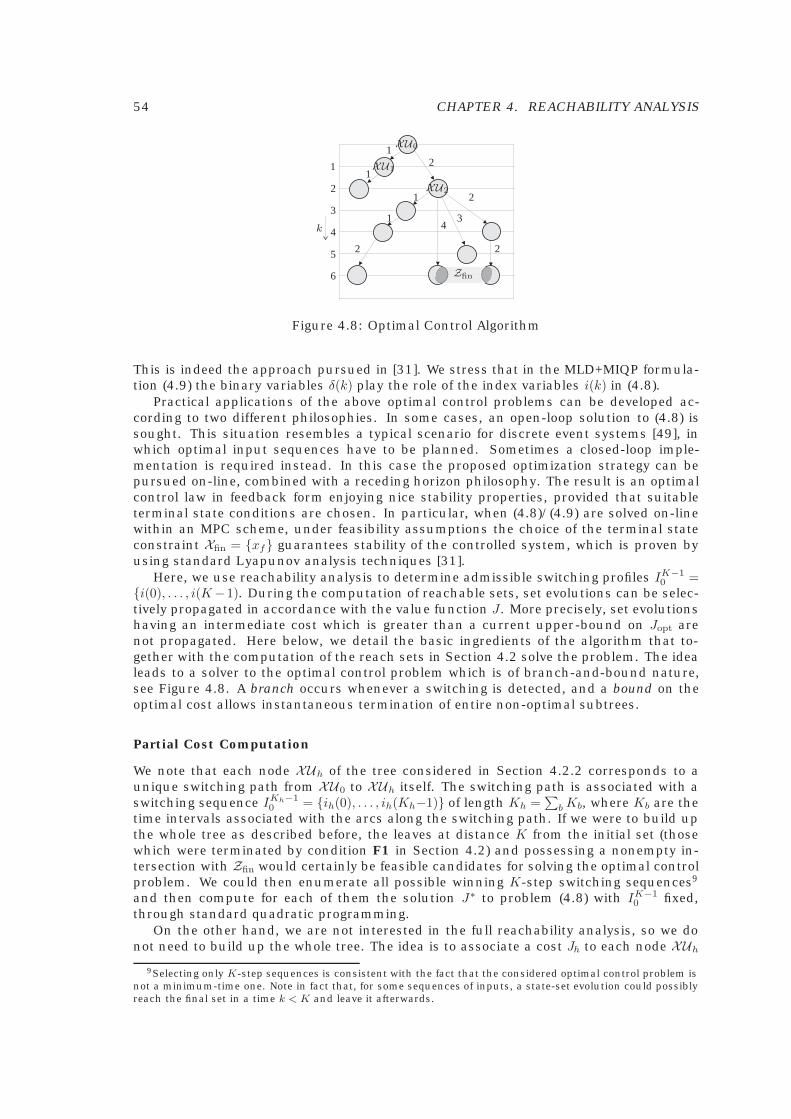
54 CHAPTER 4. REACHABILITY ANALYSIS
XU0
XU1
XU2
Zfin
1
1
11
1
2 2
22
2
33
44
5
6
k
Figure 4.8: Optimal Control Algorithm
This is indeed the approach pursued in [31]. We stress that in the MLD+MIQP formula-tion (4.9) the binary variables δ(k) play the role of the index variables i(k) in (4.8).
Practical applications of the above optimal control problems can be developed ac-cording to two different philosophies. In some cases, an open-loop solution to (4.8) issought. This situation resembles a typical scenario for discrete event systems [49], inwhich optimal input sequences have to be planned. Sometimes a closed-loop imple-mentation is required instead. In this case the proposed optimization strategy can bepursued on-line, combined with a receding horizon philosophy. The result is an optimalcontrol law in feedback form enjoying nice stability properties, provided that suitableterminal state conditions are chosen. In particular, when (4.8)/(4.9) are solved on-linewithin an MPC scheme, under feasibility assumptions the choice of the terminal stateconstraint Xfin = {xf} guarantees stability of the controlled system, which is proven byusing standard Lyapunov analysis techniques [31].
Here, we use reachability analysis to determine admissible switching profiles IK−10 =
{i(0), . . . , i(K−1). During the computation of reachable sets, set evolutions can be selec-tively propagated in accordance with the value function J. More precisely, set evolutionshaving an intermediate cost which is greater than a current upper-bound on Jopt arenot propagated. Here below, we detail the basic ingredients of the algorithm that to-gether with the computation of the reach sets in Section 4.2 solve the problem. The idealeads to a solver to the optimal control problem which is of branch-and-bound nature,see Figure 4.8. A branch occurs whenever a switching is detected, and a bound on theoptimal cost allows instantaneous termination of entire non-optimal subtrees.
Partial Cost Computation
We note that each node XUh of the tree considered in Section 4.2.2 corresponds to aunique switching path from XU0 to XUh itself. The switching path is associated with aswitching sequence IKh−1
0 = {ih(0), . . . , ih(Kh−1)} of length Kh =∑
b Kb, where Kb are thetime intervals associated with the arcs along the switching path. If we were to build upthe whole tree as described before, the leaves at distance K from the initial set (thosewhich were terminated by condition F1 in Section 4.2) and possessing a nonempty in-tersection with Zfin would certainly be feasible candidates for solving the optimal controlproblem. We could then enumerate all possible winning K-step switching sequences9
and then compute for each of them the solution J∗ to problem (4.8) with IK−10 fixed,
through standard quadratic programming.On the other hand, we are not interested in the full reachability analysis, so we do
not need to build up the whole tree. The idea is to associate a cost Jh to each node XUh
9Selecting only K-step sequences is consistent with the fact that the considered optimal control problem isnot a minimum-time one. Note in fact that, for some sequences of inputs, a state-set evolution could possiblyreach the final set in a time k < K and leave it afterwards.
4.6. OPTIMAL CONTROL SOLUTIONS BASED ON REACHABILITY ANALYSIS 55
by computing the intermediate minimum cost from XU0 to the corresponding region,given by the solution of the following quadratic program
Jh = minU
Kh−10
J(UKh−10 , 0,Kh) (4.10a)
s.t.
x′(k) = Aih(k)x(k)+Bih(k)u(k)+fih(k) for[
x(k)u(k)
]∈ Pih(k)
umin ≤ u(k) ≤ umax, k = 0, 1, . . . ,Kh−1xmin ≤ x(k) ≤ xmax, k = 1, . . . ,Kh
x(Kh) ∈ XUh
x(0) = x0
(4.10b)
where IKh−10 = {ih(0), . . . , ih(Kh−1)} is the corresponding switching sequence, and
J(UKf−1Ki
,Ki,Kf) �
Kf−1∑
k=Ki
‖u(k)‖2R + ‖x(k)− xf‖2Q
.
When no feasible solution to (4.10) exists, we conventionally set Jh = +∞. The advantageprovided by these additional calculations is that — once the target region is eventuallyreached in K steps and we can compute an upper bound J∗ on the overall cost —we have an additional termination condition. More precisely, as soon as an evolutionintersects Zfin at k = K, we compute J∗ as described before and enforce the followingnew termination condition
F5 Jh ≥ J∗, the intermediate cost exceeds or is equal to the current upper bound10.
Whenever a new exploration reaches Zfin in K steps with a lower cost, the upperbound J∗ is updated, along with the the correspoding minimizer U∗ = arg minJ∗. Notethat we can still use the hyper-rectangular approximation and that the partial costcomputation is also able to rule out possible infeasible switches as soon as they aredetected. In fact, in this case at least one of the intermediate optimal control problemsassociated to the child nodes will be infeasible.
Node Selection Criterion
The last point to be addressed is the choice of an effective exploration strategy, that is,the ordering criterion according to which new nodes are taken from the list and explored.In order to reduce fruitless explorations, an adequate strategy should recognize the morepromising paths to be searched. To this purpose, we suggest the following node selectioncriterion
NS1 Select the node having the smallest associated normalized cost Jh � Jh/Kh
where, for convenience, we set J0 = J0 = 0. The normalization factor 1/Kh is instrumen-tal to the proposed performance-driving mechanism. In fact, it penalizes, among se-quences characterized by identical intermediate cost Jh, those sequences with a smallerminimum cumulated time Kh, which therefore have a larger time-to-go, and are morelikely to give rise to a higher overall cost J∗. As a result, the exploration is guided byperformance in the sense that the procedure aims at reaching the target set Zfin throughthe most promising evolutions. This strategy leads to tighter upper bounds J∗, and thusto a more effective termination condition F5.
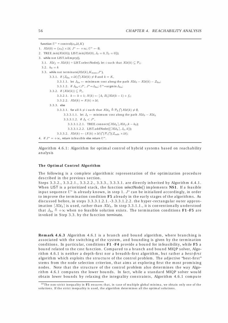
56 CHAPTER 4. REACHABILITY ANALYSIS
function U∗ = control(x0,U ,K)
1. XU(0) = {x0} × U ; J∗ ← +∞; U∗ ← ∅;2. TREE.init(XU(0)); LIST.init(XU(0), J0 = 0, T0 = 0});3. while not LIST.isEmpty(),
3.1. XUf = XU(k) = LIST.selectNode(), let i such that XU(k) ⊆ Pi;
3.2. k0 = k
3.3. while not terminate(XU(k),Kmax,J∗),
3.3.1. if (Zfin × U)⋂ XU(k) �= ∅ and k = K,
3.3.1.1. let Jfin ← minimum cost along the path XU0 − XU(k)− Zfin;
3.3.1.2. if Jfin<J∗, J∗=Jfin; U∗=argminJfin;
3.3.2. if (XU(k)) ⊆ Pi,
3.3.2.1. k ← k + 1; X (k)← [Ai Bi]XU(k − 1) + fi;
3.3.2.2. XU(k) = X (k)× U ;
3.3.3. else
3.3.3.1. for all h �= i such that XUh � Ph⋂XU(k) �= ∅,
3.3.3.1.1. let Jh ← minimum cost along the path XU0 −XUh
3.3.3.1.2. if Jh < J∗,
3.3.3.1.2.1. TREE.connect( XUh�,XUf ,k − k0);
3.3.3.1.2.2. LIST.addNode({ XUh�, Jh, k});3.3.3.2. XU(k)← (X (k)× U)
⋂Pi⋂
(Zsafe × U);
4. if J∗ = +∞, return infeasible else return U∗.
Algorithm 4.6.1: Algorithm for optimal control of hybrid systems based on reachabilityanalysis
The Optimal Control Algorithm
The following is a complete algorithmic representation of the optimization proceduredescribed in the previous section.Steps 3.3.2., 3.3.2.1., 3.3.2.2., 3.3.3., 3.3.3.1. are directly inherited by Algorithm 4.4.1.When LIST is a prioritized stack, the function selectNode() implements NS1. If a feasibleinput sequence U∗ is already known, in step 1. J∗ can be initialized accordingly, in orderto improve the termination condition F5 already in the early stages of the algorithms. Asdiscussed before, in steps 3.3.3.1.2.1. -3.3.3.1.2.2. the hyper-rectangular outer approx-imation �XUh� is used, rather than XUh. In step 3.3.1.1., it is conventionally understoodthat Jfin � +∞ when no feasible solution exists. The termination conditions F1–F5 areinvoked in Step 3.3. by the function terminate.
Remark 4.6.3 Algorithm 4.6.1 is a branch and bound algorithm, where branching isassociated with the switching of the system, and bounding is given by the terminationconditions. In particular, conditions F1 -F4 provide a bound for infeasibility, while F5 abound related to the cost function. Compared to a branch and bound MIQP solver, Algo-rithm 4.6.1 is neither a depth-first nor a breadth-first algorithm, but rather a best-firstalgorithm which exploits the structure of the control problem. The adjective “best-first”stems from the node selection criterion, that aims at exploring first the most promisingnodes. Note that the structure of the control problem also determines the way Algo-rithm 4.6.1 computes the lower bounds. In fact, while a standard MIQP solver wouldobtain lower bounds by relaxing the integrality constraints, Algorithm 4.6.1 compute
10The non-strict inequality in F5 ensures that, in case of multiple global minima, we obtain only one of thesolutions. If the strict inequality is used, the algorithm determines all the optimal solutions.
4.6. OPTIMAL CONTROL SOLUTIONS BASED ON REACHABILITY ANALYSIS 57
lower bounds by optimizing over reachable sub-paths. Even though the worst-case per-formance of this algorithm is lower with respect to plain enumeration, as in generalare branch and bound algorithms, the proposed method is considerably faster in theaverage.
�Clearly the node selection criterion NS1 could be augmented to take into account
landmarks and select first the evolutions that match a spatial and temporal landmarkZheur[kmin, kmax].
Remark 4.6.4 When binary inputs uj(k) ∈ {0, 1} are present (mb �= 0), they can be han-dled as shown in [117]. In the particular case where the dynamics of the system issimply linear (s = 1), the algorithm executes just one single QP (as only one reach-setcomputation is performed), in accordance with non-hybrid, conventional finite-horizonlinear quadratic solvers.
�
4.6.1 Variations to the Optimization Algorithm
One of the key steps of the optimization algorithm described in the previous section isthe computation of the intermediate costs Jh. The approach proposed in Algorithm 4.6.1solves problem (4.10) at each switching detection. This is computationally expensive,since the number of free inputs (and therefore the computation time for solving the QP)grows as the exploration proceeds.
In this section we propose some alternatives to the termination condition F5 and thenode selection criterion, which can be implemented by computing a lower bound to theintermediate cost Jh, and a lower bound to the cost to go.
Lower Bound to the Intermediate Cost
At each switching detection the minimum cost to get from the father node XU f to thenew node XUh can be computed by solving a QP. Let Kf be the length of the switchingsequence associated with the father node XUf , and let if be the region index associatedwith the father node, the node-to-node cost Jb from Gf to Gk is defined as
Jb = minU
Kh−1Kf
J(UKh−1Kf
,Kf ,Kh) (4.11a)
s.t.
x′(k) = Aifx(k) +Bif
u(k) + fif, for
[x(k)u(k)
]∈ Pif
umin ≤ u(k) ≤ umax, k = Kf , . . . ,Kh−1xmin ≤ x(k) ≤ xmax, t = Kf + 1, . . . ,Kh
x(Kf ) ∈ XUf
x(Kh) ∈ XUh .
(4.11b)
Node-to-node costs are clearly properties of the arcs of the tree, exactly as transitiontimes, and the time required for their computation depends on the inter-switching time,Kh−Kf , but, contrarily to the partial costs Jh computed in (4.10), does not grow with theabsolute time Kh, Kf . The sum of all node-to-node costs along the path to region XUh
is a lower bound to Jh. The reason for this is simply explained in Fig. 4.9). Compared tothe partial cost Jh associated with the path XU0 − XUf − XUh, the sum of the node-to-node costs Jf + Jb is computed with one extra artificial degree of freedom, namely thatx1 and x2 can be different.
Note that using a lower bound to Jh, although cheaper to compute, is less effectivewhen used in place of the exact value in the termination condition F5, and renders thenode selection criterion less accurate.
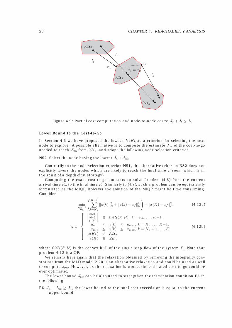
58 CHAPTER 4. REACHABILITY ANALYSIS
XU0
XUf
XUh
x1x1 = x2
x2
Jh
Jb
Jf
Figure 4.9: Partial cost computation and node-to-node costs: Jf + Jb ≤ Jh
Lower Bound to the Cost-to-Go
In Section 4.6 we have proposed the lowest Jh/Kh as a criterion for selecting the nextnode to explore. A possible alternative is to compute the estimate Jres of the cost-to-goneeded to reach Zfin from XUh, and adopt the following node selection criterion
NS2 Select the node having the lowest Jh + Jres
Contrarily to the node selection criterion NS1, the alternative criterion NS2 does notexplicitly favors the nodes which are likely to reach the final time T soon (which is inthe spirit of a depth-first strategy).
Computing the exact cost-to-go amounts to solve Problem (4.8) from the currentarrival time Kh to the final time K. Similarly to (4.9), such a problem can be equivalentlyformulated as the MIQP, however the solution of the MIQP might be time consuming.Consider
minUK−1
Kh
(K−1∑k=Kh
‖u(k)‖2R + ‖x(k)− xf‖2Q
)+ ‖x(K)− xf‖2P (4.12a)
s.t.
[x(k)u(k)
x′(k)
]∈ CXU(X ,U), k = Kh, . . . ,K−1,
umin ≤ u(k) ≤ umax, k = Kh, . . . ,K−1,xmin ≤ x(k) ≤ xmax, k = Kh + 1, . . . ,K,
x(Kh) ∈ XUh,x(K) ∈ Zfin,
(4.12b)
where CXU(X ,U) is the convex hull of the single step flow of the system Σ. Note thatproblem 4.12 is a QP.
We remark here again that the relaxation obtained by removing the integrality con-straints from the MLD model 2.20 is an alternative relaxation and could be used as wellto compute Jres. However, as the relaxation is worse, the estimated cost-to-go could beover optimistic.
The lower bound Jres can be also used to strengthen the termination condition F5 inthe following
F6 Jh + Jres ≥ J∗, the lower bound to the total cost exceeds or is equal to the currentupper bound
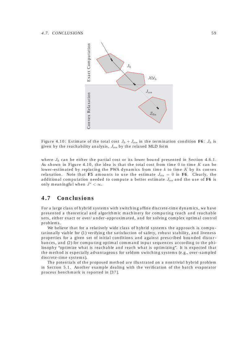
4.7. CONCLUSIONS 59
Con
vex
Rel
axa
tion
Exa
ctC
omp
uta
tion
XUh
Jh
Jres
Zfin
Figure 4.10: Estimate of the total cost Jh + Jres in the termination condition F6: Jh isgiven by the reachability analysis, Jres by the relaxed MLD form
where Jh can be either the partial cost or its lower bound presented in Section 4.6.1.As shown in Figure 4.10, the idea is that the total cost from time 0 to time K can belower-estimated by replacing the PWA dynamics from time k to time K by its convexrelaxation. Note that F5 amounts to use the estimate Jres = 0 in F6. Clearly, theadditional computation needed to compute a better estimate Jres and the use of F6 isonly meaningful when J∗ <∞.
4.7 Conclusions
For a large class of hybrid systems with switching affine discrete-time dynamics, we havepresented a theoretical and algorithmic machinery for computing reach and reachablesets, either exact or over/under-approximated, and for solving complex optimal controlproblems.
We believe that for a relatively wide class of hybrid systems the approach is compu-tationally viable for (1) verifying the satisfaction of safety, robust stability, and livenessproperties for a given set of initial conditions and against prescribed bounded distur-bances, and (2) for computing optimal command input sequences according to the phi-losophy “optimize what is reachable and reach what is optimizing”. It is expected thatthe method is especially advantageous for seldom switching systems (e.g., over-sampleddiscrete-time systems).
The potentials of the proposed method are illustrated on a nontrivial hybrid problemin Section 5.1. Another example dealing with the verification of the batch evaporatorprocess benchmark is reported in [37].

60 CHAPTER 4. REACHABILITY ANALYSIS
Chapter 5
Application Examples
5.1 Analysis and Control of a Cruise Control System
In this section we use HYSDEL to obtain a hybrid model of a car with robotized manualgear shift, and show how such a model can be directly used (i) to formally verify certainsafety and liveness properties of a simple cruise controller based on PI control and a setof gear-switching rules and (ii) to synthesize a cruise control system that is piecewiseaffine and optimal with respect to a certain performance index.
5.1.1 Car model
We focus on a car equipped with manual transmission, and we assume that the gearcommand is robotized, namely that a slave control system takes care of releasing theclutch, shifting the gear, and engaging the clutch. We only consider the longitudinaldynamics of the car: the continuous variables are the scalar position x (m) and thespeed v = x (m·s−1). The continuous inputs are the engine torque ut (Nm), the brakingforce ub (N), and the sinus of the road slope us, plus six binary inputs g1, g2, g3, g4, g5 andgR ∈ {0, 1} corresponding to the selected gear. Denoting by ω the engine speed (rad·s−1),we have the kinematic relation
v =klossrwheel
Rg(i)Rfinω, (5.1)
where Rg(i) is the gear ratio corresponding to the i-th gear, Rfin is the final drive ratio,rwheel is the wheel radius, and kloss is the drive train efficiency level [42]. Note that byusing a kinematic relation for the speed engine, we are neglecting the clutch, the motordynamic behavior, and we are assuming that the time spent for gear shift is negligible.
The dynamic equation of motion of the car is mx = Fe − Fb − Fr − Fs where m (kg) isthe vehicle mass, Fe (N) is the traction force, Fb = ub is the braking force (N), Fr (N) is thefriction force, and Fs (N) takes into account the slope of the road. Fs = mgus (N), whereus = sinα and α is the slope of the road and as a first approximation, we assume thatFr is linear in v, Fr = βv, where β (kg·m·s−1) is a constant that takes into account allthe frictions (i.e. aerodynamic, tires deformation, drive train). From the conservation ofmechanical power, we have Fev = ωu1, which gives Fe = kloss
Rg(i)u1. The commanded torqueut is upper-bounded by the maximum torque deliverable at a certain engine speed ω,ut ≤ C+
e (ω) where C+e (ω) is a nonlinear function typically reported in the data sheets of
the car and C−e (ω) is the maximum braking force that the engine can provide when the
throttle is fully released. In order to derive a hybrid model of the car as described inSection 2.2, we piecewise-linearize C+
e (ω) into four regions using the PWL toolbox [96],which requires the introduction of three event variables δPWL1, δPWL2, δPWL3, and as afirst approximation, we assume C−
e (ω) = −α1 − β1ω, cf. Fig. 5.1.
61
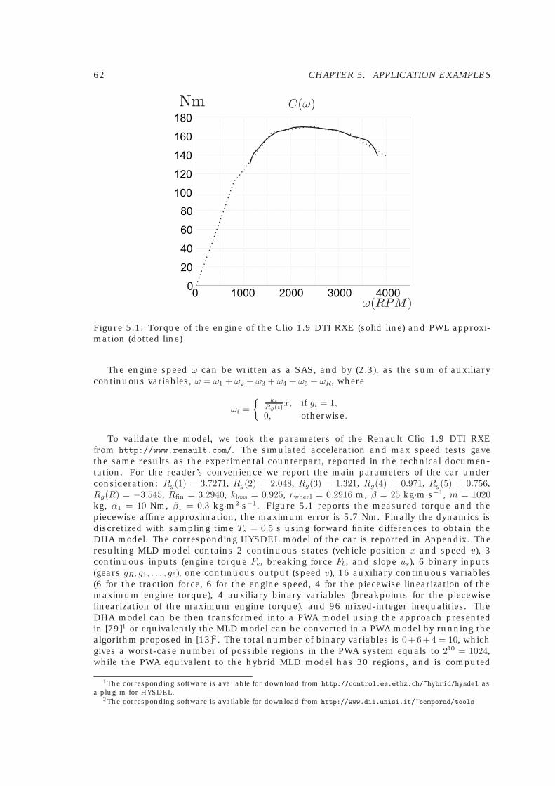
62 CHAPTER 5. APPLICATION EXAMPLES
0 1000 2000 3000 40000
20
40
60
80
100
120
140
160
180
Nm C(!)
!(RPM)
Figure 5.1: Torque of the engine of the Clio 1.9 DTI RXE (solid line) and PWL approxi-mation (dotted line)
The engine speed ω can be written as a SAS, and by (2.3), as the sum of auxiliarycontinuous variables, ω = ω1 + ω2 + ω3 + ω4 + ω5 + ωR, where
ωi ={ ks
Rg(i) x, if gi = 1,0, otherwise.
To validate the model, we took the parameters of the Renault Clio 1.9 DTI RXEfrom http://www.renault.com/. The simulated acceleration and max speed tests gavethe same results as the experimental counterpart, reported in the technical documen-tation. For the reader’s convenience we report the main parameters of the car underconsideration: Rg(1) = 3.7271, Rg(2) = 2.048, Rg(3) = 1.321, Rg(4) = 0.971, Rg(5) = 0.756,Rg(R) = −3.545, Rfin = 3.2940, kloss = 0.925, rwheel = 0.2916 m, β = 25 kg·m·s−1, m = 1020kg, α1 = 10 Nm, β1 = 0.3 kg·m2·s−1. Figure 5.1 reports the measured torque and thepiecewise affine approximation, the maximum error is 5.7 Nm. Finally the dynamics isdiscretized with sampling time Ts = 0.5 s using forward finite differences to obtain theDHA model. The corresponding HYSDEL model of the car is reported in Appendix. Theresulting MLD model contains 2 continuous states (vehicle position x and speed v), 3continuous inputs (engine torque Fe, breaking force Fb, and slope us), 6 binary inputs(gears gR, g1, . . . , g5), one continuous output (speed v), 16 auxiliary continuous variables(6 for the traction force, 6 for the engine speed, 4 for the piecewise linearization of themaximum engine torque), 4 auxiliary binary variables (breakpoints for the piecewiselinearization of the maximum engine torque), and 96 mixed-integer inequalities. TheDHA model can be then transformed into a PWA model using the approach presentedin [79]1 or equivalently the MLD model can be converted in a PWA model by running thealgorithm proposed in [13]2. The total number of binary variables is 0+6+4 = 10, whichgives a worst-case number of possible regions in the PWA system equals to 210 = 1024,while the PWA equivalent to the hybrid MLD model has 30 regions, and is computed
1The corresponding software is available for download from http://control.ee.ethz.ch/~hybrid/hysdel asa plug-in for HYSDEL.
2The corresponding software is available for download from http://www.dii.unisi.it/~bemporad/tools
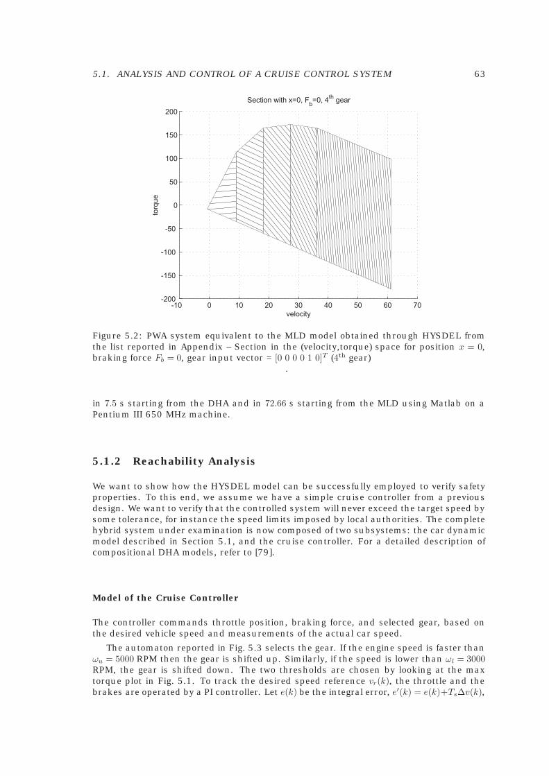
5.1. ANALYSIS AND CONTROL OF A CRUISE CONTROL SYSTEM 63
Figure 5.2: PWA system equivalent to the MLD model obtained through HYSDEL fromthe list reported in Appendix – Section in the (velocity,torque) space for position x = 0,braking force Fb = 0, gear input vector = [0 0 0 0 1 0]T (4th gear)
.
in 7.5 s starting from the DHA and in 72.66 s starting from the MLD using Matlab on aPentium III 650 MHz machine.
5.1.2 Reachability Analysis
We want to show how the HYSDEL model can be successfully employed to verify safetyproperties. To this end, we assume we have a simple cruise controller from a previousdesign. We want to verify that the controlled system will never exceed the target speed bysome tolerance, for instance the speed limits imposed by local authorities. The completehybrid system under examination is now composed of two subsystems: the car dynamicmodel described in Section 5.1, and the cruise controller. For a detailed description ofcompositional DHA models, refer to [79].
Model of the Cruise Controller
The controller commands throttle position, braking force, and selected gear, based onthe desired vehicle speed and measurements of the actual car speed.
The automaton reported in Fig. 5.3 selects the gear. If the engine speed is faster thanωu = 5000 RPM then the gear is shifted up. Similarly, if the speed is lower than ωl = 3000RPM, the gear is shifted down. The two thresholds are chosen by looking at the maxtorque plot in Fig. 5.1. To track the desired speed reference vr(k), the throttle and thebrakes are operated by a PI controller. Let e(k) be the integral error, e′(k) = e(k)+Ts∆v(k),
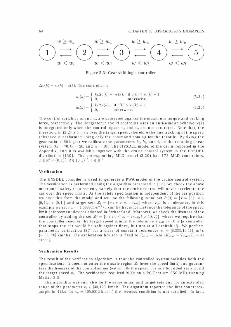
64 CHAPTER 5. APPLICATION EXAMPLES
Figure 5.3: Gear shift logic controller
∆v(k) = vr(k)− v(k). The controller is
ut(k) ={kt∆v(k) + ite(k), if v(k) ≤ vr(k) + 1.0, otherwise,
(5.2a)
ub(k) ={kb∆v(k), if v(k) > vr(k) + 1,0, otherwise.
(5.2b)
The control variables ut and ub are saturated against the maximum torque and brakingforce, respectively. The integrator in the PI controller uses an anti-windup scheme: e(k)is integrated only when the control inputs ut and ub are not saturated. Note that, thethreshold in (5.2) is 1 m/s over the target speed, therefore the fine tracking of the speedreference is performed using only the command coming for the throttle. By fixing thegear ratio in fifth gear we calibrate the parameters kt, kb, and it on the resulting linearsystem (kt = 70, kb = 20, and it = 10). The HYSDEL model of the car is reported in theAppendix, and it is available together with the cruise control system in the HYSDELdistribution [130]. The corresponding MLD model (2.20) has 173 MLD constraints,x ∈ R
2 × {0, 1}5, d ∈ {0, 1}15, z ∈ R19.
Verification
The HYSDEL compiler is used to generate a PWA model of the cruise control system.The verification is performed using the algorithm presented in [37]. We check the abovementioned safety requirement, namely that the cruise control will never accelerate thecar over the speed limits. As the safety specification is independent of the car positionwe omit this from the model and we use the following initial set X (0) = {x = [ v
e ] : v ∈[0, 1], e ∈ [0, 1]} and target set: Z1 = {v : v > vr + rtoll} where rtoll is a tolerance, in thisexample we set rtoll = 1.3889 m·s−1 (5 km/h) that is for instance the tolerance of the speedlimit enforcement devices adopted in Switzerland. Moreover, we check the liveness of thecontroller by adding the set Z2 = {v, t : v ≤ vr − 2rtoll, t > 10/Ts}, where we require thatthe controller reaches the target speed minus the tolerance 2rtoll in 10 s (a controllerthat stops the car would be safe against fines, but not at all desirable!). We performparametric verification [37] for a class of constant references vr ∈ [8.333, 19.444] m/s(= [30, 70] km/h). The exploration horizon is fixed to Tmax = 15.5s (Kmax = Tmax/Ts = 31steps).
Verification Results
The result of the verification algorithm is that the controlled system satisfies both thespecifications: It does not enter the unsafe region Z1 (over the speed limit) and guaran-tees the liveness of the control action (within 10s the speed v is in a bounded set aroundthe target speed vr. The verification required 9109s on a PC Pentium 650 MHz runningMatlab 5.3.
The algorithm was run also for the same initial and target sets and for an extendedrange of the parameter vr ∈ [30, 120] km/h. The algorithm reported the first counterex-ample in 415s: for vr = 105.0012 km/h) the liveness condition is not satisfied. In fact,
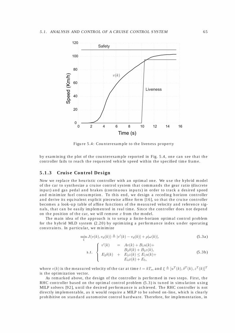
5.1. ANALYSIS AND CONTROL OF A CRUISE CONTROL SYSTEM 65
0 2 4 6 8 10 12 14 160
20
40
60
80
100
120
Time (s)
Speed(Km/h)
Liveness
Safety
v(k)
Figure 5.4: Counterexample to the liveness property
by examining the plot of the counterexample reported in Fig. 5.4, one can see that thecontroller fails to reach the requested vehicle speed within the specified time frame.
5.1.3 Cruise Control Design
Now we replace the heuristic controller with an optimal one. We use the hybrid modelof the car to synthesize a cruise control system that commands the gear ratio (discreteinput) and gas pedal and brakes (continuous inputs) in order to track a desired speedand minimize fuel consumption. To this end, we design a receding horizon controllerand derive its equivalent explicit piecewise affine form [16], so that the cruise controllerbecomes a look-up table of affine functions of the measured velocity and reference sig-nals, that can be easily implemented in real time. Since the controller does not dependon the position of the car, we will remove x from the model.
The main idea of the approach is to setup a finite-horizon optimal control problemfor the hybrid MLD system (2.20) by optimizing a performance index under operatingconstraints. In particular, we minimize
minξJ(v(k), vd(k)) � |v′(k)− vd(k)|+ ρ|ω(k)|, (5.3a)
s.t.
v′(k) = Av(k) +B1u(k)+B2δ(k) +B3z(k),
E2δ(k) + E3z(k) ≤ E1u(k)+E4x(k) + E5,
(5.3b)
where v(k) is the measured velocity of the car at time t = kTs, and ξ � [uT (k), δT (k), zT (k)]T
is the optimization vector.As remarked above, the design of the controller is performed in two steps. First, the
RHC controller based on the optimal control problem (5.3) is tuned in simulation usingMILP solvers [92], until the desired performance is achieved. The RHC controller is notdirectly implementable, as it would require a MILP to be solved on-line, which is clearlyprohibitive on standard automotive control hardware. Therefore, for implementation, in
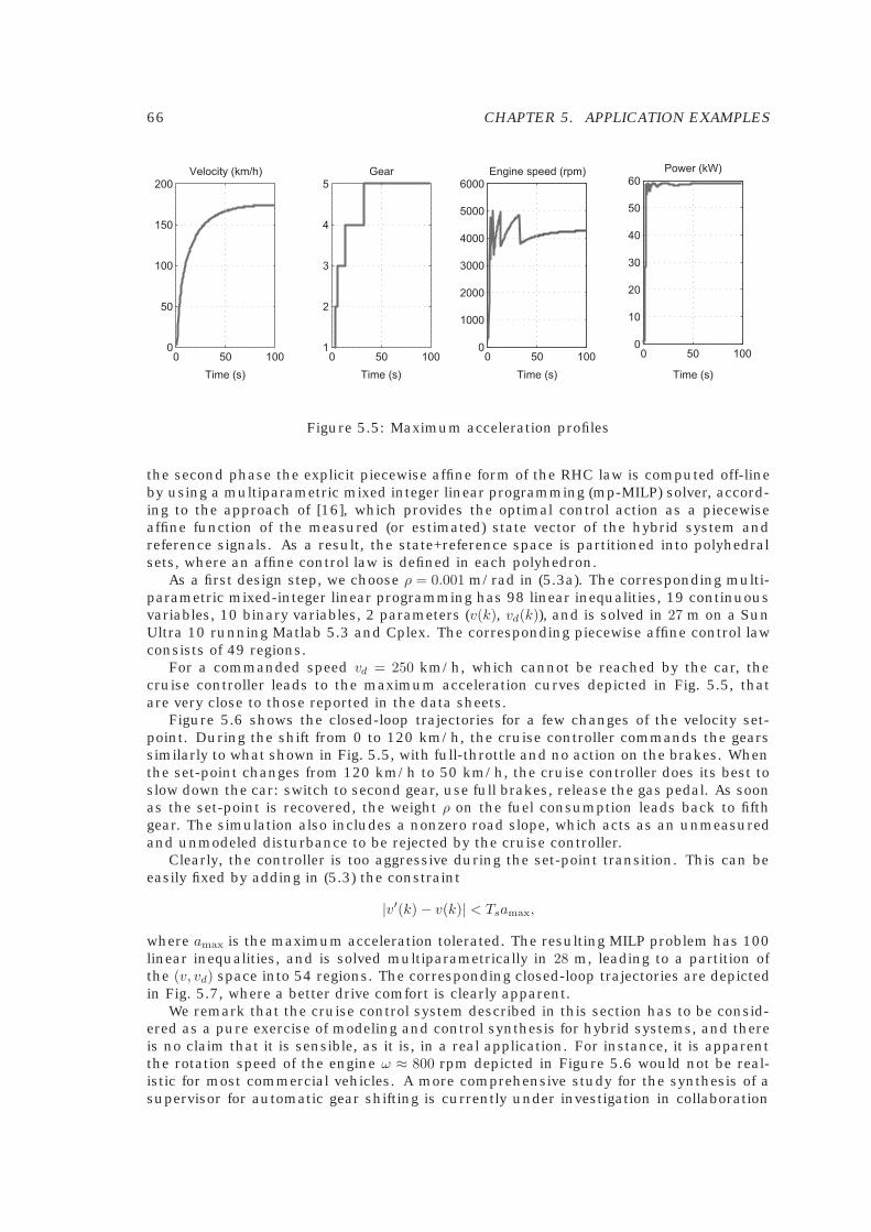
66 CHAPTER 5. APPLICATION EXAMPLES
Figure 5.5: Maximum acceleration profiles
the second phase the explicit piecewise affine form of the RHC law is computed off-lineby using a multiparametric mixed integer linear programming (mp-MILP) solver, accord-ing to the approach of [16], which provides the optimal control action as a piecewiseaffine function of the measured (or estimated) state vector of the hybrid system andreference signals. As a result, the state+reference space is partitioned into polyhedralsets, where an affine control law is defined in each polyhedron.
As a first design step, we choose ρ = 0.001 m/rad in (5.3a). The corresponding multi-parametric mixed-integer linear programming has 98 linear inequalities, 19 continuousvariables, 10 binary variables, 2 parameters (v(k), vd(k)), and is solved in 27 m on a SunUltra 10 running Matlab 5.3 and Cplex. The corresponding piecewise affine control lawconsists of 49 regions.
For a commanded speed vd = 250 km/h, which cannot be reached by the car, thecruise controller leads to the maximum acceleration curves depicted in Fig. 5.5, thatare very close to those reported in the data sheets.
Figure 5.6 shows the closed-loop trajectories for a few changes of the velocity set-point. During the shift from 0 to 120 km/h, the cruise controller commands the gearssimilarly to what shown in Fig. 5.5, with full-throttle and no action on the brakes. Whenthe set-point changes from 120 km/h to 50 km/h, the cruise controller does its best toslow down the car: switch to second gear, use full brakes, release the gas pedal. As soonas the set-point is recovered, the weight ρ on the fuel consumption leads back to fifthgear. The simulation also includes a nonzero road slope, which acts as an unmeasuredand unmodeled disturbance to be rejected by the cruise controller.
Clearly, the controller is too aggressive during the set-point transition. This can beeasily fixed by adding in (5.3) the constraint
|v′(k)− v(k)| < Tsamax,
where amax is the maximum acceleration tolerated. The resulting MILP problem has 100linear inequalities, and is solved multiparametrically in 28 m, leading to a partition ofthe (v, vd) space into 54 regions. The corresponding closed-loop trajectories are depictedin Fig. 5.7, where a better drive comfort is clearly apparent.
We remark that the cruise control system described in this section has to be consid-ered as a pure exercise of modeling and control synthesis for hybrid systems, and thereis no claim that it is sensible, as it is, in a real application. For instance, it is apparentthe rotation speed of the engine ω ≈ 800 rpm depicted in Figure 5.6 would not be real-istic for most commercial vehicles. A more comprehensive study for the synthesis of asupervisor for automatic gear shifting is currently under investigation in collaboration
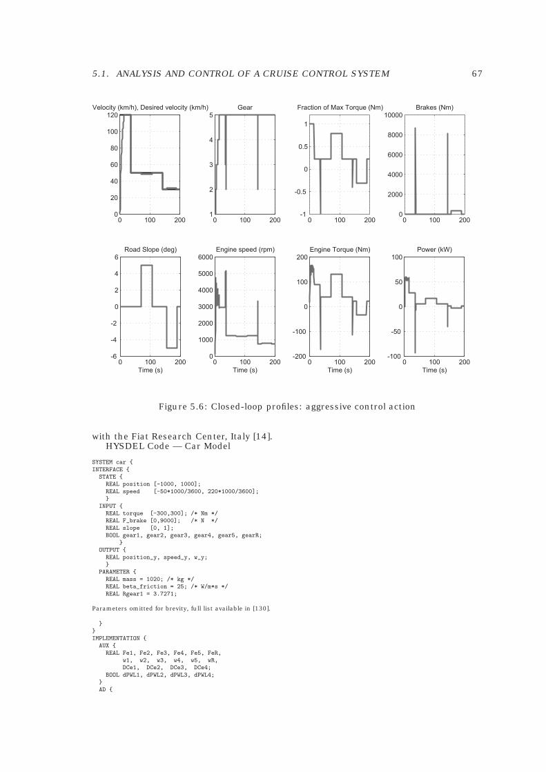
5.1. ANALYSIS AND CONTROL OF A CRUISE CONTROL SYSTEM 67
Figure 5.6: Closed-loop profiles: aggressive control action
with the Fiat Research Center, Italy [14].HYSDEL Code — Car Model
SYSTEM car {INTERFACE {
STATE {REAL position [-1000, 1000];REAL speed [-50*1000/3600, 220*1000/3600];}
INPUT {REAL torque [-300,300]; /* Nm */REAL F_brake [0,9000]; /* N */REAL slope [0, 1];BOOL gear1, gear2, gear3, gear4, gear5, gearR;
}OUTPUT {
REAL position_y, speed_y, w_y;}
PARAMETER {REAL mass = 1020; /* kg */REAL beta_friction = 25; /* W/m*s */REAL Rgear1 = 3.7271;
Parameters omitted for brevity, full list available in [130].
}}IMPLEMENTATION {
AUX {REAL Fe1, Fe2, Fe3, Fe4, Fe5, FeR,
w1, w2, w3, w4, w5, wR,DCe1, DCe2, DCe3, DCe4;
BOOL dPWL1, dPWL2, dPWL3, dPWL4;}AD {
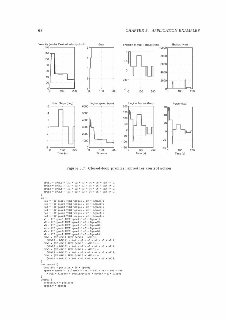
68 CHAPTER 5. APPLICATION EXAMPLES
Figure 5.7: Closed-loop profiles: smoother control action
dPWL1 = wPWL1 - (w1 + w2 + w3 + w4 + w5 + wR) <= 0;dPWL2 = wPWL2 - (w1 + w2 + w3 + w4 + w5 + wR) <= 0;dPWL3 = wPWL3 - (w1 + w2 + w3 + w4 + w5 + wR) <= 0;dPWL4 = wPWL4 - (w1 + w2 + w3 + w4 + w5 + wR) <= 0;
}DA {
Fe1 = {IF gear1 THEN torque / sf * Rgear1};Fe2 = {IF gear2 THEN torque / sf * Rgear2};Fe3 = {IF gear3 THEN torque / sf * Rgear3};Fe4 = {IF gear4 THEN torque / sf * Rgear4};Fe5 = {IF gear5 THEN torque / sf * Rgear5};FeR = {IF gearR THEN torque / sf * RgearR};w1 = {IF gear1 THEN speed / sf * Rgear1};w2 = {IF gear2 THEN speed / sf * Rgear2};w3 = {IF gear3 THEN speed / sf * Rgear3};w4 = {IF gear4 THEN speed / sf * Rgear4};w5 = {IF gear5 THEN speed / sf * Rgear5};wR = {IF gearR THEN speed / sf * RgearR};DCe1 = {IF dPWL1 THEN (aPWL2 - aPWL1) +(bPWL2 - bPWL1) * (w1 + w2 + w3 + w4 + w5 + wR)};
DCe2 = {IF dPWL2 THEN (aPWL3 - aPWL2) +(bPWL3 - bPWL2) * (w1 + w2 + w3 + w4 + w5 + wR)};
DCe3 = {IF dPWL3 THEN (aPWL4 - aPWL3) +(bPWL4 - bPWL3) * (w1 + w2 + w3 + w4 + w5 + wR)};
DCe4 = {IF dPWL4 THEN (aPWL5 - aPWL4) +(bPWL5 - bPWL4) * (w1 + w2 + w3 + w4 + w5 + wR)};
}CONTINUOUS {
position = position + Ts * speed;speed = speed + Ts / mass * (Fe1 + Fe2 + Fe3 + Fe4 + Fe5+ FeR - F_brake - beta_friction * speed) - g * slope;
}OUTPUT {
position_y = position;speed_y = speed;
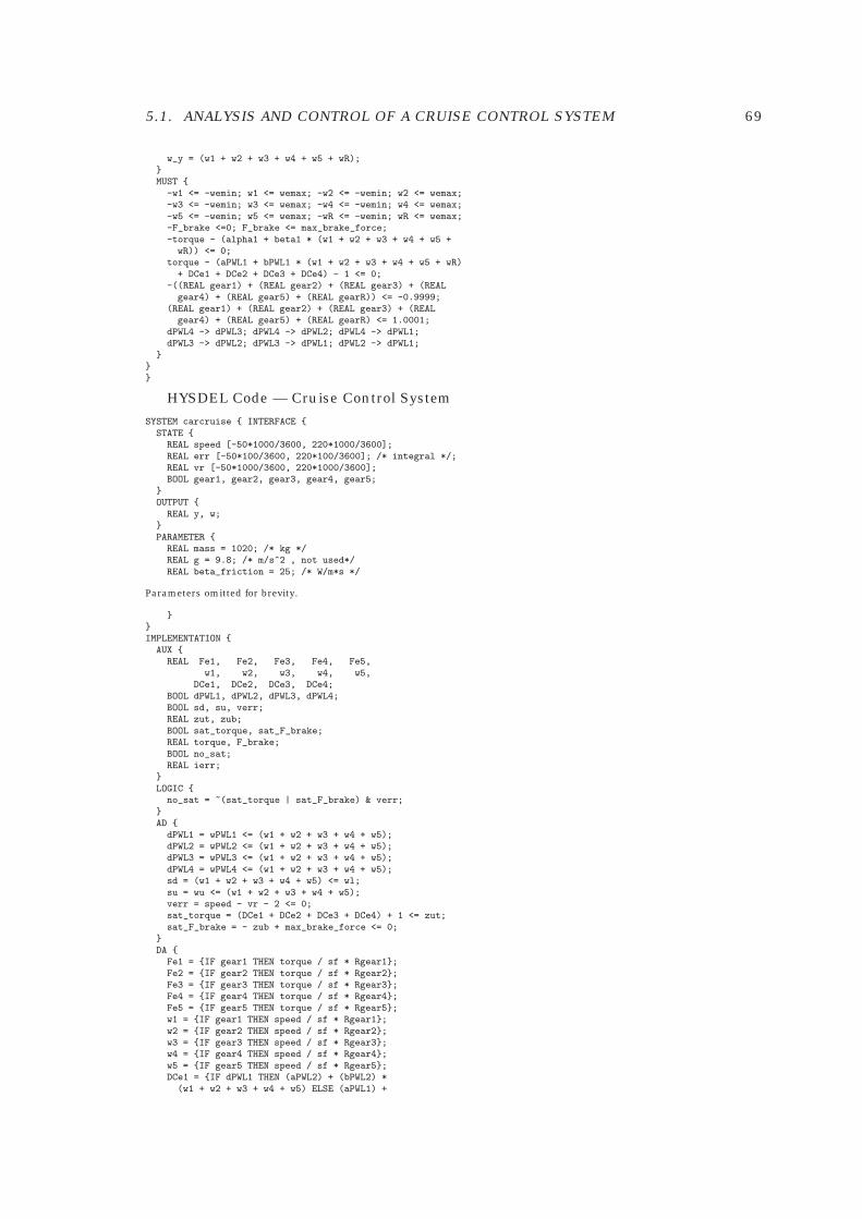
5.1. ANALYSIS AND CONTROL OF A CRUISE CONTROL SYSTEM 69
w_y = (w1 + w2 + w3 + w4 + w5 + wR);}MUST {
-w1 <= -wemin; w1 <= wemax; -w2 <= -wemin; w2 <= wemax;-w3 <= -wemin; w3 <= wemax; -w4 <= -wemin; w4 <= wemax;-w5 <= -wemin; w5 <= wemax; -wR <= -wemin; wR <= wemax;-F_brake <=0; F_brake <= max_brake_force;-torque - (alpha1 + beta1 * (w1 + w2 + w3 + w4 + w5 +wR)) <= 0;
torque - (aPWL1 + bPWL1 * (w1 + w2 + w3 + w4 + w5 + wR)+ DCe1 + DCe2 + DCe3 + DCe4) - 1 <= 0;
-((REAL gear1) + (REAL gear2) + (REAL gear3) + (REALgear4) + (REAL gear5) + (REAL gearR)) <= -0.9999;
(REAL gear1) + (REAL gear2) + (REAL gear3) + (REALgear4) + (REAL gear5) + (REAL gearR) <= 1.0001;
dPWL4 -> dPWL3; dPWL4 -> dPWL2; dPWL4 -> dPWL1;dPWL3 -> dPWL2; dPWL3 -> dPWL1; dPWL2 -> dPWL1;
}}}
HYSDEL Code — Cruise Control System
SYSTEM carcruise { INTERFACE {STATE {
REAL speed [-50*1000/3600, 220*1000/3600];REAL err [-50*100/3600, 220*100/3600]; /* integral */;REAL vr [-50*1000/3600, 220*1000/3600];BOOL gear1, gear2, gear3, gear4, gear5;
}OUTPUT {
REAL y, w;}PARAMETER {
REAL mass = 1020; /* kg */REAL g = 9.8; /* m/s^2 , not used*/REAL beta_friction = 25; /* W/m*s */
Parameters omitted for brevity.
}}IMPLEMENTATION {
AUX {REAL Fe1, Fe2, Fe3, Fe4, Fe5,
w1, w2, w3, w4, w5,DCe1, DCe2, DCe3, DCe4;
BOOL dPWL1, dPWL2, dPWL3, dPWL4;BOOL sd, su, verr;REAL zut, zub;BOOL sat_torque, sat_F_brake;REAL torque, F_brake;BOOL no_sat;REAL ierr;
}LOGIC {
no_sat = ~(sat_torque | sat_F_brake) & verr;}AD {
dPWL1 = wPWL1 <= (w1 + w2 + w3 + w4 + w5);dPWL2 = wPWL2 <= (w1 + w2 + w3 + w4 + w5);dPWL3 = wPWL3 <= (w1 + w2 + w3 + w4 + w5);dPWL4 = wPWL4 <= (w1 + w2 + w3 + w4 + w5);sd = (w1 + w2 + w3 + w4 + w5) <= wl;su = wu <= (w1 + w2 + w3 + w4 + w5);verr = speed - vr - 2 <= 0;sat_torque = (DCe1 + DCe2 + DCe3 + DCe4) + 1 <= zut;sat_F_brake = - zub + max_brake_force <= 0;
}DA {
Fe1 = {IF gear1 THEN torque / sf * Rgear1};Fe2 = {IF gear2 THEN torque / sf * Rgear2};Fe3 = {IF gear3 THEN torque / sf * Rgear3};Fe4 = {IF gear4 THEN torque / sf * Rgear4};Fe5 = {IF gear5 THEN torque / sf * Rgear5};w1 = {IF gear1 THEN speed / sf * Rgear1};w2 = {IF gear2 THEN speed / sf * Rgear2};w3 = {IF gear3 THEN speed / sf * Rgear3};w4 = {IF gear4 THEN speed / sf * Rgear4};w5 = {IF gear5 THEN speed / sf * Rgear5};DCe1 = {IF dPWL1 THEN (aPWL2) + (bPWL2) *(w1 + w2 + w3 + w4 + w5) ELSE (aPWL1) +
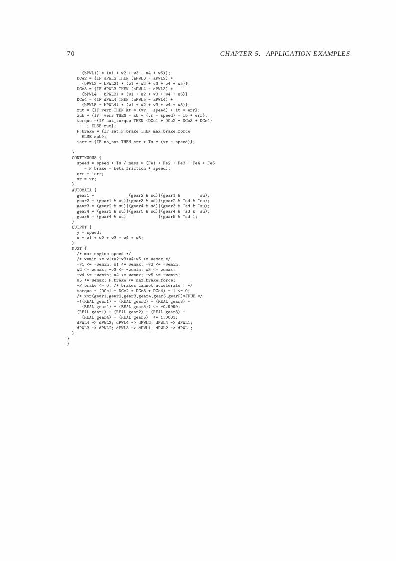
70 CHAPTER 5. APPLICATION EXAMPLES
(bPWL1) * (w1 + w2 + w3 + w4 + w5)};DCe2 = {IF dPWL2 THEN (aPWL3 - aPWL2) +(bPWL3 - bPWL2) * (w1 + w2 + w3 + w4 + w5)};
DCe3 = {IF dPWL3 THEN (aPWL4 - aPWL3) +(bPWL4 - bPWL3) * (w1 + w2 + w3 + w4 + w5)};
DCe4 = {IF dPWL4 THEN (aPWL5 - aPWL4) +(bPWL5 - bPWL4) * (w1 + w2 + w3 + w4 + w5)};
zut = {IF verr THEN kt * (vr - speed) + it * err};zub = {IF ~verr THEN - kb * (vr - speed) - ib * err};torque ={IF sat_torque THEN (DCe1 + DCe2 + DCe3 + DCe4)+ 1 ELSE zut};
F_brake = {IF sat_F_brake THEN max_brake_forceELSE zub};
ierr = {IF no_sat THEN err + Ts * (vr - speed)};
}CONTINUOUS {
speed = speed + Ts / mass * (Fe1 + Fe2 + Fe3 + Fe4 + Fe5- F_brake - beta_friction * speed);
err = ierr;vr = vr;
}AUTOMATA {
gear1 = (gear2 & sd)|(gear1 & ~su);gear2 = (gear1 & su)|(gear3 & sd)|(gear2 & ~sd & ~su);gear3 = (gear2 & su)|(gear4 & sd)|(gear3 & ~sd & ~su);gear4 = (gear3 & su)|(gear5 & sd)|(gear4 & ~sd & ~su);gear5 = (gear4 & su) |(gear5 & ~sd );
}OUTPUT {
y = speed;w = w1 + w2 + w3 + w4 + w5;
}MUST {
/* max engine speed *//* wemin <= w1+w2+w3+w4+w5 <= wemax */-w1 <= -wemin; w1 <= wemax; -w2 <= -wemin;w2 <= wemax; -w3 <= -wemin; w3 <= wemax;-w4 <= -wemin; w4 <= wemax; -w5 <= -wemin;w5 <= wemax; F_brake <= max_brake_force;-F_brake <= 0; /* brakes cannot accelerate ! */torque - (DCe1 + DCe2 + DCe3 + DCe4) - 1 <= 0;/* xor(gear1,gear2,gear3,gear4,gear5,gearR)=TRUE */-((REAL gear1) + (REAL gear2) + (REAL gear3) +(REAL gear4) + (REAL gear5)) <= -0.9999;
(REAL gear1) + (REAL gear2) + (REAL gear3) +(REAL gear4) + (REAL gear5) <= 1.0001;
dPWL4 -> dPWL3; dPWL4 -> dPWL2; dPWL4 -> dPWL1;dPWL3 -> dPWL2; dPWL3 -> dPWL1; dPWL2 -> dPWL1;
}}}
Chapter 6
Conclusions
We introduced Discrete Hybrid Automata as a general modeling framework for obtain-ing hybrid models oriented to the solution of analysis and synthesis problems. Thelanguage HYSDEL describes DHA at a high level and its associated compiler generatesthe corresponding computational models. This simplifies the use of the whole theoryand set of tools available for different classes of hybrid systems for solving control, stateestimation and verification problems. The effectiveness of HYSDEL was shown on anautomotive case study.
HYSDEL has been successfully used in several industrial applications. In [40] theauthors modeled the hybrid behavior of a vehicle/tyre system and designed a tractioncontroller that improves a driver’s ability to control a vehicle under adverse externalconditions such as wet or icy roads. Another automotive application was presentedin [22], where the focus is on the application of hybrid modeling and optimal control tothe problem of air-to-fuel ratio and torque control in advanced gasoline direct injectionstratified charge (DISC) engines. In both cases, the control design leaded to a controllaw that can be implemented on automotive hardware as a piecewise affine function ofthe measured and estimated quantities. In [70] the economic optimization of a com-bined cycle power plant was accomplished by modeling the system in HYSDEL (turningon/off the gas and steam turbine, operating constraints, different modalities start upof the turbines), and then using the generated MLD model in a mixed integer linearoptimization algorithm [92].
The HYSDEL compiler is available on-line at http://control.ee.ethz.ch/~hybrid/hysdel.
Acknowledgments
Most of the contents of these notes is based on papers that I published with severalcoauthors. I am thankful to all of them, and especially to Fabio Torrisi and FrancescoBorrelli.
71

72 CHAPTER 6. CONCLUSIONS
Bibliography
[1] J. Acevedo and E.N. Pistikopoulos. A multiparametric programming approach forlinear process engineering problems under uncertainty. Ind. Eng. Chem. Res.,36:717–728, 1997.
[2] R. Alur, C. Belta, F. Ivancic, V. Kumar, M. Mintz, G.J. Pappas, H. Rubin, andJ. Schug. Hybrid modeling and simulation of biomolecular networks. In M.D. DiBenedetto and A. Sangiovanni Vincentelli, editors, Hybrid Systems: Computationand Control, volume 2034 of Lecture Notes in Computer Science, pages 19–33.Springer-Verlag, 2001.
[3] R. Alur, C. Courcoubetis, T.A. Henzinger, and P.-H. Ho. Hybrid automata: Analgorithmic approach to the specification and verification of hybrid systems. InA.P. Ravn R.L. Grossman, A. Nerode and H. Rischel, editors, Hybrid Systems,volume 736 of Lecture Notes in Computer Science, pages 209–229. Springer-Verlag,1993.
[4] P.J. Antsaklis. A brief introduction to the theory and applications of hybrid sys-tems. Proc. IEEE, Special Issue on Hybrid Systems: Theory and Applications,88(7):879–886, July 2000.
[5] A. Asarin, O. Maler, and A. Pnueli. On the analysis of dynamical systems havingpiecewise-constant derivatives. Theoretical Computer Science, 138:35–65, 1995.
[6] E. Asarin, O. Bournez, T. Dang, and O. Maler. Reachability analysis of piecewise-linear dynamical systems. In B. Krogh and N. Lynch, editors, Hybrid Systems:Computation and Control, volume 1790 of Lecture Notes in Computer Science, pages20–31. Springer-Verlag, 2000.
[7] E. Asarin, M. Bozga, A. Kerbrat, O. Maler, A. Pnueli, and A. Rasse. Data-structuresfor the verification of timed automata. In O. Maler, editor, Hybrid and Real-Time Systems, volume 1201 of Lecture notes in Computer Science, pages 346–360.Springer-Verlag, 1997.
[8] D. Avis, D. Bremmer, and R. Seidel. How good are convex hull algorithms? Com-putational Geometry: Theory and Applications, 7:265–301, 1997.
[9] A. Balluchi, M. Di Benedetto, C. Pinello, C. Rossi, and A. Sangiovanni-Vincentelli.Hybrid control for automotive engine management: the cut-off case. In T.A. Hen-zinger and S. Sastry, editors, Hybrid Systems: Computation and Control, volume1386 of Lecture Notes in Computer Science, pages 13–32. Springer-Verlag, 1998.
[10] A. Balluchi, L. Benvenuti, M. Di Benedetto, C. Pinello, and A. Sangiovanni-Vincentelli. Automotive engine control and hybrid systems: Challenges and op-portunities. Proc. IEEE, 88(7):888–912, 2000.
73
74 BIBLIOGRAPHY
[11] G. Behrmann, A. Fehnker, T. Hune, K. Larsen, P. Pettersson, J. Romijn, andF. Vaandrager. Minimum-cost reachability for priced timed automata. In M.D. DiBenedetto and A. Sangiovanni Vincentelli, editors, Hybrid Systems: Computationand Control, volume 2034 of Lecture Notes in Computer Science, pages 147–162.Springer-Verlag, 2001.
[12] A. Bemporad. Identification of hybrid systems: Global convergence via mixed-integer programming. Technical Report AUT00-28, ETH, Zurich, September 2000.
[13] A. Bemporad. An efficient technique for translating mixed logical dynamical sys-tems into piecewise affine systems. In Proc. 41th IEEE Conf. on Decision and Con-trol, pages 1970–1975, 2002.
[14] A. Bemporad, P. Borodani, and M. Mannelli. Hybrid control of an automotiverobotized gearbox for reduction of consumptions and emissions. In O. Maler andA. Pnueli, editors, Hybrid Systems: Computation and Control, number 2623 inLecture Notes in Computer Science, pages 81–96. Springer-Verlag, 2003.
[15] A. Bemporad, F. Borrelli, and M. Morari. Optimal controllers for hybrid systems:Stability and piecewise linear explicit form. In Proc. 39th IEEE Conf. on Decisionand Control, pages 1810–1815, Sydney, Australia, December 2000.
[16] A. Bemporad, F. Borrelli, and M. Morari. Piecewise linear optimal controllers forhybrid systems. In American Control Conference, pages 1190–1194, Chicago, IL,June 2000.
[17] A. Bemporad, F. Borrelli, and M. Morari. On the optimal control law for lineardiscrete time hybrid systems. In M. Greenstreet and C. Tomlin, editors, HybridSystems: Computation and Control, number 2289 in Lecture Notes in ComputerScience, pages 105–119. Springer-Verlag, 2002.
[18] A. Bemporad, G. Ferrari-Trecate, and M. Morari. Observability and controlla-bility of piecewise affine and hybrid systems. IEEE Trans. Automatic Control,45(10):1864–1876, 2000.
[19] A. Bemporad, C. Filippi, and F.D. Torrisi. Inner and outer approximation of poly-topes using boxes. Computational Geometry, 2002. Submitted for publication.
[20] A. Bemporad, A. Garulli, S. Paoletti, and A. Vicino. A greedy approach to iden-tification of piecewise affine models. In O. Maler and A. Pnueli, editors, HybridSystems: Computation and Control, number 2623 in Lecture Notes in ComputerScience, pages 97–112. Springer-Verlag, 2003.
[21] A. Bemporad, A. Garulli, S. Paoletti, and A. Vicino. Set membership identificationof piecewise affine models. In 13th IFAC Symposium on System Identification,Rotterdam, The Netherlands, August 2003.
[22] A. Bemporad, N. Giorgetti, I.V. Kolmanovsky, and D. Hrovat. Hybrid modeling andcontrol of a direct injection stratified charge engine. In HSCC’02.
[23] A. Bemporad, N. Giorgetti, I.V. Kolmanovsky, and D. Hrovat. Hybrid model-ing and control of a direct injection stratified charge engine. In Symposium onAdvanced Automotive Technologies, ASME International Mechanical EngineeringCongress and Exposition, New Orleans, Louisiana, November 2002.
[24] A. Bemporad, N. Giorgetti, I.V. Kolmanovsky, and D. Hrovat. A hybrid systemapproach to modeling and optimal control of DISC engines. In Proc. 41th IEEEConf. on Decision and Control, pages 1582–1587, 2002.
BIBLIOGRAPHY 75
[25] A. Bemporad, L. Giovanardi, and F.D. Torrisi. Performance driven reachabilityanalysis for optimal scheduling and control of hybrid systems. Technical ReportAUT00-15, Automatic Control Laboratory, ETH Zurich, Switzerland, September2000. To be submitted.
[26] A. Bemporad, L. Giovanardi, and F.D. Torrisi. Performance driven reachabilityanalysis for optimal scheduling and control of hybrid systems. In Proc. 39th IEEEConf. on Decision and Control, pages 969–974, Sydney, Australia, December 2000.
[27] A. Bemporad, A. Giua, and C. Seatzu. Synthesis of state-feedback optimal con-trollers for switched linear systems. In Proc. 41th IEEE Conf. on Decision andControl, pages 3182–3187, 2002.
[28] A. Bemporad, W.P.M.H. Heemels, and B. De Schutter. On hybrid systems andclosed-loop MPC systems. IEEE Trans. Automatic Control, 47(5):863–869, May2002.
[29] A. Bemporad and D. Mignone. MIQP.M: A Matlab function for solving mixed integerquadratic programs. ETH Zurich, 2000. See related web page at http://www.dii.unisi.it/~hybrid/tools/miqp. Code also available at http://control.ethz.ch/~hybrid/miqp.
[30] A. Bemporad, D. Mignone, and M. Morari. Moving horizon estimation for hybridsystems and fault detection. In American Control Conference, pages 2471–2475,Chicago, IL, June 1999.
[31] A. Bemporad and M. Morari. Control of systems integrating logic, dynamics, andconstraints. Automatica, 35(3):407–427, March 1999.
[32] A. Bemporad and M. Morari. Verification of hybrid systems via mathematical pro-gramming. In F.W. Vaandrager and J.H. van Schuppen, editors, Hybrid Systems:Computation and Control, volume 1569 of Lecture Notes in Computer Science, pages31–45. Springer-Verlag, 1999.
[33] A. Bemporad, M. Morari, V. Dua, and E.N. Pistikopoulos. The explicit linearquadratic regulator for constrained systems. Automatica, 38(1):3–20, 2002.
[34] A. Bemporad, J. Roll, and L. Ljung. Identification of hybrid systems via mixed-integer programming. Technical Report AUT00-29, ETH, Zurich, October 2000.
[35] A. Bemporad, F.D. Torrisi, and M. Morari. Optimization-based verification andstability characterization of piecewise affine and hybrid systems. In B. Kroghand N. Lynch, editors, Hybrid Systems: Computation and Control, volume 1790 ofLecture Notes in Computer Science, pages 45–58. Springer-Verlag, 2000.
[36] A. Bemporad, F.D. Torrisi, and M. Morari. Performance analysis of piecewiselinear systems and model predictive control systems. In Proc. 39th IEEE Conf. onDecision and Control, pages 4957–4962, Sydney, Australia, December 2000.
[37] A. Bemporad, F.D. Torrisi, and M. Morari. Discrete-time hybrid modeling and ver-ification of the batch evaporator process benchmark. European Journal of Control,7(4):382–399, July 2001.
[38] Johan Bengtsson, Kim G. Larsen, Fredrik Larsson, Paul Pettersson, Yi Wang, andCarsten Weise. New Generation of UPPAAL. In Int. Workshop on Software Tools forTechnology Transfer, June 1998.
[39] F. Borrelli, M. Baotic, A. Bemporad, and M. Morari. An efficient algorithm forcomputing the state feedback optimal control law for discrete time hybrid systems.In American Control Conference, Denver, Colorado, 2003.
76 BIBLIOGRAPHY
[40] F. Borrelli, A. Bemporad, M. Fodor, and D. Hrovat. A hybrid approach to tractioncontrol. In A. Sangiovanni-Vincentelli and M.D. Di Benedetto, editors, HybridSystems: Computation and Control, number 2034 in Lecture Notes in ComputerScience, pages 162–174. Springer-Verlag, 2001.
[41] F. Borrelli, A. Bemporad, and M. Morari. A geometric algorithm for multi-parametric linear programming. Journal of Optimization Theory and Applications,2002. Accepted for publication as a regular paper.
[42] R. Bosch. Automotive Handbook. Society of Automotive Engineers, 5 edition,December 2000.
[43] O. Botchkarev and S. Tripakis. Verification of hybrid systems with linear differ-ential inclusions using ellipsoidal approximations. In B. Krogh and N. Lynch,editors, Hybrid Systems: Computation and Control, volume 1790 of Lecture Notesin Computer Science, pages 73–88. Springer-Verlag, 2000.
[44] M.S. Branicky. Studies in hybrid systems: modeling, analysis, and control. PhDthesis, LIDS-TH 2304, Massachusetts Institute of Technology, Cambridge, MA,1995.
[45] M.S. Branicky. Multiple Lyapunov functions and other analysis tools for switchedand hybrid systems. IEEE Trans. Automatic Control, 43(4):475–482, April 1998.
[46] M.S. Branicky, V.S. Borkar, and S.K. Mitter. A unified framework for hybrid con-trol: model and optimal control theory. IEEE Trans. Automatic Control, 43(1):31–45, 1998.
[47] M.S. Branicky and S.K. Mitter. Algorithms for optimal hybrid control. In Proc.34th IEEE Conf. on Decision and Control, New Orleans, USA, December 1995.
[48] P.J. Campo and M. Morari. Robust model predictive control. In American ControlConference, volume 2, pages 1021–1026, 1987.
[49] C. G. Cassandras and S. Lafortune. Introduction to Discrete Event Systems. KluwerAcademic Publishers, 1999.
[50] C. G. Cassandras, Q. Liu, K. Gokbayrak, and D.L. Pepyne. Optimal control ofa two-stage hybrid manufacturing system model. In Proc. 38th IEEE Conf. onDecision and Control, pages 450–455, Phoenix, AZ, December 1999.
[51] C.G. Cassandras, D.L. Pepyne, and Y.Wardi. Optimal control of a class of hybridsystems. IEEE Trans. Automatic Control, 46(3):3981–415, 2001.
[52] T.M. Cavalier, P.M. Pardalos, and A.L. Soyster. Modeling and integer programmingtechniques applied to propositional calculus. Computers Opns Res., 17(6):561–570, 1990.
[53] M.K. Camlıbel, W.P.M.H. Heemels, and J.M. Schumacher. Consistency of a time-stepping method for a class of piecewise linear networks. IEEE Trans. CircuitsSyst. I, 49(3):349–357, 2002.
[54] V. Chandru and J.N. Hooker. Optimization methods for logical inference. Wiley-Interscience, 1999.
[55] D. Christiansen. Electronics Engineers’ Handbook, 4th edition. IEEE Press/ Mc-Graw Hill, Inc., 1997.
[56] A. Chutinan and B.H. Krogh. Verification of infinite-state dynamic systems us-ing approximate quotient transition systems. IEEE Trans. Automatic Control,46(9):1401–1410, 2001.
BIBLIOGRAPHY 77
[57] A. Chutinan and B.H. Krogh. Computational techniques for hybrid system verifi-cation. IEEE Trans. Automatic Control, 48(1):64–75, 2003.
[58] E. M. Clarke, E. A. Emerson, and A. P. Sistla. Automatic verification of finite-state concurrent systems using temporal logic specifications. ACM Transactionson Programming Languages and Systems, 8(2):244–263, 1986.
[59] F.A. Cuzzola and M. Morari. A generalized approach for analysis and control ofdiscrete-time piecewise affine and hybrid systems. In A. Sangiovanni-Vincentelliand M.D. Di Benedetto, editors, Hybrid Systems: Computation and Control, num-ber 2034 in Lecture Notes in Computer Science, pages 189–203. Springer-Verlag,2001.
[60] T. Dang and O. Maler. Reachability analysis via face lifting. In T.A. Henzingerand S. Sastry, editors, Hybrid Systems: Computation and Control, volume 1386 ofLecture Notes in Computer Science, pages 96–109. Springer-Verlag, 1998.
[61] Dash Associates. XPRESS-MP User Guide, 2003. http://www.dashopt.com.
[62] B. De Schutter. Optimal control of a class of linear hybrid systems with satura-tion. SIAM J. Control Optim., 39(3):835–851, 2000.
[63] B. De Schutter and B. De Moor. The extended linear complementarity problem andthe modeling and analysis of hybrid systems. In P. Antsaklis, W. Kohn, M. Lem-mon, A. Nerode, and S. Sastry, editors, Hybrid Systems V, volume 1567 of LectureNotes in Computer Science, pages 70–85. Springer, 1999.
[64] B. De Schutter and T. van den Boom. Model predictive control for max-plus-linearsystems. In American Control Conference, pages 4046–4050, 2000.
[65] B. De Schutter and T. van den Boom. On model predictive control for max-min-plus-scaling discrete event systems. Technical Report bds:00-04, Control Labora-tory, Fac. of Information Technology and Systems, Delft University of Technology,Delft, The Netherlands, February 2000.
[66] D. Dill. Timing assumptions and verification of finite-state concurrent systems.In R.L. Grossman, A. Nerode, A.P. Ravn, and H. Rischel, editors, Proc. of theWorkshop Automatic Verification Methods for Finite State Systems, volume 407 ofLecture Notes in Computer Science, pages 197–212. Springer-Verlag, 1989.
[67] V.D. Dimitriadis, N. Shah, and C.C. Pantelides. Modeling and safety verificationof discrete/continuous processing systems. AIChE Journal, 43:1041–1059, 1997.
[68] V. Dua and E.N. Pistikopoulos. An algorithm for the solution of multiparamet-ric mixed integer linear programming problems. Annals of Operations Research,pages 123–139, 2000.
[69] G. Ferrari-Trecate, F.A. Cuzzola, D. Mignone, and M. Morari. Analysis of discrete-time piecewise affine and hybrid systems. Automatica, 38:2139–2146, 2002.
[70] G. Ferrari-Trecate, E. Gallestey, P. Letizia, M. Spedicato, M. Morari, and M. An-toine. Modeling and control of co-generation power plants: A hybrid system ap-proach. In C. J. Tomlin and M. R. Greenstreet, editors, Hybrid Systems: Com-putation and Control, volume 2289 of Lecture Notes in Computer Science, pages209–224. Springer-Verlag, 2002.
[71] G. Ferrari-Trecate, D. Mignone, and M. Morari. Moving horizon estimation forhybrid systems. IEEE Trans. Automatic Control, 47(10):1663–1676, 2002.
78 BIBLIOGRAPHY
[72] G. Ferrari-Trecate, M. Muselli, D. Liberati, and M. Morari. A clustering techniquefor the identification of piecewise affine systems. In A. Sangiovanni-Vincentelli andM.D. Di Benedetto, editors, Hybrid Systems: Computation and Control, LectureNotes in Computer Science. Springer-Verlag, 2001.
[73] G. Ferrari-Trecate, M. Muselli, D. Liberati, and M. Morari. A clustering tech-nique for the identification of piecewise affine systems. Automatica, 39(2):205–217, February 2003.
[74] J.A. Ferrez, K. Fukuda, and T.M. Liebling. Cuts, zonotopes and arrangements.Technical report, EPF Lausanne, Switzerland, November 2001.
[75] R. Fletcher and S. Leyffer. Numerical experience with lower bounds for MIQPbranch-and-bound. SIAM J. Optim., 8(2):604–616, May 1998.
[76] C. A. Floudas. Nonlinear and Mixed-Integer Optimization. Oxford University Press,1995.
[77] K. Fukuda. cdd/cdd+ Reference Manual. Institute for Operations Research, ETH-Zentrum, CH-8092 Zurich, Switzerland, 0.61 (cdd) 0.75 (cdd+) edition, December1997.
[78] K. Fukuda. From the zonotope construction to the minkowski addition of convexpolytopes. Technical report, Preprint, School of Computer Scince, McGill Univer-sity, Montreal, Canada, August 2003.
[79] T. Geyer, F.D. Torrisi, and M. Morari. Efficient Mode Enumeration of Composi-tional Hybrid Models. In A. Pnueli and O. Maler, editors, Hybrid Systems: Compu-tation and Control, Lecture Notes in Computer Science. Springer-Verlag, 2003.
[80] E.G. Gilbert and K. Tin Tan. Linear systems with state and control constraints:the theory and applications of maximal output admissible sets. IEEE Trans. Auto-matic Control, 36(9):1008–1020, 1991.
[81] F. Glover. Improved linear integer programming formulations of nonlinear integerproblems. Management Science, 22(4):455–460, 1975.
[82] K. Gokbayrak and C.G. Cassandras. A hierarchical decomposition method for op-timal control of hybrid systems. In Proc. 38th IEEE Conf. on Decision and Control,pages 1816–1821, Phoenix, AZ, December 1999.
[83] P. Gritzmann and V. Klee. On the complexity of some basic problems in compu-tational convexity: I. Containment problems. Discrete Mathematics, 136:129–174,1994.
[84] P. Gritzmann and B. Sturmfels. Minkowsky addition of polytopes: Computationalcomplexity and applications to Grobner bases. SIAM Journal on Discrete Mathe-matics, 6(2):246–269, May 1993.
[85] S. Hedlund and A. Rantzer. Optimal control of hybrid systems. In Proc. 38th IEEEConf. on Decision and Control, pages 3972–3976, Phoenix, AZ, December 1999.
[86] W.P.H.M Heemels, B. de Schutter, and A. Bemporad. On the equivalence of classesof hybrid dynamical models. In Proc. 40th IEEE Conf. on Decision and Control,pages 364–369, Orlando, Florida, 2001.
[87] W.P.M.H. Heemels. Linear complementarity systems: a study in hybrid dynamics.PhD thesis, Dept. of Electrical Engineering, Eindhoven University of Technology,The Netherlands, 1999.
BIBLIOGRAPHY 79
[88] W.P.M.H. Heemels, J.M. Schumacher, and S. Weiland. Linear complementaritysystems. SIAM Journal on Applied Mathematics, 60(4):1234–1269, 2000.
[89] T.A. Henzinger, B. Horowitz, R. Majumdar, and H. Wong-Toi. Beyond HyTech:Hybrid systems analysis using interval numerical methods. In B. Krogh andN. Lynch, editors, Hybrid Systems: Computation and Control, volume 1790 ofLecture Notes in Computer Science, pages 130–144. Springer-Verlag, 2000.
[90] J. P. Hespanha, S. Bohacek, K. Obraczka, and J. Lee. Hybrid modeling of TCPcongestion control. In M.D. Di Benedetto and A. Sangiovanni Vincentelli, edi-tors, Hybrid Systems: Computation and Control, volume 2034 of Lecture Notes inComputer Science, pages 291–304. Springer-Verlag, 2001.
[91] T. Huerlimann. Reference Manual for the LPL Modeling Language, Version 4.42. De-partement for Informatics, Universite de Fribourg, Switzerland, http://www2-iiuf.unifr.ch/tcs/lpl/TonyHome.htm, 2001.
[92] ILOG, Inc. CPLEX 8.1 User Manual. Gentilly Cedex, France, 2003.
[93] M. Johannson and A. Rantzer. Computation of piece-wise quadratic Lyapunovfunctions for hybrid systems. IEEE Trans. Automatic Control, 43(4):555–559,1998.
[94] T.A. Johansen, J. Kalkkuhl, J. Ludemann, and I. Petersen. Hybrid control strate-gies in ABS. In American Control Conference, Arlington, Virginia, June 2001.
[95] K H Johansson, M Egerstedt, J Lygeros, and S Sastry. On the regularization ofZeno hybrid automata. System & Control Letters, 38:141–150, 1999.
[96] P. Julian. A High Level Canonical Piecewise Linear Representation: Theory andApplications. Phd thesis, Universidad National del Sur, Bah/’ıa Blanca, 1999.
[97] P. Julian, M. Jordan, and A. Desages. Canonical piecewise-linear approximationof smooth functions. IEEE Trans. Circuits and Systems — I: Fundamental Theoryand Applications, 45(5):567–571, May 1998.
[98] I. Kolmanovsky and E.G. Gilbert. Theory and computation of disturbance invari-ant sets for discrete-time linear systems. Mathematical Problems in Engineering,4:317–367, 1998.
[99] A. B. Kurzhanski and P. Varaiya. Ellipsoidal techniques for reachability analysis.In B. Krogh and N. Lynch, editors, Hybrid Systems: Computation and Control, vol-ume 1790 of Lecture Notes in Computer Science, pages 202–214. Springer-Verlag,2000.
[100] B. Lincoln and A. Rantzer. Optimizing linear system switching. In Proc. 40th IEEEConf. on Decision and Control, pages 2063–2068, Orlando, FL, USA, 2001.
[101] J. Lygeros, D.N. Godbole, and S. Sastry. A game theoretic approach to hybridsystem design. In R. Alur and T. Henzinger, editors, Hybrid Systems III, volume1066 of Lecture Notes in Computer Science, pages 1–12. Springer-Verlag, 1996.
[102] J. Lygeros, K.H. Johansson, S.N. Simic, J. Zhang, and S.S. Sastry. Dynamicalproperties of hybrid automata. IEEE Trans. Automatic Control, 48:2–17, January2003.
[103] J. Lygeros, C. Tomlin, and S. Sastry. Controllers for reachability specifications forhybrid systems. Automatica, 35(3):349–370, 1999.
[104] A. Makhorin. GLPK (GNU Linear Programming Kit) User’s Guide, 2003.
80 BIBLIOGRAPHY
[105] F. Martinelli. A scheduling problem for n competing queues with finite capacity.In Proc. 38th IEEE Conf. on Decision and Control, pages 2276–2281, Phoenix, AZ,December 1999.
[106] D.Q. Mayne, J.B. Rawlings, C.V. Rao, and P.O.M. Scokaert. Constrained modelpredictive control: Stability and optimality. Automatica, 36(6):789–814, June2000.
[107] D. Mignone. Control and Estimation of Hybrid Systems with Mathematical Opti-mization. PhD thesis, Automatic Control Labotatory - ETH, Zurich, 2002.
[108] D. Mignone, G. Ferrari-Trecate, and M. Morari. Stability and stabilization of piece-wise affine and hybrid systems: An LMI approach. In Proc. 39th IEEE Conf. onDecision and Control, pages 504–509, December 2000.
[109] G. Mitra, C. Lucas, and Moody S. Tool for reformulating logical forms into zero-onemixed integer programs. European Journal of Operational Research, 71:262–276,1994.
[110] R. Mobus, M. Baotic, and M. Morari. Multi-objective adaptive cruise control. InHSCC’03, Prague, The Czech Republic, April 2003. Accepted.
[111] M. Morari, A. Bemporad, and D. Mignone. A framework for control, state estima-tion, fault detection, and verification of hybrid systems. Automatisierungstechnik,47:374–381, 1999.
[112] G.L. Nemhauser and L.A. Wolsey. Integer and Combinatorial Optimization. Wiley,1988.
[113] Th. Ottmann, S. Schuierer, and S. Soundaralakshmi. Enumerating extremepoints in higher dimensions. In E.W. Mayer and C. Puech, editors, STACS 95:12th Annual Symposium on Theoretical Aspects of Computer Science, Lecture Notesin Computer Science 900, pages 562–570. Springer-Verlag, 1995.
[114] C.C. Pantelides, M.P. Avraam, and N. Shah. Optimisation of hybrid dynamic pro-cesses. In F. Keil, W. Mackens, H. Voss, and J. Werther, editors, Scientific Com-puting in Chemical Engineering, pages 62–76. Springer-Verlag, 1999.
[115] T. Park and P.I. Barton. Implicit model checking of logic-based control systems.AIChE Journal, 43(9):2246–2260, 1997.
[116] B. Piccoli. Necessary conditions for hybrid optimization. In Proc. 38th IEEE Conf.on Decision and Control, Phoenix, Arizona USA, December 1999.
[117] B. Potocnik, A. Bemporad, F.D. Torrisi, G. Music, and B. Zupancic. Schedulingof hybrid systems: Multi product batch plant. In Proc. IFAC World Congress,Barcelona, 2002.
[118] S.J. Qin and T.A. Badgwell. An overview of industrial model predictive controltechnology. In Chemical Process Control - V, volume 93, no. 316, pages 232–256.AIChe Symposium Series - American Institute of Chemical Engineers, 1997.
[119] R. Raman and I.E. Grossmann. Relation between MILP modeling and logical in-ference for chemical process synthesis. Computers Chem. Engng., 15(2):73–84,1991.
[120] A. Rantzer and M. Johansson. Piecewise linear quadratic optimal control. InAmerican Control Conference, pages 1749–1753, Albuquerque, 1997.
BIBLIOGRAPHY 81
[121] A. Rantzer and M. Johansson. Piecewise linear quadratic optimal control. IEEETrans. Automatic Control, 45(4):629–637, April 2000.
[122] P. Riedinger, F.Kratz, C. Iung, and C.Zanne. Linear quadratic optimization forhybrid systems. In Proc. 38th IEEE Conf. on Decision and Control, Phoenix, ArizonaUSA, December 1999.
[123] J. Roll, A. Bemporad, and L. Ljung. Identification of piecewise affine systemsvia mixed-integer programming. Automatica, 2002. Conditionally accepted forpublication as a regular paper.
[124] V. A. Roschchin, O.V. Volkovich, and I.V. Sergienko. Models and methods of solu-tion of quadratic integer programming problems. Cybernetics, 23:289–305, 1987.
[125] N. V. Sahinidis. BARON — Branch And Reduce Optimization Navigator. Technicalreport, University of Illinois at Urbana-Champaign, Dept. of Chemical Engineer-ing, Urbana, IL, USA, 2000.
[126] A.J. van der Schaft and J.M. Schumacher. An Introduction to Hybrid Dynam-ical Systems, volume 251 of Lecture Notes in Control and Information Sciences.Springer, London, 2000.
[127] B.I. Silva, O. Stursberg, B.H. Krogh, and S. Engell. An assessment of the currentstatus of algorithmic approaches to the verification of hybrid systems. In Proc.40th IEEE Conf. on Decision and Control, pages 2867–2874, Orlando, Florida, De-cember 2001.
[128] E.D. Sontag. Nonlinear regulation: The piecewise linear approach. IEEE Trans.Automatic Control, 26(2):346–358, April 1981.
[129] H.J. Sussmann. A maximum principle for hybrid optimal control problems. InProc. 38th IEEE Conf. on Decision and Control, Phoenix, Arizona USA, December1999.
[130] F. Torrisi, A. Bemporad, G. Bertini, P. Hertach, D. Jost, and Mignone D. Hysdel2.0.5 - user manual. Technical Report AUT02-28, Automatic Control Laboratory,ETH Zurich, 2002.
[131] F.D. Torrisi and A. Bemporad. HYSDEL — A tool for generating computationalhybrid models. IEEE Transactions on Control Systems Technology, 2002. Acceptedfor publication. http://control.ethz.ch/~hybrid/hysdel.
[132] F.D. Torrisi, A. Bemporad, and L. Giovanardi. Reach-set computation for analysisand optimal control of discrete hybrid automata. Technical report, AutomaticControl Laboratory, ETH Zurich, 2003.
[133] M.L. Tyler and M. Morari. Propositional logic in control and monitoring problems.Automatica, 35(4):565–582, 1999.
[134] A.J. van der Schaft and J.M. Schumacher. Complementarity modelling of hybridsystems. IEEE Trans. Automatic Control, 43:483–490, 1998.
[135] H.P. Williams. Logical problems and integer programming. Bulletin of the Instituteof Mathematics and Its Applications, 13:18–20, 1977.
[136] H.P. Williams. Model Building in Mathematical Programming. John Wiley & Sons,Third Edition, 1993.
[137] H. Witsenhausen. A class of hybrid-state continuous-time dynamic systems. IEEETrans. Automatic Control, 11(2):161–167, 1966.

82 BIBLIOGRAPHY
[138] X. Xu and P.J. Antsaklis. An approach to switched systems optimal control basedon parameterization of the switching instants. In Proc. IFAC World Congress,Barcelona, Spain, 2002.
[139] X. Xu and P.J. Antsaklis. Results and perspectives on computational methods foroptimal control of switched systems. In O. Maler and A. Pnueli, editors, HybridSystems: Computation and Control, number 2623 in Lecture Notes in ComputerScience, pages 540–555. Springer-Verlag, 2003.
[140] S. Yovine. KRONOS: A verification tool for real-time systems. Software Tools forTechnology Transfer, 1(1–2):123–133, October 1997.
[141] G. M. Ziegler. Lectures on Polytopes, volume 152 of Graduate Texts in Mathematics.Springer, New York, 1994.


![Reachability Analysis for Controlled Discrete Time ...50 S. Amin et al. Reachability analysis for stochastic hybrid systems has been a recent focus of research, e.g., in [1,2,3,4]](https://img.dokumen.tips/doc/110x75/5f3f5f0cc5abeb53783e5158/reachability-analysis-for-controlled-discrete-time-50-s-amin-et-al-reachability.jpg)