Embed Size (px)
Citation preview
Modeling And Analysis Of A Cantilever Beam Tip Mass System
Vamsi C. Meesala
Thesis submitted to the Faculty of theVirginia Polytechnic Institute and State University
in partial fulfillment of the requirements for the degree of
Master of Sciencein
Engineering Mechanics
Muhammad R. Hajj, ChairSaad A. RagabShima Shahab
25th of April, 2018Blacksburg, Virginia
Keywords: Parametric excitation, Cantilever beam mass systems, Boundary conditions,Perturbation methods, Method of multiple scales, Sensitivity analysis, Uncertainty
quantification, Mass/gas sensing, Damage detection, Energy harvesting, Piezoelectricmaterials, Nonlinear constitutive relation, Parameter identification.
Copyright 2018, Vamsi C. Meesala
Modeling And Analysis Of A Cantilever Beam Tip Mass System
Vamsi C. Meesala
ABSTRACT
We model the nonlinear dynamics of a cantilever beam with tip mass system subjected todifferent excitation and exploit the nonlinear behavior to perform sensitivity analysis andpropose a parameter identification scheme for nonlinear piezoelectric coefficients.
First, the distributed parameter governing equations taking into consideration the nonlin-ear boundary conditions of a cantilever beam with a tip mass subjected to principal para-metric excitation are developed using generalized Hamilton’s principle. Using a Galerkin’sdiscretization scheme, the discretized equation for the first mode is developed for simplerrepresentation assuming linear and nonlinear boundary conditions. We solve the distributedparameter and discretized equations separately using the method of multiple scales. We de-termine that the cantilever beam tip mass system subjected to parametric excitation is highlysensitive to the detuning. Finally, we show that assuming linearized boundary conditionsyields the wrong type of bifurcation.
Noting the highly sensitive nature of a cantilever beam with tip mass system subjected toparametric excitation to detuning, we perform sensitivity of the response to small variationsin elasticity (stiffness), and the tip mass. The governing equation of the first mode is derived,and the method of multiple scales is used to determine the approximate solution based onthe order of the expected variations. We demonstrate that the system can be designed sothat small variations in either stiffness or tip mass can alter the type of bifurcation. Notably,we show that the response of a system designed for a supercritical bifurcation can changeto yield a subcritical bifurcation with small variations in the parameters. Although such atrend is usually undesired, we argue that it can be used to detect small variations inducedby fatigue or small mass depositions in sensing applications.
Finally, we consider a cantilever beam with tip mass and piezoelectric layer and propose aparameter identification scheme that exploits the vibration response to estimate the nonlinearpiezoelectric coefficients. We develop the governing equations of a cantilever beam with tipmass and piezoelectric layer by considering an enthalpy that accounts for quadratic andcubic material nonlinearities. We then use the method of multiple scales to determine theapproximate solution of the response to direct excitation. We show that approximate solutionand amplitude and phase modulation equations obtained from the method of multiple scalesanalysis can be matched with numerical simulation of the response to estimate the nonlinearpiezoelectric coefficients.
Modeling And Analysis Of A Cantilever Beam Tip Mass System
Vamsi C. Meesala
GENERAL AUDIENCE ABSTRACT
The domain of structural dynamics involves the evaluation of the structures response whensubjected to time-varying loads. This field has many applications. For instance, by observingspecific variations in the response of a structure such as bridge or a structural element suchas a beam, one can diagnose the state of the structure or one of its elements. At muchsmaller scales, one can use a device to observe small variations in the response of a beamto detect the presence of bio-materials or gas particles in air. Additionally, one can use theresponse of a structure to harvest energy of ambient vibrations that are freely available.
In this thesis, we develop a mathematical framework for evaluating the response of a can-tilever beam with a tip mass to small variations in material properties caused by fatigue andto small variations in the tip mass caused by additional mass that gets bound to the struc-ture. We also exploit the response of the beam to evaluate nonlinear material properties ofpiezoelectric materials that have been suggested for use in charging micro sensors, vibrationcontrol, load sensing and for high power energy transfer applications.

Dedication
To my parents and sister who have always wished for my best,and to all my mentors, especially my undergraduate adviser, Dr.C.P.Vyasarayani, who isthe reason I applied for Engineering Mechanics at Virginia Tech.
iv
Acknowledgments
They say, ”There is a lesson behind every experience...a message with every person wemeet...” I believe I’m an extract of a bit of something from everyone I’ve met, interactedand shared experiences. I’m grateful to all the incalculable number of people including myteachers, mentors, colleagues, family, and friends who have had an enormous part in myjourney so far.
First and foremost, I would like to extend my sincerest gratitude to my advisor,Dr. Muhammad R. Hajj for taking me into his research group and providing his insightfulguidance and immense support. Professor Hajj is kind, understanding, always tried tomake the best out of every situation and I couldn’t have imagined working with a betteradvisor. I have always appreciated that Professor Hajj shares my attention to conceptualand mathematical details and especially the intriguing, lengthy discussions that led to manyexciting conclusions that are a part of this thesis. I cherish the time I spent with youProfessor and would like to continue working with you. I can’t thank Saeed Alnuaimi, adear friend, enough for encouraging me to get in touch with Professor Hajj when I juststarted my masters and was looking for an advisor.
I thoroughly enjoyed attending the lectures of Profs. Romesh Batra, Shane D. Ross, Muham-mad Hajj, James Hanna, Shima Shahab, Ricardo Burdisso, Saad A. Ragab and MarkCramer, listed in the chronological order of courses taken, and interacting with them. Theyall have played an essential role in strengthening my basics in the concepts that they covered.I would like to thank Professor Saad A. Ragab for always welcoming me for providing hisexpert opinion and guidance for research and coursework. I would also like to thank Dr.Shahab for sharing her valuable expertise on modeling continuous systems, which boostedmy research work. I appreciate the hard work of the staff at Department of BiomedicalEngineering and Mechanics especially Jessica, Cristina, Jody, Dave, Mark, and Beverly andmaking the department a fantastic place to develop oneself.
I would like to thank Professor Hajj’s students Dr. Yan, Saeed Alnuaimi, Hisham Shehata,Dr. Jamal ALrowaijeh, Guillermo gomez and Ahmed hussein for sharing their expertise intheir respective fields and being good friends. Thanks to Dr. Ayoub Boroujeni for providinguseful insights on carbon fiber/epoxy resin composites. To Manish, Aarushi, Wilson, Tapas,Shamit, Himanshu, Pavan, Manjot, and Piyush who are an extended family thank you for
v

your friendship and for always being there to lubricate the stressful journey and making ita memorable one. I hope to continue this remarkable bond we have for a long time. Thanksto Dr. Parag Bobade (Osman Bhai) for the Hyderabadi pun and for the laughs we shared.I’m grateful to Dr. Gary Nave, Dr. Brian Chang, Kristen, Kedar, Masoud, and Kayla forkeeping me involved with Graduate Engineering Mechanics Society (GEMS), which allowedme to interact with a lot of peers in the department.
Finally, I want to thank each and everyone who is working hard to make Virginia Tech andBlacksburg a beautiful place to live with an accepting and healthy community. I enjoyed mytime here so far, and it will have a special place in my heart.
VAMSI CHANDRA MEESALA
vi
Contents
1 Introduction 1
1.1 Motivation . . . . . . . . . . . . . . . . . . . . . . . . . . . . . . . . . . . . . 1
1.2 Background - cantilever beam and tip masssystem . . . . . . . . . . . . . . . . . . . . . . . . . . . . . . . . . . . . . . . 2
1.3 Objectives . . . . . . . . . . . . . . . . . . . . . . . . . . . . . . . . . . . . . 3
2 Response variations of a cantilever beam tip mass system with nonlinearand linearized boundary conditions 4
2.1 Mathematical Modeling . . . . . . . . . . . . . . . . . . . . . . . . . . . . . 5
2.1.1 Generalized Hamilton Principle . . . . . . . . . . . . . . . . . . . . . 6
2.1.2 Newton’s Second Law . . . . . . . . . . . . . . . . . . . . . . . . . . 9
2.2 Reduced order model - Galerkin discretization . . . . . . . . . . . . . . . . . 13
2.2.1 Modal analysis . . . . . . . . . . . . . . . . . . . . . . . . . . . . . . 13
2.2.2 Third order non-linear equation of motion . . . . . . . . . . . . . . . 14
2.2.3 Governing equations assuming linear boundary conditions . . . . . . 16
2.2.4 Governing equations assuming non-linear boundary conditions . . . . 17
2.3 Principal parametric resonance . . . . . . . . . . . . . . . . . . . . . . . . . 18
2.3.1 Approximate solution - Direct approach . . . . . . . . . . . . . . . . 18
2.3.2 Approximate solution - Discretized approach . . . . . . . . . . . . . . 23
2.4 Results and discussion . . . . . . . . . . . . . . . . . . . . . . . . . . . . . . 25
2.4.1 Linear vs non-linear boundary conditions . . . . . . . . . . . . . . . . 25
2.5 Conclusions . . . . . . . . . . . . . . . . . . . . . . . . . . . . . . . . . . . . 27
vii
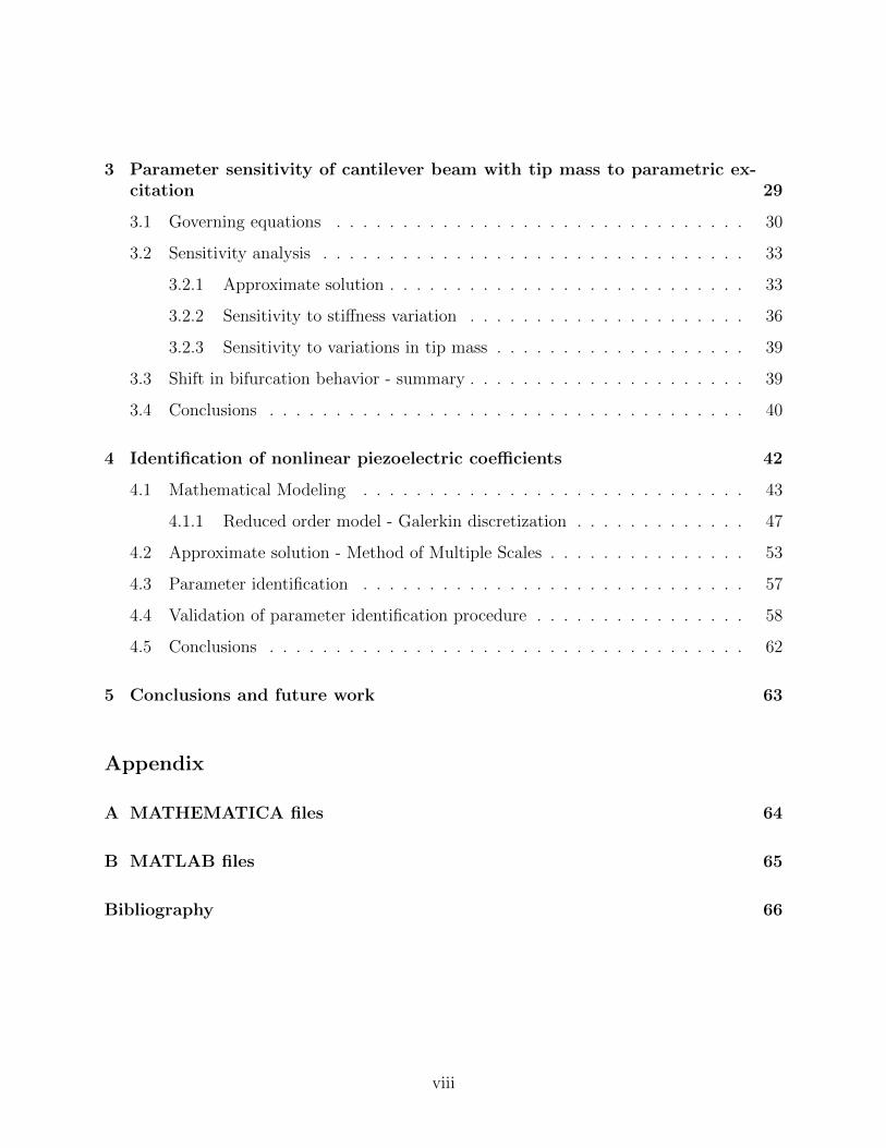
3 Parameter sensitivity of cantilever beam with tip mass to parametric ex-citation 29
3.1 Governing equations . . . . . . . . . . . . . . . . . . . . . . . . . . . . . . . 30
3.2 Sensitivity analysis . . . . . . . . . . . . . . . . . . . . . . . . . . . . . . . . 33
3.2.1 Approximate solution . . . . . . . . . . . . . . . . . . . . . . . . . . . 33
3.2.2 Sensitivity to stiffness variation . . . . . . . . . . . . . . . . . . . . . 36
3.2.3 Sensitivity to variations in tip mass . . . . . . . . . . . . . . . . . . . 39
3.3 Shift in bifurcation behavior - summary . . . . . . . . . . . . . . . . . . . . . 39
3.4 Conclusions . . . . . . . . . . . . . . . . . . . . . . . . . . . . . . . . . . . . 40
4 Identification of nonlinear piezoelectric coefficients 42
4.1 Mathematical Modeling . . . . . . . . . . . . . . . . . . . . . . . . . . . . . 43
4.1.1 Reduced order model - Galerkin discretization . . . . . . . . . . . . . 47
4.2 Approximate solution - Method of Multiple Scales . . . . . . . . . . . . . . . 53
4.3 Parameter identification . . . . . . . . . . . . . . . . . . . . . . . . . . . . . 57
4.4 Validation of parameter identification procedure . . . . . . . . . . . . . . . . 58
4.5 Conclusions . . . . . . . . . . . . . . . . . . . . . . . . . . . . . . . . . . . . 62
5 Conclusions and future work 63
Appendix
A MATHEMATICA files 64
B MATLAB files 65
Bibliography 66
viii
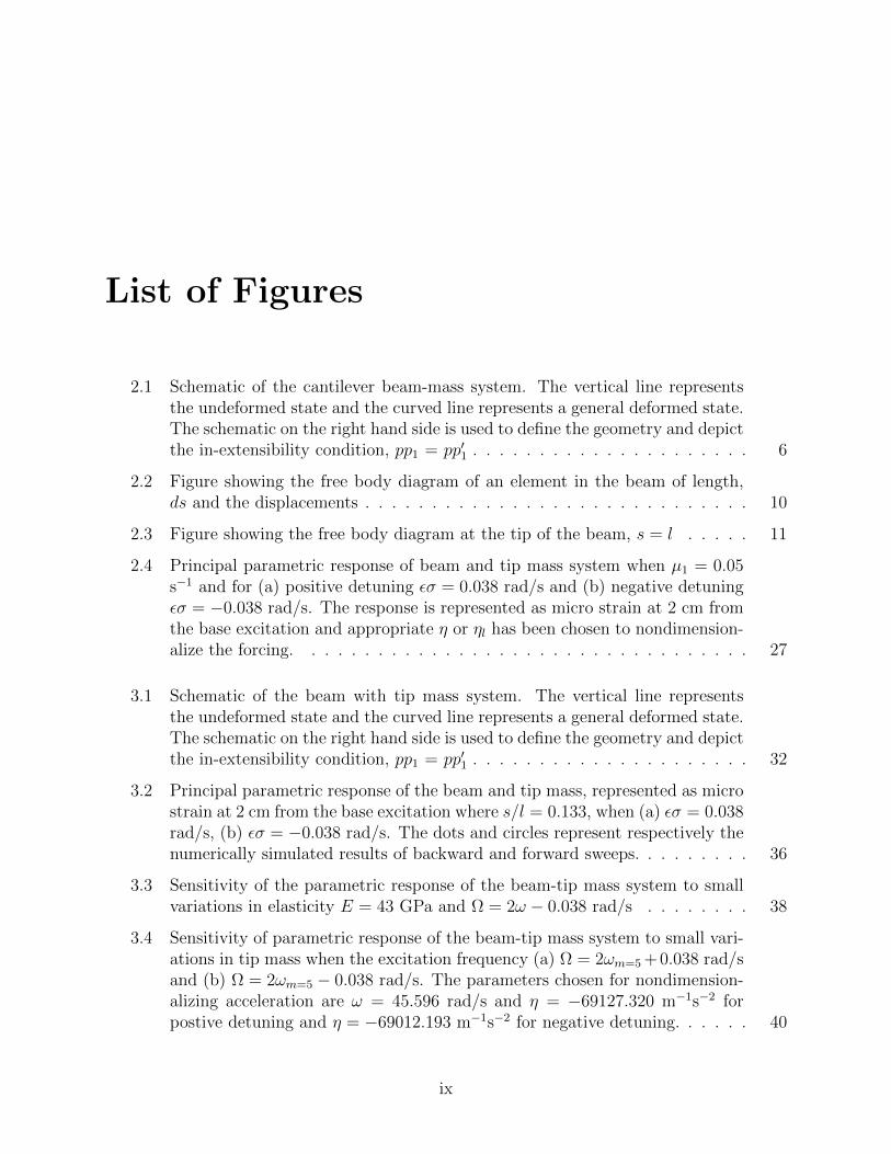
List of Figures
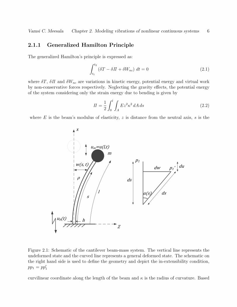
2.1 Schematic of the cantilever beam-mass system. The vertical line representsthe undeformed state and the curved line represents a general deformed state.The schematic on the right hand side is used to define the geometry and depictthe in-extensibility condition, pp1 = pp′1 . . . . . . . . . . . . . . . . . . . . . 6
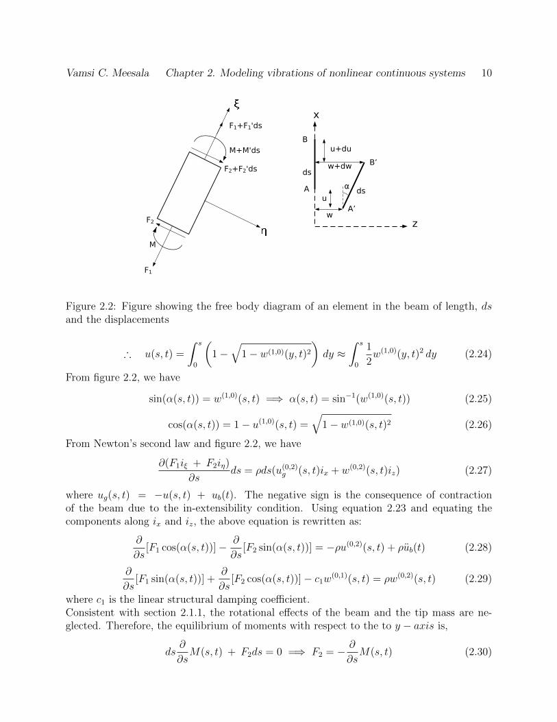
2.2 Figure showing the free body diagram of an element in the beam of length,ds and the displacements . . . . . . . . . . . . . . . . . . . . . . . . . . . . . 10
2.3 Figure showing the free body diagram at the tip of the beam, s = l . . . . . 11
2.4 Principal parametric response of beam and tip mass system when µ1 = 0.05s−1 and for (a) positive detuning εσ = 0.038 rad/s and (b) negative detuningεσ = −0.038 rad/s. The response is represented as micro strain at 2 cm fromthe base excitation and appropriate η or ηl has been chosen to nondimension-alize the forcing. . . . . . . . . . . . . . . . . . . . . . . . . . . . . . . . . . 27
3.1 Schematic of the beam with tip mass system. The vertical line representsthe undeformed state and the curved line represents a general deformed state.The schematic on the right hand side is used to define the geometry and depictthe in-extensibility condition, pp1 = pp′1 . . . . . . . . . . . . . . . . . . . . . 32
3.2 Principal parametric response of the beam and tip mass, represented as microstrain at 2 cm from the base excitation where s/l = 0.133, when (a) εσ = 0.038rad/s, (b) εσ = −0.038 rad/s. The dots and circles represent respectively thenumerically simulated results of backward and forward sweeps. . . . . . . . . 36
3.3 Sensitivity of the parametric response of the beam-tip mass system to smallvariations in elasticity E = 43 GPa and Ω = 2ω − 0.038 rad/s . . . . . . . . 38
3.4 Sensitivity of parametric response of the beam-tip mass system to small vari-ations in tip mass when the excitation frequency (a) Ω = 2ωm=5 + 0.038 rad/sand (b) Ω = 2ωm=5 − 0.038 rad/s. The parameters chosen for nondimension-alizing acceleration are ω = 45.596 rad/s and η = −69127.320 m−1s−2 forpostive detuning and η = −69012.193 m−1s−2 for negative detuning. . . . . . 40
ix
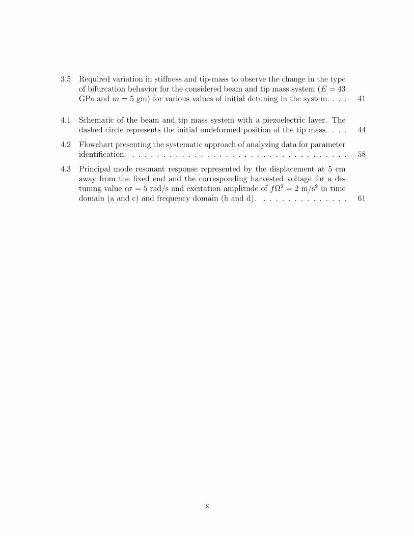
3.5 Required variation in stiffness and tip-mass to observe the change in the typeof bifurcation behavior for the considered beam and tip mass system (E = 43GPa and m = 5 gm) for various values of initial detuning in the system. . . . 41
4.1 Schematic of the beam and tip mass system with a piezoelectric layer. Thedashed circle represents the initial undeformed position of the tip mass. . . . 44
4.2 Flowchart presenting the systematic approach of analyzing data for parameteridentification. . . . . . . . . . . . . . . . . . . . . . . . . . . . . . . . . . . . 58
4.3 Principal mode resonant response represented by the displacement at 5 cmaway from the fixed end and the corresponding harvested voltage for a de-tuning value εσ = 5 rad/s and excitation amplitude of fΩ2 = 2 m/s2 in timedomain (a and c) and frequency domain (b and d). . . . . . . . . . . . . . . 61
x
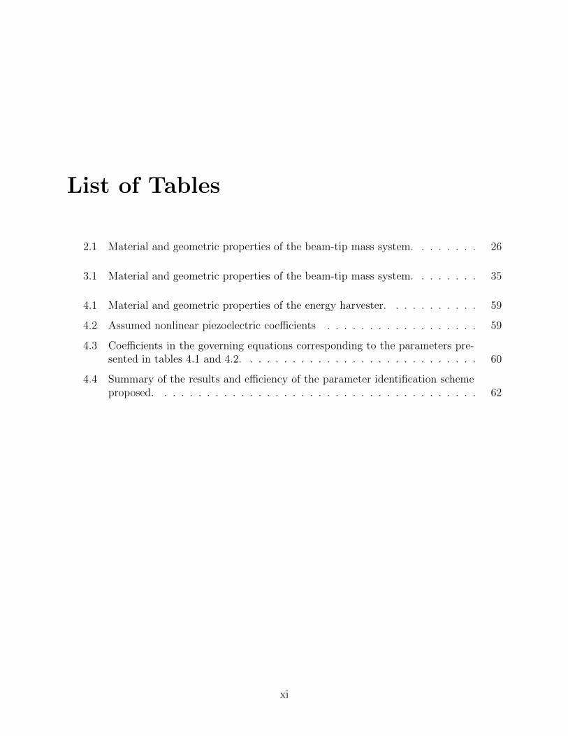
List of Tables
2.1 Material and geometric properties of the beam-tip mass system. . . . . . . . 26
3.1 Material and geometric properties of the beam-tip mass system. . . . . . . . 35
4.1 Material and geometric properties of the energy harvester. . . . . . . . . . . 59
4.2 Assumed nonlinear piezoelectric coefficients . . . . . . . . . . . . . . . . . . 59
4.3 Coefficients in the governing equations corresponding to the parameters pre-sented in tables 4.1 and 4.2. . . . . . . . . . . . . . . . . . . . . . . . . . . . 60
4.4 Summary of the results and efficiency of the parameter identification schemeproposed. . . . . . . . . . . . . . . . . . . . . . . . . . . . . . . . . . . . . . 62
xi

Chapter 1
Introduction
1.1 Motivation
To emphasize the importance of modeling and simulation of dynamical systems, I would liketo start with the definition of Model by Professor Marvin Minsky:
“A model (M) for a system (S) and an experiment (E) is anything to which E can be appliedin order to answer the questions about (S).”
Abiding by the above definition, understanding a physical system is a process that involvesperforming experiments to provide an insight into the principles governing the system andtheir respective models. Although scientists are interested in understanding the system byobserving and developing a model for it, engineers are focused on applying and modifyingthem it to their advantage [1]. Particularly, insights from models and experiments play animportant role in the prognosis of design, as they allow the designer to develop a mathemat-ical model and simulate it. With the computational capabilities of the current digital age,these simulations can provide a quick way to predict a behavior and control it accordingly,which otherwise is done by performing time-consuming and arduous experiments.
Depending on the nature of the response, any mathematical model of a mechanical system(equation/s of motion) can be classified into linear or nonlinear dynamical system. In mostcases, a complete mathematical description of the dynamical system is inherently nonlinear,which under specified conditions may be reduced to a linear description. Some of the stan-dard examples of mechanical systems exhibiting nonlinear response or nonlinear dynamicscan be found in [2–5]. In structures, the nonlinearities in the equation/s of motion ariseeither due to large deformations (geometric nonlinearity), or due to the inertia of motion(inertial nonlinearity) or due to the nonlinear constitutive relation between stress and strain(material nonlinearity) or all of them together. A typical free and un-damped equationof motion of a system including the inertial and geometric nonlinearities until third order
1
Vamsi C. Meesala Chapter 1. Introduction 2
approximation is of the form:
¨q(t) + ω2q(t) + δ[q(t)q(t)2 + q(t)2q(t)
]+ αq(t)3 = 0
In this work, the nonlinear dynamics of a cantilever beam with tip mass are modeled andexploited for interesting objectives as will be discussed in the following paragraphs.
1.2 Background - cantilever beam and tip mass
system
The cantilever beam with a tip mass is a generic system to study and assess different as-pects of structural dynamics. It is utilized to model robotic arms [6,7], antenna masts [8,9],wings with store configurations [10–15], energy harvesting devices [16–22], vibrating beamgyroscopes [23, 24] and bio/chemical sensors [25–31]. In all these applications, there is aneed to validate the mathematical model developed with experimental results to facilitatethe analysis and optimize the design for better performance. Moreover, most of the applica-tions mentioned above utilize the dynamic resonant response or are implicitly nonlinear, thatproduce large strains and induce geometric nonlinearity. This calls for accurate modelingby considering the inherently present geometric nonlinearity up to an appropriate approx-imation. Also, the dynamic resonant response is highly dependent on the geometric andmaterial properties of the device. Any uncertainty in the beam’s stiffness, the mass valueor material properties associated with operational conditions such as environmental thermaleffects, and fatigue induced by cyclic loading or manufacturing tolerances (or defects) canresult in discrepancies between the proposed cantilever beam-mass model and predicted val-ues and experimental results; thereby compromising the fidelity of the model representingthe device. Such discrepancies can be anticipated by performing a sensitivity analysis ofthe response to small variations in the parameters, which will strengthen the model. Theinformation of sensitivity can be precious as it can be used to detect damage or to sense atarget mass using bio/mass sensors.
The problem of nonlinearity in the case of the cantilever beam with tip mass energy harvestersis even more complicated. This is because the piezoelectric material commonly employedfor energy harvesting applications [17], can behave in a nonlinear manner by exhibitingamplitude dependent resonant frequency, super-harmonics in the response, saturation andhysteresis behaviors [32–34]. It is important to understand the nature of the nonlinearity byestimating the nonlinear parameters in the constitutive relations. An optimized curve fittingprocedure can be used to identify the parameters causing the nonlinear behavior. Yet, thereis a need for more parameter identification procedures that exploit the vibration response.We cater to all ideas and issues mentioned above in this work with the following objectives.
Vamsi C. Meesala Chapter 1. Introduction 3
1.3 Objectives
The primary objectives of this work are:
• To accurately develop the governing equation of a cantilever beam tip-mass systemsubjected to parametric excitation with particular consideration of nonlinear boundaryconditions and their effects on governing equation.
• To perform sensitivity of the parametric response of the cantilever beam tip-mass sys-tem to small variations for design purposes or for exploring specific response dynamicsto detect variations.
• To propose a parameter identification scheme based on direct excitation of a cantileverbeam tip-mass system to identify and quantify the nonlinear piezoelectric coefficientsin constitutive relations.
We solve all the above-mentioned objectives using the framework of the method of multiplescales.
Chapter 2
Response variations of a cantileverbeam tip mass system with nonlinearand linearized boundary conditions
A crucial step in the design of any structure is to understand its dynamic response. This typ-ically includes determining its natural frequencies, corresponding mode shapes, and dynamicstresses. Such an exercise can be performed by reduced order mathematical models that pre-dict this response. The cantilever beam with a tip mass has been used as a generic system toassess modeling needs in different applications or as a structural system whose response canbe exploited for different purposes. For example, treating the boundary conditions at thefree end of the cantilever beam tip mass system can shed light on how to treat wing/storeconfigurations in flutter analysis of fighter aircraft [10–14]. In energy harvesting of ambientvibrations, the tip mass is added to cantilevered piezoelectric layered beam structure to in-duce large strains thereby generating high power density [16,17]. In microelectro mechanicalsystems, adding a tip mass decreases the natural frequency, which otherwise would be of theorder of few GHz’s [18–22]. In gas/mass sensors, the response of the cantilever beam in con-junction with added target mass can be used to sense the presence of bio-materials [25–31].It is also modeled to understand coupling and energy transfer phenomenon in structures forcontrol purposes [35–37].
The governing equations and boundary conditions of continuous systems, which are usuallyintegro-partial differential equations, can be solved numerically using the Finite ElementMethods [38]. Alternatively, a reduced-order model or representation of the system’s dy-namics can be treated analytically by using perturbation methods. The advantages of thesemethods is their flexibility to investigate stability and characteristics of nonlinear response.Direct [39–43] and Discretization [41,44,45] approaches can be used when implementing thesemethods. In the direct approach, the method of multiple scales is directly applied to thegoverning partial differential equation. By isolating the secular terms and using the adjoint
4
Vamsi C. Meesala Chapter 2. Modeling vibrations of nonlinear continuous systems 5
description, solvability conditions are developed from which amplitude and phase modula-tion equations that govern the system’s response are obtained [46]. In the discretizationapproach, a Galerkin weighted residual method is used to develop the governing equation ofn modes from the distributed system given by the partial differential equation and boundaryconditions. Then, the governing equations are solved using the method of multiple scalesto develop amplitude and phase modulation equations by eliminating the secular terms [41].That is, for an excitation near a particular mode, the problem of solving a PDE and boundaryconditions in the direct approach is reduced to one or more ODE in discretized approach.
It is usually assumed that linearizing the boundary conditions is justified especially whenthe interest is in finding linear mode shapes and natural frequency of system. On the otherhand, it is fair to expect that the nature of the response of a nonlinear system may varysignificantly from the true one if the boundary conditions were linearized. This chapterexamines the extent of such variations in the response of a cantilever beam with tip masssystem. Furthermore, particular attention is paid to the effect of linearization on the dis-cretized governing equations and their solution. Towards this objective, we develop thedistributed parameter governing equations and boundary conditions for a parametrically ex-cited cantilever beam and tip mass system using the generalized Hamilton’s principle [47].We then employ Galerkin discretization to the distributed model and determine the gov-erning equation of the first mode (discretized equation) to study the principal parametricresonance by considering and neglecting nonlinear boundary conditions. Thereafter, we solvethe distributed parameter system and discretized equation with nonlinear boundary condi-tions using the method of multiple scales and compare the resulting modulation equationswith those obtained from the PDE solution to validate the discretization.
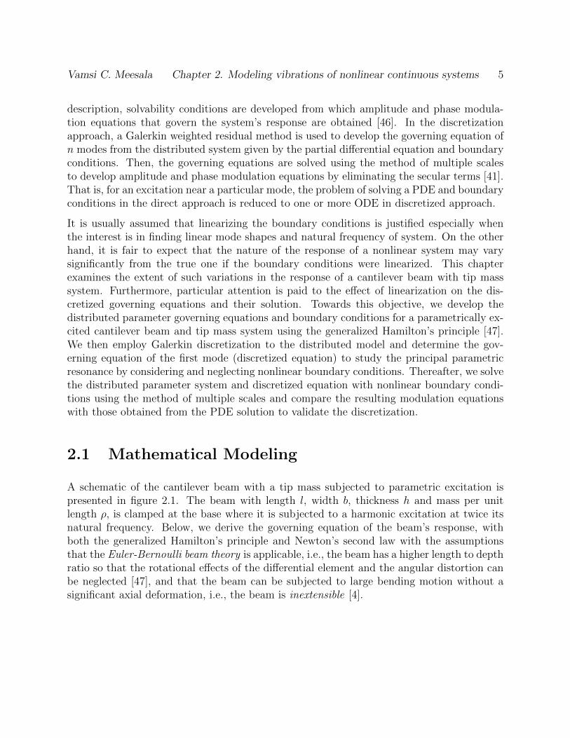
2.1 Mathematical Modeling
A schematic of the cantilever beam with a tip mass subjected to parametric excitation ispresented in figure 2.1. The beam with length l, width b, thickness h and mass per unitlength ρ, is clamped at the base where it is subjected to a harmonic excitation at twice itsnatural frequency. Below, we derive the governing equation of the beam’s response, withboth the generalized Hamilton’s principle and Newton’s second law with the assumptionsthat the Euler-Bernoulli beam theory is applicable, i.e., the beam has a higher length to depthratio so that the rotational effects of the differential element and the angular distortion canbe neglected [47], and that the beam can be subjected to large bending motion without asignificant axial deformation, i.e., the beam is inextensible [4].
Vamsi C. Meesala Chapter 2. Modeling vibrations of nonlinear continuous systems 6
2.1.1 Generalized Hamilton Principle
The generalized Hamilton’s principle is expressed as:∫ t2
t1
(δT − δΠ + δWnc) dt = 0 (2.1)
where δT , δΠ and δWnc are variations in kinetic energy, potential energy and virtual workby non-conservative forces respectively. Neglecting the gravity effects, the potential energyof the system considering only the strain energy due to bending is given by
Π =1
2
∫ l
0
∫A
Ez2κ2 dAds (2.2)
where E is the beam’s modulus of elasticity, z is distance from the neutral axis, s is the
Z
x
ub(t)
sl
w(s, t)
um=u(l,t)
p1
p1'dw
ds
ds
du
α(s)
ρ
m
h
Figure 2.1: Schematic of the cantilever beam-mass system. The vertical line represents theundeformed state and the curved line represents a general deformed state. The schematic onthe right hand side is used to define the geometry and depict the in-extensibility condition,pp1 = pp′1
curvilinear coordinate along the length of the beam and κ is the radius of curvature. Based
Vamsi C. Meesala Chapter 2. Modeling vibrations of nonlinear continuous systems 7
on the assumption that the beam is in extensible, the curvature is expressed as
κ =∂
∂sα(s, t) = w(2,0)(s, t) +
1
2w(2,0)(s, t)w(1,0)(s, t)2 + ... (2.3)
where the notation (.)(n1,n2)(s, t) denotes nth1 derivative of (.) with respect to s and nth2derivative of (.) with respect to t. This notation is followed quite extensively from here on.Squaring equation 2.3 yields
κ2 =[w(2,0)(s, t)
]2+[w(2,0)(s, t)w(1,0)(s, t)
]2+ ... (2.4)
Dropping all terms that give rise to nonlinearities with order larger than three, i.e., O ([.]n>3) =0, the potential energy, Π is re-written as
Π =1
2
∫ l
0
∫A
Ez2([w(2,0)(s, t)
]2+[w(2,0)(s, t)w(1,0)(s, t)
]2)dAds (2.5)
and noting that the area moment of inertia about the Y-axis is given by IY =∫Az2 dA, we
write the potential energy as
Π =1
2
∫ l
0
EIY[w(2,0)(s, t)
]2ds+
1
2
∫ l
0
EIY[w(1,0)(s, t)w(2,0)(s, t)
]2ds (2.6)
The kinetic energy of the beam-tip mass system is given by
T =1
2m
([um(t)]2 +
[∂w(l, t)
∂t
]2)
+1
2
∫ l
0
ρ
([u(0,1)(s, t)
]2+
[∂w(s, t)
∂t
]2)ds (2.7)
where u(s, t) and um(t) represent respectively the vertical displacements of the beam and tipmass. The relations between these displacements is determined from the geometry of figure2.1. We write
α(s, t) = sin−1(w(1,0)(s, t)
), and (2.8)
cos(α(s, t)) =∂s− ∂u(s, t)
∂s= 1− u(1,0)(s, t) (2.9)
Expanding the inverse trigonometric and trigonometric functions, we re-write equations 2.8-2.9 as
α(s, t) = w(1,0)(s, t) +1
6
[w(1,0)(s, t)
]3+ ... , and (2.10)
u(1,0)(s, t) =1
2[α(s, t)]2 − 1
24[α(s, t)]4 − ... (2.11)
Substituting equation 2.10 into equation 2.11, we obtain
u(1,0)(s, t) =1
2
[w(1,0)(s, t)
]2+O
([w(1,0)(s, t)
]5)(2.12)

Vamsi C. Meesala Chapter 2. Modeling vibrations of nonlinear continuous systems 8
where O([w(1,0)(s, t)
]5)is used to represent higher order terms that are neglected in the
subsequent analysis. Representing the harmonic excitation of the base by ub, the verticaldisplacement of the tip mass is then given by
um(t) =
∫ l
0
1
2
[w(1,0)(s, t)
]2ds− ub(t) (2.13)
Similarly, the vertical displacement of any element on the beam at a distance s from thebase is given by
u(s, t) =
∫ s
0
1
2
[w(1,0)(y, t)
]2dy − ub(t) (2.14)
Substituting the values of um and us from equations 2.13 and 2.14 into equation 2.7, weobtain
T =1
2m
[∫ l
0
1
2
∂
∂t
(∂w(s, t)
∂s
)2
ds− ub(t)
]2
+1
2
∫ l
0
ρ
[∫ s
0
1
2
∂
∂t
(∂w(y, t)
∂y
)2
dy − ub(t)
]2
ds
+1
2m
(∂w(l, t)
∂t
)2
+1
2
∫ l
0
ρ
(∂w(s, t)
∂t
)2
ds (2.15)
It has been assumed that the tip mass is treated as a point mass and, hence, the rotationaleffects are not included when determining the kinetic energy.
The virtual work done by the non conservative forces is given by
δWnc = −∫ l
0
c1w(0,1)(s, t)δw(s, t) ds (2.16)
where, c1 is structural damping coefficient.
Substituting equations 2.6, 2.15 and 2.16 into equation 2.1, we obtain the equation of motionas
− ρw − c1w −ρw′
2
∫ s
0
∂2
∂t2(w′2)dy + ρubw
′ − EIY (w′′′′ + w′′3 + 4w′w′′w′′′ + w′2w′′′′)
+ w′′(ρ
2
∫ l
s
∫ θ
0
∂2
∂t2(w′2)dy dθ +m
∫ l
0
∂2
∂t2
(w′2
2
)ds−mub − (l − s)ρub
)= 0 (2.17)
In deriving equation 2.17, we used the integration by parts as∫ l
0
∫ s0G(y) dy ds =
∫ l0(l −
s)G(s) ds, where G(x) is any continuous function.
Using (w′(w′w′′)′)′ = w′′3+4w′w′′w′′′+w′2w′′′′ and ρ2
(w′∫ sl
∫ θ0
∂2
∂t2(w′2) dy dθ
)′=ρw′
2
∫ s0
∂2
∂t2(w′2) dy
+ w′′ρ
2
∫ ls
∫ θ0
∂2
∂t2(w′2) dy dθ, equation 2.17 is further simplified to obtain
Vamsi C. Meesala Chapter 2. Modeling vibrations of nonlinear continuous systems 9
ρw + c1w + EIY (w′′′′ + [w′(w′w′′)′]′) +mubw′′ +
ρ
2
(w′∫ s
l
∫ θ
0
∂2
∂t2(w′2)dy dθ
)′− ρub (w′ + (s− l)w′′)− mw′′
2
∫ l
0
∂2
∂t2(w′2)ds = 0 (2.18)
where ub = −12fΩ2
[ej(ΩT0+τe) + e−j(ΩT0+τe)
]and f is displacement of the excitation and Ω is
the forcing frequency. The natural nonlinear boundary conditions at s = l are determinedfrom the moment and the shear boundary conditions as(
EIYw′′w′2 + EIYw
′′) |s=l = 0 =⇒ w(2,0)(l, t) = 0 (2.19)(mubw
′ −mw′∫ l
0
∂2
∂t2
(w′2
2
)ds+ EIY
(w′′′w′2 + w′′2w′ + w′′′
)−mw
)∣∣∣∣s=l
= 0 (2.20)
Since the beam is clamped, the geometric boundary conditions at s = 0 are given by
w(0, t) = 0 (2.21)
∂w(s, t)
∂s
∣∣∣∣s=0
= 0 (2.22)
We shall note that in the above derivation, E, IY , l, ρ and m are assumed to be constants,that y and θ are dummy variables, and that the primes and dots represent derivatives ofw(s, t) with respect to the coordinate s and time t respectively. The MATHEMATICA codeGenhamilton1.0.nb, used for the complete derivation can be found in Appendix A.
2.1.2 Newton’s Second Law
The procedure of Nayfeh and Pai [4] is followed below to derive the fully nonlinear governingequations of initially straight Euler-Bernoulli beams. A local orthogonal co-ordinate systemξyη is considered for a better representation of the forces. The free body diagram of anelement of beam of length ds is shown in the figure 2.2 where F1 and F2 are surface tractionforces along the ξ and η directions respectively. If ix and iz are unit vectors along x andz axes and iξ and iη are unit vectors along the ξ and η axes, there exists a transformationmatrix T , such that,
ixiz
= [T ]
iξiη
, [T ] =
[cosα sinα− sinα cosα
](2.23)
By considering u(s, t) and w(s, t) as the displacements along the x and z axes respectivelyand using the in-extensibility condition, we write,[
1− u(1,0)(s, t)]2
+ w(1,0)(s, t)2 = 1
Vamsi C. Meesala Chapter 2. Modeling vibrations of nonlinear continuous systems 10
F1
F1+F1'ds
F2
F2+F2'ds
M
M+M'ds
x
z
A
B
B’
A’
u
w
w+dw
u+du
α
ds
ds
Figure 2.2: Figure showing the free body diagram of an element in the beam of length, dsand the displacements
∴ u(s, t) =
∫ s
0
(1−
√1− w(1,0)(y, t)2
)dy ≈
∫ s
0
1
2w(1,0)(y, t)2 dy (2.24)
From figure 2.2, we have
sin(α(s, t)) = w(1,0)(s, t) =⇒ α(s, t) = sin−1(w(1,0)(s, t)) (2.25)
cos(α(s, t)) = 1− u(1,0)(s, t) =√
1− w(1,0)(s, t)2 (2.26)
From Newton’s second law and figure 2.2, we have
∂(F1iξ + F2iη)
∂sds = ρds(u(0,2)
g (s, t)ix + w(0,2)(s, t)iz) (2.27)
where ug(s, t) = −u(s, t) + ub(t). The negative sign is the consequence of contractionof the beam due to the in-extensibility condition. Using equation 2.23 and equating thecomponents along ix and iz, the above equation is rewritten as:
∂
∂s[F1 cos(α(s, t))]− ∂
∂s[F2 sin(α(s, t))] = −ρu(0,2)(s, t) + ρub(t) (2.28)
∂
∂s[F1 sin(α(s, t))] +
∂
∂s[F2 cos(α(s, t))]− c1w
(0,1)(s, t) = ρw(0,2)(s, t) (2.29)
where c1 is the linear structural damping coefficient.Consistent with section 2.1.1, the rotational effects of the beam and the tip mass are ne-glected. Therefore, the equilibrium of moments with respect to the to y − axis is,
ds∂
∂sM(s, t) + F2ds = 0 =⇒ F2 = − ∂
∂sM(s, t) (2.30)
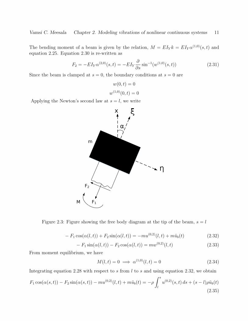
Vamsi C. Meesala Chapter 2. Modeling vibrations of nonlinear continuous systems 11
The bending moment of a beam is given by the relation, M = EIY k = EIY α(1,0)(s, t) and
equation 2.25. Equation 2.30 is re-written as
F2 = −EIY α(2,0)(s, t) = −EIY∂
∂ssin−1(w(1,0)(s, t)) (2.31)
Since the beam is clamped at s = 0, the boundary conditions at s = 0 are
w(0, t) = 0
w(1,0)(0, t) = 0
Applying the Newton’s second law at s = l, we write
F1
F2
M
m
x
α
Figure 2.3: Figure showing the free body diagram at the tip of the beam, s = l
− F1 cos(α(l, t)) + F2 sin(α(l, t)) = −mu(0,2)(l, t) +mub(t) (2.32)
− F1 sin(α(l, t))− F2 cos(α(l, t)) = mw(0,2)(l, t) (2.33)
From moment equilibrium, we have
M(l, t) = 0 =⇒ α(1,0)(l, t) = 0 (2.34)
Integrating equation 2.28 with respect to s from l to s and using equation 2.32, we obtain
F1 cos(α(s, t))− F2 sin(α(s, t))−mu(0,2)(l, t) +mub(t) = −ρ∫ s
l
u(0,2)(s, t) ds+ (s− l)ρub(t)
(2.35)
Vamsi C. Meesala Chapter 2. Modeling vibrations of nonlinear continuous systems 12
From equations 2.24 and 2.35, the expression for F1 is obtained as
F1 =1
cos(α(s, t))
[−ρ
2
∫ s
l
∫ θ
0
∂2
∂t2(w(1,0)(y, t)2
)dy dθ + (s− l)ρub(t)
]+
1
cos(α(s, t))
[F2 sin(α(s, t)) +
m
2
∫ l
0
∂2
∂t2(w(1,0)(s, t)2
)ds−mub(t)
](2.36)
Substituting the expression for F1 in equation 2.29 and using the trigonometric relations inequations 2.25 and 2.26, we obtain
− ρ
2
∂
∂s
(w(1,0)(s, t)√
1− w(1,0)(s, t)2
∫ s
l
∫ θ
0
∂2
∂t2(w(1,0)(y, t)2
)dy dθ
)− c1w
(0,1)(s, t)
− c2w(0,1)(s, t)|w(0,1)(s, t)|+ ∂
∂s
(ρub(t)(s− l)w(1,0)(s, t)√
1− w(1,0)(s, t)2
)+
∂
∂s
(F2√
1− w(1,0)(s, t)2
)
+∂
∂s
(w(1,0)(s, t)√
1− w(1,0)(s, t)2
[m
2
∫ l
0
∂2
∂t2(w(1,0)(s, t)2
)ds−mub(t)
])= ρw(0,2)(s, t) (2.37)
Substituting the expression for F2 from equation 2.31, using Taylor series expansion of inversetrigonometric functions and retaining the expression up to the third order, we obtain
ρw + c1w + c2|w|w + EIY (w′′′′ + (w′(w′w′′)′)′) +mubw′′ +
ρ
2
(w′∫ s
l
∫ θ
0
∂2
∂t2(w′2)dy dθ
)′− ρub(t) (w′ + (s− l)w′′)− mw′′
2
∫ l
0
∂2
∂t2(w′′2)ds = 0 (2.38)
Substituting the expressions for F1, F2, cos(α(s, t)), α(1,0)(s, t) and sin(α(s, t)) into theboundary conditions at s = l i.e., equations 2.33 and 2.34, we obtain the modified boundaryconditions as
w′′(l, t) = 0 (2.39)(mubw
′ −mw′∫ l
0
∂2
∂t2
(w′2
2
)ds+ EIY
(w′′′w′2 + w′′2w′ + w′′′
)−mw
)∣∣∣∣s=l
= 0 (2.40)
The dashes and dots represent derivatives of w(s, t) with respect to s and time, t respectively,and y and θ are dummy variables.We observe that equations 2.18 - 2.20 and 2.38 - 2.40, representing governing equation andboundary conditions derived using Newton’s second law exactly agree with those derivedusing the generalized Hamilton’s principle.
Vamsi C. Meesala Chapter 2. Modeling vibrations of nonlinear continuous systems 13
2.2 Reduced order model - Galerkin discretization
Next, we perform modal analysis by solving for the exact mode shapes and orthogonalequations. Then, we use the Galerkin discretization procedure to derive and note the differ-ences in the governing equation of the first mode when considering linearized and nonlinearboundary conditions.
2.2.1 Modal analysis
Modal analysis, used to determine the mode shapes and frequencies of the beam-mass sys-tem, is performed by considering the linear undamped free vibration problem obtained bydropping the damping, forcing and nonlinear terms in equations 2.18-2.22, which reducesthe equation of motion to
ρw + EIYw′′′′ = 0 (2.41)
and the boundary conditions tow(0, t) = 0 (2.42)
∂w(s, t)
∂s
∣∣∣∣s=0
= 0 (2.43)(EIYw
′′w′2 + EIYw′′) |s=l = 0 =⇒ w′′|s=l = 0 (2.44)
(EIYw′′′ −mw) |s=l = 0 (2.45)
Considering equation 2.41, we observe that the spatial and temporal derivatives of w(x, t)can be explicitly decomposed into two degenerate equations. So, w(x, t) is decomposed intoa product of independent spatial and temporal functions and written as
w(s, t) = φ(s)q(t) (2.46)
Substituting equation 2.46 into equation 2.41 and realizing that q = −ω2nq, where ωn is the
natural frequency of the nth-mode, we obtain,
φ′′′′ = λ4φ (2.47)
whose general solution is of the form
φ(s) = A cos(λs) +B sin(λs) + C cosh(λs) +D sinh(λs) (2.48)
where λ =(ω2nρ
EIY
) 14
and the linear boundary conditions are given by
φ(0) = φ′(0) = φ′′(l) = 0 (2.49)(EIY φ
′′′ +mω2φ)|s=l = 0 (2.50)

Vamsi C. Meesala Chapter 2. Modeling vibrations of nonlinear continuous systems 14
Substituting the general solution in the linear boundary conditions and solving for non-trivialsolution yields the characteristic equation as:
ρ [cos (λl) cosh (λl) + 1] +mλ [cos (λl) sinh (λl)− sin (λl) cosh (λl)] = 0 (2.51)
The characteristic equation is a transcendental equation. It has infinite solutions for λ (andω) and, hence, an infinite number of modes. For any two distinct modes, p and q, equation2.47 follows the orthogonality conditions [47]:∫ l
0
ρφp(s)φq(s) ds+mφp(l)φq(l) = δpq∫ l
0
EIY φ′′p(s)φ
′′q(s) ds = δpqω
2q
(2.52)
where δpq is the Kronecker delta, defined as unity when p is equal to q and zero otherwise.Using the above discretization, the solution is then approximated by the sum of a finitenumber of modes, i.e.
w(s, t) =M∑i=1
φi(s)qi(t) (2.53)
where the basis function φi(s) represents the mode shape, qi(t) represents the modal coordi-nate, and M is the number of modes under consideration. We note that the basis functionis a comparable function as it satisfies the linear boundary conditions.
2.2.2 Third order non-linear equation of motion
To develop the third order non-linear equation of motion of modal coordinates, which fromnow, will be referred as temporal amplitudes, we substitute w(s, t) =
∑Mi=1 φi(s)qi(t) for
w(s, t) into equation 2.18, which yields
ρM∑i=1
qiφi + c1
M∑i=1
qiφi + EIY
[M∑i=1
φ′′′′i qi +M∑
i,j,k=1
qiqjqk(φ′i(φ′jφ′′k)′)′
]+mub
M∑i=1
φ′′i qi
+ρ
2
M∑i,j,k=1
(φ′iqi
∫ s
l
∫ θ
0
φ′jφ′k
d2
dt2(qjqk) dy dθ
)′− ρub
M∑i=1
qi (φ′i + (s− l)φ′′i )
−M∑
i,j,k=1
mφ′′i qi2
∫ l
0
φ′jφ′k
d2
dt2(qjqk) ds = 0 (2.54)
By considering only M modes, the discretization doesn’t fully satisfy equation 2.18 in thatthe right hand side may differ from zero. One could then represent this difference in equa-tion 2.54 by a residue R on its right hand side. We employ Galerkin’s weighted residual
Vamsi C. Meesala Chapter 2. Modeling vibrations of nonlinear continuous systems 15
procedure, for the formulation of the equation/s governing temporal amplitudes qi(t) thatrequire the residue to be orthogonal to the comparison functions φi(s), linear mode shapesor basis functions [48,49]. Therefore, the equation is multiplied with a mode shape φr(s) andintegrated over the length of the beam. This procedure not only accounts for the residue butalso enables us to employ the orthogonality conditions as stated in equation 2.52 to developthe governing equation/s of the temporal amplitudes.
Considering only one mode(M = 1) and using the orthogonal properties of the linear modes,the individual terms in equation 2.54 are simplified as shown below:
q1
∫ l
0
ρφ1φ1 ds = q1 −mq1φ1(l)2
c1q1
∫ l
0
φ21 ds = c1q1
∫ l
0
φ21 ds
EIY q1
∫ l
0
φ1φ′′′′1 dx = ω2
1q1 + EIY q1φ′′′1 (l)φ1(l)
EIY q31
∫ l
0
φ1(φ′1(φ′1φ′′1)′)′ ds = (EIY q
31φ1φ
′21 φ′′′1 )|s=l − EIY q3
1
∫ l
0
φ′21 (φ′1φ′′1)′ ds
mubq1
∫ l
0
φ1φ′′1 ds = mubφ
′1(l)q1φ1(l)−mubq1
∫ l
0
φ′21 ds
ρq1(q21 +q1q1)
∫ l
0
φ1
(φ′1
∫ s
l
∫ θ
0
φ′21 dy dθ
)′ds = −ρq1(q2
1 +q1q1)
∫ l
0
φ′21
(∫ s
l
∫ θ
0
φ′21 dy dθ
)ds
−ρubq1
∫ l
0
φ1(φ′1 + (s− l)φ′′1) ds = −ρubq1
∫ l
0
(l − s)φ′21 ds
−mq1(q1q1+q21)
∫ l
0
φ1φ′′1
(∫ l
0
φ′21 dy
)ds = mq1(q1q1+q2
1)
[−(φ′1φ1
∫ l
0
φ′21 ds)|s=l +
(∫ l
0
φ′21 ds
)2]
The governing equation of first modal co-ordinate, q1, is then written as:
q1 + c1q1
∫ l
0
φ21 ds+ ω2
1q1 − EIY q31
∫ l
0
φ′21 (φ′1φ′′1)′ +mq1(q1q1 + q2
1)
[∫ l
0
φ′21 ds
]2
−mubq1
∫ l
0
φ′21 ds− ρq1(q1q1 + q21)
∫ l
0
φ′21
(∫ s
l
∫ θ
0
φ′21 dy dθ
)ds− ρubq1
∫ l
0
(l − s)φ′21 ds
+φ1
(−mq1φ1 + EIY q1φ
′′′1 (1 + q2
1φ′21 )−mq1(q1q1 + q2
1)
[∫ l
0
φ′21 ds
]φ′1 +mubq1φ
′1
)|s=l = 0
(2.55)
The subscripts representing the mode shape are disregarded in the following sections for thesake of convenience.
Vamsi C. Meesala Chapter 2. Modeling vibrations of nonlinear continuous systems 16
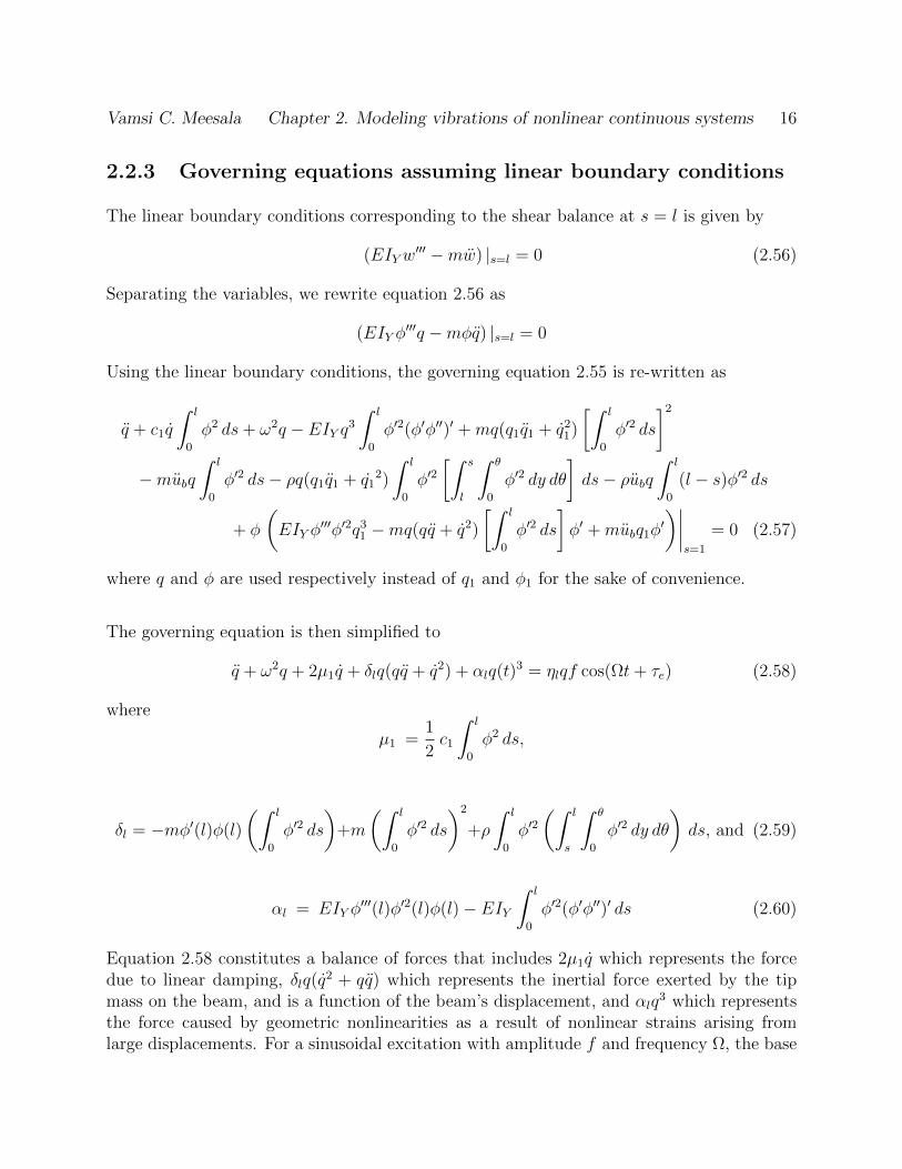
2.2.3 Governing equations assuming linear boundary conditions
The linear boundary conditions corresponding to the shear balance at s = l is given by
(EIYw′′′ −mw) |s=l = 0 (2.56)
Separating the variables, we rewrite equation 2.56 as
(EIY φ′′′q −mφq) |s=l = 0
Using the linear boundary conditions, the governing equation 2.55 is re-written as
q + c1q
∫ l
0
φ2 ds+ ω2q − EIY q3
∫ l
0
φ′2(φ′φ′′)′ +mq(q1q1 + q21)
[∫ l
0
φ′2 ds
]2
−mubq∫ l
0
φ′2 ds− ρq(q1q1 + q12)
∫ l
0
φ′2[∫ s
l
∫ θ
0
φ′2 dy dθ
]ds− ρubq
∫ l
0
(l − s)φ′2 ds
+ φ
(EIY φ
′′′φ′2q31 −mq(qq + q2)
[∫ l
0
φ′2 ds
]φ′ +mubq1φ
′)∣∣∣∣
s=1
= 0 (2.57)
where q and φ are used respectively instead of q1 and φ1 for the sake of convenience.
The governing equation is then simplified to
q + ω2q + 2µ1q + δlq(qq + q2) + αlq(t)3 = ηlqf cos(Ωt+ τe) (2.58)
where
µ1 =1
2c1
∫ l
0
φ2 ds,
δl = −mφ′(l)φ(l)
(∫ l
0
φ′2 ds
)+m
(∫ l
0
φ′2 ds
)2
+ρ
∫ l
0
φ′2(∫ l
s
∫ θ
0
φ′2 dy dθ
)ds, and (2.59)
αl = EIY φ′′′(l)φ′2(l)φ(l)− EIY
∫ l
0
φ′2(φ′φ′′)′ ds (2.60)
Equation 2.58 constitutes a balance of forces that includes 2µ1q which represents the forcedue to linear damping, δlq(q
2 + qq) which represents the inertial force exerted by the tipmass on the beam, and is a function of the beam’s displacement, and αlq
3 which representsthe force caused by geometric nonlinearities as a result of nonlinear strains arising fromlarge displacements. For a sinusoidal excitation with amplitude f and frequency Ω, the base
Vamsi C. Meesala Chapter 2. Modeling vibrations of nonlinear continuous systems 17
acceleration is given by ub = f cos(Ωt+ τe), which yields ub = −fΩ2 cos(Ωt+ τe). As such,we have
ηl = −Ω2
[mφ′(l)φ(l) +m
∫ l
0
φ′2 ds+ ρ
∫ l
0
(l − s)φ′2 ds]
(2.61)
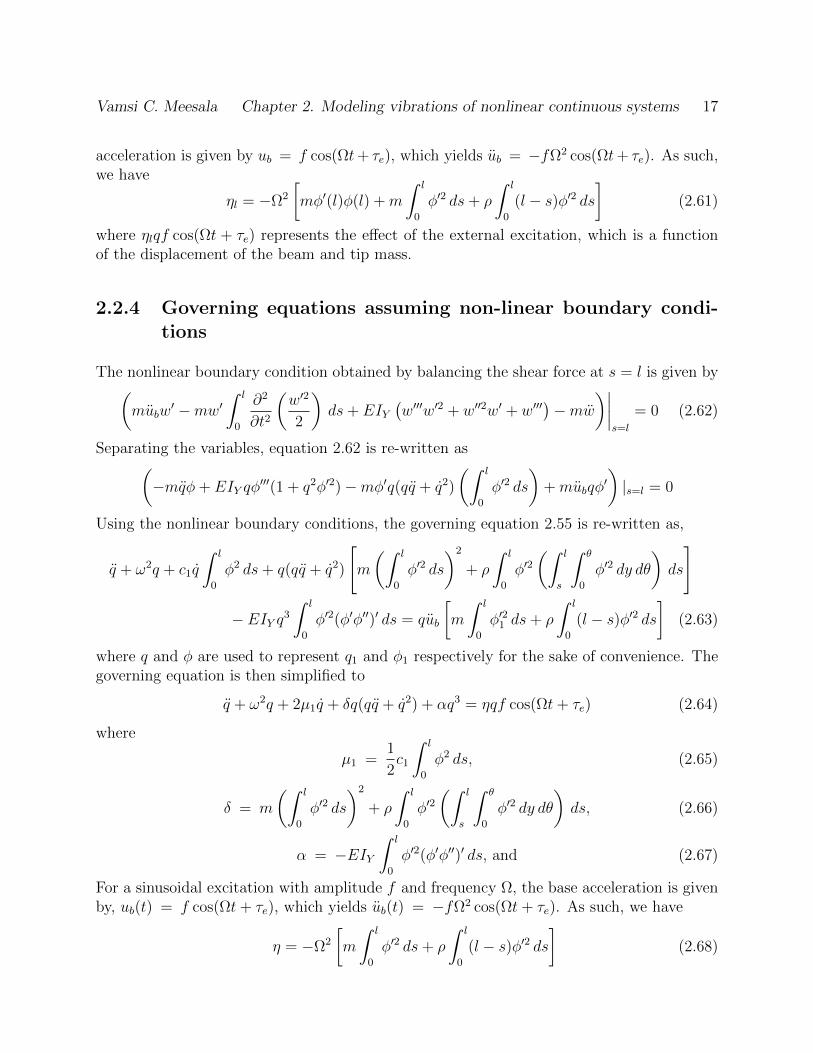
where ηlqf cos(Ωt + τe) represents the effect of the external excitation, which is a functionof the displacement of the beam and tip mass.
2.2.4 Governing equations assuming non-linear boundary condi-tions
The nonlinear boundary condition obtained by balancing the shear force at s = l is given by(mubw
′ −mw′∫ l
0
∂2
∂t2
(w′2
2
)ds+ EIY
(w′′′w′2 + w′′2w′ + w′′′
)−mw
)∣∣∣∣s=l
= 0 (2.62)
Separating the variables, equation 2.62 is re-written as(−mqφ+ EIY qφ
′′′(1 + q2φ′2)−mφ′q(qq + q2)
(∫ l
0
φ′2 ds
)+mubqφ
′)|s=l = 0
Using the nonlinear boundary conditions, the governing equation 2.55 is re-written as,
q + ω2q + c1q
∫ l
0
φ2 ds+ q(qq + q2)
[m
(∫ l
0
φ′2 ds
)2
+ ρ
∫ l
0
φ′2(∫ l
s
∫ θ
0
φ′2 dy dθ
)ds
]
− EIY q3
∫ l
0
φ′2(φ′φ′′)′ ds = qub
[m
∫ l
0
φ′21 ds+ ρ
∫ l
0
(l − s)φ′2 ds]
(2.63)
where q and φ are used to represent q1 and φ1 respectively for the sake of convenience. Thegoverning equation is then simplified to
q + ω2q + 2µ1q + δq(qq + q2) + αq3 = ηqf cos(Ωt+ τe) (2.64)
where
µ1 =1
2c1
∫ l
0
φ2 ds, (2.65)
δ = m
(∫ l
0
φ′2 ds
)2
+ ρ
∫ l
0
φ′2(∫ l
s
∫ θ
0
φ′2 dy dθ
)ds, (2.66)
α = −EIY∫ l
0
φ′2(φ′φ′′)′ ds, and (2.67)
For a sinusoidal excitation with amplitude f and frequency Ω, the base acceleration is givenby, ub(t) = f cos(Ωt+ τe), which yields ub(t) = −fΩ2 cos(Ωt+ τe). As such, we have
η = −Ω2
[m
∫ l
0
φ′2 ds+ ρ
∫ l
0
(l − s)φ′2 ds]
(2.68)
Vamsi C. Meesala Chapter 2. Modeling vibrations of nonlinear continuous systems 18
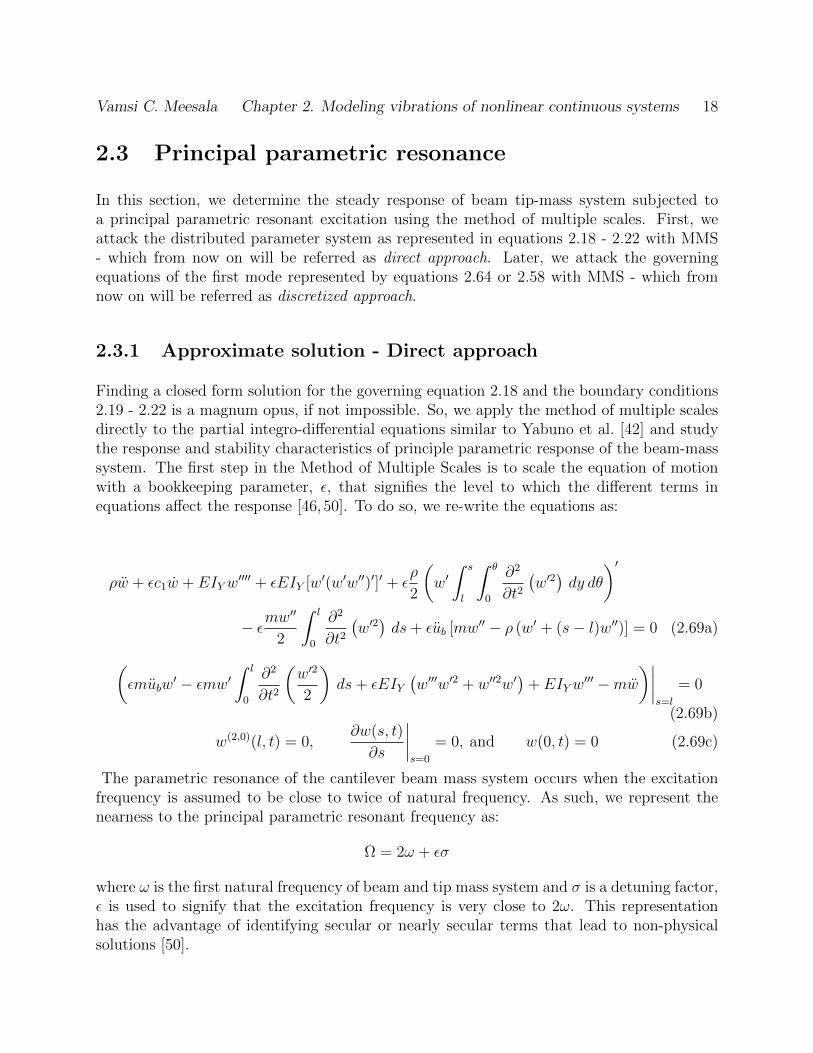
2.3 Principal parametric resonance
In this section, we determine the steady response of beam tip-mass system subjected toa principal parametric resonant excitation using the method of multiple scales. First, weattack the distributed parameter system as represented in equations 2.18 - 2.22 with MMS- which from now on will be referred as direct approach. Later, we attack the governingequations of the first mode represented by equations 2.64 or 2.58 with MMS - which fromnow on will be referred as discretized approach.
2.3.1 Approximate solution - Direct approach
Finding a closed form solution for the governing equation 2.18 and the boundary conditions2.19 - 2.22 is a magnum opus, if not impossible. So, we apply the method of multiple scalesdirectly to the partial integro-differential equations similar to Yabuno et al. [42] and studythe response and stability characteristics of principle parametric response of the beam-masssystem. The first step in the Method of Multiple Scales is to scale the equation of motionwith a bookkeeping parameter, ε, that signifies the level to which the different terms inequations affect the response [46,50]. To do so, we re-write the equations as:
ρw + εc1w + EIYw′′′′ + εEIY [w′(w′w′′)′]′ + ε
ρ
2
(w′∫ s
l
∫ θ
0
∂2
∂t2(w′2)dy dθ
)′− εmw
′′
2
∫ l
0
∂2
∂t2(w′2)ds+ εub [mw′′ − ρ (w′ + (s− l)w′′)] = 0 (2.69a)
(εmubw
′ − εmw′∫ l
0
∂2
∂t2
(w′2
2
)ds+ εEIY
(w′′′w′2 + w′′2w′
)+ EIYw
′′′ −mw)∣∣∣∣
s=l
= 0
(2.69b)
w(2,0)(l, t) = 0,∂w(s, t)
∂s
∣∣∣∣s=0
= 0, and w(0, t) = 0 (2.69c)
The parametric resonance of the cantilever beam mass system occurs when the excitationfrequency is assumed to be close to twice of natural frequency. As such, we represent thenearness to the principal parametric resonant frequency as:
Ω = 2ω + εσ
where ω is the first natural frequency of beam and tip mass system and σ is a detuning factor,ε is used to signify that the excitation frequency is very close to 2ω. This representationhas the advantage of identifying secular or nearly secular terms that lead to non-physicalsolutions [50].
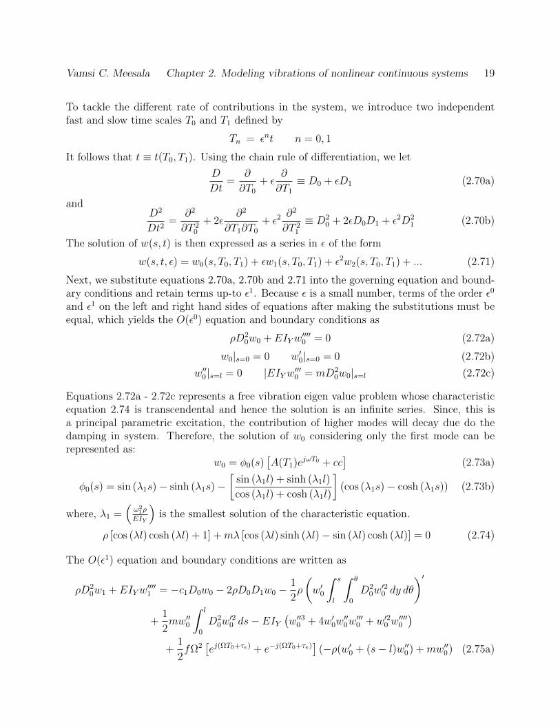
Vamsi C. Meesala Chapter 2. Modeling vibrations of nonlinear continuous systems 19
To tackle the different rate of contributions in the system, we introduce two independentfast and slow time scales T0 and T1 defined by
Tn = εnt n = 0, 1
It follows that t ≡ t(T0, T1). Using the chain rule of differentiation, we let
D
Dt=
∂
∂T0
+ ε∂
∂T1
≡ D0 + εD1 (2.70a)
andD2
Dt2=
∂2
∂T 20
+ 2ε∂2
∂T1∂T0
+ ε2∂2
∂T 21
≡ D20 + 2εD0D1 + ε2D2
1 (2.70b)
The solution of w(s, t) is then expressed as a series in ε of the form
w(s, t, ε) = w0(s, T0, T1) + εw1(s, T0, T1) + ε2w2(s, T0, T1) + ... (2.71)
Next, we substitute equations 2.70a, 2.70b and 2.71 into the governing equation and bound-ary conditions and retain terms up-to ε1. Because ε is a small number, terms of the order ε0
and ε1 on the left and right hand sides of equations after making the substitutions must beequal, which yields the O(ε0) equation and boundary conditions as
ρD20w0 + EIYw
′′′′0 = 0 (2.72a)
w0|s=0 = 0 w′0|s=0 = 0 (2.72b)
w′′0 |s=l = 0 |EIYw′′′0 = mD20w0|s=l (2.72c)
Equations 2.72a - 2.72c represents a free vibration eigen value problem whose characteristicequation 2.74 is transcendental and hence the solution is an infinite series. Since, this isa principal parametric excitation, the contribution of higher modes will decay due do thedamping in system. Therefore, the solution of w0 considering only the first mode can berepresented as:
w0 = φ0(s)[A(T1)ejωT0 + cc
](2.73a)
φ0(s) = sin (λ1s)− sinh (λ1s)−[
sin (λ1l) + sinh (λ1l)
cos (λ1l) + cosh (λ1l)
](cos (λ1s)− cosh (λ1s)) (2.73b)
where, λ1 =(ω21ρ
EIY
)is the smallest solution of the characteristic equation.
ρ [cos (λl) cosh (λl) + 1] +mλ [cos (λl) sinh (λl)− sin (λl) cosh (λl)] = 0 (2.74)
The O(ε1) equation and boundary conditions are written as
ρD20w1 + EIYw
′′′′1 = −c1D0w0 − 2ρD0D1w0 −
1
2ρ
(w′0
∫ s
l
∫ θ
0
D20w′20 dy dθ
)′+
1
2mw′′0
∫ l
0
D20w′20 ds− EIY
(w′′30 + 4w′0w
′′0w′′′0 + w′20 w
′′′′0
)+
1
2fΩ2
[ej(ΩT0+τe) + e−j(ΩT0+τe)
](−ρ(w′0 + (s− l)w′′0) +mw′′0) (2.75a)
Vamsi C. Meesala Chapter 2. Modeling vibrations of nonlinear continuous systems 20
w1|s=0 = 0 w′1|s=0 = 0 w′′1 |s=l = 0 (2.75b)
∣∣∣∣−mD20w0 + EIYw
′′′0 = 2mD0D1w0 +
1
2fmΩ2w′0
[ej(ΩT0+τe) + e−j(ΩT0+τe)
]+
1
2mw′0
∫ l
0
D20w′20 ds− EIY (w′0w
′′20 + w′20 w
′′′0 )
∣∣∣∣s=l
(2.75c)
The solution of w1 free of secular terms can be represented as:
w1(s, T0, T1) = φ1(s, T1)ejωT0 + c.c (2.76)
To identify secular terms and yield the solvability conditions, we multiply and integrate theequation 2.75a with e−jωT0 . This treatment will retain only the secular terms in the equation2.75a. Using Ω = 2ω + εσ and εT0 = T1, we re-write the O(ε) equations as
− ρω2φ1 + EIY φ′′′′1 = −jωAc1φ0 − 2jρωφ0A
′ + 2ω2ρA2A
(φ′0
∫ s
l
∫ θ
0
φ′20 dy dθ
)′− 2mω2A2Aφ′′0
∫ l
0
φ′20 ds− 3EIYA2A(φ′′30 + 4φ′0φ
′′0φ′′′0 + φ′20 φ
′′′′0
)+
1
2f(2ω + εσ)2ej(σT1+τe)A (−ρ(φ′0 + (s− l)φ′′0) +mφ′′0) ≡ H1 (2.77a)
φ1(0) = 0 φ′1(0) = 0 φ′′1(l) = 0 (2.77b)
∣∣∣∣mω2φ1 + EIY φ′′′1 = 2jmωφ′0A
′ +1
2fm(2ω + εσ)2ej(σT1+τe)Aφ′0
−2mω2A2Aφ′0
∫ l
0
φ′20 ds− 3EIYA2Aφ′0(φ′′20 + φ′0φ
′′′0 )
∣∣∣∣s=l
≡ H2 (2.77c)
Next, we multiply an adjoint solution, u(s), which will be specified later, by equation 2.77aand integrate it over the domain, which yields∫ l
0
(−ρω2φ1 + EIY φ′′′′1 )u ds =
∫ l
0
H1u ds (2.78a)
using integration by parts, the integrals are transferred to u as,∫ l
0
(−ρω2u+ EIY u′′′′)φ1 ds+ [EIY φ
′′′1 u− EIY φ′′1u′ + EIY φ
′1u′′ − EIY φ1u
′′′]s=ls=0 =
∫ l
0
H1u ds
(2.78b)The adjoint equation of the homogeneous equation of 2.77a (H1=0) is defined as the coeffi-cient of φ1 in the integrand on left-hand side as:
− ρω2u+ EIY u′′′′ = 0 (2.78c)
Vamsi C. Meesala Chapter 2. Modeling vibrations of nonlinear continuous systems 21
Considering the homogeneous boundary conditions in equations 2.77b, 2.77c and 2.78c(H2=0), equation 2.78b can simplified to[
−(mω2u+ EIY u′′′)φ1 + EIY φ
′1u′′]s=l− [EIY φ
′′′1 u− EIY φ′′1u′]s=0 = 0 (2.78d)
The available boundary conditions don’t provide any information about φ1(l), φ′1(l), φ′′′1 (0)and φ′′1(0). Nevertheless, irrespective of their values, equation 2.78d should be uniquelysatisfied. This imposes the boundary condition on the adjoint solution as:
u(0) = 0 u′(0) = 0 u′′(l) = 0 (2.78e)
[mω2u+ EIY u′′′]s=l = 0 (2.78f)
From the adjoint system represented by the equations 2.78c, 2.78e and 2.78f and homo-geneous O(ε1) system, it can be said that the O(ε1) equations are a self-adjoint system.Equations 2.78c, 2.78e and 2.78f are identical to O(ε) equations, therefore, the non-trivialsolution of the adjoint system is:
u(s) = φ0(s) (2.79)
Because the homogeneous system has a non-trivial solution, the non-homogeneous systemrequires a solvability condition for determined the solution [46], which is determined asfollows. Using the well-defined adjoint system from equations 2.78c - 2.78f and consideringthe actual boundary conditions of φ1, equation 2.78b can be re-written as:∫ l
0
H1φ0 ds = H2φ0(l) (2.80a)
∫ l
0
[−jωAc1φ0 − c2g1φ
20 − 2jρωφ0A
′ + 2ω2ρA2A
(φ′0
∫ s
l
∫ θ
0
φ′20 dy dθ
)′−2mω2A2Aφ′′0
∫ l
0
φ′20 ds− 3EIYA2A(φ′′30 + 4φ′0φ
′′0φ′′′0 + φ′20 φ
′′′′0
)+
1
2f(2ω + εσ)2ej(σT1+τe)A (−ρ(φ′0 + (s− l)φ′′0) +mφ′′0)
]φ0 ds = φ0 [2jmωφ0A
′
+1
2fm(2ω + εσ)2ej(σT1+τe)Aφ′0 − 2mω2A2Aφ′0
∫ l
0
φ′20 ds− 3EIYA2Aφ′20 φ
′′′0
]∣∣∣∣s=l
(2.80b)
Using the polar representation of A, as A(T1) = 12a(T1)ejβ(T1), equation 2.80b can be simpli-
Vamsi C. Meesala Chapter 2. Modeling vibrations of nonlinear continuous systems 22
fied as:∫ l
0
[−1
2jωac1φ0 − jρωφ0 (a′ + jβ′a) +
1
4ω2ρa3
(φ′0
∫ s
l
∫ θ
0
φ′20 dy dθ
)′−1
4mω2a3φ′′0
∫ l
0
φ′20 ds−3
8EIY a
3(φ′′30 + 4φ′0φ
′′0φ′′′0 + φ′20 φ
′′′′0
)+
1
4f(2ω + εσ)2ej(σT1+τe)ae−2jβ (−ρ(φ′0 + (s− l)φ′′0) +mφ′′0)
]φ0 ds = φ0 [jmωφ0 (a′ + jβ′a)
+1
4fm(2ω + εσ)2ej(σT1+τe)ae−2jβφ′0 −
1
4mω2a3φ′0
∫ l
0
φ′20 ds−3
8EIY a
3φ′20 φ′′′0
]∣∣∣∣s=l
(2.81)
Separating the real and imaginary parts yields
aβ′[∫ l
0
ρωφ20 ds+mωφ0(l)2
]= a3
[−∫ l
0
1
4ω2ρ
(φ′0
∫ s
l
∫ θ
0
φ′20 dy dθ
)′φ0 ds
+
∫ l
0
1
4mω2φ′′0
(∫ l
0
φ′20 ds
)φ0 ds+
3
8
∫ l
0
EIY (φ′0(φ′0φ′′0)′)′φ0 ds−
1
4mω2φ0(l)φ′0(l)
(∫ l
0
φ′20 ds
)−3
8EIY φ0(l)φ′20 (l)φ′′′0 (l)
]+
1
4af(2ω+εσ)2 cos(σT1+τe−2β)
[∫ l
0
(ρ[φ′0 + (s− l)φ′′0]−mφ′′0)φ0 ds
+mφ0(l)φ′0(l)] (2.82a)
a′ω
[−∫ l
0
ρφ20 ds−mφ0(l)2
]=
1
2aωc1
(∫ l
0
φ20 ds
)+
1
4af(2ω + εσ)2 sin(σT1 + τe − 2β)
[∫ l
0
(ρ[φ′0 + (s− l)φ′′0]−mφ′′0)φ0 ds+mφ0(l)φ′0(l)
](2.82b)
Defining
γ = σT1 + τe − 2β =⇒ D1β =1
2[−D1γ + σ]
µ1D =1
2
c1
∫ l0φ2
0 ds∫ l0ρφ2
0 ds+mφ0(l)2
αD =
∫ l0EIY (φ′0(φ′0φ
′′0)′)′φ0 ds− EIY φ0(l)φ′20 (l)φ′′′0 (l)∫ l0ρφ2
0 ds+mφ0(l)2=−∫ l
0EIY φ
′20 (φ′0φ
′′0)′ ds∫ l
0ρφ2
0 ds+mφ0(l)2
δD =ρ∫ l
0
(φ′0∫ sl
∫ θ0φ′20 dy dθ
)′φ0 ds−m
[∫ l0φ′′0
(∫ l0φ′20 ds
)φ0 ds− φ0(l)φ′0(l)
(∫ l0φ′20 ds
)]∫ l
0ρφ2
0 ds+mφ0(l)2
Vamsi C. Meesala Chapter 2. Modeling vibrations of nonlinear continuous systems 23
which can be re-written as
δD =ρ∫ l
0φ′20
(∫ ls
∫ θ0φ′20 dy dθ
)ds+m
(∫ l0φ′20 ds
)2
∫ l0ρφ2
0 ds+mφ0(l)2
and
ηD =−(2ω + εσ)2
[∫ l0
(ρ[φ′0 + (s− l)φ′′0]−mφ′′0)φ0 ds+mφ0(l)φ′0(l)]
∫ l0ρφ2
0 ds+mφ0(l)2
which can be re-written as
ηD =−(2ω + εσ)2
[ρ∫ l
0(l − s)φ′20 ds+m
∫ l0φ′20 ds
]∫ l
0ρφ2
0 ds+mφ0(l)2
yields the amplitude and phase modulation equations as:
a
(σω
2− 1
2ωγ′)− a3
(3αD
8− δDω
2
4
)= −1
4afηD cos(γ) (2.83a)
ωa′ + aµ1Dω =1
4afηD sin(γ) (2.83b)
and the approximate solution is given by
w(s, t) ≈ 1
2φ0(s)ae
12j(Ωt+τe−γ) + ... (2.84)
2.3.2 Approximate solution - Discretized approach
Next, we tackle the discretized equation of the first mode determined in the previous section2.2.4 with the method of multiple scales. To this end, we scale equations 2.64 in a similarway to the equation 2.69 and write
q + ω2q + 2εµ1q + εδq(q2 + qq) + εαq3 = εηqf cos(Ωt+ τe) (2.85)
Using the same time scales defined in section 2.3.1 and expressing the solution of q(t) is thenexpressed as a series in ε of the form
q(t, ε) = q0(T0, T1) + εq1(T0, T1) + ε2q2(T0, T1) + ... (2.86)
we obtain the order ε0 and ε1 equations as:O(ε0) equation
D20q0 + q0ω
2 = 0 , and (2.87)
Vamsi C. Meesala Chapter 2. Modeling vibrations of nonlinear continuous systems 24
O(ε1) equation
D20q1 + q1ω
2 = −δq0 (D0q0)2 − δq20D
20q0 − 2µ1D0q0 − 2D0D1q0 − αq3
0
+1
2fηq0e
iτe+iT0Ω +1
2fηq0e
−iτe−iT0Ω (2.88)
The solution of linear differential equation 2.87 is of the form:
q0 = A(T1)ejωT0 + A(T1)e−jωT0 = A(T1)ejωT0 + cc (2.89)
Using this solution, we rewrite the different terms that contain q0 in equation 2.88 as
−δq0 (D0q0)2 = δω2A3e3jT0ω − δω2A2AejT0ω + cc
−δq20D
20q0 = δω2A3e3jT0ω + 3δω2A2AejT0ω + cc
−2µ1 (D0q0) = −2jωAµ1ejT0ω + cc
−2 (D0D1q0) = −2jωA′ejT0ω + cc
−αq30 = −αA3e3jωT0 − 3ejT0ωαA2A+ cc
Using Ω = 2ω + εσ, the excitation terms are written as
1
2fηq0e
jτe+iT0Ω +1
2fηq0e
−jτe−iT0Ω =1
2fηAe−jσT1−jωT0−jτe +
1
2fηAejσT1+3jωT0+jτe + cc
Because the solution is assumed to be periodic, the sum of all secular terms, which leadto non-periodic solutions, is equated to zero. To this end, upon substituting the aboveexpansions into the equation 2.88, we obtain
− 3A2αA+1
2ejσT1+jτefηA+ 2A2δω2A− 2jωD1A− 2jAωµ1 = 0, and (2.90)
− 3A2αA+1
2e−jσT1−jτefηA+ 2Aδω2A2 + 2jωD1A+ 2jAωµ1 = 0 (2.91)
These two equations provide valuable information about D1A and D1A that can be usedto study the progression of the amplitude of the response in time. The two equations arecomplex conjugates to each other, so satisfying one equation will automatically satisfy theother.
Substituting 12aejβ for A and 1
2ae−jβ for A into equation 2.90 yields,
− 2jω
(1
2a′ +
1
2jaβ′
)− 3
8αa3 +
1
4a3δω2 − jaµ1ω +
1
4afηejγ − g1µ2 = 0 (2.92)
Vamsi C. Meesala Chapter 2. Modeling vibrations of nonlinear continuous systems 25
where −2β(T1) + τe + σT1 is replaced by γ(T1) to remove the explicit dependence on T1.Therefore, β′(T1) = 1
2[−γ′(T1) + σ]. Substituting for the value of β′ and separating the real
and imaginary parts, we obtain the amplitude and phase modulation equations as
a
(σω
2− 1
2ωγ′)− a3
(3α
8− δω2
4
)= −1
4afη cos(γ) (2.93a)
ωa′ + aµ1ω =1
4afη sin(γ) (2.93b)
It is noted that the parameters µ1,α,δ,η defined above are equivalent to µ1D,αD,δD,ηD usedin the section 2.3.1. Therefore, amplitude and phase modulation equations 2.83a and 2.83bderived using direct method by determining solvability conditions are identical to amplitudeand phase modulation equations 2.93a and 2.93b derived using the Galerkin discretizationand by considering nonlinear boundary conditions. This re-affirms the importance of con-sidering the nonlinear boundary conditions while applying modal analysis.
The steady state equations are obtained by setting a = 0 and γ = 0 in equations 2.93a and2.93b. Squaring and adding these equations yields a relation between the amplitude of theresponse, a, and the system’s parameters as a function of the detuning parameter, σ, andthe amplitude of the response f . By squaring and adding the , we obtain the amplituderesponse function [
σω
2+ a2
(−3α
8+δω2
4
)]2
+ ω2µ21 =
η2f 2
16(2.94)
2.4 Results and discussion
In this section, we evaluate the importance of considering and neglecting nonlinear boundaryconditions while developing the discretized governing equations.
2.4.1 Linear vs non-linear boundary conditions
Comparing equations 2.59 - 2.61 with equations 2.66 - 2.68, we note assuming linearizedboundary conditions has resulted in additional terms for the forces related to geometricnonlinearities, inertial nonlinearities and the external excitation. As will be shown below, theoptions of considering or not considering these terms yield significantly differing responses.To emphasize this, we consider a carbon fiber/epoxy resin composite beam and tip masssystem with the physical properties listed in Table 2.1.
Vamsi C. Meesala Chapter 2. Modeling vibrations of nonlinear continuous systems 26
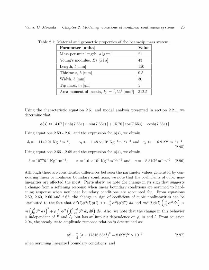
Table 2.1: Material and geometric properties of the beam-tip mass system.
Parameter [units] Value
Mass per unit length, ρ [g/m] 21
Young’s modulus, E) [GPa] 43
Length, l [mm] 150
Thickness, h [mm] 0.5
Width, b [mm] 30
Tip mass, m [gm] 5
Area moment of inertia, IY = 112bh3 [mm4] 312.5
Using the characteristic equation 2.51 and modal analysis presented in section 2.2.1, wedetermine that
φ(s) ≈ 14.67 [ sinh(7.55s)− sin(7.55s) ] + 15.76 [ cos(7.55s)− cosh(7.55s) ]
Using equations 2.59 - 2.61 and the expression for φ(s), we obtain
δl ≈ −1149.91 Kg−1m−2, αl ≈ −1.48× 10⁷ Kg−1m−2s−2, and ηl ≈ −16.91Ω2 m−1s−2
(2.95)Using equations 2.66 - 2.68 and the expression for φ(s), we obtain
δ ≈ 10776.1 Kg−1m−2, α ≈ 1.6× 10⁷ Kg−1m−2s−2, and η ≈ −8.31Ω2 m−1s−2 (2.96)
Although there are considerable differences between the parameter values generated by con-sidering linear or nonlinear boundary conditions, we note that the coefficients of cubic non-linearities are affected the most. Particularly we note the change in its sign that suggestsa change from a softening response when linear boundary conditions are assumed to hard-ening response when nonlinear boundary conditions are accounted for. From equations2.59, 2.60, 2.66 and 2.67, the change in sign of coefficient of cubic nonlinearities can be
attributed to the fact that φ′′′(l)φ′2(l)φ(l) <<∫ l
0φ′2(φ′φ′′)′ ds and mφ′(l)φ(l)
(∫ l0φ′2 ds
)>
m(∫ l
0φ′2 ds
)2
+ ρ∫ l
0φ′2(∫ l
s
∫ θ0φ′2 dy dθ
)ds. Also, we note that the change in this behavior
is independent of E and IY but has an implicit dependence on ρ, m and l. From equation2.94, the steady state amplitude response relation is determined as:
µ21 +
1
4
(σ + 17316.63a2
)2= 8.6Ω2f 2 × 10⁻³ (2.97)
when assuming linearized boundary conditions, and
Vamsi C. Meesala Chapter 2. Modeling vibrations of nonlinear continuous systems 27
µ21 +
1
4
(σ − 217475.36a2
)2= 2.07Ω2f 2 × 10⁻³ (2.98)
when the nonlinearities are accounted for in the boundary conditions.
4 4.2 4.4 4.6 4.8 5 5.20
200
400
600
800
1000 Nonlinear boundary conditionsLinear boundary conditions
(a)
4 4.2 4.4 4.6 4.8 5 5.20
100
200
300
400
500Nonlinear boundary conditionsLinear boundary conditions
(b)
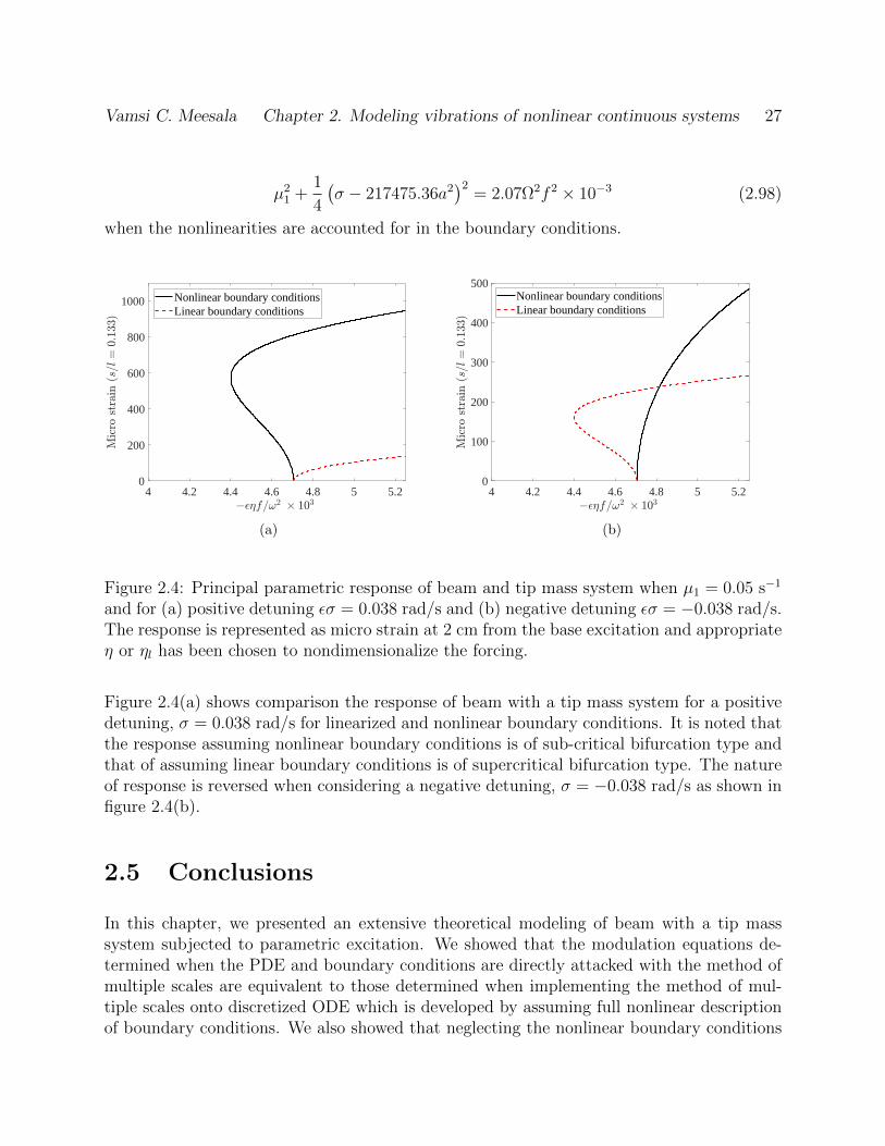
Figure 2.4: Principal parametric response of beam and tip mass system when µ1 = 0.05 s−1
and for (a) positive detuning εσ = 0.038 rad/s and (b) negative detuning εσ = −0.038 rad/s.The response is represented as micro strain at 2 cm from the base excitation and appropriateη or ηl has been chosen to nondimensionalize the forcing.
Figure 2.4(a) shows comparison the response of beam with a tip mass system for a positivedetuning, σ = 0.038 rad/s for linearized and nonlinear boundary conditions. It is noted thatthe response assuming nonlinear boundary conditions is of sub-critical bifurcation type andthat of assuming linear boundary conditions is of supercritical bifurcation type. The natureof response is reversed when considering a negative detuning, σ = −0.038 rad/s as shown infigure 2.4(b).
2.5 Conclusions
In this chapter, we presented an extensive theoretical modeling of beam with a tip masssystem subjected to parametric excitation. We showed that the modulation equations de-termined when the PDE and boundary conditions are directly attacked with the method ofmultiple scales are equivalent to those determined when implementing the method of mul-tiple scales onto discretized ODE which is developed by assuming full nonlinear descriptionof boundary conditions. We also showed that neglecting the nonlinear boundary conditions
Vamsi C. Meesala Chapter 2. Modeling vibrations of nonlinear continuous systems 28
while developing the discretized governing equation of temporal modes can significantly alterthe response. In particular, we demonstrated that for the problem under consideration, thesign of the cubic nonlinearity coefficients are opposite to the one obtained when assuminglinearized boundary conditions are neglected to that of when considered. From figure 2.4(a)and 2.4(b) we showed that, nature of Hopf bifurcation is exactly opposite and the amplitudesof response are considerably different when considering linearized and nonlinear boundaryconditions. From the analysis and results discussed in this chapter, it can be concluded that,though neglecting nonlinear boundary conditions can simplify the math in determining thegoverning equations, the representation of response can be significantly altered.
Chapter 3
Parameter sensitivity of cantileverbeam with tip mass to parametricexcitation
The cantilever beam with a tip mass configuration has been used to model robotic arms[6,7], antenna masts [8,9], wings with store configurations [10–15], energy harvesting devices[16–22], vibrating beam gyroscopes [23,24] and bio/chemical sensors [25–31]. In all of theseapplications, there is a need for matching the system’s response with a predicted valuein order to determine a quantity of interest. For instance, in a bio/chemical sensor, theobjective would be to detect the presence of target bio-materials by assessing a very smallchange in the static or dynamic response of the beam-mass system caused by the binding ofthe bio-material mass to the beam. In the static response, the bending or deflection of thebeam is related to the value of the additional mass. In the dynamic resonant response, thepresence of the added mass is detected by measuring a shift in the resonance frequency of thecantilever beam. Although the analysis seems straightforward, determining the resonancefrequency may require additional evaluation because the dynamic resonant response dependson small variations in the beam’s dimensions, material properties, operational conditionssuch as environmental thermal effects, and fatigue induced by cyclic loading. Subsequently,any uncertainty in the beam’s dimensions, the mass value or material properties can resultin inaccurate estimates of the natural frequency, which may induce discrepancies betweenthe proposed cantilever beam-mass model and predicted values and experimental results,thereby compromising the fidelity of the model representing the device.
The effects of discrepancies in representative parameters on the response of a beam masssystem can be quantified by performing a sensitivity analysis of the response to variations inthese parameters. Alternatively, one may think of exploiting these effects in order to detectchanges in the parameters that can be associated with additional mass and manufacturingor operational conditions such as the ones discussed above. The sensitivity analysis becomes
29
Vamsi C. Meesala Chapter 3. Sensitivity Analysis 30
more challenging in applications where nonlinear effects cannot be neglected or are of pri-mary interest. For example in the case of the bio mass sensor, Younis and Nayfeh [51] notedthat accurate frequency response requires accurate representation of the nonlinearities of anelectrically actuated micro beam subjected to axial loading. Zhang et al. [30] and Zhangand Turner [31] showed that the jump phenomenon in the principal parametric resonanceof a micro cantilever can be utilized for mass sensing with significantly higher sensing ca-pability in comparison to linear resonant type sensors. Often, when considering a nonlinearresponse, the type and point of bifurcation are highly sensitive to the system’s nonlinearities.Perturbation analysis around this point provides a capability to assess the sensitivity of theresponse to small variations in the model parameters.
In this chapter, we consider a cantilever beam with a tip mass under parametric excitationand use the mathematical model developed in chapter 2 to assess its nonlinear response andperform sensitivity analysis of the nonlinear response to variations in the elasticity (stiff-ness) and additional mass of the beam and tip mass system. Using a discretized form ofthe governing equation, we evaluate this sensitivity by implementing the Method of Mul-tiple Scales [46, 50]. We choose the discretized equation as the analysis is more intuitivein comparison to the direct approach, which involves solving five nonlinear integro-partialdifferential equations. Particular attention is paid to determining the effects of varying thesystem’s parameter on changing the type of bifurcation under different resonance conditions.Although nonlinear and damping terms in the governing equation are of O(ε) and hence onecould assume that a solution considering the modulation equations up to O(ε) is appropriate,the small uncertainties in the nonlinear parameter are of the order O(ε2) in the governingequation, which requires a solution considering the modulation equations up to O(ε2). Tobe consistent and identify the sensitivity of the response from equilibrium solution, we willcompare the O(ε2) solutions for the governing equations with and without small variationsin their parameters.
3.1 Governing equations
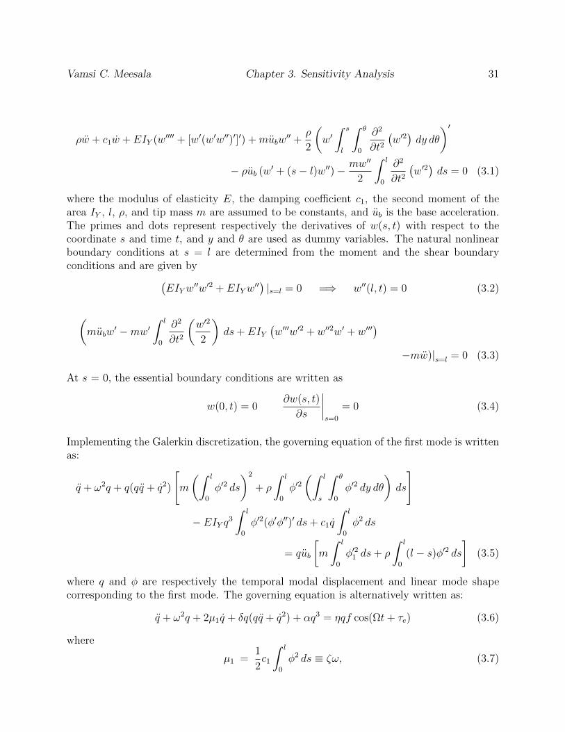
A schematic of the cantilever beam with a tip mass subjected to parametric excitation ispresented in figure 3.1. The beam with length l, width b, thickness h, and mass per unitlength ρ, is clamped at the base where it is subjected to a harmonic excitation at twice itsnatural frequency. Assuming that the beam is in-extensible and that the Euler-Bernoullibeam theory is applicable the governing equation, derived in chapter 2, is written as
Vamsi C. Meesala Chapter 3. Sensitivity Analysis 31
ρw + c1w + EIY (w′′′′ + [w′(w′w′′)′]′) +mubw′′ +
ρ
2
(w′∫ s
l
∫ θ
0
∂2
∂t2(w′2)dy dθ
)′− ρub (w′ + (s− l)w′′)− mw′′
2
∫ l
0
∂2
∂t2(w′2)ds = 0 (3.1)
where the modulus of elasticity E, the damping coefficient c1, the second moment of thearea IY , l, ρ, and tip mass m are assumed to be constants, and ub is the base acceleration.The primes and dots represent respectively the derivatives of w(s, t) with respect to thecoordinate s and time t, and y and θ are used as dummy variables. The natural nonlinearboundary conditions at s = l are determined from the moment and the shear boundaryconditions and are given by(
EIYw′′w′2 + EIYw
′′) |s=l = 0 =⇒ w′′(l, t) = 0 (3.2)
(mubw
′ −mw′∫ l
0
∂2
∂t2
(w′2
2
)ds+ EIY
(w′′′w′2 + w′′2w′ + w′′′
)−mw)|s=l = 0 (3.3)
At s = 0, the essential boundary conditions are written as
w(0, t) = 0∂w(s, t)
∂s
∣∣∣∣s=0
= 0 (3.4)
Implementing the Galerkin discretization, the governing equation of the first mode is writtenas:
q + ω2q + q(qq + q2)
[m
(∫ l
0
φ′2 ds
)2
+ ρ
∫ l
0
φ′2(∫ l
s
∫ θ
0
φ′2 dy dθ
)ds
]
− EIY q3
∫ l
0
φ′2(φ′φ′′)′ ds+ c1q
∫ l
0
φ2 ds
= qub
[m
∫ l
0
φ′21 ds+ ρ
∫ l
0
(l − s)φ′2 ds]
(3.5)
where q and φ are respectively the temporal modal displacement and linear mode shapecorresponding to the first mode. The governing equation is alternatively written as:
q + ω2q + 2µ1q + δq(qq + q2) + αq3 = ηqf cos(Ωt+ τe) (3.6)
where
µ1 =1
2c1
∫ l
0
φ2 ds ≡ ζω, (3.7)
Vamsi C. Meesala Chapter 3. Sensitivity Analysis 32
Z
x
ub(t)
sl
w(s, t)
um=u(l,t)
p1
p1'dw
ds
ds
du
α(s)
ρ
m
h
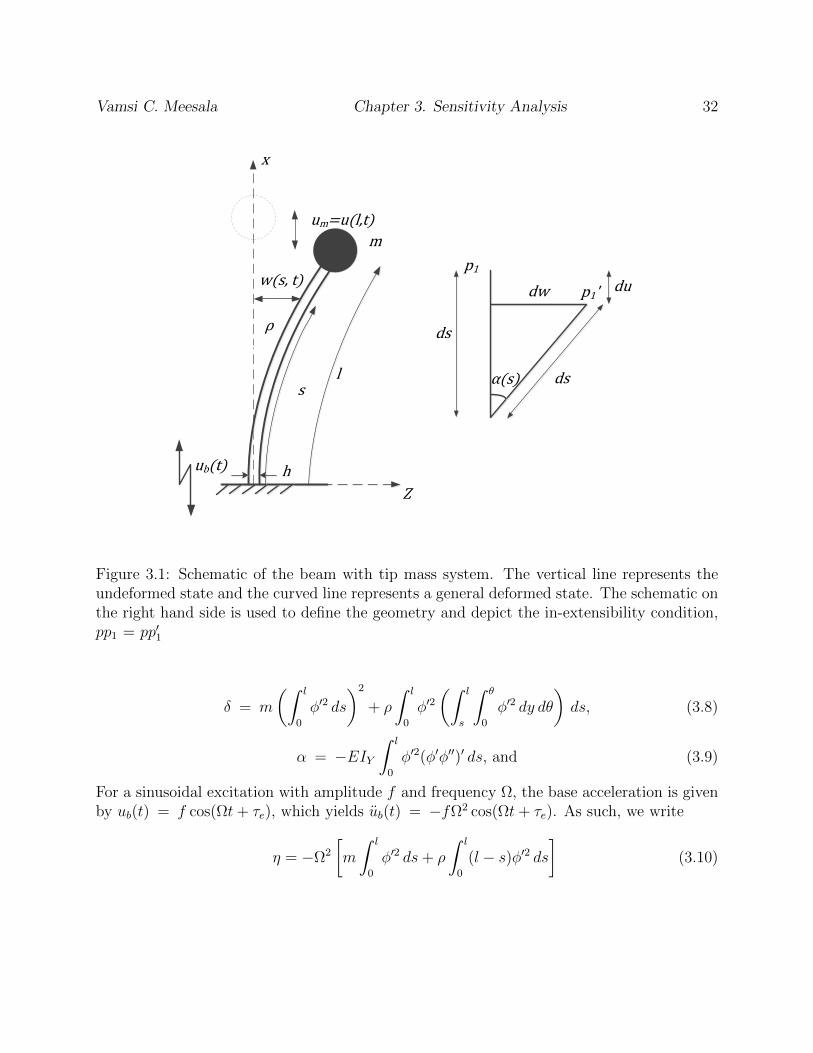
Figure 3.1: Schematic of the beam with tip mass system. The vertical line represents theundeformed state and the curved line represents a general deformed state. The schematic onthe right hand side is used to define the geometry and depict the in-extensibility condition,pp1 = pp′1
δ = m
(∫ l
0
φ′2 ds
)2
+ ρ
∫ l
0
φ′2(∫ l
s
∫ θ
0
φ′2 dy dθ
)ds, (3.8)
α = −EIY∫ l
0
φ′2(φ′φ′′)′ ds, and (3.9)
For a sinusoidal excitation with amplitude f and frequency Ω, the base acceleration is givenby ub(t) = f cos(Ωt+ τe), which yields ub(t) = −fΩ2 cos(Ωt+ τe). As such, we write
η = −Ω2
[m
∫ l
0
φ′2 ds+ ρ
∫ l
0
(l − s)φ′2 ds]
(3.10)
Vamsi C. Meesala Chapter 3. Sensitivity Analysis 33
3.2 Sensitivity analysis
Next, we employ the method of multiple scales to determine the approximate solution and tostudy the stability characteristics of the response governed by equation 3.6 when subjectedto small variations in elasticity and tip mass. First, we investigate the principal parametricresonance response characteristics of the beam tip mass system without any variations inits parameters by appropriately scaling contributions of the different terms in the governingequation 3.6 as:
q + ω2q + 2εµ1q + εδq(q2 + qq
)+ εαq3 = εηqf cos(Ωt+ τe) (3.11)
where the forcing frequency is given by Ω = 2ω + εσ. Here, εσ is a small detuning param-eter that quantifies the difference between the excitation frequency and twice the naturalfrequency of the first mode of the beam and tip mass system.
As discussed above, any small uncertainty in the nonlinear parameters due to variations inelasticity and tip mass is of order O(ε2) in the governing equation 3.11, which requires thederivation of the modulation equations up to O(ε2) to capture their influence. As such, wefirst compare the approximate solutions and response functions of the original system, withno parameter variations, when implementing O(ε) and O(ε2) approximations.
3.2.1 Approximate solution
To obtain an approximate solution using the method of multiple scales, we introduce threeindependent time scales T0, T1 and T2 defined by
Tn = εnt n = 0, 1, 2
Using the chain rule of differentiation, we expand the derivatives up to O(ε2) and write:
D
Dt=
∂
∂T0
+ ε∂
∂T1
+ ε2∂
∂T2
≡ D0 + εD1 + ε2D2 (3.12a)
and
D2
Dt2=
∂2
∂T 20
+ 2ε∂2
∂T1∂T0
+ ε2(
2∂2
∂T0∂T2
+∂2
∂T 21
)≡ D2
0 + 2εD0D1
+ ε2(D2
1 + 2D0D2
)(3.12b)
The solution of q(t) is then expressed as
q(t, ε) = q0(T0, T1, T2) + εq1(T0, T1, T2) + ε2q2(T0, T1, T2) + ... (3.13)
Vamsi C. Meesala Chapter 3. Sensitivity Analysis 34
Substituting equations 3.12a, 3.12b and 3.13 into the equation 3.11, retaining terms up-toO(ε2) and equating terms of the order ε0, ε1 and ε2 on the left and right hand sides of equa-tion 3.11, we obtain
ε0− order equation:D2
0q0 + q0ω2 = 0 , (3.14)
ε1− order equation:
D20q1 + q1ω
2 = −2D0D1q0 − δq0D0q20 − δq2
0D20q0 − δq0 (D0q0)2 − αq3
0 − 2µ1D0q0
+1
2fηq0e
iτe+iT0Ω +1
2fηq0e
−iτe−iT0Ω, and (3.15)
ε2− order equation:
D20q2 + q2ω
2 = −2D0D1q1 −D21q0 − 2D0D2q0 − 2δq0D0q0D0q1 − 2δq0D0q0D1q0
− δq1D0q20 − 2δq2
0D0D1q0 − δq1D0q20 − 2δq0q1D
20q0 − 3αq1q
20 − 2µ1D0q1 − 2µ1D1q0
+1
2fηq1e
iτe+iT0Ω +1
2fηq1e
−iτe−iT0Ω (3.16)
By eliminating the secular terms that result from substituting the solution of q0 from equa-tion 3.14 into the ε1-order equation 3.15, we obtain the amplitude and phase modulationequations as:
a = εfη
4ωa sin γ − εµ1a, and (3.17a)
γ = εσ + εfη
2ωcos γ − ε(3α− 2δω2)
4ωa2 (3.17b)
where the steady state equations are obtained by setting a = 0 and γ = 0. Squaringand adding these equations yields a relation between amplitude of the response, a, and thesystem’s parameters as a function of the detuning parameter, σ, and the amplitude of theresponse f .
µ21 +
[1
2σ − (3α− 2δω2)
8ωa2
]2
=f 2η2
16ω2(3.18)
Carrying the same procedure to the ε2−order, i.e., finding the solution of q1, and substitutingit in equation 3.16, we obtain the following amplitude and phase modulation equations
a = m11a sin γ +m21a3 sin γ +m31a
3 +m41a, and (3.19a)
γ = εσ −m12 cos γ −m22a2 cos γ −m32a
2 −m42 −m52a4 (3.19b)
where
m11 = −εfη(εσ − 2ω)
8ω2, m21 = −ε2fη(5α + 6δω2)
64ω3,
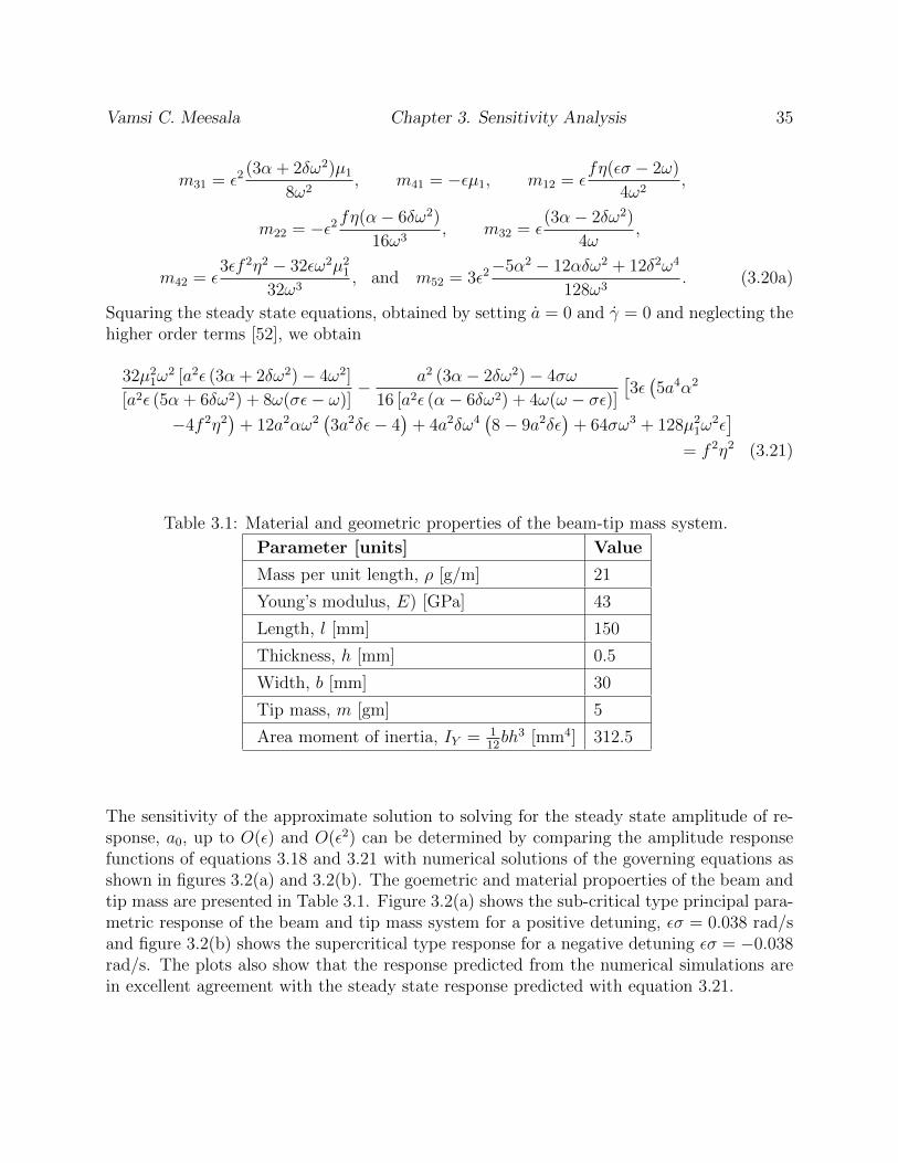
Vamsi C. Meesala Chapter 3. Sensitivity Analysis 35
m31 = ε2(3α + 2δω2)µ1
8ω2, m41 = −εµ1, m12 = ε
fη(εσ − 2ω)
4ω2,
m22 = −ε2fη(α− 6δω2)
16ω3, m32 = ε
(3α− 2δω2)
4ω,
m42 = ε3εf 2η2 − 32εω2µ2
1
32ω3, and m52 = 3ε2
−5α2 − 12αδω2 + 12δ2ω4
128ω3. (3.20a)
Squaring the steady state equations, obtained by setting a = 0 and γ = 0 and neglecting thehigher order terms [52], we obtain
32µ21ω
2 [a2ε (3α + 2δω2)− 4ω2]
[a2ε (5α + 6δω2) + 8ω(σε− ω)]− a2 (3α− 2δω2)− 4σω
16 [a2ε (α− 6δω2) + 4ω(ω − σε)][3ε(5a4α2
−4f 2η2)
+ 12a2αω2(3a2δε− 4
)+ 4a2δω4
(8− 9a2δε
)+ 64σω3 + 128µ2
1ω2ε]
= f 2η2 (3.21)
Table 3.1: Material and geometric properties of the beam-tip mass system.
Parameter [units] Value
Mass per unit length, ρ [g/m] 21
Young’s modulus, E) [GPa] 43
Length, l [mm] 150
Thickness, h [mm] 0.5
Width, b [mm] 30
Tip mass, m [gm] 5
Area moment of inertia, IY = 112bh3 [mm4] 312.5
The sensitivity of the approximate solution to solving for the steady state amplitude of re-sponse, a0, up to O(ε) and O(ε2) can be determined by comparing the amplitude responsefunctions of equations 3.18 and 3.21 with numerical solutions of the governing equations asshown in figures 3.2(a) and 3.2(b). The goemetric and material propoerties of the beam andtip mass are presented in Table 3.1. Figure 3.2(a) shows the sub-critical type principal para-metric response of the beam and tip mass system for a positive detuning, εσ = 0.038 rad/sand figure 3.2(b) shows the supercritical type response for a negative detuning εσ = −0.038rad/s. The plots also show that the response predicted from the numerical simulations arein excellent agreement with the steady state response predicted with equation 3.21.
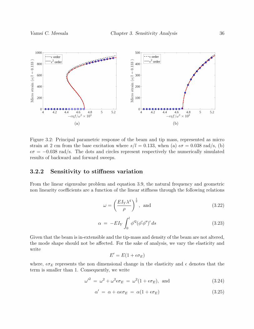
Vamsi C. Meesala Chapter 3. Sensitivity Analysis 36
4 4.2 4.4 4.6 4.8 5 5.20
200
400
600
800
1000 order2 order
(a)
4 4.2 4.4 4.6 4.8 5 5.20
100
200
300
400
500 order2 order
(b)
Figure 3.2: Principal parametric response of the beam and tip mass, represented as microstrain at 2 cm from the base excitation where s/l = 0.133, when (a) εσ = 0.038 rad/s, (b)εσ = −0.038 rad/s. The dots and circles represent respectively the numerically simulatedresults of backward and forward sweeps.
3.2.2 Sensitivity to stiffness variation
From the linear eigenvalue problem and equation 3.9, the natural frequency and geometricnon linearity coefficients are a function of the linear stiffness through the following relations
ω =
(EIY λ
4
ρ
) 12
, and (3.22)
α = −EIY∫ l
0
φ′2(φ′φ′′)′ ds (3.23)
Given that the beam is in-extensible and the tip-mass and density of the beam are not altered,the mode shape should not be affected. For the sake of analysis, we vary the elasticity andwrite
E ′ = E(1 + εσE)
where, εσE represents the non dimensional change in the elasticity and ε denotes that theterm is smaller than 1. Consequently, we write
ω′2
= ω2 + ω2εσE = ω2(1 + εσE), and (3.24)
α′ = α + αεσE = α(1 + εσE) (3.25)
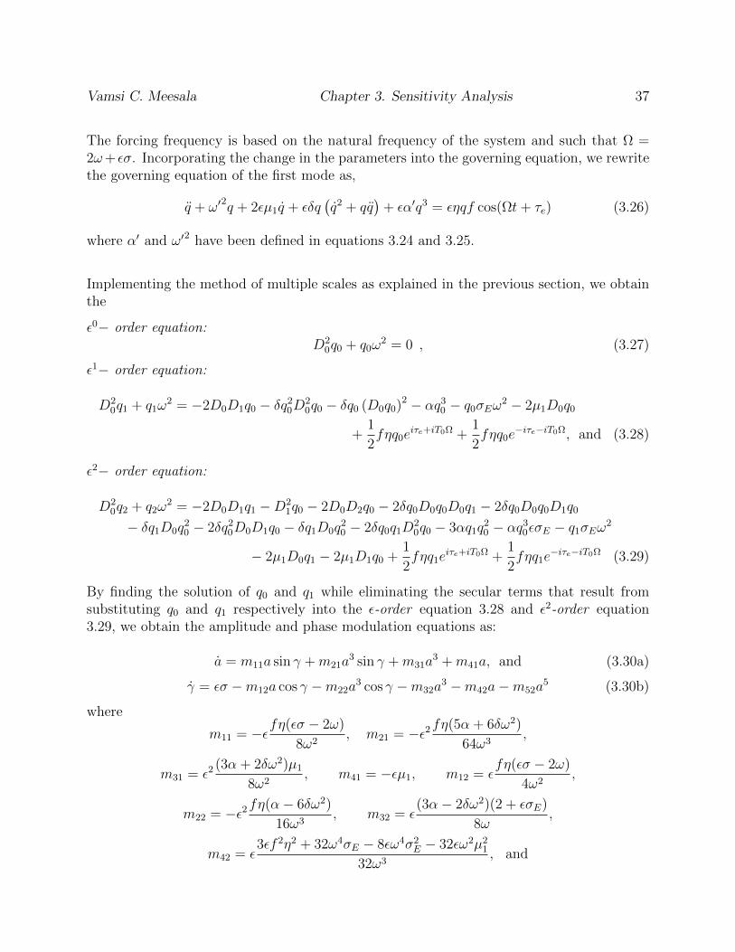
Vamsi C. Meesala Chapter 3. Sensitivity Analysis 37
The forcing frequency is based on the natural frequency of the system and such that Ω =2ω+ εσ. Incorporating the change in the parameters into the governing equation, we rewritethe governing equation of the first mode as,
q + ω′2q + 2εµ1q + εδq
(q2 + qq
)+ εα′q3 = εηqf cos(Ωt+ τe) (3.26)
where α′ and ω′2 have been defined in equations 3.24 and 3.25.
Implementing the method of multiple scales as explained in the previous section, we obtainthe
ε0− order equation:D2
0q0 + q0ω2 = 0 , (3.27)
ε1− order equation:
D20q1 + q1ω
2 = −2D0D1q0 − δq20D
20q0 − δq0 (D0q0)2 − αq3
0 − q0σEω2 − 2µ1D0q0
+1
2fηq0e
iτe+iT0Ω +1
2fηq0e
−iτe−iT0Ω, and (3.28)
ε2− order equation:
D20q2 + q2ω
2 = −2D0D1q1 −D21q0 − 2D0D2q0 − 2δq0D0q0D0q1 − 2δq0D0q0D1q0
− δq1D0q20 − 2δq2
0D0D1q0 − δq1D0q20 − 2δq0q1D
20q0 − 3αq1q
20 − αq3
0εσE − q1σEω2
− 2µ1D0q1 − 2µ1D1q0 +1
2fηq1e
iτe+iT0Ω +1
2fηq1e
−iτe−iT0Ω (3.29)
By finding the solution of q0 and q1 while eliminating the secular terms that result fromsubstituting q0 and q1 respectively into the ε-order equation 3.28 and ε2-order equation3.29, we obtain the amplitude and phase modulation equations as:
a = m11a sin γ +m21a3 sin γ +m31a
3 +m41a, and (3.30a)
γ = εσ −m12a cos γ −m22a3 cos γ −m32a
3 −m42a−m52a5 (3.30b)
where
m11 = −εfη(εσ − 2ω)
8ω2, m21 = −ε2fη(5α + 6δω2)
64ω3,
m31 = ε2(3α + 2δω2)µ1
8ω2, m41 = −εµ1, m12 = ε
fη(εσ − 2ω)
4ω2,
m22 = −ε2fη(α− 6δω2)
16ω3, m32 = ε
(3α− 2δω2)(2 + εσE)
8ω,
m42 = ε3εf 2η2 + 32ω4σE − 8εω4σ2
E − 32εω2µ21
32ω3, and
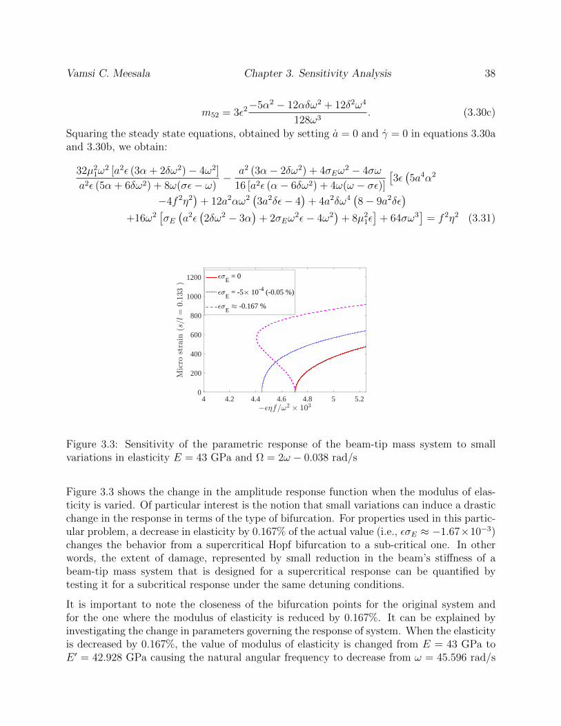
Vamsi C. Meesala Chapter 3. Sensitivity Analysis 38
m52 = 3ε2−5α2 − 12αδω2 + 12δ2ω4
128ω3. (3.30c)
Squaring the steady state equations, obtained by setting a = 0 and γ = 0 in equations 3.30aand 3.30b, we obtain:
32µ21ω
2 [a2ε (3α + 2δω2)− 4ω2]
a2ε (5α + 6δω2) + 8ω(σε− ω)− a2 (3α− 2δω2) + 4σEω
2 − 4σω
16 [a2ε (α− 6δω2) + 4ω(ω − σε)][3ε(5a4α2
−4f 2η2)
+ 12a2αω2(3a2δε− 4
)+ 4a2δω4
(8− 9a2δε
)+16ω2
[σE(a2ε(2δω2 − 3α
)+ 2σEω
2ε− 4ω2)
+ 8µ21ε]
+ 64σω3]
= f 2η2 (3.31)
4 4.2 4.4 4.6 4.8 5 5.20
200
400
600
800
1000
1200 E = 0
E = -5 10-4 (-0.05 %)
E -0.167 %
Figure 3.3: Sensitivity of the parametric response of the beam-tip mass system to smallvariations in elasticity E = 43 GPa and Ω = 2ω − 0.038 rad/s
Figure 3.3 shows the change in the amplitude response function when the modulus of elas-ticity is varied. Of particular interest is the notion that small variations can induce a drasticchange in the response in terms of the type of bifurcation. For properties used in this partic-ular problem, a decrease in elasticity by 0.167% of the actual value (i.e., εσE ≈ −1.67×10⁻³)changes the behavior from a supercritical Hopf bifurcation to a sub-critical one. In otherwords, the extent of damage, represented by small reduction in the beam’s stiffness of abeam-tip mass system that is designed for a supercritical response can be quantified bytesting it for a subcritical response under the same detuning conditions.
It is important to note the closeness of the bifurcation points for the original system andfor the one where the modulus of elasticity is reduced by 0.167%. It can be explained byinvestigating the change in parameters governing the response of system. When the elasticityis decreased by 0.167%, the value of modulus of elasticity is changed from E = 43 GPa toE ′ = 42.928 GPa causing the natural angular frequency to decrease from ω = 45.596 rad/s
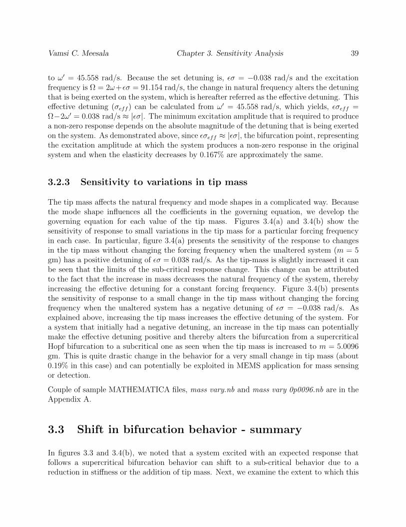
Vamsi C. Meesala Chapter 3. Sensitivity Analysis 39
to ω′ = 45.558 rad/s. Because the set detuning is, εσ = −0.038 rad/s and the excitationfrequency is Ω = 2ω+εσ = 91.154 rad/s, the change in natural frequency alters the detuningthat is being exerted on the system, which is hereafter referred as the effective detuning. Thiseffective detuning (σeff ) can be calculated from ω′ = 45.558 rad/s, which yields, εσeff =Ω−2ω′ = 0.038 rad/s ≈ |εσ|. The minimum excitation amplitude that is required to producea non-zero response depends on the absolute magnitude of the detuning that is being exertedon the system. As demonstrated above, since εσeff ≈ |εσ|, the bifurcation point, representingthe excitation amplitude at which the system produces a non-zero response in the originalsystem and when the elasticity decreases by 0.167% are approximately the same.
3.2.3 Sensitivity to variations in tip mass
The tip mass affects the natural frequency and mode shapes in a complicated way. Becausethe mode shape influences all the coefficients in the governing equation, we develop thegoverning equation for each value of the tip mass. Figures 3.4(a) and 3.4(b) show thesensitivity of response to small variations in the tip mass for a particular forcing frequencyin each case. In particular, figure 3.4(a) presents the sensitivity of the response to changesin the tip mass without changing the forcing frequency when the unaltered system (m = 5gm) has a positive detuning of εσ = 0.038 rad/s. As the tip-mass is slightly increased it canbe seen that the limits of the sub-critical response change. This change can be attributedto the fact that the increase in mass decreases the natural frequency of the system, therebyincreasing the effective detuning for a constant forcing frequency. Figure 3.4(b) presentsthe sensitivity of response to a small change in the tip mass without changing the forcingfrequency when the unaltered system has a negative detuning of εσ = −0.038 rad/s. Asexplained above, increasing the tip mass increases the effective detuning of the system. Fora system that initially had a negative detuning, an increase in the tip mass can potentiallymake the effective detuning positive and thereby alters the bifurcation from a supercriticalHopf bifurcation to a subcritical one as seen when the tip mass is increased to m = 5.0096gm. This is quite drastic change in the behavior for a very small change in tip mass (about0.19% in this case) and can potentially be exploited in MEMS application for mass sensingor detection.
Couple of sample MATHEMATICA files, mass vary.nb and mass vary 0p0096.nb are in theAppendix A.
3.3 Shift in bifurcation behavior - summary
In figures 3.3 and 3.4(b), we noted that a system excited with an expected response thatfollows a supercritical bifurcation behavior can shift to a sub-critical behavior due to areduction in stiffness or the addition of tip mass. Next, we examine the extent to which this
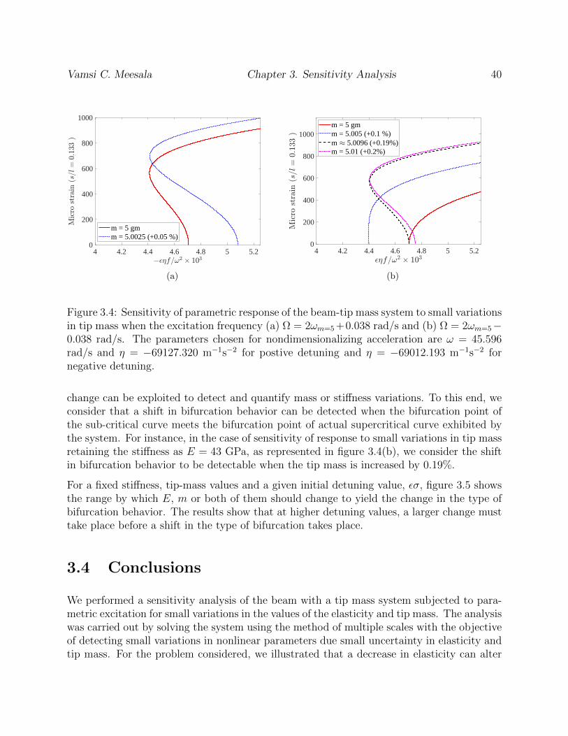
Vamsi C. Meesala Chapter 3. Sensitivity Analysis 40
4 4.2 4.4 4.6 4.8 5 5.20
200
400
600
800
1000
m = 5 gmm = 5.0025 (+0.05 %)
(a)
4 4.2 4.4 4.6 4.8 5 5.20
200
400
600
800
1000m = 5 gmm = 5.005 (+0.1 %)m 5.0096 (+0.19%)m = 5.01 (+0.2%)
(b)
Figure 3.4: Sensitivity of parametric response of the beam-tip mass system to small variationsin tip mass when the excitation frequency (a) Ω = 2ωm=5 +0.038 rad/s and (b) Ω = 2ωm=5−0.038 rad/s. The parameters chosen for nondimensionalizing acceleration are ω = 45.596rad/s and η = −69127.320 m−1s−2 for postive detuning and η = −69012.193 m−1s−2 fornegative detuning.
change can be exploited to detect and quantify mass or stiffness variations. To this end, weconsider that a shift in bifurcation behavior can be detected when the bifurcation point ofthe sub-critical curve meets the bifurcation point of actual supercritical curve exhibited bythe system. For instance, in the case of sensitivity of response to small variations in tip massretaining the stiffness as E = 43 GPa, as represented in figure 3.4(b), we consider the shiftin bifurcation behavior to be detectable when the tip mass is increased by 0.19%.
For a fixed stiffness, tip-mass values and a given initial detuning value, εσ, figure 3.5 showsthe range by which E, m or both of them should change to yield the change in the type ofbifurcation behavior. The results show that at higher detuning values, a larger change musttake place before a shift in the type of bifurcation takes place.
3.4 Conclusions
We performed a sensitivity analysis of the beam with a tip mass system subjected to para-metric excitation for small variations in the values of the elasticity and tip mass. The analysiswas carried out by solving the system using the method of multiple scales with the objectiveof detecting small variations in nonlinear parameters due small uncertainty in elasticity andtip mass. For the problem considered, we illustrated that a decrease in elasticity can alter
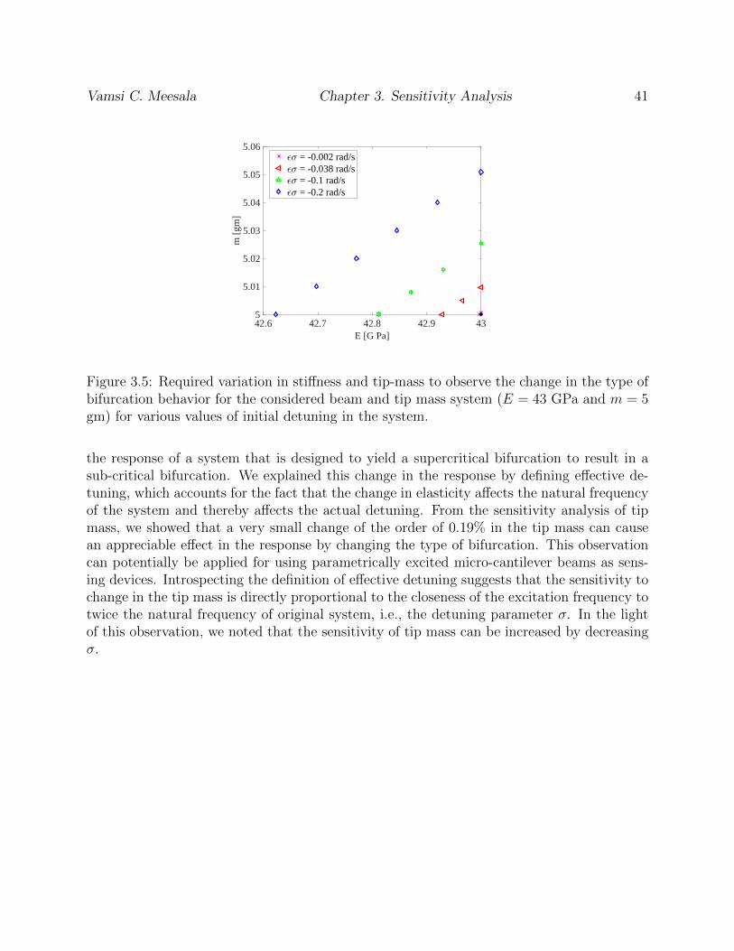
Vamsi C. Meesala Chapter 3. Sensitivity Analysis 41
42.6 42.7 42.8 42.9 43E [G Pa]
5
5.01
5.02
5.03
5.04
5.05
5.06
m [
gm]
= -0.002 rad/s = -0.038 rad/s = -0.1 rad/s = -0.2 rad/s
Figure 3.5: Required variation in stiffness and tip-mass to observe the change in the type ofbifurcation behavior for the considered beam and tip mass system (E = 43 GPa and m = 5gm) for various values of initial detuning in the system.
the response of a system that is designed to yield a supercritical bifurcation to result in asub-critical bifurcation. We explained this change in the response by defining effective de-tuning, which accounts for the fact that the change in elasticity affects the natural frequencyof the system and thereby affects the actual detuning. From the sensitivity analysis of tipmass, we showed that a very small change of the order of 0.19% in the tip mass can causean appreciable effect in the response by changing the type of bifurcation. This observationcan potentially be applied for using parametrically excited micro-cantilever beams as sens-ing devices. Introspecting the definition of effective detuning suggests that the sensitivity tochange in the tip mass is directly proportional to the closeness of the excitation frequency totwice the natural frequency of original system, i.e., the detuning parameter σ. In the lightof this observation, we noted that the sensitivity of tip mass can be increased by decreasingσ.
Chapter 4
Identification of nonlinearpiezoelectric coefficients
Attention to piezoelectric materials has increased dramatically in recent years. This interestrises from their potential for their use in many applications for various objectives. Theyhave been suggested for developing self powered micro systems and sensors [53–58], active-passive vibration control and damping systems [59–64], broadband energy harvesters [65–68]and impedance based structural health monitoring devices [57, 69, 70]. In more recent stud-ies, piezoelectric/ceramic materials have been proposed in biomedical applications as loadand wear sensors for knee joints [71, 72] and as receivers to oxygenate tumors and chargepacemakers [73–75]. To augment the power generated, specific designs have been proposedthat produce large strains and thereby generating more power [76–78]. Extending the realmof applications of piezoelectric materials comes with a price, as large strains can cause thematerial to behave in a nonlinear manner and exhibit amplitude-dependent resonant fre-quencies, super-harmonics in the response, saturation and hysteresis behaviors. As such,identification of the nonlinear electromechanical constitutive relation must be performed todesign, analyze, optimize and/or exploit such behaviors.
Aurelle et al. [32] and Guyomar et al. [33] presented a nonlinear electromechanical consti-tutive relation to study the saturation and hysteresis behavior that they observed in theirexperiments on ultrasonic transducers. Wagner and Hagedorn [34] derived an equation forthe electric enthalpy density that accounts for nonlinearities in piezoelectric response. Theydemonstrated that a bi-morph cannot be used to study the quadratic nonlinearities becausethe symmetrical nature of the bi-morph eliminates the effects of quadratic nonlinearities. Areview of the nonlinear behavior of piezoelectric materials was presented by Leadenham andErturk [79]. We note that the most common approach employed to estimate the parame-ters governing the nonlinear behavior in the above mentioned references has consisted of anoptimized curve fitting procedure and, postulate that there is a need to develop a holisticparameter identification scheme that utilizes the vibration behavior.
42
Vamsi C. Meesala Chapter 4. Parameter identification 43
Analyzing the vibration behavior is probably the most insightful and physical way for pa-rameter identification. Free vibration tests are commonly used for estimating damping ratioof a structure and in piezoelectric energy harvesters. The frequency response functions ofdisplacement and voltage generated are used to identify characteristic capacitance and elec-tromechanical coupling of the harvester. Nayfeh [80] presented a parameter identificationprocedure for a generic nonlinear coupled oscillator that exploits the hysteresis and sub crit-ical bufurcation exhibited by a generic oscillator. Zavodney [81] generalized the theory toidentify and estimate the nonlinearity in the system from random excitations and forcingand frequency sweeps. Hajj et al. [82] combined perturbation techniques and bispectralanalysis to characterize nonlinear damping from experimental data of three beam and twomass system. A concise review of nonlinear system identification in structural dynamics ispresented by Kerschen et al. [83]. To date, the parameter identification work for smart andintelligent systems has concentrated on micro resonators, where the system is representedas a Duffing oscillator with geometric nonlinearity [84, 85] without a specific approach toidentify nonlinear piezoelectric coefficients.
In this paper, we consider an unsymmetrical piezoelectric energy harvester and propose aparameter identification scheme to identify nonlinear piezoelectric coefficients by exploitingthe principal mode resonant response. We consider a beam with tip mass and a singlepiezoelectric layer subjected to direct excitation as an unsymmetrical piezoelectric energyharvester and first derive the governing equations of the first mode using the electric enthalpydensity representation introduced by Wagner and Hagedorn [34]. We then use the method ofmultiple scales [46, 50] to determine the approximate solution of the response to a principalmode resonant excitation and under open circuit conditions (i.e., high load resistance). Weargue that the characteristic nonlinear response of the harvester predicted by the method ofmultiple scales as approximate solution and steady state amplitude response relations canbe used for estimating nonlinear parameters and propose a holistic parameter identificationscheme. By choosing a numerical example, we validate the proposed parameter identificationscheme and estimate the material parameters governing the nonlinear behavior.
4.1 Mathematical Modeling
A cantilever beam system with a tip mass m, partially covered with piezoelectric layer,subjected to direct excitation is considered for the analysis as shown in the figure 2.1. Thebeam with length l, width bp, thickness hs and mass per unit length ρs is bonded with apiezoelectric layer of length l1, width b, thickness hp and mass per unit length ρp that isconnected to a load resistance, R. To derive the governing equation and energy harvested,we employ the generalized Hamilton principle for electronic transducers [34,86–89], which iswritten as: ∫ t2
t1
(δT − δ∆ + δWnc) dt = 0 (4.1)
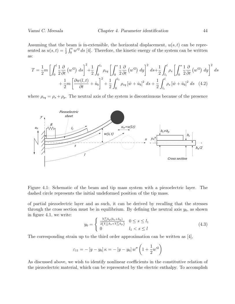
Vamsi C. Meesala Chapter 4. Parameter identification 44
Assuming that the beam is in-extensible, the horizontal displacement, u(s, t) can be repre-sented as u(s, t) = 1
2
∫ s0w′2 ds [4]. Therefore, the kinetic energy of the system can be written
as:
T =1
2m
[∫ l
0
1
2
∂
∂t
(w′2)ds
]2
+1
2
∫ l1
0
ρeq
[∫ s
0
1
2
∂
∂t
(w′2)dy
]2
ds+1
2
∫ l
l1
ρs
[∫ s
0
1
2
∂
∂t
(w′2)dy
]2
ds
+1
2m
[∂w(l, t)
∂t+ ub
]2
+1
2
∫ l1
0
ρeq [w + ub]2 ds+
1
2
∫ l
l1
ρs [w + ub]2 ds (4.2)
where ρeq = ρs + ρp. The neutral axis of the system is discontinuous because of the presence
Cross section
hs+hp
hs
y
y0x
ub
Piezoelectric sheet
s
l
l1
R
w(s, t)
um=u(l,t)
hs/2
Figure 4.1: Schematic of the beam and tip mass system with a piezoelectric layer. Thedashed circle represents the initial undeformed position of the tip mass.
of partial piezoelectric layer and as such, it can be derived by recalling that the stressesthrough the cross section must be in equilibrium. By defining the neutral axis y0, as shownin figure 4.1, we write:
y0 =
Y p11hp(hs+hp)
2(Y s11hs+Y p
11hp)0 ≤ s ≤ l1
0 l1 < s ≤ l(4.3)
The corresponding strain up to the third order approximation can be written as [4],
ε11 = − [y − y0]κ = − [y − y0]w′′(
1 +1
2w′2)
As discussed above, we wish to identify nonlinear coefficients in the constitutive relation ofthe piezoelectric material, which can be represented by the electric enthalpy. To accomplish
Vamsi C. Meesala Chapter 4. Parameter identification 45
this, we account for the potential energy and use the electric enthalpy derived by Wagnerand Hagedorn [34] and write
∆ =
∫ (1
2Y s
11ε211 +
1
2Y p
11ε211 − e31ε11E3 −
1
2α3E3ε
211 −
1
2εS33E
23 +
1
6α1ε
311 −
1
6α2ε
311E3 +
1
8α4ε
411
)dv
(4.4)where Y s
11, Y p11, e31 and εS33 are respectively the Young’s modulus of elasticity of the beam
(substrate), Young’s modulus of piezoelectric material, piezoelectric coupling co-efficient anddielectric (or piezoelectric permittivity) constant. E3 is the induced electric field and is givenby
E3 =
−VH
hphs2≤ y ≤ hs
2+ hp
0 −hs2≤ y < hs
2
(4.5)
where VH(s, t) = V (t) [H(s)−H(s− l1)] = V (t)Hf(s), VH(s, t)n = V (t)n [H(s)−H(s− l1)] =V (t)nHf(s) and H(x) is Heaviside step function.
The electric enthalpy in equation 4.4 can be re-written as:
∆ =1
2
∫ l1
0
Y Ieqw′′2 [1 + w′2
]ds−
∫ l1
0
e31Λ1w′′(1 +
1
2w′2)
VHhp
ds+1
2
∫ l1
0
α3Ipw′′2VHhp
ds
− 1
2
∫ l1
0
εS33
V 2Hb
hpds− 1
6
∫ l1
0
α1Λ2w′′3 ds− 1
6
∫ l1
0
α2VHhp
Λ2w′′3 ds
+1
8
∫ l1
0
α4Λ3w′′4 ds+
1
2
∫ l
l1
Y s11Isw
′′2 [1 + w′2]ds (4.6)
where Y Ieq = (Y I)s + Y p11Ip,
(Y I)s =
∫ hs2
−hs2
Y s11b (y − y0)2 dy = Y s
11
b
3
[(hs2− y0
)3
+
(hs2
+ y0
)3], (4.7a)
Ip =
∫ hs2
+hp
hs2
bp (y − y0)2 dy =bp3
[(hs2
+ hp − y0
)3
−(hs2− y0
)3], (4.7b)
Λ1 =bp2
[(hs2
+ hp − y0
)2
−(hs2− y0
)2], Λ2 =
bp4
[(hs2
+ hp − y0
)4
−(hs2− y0
)4],
(4.7c)
Λ3 =bp5
[(hs2
+ hp − y0
)5
−(hs2− y0
)5], and Is =
b
12h3s. (4.7d)
The virtual work done by the non conservative forces is represented by
δWnc = −∫ l
0
c1w(0,1)(s, t)δw(s, t) ds (4.8)
Vamsi C. Meesala Chapter 4. Parameter identification 46
where c1 is structural damping coefficient. Substituting equations 4.2, 4.6, and 4.8 intoequation 4.1, we obtain the piece-wise distributed parameter governing equation of motionsas
− ρeqw − c1w − Y Ieq(w′′′′ + [w′(w′w′′)′]′)− ρeq2
[w′∫ s
l1
∫ θ
0
∂2
∂t2(w′2)dy dθ
]′+mw′′
2
∫ l
0
∂2
∂t2(w′2)ds+ e31IIp
[w′2V Hf ′′
2hp+w′′w′V Hf ′
hp+V Hf ′′
hp
]+ α2Λ2
[V Hf ′′w′′2
2hp+
2w′′w′′′V Hf ′
hp+w′′′2V Hf
hp+w′′′′w′′V Hf
hp
]+ α1Λ2
[w′′′2 + w′′w′′′′
]− α3Ip
[V Hf ′′w′′
hp+
2V hf ′w′′′
hp+V Hfw′′′′
hp
]+ α4Λ3
[−3w′′w′′′2 − 3
2w′′2w′′′′
]+ρs2w′′∫ l
l1
∫ θ
0
∂2
∂t2(w′2)dy dθ − ρequb = 0 (4.9)
for 0 < s < l1,
− ρsw − c1w − Y s11Is(w
′′′′ + [w′(w′w′′)′]′)
− ρs2
[w′∫ s
l
∫ θ
0
∂2
∂t2(w′2)dy dθ
]′+mw′′
2
∫ l
11
∂2
∂t2(w′2)ds− ρsub = 0 (4.10)
for l1 < s < l, and the corresponding electrical equation is
e31Λ1
[∫ l1
0
w′′
hpds+
∫ l
0
w′2w′′
2hpds
]+ α2Λ2
∫ l1
0
w′′3
6hpds
+
∫ l1
0
ε33V b
hpds− α3Ip
∫ l1
0
w′′2
2hpds = Q(t) (4.11)
Since the beam is clamped at s = 0, the essential boundary conditions at s = 0 are given by
w(0, t) = 0 w(1,0)(0, t) = 0 (4.12)
and the natural nonlinear boundary conditions at s = l, which are moment and shear forcebalance equations, obtained from the generalized Hamilton principle are written as
Y s11Is
(w′′w′2 + w′′
)∣∣s=l
= 0 =⇒ w′′(l, t) = 0 (4.13)
− mub + Y s11Is
(w′′′w′2 + w′′2w′ + w′′′
)−mw′
∫ l
0
∂2
∂t2
(w′2
2
)ds−mw
∣∣∣∣s=l
= 0 (4.14)
Vamsi C. Meesala Chapter 4. Parameter identification 47
The generalized Hamilton’s principle also yields us the moment and shear force balanceequations at s = l1, which serve as the compatibility conditions at s = l1 and are written as
e31Λ1
[w′2V Hf
2hp+V Hf
hp
]+
1
2α1Λ2w
′′2 +1
2hpα2Λ2HfV w
′′2 − 1
2α4Λ3w
′′3
−α3Ipw′′V Hf
hp− Y Ieq
(w′′w′2 + w′′
)+ Y s
11Is(w′′w′2 + w′′
)∣∣∣∣s=l1
= 0 (4.15)
−e31Λ1
(w′2V Hf ′
2hp+V Hf ′
hp
)+ Y Ieq
(w′′′w′2 + w′′2w′ + w′′′
)− Y s
11Is(w′′′w′2 + w′′2w′ + w′′′
)−α2Λ2
(w′′2V Hf ′
2hp+V Hfw′′w′′′
hp
)− α1Λ2w
′′w′′′ +α3Ip
(w′′V Hf ′
hp+w′′′V Hf
hp
)+
3
2α4Λ3w
′′2w′′′∣∣∣∣s=l1
= 0 (4.16)
4.1.1 Reduced order model - Galerkin discretization
To simplify the representative model and to study the response to a principal mode resonanceexcitation, we employ a Galerkin discretization and perform weighted residual method todetermine the governing equation of the first mode. To this end, we determine the linearmode shapes of the system by considering the undamped, unforced, short circuited [V (t) = 0]and linear free vibration description of motion as
ρeqw + Y Ieqw′′′′ = 0 0 < s < l1
ρsw + Y s11Isw
′′′′ = 0 l1 < s < l(4.17)
Assuming the discretization as
w(s, t) =
∑Mi=1 φi(s)qi(t) 0 < s < l1∑Mi=1 ψi(s)qi(t) l1 < s < l
(4.18)
and substituting into equation 4.17, while realizing that q = −ω2nq, where ωn is the natural
frequency of the nth-mode, we obtain
φi′′′′ = λ1iφi 0 < s < l1 (4.19a)
ψi′′′′ = λ4
2iψi l1 < s < l (4.19b)
whose general solution is of the form
φi(s) = A1 cos(λ1is) +B1 sin(λ1is) + C1 cosh(λ1is) +D1 sinh(λ1is) 0 < s < l1 (4.20a)
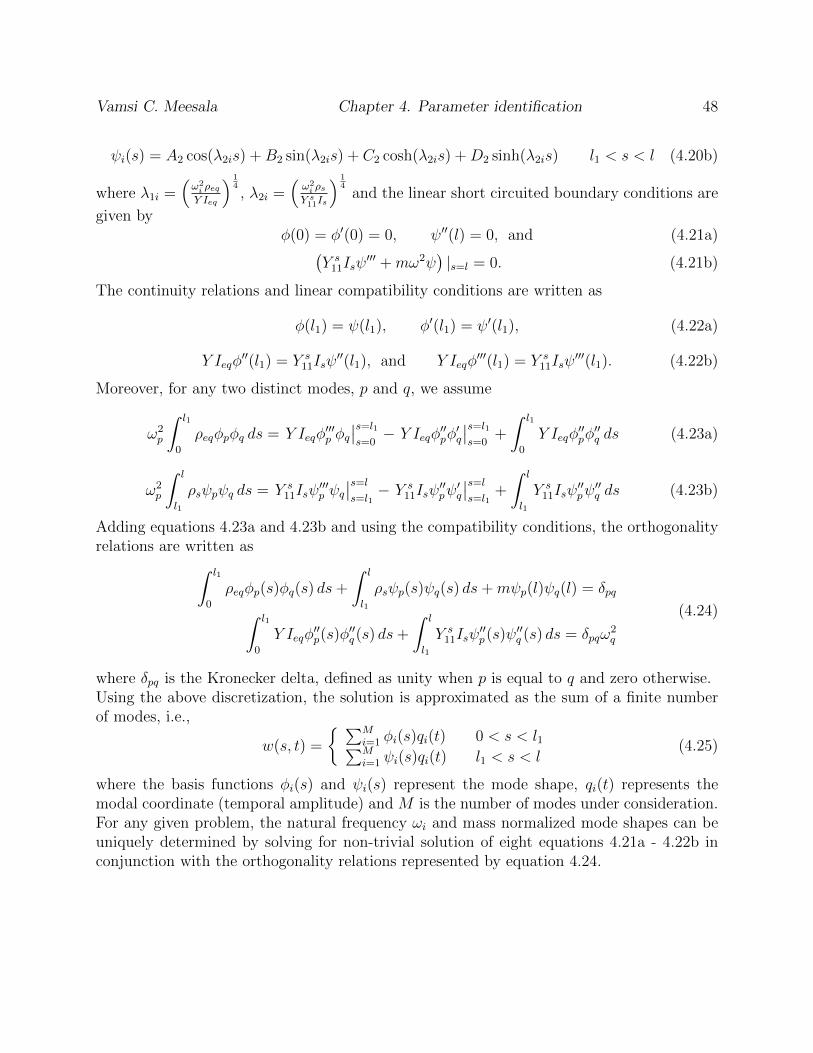
Vamsi C. Meesala Chapter 4. Parameter identification 48
ψi(s) = A2 cos(λ2is) +B2 sin(λ2is) + C2 cosh(λ2is) +D2 sinh(λ2is) l1 < s < l (4.20b)
where λ1i =(ω2i ρeqY Ieq
) 14, λ2i =
(ω2i ρs
Y s11Is
) 14
and the linear short circuited boundary conditions are
given byφ(0) = φ′(0) = 0, ψ′′(l) = 0, and (4.21a)(
Y s11Isψ
′′′ +mω2ψ)|s=l = 0. (4.21b)
The continuity relations and linear compatibility conditions are written as
φ(l1) = ψ(l1), φ′(l1) = ψ′(l1), (4.22a)
Y Ieqφ′′(l1) = Y s
11Isψ′′(l1), and Y Ieqφ
′′′(l1) = Y s11Isψ
′′′(l1). (4.22b)
Moreover, for any two distinct modes, p and q, we assume
ω2p
∫ l1
0
ρeqφpφq ds = Y Ieqφ′′′p φq∣∣s=l1s=0− Y Ieqφ
′′pφ′q
∣∣s=l1s=0
+
∫ l1
0
Y Ieqφ′′pφ′′q ds (4.23a)
ω2p
∫ l
l1
ρsψpψq ds = Y s11Isψ
′′′p ψq
∣∣s=ls=l1− Y s
11Isψ′′pψ′q
∣∣s=ls=l1
+
∫ l
l1
Y s11Isψ
′′pψ′′q ds (4.23b)
Adding equations 4.23a and 4.23b and using the compatibility conditions, the orthogonalityrelations are written as∫ l1
0
ρeqφp(s)φq(s) ds+
∫ l
l1
ρsψp(s)ψq(s) ds+mψp(l)ψq(l) = δpq∫ l1
0
Y Ieqφ′′p(s)φ
′′q(s) ds+
∫ l
l1
Y s11Isψ
′′p(s)ψ′′q (s) ds = δpqω
2q
(4.24)
where δpq is the Kronecker delta, defined as unity when p is equal to q and zero otherwise.Using the above discretization, the solution is approximated as the sum of a finite numberof modes, i.e.,
w(s, t) =
∑Mi=1 φi(s)qi(t) 0 < s < l1∑Mi=1 ψi(s)qi(t) l1 < s < l
(4.25)
where the basis functions φi(s) and ψi(s) represent the mode shape, qi(t) represents themodal coordinate (temporal amplitude) and M is the number of modes under consideration.For any given problem, the natural frequency ωi and mass normalized mode shapes can beuniquely determined by solving for non-trivial solution of eight equations 4.21a - 4.22b inconjunction with the orthogonality relations represented by equation 4.24.
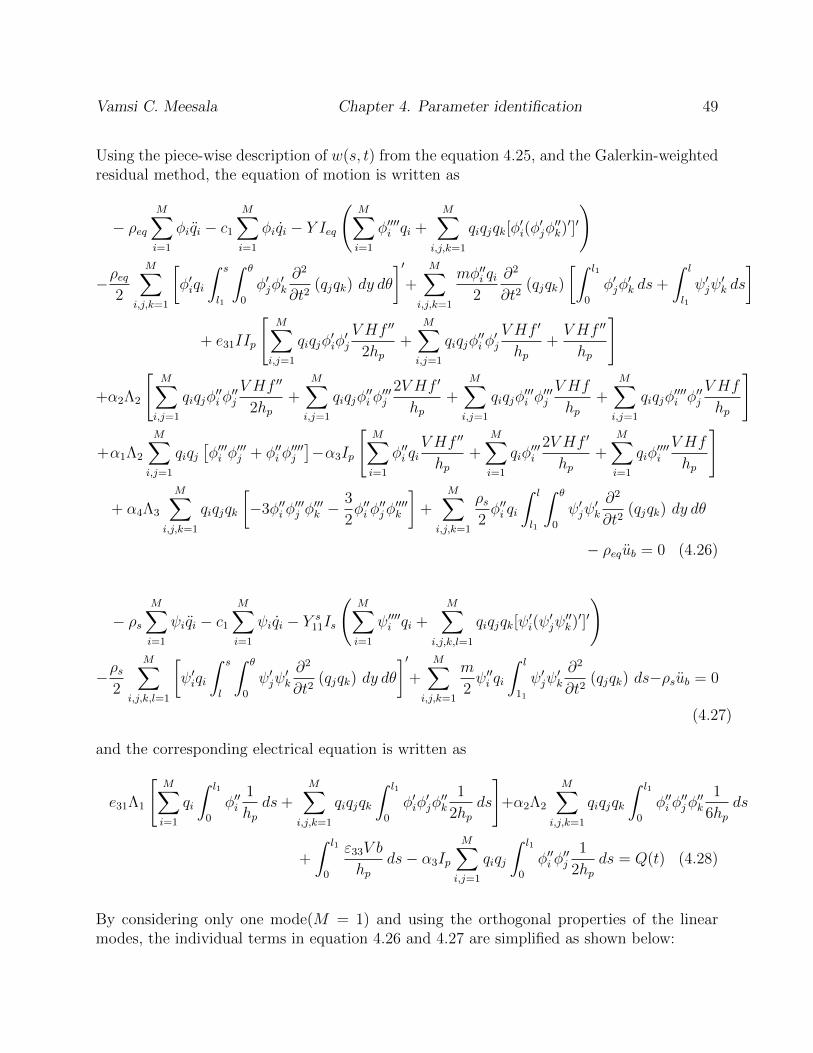
Vamsi C. Meesala Chapter 4. Parameter identification 49
Using the piece-wise description of w(s, t) from the equation 4.25, and the Galerkin-weightedresidual method, the equation of motion is written as
− ρeqM∑i=1
φiqi − c1
M∑i=1
φiqi − Y Ieq
(M∑i=1
φ′′′′i qi +M∑
i,j,k=1
qiqjqk[φ′i(φ′jφ′′k)′]′
)
−ρeq2
M∑i,j,k=1
[φ′iqi
∫ s
l1
∫ θ
0
φ′jφ′k
∂2
∂t2(qjqk) dy dθ
]′+
M∑i,j,k=1
mφ′′i qi2
∂2
∂t2(qjqk)
[∫ l1
0
φ′jφ′k ds+
∫ l
l1
ψ′jψ′k ds
]
+ e31IIp
[M∑i,j=1
qiqjφ′iφ′j
V Hf ′′
2hp+
M∑i,j=1
qiqjφ′′i φ′j
V Hf ′
hp+V Hf ′′
hp
]
+α2Λ2
[M∑i,j=1
qiqjφ′′i φ′′j
V Hf ′′
2hp+
M∑i,j=1
qiqjφ′′i φ′′′j
2V Hf ′
hp+
M∑i,j=1
qiqjφ′′′i φ′′′j
V Hf
hp+
M∑i,j=1
qiqjφ′′′′i φ′′j
V Hf
hp
]
+α1Λ2
M∑i,j=1
qiqj[φ′′′i φ
′′′j + φ′′i φ
′′′′j
]−α3Ip
[M∑i=1
φ′′i qiV Hf ′′
hp+
M∑i=1
qiφ′′′i
2V Hf ′
hp+
M∑i=1
qiφ′′′′i
V Hf
hp
]
+ α4Λ3
M∑i,j,k=1
qiqjqk
[−3φ′′i φ
′′′j φ′′′k −
3
2φ′′i φ
′′jφ′′′′k
]+
M∑i,j,k=1
ρs2φ′′i qi
∫ l
l1
∫ θ
0
ψ′jψ′k
∂2
∂t2(qjqk) dy dθ
− ρequb = 0 (4.26)
− ρsM∑i=1
ψiqi − c1
M∑i=1
ψiqi − Y s11Is
(M∑i=1
ψ′′′′i qi +M∑
i,j,k,l=1
qiqjqk[ψ′i(ψ′jψ′′k)′]′
)
−ρs2
M∑i,j,k,l=1
[ψ′iqi
∫ s
l
∫ θ
0
ψ′jψ′k
∂2
∂t2(qjqk) dy dθ
]′+
M∑i,j,k=1
m
2ψ′′i qi
∫ l
11
ψ′jψ′k
∂2
∂t2(qjqk) ds−ρsub = 0
(4.27)
and the corresponding electrical equation is written as
e31Λ1
[M∑i=1
qi
∫ l1
0
φ′′i1
hpds+
M∑i,j,k=1
qiqjqk
∫ l1
0
φ′iφ′jφ′′k
1
2hpds
]+α2Λ2
M∑i,j,k=1
qiqjqk
∫ l1
0
φ′′i φ′′jφ′′k
1
6hpds
+
∫ l1
0
ε33V b
hpds− α3Ip
M∑i,j=1
qiqj
∫ l1
0
φ′′i φ′′j
1
2hpds = Q(t) (4.28)
By considering only one mode(M = 1) and using the orthogonal properties of the linearmodes, the individual terms in equation 4.26 and 4.27 are simplified as shown below:

Vamsi C. Meesala Chapter 4. Parameter identification 50
Y Ieqq1
∫ l1
0
φ1φ′′′′1 dx = Y Ieqq1
∫ l1
0
φ′′1φ′′1 ds+ Y Ieqq1φ
′′′1 (l1)φ1(l1)− Y Ieqq1φ
′′1(l1)φ′1(l1) (4.29)
Y Ieqq31
∫ l1
0
φ1(φ′1(φ′1φ′′1)′)′ ds = (Y Ieqq
31φ1φ
′21 φ′′′1 + Y Ieqq
31φ1φ
′1φ′′21 )|s=l1
− (Y Ieqq31φ′31 φ′′1)|s=l1 + 2Y Ieqq
31
∫ l1
0
φ′21 φ′′21 ds (4.30)
ρeqq1(q21+q1q1)
∫ l1
0
φ1
(φ′1
∫ s
l1
∫ θ
0
φ′21 dy dθ
)′ds = −ρeqq1(q2
1+q1q1)
∫ l1
0
φ′21
(∫ s
l1
∫ θ
0
φ′21 dy dθ
)ds
(4.31)
−mq1(q1q1 + q21)
∫ l1
0
φ1φ′′1
(∫ l1
0
φ′21 dy +
∫ l
l1
ψ′21 dy
)ds =
mq1(q1q1 + q21)
[− (φ′1φ1)|s=l1
∫ l
l1
ψ′21 ds+
∫ l1
0
φ′21 ds
∫ l
l1
ψ′21 ds
]+mq1(q1q1 + q2
1)
[−(φ′1φ1
∫ l1
0
φ′21 ds
)∣∣∣∣s=l1
+
(∫ l1
0
φ′21 ds
)2]
(4.32)
−e31IIpq21
V
2hp
∫ l1
0
φ1φ′21 Hf
′′ ds = −e31Λ1q21
V
2hpφ′21 φ1Hf
′ |s=l1+e31Λ1q21
V
hp
∫ l1
0
φ1φ′1φ′′1Hf
′ ds
+ e31Λ1q21
V
2hp
∫ l1
0
φ′31 Hf′ ds
= −e31Λ1q21
V
2hpφ′21 φ1Hf
′ |s=l1 + e31Λ1q21
V
hp
∫ l1
0
φ1φ′1φ′′1Hf
′ ds
+ e31Λ1q21
V
2hpφ′31 Hf |s=l1 − e31Λ1q
21
3V
2hp
∫ l1
0
φ′21 φ′′1Hf ds (4.33)
−e31Λ1V
hp
∫ l1
0
φ1Hf′′ ds = − e31Λ1
V
hpφ1Hf
′∣∣∣∣s=l1
+e31Λ1V
hpφ′1Hf.
∣∣∣∣s=l1
−e31Λ1V
hp
∫ l1
0
φ′′1Hf ds
(4.34)

Vamsi C. Meesala Chapter 4. Parameter identification 51
−α2Λ2q21
V
2hp
∫ l1
0
φ1φ′′1
2Hf ′′ ds = −α2Λ2q21
V
2hpφ1φ
′′1
2Hf ′|s=l1+α2Λ2q21
V
hp
∫ l1
0
φ1φ′′1φ′′′1 Hf
′ ds
+ α2Λ2q21
V
2hpφ′1φ
′′1
2Hf
∣∣∣∣s=l1
− α2Λ2q21
V
2hp
∫ l1
0
(φ′′′1
3 + 2φ′1φ′′1φ′′′1
)Hf ds (4.35)
− α2Λ2q21
V
hp
∫ l1
0
φ1φ′′1φ′′′1 Hf
′ ds = −α2Λ2q21
V
hpφ1φ
′′1φ′′′1 Hf
∣∣∣∣s=l1
+ α2Λ2q21
V
hp
∫ l1
0
(φ′1φ
′′1φ′′′1 + φ1φ
′′′1
2 + φ1φ′′1φ′′′′1
)Hf ds (4.36)
− α1Λ2q21
∫ l1
0
φ1φ′′1φ′′′′1 ds = − α1Λ2q
21φ1φ
′′1φ′′′1
∣∣s=l1
+ α1Λ2q21
∫ l1
0
φ1φ′′′1
2 ds
+ α1Λ2q21φ′1φ′′1φ′′1
∣∣s=l1− α1Λ2q
21
∫ l1
0
(φ′′1
2 + φ′1φ′′′1
)φ′′1 ds
since,−α1Λ2q21
∫ l1
0
φ′1φ′′1φ′′′1 ds = −1
2α1Λ2q
21φ′1φ′′1
2|s=l1 +1
2α1Λ2q
21
∫ l1
0
φ′′13 ds
− α1Λ2q21
∫ l1
0
φ1φ′′1φ′′′′1 ds = − α1Λ2q
21φ1φ
′′1φ′′′1
∣∣s=l1
+ α1Λ2q21
∫ l1
0
φ1φ′′′1
2 ds
+ α1Λ2q21φ′1φ′′1φ′′1
∣∣s=l1− 1
2α1Λ2q
21φ′1φ′′1
2|s=l1 −1
2α1Λ2q
21
∫ l1
0
φ′′13 ds (4.37)
α3IpV
hpq1
∫ l1
0
φ1 (φ′′1Hf′′ + φ′′′′1 Hf + 2Hf ′φ′′′1 ) ds = − α3Ip
V
hpq1Hfφ
′1φ′′1
∣∣∣∣s=l1
+ α3IpV
hpq1 (Hf ′φ1φ
′′1 +Hfφ1φ
′′′1 )
∣∣∣∣s=l1
+ α3IpV
hpq1
∫ l1
0
Hfφ′′12 ds (4.38)
α4Λ3q31
∫ l1
0
(3φ1φ
′′1φ′′′21 +
3
2φ1φ
′′1
2φ′′′′1
)ds =
3
2α4Λ3q
31φ1φ
′′1
2φ′′′1
∣∣∣∣s=l1
− 1
2α4Λ3q
31φ′1φ′′31
∣∣∣∣s=l1
+1
2α4Λ3q
31
∫ l1
0
φ′′41 ds (4.39)
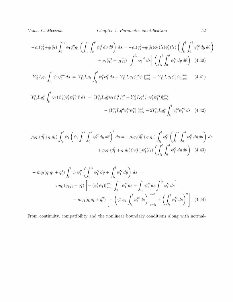
Vamsi C. Meesala Chapter 4. Parameter identification 52
−ρs(q21+q1q1)
∫ l1
0
φ1φ′′1q1
(∫ l
l1
∫ θ
0
ψ′21 dy dθ
)ds = −ρs(q2
1+q1q1)φ1(l1)φ′1(l1)
(∫ l
l1
∫ θ
0
ψ′21 dy dθ
)+ ρs(q
21 + q1q1)
[∫ l1
0
φ1′2 ds
](∫ l
l1
∫ θ
0
ψ′21 dy dθ
)(4.40)
Y s11Isq1
∫ l
l1
ψ1ψ′′′′1 ds = Y s
11Isq1
∫ l
l1
ψ′′1ψ′′1 ds+ Y s
11Isq1ψ′′′1 ψ1|s=ls=l1
− Y s11Isq1ψ
′′1ψ′1|s=ls=l1
(4.41)
Y s11Isq
31
∫ l
l1
ψ1(ψ′1(ψ′1ψ′′1)′)′ ds = (Y s
11Isq31ψ1ψ
′21 ψ′′′1 + Y s
11Isq31ψ1ψ
′1ψ′′21 )|s=ls=l1
− (Y s11Isq
31ψ′31 ψ′′1)|s=ls=l1
+ 2Y s11Isq
31
∫ l
l1
ψ′21 ψ′′21 ds (4.42)
ρsq1(q21+q1q1)
∫ l
l1
ψ1
(ψ′1
∫ s
l
∫ θ
0
ψ′21 dy dθ
)′ds = −ρsq1(q2
1+q1q1)
∫ l
l1
ψ′21
(∫ s
l
∫ θ
0
ψ′21 dy dθ
)ds
+ ρsq1(q21 + q1q1)ψ1(l1)ψ′1(l1)
(∫ l
l1
∫ θ
0
ψ′21 dy dθ
)(4.43)
−mq1(q1q1 + q21)
∫ l
l1
ψ1ψ′′1
(∫ l1
0
φ′21 dy +
∫ l
l1
ψ′21 dy
)ds =
mq1(q1q1 + q21)
[− (ψ′1ψ1)|s=ls=l1
∫ l1
0
φ′21 ds+
∫ l
l1
ψ′21 ds
∫ l1
0
φ′21 ds
]+mq1(q1q1 + q2
1)
[−(ψ′1ψ1
∫ l
l1
ψ′21 ds
)∣∣∣∣s=ls=l1
+
(∫ l
l1
ψ′21 ds
)2]
(4.44)
From continuity, compatibility and the nonlinear boundary conditions along with normal-
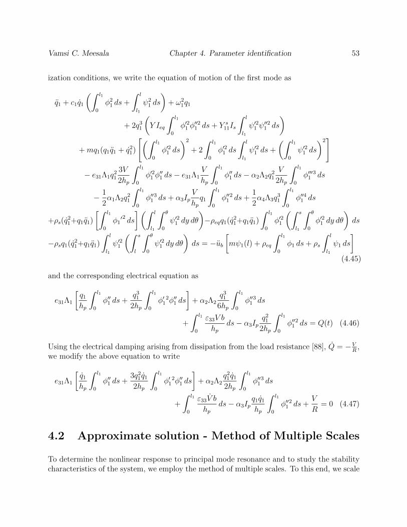
Vamsi C. Meesala Chapter 4. Parameter identification 53
ization conditions, we write the equation of motion of the first mode as
q1 + c1q1
(∫ l1
0
φ21 ds+
∫ l
l1
ψ21 ds
)+ ω2
1q1
+ 2q31
(Y Ieq
∫ l1
0
φ′21 φ′′21 ds+ Y s
11Is
∫ l
l1
ψ′21 ψ′′21 ds
)+mq1(q1q1 + q2
1)
[(∫ l1
0
φ′21 ds
)2
+ 2
∫ l1
0
φ′21 ds
∫ l
l1
ψ′21 ds+
(∫ l1
0
ψ′21 ds
)2]
− e31Λ1q21
3V
2hp
∫ l1
0
φ′21 φ′′1 ds− e31Λ1
V
hp
∫ l1
0
φ′′1 ds− α2Λ2q21
V
2hp
∫ l1
0
φ′′′13 ds
− 1
2α1Λ2q
21
∫ l1
0
φ′′13 ds+ α3Ip
V
hpq1
∫ l1
0
φ′′12 ds+
1
2α4Λ3q
31
∫ l1
0
φ′′41 ds
+ρs(q21+q1q1)
[∫ l1
0
φ1′2 ds
](∫ l
l1
∫ θ
0
ψ′21 dy dθ
)−ρeqq1(q2
1+q1q1)
∫ l1
0
φ′21
(∫ s
l1
∫ θ
0
φ′21 dy dθ
)ds
−ρsq1(q21+q1q1)
∫ l
l1
ψ′21
(∫ s
l
∫ θ
0
ψ′21 dy dθ
)ds = −ub
[mψ1(l) + ρeq
∫ l1
0
φ1 ds+ ρs
∫ l
l1
ψ1 ds
](4.45)
and the corresponding electrical equation as
e31Λ1
[q1
hp
∫ l1
0
φ′′1 ds+q3
1
2hp
∫ l1
0
φ′12φ′′1 ds
]+ α2Λ2
q31
6hp
∫ l1
0
φ′′13 ds
+
∫ l1
0
ε33V b
hpds− α3Ip
q21
2hp
∫ l1
0
φ′′12 ds = Q(t) (4.46)
Using the electrical damping arising from dissipation from the load resistance [88], Q = −VR
,we modify the above equation to write
e31Λ1
[q1
hp
∫ l1
0
φ′′1 ds+3q2
1 q1
2hp
∫ l1
0
φ′12φ′′1 ds
]+ α2Λ2
q21 q1
2hp
∫ l1
0
φ′′13 ds
+
∫ l1
0
ε33V b
hpds− α3Ip
q1q1
hp
∫ l1
0
φ′′12 ds+
V
R= 0 (4.47)
4.2 Approximate solution - Method of Multiple Scales
To determine the nonlinear response to principal mode resonance and to study the stabilitycharacteristics of the system, we employ the method of multiple scales. To this end, we scale
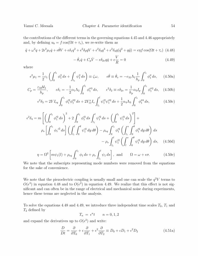
Vamsi C. Meesala Chapter 4. Parameter identification 54
the contributions of the different terms in the governing equations 4.45 and 4.46 appropriatelyand, by defining ub = f cos(Ωt+ τe), we re-write them as
q+ ω2q+ 2ε2µ1q+ εθV + εδ1q2 + ε2δ2qV + ε2δ3q
3 + ε2δ4q(q2 + qq) = εηf cos(Ωt+ τe) (4.48)
− θv q + CpV − εδ2vqq + εV
R= 0 (4.49)
where
ε2µ1 =1
2c1
(∫ l1
0
φ21 ds+
∫ l
l1
ψ21 ds
)≡ ζω, εθ ≡ θv = −e31Λ1
1
hp
∫ l1
0
φ′′1 ds, (4.50a)
Cp =ε33bl1hp
, εδ1 = −1
2α1Λ2
∫ l1
0
φ′′13 ds, ε2δ2 ≡ εδ2v =
1
hpα3Ip
∫ l1
0
φ′′12 ds, (4.50b)
ε2δ3 = 2Y Ieq
∫ l1
0
φ′21 φ′′21 ds+ 2Y s
11Is
∫ l
l1
ψ′21 ψ′′21 ds+
1
2α4Λ3
∫ l1
0
φ′′41 ds, (4.50c)
ε2δ4 = m
[(∫ l1
0
φ′21 ds
)2
+ 2
∫ l1
0
φ′21 ds
∫ l
l1
ψ′21 ds+
(∫ l1
0
ψ′21 ds
)2]
+
ρs
[∫ l1
0
φ1′2 ds
](∫ l
l1
∫ θ
0
ψ′21 dy dθ
)− ρeq
∫ l1
0
φ′21
(∫ s
l1
∫ θ
0
φ′21 dy dθ
)ds
− ρs∫ l
l1
ψ′21
(∫ s
l
∫ θ
0
ψ′21 dy dθ
)ds, (4.50d)
η = Ω2
[mψ1(l) + ρeq
∫ l1
0
φ1 ds+ ρs
∫ l
l1
ψ1 ds
], and Ω = ω + εσ. (4.50e)
We note that the subscripts representing mode numbers were removed from the equationsfor the sake of convenience.
We note that the piezoelectric coupling is usually small and one can scale the q2V terms toO(ε3) in equation 4.48 and to O(ε2) in equation 4.49. We realize that this effect is not sig-nificant and can often be in the range of electrical and mechanical noise during experiments,hence these terms are neglected in the analysis.
To solve the equations 4.48 and 4.49, we introduce three independent time scales T0, T1 andT2 defined by
Tn = εnt n = 0, 1, 2
and expand the derivatives up to O(ε2) and write:
D
Dt=
∂
∂T0
+ ε∂
∂T1
+ ε2∂
∂T2
≡ D0 + εD1 + ε2D2 (4.51a)
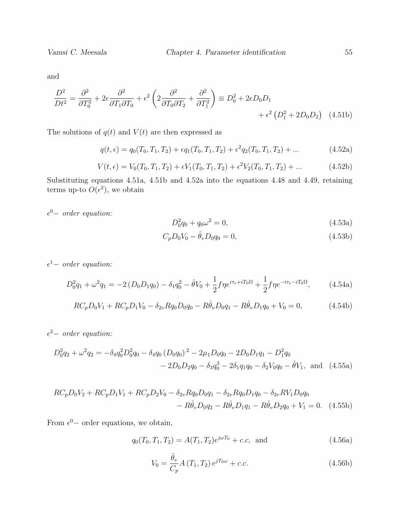
Vamsi C. Meesala Chapter 4. Parameter identification 55
and
D2
Dt2=
∂2
∂T 20
+ 2ε∂2
∂T1∂T0
+ ε2(
2∂2
∂T0∂T2
+∂2
∂T 21
)≡ D2
0 + 2εD0D1
+ ε2(D2
1 + 2D0D2
)(4.51b)
The solutions of q(t) and V (t) are then expressed as
q(t, ε) = q0(T0, T1, T2) + εq1(T0, T1, T2) + ε2q2(T0, T1, T2) + ... (4.52a)
V (t, ε) = V0(T0, T1, T2) + εV1(T0, T1, T2) + ε2V2(T0, T1, T2) + ... (4.52b)
Substituting equations 4.51a, 4.51b and 4.52a into the equations 4.48 and 4.49, retainingterms up-to O(ε2), we obtain
ε0− order equation:D2
0q0 + q0ω2 = 0, (4.53a)
CpD0V0 − θvD0q0 = 0, (4.53b)
ε1− order equation:
D20q1 + ω2q1 = −2 (D0D1q0)− δ1q
20 − θV0 +
1
2fηeiτe+iT0Ω +
1
2fηe−iτe−iT0Ω, (4.54a)
RCpD0V1 +RCpD1V0 − δ2vRq0D0q0 −RθvD0q1 −RθvD1q0 + V0 = 0, (4.54b)
ε2− order equation:
D20q2 + ω2q2 = −δ4q
20D
20q0 − δ4q0 (D0q0) 2 − 2µ1D0q0 − 2D0D1q1 −D2
1q0
− 2D0D2q0 − δ3q30 − 2δ1q1q0 − δ2V0q0 − θV1, and (4.55a)
RCpD0V2 +RCpD1V1 +RCpD2V0 − δ2vRq0D0q1 − δ2vRq0D1q0 − δ2vRV1D0q0
−RθvD0q2 −RθvD1q1 −RθvD2q0 + V1 = 0. (4.55b)
From ε0− order equations, we obtain,
q0(T0, T1, T2) = A(T1, T2)ejωT0 + c.c, and (4.56a)
V0 =θvCpA (T1, T2) ejT0ω + c.c. (4.56b)

Vamsi C. Meesala Chapter 4. Parameter identification 56
By substituting q0 and V0 in ε1− order equation 4.54a and eliminating secular terms weobtain
D1A =j
4ωCp
(2A1θθv − fηCpejτe+iσT1
)(4.57)
and solving for q1 and V1 yields
q1 = −Aδ1A
ω2+A2δ1e
2iT0ω
3ω2+ c.c, and (4.58a)
V1 =1
6Rω2C2p
[3δ2vRω
2CpA21e
2iT0ω + 2θv(A2
1δ1RCpe2iT0ω + 3iA1ωe
iT0ω)]
+ c.c. (4.58b)
Next, by using q1 and V1 in the ε2− order equation, 4.55a, and eliminating the secularterms, we obtain the relation for D2A. Using the relations for D1A and D2A, we obtain theamplitude and phase modulation equations as
A = εD1A+ ε2D2A (4.59)
writing the complex amplitude, A, in polar coordinates, A(T1, T2) = 12a(T0, T2)ejβ(T1,T2) and
defining γ = εσt+ τe − β to remove the explicit dependence of time in amplitude and phasemodulation equations, we obtain
a = −εfη(Ω− 3ω)
4ω2sin γ + ε2
[1
2a
(− θθvRω2C2
p
− 2µ1
)− fηθ2
8ω3Cpsin γ
], and (4.60)
γ = −ε
[−σ +
θθv2ωCp
+fη(Ω− 3ω)
4aω2cos γ
]
+ ε2
[a2 (6δ4ω
4 − 9δ3ω2 + 10δ2
1)
24ω3+
θ2θ2v
8ω3C2p
− fηθθv8aω3Cp
cos γ
]. (4.61)
To consider the steady state amplitude a0, for a given excitation, we set a = 0 and γ = 0and eliminate γ in equations 4.60 and 4.61 to obtain the following steady state amplituderesponse relation
16a20ω
2ε2(
2µ1Rω2C2
p + θθv
)2
f 2η2R2C2p
(2ωCp(3ω − Ω)− θεθv
)2
+a2
0
(−C2
p [a2ε (6δ4ω4 − 9δ3ω
2 + 10δ21) + 24σω3] + 12θω2Cpθv − 3θ2εθ2
v
)2
9f 2η2C2p
(2ωCp(3ω − Ω)− θεθv
)2 = 1 (4.62)
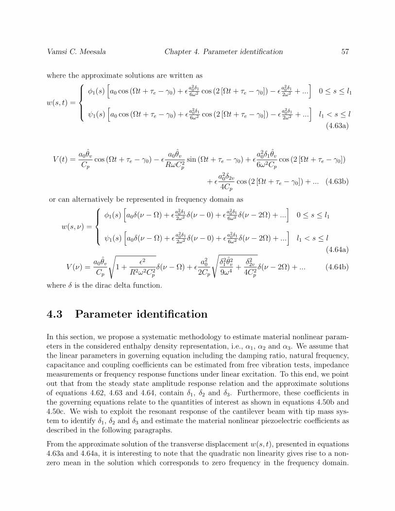
Vamsi C. Meesala Chapter 4. Parameter identification 57
where the approximate solutions are written as
w(s, t) =
φ1(s)
[a0 cos (Ωt+ τe − γ0) + ε
a20δ16ω2 cos (2 [Ωt+ τe − γ0])− εa
20δ1
2ω2 + ...]
0 ≤ s ≤ l1
ψ1(s)[a0 cos (Ωt+ τe − γ0) + ε
a20δ16ω2 cos (2 [Ωt+ τe − γ0])− εa
20δ1
2ω2 + ...]
l1 < s ≤ l
(4.63a)
V (t) =a0θvCp
cos (Ωt+ τe − γ0)− ε a0θvRωC2
p
sin (Ωt+ τe − γ0) + εa2
0δ1θv6ω2Cp
cos (2 [Ωt+ τe − γ0])
+ εa2
0δ2v
4Cpcos (2 [Ωt+ τe − γ0]) + ... (4.63b)
or can alternatively be represented in frequency domain as
w(s, ν) =
φ1(s)
[a0δ(ν − Ω) + ε
a20δ12ω2 δ(ν − 0) + ε
a20δ16ω2 δ(ν − 2Ω) + ...
]0 ≤ s ≤ l1
ψ1(s)[a0δ(ν − Ω) + ε
a20δ12ω2 δ(ν − 0) + ε
a20δ16ω2 δ(ν − 2Ω) + ...
]l1 < s ≤ l
(4.64a)
V (ν) =a0θvCp
√1 +
ε2
R2ω2C2p
δ(ν − Ω) + εa2
0
2Cp
√δ2
1 θ2v
9ω4+
δ22v
4C2p
δ(ν − 2Ω) + ... (4.64b)
where δ is the dirac delta function.
4.3 Parameter identification
In this section, we propose a systematic methodology to estimate material nonlinear param-eters in the considered enthalpy density representation, i.e., α1, α2 and α3. We assume thatthe linear parameters in governing equation including the damping ratio, natural frequency,capacitance and coupling coefficients can be estimated from free vibration tests, impedancemeasurements or frequency response functions under linear excitation. To this end, we pointout that from the steady state amplitude response relation and the approximate solutionsof equations 4.62, 4.63 and 4.64, contain δ1, δ2 and δ3. Furthermore, these coefficients inthe governing equations relate to the quantities of interest as shown in equations 4.50b and4.50c. We wish to exploit the resonant response of the cantilever beam with tip mass sys-tem to identify δ1, δ2 and δ3 and estimate the material nonlinear piezoelectric coefficients asdescribed in the following paragraphs.
From the approximate solution of the transverse displacement w(s, t), presented in equations4.63a and 4.64a, it is interesting to note that the quadratic non linearity gives rise to a non-zero mean in the solution which corresponds to zero frequency in the frequency domain.
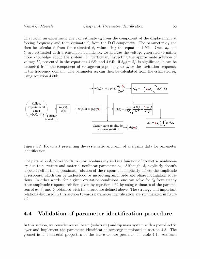
Vamsi C. Meesala Chapter 4. Parameter identification 58
That is, in an experiment one can estimate a0 from the component of the displacement atforcing frequency and then estimate δ1 from the D.C component. The parameter α1 canthen be calculated from the estimated δ1 value using the equation 4.50b. Once a0 andδ1 are estimated with a reasonable confidence, we analyze the voltage generated to gathermore knowledge about the system. In particular, inspecting the approximate solution ofvoltage V , presented in the equations 4.63b and 4.64b, if δ2v(≡ δ2) is significant, it can beextracted from the component of voltage corresponding to twice the excitation frequencyin the frequency domain. The parameter α3 can then be calculated from the estimated δ2v
using equation 4.50b.
w(s,ν), V(ν)
w(s,ν), V(ν)
w(s,Ω) = ϕ1(s)a0w(s,Ω) = ϕ1(s)a0
|w(s,0)| = ϵ ϕ1(s) |w(s,0)| = ϵ ϕ1(s)
V(2\Omega)V(2\Omega)
Fourier transform
Steady state amplitude response relation
δ3(α4)
Collect experimental
data : w(s,t), V(t)
Collect experimental
data : w(s,t), V(t)
Figure 4.2: Flowchart presenting the systematic approach of analyzing data for parameteridentification.
The parameter δ3 corresponds to cubic nonlinearity and is a function of geometric nonlinear-ity due to curvature and material nonlinear parameter α4. Although, δ3 explicitly doesn’tappear itself in the approximate solution of the response, it implicitly affects the amplitudeof response, which can be understood by inspecting amplitude and phase modulation equa-tions. In other words, for a given excitation conditions, one can solve for δ3 from steadystate amplitude response relation given by equation 4.62 by using estimates of the parame-ters of a0, δ1 and δ2 obtained with the procedure defined above. The strategy and importantrelations discussed in this section towards parameter identification are summarized in figure4.2.
4.4 Validation of parameter identification procedure
In this section, we consider a steel beam (substrate) and tip mass system with a piezoelectriclayer and implement the parameter identification strategy mentioned in section 4.3. Thegeometric and material properties of the harvester are presented in table 4.1. Assumed
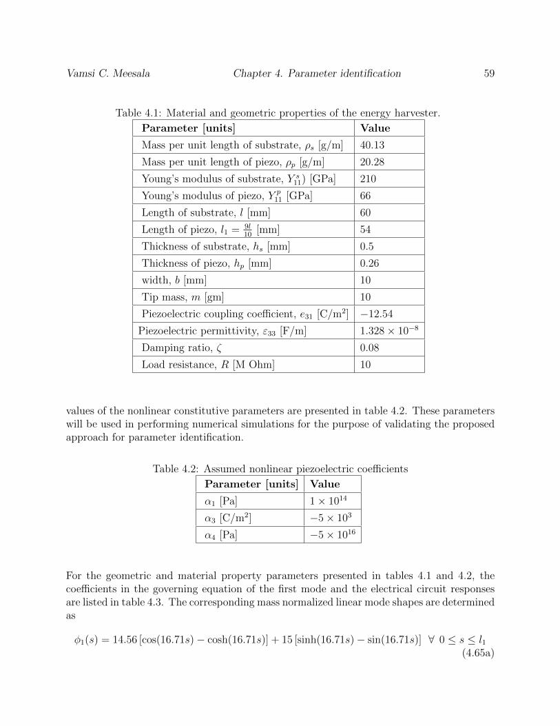
Vamsi C. Meesala Chapter 4. Parameter identification 59
Table 4.1: Material and geometric properties of the energy harvester.
Parameter [units] Value
Mass per unit length of substrate, ρs [g/m] 40.13
Mass per unit length of piezo, ρp [g/m] 20.28
Young’s modulus of substrate, Y s11) [GPa] 210
Young’s modulus of piezo, Y p11 [GPa] 66
Length of substrate, l [mm] 60
Length of piezo, l1 = 9l10
[mm] 54
Thickness of substrate, hs [mm] 0.5
Thickness of piezo, hp [mm] 0.26
width, b [mm] 10
Tip mass, m [gm] 10
Piezoelectric coupling coefficient, e31 [C/m2] −12.54
Piezoelectric permittivity, ε33 [F/m] 1.328× 10⁻⁸
Damping ratio, ζ 0.08
Load resistance, R [M Ohm] 10
values of the nonlinear constitutive parameters are presented in table 4.2. These parameterswill be used in performing numerical simulations for the purpose of validating the proposedapproach for parameter identification.
Table 4.2: Assumed nonlinear piezoelectric coefficients
Parameter [units] Value
α1 [Pa] 1× 10¹⁴
α3 [C/m2] −5× 10³
α4 [Pa] −5× 10¹⁶
For the geometric and material property parameters presented in tables 4.1 and 4.2, thecoefficients in the governing equation of the first mode and the electrical circuit responsesare listed in table 4.3. The corresponding mass normalized linear mode shapes are determinedas
φ1(s) = 14.56 [cos(16.71s)− cosh(16.71s)] + 15 [sinh(16.71s)− sin(16.71s)] ∀ 0 ≤ s ≤ l1(4.65a)
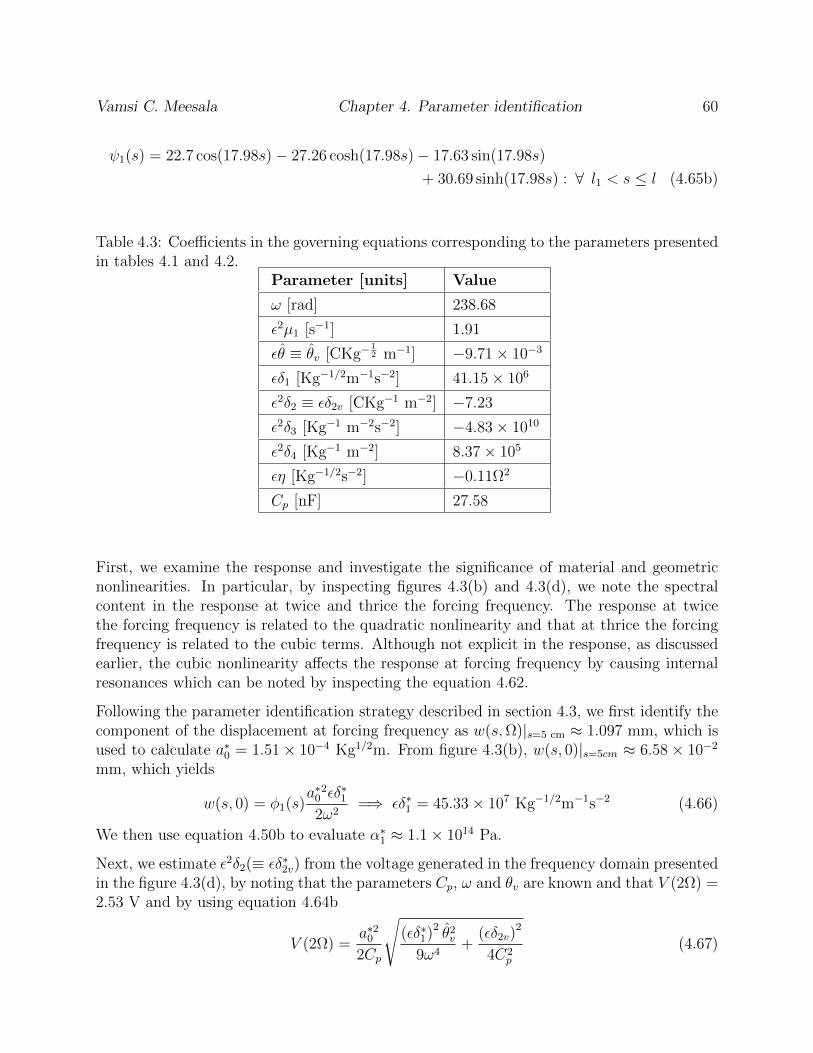
Vamsi C. Meesala Chapter 4. Parameter identification 60
ψ1(s) = 22.7 cos(17.98s)− 27.26 cosh(17.98s)− 17.63 sin(17.98s)
+ 30.69 sinh(17.98s) : ∀ l1 < s ≤ l (4.65b)
Table 4.3: Coefficients in the governing equations corresponding to the parameters presentedin tables 4.1 and 4.2.
Parameter [units] Value
ω [rad] 238.68
ε2µ1 [s−1] 1.91
εθ ≡ θv [CKg−12 m−1] −9.71× 10⁻³
εδ1 [Kg−1/2m−1s−2] 41.15× 10⁶
ε2δ2 ≡ εδ2v [CKg−1 m−2] −7.23
ε2δ3 [Kg−1 m−2s−2] −4.83× 10¹⁰
ε2δ4 [Kg−1 m−2] 8.37× 10⁵
εη [Kg−1/2s−2] −0.11Ω2
Cp [nF] 27.58
First, we examine the response and investigate the significance of material and geometricnonlinearities. In particular, by inspecting figures 4.3(b) and 4.3(d), we note the spectralcontent in the response at twice and thrice the forcing frequency. The response at twicethe forcing frequency is related to the quadratic nonlinearity and that at thrice the forcingfrequency is related to the cubic terms. Although not explicit in the response, as discussedearlier, the cubic nonlinearity affects the response at forcing frequency by causing internalresonances which can be noted by inspecting the equation 4.62.
Following the parameter identification strategy described in section 4.3, we first identify thecomponent of the displacement at forcing frequency as w(s,Ω)|s=5 cm ≈ 1.097 mm, which isused to calculate a∗0 = 1.51× 10⁻⁴ Kg1/2m. From figure 4.3(b), w(s, 0)|s=5cm ≈ 6.58× 10⁻²
mm, which yields
w(s, 0) = φ1(s)a∗0
2εδ∗12ω2
=⇒ εδ∗1 = 45.33× 10⁷ Kg−1/2m−1s−2 (4.66)
We then use equation 4.50b to evaluate α∗1 ≈ 1.1× 10¹⁴ Pa.
Next, we estimate ε2δ2(≡ εδ∗2v) from the voltage generated in the frequency domain presentedin the figure 4.3(d), by noting that the parameters Cp, ω and θv are known and that V (2Ω) =2.53 V and by using equation 4.64b
V (2Ω) =a∗20
2Cp
√(εδ∗1)2 θ2
v
9ω4+
(εδ2v)2
4C2p
(4.67)
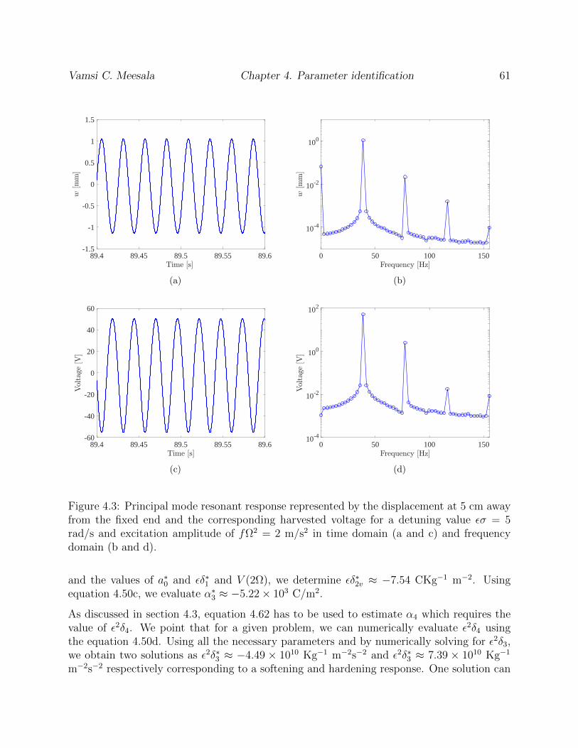
Vamsi C. Meesala Chapter 4. Parameter identification 61
89.4 89.45 89.5 89.55 89.6-1.5
-1
-0.5
0
0.5
1
1.5
(a)
0 50 100 150
10-4
10-2
100
(b)
89.4 89.45 89.5 89.55 89.6-60
-40
-20
0
20
40
60
(c)
0 50 100 15010-4
10-2
100
102
(d)
Figure 4.3: Principal mode resonant response represented by the displacement at 5 cm awayfrom the fixed end and the corresponding harvested voltage for a detuning value εσ = 5rad/s and excitation amplitude of fΩ2 = 2 m/s2 in time domain (a and c) and frequencydomain (b and d).
and the values of a∗0 and εδ∗1 and V (2Ω), we determine εδ∗2v ≈ −7.54 CKg−1 m−2. Usingequation 4.50c, we evaluate α∗3 ≈ −5.22× 10³ C/m2.
As discussed in section 4.3, equation 4.62 has to be used to estimate α4 which requires thevalue of ε2δ4. We point that for a given problem, we can numerically evaluate ε2δ4 usingthe equation 4.50d. Using all the necessary parameters and by numerically solving for ε2δ3,we obtain two solutions as ε2δ∗3 ≈ −4.49 × 10¹⁰ Kg−1 m−2s−2 and ε2δ∗3 ≈ 7.39 × 10¹⁰ Kg−1
m−2s−2 respectively corresponding to a softening and hardening response. One solution can
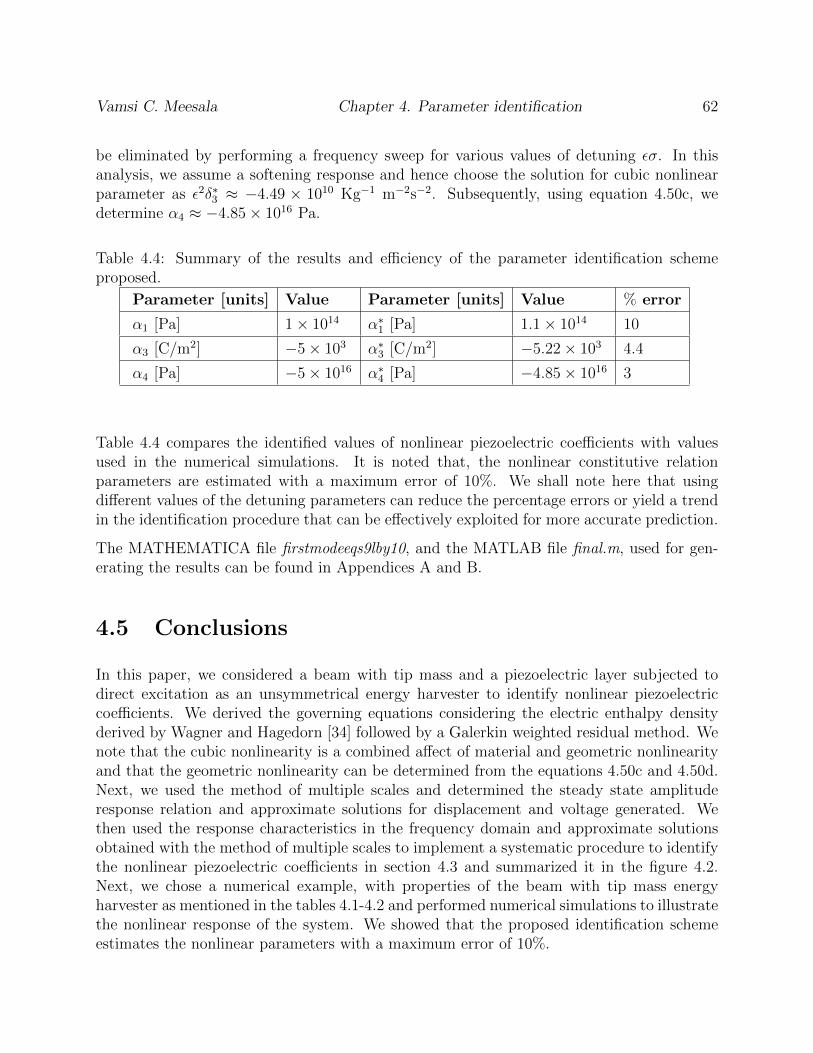
Vamsi C. Meesala Chapter 4. Parameter identification 62
be eliminated by performing a frequency sweep for various values of detuning εσ. In thisanalysis, we assume a softening response and hence choose the solution for cubic nonlinearparameter as ε2δ∗3 ≈ −4.49 × 10¹⁰ Kg−1 m−2s−2. Subsequently, using equation 4.50c, wedetermine α4 ≈ −4.85× 10¹⁶ Pa.
Table 4.4: Summary of the results and efficiency of the parameter identification schemeproposed.
Parameter [units] Value Parameter [units] Value % error
α1 [Pa] 1× 1014 α∗1 [Pa] 1.1× 10¹⁴ 10
α3 [C/m2] −5× 103 α∗3 [C/m2] −5.22× 10³ 4.4
α4 [Pa] −5× 1016 α∗4 [Pa] −4.85× 10¹⁶ 3
Table 4.4 compares the identified values of nonlinear piezoelectric coefficients with valuesused in the numerical simulations. It is noted that, the nonlinear constitutive relationparameters are estimated with a maximum error of 10%. We shall note here that usingdifferent values of the detuning parameters can reduce the percentage errors or yield a trendin the identification procedure that can be effectively exploited for more accurate prediction.
The MATHEMATICA file firstmodeeqs9lby10, and the MATLAB file final.m, used for gen-erating the results can be found in Appendices A and B.
4.5 Conclusions
In this paper, we considered a beam with tip mass and a piezoelectric layer subjected todirect excitation as an unsymmetrical energy harvester to identify nonlinear piezoelectriccoefficients. We derived the governing equations considering the electric enthalpy densityderived by Wagner and Hagedorn [34] followed by a Galerkin weighted residual method. Wenote that the cubic nonlinearity is a combined affect of material and geometric nonlinearityand that the geometric nonlinearity can be determined from the equations 4.50c and 4.50d.Next, we used the method of multiple scales and determined the steady state amplituderesponse relation and approximate solutions for displacement and voltage generated. Wethen used the response characteristics in the frequency domain and approximate solutionsobtained with the method of multiple scales to implement a systematic procedure to identifythe nonlinear piezoelectric coefficients in section 4.3 and summarized it in the figure 4.2.Next, we chose a numerical example, with properties of the beam with tip mass energyharvester as mentioned in the tables 4.1-4.2 and performed numerical simulations to illustratethe nonlinear response of the system. We showed that the proposed identification schemeestimates the nonlinear parameters with a maximum error of 10%.
Chapter 5
Conclusions and future work
In this work, we first presented theoretical modeling of a cantilever beam with tip masssystem subjected to parametric excitation. We showed that, though neglecting nonlinearboundary conditions can simplify the math in determining the governing equations, therepresentation of the response can be significantly altered. In particular, we demonstratedthat for the problem under consideration, the nature of the Hopf bifurcation is exactlyopposite and that the amplitude of the response is considerably different.
We then performed a sensitivity analysis of a cantilever beam with tip mass system subjectedto parametric excitation for small variations in the values of the elasticity and tip mass. Forthe problem considered, we illustrated that a decrease in elasticity and very small increase intip mass can alter the response of a system that is designed to yield a supercritical bifurcationto result in a sub-critical bifurcation. This observation can potentially be applied for usingparametrically excited micro-cantilever beams as sensing devices. We also noted that thesensitivity to small variations in the tip mass can be increased by decreasing σ.
Finally, we considered the cantilever beam with tip mass and a piezoelectric layer subjectedto direct excitation as an unsymmetrical energy harvester to identify nonlinear piezoelectriccoefficients. We derived the governing equations considering the electric enthalpy densityderived by Wagner and Hagedorn [34]. We then used the response characteristics in thefrequency domain and approximate solutions obtained with the method of multiple scalesto implement a systematic procedure to identify the nonlinear piezoelectric coefficients. Bychoosing a numerical example, we showed that the proposed identification scheme estimatesthe nonlinear parameters with a maximum error of 10%.
For future work, it is proposed that approaches and results presented here are to be validatedfurther with experiments and higher-fidelity models such as finite elements.
63

Appendix A
MATHEMATICA files
Below are the hyperlinked MATHEMATICA files:
• Genhamilton1.0
• mass vary
• mass vary 0p0096
• Genhamilton2.0
• firstmodeeqs9lby10
These above listed files are tested in MATHEMATICA 11.2 and 11.3.
64

Appendix B
MATLAB files
Below are the hyperlinked MATLAB files:
final.m, which needs the following two functions:
• ppx.m
• forced43peizoWHD9lby10.m
65
Bibliography
[1] Francois E Cellier and Jurgen Greifeneder. Continuous system modeling. SpringerScience & Business Media, 2013.
[2] Ali Hasan Nayfeh. Nonlinear interactions: analytical, computational and experimentalmethods. Wiley, 2000.
[3] Ali H Nayfeh and Balakumar Balachandran. Applied nonlinear dynamics: analytical,computational and experimental methods. John Wiley & Sons, 2008.
[4] Ali H Nayfeh and P Frank Pai. Linear and nonlinear structural mechanics. John Wiley& Sons, 2008.
[5] Lawrence N Virgin. Introduction to experimental nonlinear dynamics: a case study inmechanical vibration. Cambridge University Press, 2000.
[6] SK Dwivedy and RC Kar. Non-linear dynamics of a slender beam carrying a lumpedmass under principal parametric resonance with three-mode interactions. Internationaljournal of non-linear mechanics, 36(6):927–945, 2001.
[7] SK Dwivedy and RC Kar. Simultaneous combination and 1: 3: 5 internal resonancesin a parametrically excited beam–mass system. International journal of non-linearmechanics, 38(4):585–596, 2003.
[8] CWS To. The response of mast antenna structures to transient disturbances. PhDthesis, University of Southampton, 1979.
[9] CWS To. Vibration of a cantilever beam with a base excitation and tip mass. Journalof Sound and Vibration, 83(4):445–460, 1982.
[10] Kiun Kim and Thomas W Strganac. Nonlinear responses of a cantilever wing with anexternal store. In 44th AIAA Structures, Structural Dynamics, and Materials Confer-ence, Norfolk, VA, AIAA Paper, number 2003-1708, 2003.
[11] Philip S Beran, Thomas W Strganac, Kiun Kim, and Chetan Nichkawde. Studiesof store-induced limit-cycle oscillations using a model with full system nonlinearities.Nonlinear Dynamics, 37(4):323–339, 2004.
66

Vamsi C. Meesala Appendices 67
[12] LK Abbas, Q Chen, P Marzocca, and A Milanese. Non-linear aeroelastic investigationsof store (s)-induced limit cycle oscillations. Proceedings of the Institution of MechanicalEngineers, Part G: Journal of Aerospace Engineering, 222(1):63–80, 2008.
[13] AH Nayfeh, BK Hammad, and MR Hajj. Discretization effects on flutter aspects andcontrol of wing/store configurations. Journal of Vibration and Control, 18(7):1043–1055,2012.
[14] Ali H Nayfeh, Mehdi Ghommem, and Muhammad R Hajj. Normal form representationof the aeroelastic response of the goland wing. Nonlinear Dynamics, 67(3):1847–1861,2012.
[15] Sungsoo Na and Liviu Librescu. Dynamic response of adaptive cantilevers carry-ing external stores and subjected to blast loading. Journal of Sound and Vibration,231(4):1039–1055, 2000.
[16] Dongna Shen, Jyoti Ajitsaria, Song-Yul Choe, and Dong-Joo Kim. The optimal designand analysis of piezoelectric cantilever beams for power generation devices. MRS OnlineProceedings Library Archive, 888, 2005.
[17] Alper Erturk and Daniel J Inman. Piezoelectric energy harvesting. John Wiley & Sons,2011.
[18] Miso Kim, Mathias Hoegen, John Dugundji, and Brian L Wardle. Modeling and ex-perimental verification of proof mass effects on vibration energy harvester performance.Smart Materials and Structures, 19(4):045023, 2010.
[19] Mohammed F Daqaq, Christopher Stabler, Yousef Qaroush, and Thiago Seuaciuc-Osorio. Investigation of power harvesting via parametric excitations. Journal of In-telligent Material Systems and Structures, 20(5):545–557, 2009.
[20] A Abdelkefi, AH Nayfeh, and MR Hajj. Effects of nonlinear piezoelectric coupling onenergy harvesters under direct excitation. Nonlinear Dynamics, 67(2):1221–1232, 2012.
[21] Abdessattar Abdelkefi, Zhimiao Yan, and Muhammad R Hajj. Modeling and nonlinearanalysis of piezoelectric energy harvesting from transverse galloping. Smart materialsand Structures, 22(2):025016, 2013.
[22] Michael I Friswell, S Faruque Ali, Onur Bilgen, Sondipon Adhikari, Arthur W Lees,and Grzegorz Litak. Non-linear piezoelectric vibration energy harvesting from a verticalcantilever beam with tip mass. Journal of Intelligent Material Systems and Structures,23(13):1505–1521, 2012.
[23] Xinxin Li, Minhang Bao, Heng Yang, Shaoqun Shen, and Deren Lu. A micromachinedpiezoresistive angular rate sensor with a composite beam structure. Sensors and Actu-ators A: Physical, 72(3):217–223, 1999.
Vamsi C. Meesala Appendices 68
[24] Heng Yang, Minhang Bao, Hao Yin, and Shaoqun Shen. A novel bulk micromachinedgyroscope based on a rectangular beam-mass structure. Sensors and Actuators A: Phys-ical, 96(2):145–151, 2002.
[25] Rashid Bashir. Biomems: state-of-the-art in detection, opportunities and prospects.Advanced drug delivery reviews, 56(11):1565–1586, 2004.
[26] Sandeep Kumar Vashist. A review of microcantilevers for sensing applications. J. ofNanotechnology, 3:1–18, 2007.
[27] Blake N Johnson and Raj Mutharasan. Biosensing using dynamic-mode cantilever sen-sors: A review. Biosensors and bioelectronics, 32(1):1–18, 2012.
[28] Mai Duc Dai, Kilho Eom, and Chang-Wan Kim. Nanomechanical mass detection usingnonlinear oscillations. Applied Physics Letters, 95(20):203104, 2009.
[29] N Kacem, J Arcamone, F Perez-Murano, and S Hentz. Dynamic range enhancementof nonlinear nanomechanical resonant cantilevers for highly sensitive nems gas/masssensor applications. Journal of Micromechanics and Microengineering, 20(4):045023,2010.
[30] Wenhua Zhang, Rajashree Baskaran, and Kimberly L Turner. Effect of cubic nonlinear-ity on auto-parametrically amplified resonant mems mass sensor. Sensors and ActuatorsA: Physical, 102(1):139–150, 2002.
[31] Wenhua Zhang and Kimberly L Turner. Application of parametric resonance amplifica-tion in a single-crystal silicon micro-oscillator based mass sensor. Sensors and ActuatorsA: Physical, 122(1):23–30, 2005.
[32] N Aurelle, D Guyomar, C Richard, P Gonnard, and L Eyraud. Nonlinear behavior ofan ultrasonic transducer. Ultrasonics, 34(2-5):187–191, 1996.
[33] D Guyomar, N Aurelle, and L Eyraud. Piezoelectric ceramics nonlinear behavior. ap-plication to langevin transducer. Journal de Physique III, 7(6):1197–1208, 1997.
[34] U Von Wagner and P Hagedorn. Piezo–beam systems subjected to weak electricfield: experiments and modelling of non-linearities. Journal of Sound and Vibration,256(5):861–872, 2002.
[35] O Cuvalci and A Ertas. Pendulum as vibration absorber for flexible structures: exper-iments and theory. Journal of vibration and acoustics, 118(4):558–566, 1996.
[36] Zhimiao Yan and Muhammad R Hajj. Energy harvesting from an autoparametric vi-bration absorber. Smart Materials and Structures, 24(11):115012, 2015.
[37] Zhimiao Yan, Haithem E Taha, and Ting Tan. Nonlinear characteristics of an autopara-metric vibration system. Journal of Sound and Vibration, 390:1–22, 2017.
Vamsi C. Meesala Appendices 69
[38] Ivan Delgado-Velazquez. Nonlinear vibration of a cantilever beam. 2007.
[39] Perngjin F Pai and Ali H Nayfeh. Three-dimensional nonlinear vibrations of compositebeamsii. flapwise excitations. Nonlinear Dynamics, 2(1):1–34, 1991.
[40] TJ Anderson, AH Nayfeh, and B Balachandran. Experimental verification of the im-portance of the nonlinear curvature in the response of a cantilever beam. Journal ofVibration and Acoustics, 118(1):21–27, 1996.
[41] Ali H Nayfeh and Walter Lacarbonara. On the discretization of distributed-parametersystems with quadratic and cubic nonlinearities. Nonlinear Dynamics, 13(3):203–220,1997.
[42] Hiroshi Yabuno, Yoshiro Ide, and Nobuharu Aoshima. Nonlinear analysis of a paramet-rically excited cantilever beam: Effect of the tip mass on stationary response (specialissue on nonlinear dynamics). JSME International Journal Series C Mechanical Sys-tems, Machine Elements and Manufacturing, 41(3):555–562, 1998.
[43] Hiroshi Yabuno and Ali H Nayfeh. Nonlinear normal modes of a parametrically excitedcantilever beam. In Normal Modes and Localization in Nonlinear Systems, pages 65–77.Springer, 2001.
[44] Lawrence D Zavodney. A theoretical and experimental investigation of parametricallyexcited nonlinear mechanical systems. PhD thesis, Virginia Polytechnic Institute andState University, 1987.
[45] Samir A Emam and Ali H Nayfeh. Nonlinear responses of buckled beams tosubharmonic-resonance excitations. Nonlinear Dynamics, 35(2):105–122, 2004.
[46] Ali H Nayfeh. Introduction to perturbation techniques. John Wiley & Sons, 2011.
[47] Leonard Meirovitch. Fundamentals of vibrations. Waveland Press, 2010.
[48] C Chin and SA Nayfeh. Nonlinear normal modes of a cantilever beam. Journal ofvibration and acoustics, 117:477, 1995.
[49] AH Nayfeh and SA Nayfeh. Nonlinear normal modes of a continuous system withquadratic nonlinearities. TRANSACTIONS-AMERICAN SOCIETY OF MECHAN-ICAL ENGINEERS JOURNAL OF VIBRATION AND ACOUSTICS, 117:199–199,1995.
[50] Ali H Nayfeh and Dean T Mook. Nonlinear oscillations. John Wiley & Sons, 2008.
[51] Mohammad Ibrahim Younis and AH Nayfeh. A study of the nonlinear response of aresonant microbeam to an electric actuation. Nonlinear Dynamics, 31(1):91–117, 2003.
Vamsi C. Meesala Appendices 70
[52] Ali H Nayfeh. Resolving controversies in the application of the method of multiple scalesand the generalized method of averaging. Nonlinear Dynamics, 40(1):61–102, 2005.
[53] Nathan S Shenck and Joseph A Paradiso. Energy scavenging with shoe-mounted piezo-electrics. IEEE micro, 21(3):30–42, 2001.
[54] P Glynne-Jones, SP Beeby, EP James, and NM White. The modelling of a piezoelectricvibration powered generator for microsystems. In Transducers 01 Eurosensors XV,pages 46–49. Springer, 2001.
[55] Geffrey K Ottman, Heath F Hofmann, and George A Lesieutre. Optimized piezoelectricenergy harvesting circuit using step-down converter in discontinuous conduction mode.IEEE Transactions on power electronics, 18(2):696–703, 2003.
[56] Shad Roundy and Paul K Wright. A piezoelectric vibration based generator for wirelesselectronics. Smart Materials and structures, 13(5):1131, 2004.
[57] Daniel J Inman and Benjamin L Grisso. Towards autonomous sensing. In Smart Struc-tures and Materials 2006: Sensors and Smart Structures Technologies for Civil, Me-chanical, and Aerospace Systems, volume 6174, page 61740T. International Society forOptics and Photonics, 2006.
[58] Nader Jalili. Piezoelectric-based vibration control: from macro to micro/nano scalesystems. Springer Science & Business Media, 2009.
[59] Thomas Bailey and JE Ubbard. Distributed piezoelectric-polymer active vibration con-trol of a cantilever beam. Journal of Guidance, Control, and Dynamics, 8(5):605–611,1985.
[60] Nesbitt W Hagood and Andreas von Flotow. Damping of structural vibrations withpiezoelectric materials and passive electrical networks. Journal of Sound and Vibration,146(2):243–268, 1991.
[61] William W Clark. Vibration control with state-switched piezoelectric materials. Journalof intelligent material systems and structures, 11(4):263–271, 2000.
[62] Victor Giurgiutiu. Review of smart-materials actuation solutions for aeroelastic andvibration control. Journal of Intelligent Material Systems and Structures, 11(7):525–544, 2000.
[63] Liviu Librescu and Sungsoo Na. Active vibration control of doubly tapered thin-walledbeams using piezoelectric actuation. Thin-Walled Structures, 39(1):65–82, 2001.
[64] SO Reza Moheimani. A survey of recent innovations in vibration damping and controlusing shunted piezoelectric transducers. IEEE transactions on control systems technol-ogy, 11(4):482–494, 2003.
Vamsi C. Meesala Appendices 71
[65] Alper Erturk, Jamil M Renno, and Daniel J Inman. Modeling of piezoelectric energyharvesting from an l-shaped beam-mass structure with an application to uavs. Journalof intelligent material systems and structures, 20(5):529–544, 2009.
[66] Samuel C Stanton, Clark C McGehee, and Brian P Mann. Nonlinear dynamics forbroadband energy harvesting: Investigation of a bistable piezoelectric inertial generator.Physica D: Nonlinear Phenomena, 239(10):640–653, 2010.
[67] S Adhikari, MI Friswell, and DJ Inman. Piezoelectric energy harvesting from broadbandrandom vibrations. Smart Materials and Structures, 18(11):115005, 2009.
[68] AF Arrieta, P Hagedorn, Alper Erturk, and DJ Inman. A piezoelectric bistable plate fornonlinear broadband energy harvesting. Applied Physics Letters, 97(10):104102, 2010.
[69] Masato Abe, Gyuhae Park, and Daniel J Inman. Impedance-based monitoring of stressin thin structural members. UNIT 45002 APO AP 96337-5002, page 285, 2001.
[70] Gyuhae Park, Hoon Sohn, Charles R Farrar, Daniel J Inman, et al. Overview of piezo-electric impedance-based health monitoring and path forward. Shock and VibrationDigest, 35(6):451–464, 2003.
[71] Mohsen Safaei and Steven R Anton. Sensing and energy harvesting performance, andfatigue life of embedded piezoelectric transducer in total knee arthroplasty. In ASME2016 Conference on Smart Materials, Adaptive Structures and Intelligent Systems, pagesV002T07A010–V002T07A010. American Society of Mechanical Engineers, 2016.
[72] Elias Hoummadi, Mohsen Safaei, and Steven R Anton. Design, analysis, and fabricationof a piezoelectric force plate. In Health Monitoring of Structural and Biological Systems2017, volume 10170, page 101700W. International Society for Optics and Photonics,2017.
[73] Teimour Maleki, Ning Cao, Seung Hyun Song, Chinghai Kao, Song-Chu Ko, and BabakZiaie. An ultrasonically powered implantable micro-oxygen generator (imog). IEEEtransactions on Biomedical Engineering, 58(11):3104–3111, 2011.
[74] Maurice GL Roes, Jorge L Duarte, Marcel AM Hendrix, and Elena A Lomonova. Acous-tic energy transfer: A review. IEEE Transactions on Industrial Electronics, 60(1):242–248, 2013.
[75] S Shahab, M Gray, and A Erturk. Ultrasonic power transfer from a spherical acousticwave source to a free-free piezoelectric receiver: Modeling and experiment. Journal ofApplied Physics, 117(10):104903, 2015.
[76] Mohammed F Daqaq, Ravindra Masana, Alper Erturk, and D Dane Quinn. On therole of nonlinearities in vibratory energy harvesting: a critical review and discussion.Applied Mechanics Reviews, 66(4):040801, 2014.
Vamsi C. Meesala Bibliography 72
[77] S Leadenham and A Erturk. M-shaped asymmetric nonlinear oscillator for broadbandvibration energy harvesting: Harmonic balance analysis and experimental validation.Journal of Sound and Vibration, 333(23):6209–6223, 2014.
[78] RL Harne and KW Wang. A review of the recent research on vibration energy harvestingvia bistable systems. Smart materials and structures, 22(2):023001, 2013.
[79] Stephen Leadenham and Alper Erturk. Unified nonlinear electroelastic dynamics of abimorph piezoelectric cantilever for energy harvesting, sensing, and actuation. NonlinearDynamics, 79(3):1727–1743, 2015.
[80] Ali H Nayfeh. Parametric identification of nonlinear dynamic systems. In Advances andTrends in Structures and Dynamics, pages 487–493. Elsevier, 1985.
[81] Lawrence D Zavodney. Identification of nonlinearity in structural systems: Theory,simulation, and experiment. Applied Mechanics Reviews, 44(11S):S295–S303, 1991.
[82] MR Hajj, J Fung, AH Nayfeh, and SO’F Fahey. Damping identification using pertur-bation techniques and higher-order spectra. Nonlinear Dynamics, 23(2):189–203, 2000.
[83] Gaetan Kerschen, Keith Worden, Alexander F Vakakis, and Jean-Claude Golinval. Past,present and future of nonlinear system identification in structural dynamics. Mechanicalsystems and signal processing, 20(3):505–592, 2006.
[84] F Ayela and T Fournier. An experimental study of anharmonic micromachined siliconresonators. Measurement Science and Technology, 9(11):1821, 1998.
[85] AJ Dick, B Balachandran, DL DeVoe, and CD Mote Jr. Parametric identification ofpiezoelectric microscale resonators. Journal of Micromechanics and Microengineering,16(8):1593, 2006.
[86] Stephen H Crandall. Dynamics of mechanical and electromechanical systems. McGraw-Hill, 1968.
[87] Nesbitt W Hagood, Walter H Chung, and Andreas Von Flotow. Modelling of piezo-electric actuator dynamics for active structural control. Journal of Intelligent MaterialSystems and Structures, 1(3):327–354, 1990.
[88] Henry Angelo Sodano. Macro-fiber composites for sensing, actuation and power gener-ation. PhD thesis, Virginia Tech, 2003.
[89] Steven Robert Anton. Multifunctional piezoelectric energy harvesting concepts. PhDthesis, Virginia Tech, 2011.