Embed Size (px)
Citation preview

MLU for Windows
Well flow modeling in multilayer aquifer systems
MLU
Aquifer and Pump Test Analysis Software
Slug test analysis and Step drawdown test analysis
Analytical groundwater flow modelling and pumping test simulations
Confined Aquifer, Unconfined Aquifer, Leaky Aquifer
Kick Hemker & Vincent Post
Amsterdam
www.microfem.com
2
MLU for Windows
CONTENTS
Introduction . . . . . . . . . . . . . . . . . . . . . . . . . . . . . . . . . . . . . . . . . . . . . . . . . . . . . . . 3
Solution Method . . . . . . . . . . . . . . . . . . . . . . . . . . . . . . . . . . . . . . . . . . . . . 3 Application. . . . . . . . . . . . . . . . . . . . . . . . . . . . . . . . . . . . . . . . . . . . . . . . . . 4 MLU versus numerical models . . . . . . . . . . . . . . . . . . . . . . . . . . . . . . . . . . 4 Software capacity . . . . . . . . . . . . . . . . . . . . . . . . . . . . . . . . . . . . . . . . . . . . 5 Data input . . . . . . . . . . . . . . . . . . . . . . . . . . . . . . . . . . . . . . . . . . . . . . . . . . 5 Inverse modeling . . . . . . . . . . . . . . . . . . . . . . . . . . . . . . . . . . . . . . . . . . . . 5 Data output . . . . . . . . . . . . . . . . . . . . . . . . . . . . . . . . . . . . . . . . . . . . . . . . . 5 Graphical output . . . . . . . . . . . . . . . . . . . . . . . . . . . . . . . . . . . . . . . . . . . . . 5 Free try-out version . . . . . . . . . . . . . . . . . . . . . . . . . . . . . . . . . . . . . . . . . . . 6 Review in Ground Water . . . . . . . . . . . . . . . . . . . . . . . . . . . . . . . . . . . . . . . 6 Price and orders . . . . . . . . . . . . . . . . . . . . . . . . . . . . . . . . . . . . . . . . . . . . . 6 Free updates and User support . . . . . . . . . . . . . . . . . . . . . . . . . . . . . . . . . . 6
User instructions . . . . . . . . . . . . . . . . . . . . . . . . . . . . . . . . . . . . . . . . . . . . . . . . . . . 7 Installing and running MLU . . . . . . . . . . . . . . . . . . . . . . . . . . . . . . . . . . . . 7 Data input 1: General info . . . . . . . . . . . . . . . . . . . . . . . . . . . . . . . . . . . . . 8 Data input 2: Aquifer system . . . . . . . . . . . . . . . . . . . . . . . . . . . . . . . . . . . 9 Data input 3: Pumping wells . . . . . . . . . . . . . . . . . . . . . . . . . . . . . . . . . . . 11 Data input 4: Observation wells . . . . . . . . . . . . . . . . . . . . . . . . . . . . . . . . . 13 Results: Parameter optimization . . . . . . . . . . . . . . . . . . . . . . . . . . . . . . . . . 14 Results: Time graphs . . . . . . . . . . . . . . . . . . . . . . . . . . . . . . . . . . . . . . . . . 17 Results: Contour plot . . . . . . . . . . . . . . . . . . . . . . . . . . . . . . . . . . . . . . . . . 19 Import: Import image files . . . . . . . . . . . . . . . . . . . . . . . . . . . . . . . . . . . . . 20 Export: Save curves as FTH . . . . . . . . . . . . . . . . . . . . . . . . . . . . . . . . . . . 21 Export: Save contours as XYZ . . . . . . . . . . . . . . . . . . . . . . . . . . . . . . . . . 21 Export: Save model as FEM . . . . . . . . . . . . . . . . . . . . . . . . . . . . . . . . . . . 22
Verification tests and Example models . . . . . . . . . . . . . . . . . . . . . . . . . . . . . . . . . 23 Main characteristics of the example models . . . . . . . . . . . . . . . . . . . . . . . 24
Optimization results Example Schroth.mlu . . . . . . . . . . . . . . . . . . . . . . . 27 MLU data file layout . . . . . . . . . . . . . . . . . . . . . . . . . . . . . . . . . . . . . . . . . . . . . . . 28 References . . . . . . . . . . . . . . . . . . . . . . . . . . . . . . . . . . . . . . . . . . . . . . . . . . . . . . 29 License agreement . . . . . . . . . . . . . . . . . . . . . . . . . . . . . . . . . . . . . . . . . . . . . . . . . 30
3
INTRODUCTION MLU for Windows is a groundwater modeling tool to compute drawdowns, analyze well flow and aquifer test data, and design well fields. MLU for Windows combines:
• An innovative analytical solution technique for well flow in layered aquifer systems
• Stehfest’s numerical method to convert the solution from the Laplace domain into the real domain
• The superposition principle, both in space (multiple wells) and time (variable discharges)
• The Levenberg-Marquardt algorithm for parameter optimization (automated curve fitting).
This unique combination of techniques allows all tests to be analyzed in a consistent way with a single user interface. Results are printed in ASCII files and plotted as time-drawdown graphs and animated contour plots.
Solution Method
As a rule present day software for aquifer and slug test analysis still use the same analytical solutions and techniques that were common several decades ago. Each type of test, characterized by a long list of conditions and assumptions, is associated with a particular analytical solution (e.g. Theis, Hantush, Neuman, Boulton, Papadopulos, Moench, Bouwer-Rice) for usually one or sometimes two aquifers. The related procedures to determine the aquifer hydraulic properties often require straight line fitting or type curve matching with some part of the measured data. Unlike traditional aquifer test software, MLU is based on a single analytical solution technique for well flow that handles:
• Layered aquifer systems, i.e. multi-aquifer systems (aquifers and aquitards) and single layered stratified aquifers (Fig. 1)
• Confined, leaky and delayed yield systems
• Effects of aquifer and aquitard storativities
• One or more pumping or injection wells
• One or more pumping periods for each well
• Finite diameter well screens in any selection of aquifer layers
• Well bore storage and skin effect for each pumping well
• Delayed observation well response
• Individual and grouped parameters to be determined in one run.
Theoretical background information on the applied analytical solution techniques for multiple aquifer systems has been published in: Journal of Hydrology 90, p. 231-249 (1987) and 225: p. 1-18 and p. 19-44 (1999). The non-linear regression technique is described in Ground Water (1985) 23, no.2, p. 247-253. See the references for further details.
4
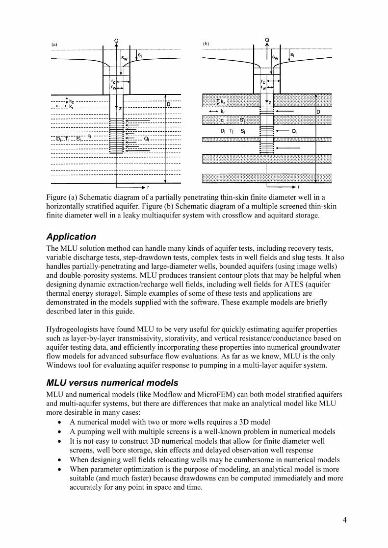
Figure (a) Schematic diagram of a partially penetrating thin-skin finite diameter well in a horizontally stratified aquifer. Figure (b) Schematic diagram of a multiple screened thin-skin finite diameter well in a leaky multiaquifer system with crossflow and aquitard storage.
Application
The MLU solution method can handle many kinds of aquifer tests, including recovery tests, variable discharge tests, step-drawdown tests, complex tests in well fields and slug tests. It also handles partially-penetrating and large-diameter wells, bounded aquifers (using image wells) and double-porosity systems. MLU produces transient contour plots that may be helpful when designing dynamic extraction/recharge well fields, including well fields for ATES (aquifer thermal energy storage). Simple examples of some of these tests and applications are demonstrated in the models supplied with the software. These example models are briefly described later in this guide. Hydrogeologists have found MLU to be very useful for quickly estimating aquifer properties such as layer-by-layer transmissivity, storativity, and vertical resistance/conductance based on aquifer testing data, and efficiently incorporating these properties into numerical groundwater flow models for advanced subsurface flow evaluations. As far as we know, MLU is the only Windows tool for evaluating aquifer response to pumping in a multi-layer aquifer system.
MLU versus numerical models
MLU and numerical models (like Modflow and MicroFEM) can both model stratified aquifers and multi-aquifer systems, but there are differences that make an analytical model like MLU more desirable in many cases:
• A numerical model with two or more wells requires a 3D model
• A pumping well with multiple screens is a well-known problem in numerical models
• It is not easy to construct 3D numerical models that allow for finite diameter well screens, well bore storage, skin effects and delayed observation well response
• When designing well fields relocating wells may be cumbersome in numerical models
• When parameter optimization is the purpose of modeling, an analytical model is more suitable (and much faster) because drawdowns can be computed immediately and more accurately for any point in space and time.
5
On the other hand MLU models have some important restrictions:
• All layers are assumed homogeneous, isotropic and of infinite extent
• Only groundwater flow resulting from pumping and injection wells can be modeled.
Software capacity
The MLU software can handle:
• 80 aquifers (layers) and 81 aquitards
• 1000 pumping/injection wells
• 100 pumping periods per well
• 100 observation wells
• 1000 measured drawdowns per observation well
• 16 parameters to be optimized in one run.
Data input
• Interactive input
• Data exchange with spreadsheets (copy & paste)
• Modify MLU input data file (ASCII)
• Time conversion: seconds, minutes, hours, days and years.
• Length conversion: meters, feet.
Inverse modeling
• Individual and grouped parameters can be determined in one run
• Automated curve fitting is based on the Levenberg-Marquardt algorithm
• Linear and log-transformed least squares solutions
• Statistical data output includes standard deviations and correlation matrix
• Parameter optimization and final output results in ASCII-files.
Data output
• Data exchange with spreadsheets (copy & paste)
• MLU data file (ASCII)
• Optimization results, including calculated and observed drawdowns (ASCII)
• Data file that contains computed heads of displayed time graph (FTH-file)
• Data file that contains computed drawdowns of displayed contour map (XYZ-file)
• Data file that contains a MicroFEM finite element model (FEM-file).
Graphical output
• Linear, semi-log and log-log time graphs of drawdown or head
• Time-variant aquifer discharge at a well screened over multiple aquifers
• Animated contour plots of drawdown and build-up cones
• Clipboard bitmap output and vector-based meta-file output.

6
Free try-out version
The MLU-LT version is a reduced (lite) version of MLU for Windows, and is available for teaching, testing and the analysis of simple aquifer tests. The LT version is free, but the application is limited to two aquifer models and two wells. The LT version can be downloaded from the MicroFEM web site: http://www.microfem.com MLU-LT can handle:
• 2 aquifers and 3 aquitards
• 2 pumping/injection wells
• 5 observation wells
• 6 parameters to be optimized in one run.
Review in Ground Water
MLU for Windows has been reviewed by the NGWA Ground Water Journal in the Software Spotlight Column, which is edited by Chunmiao Zheng, Ground Water 50, No. 4, p. 504-510. It received the following ratings on the scale of 1 (worst) to 5 (best):
• Capability 4.8
• Reliability 4.5
• Ease of use 4.0
• Tech support 5.0
Price and orders
A site license for the Windows-based version of MLU costs €490 (about 625 US$). Order directly from the web site: http://www.microfem.com/order/index.html, or e-mail the authors: [email protected]
Free updates and User support
There are no annual recurring costs. Regular updates (improvements and small extensions) are free. Customer login allows all licensed users to download the latest update anytime. User support is provided by the developers free of charge: [email protected].

7
USER INSTRUCTIONS
Installing and running MLU
Installing: Unzip the MLU….zip file, double-click the exe-file and follow the installation instructions. Starting: Double-click the MLU icon. The MLU window includes standard components:
• Title bar
• Menu bar: File, Edit, View, Calculate, Export, Windows, Help
• Tool bar with buttons: New, Open, Save, Cut, Copy, Paste, Optimize
• Seven tabs to access the data input and result screens
• Status bar. Menu commands: File: New (start a new project), Open (load an existing MLU project file), Reopen, Save, Save as …, Close (close the current project), Exit (close MLU) Edit: Cut, Copy, Paste, Delete row(s), Insert row(s), Clear, Select all View: Status bar, Toolbar, Background images Calculate: Optimize, Preferences Import Import image files Export: Copy time graph, Copy contour plot, Save curves as FTH, Save contours as XYZ, Save model as FEM Windows: Cascade, Tile horizontally, Tile vertically, Minimize all, Arrange all Help: MLU Help, MLU on the web, About…. MLU Help as well as <F1> activate the Help system and display help texts corresponding with one of the following tabs: Tabs 1 through 7: 1 - Data input: General information 2 - Data input: Aquifer system 3 - Data input: Pumping wells 4 - Data input: Observation wells 5 - Results: Optimization results 6 - Results: Time graphs 7 - Results: Contour plot. Start a new project by pressing the Toolbar “New” button or File | New and fill out the four input screen pages (tabs 1 through 4). Or open an existing project by pressing the Toolbar “Open” button or File | Open. MLU can handle multiple open projects at the same time.
8
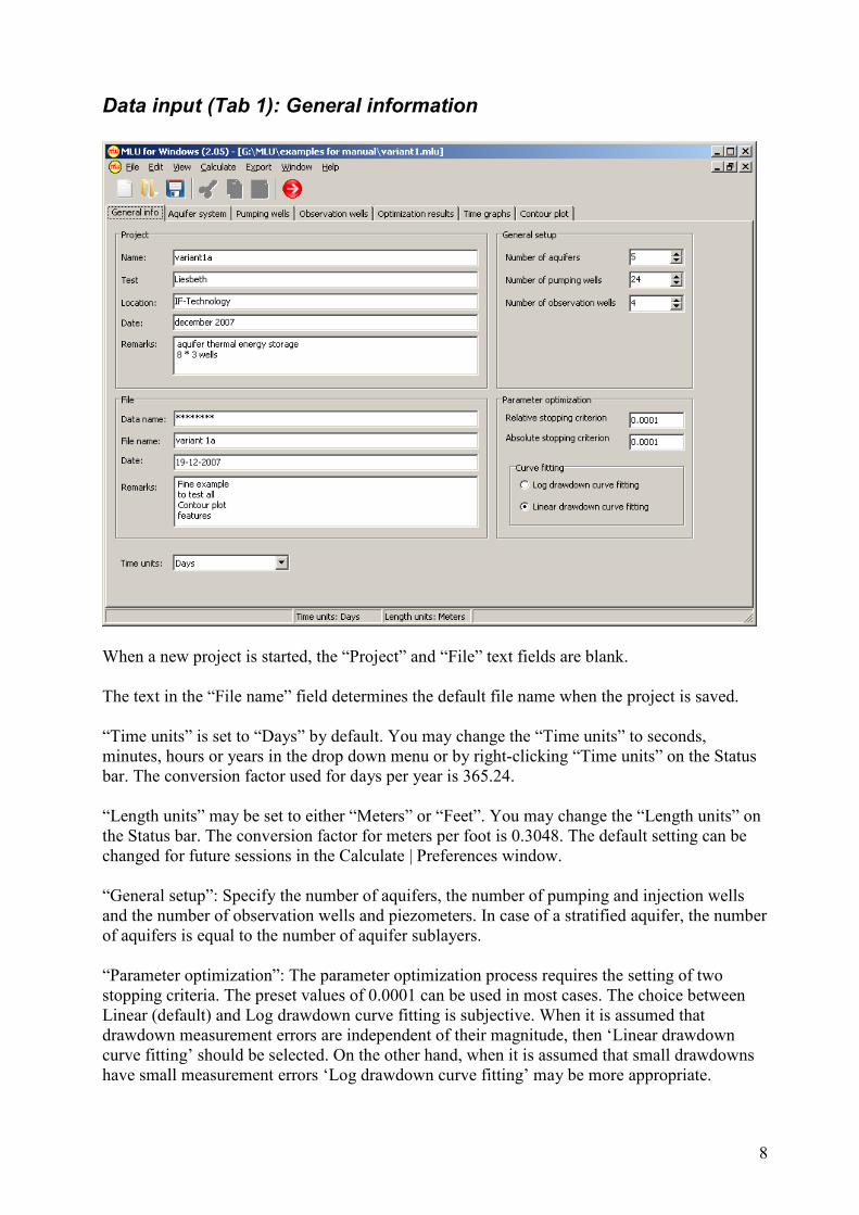
Data input (Tab 1): General information
When a new project is started, the “Project” and “File” text fields are blank. The text in the “File name” field determines the default file name when the project is saved. “Time units” is set to “Days” by default. You may change the “Time units” to seconds, minutes, hours or years in the drop down menu or by right-clicking “Time units” on the Status bar. The conversion factor used for days per year is 365.24. “Length units” may be set to either “Meters” or “Feet”. You may change the “Length units” on the Status bar. The conversion factor for meters per foot is 0.3048. The default setting can be changed for future sessions in the Calculate | Preferences window. “General setup”: Specify the number of aquifers, the number of pumping and injection wells and the number of observation wells and piezometers. In case of a stratified aquifer, the number of aquifers is equal to the number of aquifer sublayers. “Parameter optimization”: The parameter optimization process requires the setting of two stopping criteria. The preset values of 0.0001 can be used in most cases. The choice between Linear (default) and Log drawdown curve fitting is subjective. When it is assumed that drawdown measurement errors are independent of their magnitude, then ‘Linear drawdown curve fitting’ should be selected. On the other hand, when it is assumed that small drawdowns have small measurement errors ‘Log drawdown curve fitting’ may be more appropriate.
9
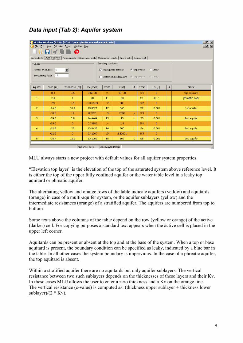
Data input (Tab 2): Aquifer system
MLU always starts a new project with default values for all aquifer system properties. “Elevation top layer” is the elevation of the top of the saturated system above reference level. It is either the top of the upper fully confined aquifer or the water table level in a leaky top aquitard or phreatic aquifer. The alternating yellow and orange rows of the table indicate aquifers (yellow) and aquitards (orange) in case of a multi-aquifer system, or the aquifer sublayers (yellow) and the intermediate resistances (orange) of a stratified aquifer. The aquifers are numbered from top to bottom. Some texts above the columns of the table depend on the row (yellow or orange) of the active (darker) cell. For copying purposes a standard text appears when the active cell is placed in the upper left corner. Aquitards can be present or absent at the top and at the base of the system. When a top or base aquitard is present, the boundary condition can be specified as leaky, indicated by a blue bar in the table. In all other cases the system boundary is impervious. In the case of a phreatic aquifer, the top aquitard is absent. Within a stratified aquifer there are no aquitards but only aquifer sublayers. The vertical resistance between two such sublayers depends on the thicknesses of these layers and their Kv. In these cases MLU allows the user to enter a zero thickness and a Kv on the orange line. The vertical resistance (c-value) is computed as: (thickness upper sublayer + thickness lower sublayer)/(2 * Kv).
10
Used codes: T1, T2, … : Transmissivities of aquifers or sublayers = thickness * Kh, [m2/day, ft2/sec, etc.] Kh: horizontal hydraulic conductivity of an aquifer or stratified aquifer sublayer c1, c2, … : Vertical resistances (inverse of conductance) = thickness / Kv, [day, sec, etc.] Kv: vertical hydraulic conductivity of an aquitard (multi-aquifer system) or the average between the middles of two adjacent stratified aquifer sublayers S1, S2, … : Storativities of aquifers or sublayers [-] S’1, S’2, ..: Storativities of aquitards [-]. #-columns: Use any non-zero character (A .. Z, a .. z, 1 .. 9) to indicate that the current system property is a parameter to be optimized. Two or more parameters that must be optimized as a group (i.e. the same multiplication factor will be applied) must be marked with the same character. If the entry is blank the current parameter will be kept constant during optimization. Zero-valued properties (storativity) cannot be optimized. When entering new data in the table, some other values in the table will be updated according to the following rules:
• New input of "base" (if smaller than value above) changes "thickness". It also changes the "base" of all lower layers
• New input of "thickness" changes "base" of the same and all lower layers
• New input of "thickness" or "base" changes "Kv or Kh" of that layer, but leaves "c", "T", "S" and "S' " unaltered
• New input of "Kv" or "Kh" changes "c" or "T"
• New input and optimization of "c" or "T" changes "Kv" or "Kh"
• New input and optimization of "S" or "S' " has no effect on other values in the table. And in case of a zero-thickness resistance layer (i.e. within a stratified aquifer)
• New input of “thickness” or "base" of a layer not only changes “Kh” of that layer, but also “Kv” of the adjacent zero-thickness layer(s).
11
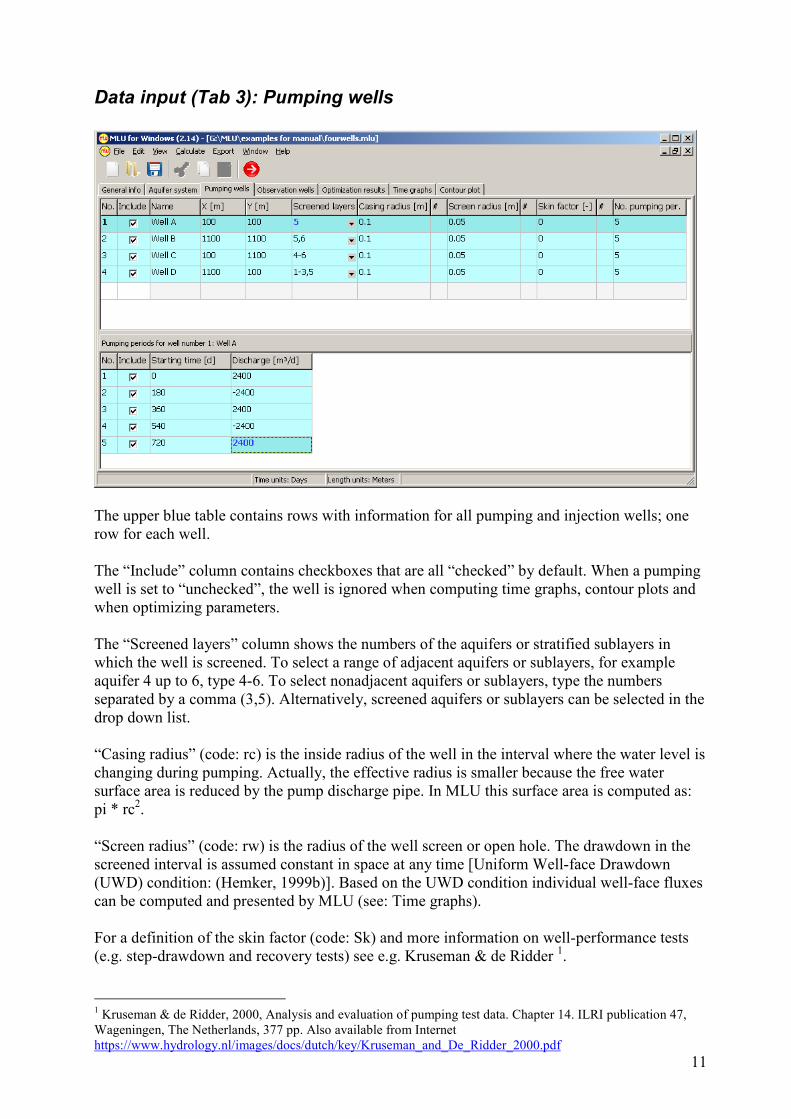
Data input (Tab 3): Pumping wells
The upper blue table contains rows with information for all pumping and injection wells; one row for each well. The “Include” column contains checkboxes that are all “checked” by default. When a pumping well is set to “unchecked”, the well is ignored when computing time graphs, contour plots and when optimizing parameters. The “Screened layers” column shows the numbers of the aquifers or stratified sublayers in which the well is screened. To select a range of adjacent aquifers or sublayers, for example aquifer 4 up to 6, type 4-6. To select nonadjacent aquifers or sublayers, type the numbers separated by a comma (3,5). Alternatively, screened aquifers or sublayers can be selected in the drop down list. “Casing radius” (code: rc) is the inside radius of the well in the interval where the water level is changing during pumping. Actually, the effective radius is smaller because the free water surface area is reduced by the pump discharge pipe. In MLU this surface area is computed as: pi * rc2. “Screen radius” (code: rw) is the radius of the well screen or open hole. The drawdown in the screened interval is assumed constant in space at any time [Uniform Well-face Drawdown (UWD) condition: (Hemker, 1999b)]. Based on the UWD condition individual well-face fluxes can be computed and presented by MLU (see: Time graphs). For a definition of the skin factor (code: Sk) and more information on well-performance tests (e.g. step-drawdown and recovery tests) see e.g. Kruseman & de Ridder 1.
1 Kruseman & de Ridder, 2000, Analysis and evaluation of pumping test data. Chapter 14. ILRI publication 47, Wageningen, The Netherlands, 377 pp. Also available from Internet https://www.hydrology.nl/images/docs/dutch/key/Kruseman_and_De_Ridder_2000.pdf

12
#-columns: Well characteristics (casing radius, screen radius and skin factor) may also be optimized. Use any non-zero character (A .. Z, a .. z, 1 .. 9) to indicate that the well characteristic is a parameter to be optimized. Two or more parameters that must be optimized as a group (i.e. the same multiplication factor will be applied) must be marked by the same character. Well characteristics cannot be grouped with aquifer system properties. Zero-valued well characteristics (casing radius, skin factor) cannot be optimized. The “No. pumping per.” column is used to indicate the number of constant discharge pumping periods. This number must be 1 or larger (up to 100), and determines the number of rows in the lower table. The lower table shows how the pumping rate of the well selected in the upper table changes in time, by specifying the starting time and the constant discharge rate of each period. Injection rates are specified by negative discharges, while the discharge rate of a recovery period is zero. Unchecked pumping (or injection) periods are ignored when computing time graphs, contour plots, and optimizing parameters. The table of pumping periods is expanded automatically when pasted blocks appear to be too large to fit within the available rows. The bar between the tables can be shifted upward and downward.
13
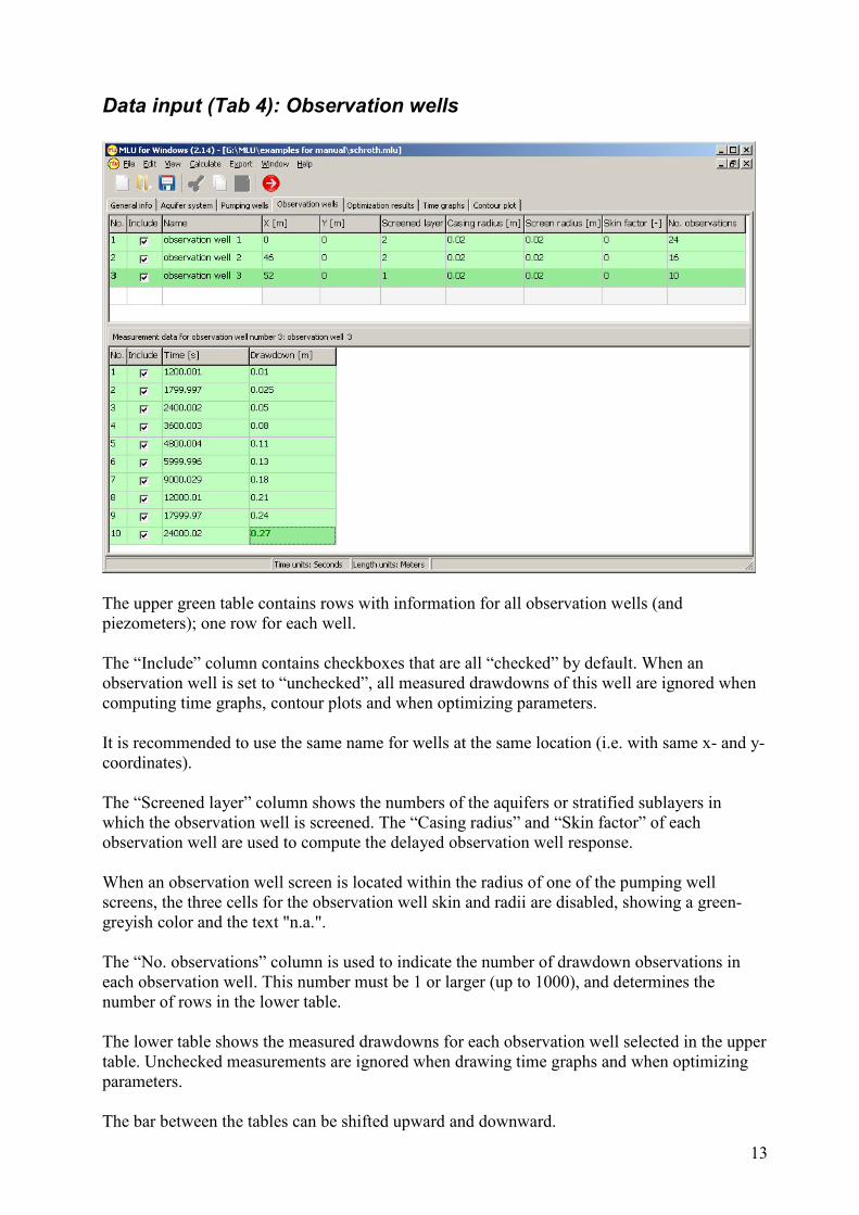
Data input (Tab 4): Observation wells
The upper green table contains rows with information for all observation wells (and piezometers); one row for each well. The “Include” column contains checkboxes that are all “checked” by default. When an observation well is set to “unchecked”, all measured drawdowns of this well are ignored when computing time graphs, contour plots and when optimizing parameters. It is recommended to use the same name for wells at the same location (i.e. with same x- and y-coordinates). The “Screened layer” column shows the numbers of the aquifers or stratified sublayers in which the observation well is screened. The “Casing radius” and “Skin factor” of each observation well are used to compute the delayed observation well response. When an observation well screen is located within the radius of one of the pumping well screens, the three cells for the observation well skin and radii are disabled, showing a green-greyish color and the text "n.a.". The “No. observations” column is used to indicate the number of drawdown observations in each observation well. This number must be 1 or larger (up to 1000), and determines the number of rows in the lower table. The lower table shows the measured drawdowns for each observation well selected in the upper table. Unchecked measurements are ignored when drawing time graphs and when optimizing parameters. The bar between the tables can be shifted upward and downward.
14
Results (Tab 5): Parameter optimization
Parameter optimization (automated calibration) is started by clicking the Optimize button (Tool bar red arrow icon) or as a menu command: Calculate | Optimize. Only the aquifer system and well characteristics selected by a character in the # columns will be optimized. It is recommended to save your model before optimization is started. When the current model has been optimized and parameters are found, the arrow icon will be blue. If the same character is used for more than one property then these properties are optimized as a group using the same multiplication factor. For example, when a homogeneous stratified aquifer consists of several sublayers, the sublayer transmissivities should be optimized as a group to make sure that the aquifer remains homogeneous during optimization. Aquifer hydraulic properties cannot be grouped with well properties. The objective of the computations is to find the particular combination of parameters that minimizes the sum of squares of the residuals, i.e. the differences between the measured and computed heads. The applied iterative method is called the "Levenberg-Marquardt algorithm". Intermediate results for each iteration are displayed in a separate window, showing the iteration number and the set of parameter values. When ‘Log drawdown curve fitting’ is selected (General info tab) the logarithms of all measured and computed heads are taken before the sum of squares of the residuals is computed. In this case the sum of squares is dimensionless. The iterative process is terminated when a minimum sum of squares is reached, i.e. when the values of the current and immediate previous computed sum of squares (SS) are sufficiently close, as defined by the Relative stopping criterion (Rel) and the Absolute stopping criterion (Abs):
Improvement SS < Rel * SS + Abs * Abs
Rel and Abs are specified in the General info tab, “Parameter optimization”. Rel is a dimensionless value, while Abs is dimensionless in case of ‘Log drawdown curve fitting’, but has a length unit ([m] or [ft]) if ‘Linear drawdown curve fitting’ is selected. When optimizing hydraulic characteristics (T, c, S and S’) MLU uses the logarithms of these parameters internally. So very high and very low values can be used, but they will remain positive. This also explains why zero-valued parameters cannot be optimized. When MLU for some reason doesn't succeed in finding a proper solution, the optimization process is stopped. The reason for stopping will be displayed. When the calculation is broken off, close the results window. There are different ways to continue:
• Just restart the optimization process.
• Change some or all of the parameter values to be optimized and then restart the optimization process.
• Reset all unrealistic properties and restart with a reduced number of parameters to be optimized.
When MLU has found a solution the computation is stopped (“parameters found”). In this case results are presented as a number of tables in the Optimization results tab window.
15
The first table shows the calculated optimal parameter values and their most probable ranges (optimal value plus/minus the standard deviation). Of course the reliability of these results depends on several conditions. The model should be capable of producing the proper values and all non-optimized model values are assumed to be correct. It is also assumed that there are no systematic errors in the observed heads and that random errors are normally distributed. The percentage between brackets (p) is the ratio of the standard deviation to the parameter value. The next table is a list of all calculated (with the latest set of parameters) and observed (measured) heads with their differences (cal-obs). By analyzing the sign of these residuals an impression can be obtained of how well the aquifer model simulates reality. Generally speaking it can be said that positive and negative differences should occur randomly. The same list of calculated and observed heads with their differences (cal-obs) is also presented when no parameters are specified to be optimized. Based on the analysis of the residuals, the user has to decide if the model results fit the observed data. If the model does not fit, more or other parameters can be selected for optimization. When no set of parameters can be found that produces a good model fit, the model concept may need to be adjusted (e.g. number of model layers) or the field flow conditions may be too complex to be modeled by MLU (e.g. effects of heterogeneity, lateral anisotropy, etc.). Subsequently some numbers are given for the reduction of the sum of squares and the number of iterations. The condition number is a measure of the difficulty of finding the least accurate parameter. Large numbers are unfavorable; when the condition number is very large (e.g. 1,000,000) at least one parameter cannot be determined properly. MLU also presents a correlation matrix. The correlation between all pairs of parameters is given as a percentage. High correlations (values near 100% or near -100%) mean that a simultaneous change of both parameters will produce almost the same sum of squares. In such cases the parameters cannot be determined accurately together. The ranges of their standard deviations will be very wide, while the condition number will be large. When this happens one parameter (the one best known to the user) may be fixed to compute the remaining set of parameters or positively correlated parameters may be grouped. Finally the normalized eigenvalues and eigenvectors of the covariance matrix are presented. These eigenvectors are given for mathematical completeness only, but are of little use for practical interpretation of the optimization results.
16
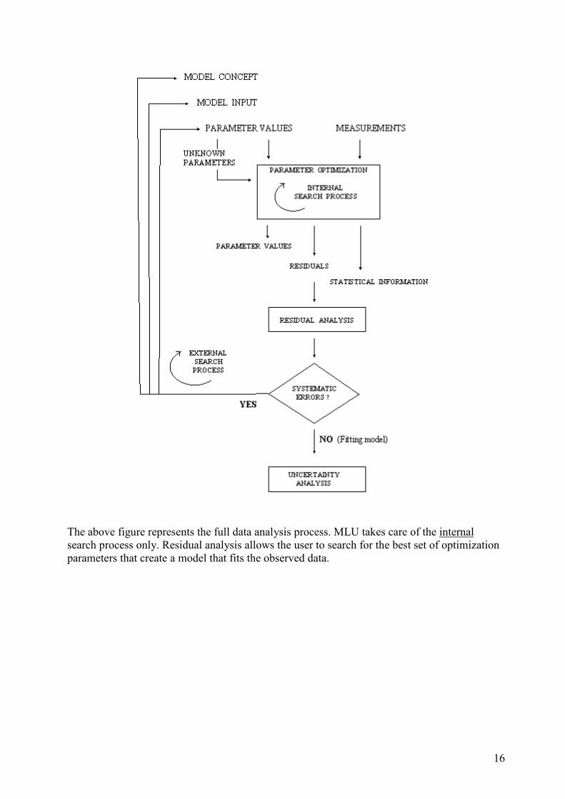
The above figure represents the full data analysis process. MLU takes care of the internal search process only. Residual analysis allows the user to search for the best set of optimization parameters that create a model that fits the observed data.
17
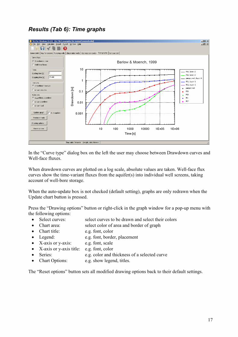
Results (Tab 6): Time graphs
In the “Curve type” dialog box on the left the user may choose between Drawdown curves and Well-face fluxes. When drawdown curves are plotted on a log scale, absolute values are taken. Well-face flux curves show the time-variant fluxes from the aquifer(s) into individual well screens, taking account of well-bore storage. When the auto-update box is not checked (default setting), graphs are only redrawn when the Update chart button is pressed. Press the “Drawing options” button or right-click in the graph window for a pop-up menu with the following options:
• Select curves: select curves to be drawn and select their colors
• Chart area: select color of area and border of graph
• Chart title: e.g. font, color
• Legend: e.g. font, border, placement
• X-axis or y-axis: e.g. font, scale
• X-axis or y-axis title: e.g. font, color
• Series: e.g. color and thickness of a selected curve
• Chart Options: e.g. show legend, titles. The “Reset options” button sets all modified drawing options back to their default settings.
18
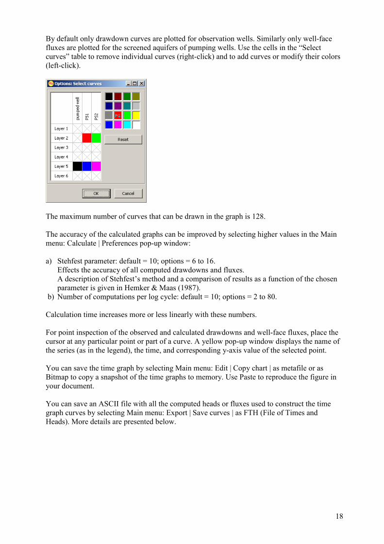
By default only drawdown curves are plotted for observation wells. Similarly only well-face fluxes are plotted for the screened aquifers of pumping wells. Use the cells in the “Select curves” table to remove individual curves (right-click) and to add curves or modify their colors (left-click).
The maximum number of curves that can be drawn in the graph is 128. The accuracy of the calculated graphs can be improved by selecting higher values in the Main menu: Calculate | Preferences pop-up window: a) Stehfest parameter: default = 10; options = 6 to 16. Effects the accuracy of all computed drawdowns and fluxes. A description of Stehfest’s method and a comparison of results as a function of the chosen parameter is given in Hemker & Maas (1987). b) Number of computations per log cycle: default = 10; options = 2 to 80. Calculation time increases more or less linearly with these numbers. For point inspection of the observed and calculated drawdowns and well-face fluxes, place the cursor at any particular point or part of a curve. A yellow pop-up window displays the name of the series (as in the legend), the time, and corresponding y-axis value of the selected point. You can save the time graph by selecting Main menu: Edit | Copy chart | as metafile or as Bitmap to copy a snapshot of the time graphs to memory. Use Paste to reproduce the figure in your document. You can save an ASCII file with all the computed heads or fluxes used to construct the time graph curves by selecting Main menu: Export | Save curves | as FTH (File of Times and Heads). More details are presented below.
19
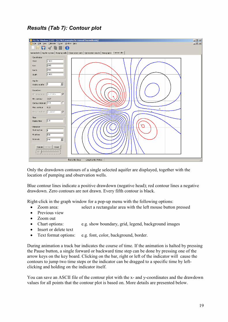
Results (Tab 7): Contour plot
Only the drawdown contours of a single selected aquifer are displayed, together with the location of pumping and observation wells. Blue contour lines indicate a positive drawdown (negative head); red contour lines a negative drawdown. Zero contours are not drawn. Every fifth contour is black. Right-click in the graph window for a pop-up menu with the following options:
• Zoom area: select a rectangular area with the left mouse button pressed
• Previous view
• Zoom out
• Chart options: e.g. show boundary, grid, legend, background images
• Insert or delete text
• Text format options: e.g. font, color, background, border. During animation a track bar indicates the course of time. If the animation is halted by pressing the Pause button, a single forward or backward time step can be done by pressing one of the arrow keys on the key board. Clicking on the bar, right or left of the indicator will cause the contours to jump two time steps or the indicator can be dragged to a specific time by left-clicking and holding on the indicator itself. You can save an ASCII file of the contour plot with the x- and y-coordinates and the drawdown values for all points that the contour plot is based on. More details are presented below.
20
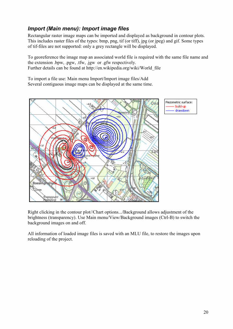
Import (Main menu): Import image files
Rectangular raster image maps can be imported and displayed as background in contour plots. This includes raster files of the types: bmp, png, tif (or tiff), jpg (or jpeg) and gif. Some types of tif-files are not supported: only a grey rectangle will be displayed. To georeference the image map an associated world file is required with the same file name and the extension .bpw, .pgw, .tfw, .jgw or .gfw respectively. Further details can be found at http://en.wikipedia.org/wiki/World_file To import a file use: Main menu Import/Import image files/Add Several contiguous image maps can be displayed at the same time.
Right clicking in the contour plot//Chart options.../Background allows adjustment of the brightness (transparency). Use Main menu/View/Background images (Ctrl-B) to switch the background images on and off. All information of loaded image files is saved with an MLU file, to restore the images upon reloading of the project.
21
Export (Main menu): Save curves as FTH
When a time graph is drawn, an ASCII file can be saved that contains all computed heads for all included observation wells, from the upper displayed aquifer down to the lowest displayed aquifer. FTH = File of Times and Heads. The file consists of the following parts. The first three lines contain: - The header. - The number of aquifers, the number of observation wells and “ 1”. - The actual numbers of these aquifers. The next four lines show a number for each well, the last part of their names, and their x- and y-coordinates. This is repeated for each aquifer. The main part of the file consist of a number of columns (up to 129); the first number on each line represents the time (days), while all the following numbers are calculated heads (or discharges) for all wells and for all aquifers. Times and discharges are saved in E-format, heads are saved in five decimals. FTH-files can be read by spreadsheets and by MicroFEM.
Export (Main menu): Save contours as XYZ
When a contour plot is drawn, a file can be saved that contains all computed drawdowns of the displayed contour plot. Each of the approximately 14000 lines contains three numbers: the x-coordinate, the y-coordinate and the computed drawdown. XYZ-files can be read by various GIS, CAD and similar mapping or graphics software (Surfer, Arcview).
22
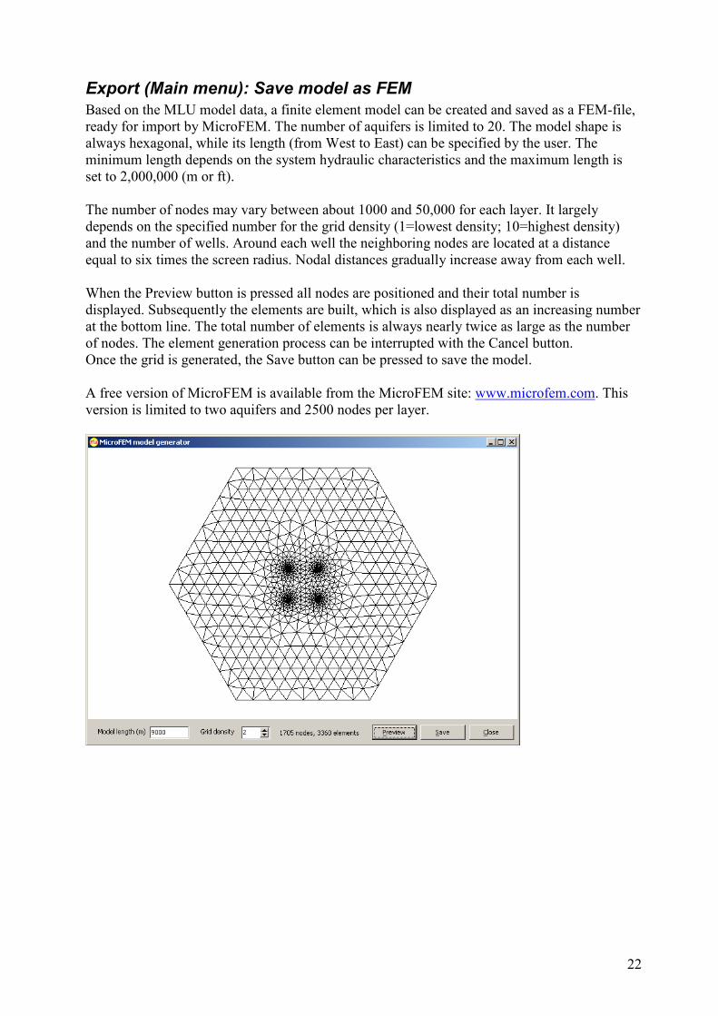
Export (Main menu): Save model as FEM
Based on the MLU model data, a finite element model can be created and saved as a FEM-file, ready for import by MicroFEM. The number of aquifers is limited to 20. The model shape is always hexagonal, while its length (from West to East) can be specified by the user. The minimum length depends on the system hydraulic characteristics and the maximum length is set to 2,000,000 (m or ft). The number of nodes may vary between about 1000 and 50,000 for each layer. It largely depends on the specified number for the grid density (1=lowest density; 10=highest density) and the number of wells. Around each well the neighboring nodes are located at a distance equal to six times the screen radius. Nodal distances gradually increase away from each well. When the Preview button is pressed all nodes are positioned and their total number is displayed. Subsequently the elements are built, which is also displayed as an increasing number at the bottom line. The total number of elements is always nearly twice as large as the number of nodes. The element generation process can be interrupted with the Cancel button. Once the grid is generated, the Save button can be pressed to save the model. A free version of MicroFEM is available from the MicroFEM site: www.microfem.com. This version is limited to two aquifers and 2500 nodes per layer.
23
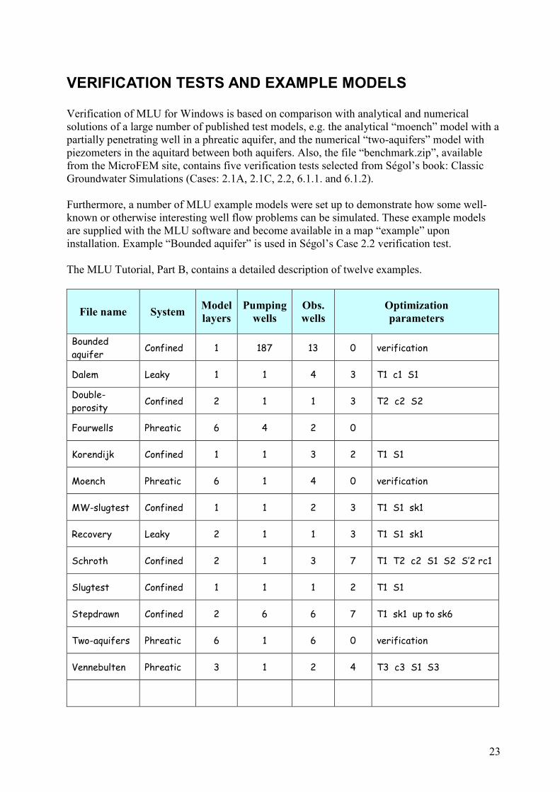
VERIFICATION TESTS AND EXAMPLE MODELS Verification of MLU for Windows is based on comparison with analytical and numerical solutions of a large number of published test models, e.g. the analytical “moench” model with a partially penetrating well in a phreatic aquifer, and the numerical “two-aquifers” model with piezometers in the aquitard between both aquifers. Also, the file “benchmark.zip”, available from the MicroFEM site, contains five verification tests selected from Ségol’s book: Classic Groundwater Simulations (Cases: 2.1A, 2.1C, 2.2, 6.1.1. and 6.1.2). Furthermore, a number of MLU example models were set up to demonstrate how some well-known or otherwise interesting well flow problems can be simulated. These example models are supplied with the MLU software and become available in a map “example” upon installation. Example “Bounded aquifer” is used in Ségol’s Case 2.2 verification test. The MLU Tutorial, Part B, contains a detailed description of twelve examples.
File name System Model
layers
Pumping
wells
Obs.
wells
Optimization
parameters
Bounded
aquifer Confined 1 187 13 0 verification
Dalem Leaky 1 1 4 3 T1 c1 S1
Double-
porosity Confined 2 1 1 3 T2 c2 S2
Fourwells Phreatic 6 4 2 0
Korendijk Confined 1 1 3 2 T1 S1
Moench Phreatic 6 1 4 0 verification
MW-slugtest Confined 1 1 2 3 T1 S1 sk1
Recovery Leaky 2 1 1 3 T1 S1 sk1
Schroth Confined 2 1 3 7 T1 T2 c2 S1 S2 S’2 rc1
Slugtest Confined 1 1 1 2 T1 S1
Stepdrawn Confined 2 6 6 7 T1 sk1 up to sk6
Two-aquifers Phreatic 6 1 6 0 verification
Vennebulten Phreatic 3 1 2 4 T3 c3 S1 S3
24
Main characteristics of the example models
bounded-aquifer.mlu
Ségol (1994) Classic Groundwater Simulations, page 49-51, Case 2.2, Alternative B Rectangular confined aquifer 9000 * 5000 m No-flow boundaries at South and West side; Fixed head boundaries at North and East side. Solution uses 11 * 17 - 1 = 186 image wells. See e.g. Kruseman & de Ridder (Chapter 6) for a discussion on the use of image wells to model well flow in bounded aquifers. Drawdowns are obtained along southern boundary for 3 times: 0.05, 0.15 and 2 days. Comparison with analytical and numerical results (see: “benchmark.zip”)
dalem.mlu
Kruseman & de Ridder (2000) p. 83-84 Leaky aquifer, 1 pumping well and 4 piezometers (51 observations) Graphical results: T=1800 m2/d; S=0.0017; c=450 d. Linear drawdown curve fitting: T=1676 m2/d; S=0.0018; c=328 d. Log drawdown curve fitting: T=1780 m2/d; S=0.0016; c=539 d.
double-porosity.mlu
Kruseman & de Ridder (2000) p. 258-261 (after Moench 1984) Modeled as a two-aquifer confined system. See e.g. Hemker & Maas (1987) for a short discussion on the similarity between layered and fissured formations. 72 observations in pumped well. Graphical solution: T=333 m2/d; S=0.0016. Linear drawdown curve fitting: T=334 m2/d; S=0.0032.
fourwells.mlu
Test example of a 4 wells square ATES (Aquifer thermal energy storage) configuration. Alternating two-wells discharging and two-wells injecting in a yearly cycle. Phreatic multi-aquifer system: 6 model layers. Wells screened in 3rd aquifer = 3 model layers + 2 zero-thickness resistance layers. Contour plot animation verifies crosswise symmetric drawdown - build-up cone patterns.
moench.mlu
Moench (1997) Flow to a well of finite diameter in a homogeneous, anisotropic water table aquifer: Water Resources Research, v. 33, no. 6, p. 1397–1407. See also Paul M. Barlow and Allen F. Moench, 1999, Water-Resources Investigations Report 99-4225, WTAQ Sample Problem 2. http://ma.water.usgs.gov/publications/WRIR_99-4225/index.htm Water-table aquifer. Partially penetrating pumping well of finite diameter. 6-Layer MLU model simulates full 3D-analytical solution.
25
1 10 100 1000 10000 1E+05 1E+06 1E+07 1E+08 1E+09
1E-04
0.001
0.01
0.1
1
10 PS1, layer: 2
PS2, layer: 2
pumped well, layer: 5
PS1, layer: 5
PS2, layer: 5
pumped well
PS1
PS2
PD1
PD2
Drawdown - time
Time [s]
Dra
wd
ow
n [m
]
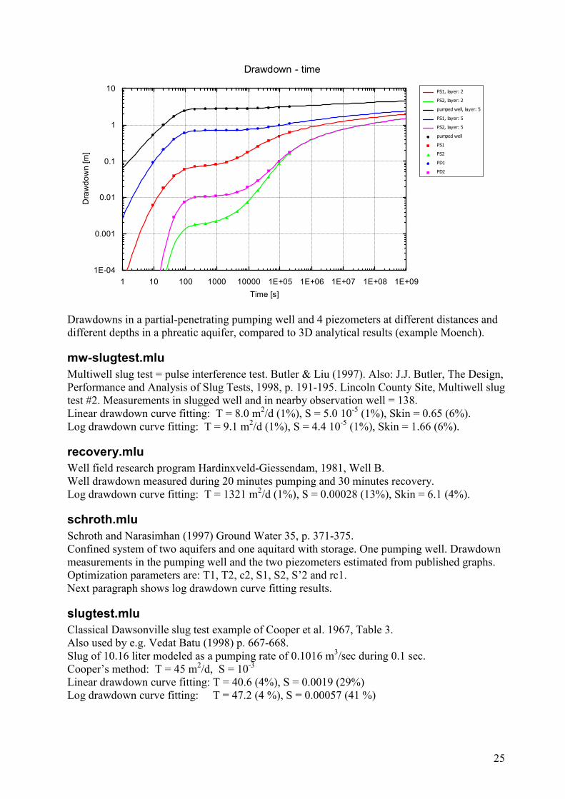
Drawdowns in a partial-penetrating pumping well and 4 piezometers at different distances and different depths in a phreatic aquifer, compared to 3D analytical results (example Moench).
mw-slugtest.mlu
Multiwell slug test = pulse interference test. Butler & Liu (1997). Also: J.J. Butler, The Design, Performance and Analysis of Slug Tests, 1998, p. 191-195. Lincoln County Site, Multiwell slug test #2. Measurements in slugged well and in nearby observation well = 138. Linear drawdown curve fitting: T = 8.0 m2/d (1%), S = 5.0 10-5 (1%), Skin = 0.65 (6%). Log drawdown curve fitting: T = 9.1 m2/d (1%), S = 4.4 10-5 (1%), Skin = 1.66 (6%).
recovery.mlu
Well field research program Hardinxveld-Giessendam, 1981, Well B. Well drawdown measured during 20 minutes pumping and 30 minutes recovery. Log drawdown curve fitting: T = 1321 m2/d (1%), S = 0.00028 (13%), Skin = 6.1 (4%).
schroth.mlu
Schroth and Narasimhan (1997) Ground Water 35, p. 371-375. Confined system of two aquifers and one aquitard with storage. One pumping well. Drawdown measurements in the pumping well and the two piezometers estimated from published graphs. Optimization parameters are: T1, T2, c2, S1, S2, S’2 and rc1. Next paragraph shows log drawdown curve fitting results.
slugtest.mlu
Classical Dawsonville slug test example of Cooper et al. 1967, Table 3. Also used by e.g. Vedat Batu (1998) p. 667-668. Slug of 10.16 liter modeled as a pumping rate of 0.1016 m3/sec during 0.1 sec. Cooper’s method: T = 45 m2/d, S = 10-3 Linear drawdown curve fitting: T = 40.6 (4%), S = 0.0019 (29%) Log drawdown curve fitting: T = 47.2 (4 %), S = 0.00057 (41 %)
26
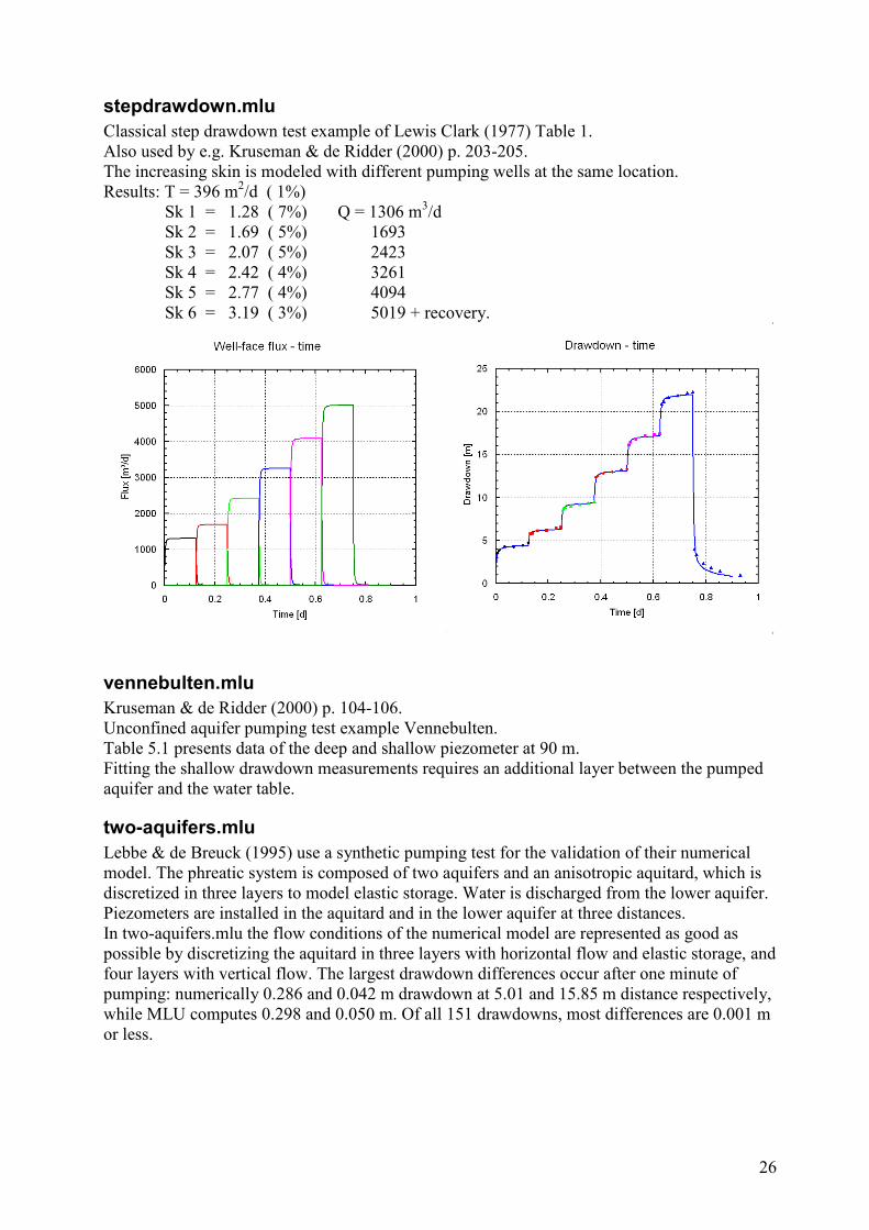
stepdrawdown.mlu
Classical step drawdown test example of Lewis Clark (1977) Table 1. Also used by e.g. Kruseman & de Ridder (2000) p. 203-205. The increasing skin is modeled with different pumping wells at the same location. Results: T = 396 m2/d ( 1%) Sk 1 = 1.28 ( 7%) Q = 1306 m3/d Sk 2 = 1.69 ( 5%) 1693 Sk 3 = 2.07 ( 5%) 2423 Sk 4 = 2.42 ( 4%) 3261 Sk 5 = 2.77 ( 4%) 4094 Sk 6 = 3.19 ( 3%) 5019 + recovery.
vennebulten.mlu
Kruseman & de Ridder (2000) p. 104-106. Unconfined aquifer pumping test example Vennebulten. Table 5.1 presents data of the deep and shallow piezometer at 90 m. Fitting the shallow drawdown measurements requires an additional layer between the pumped aquifer and the water table.
two-aquifers.mlu
Lebbe & de Breuck (1995) use a synthetic pumping test for the validation of their numerical model. The phreatic system is composed of two aquifers and an anisotropic aquitard, which is discretized in three layers to model elastic storage. Water is discharged from the lower aquifer. Piezometers are installed in the aquitard and in the lower aquifer at three distances. In two-aquifers.mlu the flow conditions of the numerical model are represented as good as possible by discretizing the aquitard in three layers with horizontal flow and elastic storage, and four layers with vertical flow. The largest drawdown differences occur after one minute of pumping: numerically 0.286 and 0.042 m drawdown at 5.01 and 15.85 m distance respectively, while MLU computes 0.298 and 0.050 m. Of all 151 drawdowns, most differences are 0.001 m or less.
27
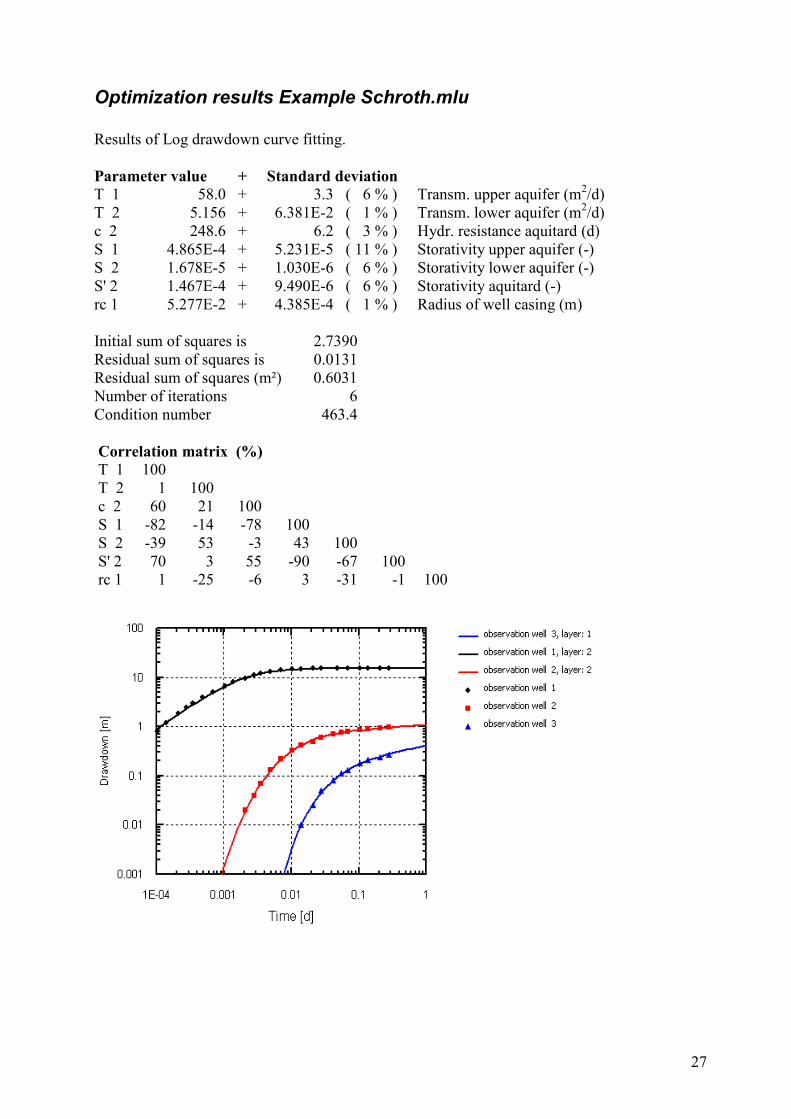
Optimization results Example Schroth.mlu
Results of Log drawdown curve fitting.
Parameter value + Standard deviation
T 1 58.0 + 3.3 ( 6 % ) Transm. upper aquifer (m2/d) T 2 5.156 + 6.381E-2 ( 1 % ) Transm. lower aquifer (m2/d) c 2 248.6 + 6.2 ( 3 % ) Hydr. resistance aquitard (d) S 1 4.865E-4 + 5.231E-5 ( 11 % ) Storativity upper aquifer (-) S 2 1.678E-5 + 1.030E-6 ( 6 % ) Storativity lower aquifer (-) S' 2 1.467E-4 + 9.490E-6 ( 6 % ) Storativity aquitard (-) rc 1 5.277E-2 + 4.385E-4 ( 1 % ) Radius of well casing (m) Initial sum of squares is 2.7390 Residual sum of squares is 0.0131 Residual sum of squares (m²) 0.6031 Number of iterations 6 Condition number 463.4
Correlation matrix (%)
T 1 100 T 2 1 100 c 2 60 21 100 S 1 -82 -14 -78 100 S 2 -39 53 -3 43 100 S' 2 70 3 55 -90 -67 100 rc 1 1 -25 -6 3 -31 -1 100
28
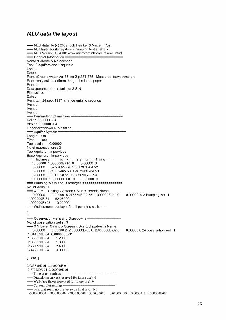
MLU data file layout
=== MLU data file (c) 2009 Kick Hemker & Vincent Post === Multilayer aquifer system - Pumping test analysis === MLU Version 1.54.00: www.microfem.nl/products/mlu.html === General Information ============================= Name :Schroth & Narasimhan Test :2 aquifers and 1 aquitard Loc. : Date : Rem. :Ground water Vol 35. no 2 p.371-375 Measured drawdowns are Rem. :only estimatedfrom the graphs in the paper Rem. : Data :parameters = results of S & N File :schroth Date : Rem. :cjh 24 sept 1997 change units to seconds Rem. : Rem. : Rem. : === Parameter Optimization ========================== Rel.: 1.000000E-04 Abs.: 1.000000E-04 Linear drawdown curve fitting === Aquifer System ================================== Length : m Time : sec Top level : 0.00000 No of (sub)aquifers : 2 Top Aquitard : Impervious Base Aquitard : Impervious === Thickness === T|c = x === S|S' = x === Name ==== 46.00000 1.000000E+10 0 0.00000 0 3.00000 57.97095 49 4.861797E-04 52 3.00000 248.62465 50 1.467240E-04 53 3.00000 5.15558 51 1.677179E-05 54 100.00000 1.000000E+10 0 0.00000 0 === Pumping Wells and Discharges ==================== No. of wells : 1 === X Y Casing x Screen x Skin x Periods Name 0.00000 0.00000 5.276889E-02 55 1.000000E-01 0 0.00000 0 2 Pumping well 1 1.000000E-31 82.08000 1.000000E+08 0.00000 === Well screens per layer for all pumping wells ==== . 1 === Observation wells and Drawdowns ================= No. of observation wells : 3 === X Y Layer Casing x Screen x Skin x drawdowns Name 0.00000 0.00000 2 2.000000E-02 0 2.000000E-02 0 0.00000 0 24 observation well 1 1.041670E-04 8.000000E-01 1.388890E-04 1.20000 2.083330E-04 1.80000 2.777780E-04 2.40000 3.472220E-04 3.00000 [Jetc. ] 2.083330E-01 2.400000E-01 2.777780E-01 2.700000E-01 === Time graph settings ============================= === Drawdown curves (reserved for future use): 0 === Well-face fluxes (reserved for future use): 0 === Contour plot settings =========================== === west east south north start steps final layer del -5000.00000 5000.00000 -3000.00000 3000.00000 0.00000 50 10.00000 1 1.000000E-02
29
References
The techniques used in MLU are based on the theory as described in the following publications:
Hemker, C.J. (1984) Steady groundwater flow in leaky multiple-aquifer systems. Journal of Hydrology, 72: 355-374. Hemker, C.J. (1985) Transient well flow in leaky multiple-aquifer systems. Journal of Hydrology, 81: 111-126. Hemker, C.J. (1985) A General Purpose Microcomputer Aquifer Test Evaluation Technique. Ground Water 23: 247-253. Hemker, C.J. and C. Maas (1987) Unsteady flow to wells in layered and fissured aquifer systems. Journal of Hydrology, 90: 231-249. Hemker, C.J. and C. Maas (1994) Comment on "Multilayered leaky aquifer systems, 1, Pumping well solutions" by A.H.-D Cheng and O.K. Morohunfola Water Resources Research, Vol. 30, No. 11, p. 3229-3230. Hemker, C.J. (1999a) Transient well flow in vertically heterogeneous aquifers. Journal of Hydrology, 225: 1-18. Hemker, C.J. (1999b) Transient well flow in layered aquifer systems: the uniform well-face drawdown solution. Journal of Hydrology, 225: 19-44. You may contact the author [email protected] for a PDF of the above publications. References made in the description of the example models:
Barlow, P.M. and A.F. Moench (1999) WTAQ - A computer program for calculating drawdowns and estimating hydraulic properties for confined and water-table aquifers, U.S. Geol. Survey Water-Resources Investigations Report 99-4225, 74 pp. Batu, Vedat (1998) Aquifer Hydraulics: A Comprehensive Guide to Hydrogeologic Data Analysis. John Wiley & Sons, Inc. 727 pp. Butler, J.J.Jr. (1998) The Design, Performance, and Analysis of Slug Tests, Lewis Publishers, Boca Raton, 252 pp. Butler, J.J.Jr. and W.Z. Liu (1997) Analysis of 1991-1992 slug test in the Dakota aquifer of central and western Kansas, Kans. Geol. Surv.. Open-File Rep. 93-1c. Clark, L. (1977) The analysis and planning of step drawdown tests. Quart. J. Engng Geol. 10: 125-143. Cooper, H.H, J.D. Bredehoeft and S.S. Papadopoulos (1967) Response of a finite-diameter well to an instantaneous charge of water. Water Resour. Res. 3: 263-269. Kruseman, G.P. and N.A. de Ridder (2000) Analysis and evaluation of pumping test data. ILRI publication 47, Wageningen, The Netherlands, 377 pp. https://www.hydrology.nl/images/docs/dutch/key/Kruseman_and_De_Ridder_2000.pdf Lebbe, L. and W. De Breuck (1995) Validation of an inverse numerical model for interpretation of pumping tests and the study of factors influencing accuracy of results. Journal of Hydrology, 172: 61-85. Moench, A.F. (1984) Double-porosity models for a fissured groundwater reservoir with fracture skin, Water Resour. Res. 20: 831–846. Moench, A.F. (1997) Flow to a well of finite diameter in a homogeneous, anisotropic water table aquifer, Water Resour. Research, 33 (6) 1397-1407. Schroth, B, and T. N. Narasimhan (1997) Application of a numerical model in the interpretation of a leaky aquifer test. Ground water 35: 371-375. Ségol, G. (1994) Classic groundwater simulations: Proving and improving numerical models. Prentice-Hall. 531 pp.
30
License agreement
MLU for Windows © 2008-2018 by C.J. Hemker & V.E.A. Post, Amsterdam Hemker & Post retain the ownership of all copies of the MLU software. A copy is licensed to the purchaser for use under the following conditions: 1. Copyright Notice This software is protected by both Dutch copyright law and international treaty provisions. Hemker & Post authorizes the purchaser to make archive copies of the software for the purpose of backing up the MLU software. The purchaser of a license is also allowed to make copies of the software and use his backups of the software on more than one of his own machines, on the strict condition that these backups are only used within the city of the purchaser's office or within the department of the university concerned. Specifically the purchaser may not rent, sub-license, or lease the software or documentation; alter, modify, or adapt the software or documentation, including, but not limited to translating, de-compiling, disassembling, or creating derivative works without the prior written consent of Hemker & Post. 2. Warranty The MLU software has been used and tested since 1987 (DOS version). No software is completely error free, however. Should you encounter a bug, Hemker & Post will immediately work on it and supply you with a corrected version at no charge. This warranty shall be limited to replacement and shall not encompass any other damages, including, but not limited to, loss of profit, and special, incidental, consequential, or other similar claims. 3. Disclaimer Except as specifically provided above, neither the developer of this software nor any person or organization acting on behalf of him gives any warranty, express or implied, with respect to this software. In no event will Hemker & Post assume any liability with respect to the use, or misuse, of this software, or the interpretation, or misinterpretation, of any results obtained from this software, or for direct, indirect, special, incidental, or consequential damages resulting from the use of this software. Specifically Hemker & Post is not responsible for any costs including, but not limited to, those incurred as a result of lost profits or revenue, loss of use of the computer program, loss of data, the costs of recovering such programs or data, the costs of any substitute program, claims by third parties, or for other similar costs. In no case shall the liability of Hemker & Post exceed the amount of the license fee.