MIXED FINITE ELEMENT METHODS FOR ELLIPTIC PROBLEMS*

DOUGLAS N. ARNOLD†

Abstract. This paper treats the basic ideas of mixed finite element methods at an introductory level.

Although the viewpoint presented is that of a mathematician, the paper is aimed at practitioners and themathematical prerequisites are kept to a minimum. A classification of variational principles and of the

corresponding weak formulations and Galerkin methods—displacement, equilibrium, and mixed—is givenand illustrated through four significant examples. The advantages and disadvantages of mixed methods

are discussed. The concepts of convergence, approximability, and stability and their interrelations are

developed, and a resume is given of the stability theory which governs the performance of mixed methods.The paper concludes with a survey of techniques that have been developed for the construction of stable

mixed methods and numerous examples of such methods.

Key words. mixed method, finite element, variational principle

1. Introduction. The term mixed method was first used in the 1960’s to describefinite element methods in which both stress and displacement fields are approximated asprimary variables. We begin with the most classical example, the system of linear elasticity.

The equations of linear elasticity consist of the constitutive equation

AS = E(u) in Ω

and the equilibrium equationdivS = f in Ω.

Here Ω denotes the region in three dimensional space, R3, occupied by the elastic body,u : Ω → R

3 denotes the displacement field, E(u) denotes the corresponding infinitesimalstrain tensor, (i.e., the symmetric part of the gradient of u, εij(u) = (ui,j + uj,i)/2)), fdenotes the imposed volume load, and S : Ω→ R

3×3s (the space of symmetric 3×3 tensors)

denotes the stress field. The divergence of S, divS, is applied to each row of S, so that(divS)i =

∑j sij,j . The material properties are determined by the compliance tensor A

which is a positive definite symmetric operator from R3×3s to itself,1 possibly depending

on the point x ∈ Ω. The constitutive equations can equally well be written as

S = CE(u) in Ω

*This work was supported by NSF grant DMS-89-02433.†Department of Mathematics, The Pennsylvania State University, University Park, Pennsylvania

16827.1This means that the action of A can be written as (AS)ij =

∑kl aijklskl with the components

aijkl satisfying the usual major symmetries aijkl = aklij , minor symmetries aijkl = ajikl, and positivity

condition∑ijkl aijklsijskl ≥ γ

∑ij s

2ij , for all S, where γ > 0.

Typeset by AMS-TEX

where the elasticity tensor C : R3×3s → R

3×3s is the inverse of A. This example also serves

to illustrate our font conventions: vector quantities are notated in boldface, second ordertensors are in script, and fourth order tensors are sans serif.

To determine a unique solution, we supplement the elasticity equations by the boundaryconditions

u |Γd = gd and Sn |Γt = gt

where Γd and Γt are complementary parts of ∂Ω and gd and gt give the displacementsand tractions prescribed on Γd and Γt respectively.

Mixed methods for the elasticity problem are mostly based on the following mixedvariational principle which is a form of the Hellinger–Reissner principle:

The solution (S,u) of the elasticity problem can be characterized as theunique critical point of the functional

L(T , v) =∫

Ω

(12

A T :T + div T · v− f · v)−∫

Γd

gd · (T n)

over the space of all symmetric tensorfields T satisfying the traction bound-ary condition T n |Γt = gt, and all vectorfields v.

Indeed, if we set the first variation of L with respect to T equal to zero, we get the equation∫Ω

(AS :T + div T · u) =∫

Γd

gd · (T n)

for all T for which T n vanishes on Γt. Integrating by parts, we obtain the constitutiveequation and displacement boundary condition. Taking the variation of L with respect tov leads immediately to the equilibrium equation. Note that in the form of the Hellinger–Reissner principle presented, the traction boundary condition is essential—it is imposeda priori on the space where the stress tensor is sought—while the displacement boundarycondition arises naturally from the variational principle.

To make the variational principle precise, we must state over what space of functionsT and v are to vary. The appropriate choice for T is the subspace of H(div) (symmetrictensorfields which are square integrable and have square integrable divergence) of fieldssatisfying the traction boundary condition, and for v the space L2 of all square integrablevectorfields. The reader who is uncomfortable with these function spaces need not beconcerned: suffice it to say that they are chosen in a fairly natural way so that the integralsinvolved in the definition of L make sense.

A key point, which is characteristic of mixed variational principles, is that the pair(S,u) is not an extreme point of the Hellinger–Reissner functional. It is a saddle point.In fact

L(S, v) ≤ L(S,u) ≤ L(T ,u)

2

for all T ∈ H(div) satisfying T n |Γt = gt and all u ∈ L2. It follows from this saddle pointcondition that

(1) supv∈L2

infT ∈H(div)T n |Γt=gt

L(T , v) = L(S,u) and infT ∈H(div)T n |Γt=gt

supv∈L2

L(T , v) = L(S,u).

Now, because u satisfies the constitutive equation, E(u) is square integrable. It follows(from Korn’s inequality) that the gradient of u is square integrable, i.e., u ∈ H1. Let usset, for any v ∈ L2,

E(v) = − infT ∈H(div)T n |Γt=gt

L(T , v).

Then E(u) = −L(S,u) and we have from (1) that

−E(u) = supv∈L2

−E(v),

and, a fortiori,−E(u) = sup

v∈H1−E(v)

or

(2) E(u) = infv∈H1

E(v),

i.e., the displacement field u is characterized as the minimizer of the functional E over H1.We shall show in a moment that for any v ∈ H1

(3) E(v) = ∫ ( 1

2 C E(v) :E(v) + f · v)−∫

Γtgt · v, if v |Γd = gd

∞, otherwise.

This permits us to interpret (2) as the following variational priniciple, which is nothingbut the usual prinicipal of minimal potential energy energy.

The displacement field u solving the elasticity problem minimizes the func-tional ∫

Ω

(12

C E(v) :E(v) + f · v)−∫

Γt

gt · v

over the space of all vectorfields satsifying the displacement boundary con-ditions.

Thus, starting from the Hellinger–Reissner mixed principle, we have derived the standarddisplacement variational principle. Note that for the latter the displacement boundarycondition is essential, and the traction condition natural.

3

To verify (3) we integrate by parts to get

L(T , v) =∫

Ω

(12

A T :T − T : E(v)− f · v)

+∫

Γt

gt · v+∫

Γd

(v− gd) · (T n).

Now if v − gd doesn’t vanish on Γd, then we may take T such that T n is an arbitrarilylarge negative multiple of this quantity on Γd, and we can arrange as well that T decayquickly away from ∂Ω so that its L2 norm is arbitrarily small. It follows that L(T , v) canbe made negative with arbitrarily large magnitude by appropriate choice of T . Thus, ifv |Γd 6= gd, then E(v) =∞. On the other hand, if v |Γd = gd, then

L(T , v) =∫

Ω

(12

A T :T − T : E(v)− f · v)

+∫

Γt

gt · v.

This quantity is clearly minimal when A T = E(v), i.e, when T = C E(v), and in this case

L(T , v) =∫

Ω

(−1

2C E(v) : E(v)− f · v

)+∫

Γt

gt · v,

as claimed.

We have seen how the stress field can be eliminated from the mixed variational princi-ple, leaving a variational characterization of the displacement. In a similar (simpler) waywe can eliminate the displacement and obtain the following variational characterizationof the stress: of all tensorfields which satisfy the equilibrium equation and the tractionboundary conditions, S minimizes the complementary energy functional

Ec(T ) =∫

Ω

12

A T : T −∫

Γd

gd · (T n).

These three basic variational principles for linear elasticity are summarized in Table 1. Foreach of these variational principles, the critical point is determined by the vanishing of thefirst variation, which leads to a weakly formulated boundary value problem. The weakformulations corresponding to our three variational principles are given in Table 2.

Each of the three variational principles may be discretized by seeking a critical pointof the relevant functional over a finite dimensional subspace (presumably of finite elementtype) of the admissable trial functions. Equivalently, in the weak formulations we cansubstitute the function spaces (H1,H(div), and L2) with finite dimensional subspaces. Theresulting discretization methods are termed Galerkin methods. For the primal principlethe resulting Galerkin methods are termed displacement methods. For the dual principlesuch methods are commonly referred to as equilibrium methods. For the mixed variationalprinciple we obtain mixed methods. In all three cases, the determination of the discretesolution ultimately reduces to the solution of a finite system of algebraic equations.

4

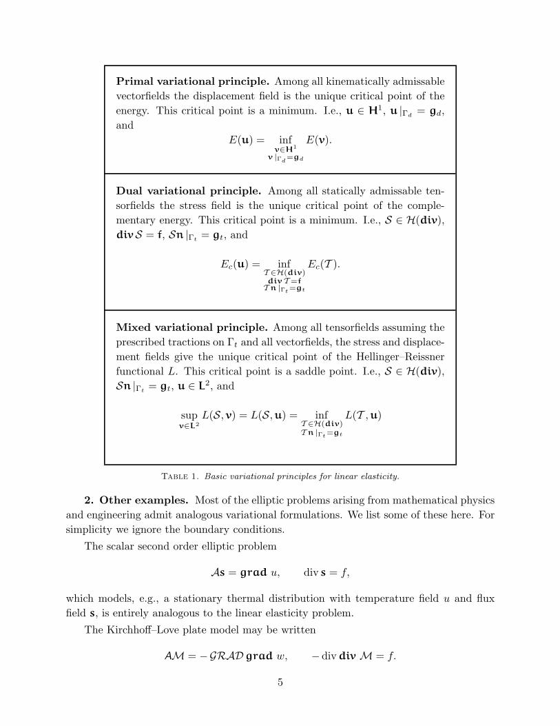
Primal variational principle. Among all kinematically admissablevectorfields the displacement field is the unique critical point of theenergy. This critical point is a minimum. I.e., u ∈ H1, u |Γd = gd,and

E(u) = infv∈H1

v |Γd=gd

E(v).

Dual variational principle. Among all statically admissable ten-sorfields the stress field is the unique critical point of the comple-mentary energy. This critical point is a minimum. I.e., S ∈ H(div),divS = f, Sn |Γt = gt, and

Ec(u) = infT ∈H(div)div T=fT n |Γt=gt

Ec(T ).

Mixed variational principle. Among all tensorfields assuming theprescribed tractions on Γt and all vectorfields, the stress and displace-ment fields give the unique critical point of the Hellinger–Reissnerfunctional L. This critical point is a saddle point. I.e., S ∈ H(div),Sn |Γt = gt, u ∈ L2, and

supv∈L2

L(S, v) = L(S,u) = infT ∈H(div)T n |Γt=gt

L(T ,u)

Table 1. Basic variational principles for linear elasticity.

2. Other examples. Most of the elliptic problems arising from mathematical physicsand engineering admit analogous variational formulations. We list some of these here. Forsimplicity we ignore the boundary conditions.

The scalar second order elliptic problem

As = grad u, div s = f,

which models, e.g., a stationary thermal distribution with temperature field u and fluxfield s, is entirely analogous to the linear elasticity problem.

The Kirchhoff–Love plate model may be written

AM = −GRADgrad w, −divdivM = f.

5

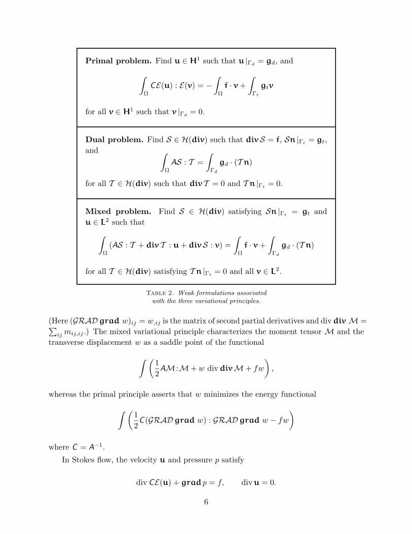
Primal problem. Find u ∈ H1 such that u |Γd = gd, and∫Ω

CE(u) : E(v) = −∫

Ω

f · v+∫

Γt

gtv

for all v ∈ H1 such that v |Γd = 0.

Dual problem. Find S ∈ H(div) such that divS = f, Sn |Γt = gt,and ∫

Ω

AS : T =∫

Γd

gd · (T n)

for all T ∈ H(div) such that div T = 0 and T n |Γt = 0.

Mixed problem. Find S ∈ H(div) satisfying Sn |Γt = gt andu ∈ L2 such that∫

Ω

(AS : T + div T : u+ divS : v) =∫

Ω

f · v+∫

Γd

gd · (T n)

for all T ∈ H(div) satisfying T n |Γt = 0 and all v ∈ L2.

Table 2. Weak formulations associated

with the three variational principles.

(Here (GRADgrad w)ij = w,ij is the matrix of second partial derivatives and divdivM =∑ijmij,ij .) The mixed variational principle characterizes the moment tensor M and the

transverse displacement w as a saddle point of the functional∫ (12

AM :M+ w divdivM+ fw

),

whereas the primal principle asserts that w minimizes the energy functional∫ (12

C (GRADgrad w) : GRADgrad w − fw)

where C = A−1.

In Stokes flow, the velocity u and pressure p satisfy

div CE(u) + grad p = f, divu = 0.

6

Together they are a saddle point of the the functional∫ (12

CE(u) :E(u) + pdivu+ fu

).

For Stokes problems the primal variational principle, which characterizes the pressureindependently of the velocity, is rarely used. This is because it involves the inversion of thedifferential operator div CE(·), which is rarely practical. On the other hand, equilibriummethods, based on the dual principle that u minimize∫ (

12

CE(u) :E(u) + fu

)over divergence-free fields, are occasionally used.

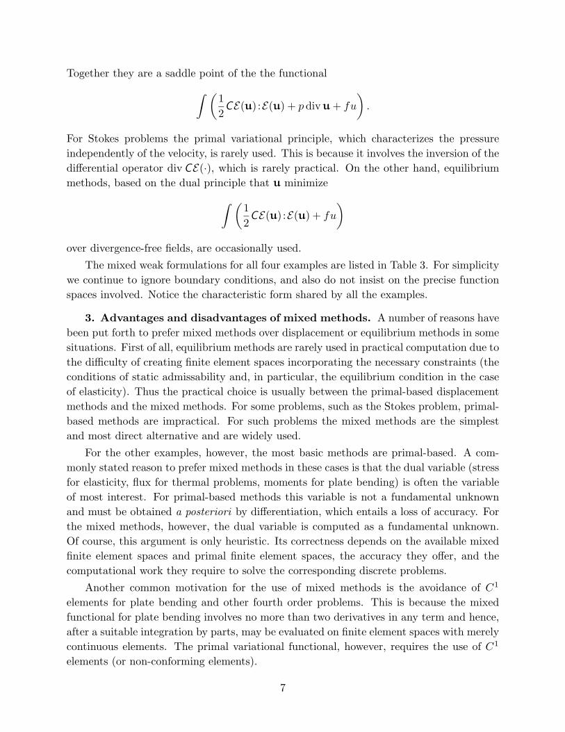
The mixed weak formulations for all four examples are listed in Table 3. For simplicitywe continue to ignore boundary conditions, and also do not insist on the precise functionspaces involved. Notice the characteristic form shared by all the examples.

3. Advantages and disadvantages of mixed methods. A number of reasons havebeen put forth to prefer mixed methods over displacement or equilibrium methods in somesituations. First of all, equilibrium methods are rarely used in practical computation due tothe difficulty of creating finite element spaces incorporating the necessary constraints (theconditions of static admissability and, in particular, the equilibrium condition in the caseof elasticity). Thus the practical choice is usually between the primal-based displacementmethods and the mixed methods. For some problems, such as the Stokes problem, primal-based methods are impractical. For such problems the mixed methods are the simplestand most direct alternative and are widely used.

For the other examples, however, the most basic methods are primal-based. A com-monly stated reason to prefer mixed methods in these cases is that the dual variable (stressfor elasticity, flux for thermal problems, moments for plate bending) is often the variableof most interest. For primal-based methods this variable is not a fundamental unknownand must be obtained a posteriori by differentiation, which entails a loss of accuracy. Forthe mixed methods, however, the dual variable is computed as a fundamental unknown.Of course, this argument is only heuristic. Its correctness depends on the available mixedfinite element spaces and primal finite element spaces, the accuracy they offer, and thecomputational work they require to solve the corresponding discrete problems.

Another common motivation for the use of mixed methods is the avoidance of C1

elements for plate bending and other fourth order problems. This is because the mixedfunctional for plate bending involves no more than two derivatives in any term and hence,after a suitable integration by parts, may be evaluated on finite element spaces with merelycontinuous elements. The primal variational functional, however, requires the use of C1

elements (or non-conforming elements).

7

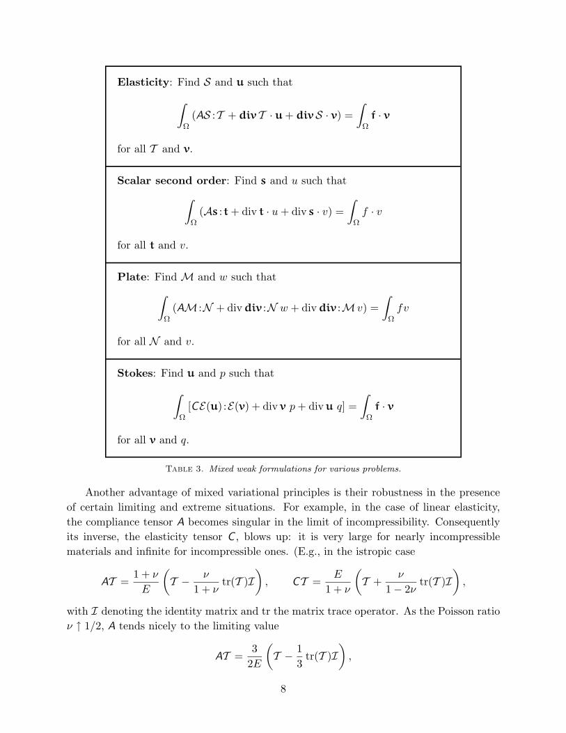
Elasticity: Find S and u such that∫Ω

(AS :T + div T · u+ divS · v) =∫

Ω

f · v

for all T and v.

Scalar second order: Find s and u such that∫Ω

(As :t+ div t · u+ div s · v) =∫

Ω

f · v

for all t and v.

Plate: Find M and w such that∫Ω

(AM :N + divdiv :N w + divdiv :M v) =∫

Ω

fv

for all N and v.

Stokes: Find u and p such that∫Ω

[CE(u) :E(v) + div v p+ divu q] =∫

Ω

f · v

for all v and q.

Table 3. Mixed weak formulations for various problems.

Another advantage of mixed variational principles is their robustness in the presenceof certain limiting and extreme situations. For example, in the case of linear elasticity,the compliance tensor A becomes singular in the limit of incompressibility. Consequentlyits inverse, the elasticity tensor C , blows up: it is very large for nearly incompressiblematerials and infinite for incompressible ones. (E.g., in the istropic case

AT =1 + ν

E

(T − ν

1 + νtr(T )I

), CT =

E

1 + ν

(T +

ν

1− 2νtr(T )I

),

with I denoting the identity matrix and tr the matrix trace operator. As the Poisson ratioν ↑ 1/2, A tends nicely to the limiting value

AT =3

2E

(T − 1

3tr(T )I

),

8

but C blows up.) A analogous situation holds for the Reissner–Mindlin plate model wherethe robustness is with respect to the plate thickness. Robustness properties of mixedmethods have also been reported in other situations, as well. That is, mixed methods havebeen observed to perform significantly better than closely related displacement methodsin particular applications that involve some extreme or limiting behavior. For example,Ewing, Wheeler, and others have reported superior computations of pressure (which sat-isfies a scalar second order elliptic problem arising from Darcy’s law) via mixed methodswhen simulating the miscible displacement of oil from a porous media [12], [13]. Mariniand Savini [20] have reported improved results in semiconductor device modelling throughthe use of mixed methods. In each case, the mixed methods seem to be exhibiting greaterrobustness with respect to the roughness of the coefficients of the equations. (In bothproblems there is a sharply defined front across which the coefficients change rapidly.)

In addition to the situations in which mixed methods are used explicitly, there are anumber of methods which have been proposed in the literature which, while resemblingdisplacement methods, can be shown to be equivalent to mixed methods. Such methods arecalled generalized displacement methods since they lead to discrete systems involving onlydegrees of freedom associated to the primal variable. However the discrete system differsfrom what would be obtained by straightforward discretization of the primal variationalprinciple. The best known examples are the reduced and selective integration methods inwhich all or some of the terms of the primal energy functional are intentionally integratedwith low accuracy. This apparently paradoxical procedure of reducing the integrationaccuracy in order to increase the solution accuracy was poorly understood and quite con-troversial when first introduced. In almost every case where it is successful, however, it canbe shown that such a method is equivalent to a rather natural mixed method with exact,or at least accurate, integration [19]. In a number of cases the theory of mixed methodscan be applied to provide a complete understanding and justification of reduced integra-tion procedures. (Cf. [1] where the theory of mixed methods is used to give a completeanalysis of reduced integration and standard displacement methods for the Timoshenkobeam problem and [18] where some reduced integration methods for the Stokes problemand Reissner-Mindlin plate are analyzed as mixed methods.) A similar situation holdsfor other generalized displacement methods, such as ones involving harmonic averaging ofrough coefficients [6] and interpolation [8] in the computation of the stiffness matrix. Inaddition a number of non-conforming displacement methods can be viewed, and best ana-lyzed, as mixed methods [2]. In our view, this constitutes one of the most important rolesof the theory of mixed methods: it provides tools to design and analyze high performancegeneralized displacement methods.

There are also obvious disadvantages to mixed methods in comparison with displace-ment methods. Because both the primal and dual variable are approximated simulta-neously, the discrete system will typically involve many more degrees of freedom than adisplacement method which uses a similar space to approximate the primal variable (but

9

does not directly approximate the dual variable). Morever the fact that the primal vari-ational principle is an extremal principle is reflected as positivity of the discrete system.Thus displacement methods for all the problems we have considered lead to positive def-inite algebraic systems. Since the mixed variational principal is a saddle point principalrather than an extremal principal the discrete system will be indefinite, possessing bothpositive and negative eigenvalues. Consequently a number of solution methods, both directmethods such as Cholesky decomposition and iterative methods like conjugate gradients,can not be applied directly.

Both these objection can often be overcome in practice by implementing mixed methodsas generalized displacement methods. A simple case is when the finite element space forthe dual variable does not incorporate any interelement continuity, i.e., all the degrees offreedom associated with the dual variable are internal to the elements. In this case the dualvariable can be eliminated at negligible cost (by static condensation). The resulting systeminvolves only the primal degrees of freedom and is positive definite. In fact many reducedintegration methods arise in this way. More generally, when all the degrees of freedom ofthe dual variable are either interior to elements or lie on element edges (in two dimensions)or faces (in three dimensions)—but not at vertices—there is a quite general procedure toeliminate them at little cost [2], [15]. In contrast to the completely discontinuous case,this procedure adds additional degrees of freedom for the primal variable. The generalizeddisplacement methods which arise typically use nonconforming elements.

A third possible objection to mixed methods is that they are subject to possible in-stabilities which do not arise for standard displacement methods. Thus the finite elementspaces used to discretize extremal variational principles may be selected considering onlytheir approximation properties and convenience of implementation. However for mixedvariational principles, when spaces are selected on this basis alone they will almost al-ways give poor results. For good convergence, the spaces must also satisfy some rathersubtle stability conditions. Consequently the theory of mixed methods is more involved(and more interesting) than for displacement methods, and the design of effective mixedmethods requires more expertise than for displacement methods. The stability propertiesof mixed methods, which form the heart of their mathematical theory, will be the subjectof the remainder of this paper.

4. Approximability, stability, and convergence of Galerkin methods. All theweak formulations we have considered—primal, dual, and mixed—can be written in theform

(4) Find u ∈ V such that B(u, v) = F (v) for all v ∈ V ,

where V is some function space, B : V × V → R is a bilinear form, and F : V → R

is a linear form.* Indeed any linear problem arising from a variational principle (i.e.,

*If the problem involves inhomogeneous (i.e., nonzero) essential boundary conditions, then u here

10

any problem in which the solution is characterized as a critical point of some quadraticfunctional) has this form (although the weak form is more general—it applies to problemsthat don’t have a variational principle). To solve such a problem by a Galerkin method, wechoose a finite-dimensional subspace Vh of V (typically a space spanned by a convenient setof finite element shape functions), and determine the approximate solution uh by the thesame weak formulation, except that both the trial space where the approximate solutionis sought and the space of test functions over which v varies are replaced by Vh:

Find uh ∈ Vh such that B(u, v) = F (v) for all v ∈ Vh.

If the weak formulation arises from a variational principle, as in our examples, this isequivalent to discretizing the variational principle by seeking a critical point in the subspaceVh.

We shall be concerned with three properties of such Galerkin discretizations. Con-vergence measures the the smallness of the error u − uh between the exact solution anddiscrete solution. Good convergence properties are the fundamental goal of any numericalmethod. Approximability measures the error in the best approximation of u by elementsof Vh, i.e., the smallest possible error between the exact solution u and any element of thediscretization space Vh. Note that approximability depends on the choice of the space Vhand the exact solution u, but not on the particular problem under consideration. The con-vergence achieved by a method is clearly limited by the approximability of the subspace,but good approximability does not guarantee good convergence. The missing ingredientturns out to be stability, which refers to the continuity of the mapping from the data F tothe discrete solution uh.

To quantify these notions it is necessary to introduce norms to measure differencesbetween functions. Let ‖v‖ denote a norm on functions v ∈ V (this simply means that ‖v‖is positive for any nonzero v, and that triangle inequality and the homogeneity condition‖cv‖ = |c|‖v‖ hold). We will always assume that the norm is chosen so that the bilinearform B is bounded, i.e., that there is a constant K such that

(5) B(v, w) ≤ K‖v‖‖w‖

for all v and w in V . It is usually straightforward in practice to choose a norm so that (5)holds with K not unreasonably large. For example if

B(v, w) =∫agrad v · gradw + b · grad v w + c v w,

represents not the solution but rather the difference between the solution and some other, arbitrarily chosen

but fixed, function satisfying the essential boundary conditions. To avoid this technical complication, whichis not relevant here, we shall henceforth assume that any essential boundary conditions are homogeneous.

11

the natural choice is

‖v‖ =

√∫|grad v|2 + |v|2,

which is the Sobolev H1 norm, and then K would depend in a simple way on bounds forthe coefficients a, b, and c. For the form

B((s, u), (t, v)

)=∫As :t+ div t · u+ div s · v

the natural choice of norm is

‖(s, u)‖ =

√∫|div s|2 + |s|2 + |u|2.

This is the H(div) norm on s and the L2 norm on u. The norms which arise naturally inthis way are usually of practical significance. E.g., for displacement methods for elasticity,the natural norm is the energy norm. Of course we may be interested in the convergenceof our method in other norms than the natural one (for example, we may be interestedin the maximum of the stress rather than its root mean square). Convergence analysis inother norms than the natural one is possible, but involves further complications, and it isusually necessary to understand the convergence in the “natural norm” as a first step. Inthis paper we shall only consider convergence in the natural norm for the problem.

Having introduced a norm on V it is clear how to measure convergence and approx-imability, namely by the quantities

‖u− uh‖ and infv∈Vh

‖u− v‖

respectively. To quantify the notion of stability we must also have a norm on the space offunctionals on V . For this purpose we use the dual norm defined by

‖F‖∗ = sup0 6=v∈V

‖Fv‖‖v‖

for F : V → R. Then the stability constant for the Galerkin method is given by

Ch = supF :V→R

‖uh‖‖F‖∗

.

That is, for any data F we consider the solution uh to the discrete problem, and measurethe size of uh compared to the size of F . The largest value this ratio achieves, for anypossible data F , is the stability constant. If we think of the discrete problem as a matrixequation, then the stability constant is just the norm of the inverse matrix. With this

12

notation, we can state the fundamental relation between convergence, approximation, andstability:

‖u− uh‖ ≤ KCh infv∈Vh

‖u− v‖

Since the constant K will generally not be large if the norm is chosen reasonably, thisrelation says that if the stability constant Ch is not large, then the error in the Galerkinsolution will not be much larger than the error in the best approximation. To clarify thisfurther, consider a sequence of subspaces Vh parametrized by a positive number h tendingto zero (which could, for example, represent the mesh size, as in the standard finite elementmethod, or the the inverse of the polynomial degree, for the p-version of the finite elementmethod and spectral methods). Suppose that the spaces become more and more accurate,in the sense that

limh→0

infv∈Vh

‖u− v‖ = 0.

Then if the stability constant Ch remains bounded as h→ 0, it follows that uh convergesto u at the same rate as the best approximation. If, on the other hand, Ch → +∞ quicklyenough, in general uh will not converge to u at all as h → 0. If Ch → +∞ slowly, thenuh may still converge to u, but generally at a slower rate than the best approximation. Inthe case where Ch stays bounded we say that our method is stable (here method refersto the whole sequence of Vh, i.e., includes the mesh refinement or degree enhancementprocedure). In summary, if the method is stable, then the approximate solution convergesto the exact solution at the same rate as the best approximation error.

Remark. This basic result can be extended in two ways to cover the majority of linear finiteelement applications. (Many further extensions are possible as well, including to nonlinearproblems.) First, we have only considered Galerkin methods where the trial space (inwhich uh is sought) and the test space (over which the test function v varies) are the samespace Vh. The standard mixed methods are of this sort. However, the fundamental errorbound above applies equally well to the case of Petrov–Galerkin methods where differentspaces are used. Second, we have only considered conforming methods in which the discreteproblem is to find uh ∈ Vh such that B(u, v) = F (v) for all v ∈ Vh, with the space Vh ⊂ V .If Vh 6⊂ V or if we use an approximate bilinear form Bh or an approximate linear formFh on the discrete level which is unequal to the corresponding exact form B or F (e.g.,because of numerical quadrature), then the method is nonconforming. For nonconformingmethods the discrete equations

Bh(uh, v) = Fh(v) for all v ∈ Vh

will in general not be satisfied by the exact solution u. The degree to which the ex-act solution fails to satisfy the discrete equations is called the consistency error. If theconsistency error is appropriately quantified, the fundamental principle above extends to

13

non-conforming methods as follows: if the method is stable, then the error in the Galerkinsolution is bounded by a multiple of the sum of the approximation error and the consis-tency error. In this paper we will continue only to consider conforming methods, for whichthe consistency error is zero.

5. Stability of mixed methods. The basic theory sketched in the last sectionapplies equally well to displacement methods and mixed methods. For example, consideragain the elasticity problem, and for simplicity suppose that the boundary conditions arefor vanishing displacement on the whole boundary (Γd = ∂Ω, gd = 0). For the primalformulation the bilinear form B in (4) is then

(6) B(u, v) =∫

Ω

C E(u) :E(v) for u, v ∈ H1,

(H1 is the subspace of H1 of functions vanishing on the boundary), while for the mixedformulation of this problem

B((S, u), (T , v)

)=∫O

(AS : T + div T : u+ divS : v) for (S, u), (T , v) ∈ H(div)× L2

(cf. Table 2). A major difference between the two cases arises when we try to find finiteelement spaces which yield stable approximations. For displacement methods there is nodifficulty. In fact any choice of subspaces Vh ⊂ H1 yields stable approximation. This isbecause the bilinear form (6) is coercive, that is, the inequality

B(v, v) ≥ α‖v‖2 for all v ∈ V

holds for some positive constant α. (This is ensured by Korn’s inequality, which assertsthe existence of such a constant α depending only on the domain Ω. In fact the primalformulations for all our examples are coercive.) Now the discrete solution uh ∈ Vh is definedby the equations B(uh, v) = F (v) for v ∈ Vh. Setting v = uh and invoking coercivity andthe definition of the dual norm ‖ · ‖∗, we get

α‖uh‖2 ≤ B(uh, uh) = F (uh) ≤ ‖F‖∗‖uh‖

whence‖uh‖ ≤ α−1‖F‖∗.

Thus the stability constant Ch for this discretization is bounded by 1/α no matter how thesubspace Vh is chosen. Consequently the error will be of the same order as the error in bestapproximation. The choice of subspace need therefore only be guided by considerationsof approximability and efficiency of implementation. In short, Galerkin methods based oncoercive formulations are always stable.*

*Here we use the fact that the test and trial spaces are identical. Petrov–Galerkin methods based oncoercive formulations are not necessarily stable.

14

The situation for mixed methods is altogether different. For mixed methods the spaceV decomposes as the product of two spaces V = S ×W and B has the special form

(7) B((s, u), (t, v)

)= a(s, t) + b(t, u) + b(s, v)

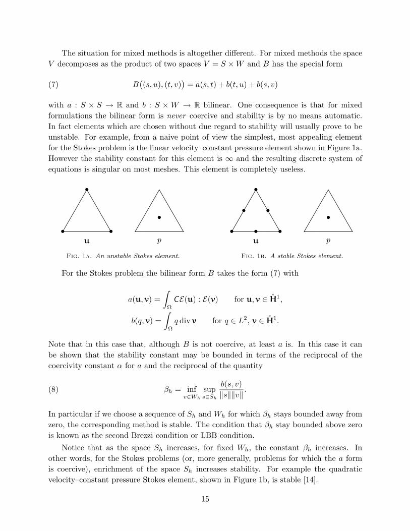
with a : S × S → R and b : S ×W → R bilinear. One consequence is that for mixedformulations the bilinear form is never coercive and stability is by no means automatic.In fact elements which are chosen without due regard to stability will usually prove to beunstable. For example, from a naive point of view the simplest, most appealing elementfor the Stokes problem is the linear velocity–constant pressure element shown in Figure 1a.However the stability constant for this element is ∞ and the resulting discrete system ofequations is singular on most meshes. This element is completely useless.

..................................................................................................................................................................................................................................................................................................................................................................................................................................................................... ................................................................................................................................................................

.....................................................................................................................................................................................................................................................................................................• •

•

•

u p

..................................................................................................................................................................................................................................................................................................................................................................................................................................................................... ................................................................................................................................................................

.....................................................................................................................................................................................................................................................................................................• •

•

•

• ••

u p

Fig. 1a. An unstable Stokes element. Fig. 1b. A stable Stokes element.

For the Stokes problem the bilinear form B takes the form (7) with

a(u, v) =∫

Ω

CE(u) : E(v) for u, v ∈ H1,

b(q, v) =∫

Ω

q div v for q ∈ L2, v ∈ H1.

Note that in this case that, although B is not coercive, at least a is. In this case it canbe shown that the stability constant may be bounded in terms of the reciprocal of thecoercivity constant α for a and the reciprocal of the quantity

(8) βh = infv∈Wh

sups∈Sh

b(s, v)‖s‖‖v‖

.

In particular if we choose a sequence of Sh and Wh for which βh stays bounded away fromzero, the corresponding method is stable. The condition that βh stay bounded above zerois known as the second Brezzi condition or LBB condition.

Notice that as the space Sh increases, for fixed Wh, the constant βh increases. Inother words, for the Stokes problems (or, more generally, problems for which the a formis coercive), enrichment of the space Sh increases stability. For example the quadraticvelocity–constant pressure Stokes element, shown in Figure 1b, is stable [14].

15

However the condition that the a form be coercive is not satisfied for most mixedmethods. In fact, of the four mixed formulations presented, only that for the Stokesproblem has this property. For the elasticity problem, for example, we have a(T , T ) =∫

ΩAT : T . Since it is possible to find T which is bounded by 1 everywhere but for

which the divergence of T is arbitrarily large, there cannot exist a constant α such thata(T , T ) ≥ ‖T‖2H(div) for all T in H(div). So the a form is indeed not coercive.

However, it turns out that one can get by with a weaker condition than coercivity ofa on S, namely coercivity on a particular subspace of Sh. More precisely, suppose thatthere exists a positive constant αh such that

(9) a(z, z) ≥ αh‖z‖2 for all z ∈ Zh

whereZh = z ∈ Sh | b(z, v) = 0 for all v ∈Wh.

Then the stability constant may be bounded in terms of the reciprocals of the constants αhin (9) and βh in (8). Thus if for a sequence of subspaces Sh ×Wh the αh remain boundeduniformly above zero (this is the first Brezzi condition), and the βh do likewise (secondBrezzi condition), then the resulting method is stable. This is the content of Brezzi’stheorem [10].

Let us briefly indicate the idea behind the theorem. Stability refers to the invertibilityof the matrix representing the discrete problem, and the stability constant is the norm ofthe inverse matrix. For mixed methods, the matrix has the form

(10)(A BtB 0

):ShWh

→ShWh

.

The space Zh introduced above is the nullspace of the B. Therefore, if we partition Sh asZh ×Z⊥h , where Z⊥h denotes the orthogonal complement of Zh in Sh, then the action of Bon Sh may be written as

( 0 B ) :ZhZ⊥h

→Wh

where B denotes the restriction of B to Z⊥h . Now the second Brezzi condition just assertsthe invertibility of B. Similarly, let us decompose the action of A as, say,(

A QR S

):ZhZ⊥h

→ZhZ⊥h

Thus A is the matrix associated with the bilinear form a restricted to Zh × Zh, and thefirst Brezzi condition simply asserts the invertibility of this operator. The whole matrix(10), rewritten in terms of these new notations, is A Q 0

R S Bt0 B 0

:

ZhZ⊥hWh

→

ZhZ⊥hWh

,

16

or, rearranging rows and columns, Bt R S0 A Q0 0 B

:

Wh

ZhZ⊥h

→

Z⊥hZhWh

.

From the upper triangular form, it is clear that the invertibility of B (which is equivalentto the invertibility of Bt) and the invertibility of A are together are necessary and sufficientfor the invertibility of the whole matrix.

While Brezzi’s theorem furnishes us with relatively concrete conditions which yieldstability, the verification of these conditions can be quite difficult. A number of analytictechniques have been developed that ease the task some what, for example, localizationtheorems [9], the use special mesh-dependent norms [7], etc. We shall not go into any ofthese techniques here, but in the next section we discuss a number of elements that have,in one way or another, been shown to be stable.

6. The construction of stable mixed elements. In § 4 we saw that the accuracyof a finite element discretization is determined by the approximability of the exact solutionby the finite element subspace and the stability of the discretization. These two properties,together with implementational issues, furnish the major factors for the construction andevaluation of the finite element spaces to be used. In § 5 we saw that stability is automaticfor coercive methods, such as most displacement methods, so that the finite element spacecan be chosen on the basis of approximation and ease of implementation alone. However,for mixed methods the question of stability is paramount.

Various techniques have been developed for the design of stable mixed elements. Inthis section we review some of these techniques and some of the resulting elements. Weemphasize that this review is by no means exhaustive, neither with regard to the techniquesnor to the resulting methods.

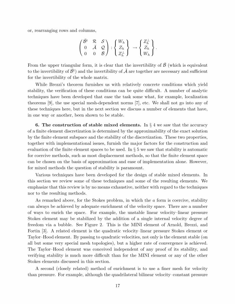
As remarked above, for the Stokes problem, in which the a form is coercive, stabilitycan always be achieved by adequate enrichment of the velocity space. There are a numberof ways to enrich the space. For example, the unstable linear velocity–linear pressureStokes element may be stabilized by the addition of a single internal velocity degree offreedom via a bubble. See Figure 2. This is the MINI element of Arnold, Brezzi, andFortin [3]. A related element is the quadratic velocity–linear pressure Stokes element orTaylor–Hood element. By passing to quadratic velocities, not only is the element stable (onall but some very special mesh topologies), but a higher rate of convergence is achieved.The Taylor–Hood element was conceived independent of any proof of its stability, andverifying stability is much more difficult than for the MINI element or any of the otherStokes elements discussed in this section.

A second (closely related) method of enrichment is to use a finer mesh for velocitythan pressure. For example, although the quadrilateral bilinear velocity–constant pressure

17

..................................................................................................................................................................................................................................................................................................................................................................................................................................................................... ................................................................................................................................................................

.....................................................................................................................................................................................................................................................................................................• •

•

• •

•

•u p

..................................................................................................................................................................................................................................................................................................................................................................................................................................................................... ................................................................................................................................................................

.....................................................................................................................................................................................................................................................................................................• •

•

•

•

• •

•

•u p

Fig. 2. An unstable Stokes element (left), stabilized by a bubble degree-of-freedom (right).

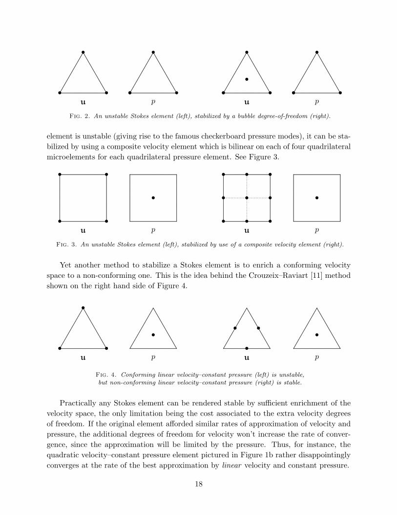
element is unstable (giving rise to the famous checkerboard pressure modes), it can be sta-bilized by using a composite velocity element which is bilinear on each of four quadrilateralmicroelements for each quadrilateral pressure element. See Figure 3.

..

..

..

..

..

..

..

..

..

..

..

..

..

..

..

.

...............................

............................................................................................................................................................................................................................................................................................................................................................................................................................................................................................................................................................................................................................ ...............................................................................................................................................................

........

........

........

........

........

........

........

........

........

........

........

........

........

........

........

........

........

.....................................................................................................................................................................................................................................................................................................................• •

••

•

u p

............................................................................................................................................................................................................................................................................................................................................................................................................................................................................................................................................................................................................................ ...............................................................................................................................................................

........

........

........

........

........

........

........

........

........

........

........

........

........

........

........

........

........

.....................................................................................................................................................................................................................................................................................................................• •

••

•

•

•

• • •

u p

Fig. 3. An unstable Stokes element (left), stabilized by use of a composite velocity element (right).

Yet another method to stabilize a Stokes element is to enrich a conforming velocityspace to a non-conforming one. This is the idea behind the Crouzeix–Raviart [11] methodshown on the right hand side of Figure 4.

..................................................................................................................................................................................................................................................................................................................................................................................................................................................................... ................................................................................................................................................................

.....................................................................................................................................................................................................................................................................................................• •

•

•

u p

..................................................................................................................................................................................................................................................................................................................................................................................................................................................................... ................................................................................................................................................................

.....................................................................................................................................................................................................................................................................................................•

• ••

u p

Fig. 4. Conforming linear velocity–constant pressure (left) is unstable,but non-conforming linear velocity–constant pressure (right) is stable.

Practically any Stokes element can be rendered stable by sufficient enrichment of thevelocity space, the only limitation being the cost associated to the extra velocity degreesof freedom. If the original element afforded similar rates of approximation of velocity andpressure, the additional degrees of freedom for velocity won’t increase the rate of conver-gence, since the approximation will be limited by the pressure. Thus, for instance, thequadratic velocity–constant pressure element pictured in Figure 1b rather disappointinglyconverges at the rate of the best approximation by linear velocity and constant pressure.

18

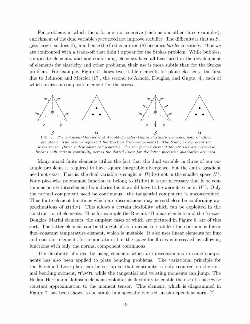
For problems in which the a form is not coercive (such as our other three examples),enrichment of the dual variable space need not improve stability. The difficulty is that as Shgets larger, so does Zh, and hence the first condition (8) becomes harder to satisfy. Thus weare confronted with a trade-off that didn’t appear for the Stokes problem. While bubbles,composite elements, and non-conforming elements have all been used in the developmentof elements for elasticity and other problems, their use is more subtle than for the Stokesproblem. For example, Figure 5 shows two stable elements for plane elasticity, the firstdue to Johnson and Mercier [17], the second to Arnold, Douglas, and Gupta [4], each ofwhich utilizes a composite element for the stress.

......

......

.......................

......

......

......

......

......

.......................

......

......

......

..................................................................................................................................................................................................................................................................................................................................................................................................................................................................... ................................................................................................................................................................

............................................................................................................................................................................................................................................................................................................................................

..........................

.................................................................

.................................................................

.................................................................

................................................

.................

...............................................

.................

................................................ • •

•

S u

..................................................................................................................................................................................................................................................................................................................................................................................................................................................................... ................................................................................................................................................................

............................................................................................................................................................................................................................................................................................................................................

..........................

.................................................................

.................................................................

.................................................................

................................................

.................

...............................................

.................

.................................................................

................................................................. ................

.................................................

................................................ • •

•

S uFig. 5. The Johnson–Mercier and Arnold–Douglas–Gupta elasticity elements, both of which

are stable. The arrows represent the traction (two components). The triangles represent thestress tensor (three independent components). For the former element the stresses are piecewise

linears with certain continuity across the dotted lines; for the latter piecewise quadratics are used.

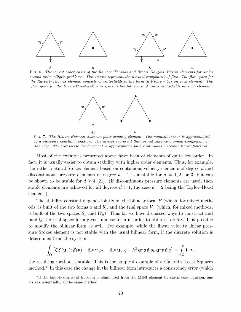
Many mixed finite elements utilize the fact that the dual variable in three of our ex-ample problems is required to have square integrable divergence, but the entire gradientneed not exist. That is, the dual variable is sought in H(div) not in the smaller space H1.For a piecewise polynomial function to belong to H(div) it is not necessary that it be con-tinuous across interelement boundaries (as it would have to be were it to lie in H1). Onlythe normal component need be continuous—the tangential component is unconstrained.Thus finite element functions which are discontinous may nevertheless be conforming ap-proximations of H(div). This allows a certain flexibility which can be exploited in theconstruction of elements. Thus for example the Raviart–Thomas elements and the Brezzi–Douglas–Marini elements, the simplest cases of which are pictured in Figure 6, are of thissort. The latter element can be thought of as a means to stabilize the continuous linearflux–constant temperature element, which is unstable. It also uses linear elements for fluxand constant elements for temperature, but the space for fluxes is increased by allowingfunctions with only the normal component continuous.

The flexibility afforded by using elements which are discontinuous in some compo-nents has also been applied to plate bending problems. The variational principle forthe Kirchhoff–Love plate can be set up so that continuity is only required on the nor-mal bending moment, ntMn, while the tangential and twisting moments can jump. TheHellan–Herrmann–Johnson element exploits this flexibility to enable the use of a piecewiseconstant approximation to the moment tensor. This element, which is diagrammed inFigure 7, has been shown to be stable in a specially devised, mesh-dependent norm [7].

19

..................................................................................................................................................................................................................................................................................................................................................................................................................................................................... ................................................................................................................................................................

............................................................................................................................................................................................................................................................................................................................................

..........................

................................................................. ................

.................................................

•

s u

..................................................................................................................................................................................................................................................................................................................................................................................................................................................................... ................................................................................................................................................................

............................................................................................................................................................................................................................................................................................................................................

..........................

.................................................................

.................................................................

.................................................................

................................................

.................

...............................................

.................

•

s uFig. 6. The lowest order cases of the Raviart–Thomas and Brezzi–Douglas–Marini elements for scalarsecond order elliptic problems. The arrows represent the normal component of flux. The flux space for

the Raviart–Thomas element consists of vectorfields of the form (a+ bx, c+ by) on each element. Theflux space for the Brezzi-Douglas-Marini space is the full space of linear vectorfields on each element.

..................................................................................................................................................................................................................................................................................................................................................................................................................................................................... ................................................................................................................................................................

............................................................................................................................................................................................................................................................................................................................................

..........................

................................................................. ................

.................................................

• •

•

•

M wFig. 7. The Hellan–Herman–Johnson plate bending element. The moment tensor is approximatedby a piecewise constant function. The arrows represent the normal bending moment component on

the edge. The transverse displacement is approximated by a continuous piecewise linear function.

Most of the examples presented above have been of elements of quite low order. Infact, it is usually easier to obtain stability with higher order elements. Thus, for example,the rather natural Stokes element based on continuous velocity elements of degree d anddiscontinuous pressure elements of degree d − 1 is unstable for d = 1, 2, or 3, but canbe shown to be stable for d ≥ 4 [21]. (If discontinuous pressure elements are used, thenstable elements are achieved for all degrees d > 1, the case d = 2 being the Taylor–Hoodelement.)

The stability constant depends jointly on the bilinear form B (which, for mixed meth-ods, is built of the two forms a and b), and the trial space Vh (which, for mixed methods,is built of the two spaces Sh and Wh). Thus far we have discussed ways to construct andmodify the trial space for a given bilinear form in order to obtain stability. It is possibleto modify the bilinear form as well. For example, while the linear velocity–linear pres-sure Stokes element is not stable with the usual bilinear form, if the discrete solution isdetermined from the system∫

Ω

[CE(uh) :E(v) + div v ph + divuh q − h2 grad ph grad q

]=∫

Ω

f · v,

the resulting method is stable. This is the simplest example of a Galerkin–Least Squaresmethod.* In this case the change in the bilinear form introduces a consistency error (which

*If the bubble degree of freedom is eliminated from the MINI element by static condensation, onearrives, essentially, at the same method.

20

however is small enough not to affect the rate of convergence). It is also possible to modifythe bilinear form in a consistent way and still have the linear/linear element stable [16]. Inthe last five years there have been numerous papers presenting extensions and variationsof this procedure to obtain simple, stable mixed methods for a variety of problems.

An alteration of the mixed variational formulation for elasticity of an entirely differentsort was introduced by Arnold and Falk [5]. They derived a variational principle involvingthe displacement field and a second-order tensorfield called the pseudostress, from whichthe true stress can easily be recovered as a linear combiniation of components. Theirnew variational principle is very similar to the Hellinger–Reissner principle but does notrequire a symmetry constraint on the tensorfield. This allows one to easily adapt mixedelements for the scalar second order elliptic problem, such as the Raviart–Thomas orBrezzi–Douglas–Marini elements described above.

REFERENCES

[1] D. N. Arnold, Discretization by finite elements of a model parameter dependent problem, Numer.

Math., 37 (1981), pp. 405–421.

[2] D. N. Arnold and F. Brezzi, Mixed and nonconforming finite element methods: implementation,

postprocessing and error estimates, Math. Modelling and Numer. Anal., 19 (1985), pp. 7–32.

[3] D. N. Arnold, F. Brezzi, and M. Fortin, A stable finite element for the Stokes equations,Calcolo, 21 (1984), pp. 337–344.

[4] D. N. Arnold, J. Douglas, and C. Gupta, A family of higher order mixed finite elementmethods for plane elasticity, Numer. Math., 45 (1984), pp. 1–22.

[5] D. N. Arnold and R. S. Falk, A new mixed formulation for elasticity, Numer. Math., 53 (1988),

pp. 13–30.

[6] I. Babuska and J. E. Osborn, Generalized finite element methods: their performance and their

relation to mixed methods, SIAM J. Numer. Anal., 20 (1983), pp. 510–536.

[7] I. Babuska, J. E. Osborn, and J. Pitkaranta, Analysis of mixed methods using mesh-dependentnorms, Math. Comp., 35 (1980), pp. 1039–1062.

[8] K. J. Bathe and F. Brezzi, On the convergence of a four-node plate bending element based on

Mindlin/Reissner plate theory and a mixed interpolation, in Mathematics of Finite Elements

and Applications V, J. R. Whiteman, ed., Academic Press, New York, NY, 1985, pp. 491–503.

[9] J. Boland and R. Nicolaides, Stability of finite elements under divergence constraints, SIAM J.Numer. Anal., 20 (1983), pp. 722–731.

[10] F. Brezzi, On the existence, uniqueness, and approximation of saddle point problems arising from

Lagrangian multipliers, RAIRO Anal. Numer., 8–32 (1974), pp. 129–151.

[11] M. Crouzeix and P. -A. Raviart, Conforming and non conforming finite element methods for

solving the stationary Stokes equations, RAIRO Anal. Numer., R3 (1973), pp. 33–76.

[12] B. Darlow, R. Ewing, and M. Wheeler, Mixed finite element methods for miscible displacement

in porous media, Sixth SPE Symposium on Reservoir Simulation, SPE 10501, New Orleans,1982.

[13] R. Ewing, T. Russell, and M. Wheeler, Simulation of miscible displacement using mixed

methods and a modified method of characteristics, Seventh SPE Symposium on Reservoir Sim-ulation, SPE 12241, San Francisco, 1983.

[14] M. Fortin, Calcul numerique des ecoulements des fluides de Bingham et des fluides Newtoniensincompressible par la methode es elements finis, Univ. Paris, Thesis, 1972.

21

[15] B. X. Fraeijs de Veubeke, Displacement and equilibrium models in the finite element method,in Stress Analysis, O. C. Zienkiewicz and G. Hollister, eds., John Wiley & Sons, New York,

NY, 1965.

[16] T. J. R. Hughes, L. P. Franca, and M. Balestra, A new finite element formulation for com-

putational fluid mechanics: V. Circumventing the Babuska–Brezzi condition: a stable Petrov–Galerkin formulation of the Stokes problem accounting for equal order interpolation, Comput.

Methods Appl. Mech. Engrg., 59 (1986), pp. 85–99.

[17] C. Johnson and B. Mercier, Some equilbrium finite element methods for two-dimensional elas-

ticity problems, Numer. Math., 30 (1978), pp. 103–116.

[18] C. Johnson and J. Pitkaranta, Analysis of some mixed finite element methods related to reducedintegration, Math. Comp., 38 (1982), pp. 375–400.

[19] D. S. Malkus and T. J. R. Hughes, Mixed finite element methods—reduced and selective inte-gration techniques: a unification of concepts, Comput. Methods Appl. Mech. Engrg., 15 (1978),

pp. 63–81.

[20] L. D. Marini and A. Savini, Accurate computation of electric field in reverse-biased semiconductor

devices: a mixed finite element approach, Compel, 3 (1984), pp. 123–135.

[21] L. R. Scott and M. Vogelius, Norm estimates for a maximal right inverse of the divergenceoperator in spaces of piecewise polynomials, RAIRO Model. Math. Anal. Numer., 19 (1985),

pp. 111–143.

22