Mining Spatio-temporal Data of Traffic Accidents and ... · Mining Spatio-temporal Data of Traffic Accidents and Spatial Pattern ... the analysis of spatial and time stamped data

Metodološki zvezki, Vol. 5, No. 1, 2008, 45-63

Mining Spatio-temporal Data of Traffic Accidents and Spatial Pattern Visualization

Nada Lavrač1,2, Domen Jesenovec1, Nejc Trdin1, and Neža Mramor Kosta3

Abstract

Spatial data mining is a research area concerned with the identification of interesting spatial patterns from data stored in spatial databases and geographic information systems (GIS). This paper addresses the analysis of spatial and time stamped data of Slovenian traffic accidents which, together with other GIS data, enabled the construction of spatial attributes and the creation of a time-stamped spatial database. This database was analyzed by means of basic descriptive statistical methods, an approach to short time series clustering, spatial clustering, as well as visualization using GIS and GoogleEarth facilities.

1 Introduction

Spatial data mining (Han et al., 2001; Han and Kamber, 2001) is a new and rapidly developing area of data mining (Han and Kamber, 2001; Tan et al., 2006), concerned with the identification of interesting spatial patterns from data stored in spatial databases and geographic information systems. Geographic information systems (Bernhardsen, 2002) enable capturing, storing, analyzing, and managing data and associated attributes which are spatially referenced to the Earth. GIS are used in various areas such as environmental impact assessment, urban planning, cartography, criminology, traffic analysis, etc. Collection of data is enabled by global positioning systems (GPS) and sensor networks, while computer storage technology enables the storage of enormous quantities of collected data. These advanced technologies are the reason for the existence of a growing number of spatial databases. The size of spatial databases, and the complexity of dealing with spatial attributes require the use of specialized data mining techniques (Han et al., 2001; Han and Kamber, 2001).

1 Jožef Stefan Institute, Jamova 39, 1000 Ljubljana, Slovenia 2 University of Nova Gorica, Vipavska 13, 5000 Nova Gorica, Slovenia 3 Faculty of computer and information sciences, Tržaška 25, 1000 Ljubljana, Slovenia

46 Nada Lavrač et al.

Data mining can significantly help improving traffic safety, and has been used in many traffic related studies (Chong et al., 2005; Flach et al., 2003; Tesema et al., 2005). In this study, a time-stamped database of Slovenian traffic accidents was analyzed by means of selected data visualization methods, an approach to short time series clustering, as well as clustering and spatial cluster visualization with GIS tools and the GoogleEarth facility.

A first step in understanding and mining the data for relevant information is a good choice of data visualization techniques, graphs and diagrams. In traffic data, traffic density patterns on hourly, weekly, and monthly scales can be obtained from density plots. Such plots identify traffic peaks, and can be of help to traffic specialists in planning routes and safety measures, as well as to individual drivers. Various trends, for example in the total number of accidents and in the number of accidents with serious injuries, presented on graphs, enable an overall analysis of traffic safety.

Temporal analysis of the traffic accidents is performed using methods of short time series analysis (Todorovski et al., 2003). A time series is a very common type of data, and there are many available algorithms and methods for time series analysis. In this work, time series clustering was used to identify groups of similar time series obtained for all Slovenian municipalities. We analyze two types of time series: the number of accidents by month and the number of accidents over the 11 years included in the database. Both types of time series considered are of the type referred to as short time series (consisting of 4-20 measurements), where a different approach to clustering is required than the approaches used for clustering of long time series. Short time series clustering has recently become popular due to its practical applications in biology (DNA microarray analysis) and economics. An approach to qualitative clustering of short time series of traffic accidents is one of the contributions of this paper.

The analysis of spatial aspects of the traffic accident database was performed by spatial clustering (Han et al., 2001; Han and Kamber, 2001) and cluster visualization in GIS and GoogleEarth. GoogleEarth4 is a program, freely available for users on the internet, whose main functionality is viewing satellite images of the whole Earth surface. Additionally it can display external layers of data on satellite images. GoogleEarth visualization of traffic accidents cluster centroids is another methodological contribution of this paper.

The structure of this paper is as follows. Section 2 describes data preparation and the constructed spatial database. Section 3 presents the results of the selected data visualization tools, and compares the results of Slovenian traffic accidents analysis with those of traffic accident analysis in the UK (Flach et al., 2003). In Section 4 short time series clustering is presented. Section 5 presents the program for identifying clusters of accidents, and the visualization of discovered clusters

4 GoogleEarth web page: http://earth.google.com

Mining Spatio-temporal Data of Traffic Accidents… 47

using GoogleEarth. We conclude with a discussion and some ideas for future work in Section 6.

2 Traffic accident data

In this research two traffic accident datasets were used: (a) the database of Slovenian traffic accidents, including data on accidents in Slovenia between the years 1995 and 2005, which is in text file format and is publicly available on the internet5, and (b) the database obtained directly from the Slovenian police, which includes also the data for year 2006. The publicly available data has no geographic attributes; this data was used for short time series clustering described in Section 3. On the other hand, the police database of traffic accidents includes also geographic locations of accidents; this data was used for spatial clustering described in Section 4.

2.1 Data format and data preprocessing

In order to transform the text files available on the internet into a format, appropriate for database storage, a substantial amount of data preprocessing was needed. The format of the text files and the values of certain attributes which changed over the years were unified, missing values were handled and some attributes were discretized. Most importantly, geographic data (GIS data of precise locations of accidents), additionally acquired from a database obtained from the Slovenian police was added.

In geographic information systems there are two ways of storing and representing spatial data (Bernhardsen, 2002): the vector and raster representation. Vector representation consists of descriptions of spatial objects (points, lines, polygons). In raster representation, the Earth surface is divided into a grid of square cells, and these cells are described. Vector data is storage efficient and accurate, but requires complex computations. Raster data is just the opposite: less accurate and simpler to handle. In the GIS database acquired from the Slovenian police, the geographic data is contained in the vector based shape files (SHP) 6. Using the R programming language7 and the shape files package, spatial attributes were extracted from the SHP files and added to the existing relational database. In this process, a transformation of the coordinate system was also performed using

5 Slovenian traffic accident data: http://www.policija.si/portal/statistika/promet/promet.php 6 The SHP file format, developed and regulated by the US software company ESRI, is a de

facto standard for storing vector spatial data. The shapefiles package commonly refers to a collection of files with shp, shx and dbf extensions (SHP contains definitions of spatial objects, DBF the data associated with objects, and SHX stores the index of the feature geometry).

7 R web page: http://cran.r-project.org


the PROJ.4 program8 from the D48 coordinate system (Slovenian national coordinate system) to the generally used system WGS84.

2.2 Database of Slovenian traffic accidents

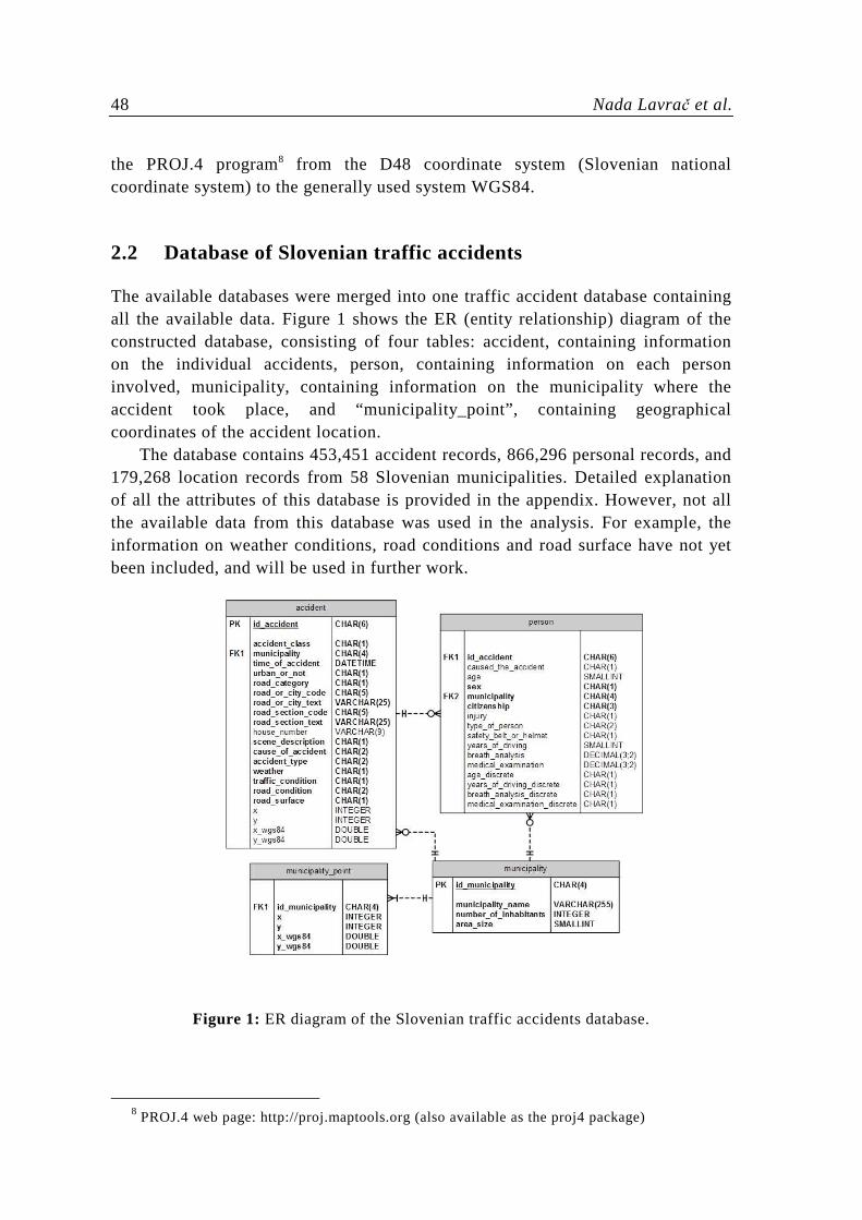
The available databases were merged into one traffic accident database containing all the available data. Figure 1 shows the ER (entity relationship) diagram of the constructed database, consisting of four tables: accident, containing information on the individual accidents, person, containing information on each person involved, municipality, containing information on the municipality where the accident took place, and “municipality_point”, containing geographical coordinates of the accident location.

The database contains 453,451 accident records, 866,296 personal records, and 179,268 location records from 58 Slovenian municipalities. Detailed explanation of all the attributes of this database is provided in the appendix. However, not all the available data from this database was used in the analysis. For example, the information on weather conditions, road conditions and road surface have not yet been included, and will be used in further work.

Figure 1: ER diagram of the Slovenian traffic accidents database.

8 PROJ.4 web page: http://proj.maptools.org (also available as the proj4 package)


2.3 Data visualization

The first step in the data mining process was data visualization, performed to enable better understanding of the data. Selected visualizations are presented below.

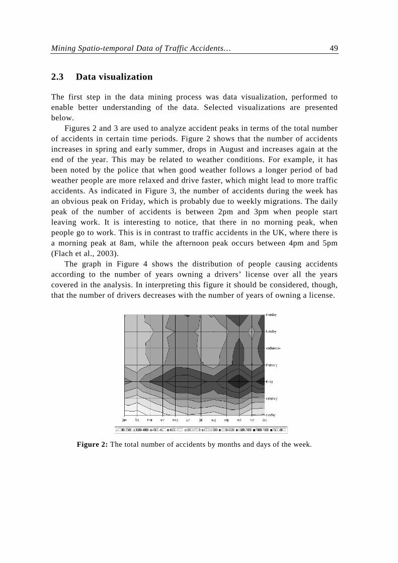
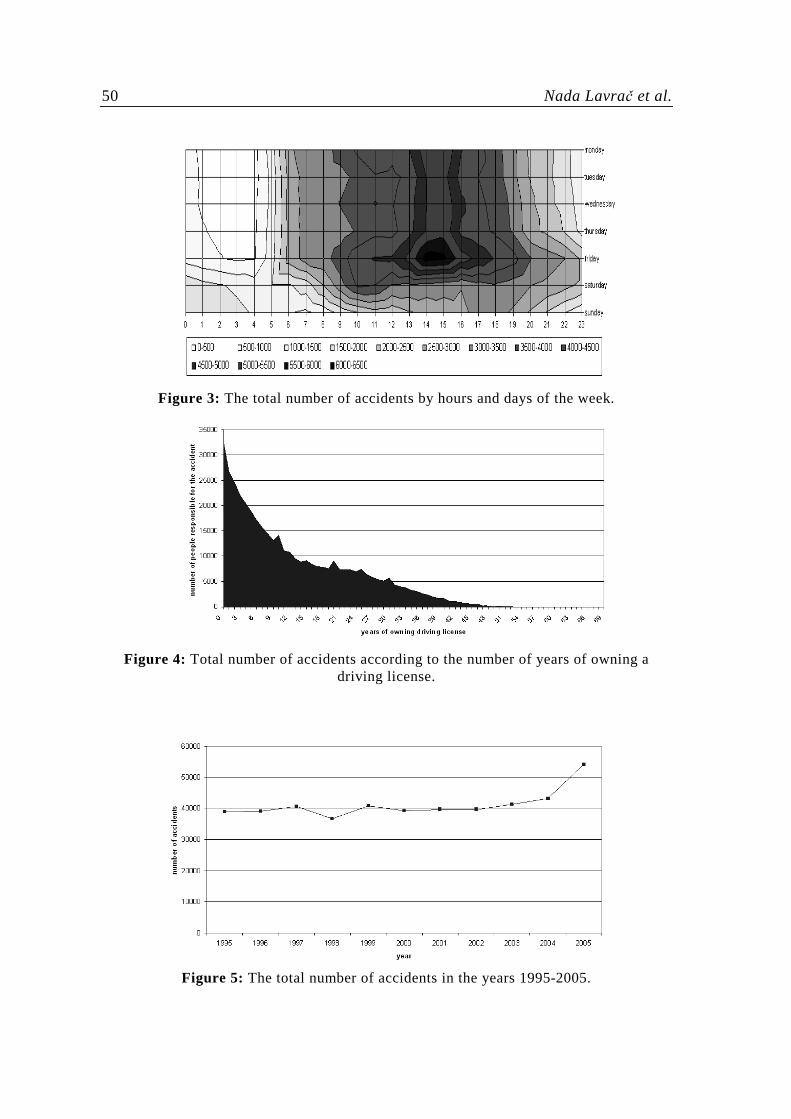
Figures 2 and 3 are used to analyze accident peaks in terms of the total number of accidents in certain time periods. Figure 2 shows that the number of accidents increases in spring and early summer, drops in August and increases again at the end of the year. This may be related to weather conditions. For example, it has been noted by the police that when good weather follows a longer period of bad weather people are more relaxed and drive faster, which might lead to more traffic accidents. As indicated in Figure 3, the number of accidents during the week has an obvious peak on Friday, which is probably due to weekly migrations. The daily peak of the number of accidents is between 2pm and 3pm when people start leaving work. It is interesting to notice, that there in no morning peak, when people go to work. This is in contrast to traffic accidents in the UK, where there is a morning peak at 8am, while the afternoon peak occurs between 4pm and 5pm (Flach et al., 2003).

The graph in Figure 4 shows the distribution of people causing accidents according to the number of years owning a drivers’ license over all the years covered in the analysis. In interpreting this figure it should be considered, though, that the number of drivers decreases with the number of years of owning a license.

Figure 2: The total number of accidents by months and days of the week.


Figure 3: The total number of accidents by hours and days of the week.

Figure 4: Total number of accidents according to the number of years of owning a

driving license.

Figure 5: The total number of accidents in the years 1995-2005.


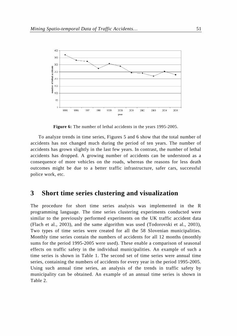
Figure 6: The number of lethal accidents in the years 1995-2005.

To analyze trends in time series, Figures 5 and 6 show that the total number of accidents has not changed much during the period of ten years. The number of accidents has grown slightly in the last few years. In contrast, the number of lethal accidents has dropped. A growing number of accidents can be understood as a consequence of more vehicles on the roads, whereas the reasons for less death outcomes might be due to a better traffic infrastructure, safer cars, successful police work, etc.

3 Short time series clustering and visualization

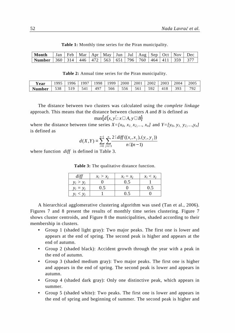
The procedure for short time series analysis was implemented in the R programming language. The time series clustering experiments conducted were similar to the previously performed experiments on the UK traffic accident data (Flach et al., 2003), and the same algorithm was used (Todorovski et al., 2003), Two types of time series were created for all the 58 Slovenian municipalities. Monthly time series contain the numbers of accidents for all 12 months (monthly sums for the period 1995-2005 were used). These enable a comparison of seasonal effects on traffic safety in the individual municipalities. An example of such a time series is shown in Table 1. The second set of time series were annual time series, containing the numbers of accidents for every year in the period 1995-2005. Using such annual time series, an analysis of the trends in traffic safety by municipality can be obtained. An example of an annual time series is shown in Table 2.


Table 1: Monthly time series for the Piran municipality.

Month Jan Feb Mar Apr May Jun Jul Aug Sep Oct Nov Dec Number 360 314 446 472 563 651 796 760 464 411 359 377

Table 2: Annual time series for the Piran municipality.

Year 1995 1996 1997 1998 1999 2000 2001 2002 2003 2004 2005

Number 538 519 541 497 566 556 561 592 418 393 792

The distance between two clusters was calculated using the complete linkage

approach. This means that the distance between clusters A and B is defined as ( ){ }ByAxyxd ∈∈ ,:,max

where the distance between time series X=[x 0, x1, x2,…, xn] and Y=[y0, y1, y2,…,yn] is defined as

∑∑−

= += −⋅⋅

=1

0 1 )1(

)),(),,((2),(

n

i

n

ij

jiji

nn

yyxxdiffYXd

where function diff is defined in Table 3.

Table 3: The qualitative distance function.

diff xi > xj xi = xj xi < xj yi > yj 0 0.5 1 yi = yj 0.5 0 0.5 yi < yj 1 0.5 0

A hierarchical agglomerative clustering algorithm was used (Tan et al., 2006).

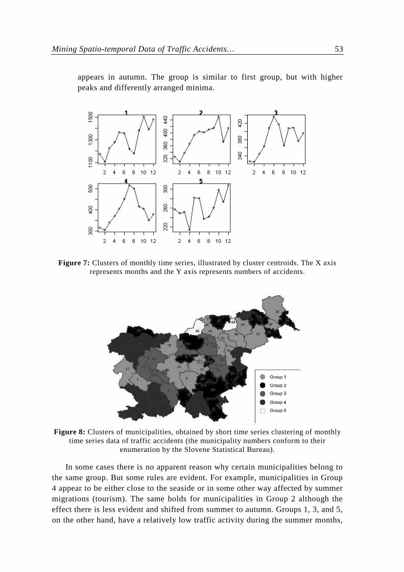
Figures 7 and 8 present the results of monthly time series clustering. Figure 7 shows cluster centroids, and Figure 8 the municipalities, shaded according to their membership in clusters.

• Group 1 (shaded light gray): Two major peaks. The first one is lower and appears at the end of spring. The second peak is higher and appears at the end of autumn.

• Group 2 (shaded black): Accident growth through the year with a peak in the end of autumn.

• Group 3 (shaded medium gray): Two major peaks. The first one is higher and appears in the end of spring. The second peak is lower and appears in autumn.

• Group 4 (shaded dark gray): Only one distinctive peak, which appears in summer.

• Group 5 (shaded white): Two peaks. The first one is lower and appears in the end of spring and beginning of summer. The second peak is higher and


appears in autumn. The group is similar to first group, but with higher peaks and differently arranged minima.

Figure 7: Clusters of monthly time series, illustrated by cluster centroids. The X axis

represents months and the Y axis represents numbers of accidents.

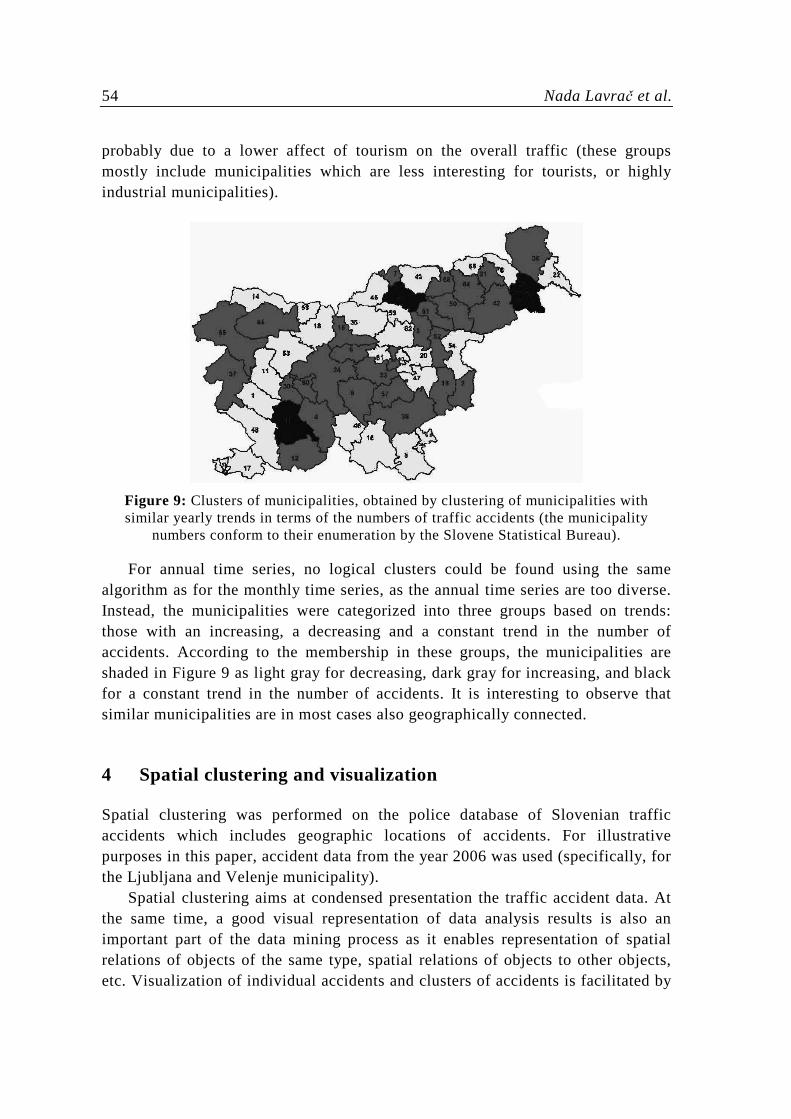
Figure 8: Clusters of municipalities, obtained by short time series clustering of monthly

time series data of traffic accidents (the municipality numbers conform to their enumeration by the Slovene Statistical Bureau).

In some cases there is no apparent reason why certain municipalities belong to the same group. But some rules are evident. For example, municipalities in Group 4 appear to be either close to the seaside or in some other way affected by summer migrations (tourism). The same holds for municipalities in Group 2 although the effect there is less evident and shifted from summer to autumn. Groups 1, 3, and 5, on the other hand, have a relatively low traffic activity during the summer months,


probably due to a lower affect of tourism on the overall traffic (these groups mostly include municipalities which are less interesting for tourists, or highly industrial municipalities).

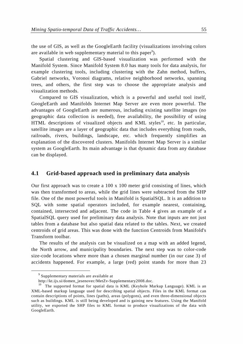
Figure 9: Clusters of municipalities, obtained by clustering of municipalities with similar yearly trends in terms of the numbers of traffic accidents (the municipality

numbers conform to their enumeration by the Slovene Statistical Bureau).

For annual time series, no logical clusters could be found using the same algorithm as for the monthly time series, as the annual time series are too diverse. Instead, the municipalities were categorized into three groups based on trends: those with an increasing, a decreasing and a constant trend in the number of accidents. According to the membership in these groups, the municipalities are shaded in Figure 9 as light gray for decreasing, dark gray for increasing, and black for a constant trend in the number of accidents. It is interesting to observe that similar municipalities are in most cases also geographically connected.

4 Spatial clustering and visualization

Spatial clustering was performed on the police database of Slovenian traffic accidents which includes geographic locations of accidents. For illustrative purposes in this paper, accident data from the year 2006 was used (specifically, for the Ljubljana and Velenje municipality).

Spatial clustering aims at condensed presentation the traffic accident data. At the same time, a good visual representation of data analysis results is also an important part of the data mining process as it enables representation of spatial relations of objects of the same type, spatial relations of objects to other objects, etc. Visualization of individual accidents and clusters of accidents is facilitated by


the use of GIS, as well as the GoogleEarth facility (visualizations involving colors are available in web supplementary material to this paper9).

Spatial clustering and GIS-based visualization was performed with the Manifold System. Since Manifold System 8.0 has many tools for data analysis, for example clustering tools, including clustering with the Zahn method, buffers, Gabriel networks, Voronoi diagrams, relative neighborhood networks, spanning trees, and others, the first step was to choose the appropriate analysis and visualization methods.

Compared to GIS visualization, which is a powerful and useful tool itself, GoogleEarth and Manifolds Internet Map Server are even more powerful. The advantages of GoogleEarth are numerous, including existing satellite images (no geographic data collection is needed), free availability, the possibility of using HTML descriptions of visualized objects and KML styles10, etc. In particular, satellite images are a layer of geographic data that includes everything from roads, railroads, rivers, buildings, landscape, etc. which frequently simplifies an explanation of the discovered clusters. Manifolds Internet Map Server is a similar system as GoogleEarth. Its main advantage is that dynamic data from any database can be displayed.

4.1 Grid-based approach used in preliminary data analysis

Our first approach was to create a 100 x 100 meter grid consisting of lines, which was then transformed to areas, while the grid lines were subtracted from the SHP file. One of the most powerful tools in Manifold is SpatialSQL. It is an addition to SQL with some spatial operators included, for example nearest, containing, contained, intersected and adjacent. The code in Table 4 gives an example of a SpatialSQL query used for preliminary data analysis. Note that inputs are not just tables from a database but also spatial data related to the tables. Next, we created centroids of grid areas. This was done with the function Centroids from Manifold's Transform toolbar.

The results of the analysis can be visualized on a map with an added legend, the North arrow, and municipality boundaries. The next step was to color-code size-code locations where more than a chosen marginal number (in our case 3) of accidents happened. For example, a large (red) point stands for more than 23

9 Supplementary materials are available at http://kt.ijs.si/domen_jesenovec/MetZv-Supplementary2008.doc. 10 The supported format for spatial data is KML (Keyhole Markup Language). KML is an

XML-based markup language used for describing spatial objects. Files in the KML format can contain descriptions of points, lines (paths), areas (polygons), and even three-dimensional objects such as buildings. KML is still being developed and is gaining new features. Using the Manifold utility, we exported the SHP files to KML format to produce visualizations of the data with GoogleEarth.


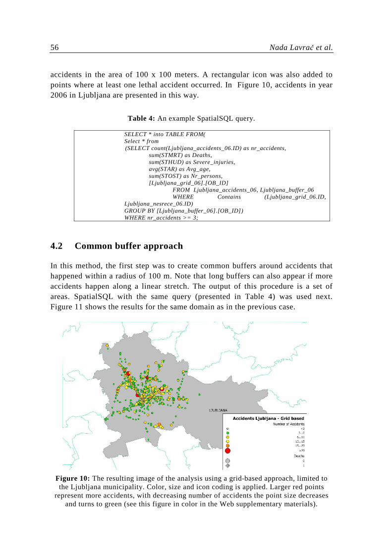
accidents in the area of 100 x 100 meters. A rectangular icon was also added to points where at least one lethal accident occurred. In Figure 10, accidents in year 2006 in Ljubljana are presented in this way.

Table 4: An example SpatialSQL query.

SELECT * into TABLE FROM( Select * from (SELECT count(Ljubljana_accidents_06.ID) as nr_accidents, sum(STMRT) as Deaths, sum(STHUD) as Severe_injuries, avg(STAR) as Avg_age, sum(STOST) as Nr_persons, [Ljubljana_grid_06].[OB_ID] FROM Ljubljana_accidents_06, Ljubljana_buffer_06 WHERE Contains (Ljubljana_grid_06.ID, Ljubljana_nesrece_06.ID) GROUP BY [Ljubljana_buffer_06].[OB_ID]) WHERE nr_accidents >= 3;

4.2 Common buffer approach

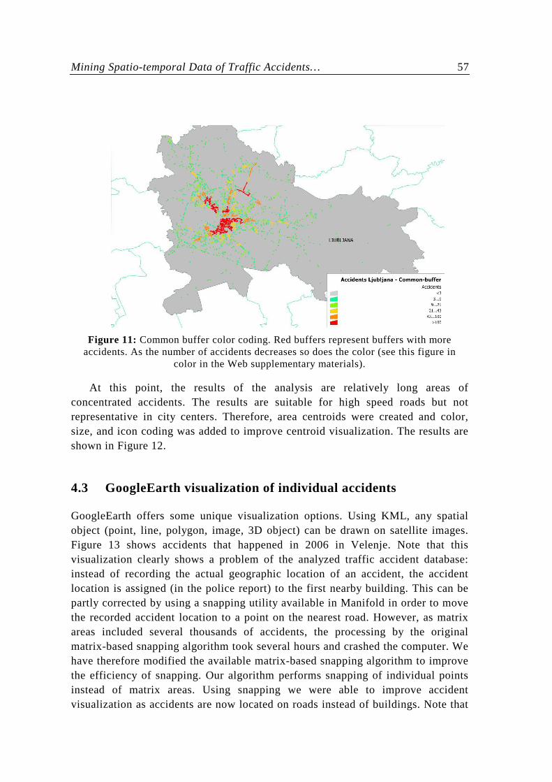
In this method, the first step was to create common buffers around accidents that happened within a radius of 100 m. Note that long buffers can also appear if more accidents happen along a linear stretch. The output of this procedure is a set of areas. SpatialSQL with the same query (presented in Table 4) was used next. Figure 11 shows the results for the same domain as in the previous case.

Figure 10: The resulting image of the analysis using a grid-based approach, limited to the Ljubljana municipality. Color, size and icon coding is applied. Larger red points

represent more accidents, with decreasing number of accidents the point size decreases and turns to green (see this figure in color in the Web supplementary materials).


Figure 11: Common buffer color coding. Red buffers represent buffers with more

accidents. As the number of accidents decreases so does the color (see this figure in color in the Web supplementary materials).

At this point, the results of the analysis are relatively long areas of concentrated accidents. The results are suitable for high speed roads but not representative in city centers. Therefore, area centroids were created and color, size, and icon coding was added to improve centroid visualization. The results are shown in Figure 12.

4.3 GoogleEarth visualization of individual accidents

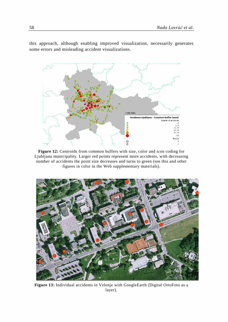
GoogleEarth offers some unique visualization options. Using KML, any spatial object (point, line, polygon, image, 3D object) can be drawn on satellite images. Figure 13 shows accidents that happened in 2006 in Velenje. Note that this visualization clearly shows a problem of the analyzed traffic accident database: instead of recording the actual geographic location of an accident, the accident location is assigned (in the police report) to the first nearby building. This can be partly corrected by using a snapping utility available in Manifold in order to move the recorded accident location to a point on the nearest road. However, as matrix areas included several thousands of accidents, the processing by the original matrix-based snapping algorithm took several hours and crashed the computer. We have therefore modified the available matrix-based snapping algorithm to improve the efficiency of snapping. Our algorithm performs snapping of individual points instead of matrix areas. Using snapping we were able to improve accident visualization as accidents are now located on roads instead of buildings. Note that


this approach, although enabling improved visualization, necessarily generates some errors and misleading accident visualizations.

Figure 12: Centroids from common buffers with size, color and icon coding for

Ljubljana municipality. Larger red points represent more accidents, with decreasing number of accidents the point size decreases and turns to green (see this and other

figures in color in the Web supplementary materials).

Figure 13: Individual accidents in Velenje with GoogleEarth (Digital OrtoFoto as a

layer).


4.4 Zahn clustering and GoogleEarth cluster visualization

Accident clusters were generated by the Zahn clustering method implemented as a facility in the Manifold environment.

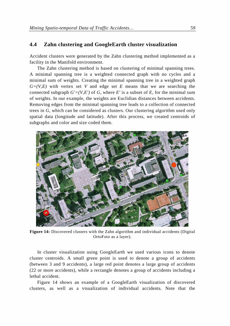
The Zahn clustering method is based on clustering of minimal spanning trees. A minimal spanning tree is a weighted connected graph with no cycles and a minimal sum of weights. Creating the minimal spanning tree in a weighted graph G=(V,E) with vertex set V and edge set E means that we are searching the connected subgraph G'=(V,E') of G, where E' is a subset of E, for the minimal sum of weights. In our example, the weights are Euclidian distances between accidents. Removing edges from the minimal spanning tree leads to a collection of connected trees in G, which can be considered as clusters. Our clustering algorithm used only spatial data (longitude and latitude). After this process, we created centroids of subgraphs and color and size coded them.

Figure 14: Discovered clusters with the Zahn algorithm and individual accidents (Digital

OrtoFoto as a layer).

In cluster visualization using GoogleEarth we used various icons to denote

cluster centroids. A small green point is used to denote a group of accidents (between 3 and 9 accidents), a large red point denotes a large group of accidents (22 or more accidents), while a rectangle denotes a group of accidents including a lethal accident.

Figure 14 shows an example of a GoogleEarth visualization of discovered clusters, as well as a visualization of individual accidents. Note that the


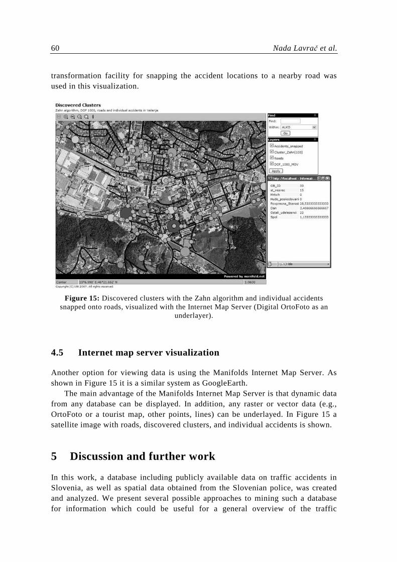
transformation facility for snapping the accident locations to a nearby road was used in this visualization.

Figure 15: Discovered clusters with the Zahn algorithm and individual accidents snapped onto roads, visualized with the Internet Map Server (Digital OrtoFoto as an

underlayer).

4.5 Internet map server visualization

Another option for viewing data is using the Manifolds Internet Map Server. As shown in Figure 15 it is a similar system as GoogleEarth.

The main advantage of the Manifolds Internet Map Server is that dynamic data from any database can be displayed. In addition, any raster or vector data (e.g., OrtoFoto or a tourist map, other points, lines) can be underlayed. In Figure 15 a satellite image with roads, discovered clusters, and individual accidents is shown.

5 Discussion and further work

In this work, a database including publicly available data on traffic accidents in Slovenia, as well as spatial data obtained from the Slovenian police, was created and analyzed. We present several possible approaches to mining such a database for information which could be useful for a general overview of the traffic


situation and trends and, in particular, to traffic experts in traffic planning and in improving traffic safety. Selected visualization methods which enable an insight into traffic accidents in all of Slovenia are demonstrated. Using short time series analysis and advanced visualization techniques, traffic safety in different municipalities (regions) and at different time periods has been analyzed and compared to the results of a similar research performed on UK traffic accident data. Nevertheless, the main focus of this work was on the use of spatial data mining techniques, of which association rules mining and clustering were used. The results of spatial association rule mining (using the SPADA algorithm; Appice et al., 2003) which have also been performed did not lead to results of sufficient interest, therefore the description of these experiments is not included in this paper. On the other hand, clustering is a well-understood and a very easily interpretable technique, which was well appreciated by traffic analysts. For presenting the results of accidents clustering the Manifold and the GoogleEarth programs were used, since they enable very powerful visualizations.

The database created contains information which has not been exploited yet, for example weather conditions and road condition at the accident location. These will be included in further work. Also, further time series analyses, for example a comparison of the monthly time series through the years, as well as additional clustering experiments, for example clustering of the day of week profiles by municipalities, might provide additional useful information. In cooperation with traffic experts we also hope to find explanations for some interesting features of the data discovered, and possible ways to use the results of this work in improving traffic safety in Slovenia.

Acknowledgements

We acknowledge the financial support of the Slovenian Ministry of Higher Education, Science and Technology programme Knowledge Technologies. We are also grateful to Ljupčo Todorovski, Sašo Džeroski and Peter Ljubič for previous joint work on short time series data analysis, Annalisa Appice for her support and expertise in the experiments with spatial association rule mining.

References

[1] Appice, A., Ceci, M., Lanza, A., Lisi, F.A., and Malerba, D. (2003): Discovery of spatial association rules in georeferenced census data: A relational mining approach. Intelligent Data Analysis, 7, 41-566.

[2] Bernhardsen, T. (2002): Geographic Information Systems: An Introduction, New York: Wiley.


[3] Chong, M., Abraham, A., and Paprzycki, M. (2005): Traffic accident data analysis using machine learning paradigms, Informatica: An International Journal of Computing and Informatics, 29, 89-98.

[4] Flach, P. et al. (2003): On the road to knowledge: Mining 21 years of UK traffic accident reports. In Mladenič, D., Lavrač, N., Bohanec, M., and Moyle, S. (Eds.): Data Mining and Decision Support: Integration and Collaboration, Kluwer Academic Publishers.

[5] Han, J., Kamber, M., and Tung, A. K. H. (2001): Spatial clustering methods in data mining: A survey. In Miller, H.J. and Han, J. (Eds.): Geographic Data Mining and Knowledge Discovery, 3-32, Taylor and Francis.

[6] Han, J. and Kamber, M. (2001): Data Mining: Concepts and Techniques, Morgan Kaufmann.

[7] Tan, P.-N., Steinbach, M., and Kumar, V. (2006): Introduction to Data Mining. Pearson Addison Wesley.

[8] Tesema, T.B., Abraham, A., and Grosan, C. (2005): Rule mining and classification of road traffic accidents using adaptive regression trees. International Journal of Simulation: Systems, Science & Technology, 6, 80-94.

[9] Todorovski, L., Ljubič, P., Lavrač, N., Džeroski, S., and Bellazzi, R. (2003): Qualitative clustering of short time series, Jožef Stefan Institute Technical Report, Ljubljana, Slovenia.

[10] Manifold System – The Ultimate GIS and Mapping package. Available at: http://www.manifold.net/index.shtml, 2008.

[11] Keyhole Markup Language - Wikipedia, the free encyclopedia. Available at: http://en.wikipedia.org/wiki/Keyhole_Markup_Language, 2007.

Appendix: Detailed description of attributes of the traffic accident database

(a) Attributes describing an accident: • id_accident – unique accident identifier, used in the police databases • accident_class – classifies the accident, depending on injuries (6 possible

values) • municipality – municipality where the accident occurred (58 possible

municipalities) • time_of_accident – date and time of the accident • urban_or_not – indicates whether the accident occurred inside an urban area

(y/n) • road_category – category of the road where the accident occurred (14

possible values) • road_or_city_code – code of the road or city where the accident occurred


• road_or_city_text – textual description of the road or city where the accident occurred

• house_number – house number (not always defined) • scene_description – describes the place of the accident (9 possible values) • cause_of_accident – what caused the accident (11 possible values) • accident_type – defines the type of accident (10 possible values) • weather – describes weather conditions at the time of the accident (8

possible values) • traffic_condition - describes traffic conditions (5 possible values) • road_condition – the condition of the road (9 possible values) • road_surface – e.g., asphalt, dirt (3 possible values) • x,y – coordinates of the accident acquired from SHP files (D48 coordinate

system) • x_wgs, y_wgs – coordinates of the accident in the international WGS84

system (b) Attributes describing each person involved in an accident:

• id_accident – this attribute connects the person to an individual accident • caused_the_accident – defines if the person caused the accident (y/n) • age – age of the person at the time of accident • sex – sex of the person (m/f) • municipality – municipality where the person lives • citizenship – citizenship of the person • injury – what injuries did the person acquire (6 possible values) • type_of_the_person – how was the person involved in the accident, e.g.,

pedestrian (23 possible values) • safety_belt_or_helmet – did the person use a safety belt or a helmet

(depending on the type of person) (y/n) • years_of_driving – how many years of driving experience does the person

have • breath_analysis – result of breath analysis, if performed • medical_examination – result of a medical examination (e.g., blood test), if

performed Four attributes were discretized for use in certain applications (age_discrete, years_of_driving_discrete, breath_analysis_discrete, medical_examination_discrete).

(c) Attributes describing the municipality of the accident: • id_municipality – unique municipality identifier • municipality_name – name of the municipality • number_of_inhabitants, area_size – attributes used to compare the

municipalities (d) Attributes describing municipality points: a table of points that define the borders of individual municipalities (this data is used for drawing the borders of municipalities; points are available in the D48 and WGS84 coordinate systems).

Documents

Mining Spatio-temporal Data of Traffic Accidents and ... · Mining Spatio-temporal Data of Traffic Accidents and Spatial Pattern ... the analysis of spatial and time stamped data