1

Microsimulations for Poverty and Inequality in Mexico using parameters from a

CGE Model

By

Araceli Ortega Díaz1

In the current paper we use microsimulations to analyze poverty and inequality through the accumulative impact on wages due to sequential changes in the labor market unemployment rate (U), employment structure (S), wages by economic sector (W1), average labor income (W2), and employment structure by skill level (M). These effects are based on the parameters obtained from a Computable General Equilibrium Model, with parameters allowing for simulations from 2003 to 2015. The microsimulations are applied to a national household’s survey, which distinguishes rural from urban households, and national from international poverty measures. The results show that an increment in the real wages will reduce extreme poverty by half. The changes in the employment structure and wages by economic sector reduce poverty due to workers moving from the agricultural sector to the service sector, implicitly allowing workers to move from sectors with lower wages to higher wages sectors. To reduce the number of people living under the food basket poverty line it is necessary to maintain sustainable increases in wages as this type of poverty is not substantially affected by changes in employment structure. It is found that changes in the employment structure by skill level is related to an increase in wage inequality as more skilled workers obtain better wages than unskilled employees. JEL Classification: C15, D6, D31, I32

1 Araceli Ortega is Professor at EGAP-ITESM, Monterrey Campus. The author would like to thank for the comments of the participants of the II General Conference of the International Microsimulation Association organized by Statistics Canada in June 2009.

2

Microsimulations for Poverty and Inequality in Mexico using parameters from a

CGE Model

By

Araceli Ortega Díaz2

Introduction

In January 2005, 19 Latin American Countries led by a UNDP-ECLAC-WB3 team started a project to assess the achievement of the Millennium Development Goals (MDGs) in each country. The project uses a Computable General Equilibrium Model (CGEM) which was complemented with microsimulations to assess the impact of achieving the MDG goals on income distribution and poverty. One important reason for performing a microsimulation analysis of poverty and inequality is that the CGEM uses aggregate micro data to model the impacts of macroeconomic policy decisions like fiscal or monetary policy, but due to its high level of aggregation of household structure it is difficult to obtain measures of income distribution and poverty, and it is necessary to implement microsimulation procedures using the CGEM parameters. In the current analysis we apply a simple microsimulation methodology to model the performance of poverty and inequality from 2003 to 2015, using the behavior of the labor market modeled through the parameters obtained from the CGEM. The CGEM parameters include workers skill levels, economic sector, wage and the unemployment rate of the economic sector. These parameters are applied to workers taken from the Income and Expenditure Household Survey (ENIGH-2002)4 according to their skill level and economic sector Every simulation in the CGEM gives us a new distribution of income due to the change in several parameters in the labor market. These parameters are introduced into the microsimulations to calculate the new income distribution and poverty. It is important to keep in mind that the microsimulation assumes that the only source of change in income distribution and poverty is changes in the labor market. The present analysis uses the parameters of the BAU (Business As Usual) scenario.

Mexico

2 The author is currently a lecturer at EGAP-ITESM campus Monterrey. She was Chief Advisor at the Subsecretary of Prospective, Planning and Evaluation within the Subsecretary of Social Development when she elaborated this analysis. The author thanks Elizabeth Monroy Cruz for her valuable assistance in this project. 3 UNDP stands for United Nations Development Program, ECLAC for Economic Commission for Latin America and the Caribbean, and WB stands for World Bank. 4 Workers in the official age range, which is 12 to 65 years old.

3

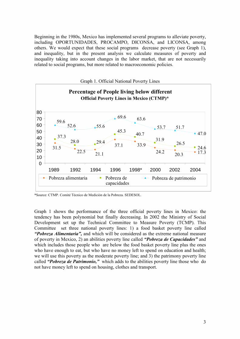
Beginning in the 1980s, Mexico has implemented several programs to alleviate poverty, including OPORTUNIDADES, PROCAMPO, DICONSA, and LICONSA, among others. We would expect that these social programs decrease poverty (see Graph 1), and inequality, but in the present analysis we calculate measures of poverty and inequality taking into account changes in the labor market, that are not necessarily related to social programs, but more related to macroeconomic policies.

Graph 1. Official National Poverty Lines

*Source: CTMP. Comité Técnico de Medición de la Pobreza. SEDESOL.

Graph 1 shows the performance of the three official poverty lines in Mexico: the tendency has been polynomial but finally decreasing. In 2002 the Ministry of Social Development set up the Technical Committee to Measure Poverty (TCMP). This Committee set three national poverty lines: 1) a food basket poverty line called “Pobreza Alimentaria”, and which will be considered as the extreme national measure of poverty in Mexico, 2) an abilities poverty line called “Pobreza de Capacidades” and which includes those people who are below the food basket poverty line plus the ones who have enough to eat, but who have no money left to spend on education and health; we will use this poverty as the moderate poverty line; and 3) the patrimony poverty line called “Pobreza de Patrimonio,” which adds to the abilities poverty line those who do not have money left to spend on housing, clothes and transport.

Percentage of People living below differentOfficial Poverty Lines in Mexico (CTMP)*

17.324.6

47.0

31.5 22.5

21.1

37.1 33.9

24.220.3

37.328.0 29.4 26.5

31.9 40.7

45.3

59.652.6 55.6

69.6 63.6

53.7 51.7

01020304050607080

1989 1992 1994 1996 1998* 2000 2002 2004

Pobreza alimentaria Pobreza de capacidades

Pobreza de patrimonio

4

We expect the microsimulations to shed some light on how these poverty lines will perform when there are changes in the labor market that result from changes in macroeconomic policies to achieve the Millennium development goals.

Data

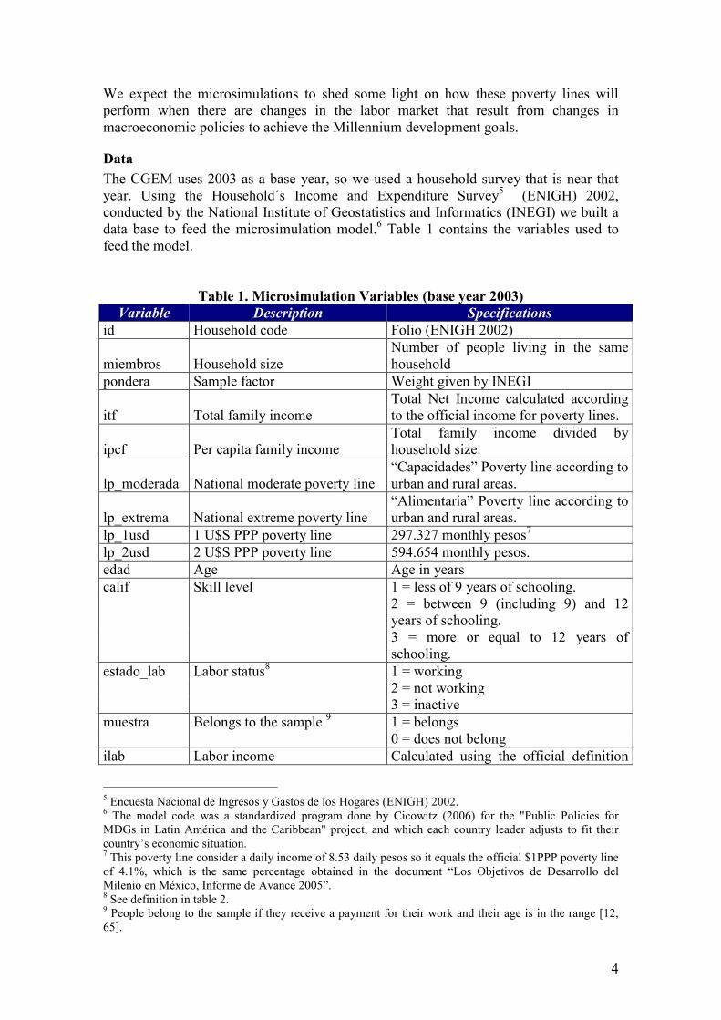
The CGEM uses 2003 as a base year, so we used a household survey that is near that year. Using the Household´s Income and Expenditure Survey5 (ENIGH) 2002, conducted by the National Institute of Geostatistics and Informatics (INEGI) we built a data base to feed the microsimulation model.6 Table 1 contains the variables used to feed the model.

Table 1. Microsimulation Variables (base year 2003)

Variable Description Specifications

id Household code Folio (ENIGH 2002)

miembros Household size Number of people living in the same household

pondera Sample factor Weight given by INEGI

itf Total family income Total Net Income calculated according to the official income for poverty lines.

ipcf Per capita family income Total family income divided by household size.

lp_moderada National moderate poverty line “Capacidades” Poverty line according to urban and rural areas.

lp_extrema National extreme poverty line “Alimentaria” Poverty line according to urban and rural areas.

lp_1usd 1 U$S PPP poverty line 297.327 monthly pesos7

lp_2usd 2 U$S PPP poverty line 594.654 monthly pesos.

edad Age Age in years

calif Skill level 1 = less of 9 years of schooling.

2 = between 9 (including 9) and 12 years of schooling.

3 = more or equal to 12 years of schooling.

estado_lab Labor status8 1 = working 2 = not working 3 = inactive

muestra Belongs to the sample 9 1 = belongs 0 = does not belong

ilab Labor income Calculated using the official definition

5 Encuesta Nacional de Ingresos y Gastos de los Hogares (ENIGH) 2002. 6 The model code was a standardized program done by Cicowitz (2006) for the "Public Policies for MDGs in Latin América and the Caribbean" project, and which each country leader adjusts to fit their country’s economic situation. 7 This poverty line consider a daily income of 8.53 daily pesos so it equals the official $1PPP poverty line of 4.1%, which is the same percentage obtained in the document “Los Objetivos de Desarrollo del Milenio en México, Informe de Avance 2005”. 8 See definition in table 2. 9 People belong to the sample if they receive a payment for their work and their age is in the range [12, 65].

5

in the poverty lines 2002

sector Economic sector of the worker 1: agriculture 2: manufacture 3: services 4: mining

grupoj group j of pertenece Skilled labor

grupok group k of pertenece Employment sector

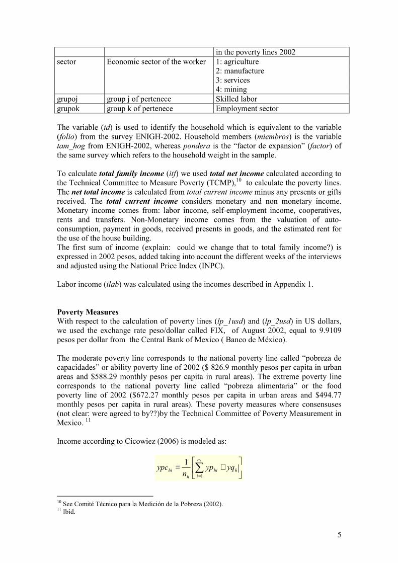
The variable (id) is used to identify the household which is equivalent to the variable (folio) from the survey ENIGH-2002. Household members (miembros) is the variable tam_hog from ENIGH-2002, whereas pondera is the “factor de expansion” (factor) of the same survey which refers to the household weight in the sample. To calculate total family income (itf) we used total net income calculated according to the Technical Committee to Measure Poverty (TCMP),10 to calculate the poverty lines. The net total income is calculated from total current income minus any presents or gifts received. The total current income considers monetary and non monetary income. Monetary income comes from: labor income, self-employment income, cooperatives, rents and transfers. Non-Monetary income comes from the valuation of auto-consumption, payment in goods, received presents in goods, and the estimated rent for the use of the house building. The first sum of income (explain: could we change that to total family income?) is expressed in 2002 pesos, added taking into account the different weeks of the interviews and adjusted using the National Price Index (INPC). Labor income (ilab) was calculated using the incomes described in Appendix 1.

Poverty Measures

With respect to the calculation of poverty lines (lp_1usd) and (lp_2usd) in US dollars, we used the exchange rate peso/dollar called FIX, of August 2002, equal to 9.9109 pesos per dollar from the Central Bank of Mexico ( Banco de México). The moderate poverty line corresponds to the national poverty line called “pobreza de capacidades” or ability poverty line of 2002 ($ 826.9 monthly pesos per capita in urban areas and $588.29 monthly pesos per capita in rural areas). The extreme poverty line corresponds to the national poverty line called “pobreza alimentaria” or the food poverty line of 2002 ($672.27 monthly pesos per capita in urban areas and $494.77 monthly pesos per capita in rural areas). These poverty measures where consensuses (not clear: were agreed to by??)by the Technical Committee of Poverty Measurement in Mexico. 11

Income according to Cicowiez (2006) is modeled as:

+= ∑

=h

n

i

hi

h

hi yqypn

ypch

1

1

10 See Comité Técnico para la Medición de la Pobreza (2002). 11 Ibid.

6

yphi = labor income per capita of household member i from household h, nh = household size h, yphi = labor income of household member i from household h,

yqh = sum of non-labor income

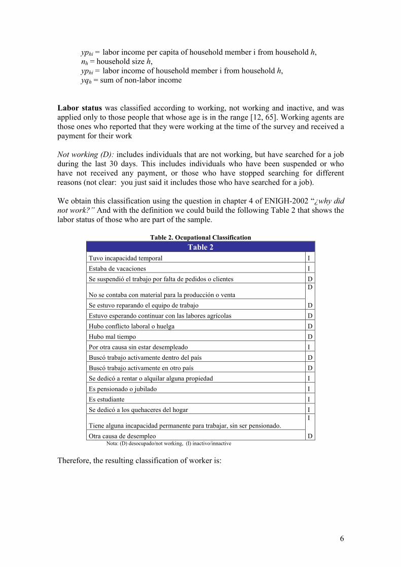
Labor status was classified according to working, not working and inactive, and was applied only to those people that whose age is in the range [12, 65]. Working agents are those ones who reported that they were working at the time of the survey and received a payment for their work �ot working (D): includes individuals that are not working, but have searched for a job during the last 30 days. This includes individuals who have been suspended or who have not received any payment, or those who have stopped searching for different reasons (not clear: you just said it includes those who have searched for a job). We obtain this classification using the question in chapter 4 of ENIGH-2002 “¿why did

not work?” And with the definition we could build the following Table 2 that shows the labor status of those who are part of the sample.

Table 2. Ocupational Classification

Table 2

Tuvo incapacidad temporal I

Estaba de vacaciones I

Se suspendió el trabajo por falta de pedidos o clientes D

No se contaba con material para la producción o venta D

Se estuvo reparando el equipo de trabajo D

Estuvo esperando continuar con las labores agrícolas D

Hubo conflicto laboral o huelga D

Hubo mal tiempo D

Por otra causa sin estar desempleado I

Buscó trabajo activamente dentro del país D

Buscó trabajo activamente en otro país D

Se dedicó a rentar o alquilar alguna propiedad I

Es pensionado o jubilado I

Es estudiante I

Se dedicó a los quehaceres del hogar I

Tiene alguna incapacidad permanente para trabajar, sin ser pensionado. I

Otra causa de desempleo D Nota: (D) desocupado/not working, (I) inactivo/innactive

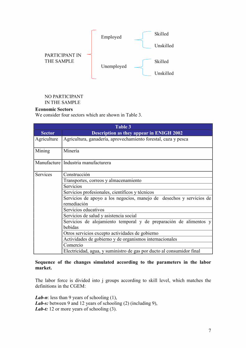
Therefore, the resulting classification of worker is:

7

PARTICIPANT IN

THE SAMPLE

NO PARTICIPANT

IN THE SAMPLE

Employed

Unemployed

Skilled

Unskilled

Skilled

Unskilled

Economic Sectors

We consider four sectors which are shown in Table 3.

Table 3

Sector Description as they appear in E1IGH 2002

Agriculture Agricultura, ganadería, aprovechamiento forestal, caza y pesca

Mining Minería

Manufacture Industria manufacturera

Services Construcción

Transportes, correos y almacenamiento

Servicios

Servicios profesionales, científicos y técnicos

Servicios de apoyo a los negocios, manejo de desechos y servicios de remediación

Servicios educativos

Servicios de salud y asistencia social

Servicios de alojamiento temporal y de preparación de alimentos y bebidas

Otros servicios excepto actividades de gobierno

Actividades de gobierno y de organismos internacionales

Comercio

Electricidad, agua, y suministro de gas por ducto al consumidor final

Sequence of the changes simulated according to the parameters in the labor

market.

The labor force is divided into j groups according to skill level, which matches the definitions in the CGEM: Lab-n: less than 9 years of schooling (1), Lab-s: between 9 and 12 years of schooling (2) (including 9), Lab-t: 12 or more years of schooling (3).

8

Then, the labor force is divided into k groups according to the economic sector they work in... 1: Agriculture 2: Mining 3: Manufacture 4: Services Given a labor market counterfactual we microsimulate the changes using the household survey.12 The parameters for simulating the changes of the labor market are defined as a function λ = λ (P,U,S,W1,W2,M):

P: labor participation rate for group j

U: unemployment rate of group j (skill level). S: employment structure for activity sector. W1: remuneration structure. W2: average level of remuneration. M: skilled structure of the employed labor force.

Effect S: employment structure for activity sector

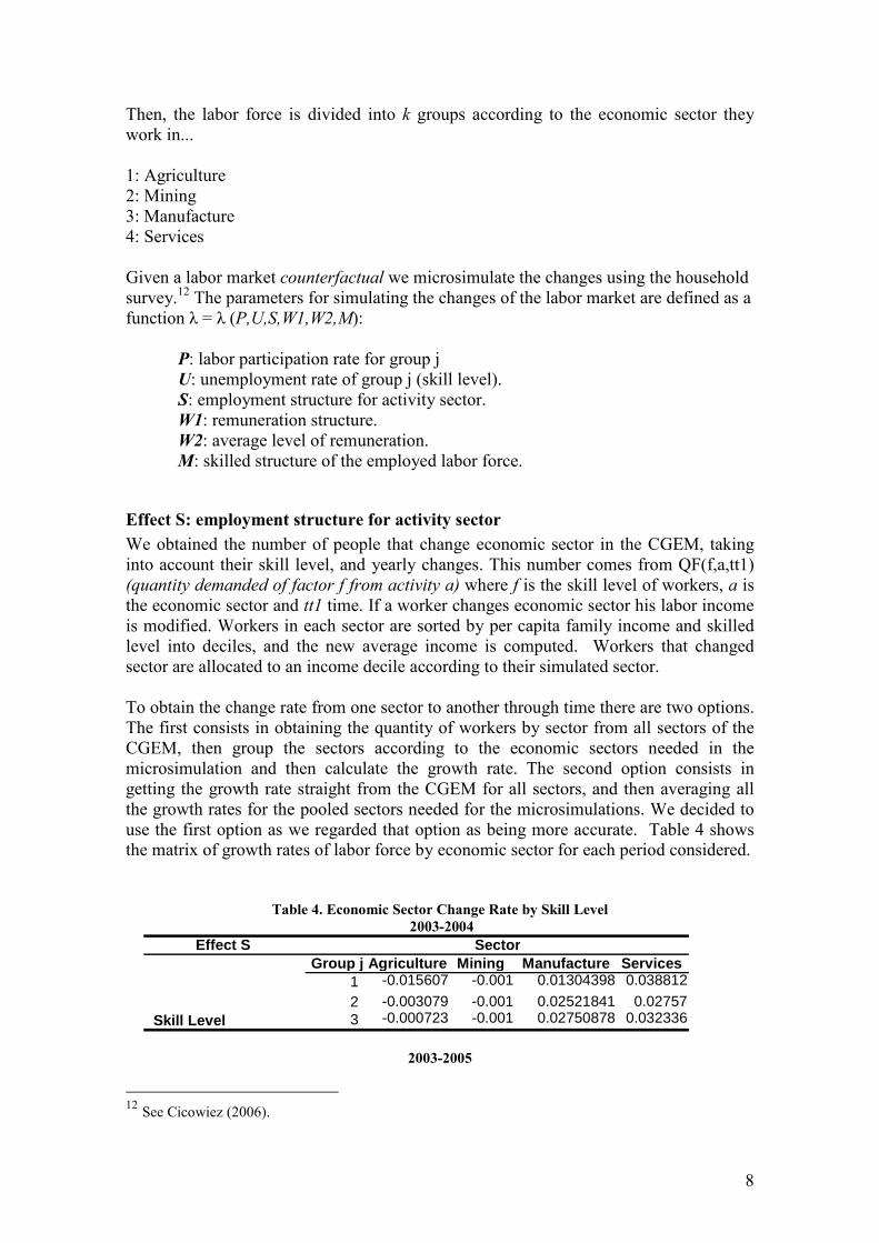
We obtained the number of people that change economic sector in the CGEM, taking into account their skill level, and yearly changes. This number comes from QF(f,a,tt1) (quantity demanded of factor f from activity a) where f is the skill level of workers, a is the economic sector and tt1 time. If a worker changes economic sector his labor income is modified. Workers in each sector are sorted by per capita family income and skilled level into deciles, and the new average income is computed. Workers that changed sector are allocated to an income decile according to their simulated sector. To obtain the change rate from one sector to another through time there are two options. The first consists in obtaining the quantity of workers by sector from all sectors of the CGEM, then group the sectors according to the economic sectors needed in the microsimulation and then calculate the growth rate. The second option consists in getting the growth rate straight from the CGEM for all sectors, and then averaging all the growth rates for the pooled sectors needed for the microsimulations. We decided to use the first option as we regarded that option as being more accurate. Table 4 shows the matrix of growth rates of labor force by economic sector for each period considered.

Table 4. Economic Sector Change Rate by Skill Level

2003-2004

2003-2005

12 See Cicowiez (2006).

Effect S Group j Agriculture Mining Manufacture Services

1 -0.015607 -0.001 0.01304398 0.038812

2 -0.003079 -0.001 0.02521841 0.027573 -0.000723 -0.001 0.02750878 0.032336

Sector

Skill Level

9

2003-2010

2003-2015

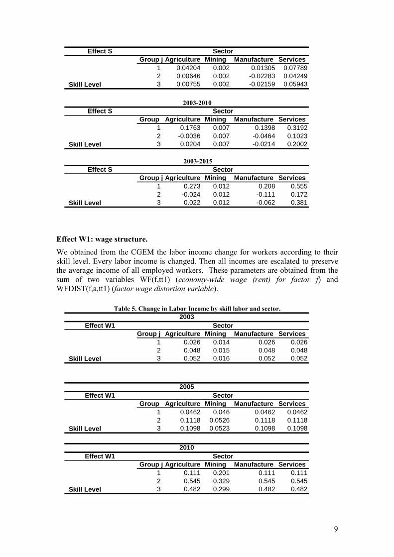
Effect W1: wage structure.

We obtained from the CGEM the labor income change for workers according to their skill level. Every labor income is changed. Then all incomes are escalated to preserve the average income of all employed workers. These parameters are obtained from the sum of two variables WF(f,tt1) (economy-wide wage (rent) for factor f) and WFDIST(f,a,tt1) (factor wage distortion variable).

Table 5. Change in Labor Income by skill labor and sector.

Effect W1Group j Agriculture Mining Manufacture Services

1 0.111 0.201 0.111 0.1112 0.545 0.329 0.545 0.5453 0.482 0.299 0.482 0.482

Sector

Skill Level

2010

Effect W1Group Agriculture Mining Manufacture Services

1 0.0462 0.046 0.0462 0.04622 0.1118 0.0526 0.1118 0.11183 0.1098 0.0523 0.1098 0.1098

2005 Sector

Skill Level

Effect W1Group j Agriculture Mining Manufacture Services

1 0.026 0.014 0.026 0.0262 0.048 0.015 0.048 0.0483 0.052 0.016 0.052 0.052

2003 Sector

Skill Level

Effect S Group j Agriculture Mining Manufacture Services

1 0.273 0.012 0.208 0.5552 -0.024 0.012 -0.111 0.1723 0.022 0.012 -0.062 0.381Skill Level

Sector

Effect S Group Agriculture Mining Manufacture Services

1 0.1763 0.007 0.1398 0.31922 -0.0036 0.007 -0.0464 0.10233 0.0204 0.007 -0.0214 0.2002

Sector

Skill Level

Effect S Group j Agriculture Mining Manufacture Services

1 0.04204 0.002 0.01305 0.077892 0.00646 0.002 -0.02283 0.042493 0.00755 0.002 -0.02159 0.05943Skill Level

Sector

10

Effect: Average Wage

Labor income is multiplied by the average increase in labor income from the CGEM for each period considered. To perform this multiplication it is necessary to average all incomes by period.

Table 6. Average Labor Growth Rate W2

Año Incremento en el salario2003 0.04862005 0.10302010 0.45242015 0.9170

Efecto W2

Effect: Change in Skill level

We obtain from the CGE the change rate from one skilled level to another by sector. The parameters come from the variable QF(f,a,tt1) (quantity demanded of factor f from

activity a). This change matrix is the transpose matrix of effect s (see Table 4).

Poverty and Inequality Measures

The following poverty and inequality measures are calculated after applying all the effects to the labor force: fgt_1usd: percentage of agents below the poverty line of 1us dollar PPP a day. fgt_2usd: percentage of agents below the poverty line of 2 us dollars PPP a day. fgt_moderada: percentage of agents below the poverty line called de capacidades. fgt_extrema: percentage of agents below the poverty line called alimentaria. gini_ipcf: gini index of per capita family income. gini_ilab: gini index of labor income. mean_ilab: average labor income for all simulated effects. mean_ipfc: average per capita family income for all simulated effects.

Methodology

The microsimulation is performed using stata (Explain). In this way we obtain the data base of agents from the household survey. Using the CGEM changing rates described in Tables 4 to 6, we model some effects of Ganuza et al. (2002), such that every participing worker is allocated a random number in the data base. Next, workers are sorted by economic sector and skill level, and then workers are assigned income according to the new λ* and can be employed or unemployed. If they became

Effect W1Group j Agriculture Mining Manuf acture Services

1 0.20702 0.33633 0.20702 0.207022 1.13946 0.77658 1.13946 1.139463 0.97814 0.66722 0.97814 0.97814Skill Level

2015 Sector

11

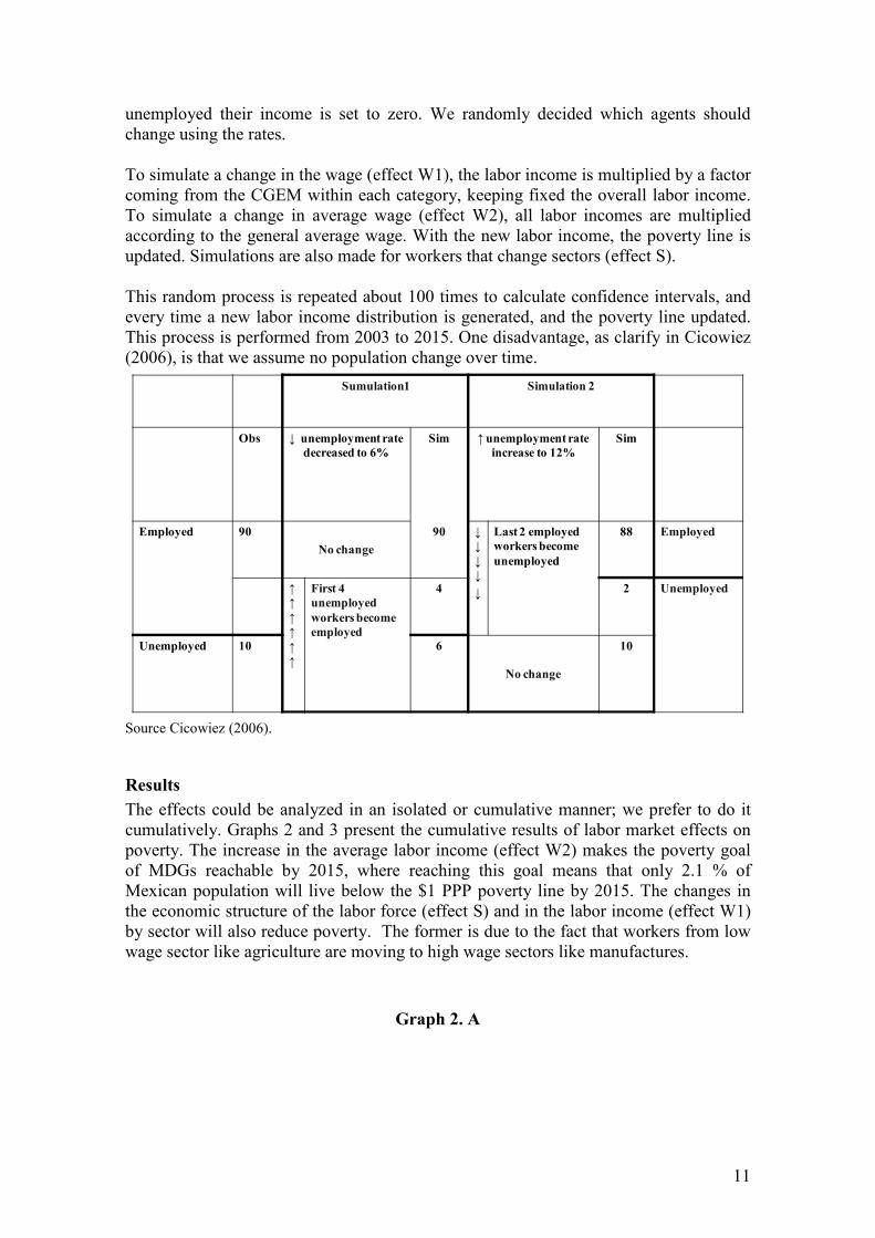
unemployed their income is set to zero. We randomly decided which agents should change using the rates. To simulate a change in the wage (effect W1), the labor income is multiplied by a factor coming from the CGEM within each category, keeping fixed the overall labor income. To simulate a change in average wage (effect W2), all labor incomes are multiplied according to the general average wage. With the new labor income, the poverty line is updated. Simulations are also made for workers that change sectors (effect S). This random process is repeated about 100 times to calculate confidence intervals, and every time a new labor income distribution is generated, and the poverty line updated. This process is performed from 2003 to 2015. One disadvantage, as clarify in Cicowiez (2006), is that we assume no population change over time.

Sumulation1 Simulation 2

Obs ↓ unemployment rate

decreased to 6%

Sim ↑ unemployment rate

increase to 12%

Sim

Employed 90

1o change

90 ↓

↓

↓

↓

↓

Last 2 employed

workers become

unemployed

88 Employed

↑

↑

↑

↑

↑

↑

First 4

unemployed

workers become

employed

4 2 Unemployed

Unemployed 10 6

1o change

10

Source Cicowiez (2006).

Results

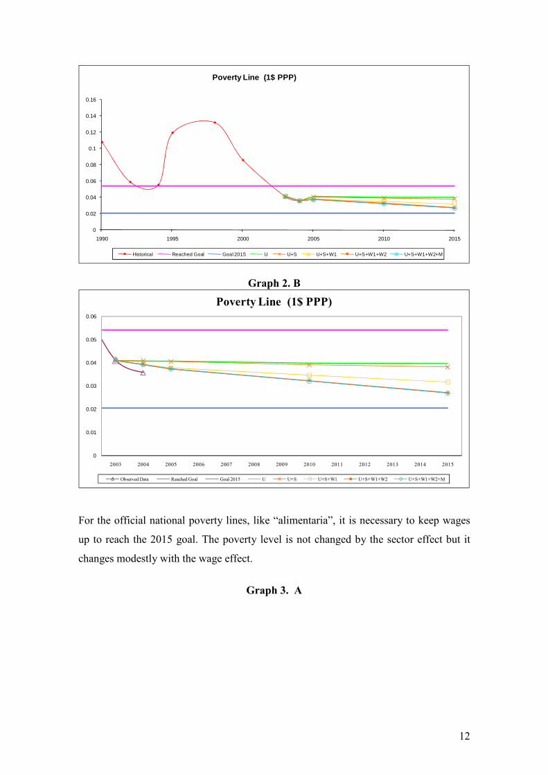
The effects could be analyzed in an isolated or cumulative manner; we prefer to do it cumulatively. Graphs 2 and 3 present the cumulative results of labor market effects on poverty. The increase in the average labor income (effect W2) makes the poverty goal of MDGs reachable by 2015, where reaching this goal means that only 2.1 % of Mexican population will live below the $1 PPP poverty line by 2015. The changes in the economic structure of the labor force (effect S) and in the labor income (effect W1) by sector will also reduce poverty. The former is due to the fact that workers from low wage sector like agriculture are moving to high wage sectors like manufactures.

Graph 2. A

12

0

0.02

0.04

0.06

0.08

0.1

0.12

0.14

0.16

1990 1995 2000 2005 2010 2015

Poverty Line (1$ PPP)

Historical Reached Goal Goal 2015 U U+S U+S+W1 U+S+W1+W2 U+S+W1+W2+M

Graph 2. B

0

0.01

0.02

0.03

0.04

0.05

0.06

2003 2004 2005 2006 2007 2008 2009 2010 2011 2012 2013 2014 2015

Poverty Line (1$ PPP)

Observed Data Reached Goal Goal 2015 U U+S U+S+W1 U+S+W1+W2 U+S+W1+W2+M

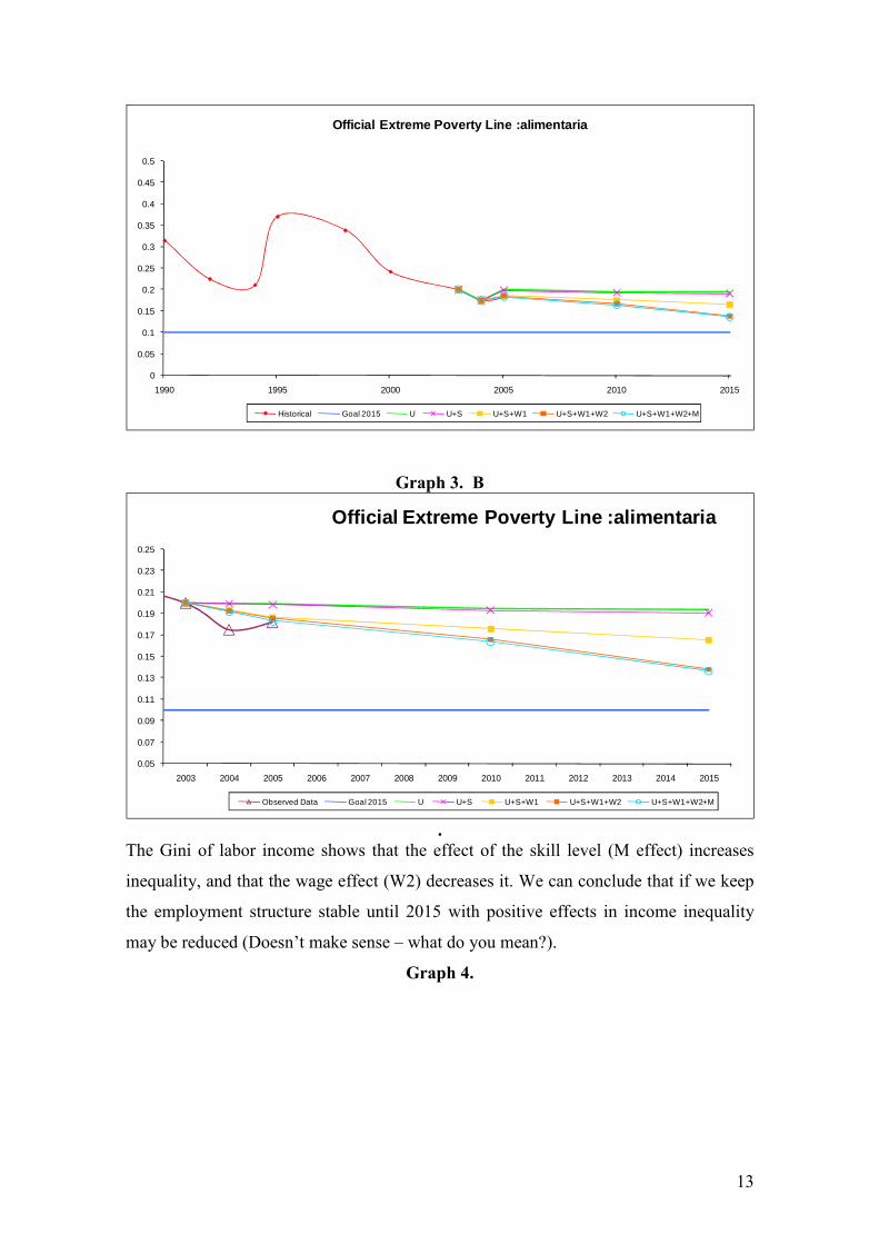
For the official national poverty lines, like “alimentaria”, it is necessary to keep wages

up to reach the 2015 goal. The poverty level is not changed by the sector effect but it

changes modestly with the wage effect.

Graph 3. A

13

0

0.05

0.1

0.15

0.2

0.25

0.3

0.35

0.4

0.45

0.5

1990 1995 2000 2005 2010 2015

Official Extreme Poverty Line :alimentaria

Historical Goal 2015 U U+S U+S+W1 U+S+W1+W2 U+S+W1+W2+M

Graph 3. B

0.05

0.07

0.09

0.11

0.13

0.15

0.17

0.19

0.21

0.23

0.25

2003 2004 2005 2006 2007 2008 2009 2010 2011 2012 2013 2014 2015

Official Extreme Poverty Line :alimentaria

Observed Data Goal 2015 U U+S U+S+W1 U+S+W1+W2 U+S+W1+W2+M

.

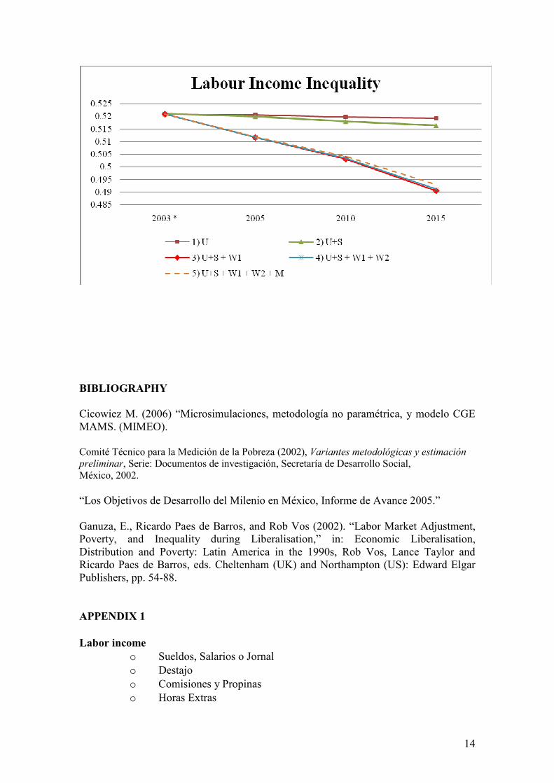
The Gini of labor income shows that the effect of the skill level (M effect) increases

inequality, and that the wage effect (W2) decreases it. We can conclude that if we keep

the employment structure stable until 2015 with positive effects in income inequality

may be reduced (Doesn’t make sense – what do you mean?).

Graph 4.

14

BIBLIOGRAPHY

Cicowiez M. (2006) “Microsimulaciones, metodología no paramétrica, y modelo CGE MAMS. (MIMEO). Comité Técnico para la Medición de la Pobreza (2002), Variantes metodológicas y estimación

preliminar, Serie: Documentos de investigación, Secretaría de Desarrollo Social, México, 2002.

“Los Objetivos de Desarrollo del Milenio en México, Informe de Avance 2005.” Ganuza, E., Ricardo Paes de Barros, and Rob Vos (2002). “Labor Market Adjustment, Poverty, and Inequality during Liberalisation,” in: Economic Liberalisation, Distribution and Poverty: Latin America in the 1990s, Rob Vos, Lance Taylor and Ricardo Paes de Barros, eds. Cheltenham (UK) and Northampton (US): Edward Elgar Publishers, pp. 54-88.

APPE1DIX 1

Labor income

o Sueldos, Salarios o Jornal

o Destajo

o Comisiones y Propinas

o Horas Extras

15

o Aguinaldo

o Incentivos, Gratificaciones o Premios

o Bono, Percepción Adicional o Sobresueldo

o Primas Vacacionales y Otras Prestaciones en Efectivo

o Reparto de Utilidades

Self-Employment Income

o Negocios Industriales

o Negocios Comerciales

o Prestación de Servicios

o Producción Agrícola

o Cría, explotación y productos derivados de animales

o Reproducción, corte y tala de árboles

o Recolección de Flora, Productos Forestales Caza captura de animales

o Cría y explotación de plantas y animales acuáticos y pesca

Cooperative Income

o Sueldos o Salarios

Societies Income

o Sueldos, salarios o jornal

Societies “like” Income

o sueldos, salarios o jornal

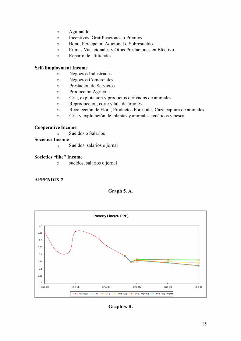
APPE1DIX 2

Graph 5. A.

0

0.05

0.1

0.15

0.2

0.25

0.3

0.35

0.4

Ene-90 Ene-95 Ene-00 Ene-05 Ene-10 Ene-15

Poverty Line(2$ PPP)

Historical U U+S U+S+W1 U+S+W1+W2 U+S+W1+W2+M

Graph 5. B.

16

0.09

0.14

0.19

0.24

2003 2004 2005 2006 2007 2008 2009 2010 2011 2012 2013 2014 2015

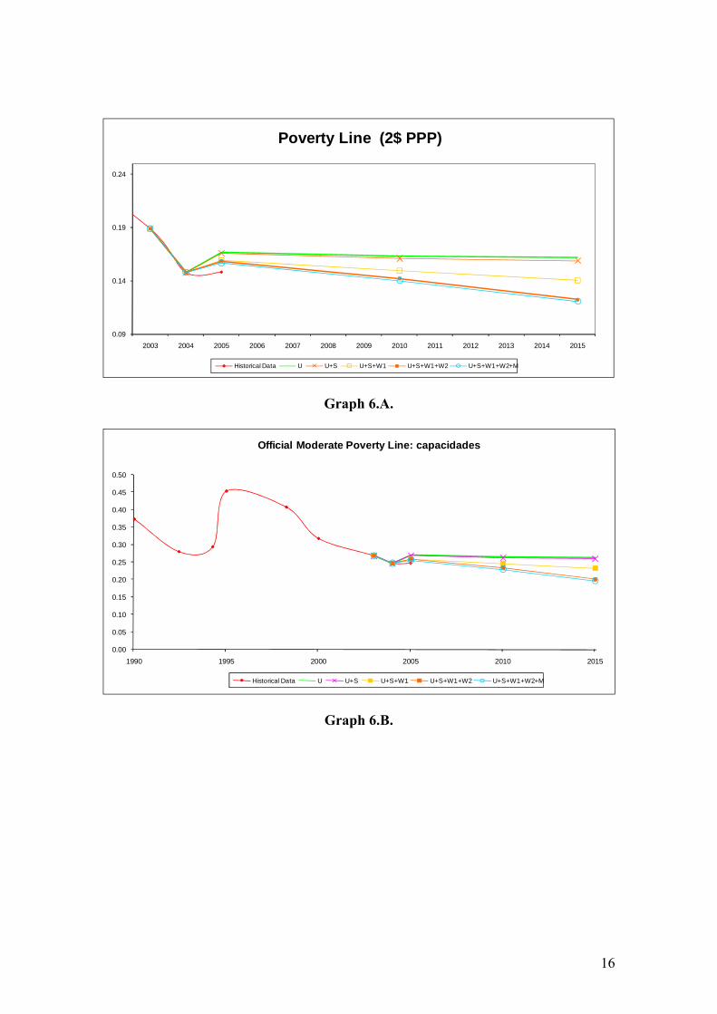
Poverty Line (2$ PPP)

Historical Data U U+S U+S+W1 U+S+W1+W2 U+S+W1+W2+M

Graph 6.A.

0.00

0.05

0.10

0.15

0.20

0.25

0.30

0.35

0.40

0.45

0.50

1990 1995 2000 2005 2010 2015

Official Moderate Poverty Line: capacidades

Historical Data U U+S U+S+W1 U+S+W1+W2 U+S+W1+W2+M

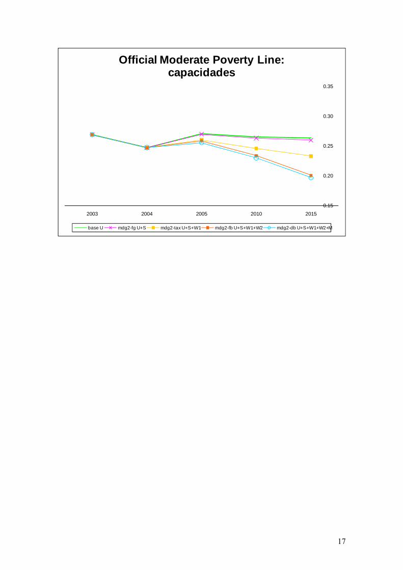
Graph 6.B.

17

0.15

0.20

0.25

0.30

0.35

2003 2004 2005 2010 2015

Official Moderate Poverty Line: capacidades

base U mdg2-fg U+S mdg2-tax U+S+W1 mdg2-fb U+S+W1+W2 mdg2-db U+S+W1+W2+M