Embed Size (px)
Citation preview
1
Digital Audio Signal Processing
Lecture-2
Microphone Array Processing
Marc Moonen Dept. E.E./ESAT-STADIUS, KU Leuven
[email protected] homes.esat.kuleuven.be/~moonen/
Digital Audio Signal Processing Version 2015-2016 Lecture-2: Microphone Array Processing p. 2
Overview
• Introduction & beamforming basics – Data model & definitions
• Fixed beamforming – Filter-and-sum beamformer design – Matched filtering
• White noise gain maximization • Ex: Delay-and-sum beamforming
– Superdirective beamforming • Directivity maximization
– Directional microphones (delay-and-subtract)
• Adaptive Beamforming – LCMV beamformer – Generalized sidelobe canceler
2
Digital Audio Signal Processing Version 2015-2016 Lecture-2: Microphone Array Processing p. 3
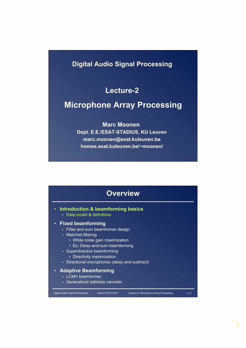
Introduction
• Directivity pattern of a microphone – A microphone (*) is characterized by a `directivity pattern which specifies the gain & phase shift that the microphone gives to a signal coming from a certain direction (i.e. `angle-of-arrival’) – In general the directivity pattern is a function of frequency (ω) – In a 3D scenario `angle-of-arrival’ is azimuth + elevation angle – Will consider only 2D scenarios for simplicity, with one angle-of arrival (θ), hence directivity pattern is H(ω,θ) – Directivity pattern is fixed and defined by physical microphone design
(*) We do digital signal prcessing, so this includes front-end filtering/A-to-D/..
|H(ω,θ)| for 1 frequency
Digital Audio Signal Processing Version 2015-2016 Lecture-2: Microphone Array Processing p. 4
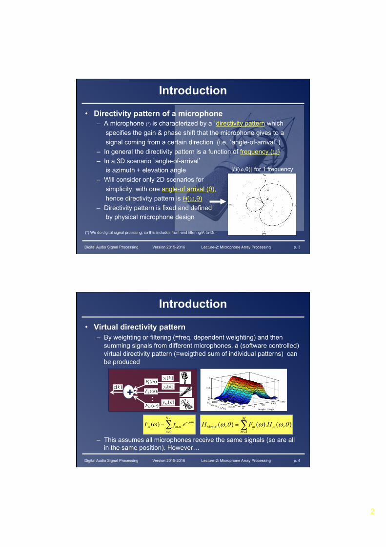
Introduction
• Virtual directivity pattern – By weighting or filtering (=freq. dependent weighting) and then
summing signals from different microphones, a (software controlled) virtual directivity pattern (=weigthed sum of individual patterns) can be produced
– This assumes all microphones receive the same signals (so are all in the same position). However…
∑=
=M
mmm HFH
1virtual ),().(),( θωωθω
01000
20003000 0
4590
135180
0
0.5
1
Angle (deg)
Frequency (Hz)
F1(ω)
F2 (ω)
FM (ω)
z[k]
y1[k]
y2[k]
yM [k]
+ :
Fm (ω) = fm,n.e− jωn
n=0
N−1
∑
3
Digital Audio Signal Processing Version 2015-2016 Lecture-2: Microphone Array Processing p. 5
F1(ω)
F2 (ω)
FM (ω)
z[k]
y1[k]
+ : dM
θ
dM cosθ
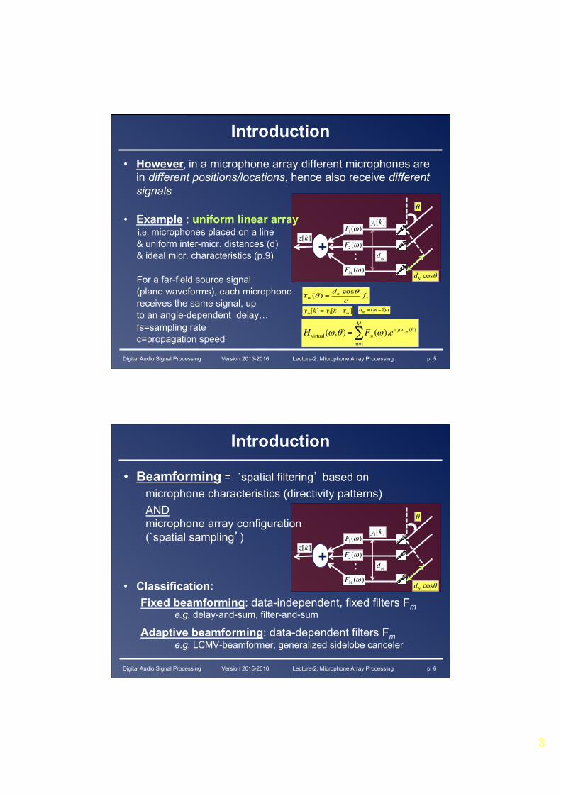
Introduction
• However, in a microphone array different microphones are in different positions/locations, hence also receive different signals
• Example : uniform linear array i.e. microphones placed on a line & uniform inter-micr. distances (d) & ideal micr. characteristics (p.9) For a far-field source signal (plane waveforms), each microphone receives the same signal, up to an angle-dependent delay… fs=sampling rate c=propagation speed
][][ 1 mm kyky τ+=
Hvirtual (ω,θ ) = Fm (ω).e− jωτm (θ )
m=1
M
∑
sm
m fc
d θθτ
cos)( =
dmdm )1( −=
Digital Audio Signal Processing Version 2015-2016 Lecture-2: Microphone Array Processing p. 6
F1(ω)
F2 (ω)
FM (ω)
z[k]
y1[k]
+ : dM
θ
dM cosθ
Introduction
• Beamforming = `spatial filtering’ based on microphone characteristics (directivity patterns) AND microphone array configuration (`spatial sampling’)
• Classification: Fixed beamforming: data-independent, fixed filters Fm e.g. delay-and-sum, filter-and-sum
Adaptive beamforming: data-dependent filters Fm e.g. LCMV-beamformer, generalized sidelobe canceler
4
Digital Audio Signal Processing Version 2015-2016 Lecture-2: Microphone Array Processing p. 7
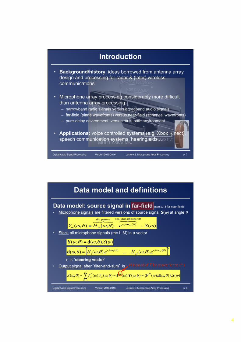
Introduction
• Background/history: ideas borrowed from antenna array design and processing for radar & (later) wireless communications
• Microphone array processing considerably more difficult than antenna array processing: – narrowband radio signals versus broadband audio signals – far-field (plane wavefronts) versus near-field (spherical wavefronts) – pure-delay environment versus multi-path environment
• Applications: voice controlled systems (e.g. Xbox Kinect), speech communication systems, hearing aids,…
Digital Audio Signal Processing Version 2015-2016 Lecture-2: Microphone Array Processing p. 8
Data model and definitions
Data model: source signal in far-field (see p.13 for near-field)
• Microphone signals are filtered versions of source signal S(ω) at angle θ
• Stack all microphone signals (m=1..M) in a vector d is `steering vector’ • Output signal after `filter-and-sum’ is
[ ]TjM
j MeHeH )()(1 ).,(...).,(),( 1 θωτθωτ θωθωθω −−=d
)()}.,().({),().(),().(),(1
* ωθωωθωωθωωθω SYFZ HHM
mmm dFYF ===∑
=
H instead of T for convenience (**)
)( ..),(),(shift phase dep.-pos.
)(
pattern dir.
ωθωθω θωτ SeHY mjmm
!"!#$!"!#$−=
)().,(),( ωθωθω SdY =
5
Digital Audio Signal Processing Version 2015-2016 Lecture-2: Microphone Array Processing p. 9
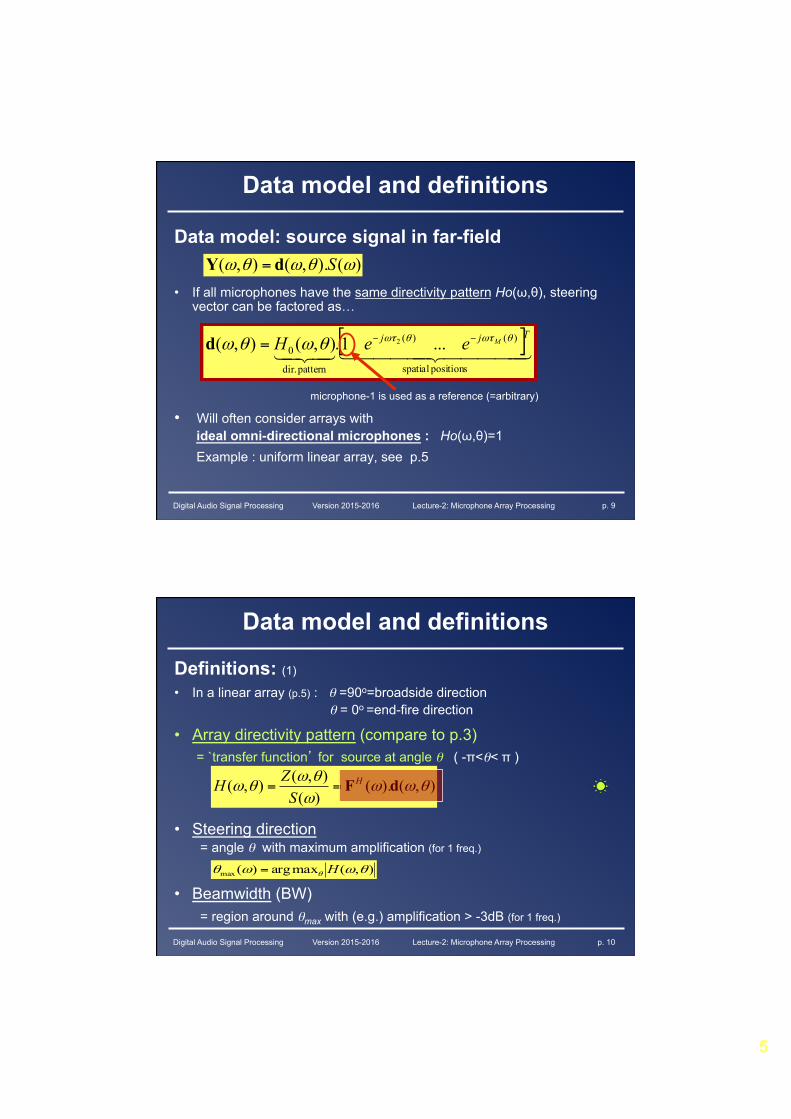
Data model: source signal in far-field • If all microphones have the same directivity pattern Ho(ω,θ), steering
vector can be factored as…
• Will often consider arrays with ideal omni-directional microphones : Ho(ω,θ)=1 Example : uniform linear array, see p.5
Data model and definitions
)().,(),( ωθωθω SdY =
[ ]!!!!! "!!!!! #$!"!#$positions spatial
)()(
pattern dir.
0 ...1.),(),( 2Tjj MeeH θωτθωτθωθω −−=d
microphone-1 is used as a reference (=arbitrary)
Digital Audio Signal Processing Version 2015-2016 Lecture-2: Microphone Array Processing p. 10
Data model and definitions
Definitions: (1) • In a linear array (p.5) : θ =90o=broadside direction θ = 0o =end-fire direction
• Array directivity pattern (compare to p.3) = `transfer function’ for source at angle θ ( -π<θ< π )
• Steering direction = angle θ with maximum amplification (for 1 freq.)
• Beamwidth (BW) = region around θmax with (e.g.) amplification > -3dB (for 1 freq.)
),().()(),(),( θωω
ωθω
θω dFHSZH ==
),(maxarg)(max θωωθ θ H=
6
Digital Audio Signal Processing Version 2015-2016 Lecture-2: Microphone Array Processing p. 11
Data model and definitions
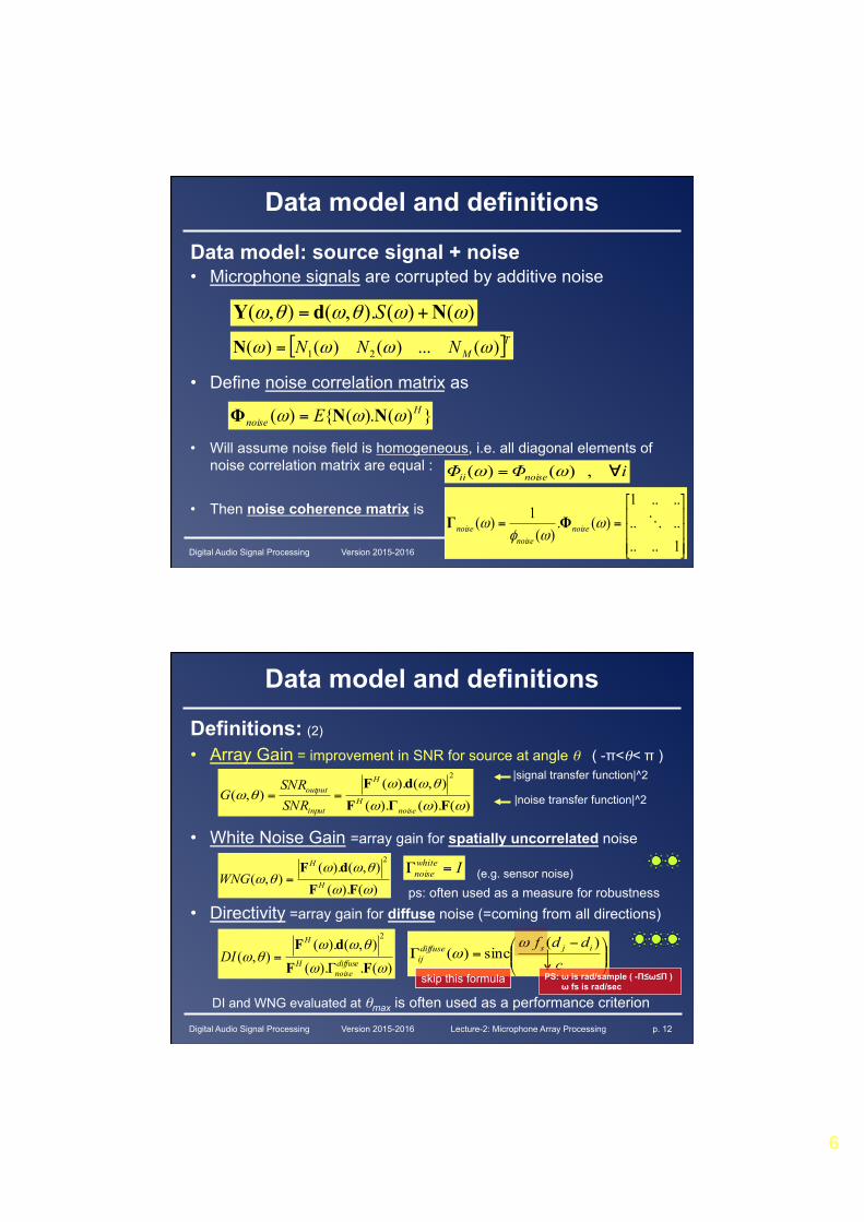
Data model: source signal + noise • Microphone signals are corrupted by additive noise
• Define noise correlation matrix as
• Will assume noise field is homogeneous, i.e. all diagonal elements of noise correlation matrix are equal :
• Then noise coherence matrix is
[ ]TMNNN )(...)()()( 21 ωωωω =N
})().({)( Hnoise E ωωω NNΦ =
iΦΦ noiseii ∀= , )()( ωω
⎥⎥⎥
⎦
⎤
⎢⎢⎢
⎣
⎡
==
1............1
)(.)(
1)( !ωωφ
ω noisenoise
noise ΦΓ
)()().,(),( ωωθωθω NdY += S
Digital Audio Signal Processing Version 2015-2016 Lecture-2: Microphone Array Processing p. 12
Data model and definitions
Definitions: (2) • Array Gain = improvement in SNR for source at angle θ ( -π<θ< π )
• White Noise Gain =array gain for spatially uncorrelated noise
(e.g. sensor noise) ps: often used as a measure for robustness • Directivity =array gain for diffuse noise (=coming from all directions)
DI and WNG evaluated at θmax is often used as a performance criterion
⎟⎟⎠
⎞⎜⎜⎝
⎛ −=Γ
cddf ijsdiffuse
ij
)(sinc)(
ωω
skip this formula )(.).(
),().(),(
2
ωω
θωωθω
FFdFdiffusenoise
H
H
DIΓ
=
)().(),().(
),(2
ωω
θωωθω
FFdF
H
H
WNG =Iwhite
noise =Γ
|signal transfer function|^2
|noise transfer function|^2 )().().(),().(
),(2
ωωω
θωωθω
FΓFdF
noiseH
H
input
output
SNRSNR
G ==
PS: ω is rad/sample ( -Π≤ω≤Π ) ω fs is rad/sec
7
Digital Audio Signal Processing Version 2015-2016 Lecture-2: Microphone Array Processing p. 13
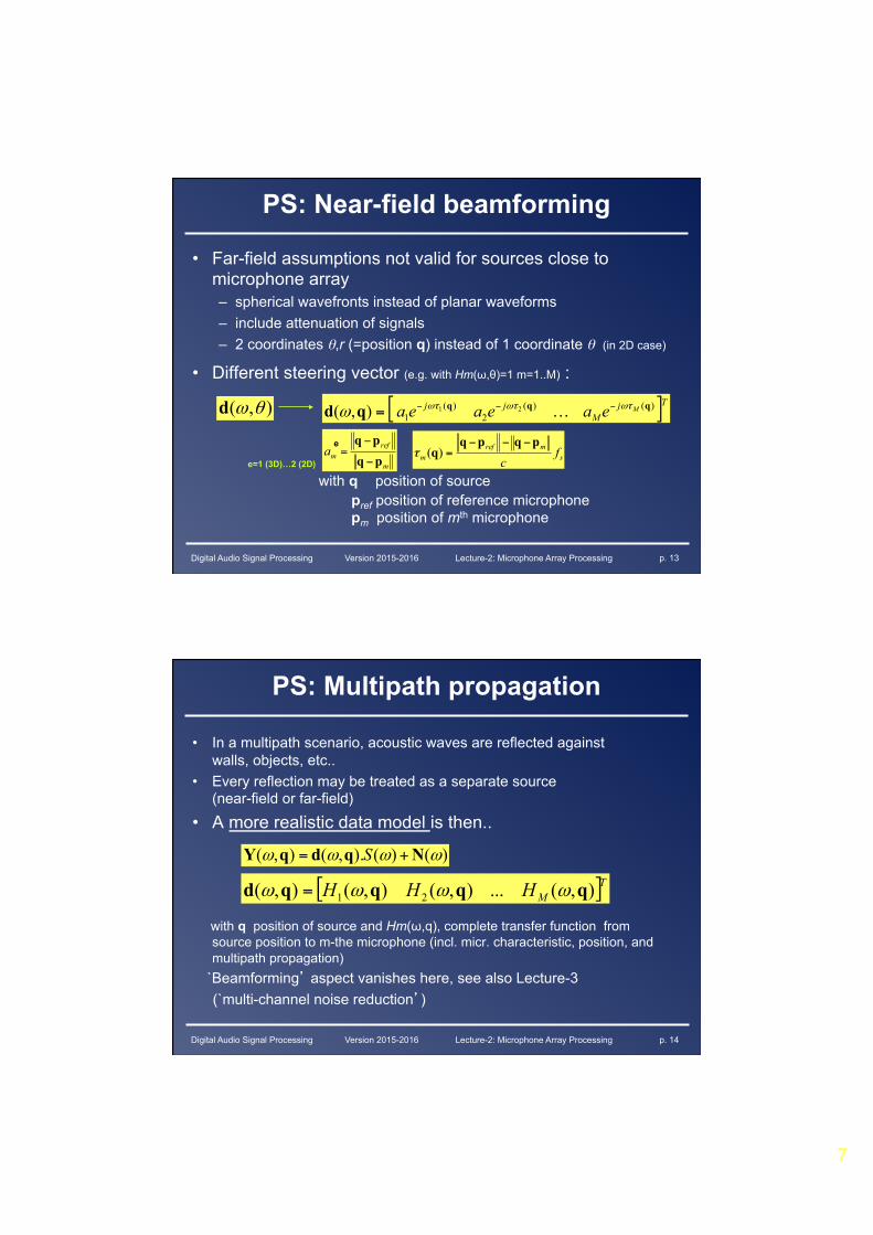
• Far-field assumptions not valid for sources close to microphone array – spherical wavefronts instead of planar waveforms – include attenuation of signals – 2 coordinates θ,r (=position q) instead of 1 coordinate θ (in 2D case)
• Different steering vector (e.g. with Hm(ω,θ)=1 m=1..M) :
PS: Near-field beamforming
[ ]TjM
jj Meaeaea )()(2
)(1
21),( qqqqd ωτωτωτω −−−= …),( θωd
smref
m fc
pqpqq
−−−=)(τ
with q position of source pref position of reference microphone pm position of mth microphone
m
refma pq
pq−
−=
e
e=1 (3D)…2 (2D)
Digital Audio Signal Processing Version 2015-2016 Lecture-2: Microphone Array Processing p. 14
PS: Multipath propagation
• In a multipath scenario, acoustic waves are reflected against walls, objects, etc..
• Every reflection may be treated as a separate source (near-field or far-field)
• A more realistic data model is then.. with q position of source and Hm(ω,q), complete transfer function from
source position to m-the microphone (incl. micr. characteristic, position, and multipath propagation)
`Beamforming’ aspect vanishes here, see also Lecture-3 (`multi-channel noise reduction’)
)()().,(),( ωωωω NqdqY += S
[ ]TMHHH ),(...),(),(),( 21 qqqqd ωωωω =
8
Digital Audio Signal Processing Version 2015-2016 Lecture-2: Microphone Array Processing p. 15
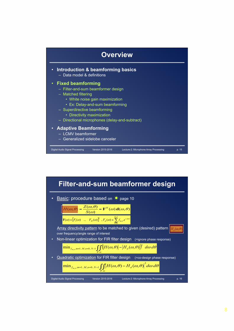
Overview
• Introduction & beamforming basics – Data model & definitions
• Fixed beamforming – Filter-and-sum beamformer design – Matched filtering
• White noise gain maximization • Ex: Delay-and-sum beamforming
– Superdirective beamforming • Directivity maximization
– Directional microphones (delay-and-subtract)
• Adaptive Beamforming – LCMV beamformer – Generalized sidelobe canceler
Digital Audio Signal Processing Version 2015-2016 Lecture-2: Microphone Array Processing p. 16
Filter-and-sum beamformer design
• Basic: procedure based on page 10 Array directivity pattern to be matched to given (desired) pattern over frequency/angle range of interest
• Non-linear optimization for FIR filter design (=ignore phase response)
• Quadratic optimization for FIR filter design (=co-design phase response)
),().()(),(),( θωω
ωθω
θω dFHSZH ==
),( θωdH
[ ] ∑−
=
−==1
0,1 .)( , )(...)()(
N
n
jnnmm
TM efFFF ωωωωωF
θωθωθωθ ω
ddHH dNnMmf nm ),(),(min
2
1..0,..1,, ∫ ∫ −−==
( ) θωθωθωθ ω
ddHH dNnMmf nm ),(),(min 2
1..0,..1,, ∫ ∫ −−==
9
Digital Audio Signal Processing Version 2015-2016 Lecture-2: Microphone Array Processing p. 17
Filter-and-sum beamformer design • Quadratic optimization for FIR filter design (continued)
With optimal solution is
θωθωθωθ ω
ddHH dNnMmf nm ),(),(min
2
1..0,..1,, ∫ ∫ −−==
[ ] [ ]
[ ]!!!! "!!!! #$
!!! %!!! &'
(
),(
).1(
.0
1
11,0,
),(.)(.),(.)(...)(),().(),(
... , ...
θω
ω
ω
θωθωωωθωωθω
d
dfddF
ffffNMxM
jN
j
MxMTH
MHH
TTM
TTNmmm
e
eIFFH
ff
⎥⎥⎥
⎦
⎤
⎢⎢⎢
⎣
⎡
⊗===
==
−
−
∫ ∫∫ ∫ === −
θ ωθ ωθωθωθωθωθωθω ddHdd d
Hoptimal ),().,( , ),().,( , . *1 dpddQpQf
Kronecker product
Digital Audio Signal Processing Version 2015-2016 Lecture-2: Microphone Array Processing p. 18
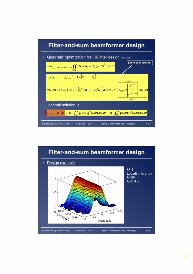
Filter-and-sum beamformer design • Design example
M=8 Logarithmic array N=50 fs=8 kHz
01000
20003000 0
4590
135180
0
0.5
1
Angle (deg)
Frequency (Hz)
10
Digital Audio Signal Processing Version 2015-2016 Lecture-2: Microphone Array Processing p. 19
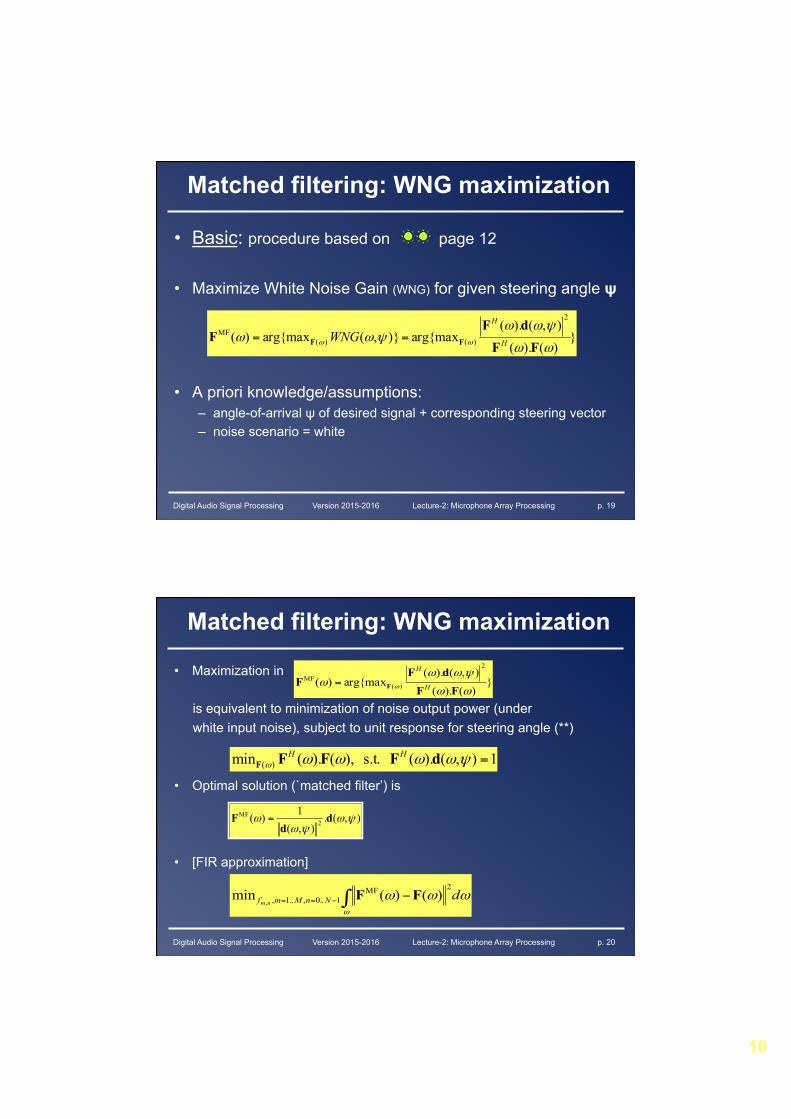
Matched filtering: WNG maximization
• Basic: procedure based on page 12
• Maximize White Noise Gain (WNG) for given steering angle ψ
• A priori knowledge/assumptions: – angle-of-arrival ψ of desired signal + corresponding steering vector – noise scenario = white
})().(),().(
arg{max)},(arg{max)(2
)()(MF
ωω
ψωωψωω ωω FF
dFF FF H
H
WNG ==
Digital Audio Signal Processing Version 2015-2016 Lecture-2: Microphone Array Processing p. 20
Matched filtering: WNG maximization
• Maximization in is equivalent to minimization of noise output power (under white input noise), subject to unit response for steering angle (**)
• Optimal solution (`matched filter’) is
• [FIR approximation]
),(.),(
1)( 2MF ψω
ψωω d
dF =
1),().( s.t. ),().(min )( =ψωωωωω dFFFFHH
})().(),().(
arg{max)(2
)(MF
ωω
ψωωω ω FF
dFF F H
H
=
ωωωω
dNnMmf nm ∫ −−==
2MF1..0,..1, )()(min
,FF
11
Digital Audio Signal Processing Version 2015-2016 Lecture-2: Microphone Array Processing p. 21
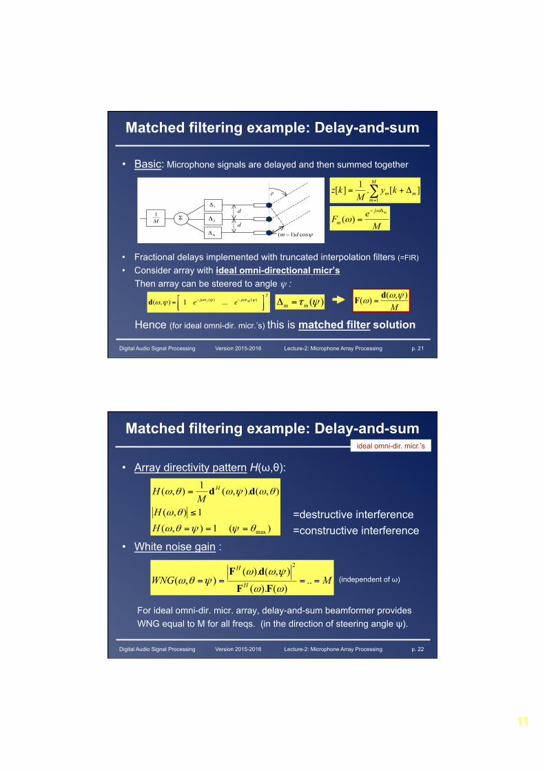
Matched filtering example: Delay-and-sum
• Basic: Microphone signals are delayed and then summed together
• Fractional delays implemented with truncated interpolation filters (=FIR)
• Consider array with ideal omni-directional micr’s Then array can be steered to angle ψ :
Hence (for ideal omni-dir. micr.’s) this is matched filter solution
1),( =ψωH
d
ψcos)1( dm −
Σ d
2Δ mΔ
1Δ
M1
ψ
MeF
mj
m
Δ−
=ω
ω)(
∑=
Δ+=M
mmm ky
Mkz
1
][.1][
d(ω,ψ) = 1 e− jωτ 2 (ψ ) ... e− jωτM (ψ )"#$
%&'
T
)(ψτmm =Δ M),()( ψω
ωdF =
Digital Audio Signal Processing Version 2015-2016 Lecture-2: Microphone Array Processing p. 22
Matched filtering example: Delay-and-sum
• Array directivity pattern H(ω,θ):
=destructive interference =constructive interference • White noise gain :
(independent of ω)
For ideal omni-dir. micr. array, delay-and-sum beamformer provides WNG equal to M for all freqs. (in the direction of steering angle ψ).
)( 1),(1),(
),().,(1),(
maxθψψθω
θω
θωψωθω
===
≤
=
HH
MH H dd
MWNG H
H
==== ..)().(),().(
),(2
ωω
ψωωψθω
FFdF
ideal omni-dir. micr.’s
12
Digital Audio Signal Processing Version 2015-2016 Lecture-2: Microphone Array Processing p. 23
02000
40006000
8000 045 90 135
180
0.2
0.4
0.6
0.8
1
Angle (deg)Frequency (Hz)
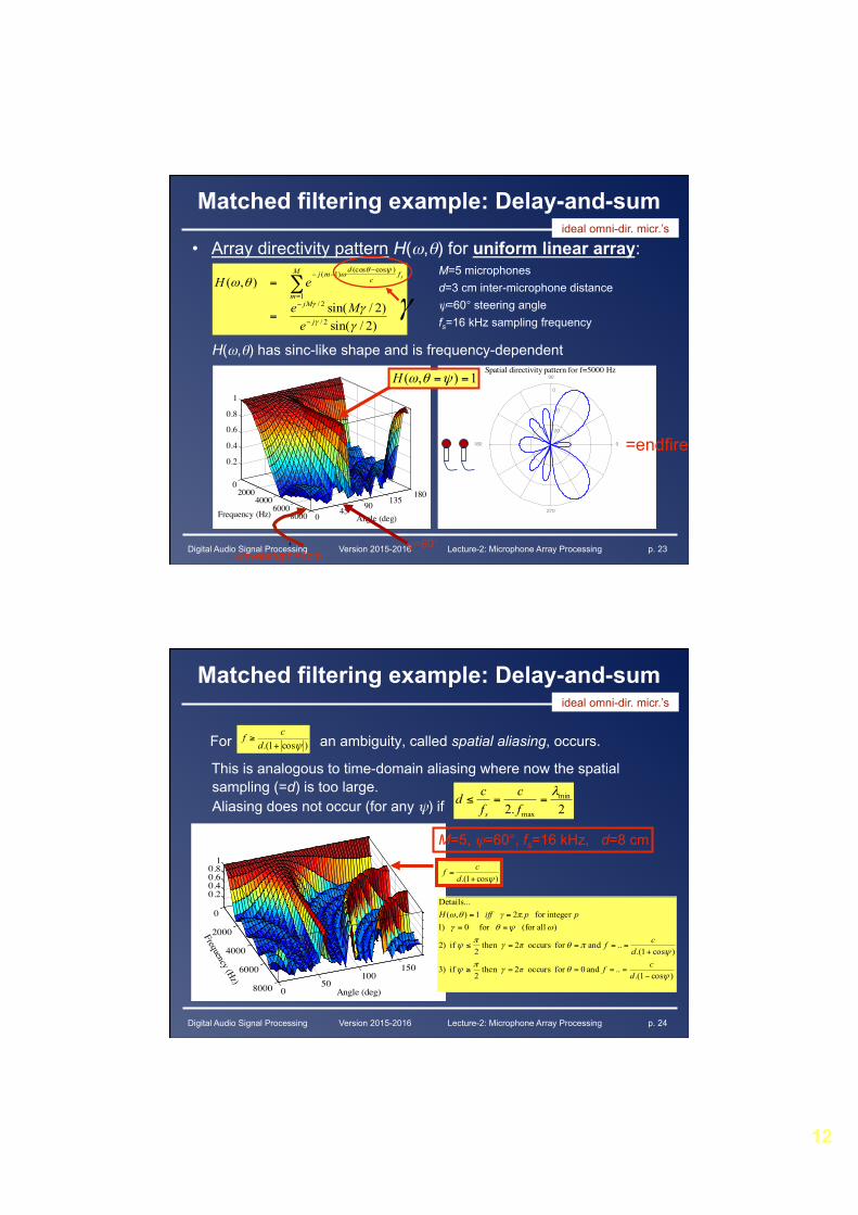
• Array directivity pattern H(ω,θ) for uniform linear array:
H(ω,θ) has sinc-like shape and is frequency-dependent
Matched filtering example: Delay-and-sum
)2/sin()2/sin(
),(
2/
2/1
)cos(cos)1(
γγ
θω
γ
γ
ψθω
j
jM
M
m
fc
dmj
eMe
eH s
−
−=
−−−
=
= ∑
-20
-10
0
90
270
180 0
Spatial directivity pattern for f=5000 Hz
M=5 microphones d=3 cm inter-microphone distance ψ=60° steering angle fs=16 kHz sampling frequency
=endfire
γ
1),( ==ψθωH
ψ=60° wavelength=4cm
ideal omni-dir. micr.’s
Digital Audio Signal Processing Version 2015-2016 Lecture-2: Microphone Array Processing p. 24
0
2000
4000
6000
8000 050
100150
0.20.40.60.8
1
Angle (deg)
Frequency (Hz)
Matched filtering example: Delay-and-sum
For an ambiguity, called spatial aliasing, occurs. This is analogous to time-domain aliasing where now the spatial
sampling (=d) is too large. Aliasing does not occur (for any ψ) if
M=5, ψ=60°, fs=16 kHz, d=8 cm
)cos1.(
ψ+=d
cf
2.2min
max
λ==≤
fc
fcds
)cos1.(
.. and 0for occurs 2 then2
if 3)
)cos1.(.. and for occurs 2 then
2 if 2)
) all(for for 0 )1integer for 2 1),(
Details...
ψθγ
πψ
ψπθγ
πψ
ωψθγ
θω
−====≥
+====≤
==
==
dcfπ
dcfπ
pπ.pγiffH
ideal omni-dir. micr.’s
)cos1.(
ψ+≥d
cf
13
Digital Audio Signal Processing Version 2015-2016 Lecture-2: Microphone Array Processing p. 25
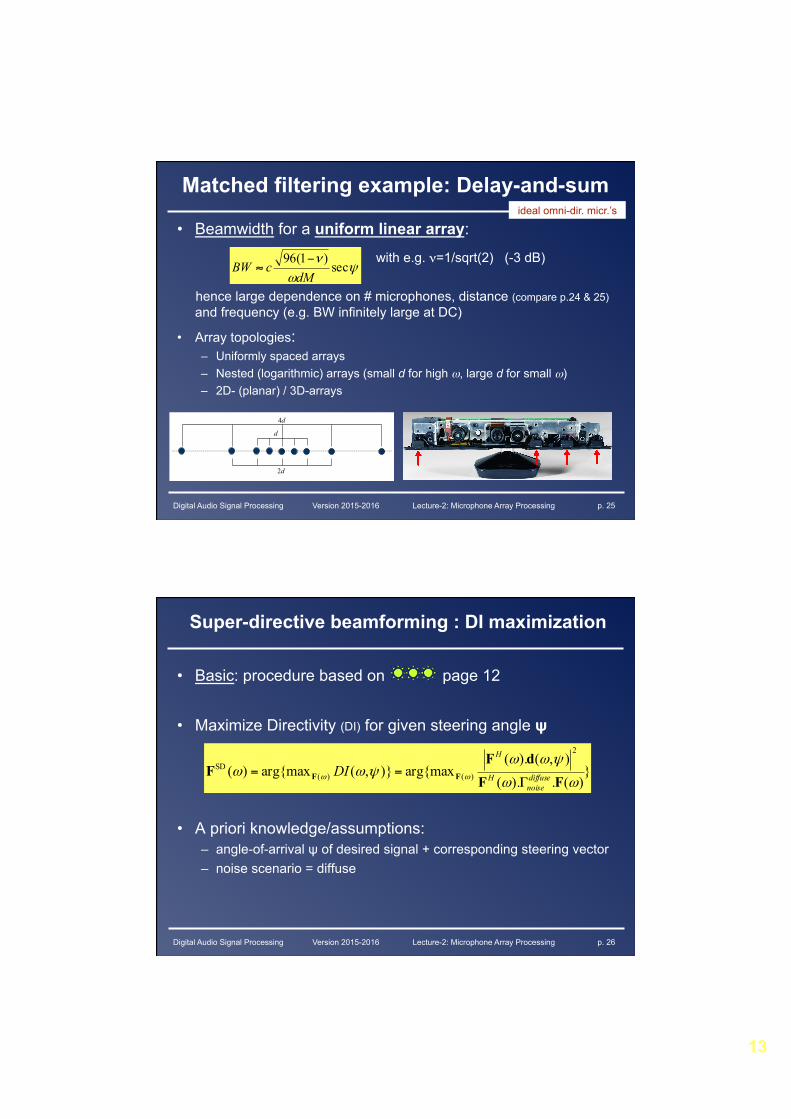
Matched filtering example: Delay-and-sum
• Beamwidth for a uniform linear array:
hence large dependence on # microphones, distance (compare p.24 & 25) and frequency (e.g. BW infinitely large at DC)
• Array topologies: – Uniformly spaced arrays – Nested (logarithmic) arrays (small d for high ω, large d for small ω) – 2D- (planar) / 3D-arrays
with e.g. ν=1/sqrt(2) (-3 dB)
d
2d
4d
ψω
νsec)1(96
dMcBW
−≈
ideal omni-dir. micr.’s
Digital Audio Signal Processing Version 2015-2016 Lecture-2: Microphone Array Processing p. 26
Super-directive beamforming : DI maximization
• Basic: procedure based on page 12
• Maximize Directivity (DI) for given steering angle ψ
• A priori knowledge/assumptions: – angle-of-arrival ψ of desired signal + corresponding steering vector – noise scenario = diffuse
})(.).(
),().(arg{max)},(arg{max)(
2
)()(SD
ωω
ψωωψωω ωω FF
dFF FF diffuse
noiseH
H
DIΓ
==

14
Digital Audio Signal Processing Version 2015-2016 Lecture-2: Microphone Array Processing p. 27
• Maximization in
is equivalent to minimization of noise output power (under diffuse input noise), subject to unit response for steering angle (**)
• Optimal solution is
• [FIR approximation]
})(.).(
),().(arg{max)(
2
)(SD
ωω
ψωωω ω FF
dFF F diffuse
noiseH
H
Γ=
1),().( s.t. ),().().(min )( =Γ ψωωωωωω dFFFFHdiffuse
noiseH
),(.)}(.{1)( 1
),(.1)}(.{),(
SD ψωωωψωωψω
dFdd
−−Γ
Γ= diffusenoisediffuse
noiseH
ωωωω
dNnMmf nm ∫ −−==
2SD1..0,..1, )()(min
,FF
Super-directive beamforming : DI maximization
Digital Audio Signal Processing Version 2015-2016 Lecture-2: Microphone Array Processing p. 28
• Directivity patterns for end-fire steering (ψ=0):
Superdirective beamformer has highest DI, but very poor WNG (at low frequencies, where diffuse noise coherence matrix becomes ill-conditioned) hence problems with robustness (e.g. sensor noise) !
-20
-10
0
90
270
180 0
Superdirective beamformer (f=3000 Hz)
-20
-10
0
90
270
180 0
Delay-and-sum beamformer (f=3000 Hz)
M=5 d=3 cm fs=16 kHz
Maximum directivity=M.M obtained for end-fire steering and for frequency->0 (no proof)
ideal omni-dir. micr.’s
0 2000 4000 6000 80000
5
10
15
20
25
Frequency (Hz)
Direc
tivity
(line
ar)
SuperdirectiveDelay-and-sum
0 2000 4000 6000 8000-60
-50
-40
-30
-20
-10
0
10
Frequency (Hz)
Whit
e nois
e gain
(dB)
SuperdirectiveDelay-and-sum
WNG=M= 5
PS: diffuse noise ≈ white noise for high frequencies (cfr. ωèΠ and c/fs=λmin/2≈min(dj-di) in diffuse noise coherence matrix)
DI=WNG=5
DI=M 2=25
Super-directive beamforming : DI maximization
15
Digital Audio Signal Processing Version 2015-2016 Lecture-2: Microphone Array Processing p. 29
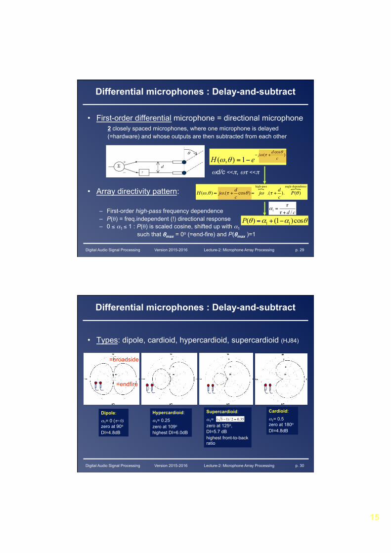
• First-order differential microphone = directional microphone 2 closely spaced microphones, where one microphone is delayed (=hardware) and whose outputs are then subtracted from each other
• Array directivity pattern:
– First-order high-pass frequency dependence – P(θ) = freq.independent (!) directional response – 0 ≤ α1 ≤ 1 : P(θ) is scaled cosine, shifted up with α1 such that θmax = 0o (=end-fire) and P(θmax )=1
d
Σ τ
θ
+
_
)cos(1),( c
djeH
θτω
θω+−
−=
ωd/c <<π, ωτ <<π
cd /1 +=τ
τα
θααθ cos)1()( 11 −+=P
H (ω,θ ) ≈ jω.(τ + dc
cosθ ) = jωhigh-pass!
.(τ + dc
). P(θ )angle dependence!
Differential microphones : Delay-and-subtract
Digital Audio Signal Processing Version 2015-2016 Lecture-2: Microphone Array Processing p. 30
Differential microphones : Delay-and-subtract
• Types: dipole, cardioid, hypercardioid, supercardioid (HJ84)
=endfire
=broadside
Dipole:
α1= 0 (τ=0) zero at 90o
DI=4.8dB
Cardioid:
α1= 0.5 zero at 180o
DI=4.8dB
Supercardioid:
α1= zero at 125o, DI=5.7 dB highest front-to-back ratio
35.02/)13( ≈−
Hypercardioid:
α1= 0.25 zero at 109o highest DI=6.0dB
16
Digital Audio Signal Processing Version 2015-2016 Lecture-2: Microphone Array Processing p. 31
Overview
• Introduction & beamforming basics – Data model & definitions
• Fixed beamforming – Filter-and-sum beamformer design – Matched filtering
• White noise gain maximization • Ex: Delay-and-sum beamforming
– Superdirective beamforming • Directivity maximization
– Directional microphones (delay-and-subtract)
• Adaptive Beamforming – LCMV beamformer – Generalized sidelobe canceler
Digital Audio Signal Processing Version 2015-2016 Lecture-2: Microphone Array Processing p. 32
LCMV beamformer
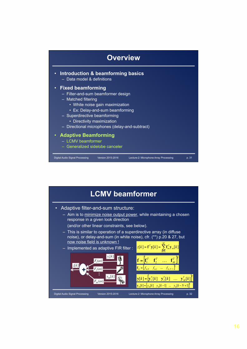
• Adaptive filter-and-sum structure: – Aim is to minimize noise output power, while maintaining a chosen
response in a given look direction (and/or other linear constraints, see below). – This is similar to operation of a superdirective array (in diffuse
noise), or delay-and-sum (in white noise), cfr. (**) p.20 & 27, but now noise field is unknown !
– Implemented as adaptive FIR filter :
[ ] ]1[...]1[][][ T+−−= Nkykykyk mmmmy
∑=
==M
mm
Tm
T kkkz1
][][][ yfyf
[ ]TTM
TT kkkk ][][][][ 21 yyyy …=
[ ]TTM
TT ffff …21=[ ] ... T
1,1,0, −= Nmmmm ffff
F1(ω)
F2 (ω)
FM (ω)
z[k]
y1[k]
+ : yM [k]
17
Digital Audio Signal Processing Version 2015-2016 Lecture-2: Microphone Array Processing p. 33
LCMV beamformer
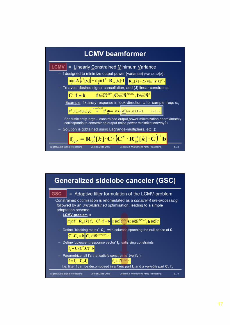
LCMV = Linearly Constrained Minimum Variance – f designed to minimize output power (variance) (read on..) z[k] :
– To avoid desired signal cancellation, add (J) linear constraints
Example: fix array response in look-direction ψ for sample freqs ωi
For sufficiently large J constrained output power minimization approximately corresponds to constrained output noise power minimization(why?)
– Solution is (obtained using Lagrange-multipliers, etc..):
Ryy[k]= E{y[k].y[k]T}{ } fRf
ff⋅⋅= ][min][min 2 kkzE yy
T
FT (ωi ).d(ωi,ψ) =Lecture2-p17
f T d(ωi,ψ) = dT (ωi,ψ).f =1 i =1..J
JJMNMNT ℜ∈ℜ∈ℜ∈= × bCfbfC ,, .
( ) bCRCCRf 111 ][][ −−− ⋅⋅⋅⋅= kk yyT
yyopt
Digital Audio Signal Processing Version 2015-2016 Lecture-2: Microphone Array Processing p. 34
Generalized sidelobe canceler (GSC)
GSC = Adaptive filter formulation of the LCMV-problem Constrained optimisation is reformulated as a constraint pre-processing,
followed by an unconstrained optimisation, leading to a simple adaptation scheme – LCMV-problem is
– Define `blocking matrix’ Ca, ,with columns spanning the null-space of C
– Define ‘quiescent response vector’ fq satisfying constraints
– Parametrize all f’s that satisfy constraints (verify!) I.e. filter f can be decomposed in a fixed part fq and a variable part Ca. fa
bfCfRff
=⋅⋅⋅ Tyy
T k ,][min
f = fq −Ca.fa
)( JMNMNa
−×ℜ∈C
JJMNMN ℜ∈ℜ∈ℜ∈ × bCf ,,
CT .Ca = 0
fq =C.(CT .C)−1b
fa ∈ℜ(MN−J )
18
Digital Audio Signal Processing Version 2015-2016 Lecture-2: Microphone Array Processing p. 35
Generalized sidelobe canceler
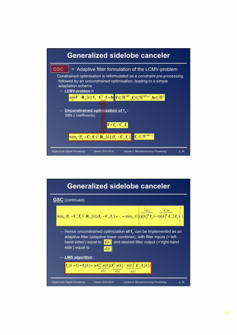
GSC = Adaptive filter formulation of the LCMV-problem Constrained optimisation is reformulated as a constraint pre-processing,
followed by an unconstrained optimisation, leading to a simple adaptation scheme – LCMV-problem is
– Unconstrained optimization of fa : (MN-J coefficients)
bfCfRff
=⋅⋅⋅ Tyy
T k ,][min JJMNMN ℜ∈ℜ∈ℜ∈ × bCf ,,
).].([.).(min aaqyyT
aaq ka
fCfRfCff −−
f = fq −Ca.fa
fa ∈ℜ(MN−J )
Digital Audio Signal Processing Version 2015-2016 Lecture-2: Microphone Array Processing p. 36
GSC (continued)
– Hence unconstrained optimization of fa can be implemented as an adaptive filter (adaptive linear combiner), with filter inputs (=‘left- hand sides’) equal to and desired filter output (=‘right-hand side’) equal to – LMS algorithm :
Generalized sidelobe canceler
}))..][().][({min...).].([.).(min
2][~][
aa
kd
qaaqyyT
aaq
T
aakkEk fCyfyfCfRfCf
ky
TTff
!"!#$!"!#$ΔΔ==
−==−−
][~ ky
][kd
])[..][][..(][..][]1[][~][][~
kkkkkk a
k
aT
kd
Tq
k
Taaa
T
fCyyfyCffyy!"!#$"#$!"!#$ −+=+ µ
19
Digital Audio Signal Processing Version 2015-2016 Lecture-2: Microphone Array Processing p. 37
Generalized sidelobe canceler
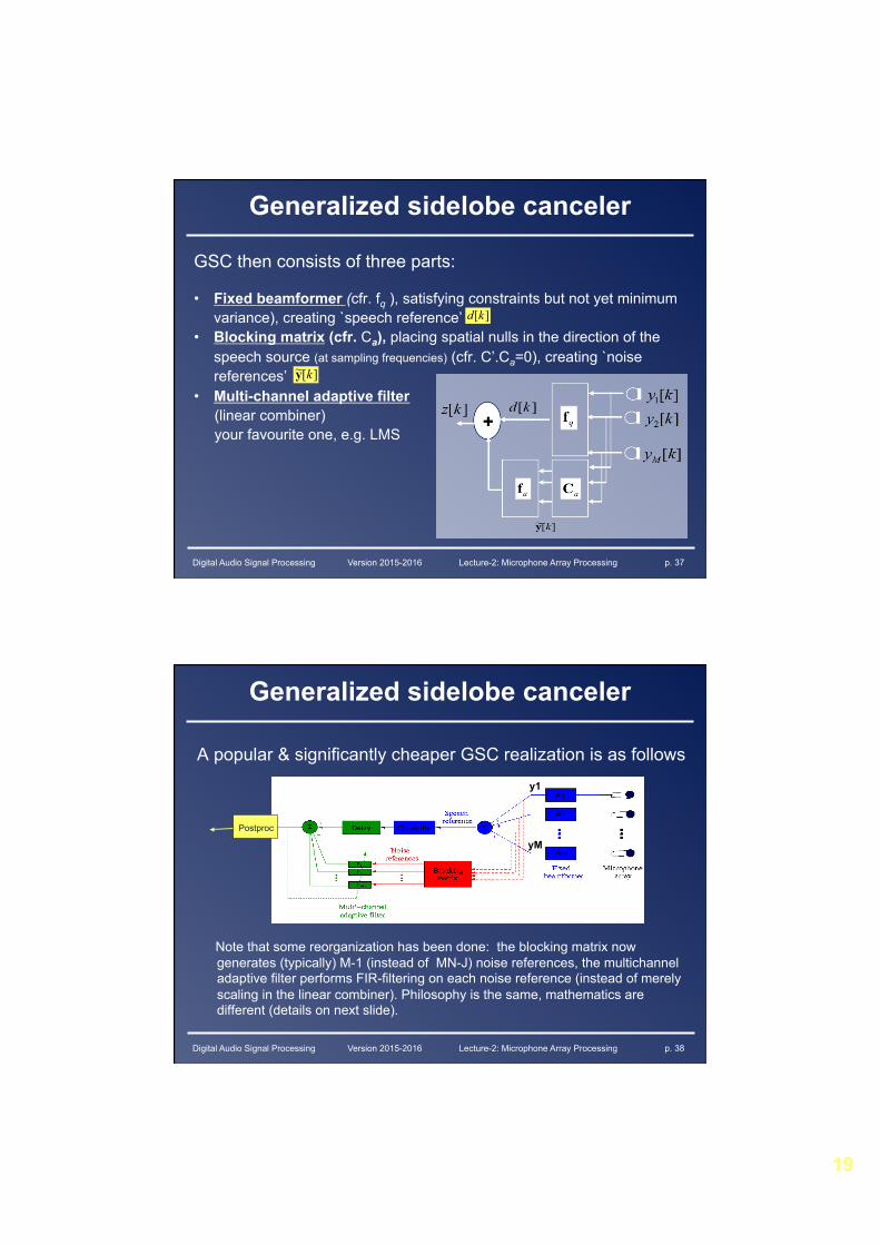
GSC then consists of three parts: • Fixed beamformer (cfr. fq ), satisfying constraints but not yet minimum
variance), creating `speech reference’ • Blocking matrix (cfr. Ca), placing spatial nulls in the direction of the
speech source (at sampling frequencies) (cfr. C’.Ca=0), creating `noise references’
• Multi-channel adaptive filter (linear combiner) your favourite one, e.g. LMS
][kd
][~ ky
Digital Audio Signal Processing Version 2015-2016 Lecture-2: Microphone Array Processing p. 38
Generalized sidelobe canceler
A popular & significantly cheaper GSC realization is as follows
Note that some reorganization has been done: the blocking matrix now generates (typically) M-1 (instead of MN-J) noise references, the multichannel adaptive filter performs FIR-filtering on each noise reference (instead of merely scaling in the linear combiner). Philosophy is the same, mathematics are different (details on next slide).
Postproc
y1
yM
20
Digital Audio Signal Processing Version 2015-2016 Lecture-2: Microphone Array Processing p. 39
Generalized sidelobe canceler
• Math details: (for Delta’s=0)
[ ][ ]
[ ]][.~][~
]1[~...]1[~][~][~
~...00:::0...~00...0~
][...][][][
]1[...]1[][][
][.][.][~
:1:1
:1:1:1
permuted,
21:1
:1:1:1permuted
permutedpermuted,
kk
Lkkkk
kykykyk
Lkkkk
kkk
MTaM
TTM
TM
TM
Ta
Ta
Ta
Ta
TMM
TTM
TM
TM
Ta
Ta
yCy
yyyy
C
CC
C
y
yyyy
yCyCy
=
+−−=
⎥⎥⎥⎥⎥
⎦
⎤
⎢⎢⎢⎢⎢
⎣
⎡
=
=
+−−=
==
=input to multi-channel adaptive filter
select `sparse’ blocking matrix such that :
=use this as blocking matrix now
Digital Audio Signal Processing Version 2015-2016 Lecture-2: Microphone Array Processing p. 40
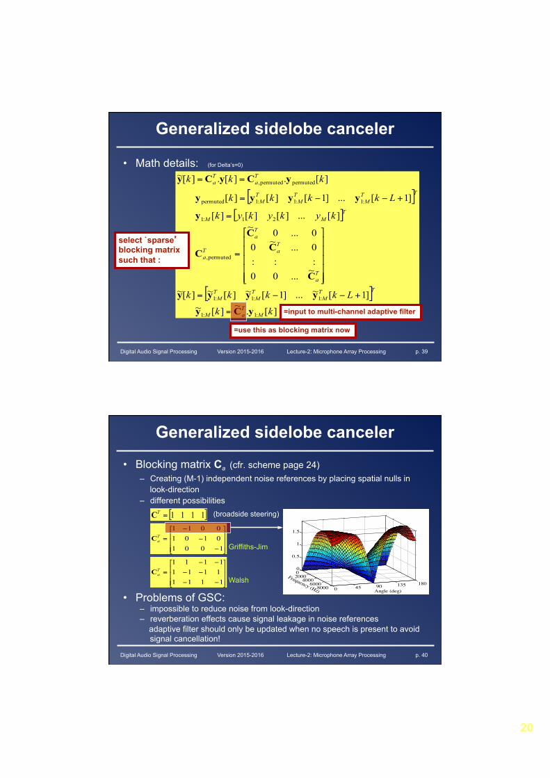
Generalized sidelobe canceler
• Blocking matrix Ca (cfr. scheme page 24) – Creating (M-1) independent noise references by placing spatial nulls in
look-direction – different possibilities
(broadside steering)
• Problems of GSC: – impossible to reduce noise from look-direction – reverberation effects cause signal leakage in noise references adaptive filter should only be updated when no speech is present to avoid
signal cancellation!
[ ]1111=TC
⎥⎥⎥
⎦
⎤
⎢⎢⎢
⎣
⎡
−
−
−
=
100101010011
TaC
⎥⎥⎥
⎦
⎤
⎢⎢⎢
⎣
⎡
−−
−−
−−
=
111111111111
TaC 0
20004000
60008000 0 45 90 135 180
0
0.5
1
1.5
Angle (deg)
Frequency (Hz)
Griffiths-Jim
Walsh