Embed Size (px)
Citation preview
Microphone Array Processing forRobust Speech Recognition
Michael L. Seltzer
Thesis Committee:Richard M. Stern, Chair
Tsuhan ChenGary W. Elko
B. V. K. Vijaya Kumar
Submitted to the Department of Electrical and Computer Engineering in partialfulfillment of the requirements for the degree of Doctor of Philosophy at
Carnegie Mellon UniversityPittsburgh, PA 15213
July 2003
Copyright c© 2003 Michael L. Seltzer


To my parents.

Abstract
Speech recognition performance degrades significantly in distant-talking environments, wherethe speech signals can be severely distorted by additive noise and reverberation. In suchenvironments, the use of microphone arrays has been proposed as a means of improvingthe quality of captured speech signals. Currently, microphone-array-based speech recogni-tion is performed in two independent stages: array processing and then recognition. Arrayprocessing algorithms designed for signal enhancement are applied in order to reduce thedistortion in the speech waveform prior to feature extraction and recognition.
This approach assumes that improving the quality of the speech waveform will neces-sarily result in improved recognition performance. However, speech recognition systems arestatistical pattern classifiers that process features derived from the speech waveform, not thewaveform itself. An array processing algorithm can therefore only be expected to improverecognition if it maximizes or at least increases the likelihood of the correct hypothesis,relative to other competing hypotheses.
In this thesis a new approach to microphone-array processing is proposed in which thegoal of the array processing is not to generate an enhanced output waveform but rather togenerate a sequence of features which maximizes the likelihood of the correct hypothesis.In this approach, called Likelihood Maximizing Beamforming (LIMABEAM), informationfrom the speech recognition system itself is used to optimize a filter-and-sum beamformer.Using LIMABEAM, significant improvements in recognition accuracy over conventionalarray processing approaches are obtained in moderately reverberant environments over awide range of signal-to-noise ratios. However, only limited improvements are obtained inenvironments with more severe reverberation.
To address this issue, a subband filtering approach to LIMABEAM is proposed, calledSubband-Likelihood Maximizing Beamforming (S-LIMABEAM). S-LIMABEAM employs anew subband filter-and-sum architecture which explicitly considers how the features used forrecognition are computed. This enables S-LIMABEAM to achieve dramatically improvedperformance over the original LIMABEAM algorithm in highly reverberant environments.
Because the algorithms in this thesis are data-driven, they do not require a priori knowl-edge of the room impulse response, nor any particular number of microphones or arraygeometry. To demonstrate this, LIMABEAM and S-LIMABEAM are evaluated using mul-tiple array configurations and environments including an array-equipped personal digitalassistant (PDA) and a meeting room with a few tabletop microphones. In all cases, theproposed algorithms significantly outperform conventional array processing approaches.
i

Acknowledgments
This thesis would not have been possible without the support and encouragement of manypeople. To the following people, I owe an enormous debt of gratitude.
My advisor, Professor Richard Stern, who welcomed me into his group when I arrivedat CMU knowing absolutely nothing about speech recognition. Rich gave me the guidanceI needed to become a capable researcher and the freedom to pursue my own ideas. He hasbeen a role model of professionalism and integrity, as well as a good friend.
Dr. Gary Elko, whose expertise in microphone arrays and acoustics was invaluable. Hewas very generous with his time and always quick to respond to my questions.
Professor B. V. K. Vijaya Kumar and Professor Tsuhan Chen, who made many valuablesuggestions that really improved the quality of this dissertation.
The members of the CMU Robust Speech Group, past and present, from whom I learneda great deal and with whom I shared many laughs. Rita Singh, Juan Huerta, and Sam-JooDoh never grew tired of answering my endless stream of questions during my first two yearshere. Jon Nedel, Evandro Gouvea, Xiang Li, and Pablo Hennings were always around fordiscussions and their camaraderie created a great work environment.
Bhiksha Raj, who has been a mentor, a collaborator, and a good friend. He taught menot to shy away from tough research problems and his positive attitude in the face of somedifficult circumstances amazes and inspires me.
Tom Sullivan and Yasunari Obuchi, who recorded the microphone array data used inthis thesis, and the ICSI speech group, who graciously gave me their meeting room data.
Kevin Dixon, Jay Wylie, Dan Gaugel, Stefanie Tomko, Mike Stout, George Lopez, andRich Malak, whose friendship was a constant reminder that there is more to graduate schoolthan research and work. They were a limitless source of support, fun, and laughs, and Ifeel extremely lucky to be able to call them my friends.
Julie, who has given me more love and encouragement during this process than anyonecan possibly ask for. Her boundless support kept me going when things were difficult, andI can’t wait to start the next chapter of my life with her.
My sister Gabrielle, who has been my biggest cheerleader throughout my life and towhom I have grown closer over the past five years, despite the distance between us.
Finally, there is no way I would be where I am today without the immeasurable love,support, and encouragement of my parents. I cannot thank them enough for all the oppor-tunities they have given me in my life and for always believing in me. They are an incredibleinspiration to me.
iii

Table of Contents
Abstract i
Acknowledgments iii
Table of Contents viii
List of Figures xi
List of Tables xiv
1 Introduction 1
1.1 What this thesis is about . . . . . . . . . . . . . . . . . . . . . . . . . . . . 3
1.2 Dissertation Outline . . . . . . . . . . . . . . . . . . . . . . . . . . . . . . . 4
2 A Review of Automatic Speech Recognition 7
2.1 Introduction . . . . . . . . . . . . . . . . . . . . . . . . . . . . . . . . . . . . 7
2.2 HMM-based Automatic Speech Recognition . . . . . . . . . . . . . . . . . . 7
2.2.1 Feature Extraction . . . . . . . . . . . . . . . . . . . . . . . . . . . . 8
2.2.2 HMM-based Modeling of Distributions of Feature Vectors . . . . . . 9
2.3 ASR Performance in Distant-talking Environments . . . . . . . . . . . . . . 14
2.3.1 The Effect of Additive Noise on Recognition Accuracy . . . . . . . . 14
2.3.2 The Effect of Reverberation on Recognition Accuracy . . . . . . . . 15
2.4 Summary . . . . . . . . . . . . . . . . . . . . . . . . . . . . . . . . . . . . . 20
3 Microphone Array Processing for Speech Recognition 21
3.1 Introduction . . . . . . . . . . . . . . . . . . . . . . . . . . . . . . . . . . . . 21
3.2 Fundamentals of Array Processing . . . . . . . . . . . . . . . . . . . . . . . 22
3.3 Microphone Array Processing Approaches . . . . . . . . . . . . . . . . . . . 26
3.3.1 Classical Beamforming . . . . . . . . . . . . . . . . . . . . . . . . . . 26
v

3.3.2 Adaptive Array Processing . . . . . . . . . . . . . . . . . . . . . . . 27
3.3.3 Additional Microphone Array Processing Methods . . . . . . . . . . 28
3.4 Speech Recognition Compensation Methods . . . . . . . . . . . . . . . . . . 31
3.4.1 CDCN and VTS . . . . . . . . . . . . . . . . . . . . . . . . . . . . . 31
3.4.2 Maximum Likelihood Linear Regression . . . . . . . . . . . . . . . . 32
3.5 Speech Recognition with Microphone Arrays . . . . . . . . . . . . . . . . . . 32
3.5.1 Experimental Setup and Corpora . . . . . . . . . . . . . . . . . . . . 33
3.5.2 Evaluating Performance and Determining Statistical Significance . . 34
3.5.3 Recognition Results . . . . . . . . . . . . . . . . . . . . . . . . . . . 35
3.6 Summary . . . . . . . . . . . . . . . . . . . . . . . . . . . . . . . . . . . . . 37
4 Likelihood Maximizing Beamforming 39
4.1 Introduction . . . . . . . . . . . . . . . . . . . . . . . . . . . . . . . . . . . . 39
4.2 Filter-and-Sum Array Processing . . . . . . . . . . . . . . . . . . . . . . . . 40
4.3 Likelihood Maximizing Beamforming (LIMABEAM) . . . . . . . . . . . . . 41
4.4 Optimizing the State Sequence . . . . . . . . . . . . . . . . . . . . . . . . . 43
4.5 Optimizing the Array Parameters . . . . . . . . . . . . . . . . . . . . . . . . 43
4.5.1 Gaussian State Output Distributions . . . . . . . . . . . . . . . . . . 44
4.5.2 Mixture of Gaussians State Output Distributions . . . . . . . . . . . 45
4.5.3 Gradient-based Array Parameter Optimization . . . . . . . . . . . . 46
4.6 Evaluating LIMABEAM Using Oracle State Sequences . . . . . . . . . . . . 46
4.6.1 Experiments Using Gaussian Distributions . . . . . . . . . . . . . . . 47
4.6.2 Experiments Using Mixtures of Gaussians . . . . . . . . . . . . . . . 50
4.6.3 Summary of Results Using Oracle LIMABEAM . . . . . . . . . . . . 51
4.7 The Calibrated LIMABEAM Algorithm . . . . . . . . . . . . . . . . . . . . 51
4.7.1 Experimental Results Using Calibrated LIMABEAM . . . . . . . . . 54
4.7.2 Summary of Results Using Calibrated LIMABEAM . . . . . . . . . 56
4.8 The Unsupervised LIMABEAM Algorithm . . . . . . . . . . . . . . . . . . 57
4.8.1 Experimental Results Using Unsupervised LIMABEAM . . . . . . . 58
4.8.2 Summary of Results Using Unsupervised LIMABEAM . . . . . . . . 61
4.9 Analysis of Optimized Array Parameters and the Output Waveform . . . . 61
4.9.1 The Optimized Filters of the Array . . . . . . . . . . . . . . . . . . . 62
4.9.2 The Array Output Waveform . . . . . . . . . . . . . . . . . . . . . . 65
4.10 Other Considerations . . . . . . . . . . . . . . . . . . . . . . . . . . . . . . . 65
4.10.1 Incorporating Feature Mean Normalization . . . . . . . . . . . . . . 65
4.10.2 Sum-and-Filter Processing . . . . . . . . . . . . . . . . . . . . . . . . 67
4.10.3 Combining LIMABEAM with Other Compensation Techniques . . . 68
4.10.4 Computational Complexity . . . . . . . . . . . . . . . . . . . . . . . 69
4.11 Summary . . . . . . . . . . . . . . . . . . . . . . . . . . . . . . . . . . . . . 70
5 Subband-Likelihood Maximizing Beamforming 73
5.1 Introduction . . . . . . . . . . . . . . . . . . . . . . . . . . . . . . . . . . . . 73
5.2 LIMABEAM in Highly Reverberant Environments . . . . . . . . . . . . . . 74
5.3 An Overview of Subband Adaptive Filtering . . . . . . . . . . . . . . . . . . 76
5.4 Subband Filtering for Microphone-array-based Speech Recognition . . . . . 78
5.4.1 Incorporating Subband Processing into the ASR Front-End . . . . . 78
5.4.2 Subband Filter-and-Sum Array Processing . . . . . . . . . . . . . . . 79
5.5 Subband-Likelihood Maximizing Beamforming (S-LIMABEAM) . . . . . . . 80
5.5.1 Feature-based Subband Filtering . . . . . . . . . . . . . . . . . . . . 81
5.5.2 Maximum Likelihood Estimation of Subband Filter Parameters . . . 81
5.6 Optimizing the Subband Filter Parameters . . . . . . . . . . . . . . . . . . 82
5.6.1 Gaussian State Output Distributions . . . . . . . . . . . . . . . . . . 84
5.6.2 Mixture of Gaussians State Output Distributions . . . . . . . . . . . 84
5.7 Analysis of the Dimensionality of Subband Filtering . . . . . . . . . . . . . 85
5.8 Applying S-LIMABEAM to Reverberant Speech . . . . . . . . . . . . . . . 86
5.9 Evaluating S-LIMABEAM Using Oracle State Sequences . . . . . . . . . . . 87
5.10 The Calibrated S-LIMABEAM Algorithm . . . . . . . . . . . . . . . . . . . 89
5.10.1 Experimental Results Using Calibrated S-LIMABEAM . . . . . . . . 90
5.11 The Unsupervised S-LIMABEAM Algorithm . . . . . . . . . . . . . . . . . 94
5.11.1 Experimental Results Using Unsupervised S-LIMABEAM . . . . . . 94
5.12 Computational Complexity . . . . . . . . . . . . . . . . . . . . . . . . . . . 97
5.13 Dimensionality Reduction via Parameter Sharing . . . . . . . . . . . . . . . 98
5.13.1 Sharing Parameters Within Mel Spectral Components . . . . . . . . 99
5.13.2 Sharing Parameters Across Mel Spectral Components . . . . . . . . 99
5.13.3 Experimental Results Using Parameter Sharing . . . . . . . . . . . . 100
5.14 S-LIMABEAM in Environments with Low Reverberation . . . . . . . . . . 100
5.15 Summary . . . . . . . . . . . . . . . . . . . . . . . . . . . . . . . . . . . . . 102
6 LIMABEAM in Other Multi-Microphone Environments 105
6.1 Introduction . . . . . . . . . . . . . . . . . . . . . . . . . . . . . . . . . . . . 105
6.2 Multi-microphone Speech Recognition on a PDA . . . . . . . . . . . . . . . 106
6.3 The CMU WSJ PDA corpus . . . . . . . . . . . . . . . . . . . . . . . . . . 107
6.3.1 Experimental Results Using LIMABEAM . . . . . . . . . . . . . . . 108
6.3.2 Summary of Experimental Results . . . . . . . . . . . . . . . . . . . 112
6.4 Meeting Transcription with Multiple Tabletop Microphones . . . . . . . . . 112
6.5 The ICSI Meeting Recorder Corpus . . . . . . . . . . . . . . . . . . . . . . . 113
6.5.1 Experimental Results Using S-LIMABEAM . . . . . . . . . . . . . . 114
6.6 Summary . . . . . . . . . . . . . . . . . . . . . . . . . . . . . . . . . . . . . 115
7 Summary and Conclusions 117
7.1 Introduction . . . . . . . . . . . . . . . . . . . . . . . . . . . . . . . . . . . . 117
7.2 Summary of Findings and Contributions of This Thesis . . . . . . . . . . . 118
7.3 Some Remaining Questions . . . . . . . . . . . . . . . . . . . . . . . . . . . 120
7.4 Directions for Further Research . . . . . . . . . . . . . . . . . . . . . . . . . 121
A Derivation of the Jacobian Matrix for LIMABEAM 125
A.1 Introduction . . . . . . . . . . . . . . . . . . . . . . . . . . . . . . . . . . . . 125
A.2 Computing Mel Frequency Cepstral Coefficients . . . . . . . . . . . . . . . . 126
A.3 Computing the Elements of the Jacobian Matrix . . . . . . . . . . . . . . . 127
B Parameter Reduction using ASR-based Subband Filtering 131
C Derivation of the Gradient Vector for S-LIMABEAM 135
C.1 Introduction . . . . . . . . . . . . . . . . . . . . . . . . . . . . . . . . . . . . 135
C.2 Defining the Gradient Vector . . . . . . . . . . . . . . . . . . . . . . . . . . 135
C.3 Computing the Elements of the Gradient Vector . . . . . . . . . . . . . . . 136
C.4 Sharing Filter Parameters Within Mel Spectral Components . . . . . . . . . 138
C.5 Sharing Filter Parameters Across Mel Spectral Components . . . . . . . . . 139
References 141

List of Figures
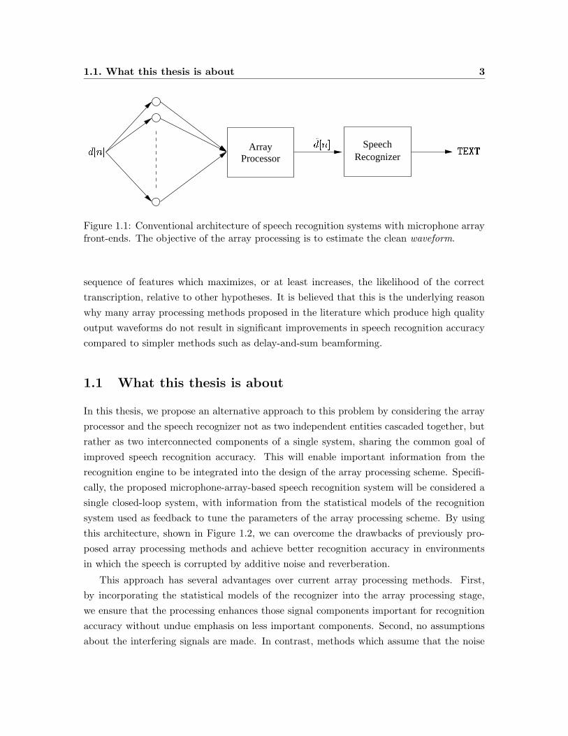
1.1 Conventional architecture of speech recognition systems with microphone
array front-ends. . . . . . . . . . . . . . . . . . . . . . . . . . . . . . . . . . 3
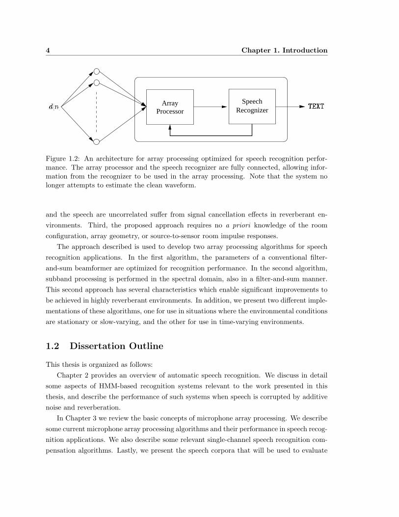
1.2 An architecture for array processing optimized for speech recognition perfor-
mance. . . . . . . . . . . . . . . . . . . . . . . . . . . . . . . . . . . . . . . . 4
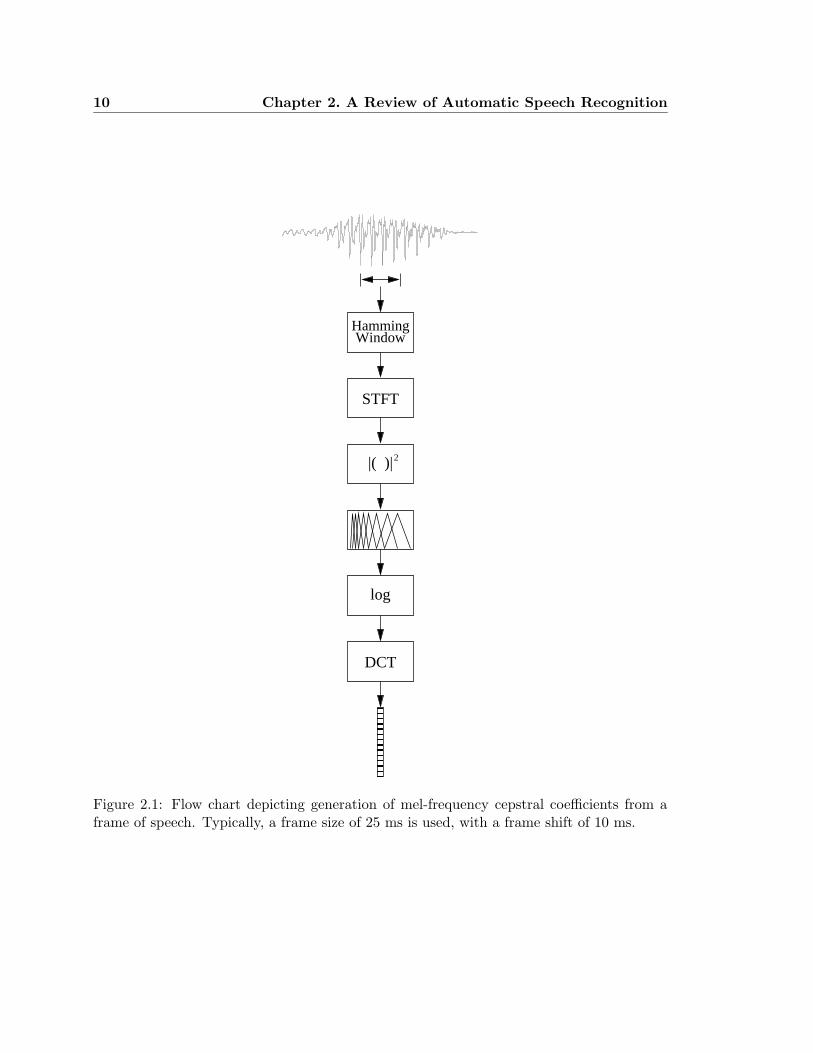
2.1 Flow chart depicting generation of mel-frequency cepstral coefficients from a
frame of speech. . . . . . . . . . . . . . . . . . . . . . . . . . . . . . . . . . . 10
2.2 An example of a 5-state left-to-right HMM. . . . . . . . . . . . . . . . . . . 11
2.3 An HMM for a sequence of words can be built from the individual HMMs of
its constituent words. . . . . . . . . . . . . . . . . . . . . . . . . . . . . . . . 13
2.4 WER vs. SNR for speech corrupted by additive white noise when the recog-
nition system is trained on clean speech. . . . . . . . . . . . . . . . . . . . . 15
2.5 WER vs. distance from the user to the microphone in an anechoic room.
A fixed white noise source was placed 1 m from the microphone, while the
user’s distance to the microphone was varied. . . . . . . . . . . . . . . . . . 15
2.6 The room impulse response from a room with a reverberation time of 0.47 s
measured using the TSP method. . . . . . . . . . . . . . . . . . . . . . . . . 17
2.7 Wideband spectrograms of the utterance “AND EXPECTS THE NUMBER” for (a)
close-talking recording (b) T60 = 0.2 s (c) T60 = 0.5 s (d) T60 = 0.75 s. . . . 18
2.8 WER vs. reverberation time when the recognition system is trained on clean
speech recorded from a close-talking microphone. . . . . . . . . . . . . . . . 19
2.9 WER vs. distance from the user to the microphone in an room with a
reverberation time of 0.2 s. . . . . . . . . . . . . . . . . . . . . . . . . . . . 19
3.1 (a) Two acoustic sources propagating toward two microphones. (b) The
additional distance the source travels to m1 can be determined based on the
angle of arrival θ and the distance between the microphones d. . . . . . . . 23
ix
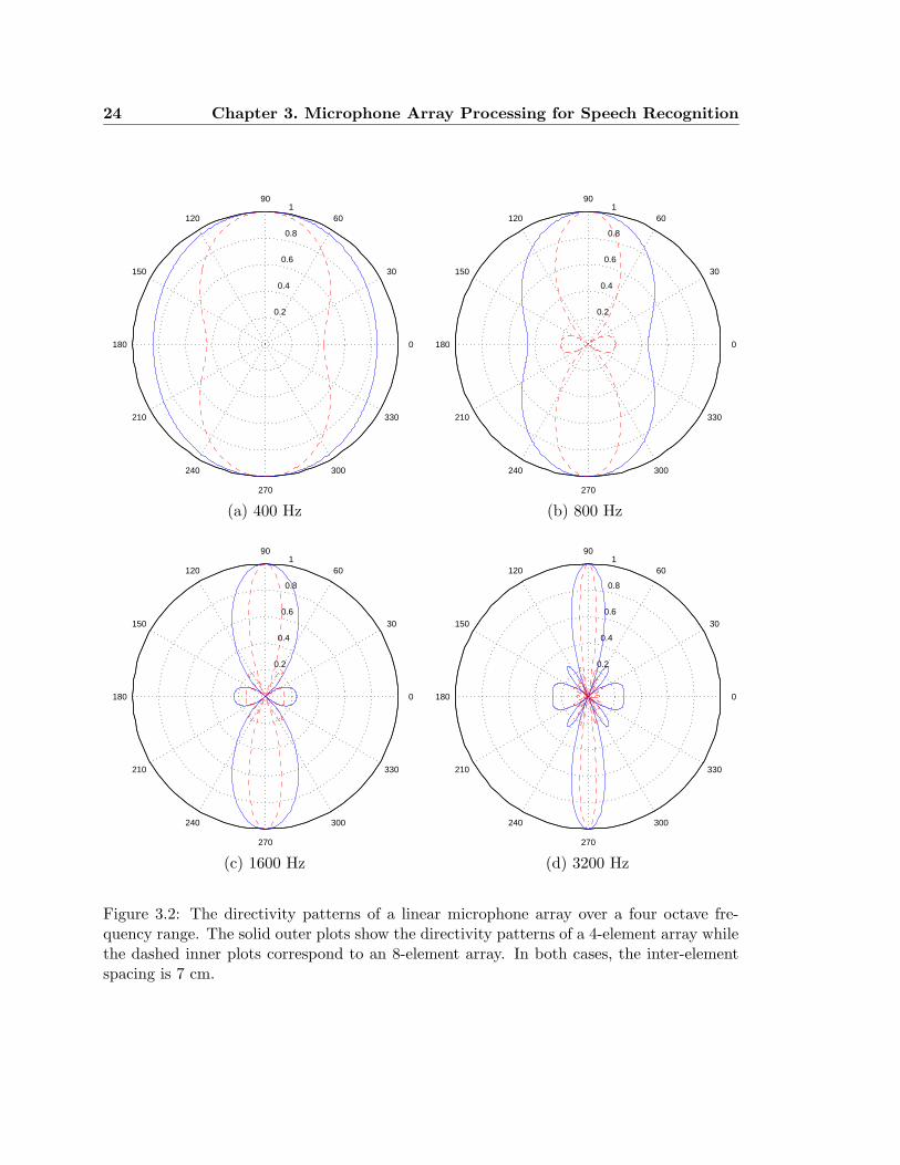
3.2 The directivity patterns of a linear microphone array over a four octave
frequency range. . . . . . . . . . . . . . . . . . . . . . . . . . . . . . . . . . 24
3.3 The beampatterns for the same microphone array configurations used in Fig-
ure 3.2 at frequencies which violate the spatial sampling theorem. The large
unwanted sidelobes are the result of spatial aliasing. . . . . . . . . . . . . . 25
3.4 The Griffiths-Jim Generalized Sidelobe Canceller . . . . . . . . . . . . . . . 28
3.5 Speech recognition performance on the CMU-8 corpus using a single channel,
delay-and-sum beamforming, and the GSC adapting only during silence regions. 36
3.6 WER obtained on the reverberant WSJ corpora using a single microphone
and delay-and-sum beamforming, shown as a function of reverberation time. 37
4.1 WER vs. filter length for the proposed array processing approach. The filter
parameters were optimized using a state sequence derived from the close-
talking signal and the transcript. . . . . . . . . . . . . . . . . . . . . . . . . 49
4.2 WER vs. the number of iterations of filter optimization for the proposed
array processing approach. The filter parameters were optimized using a
state sequence derived from the close-talking signal and the transcript. The
circles show the average number of iterations to convergence in each case. . 49
4.3 The WER obtained using oracle state sequences in the LIMABEAM algorithm. 50
4.4 Flowchart of LIMABEAM Calibration . . . . . . . . . . . . . . . . . . . . . 53
4.5 WER vs. filter length obtained using the Calibrated LIMABEAM algorithm. 55
4.6 Flowchart of Unsupervised LIMABEAM . . . . . . . . . . . . . . . . . . . . 59
4.7 WER vs. the average utterance duration obtained using the Unsupervised
LIMABEAM approach. . . . . . . . . . . . . . . . . . . . . . . . . . . . . . 60
4.8 Overall look-direction frequency response of the filter-and-sum beamformer
obtained by performing Calibrated LIMABEAM on an utterance from the
CMU-8 corpus. . . . . . . . . . . . . . . . . . . . . . . . . . . . . . . . . . . 63
4.9 Beampatterns of the filter-and-sum beamformer obtained by performing Cal-
ibrated LIMABEAM on an utterance from the CMU-8 corpus. . . . . . . . 64
4.10 Spectrograms of an utterance from the CMU-8 corpus obtained using (a) sin-
gle microphone only, (b) delay-and-sum beamforming (c) Calibrated LIMABEAM,
and (d) the close-talking microphone. . . . . . . . . . . . . . . . . . . . . . 66
4.11 Frequency response of the post-filter optimized using unsupervised maximum
likelihood filter optimization applied to the delay-and-sum output signal. . . 68
4.12 WER obtained by performing unsupervised maximum likelihood filter op-
timization on a post-filter applied to the output of a delay-and-sum beam-
former, shown as a function of the length of the post-filter. . . . . . . . . . 69
4.13 Average times-real-time to convergence of the LIMABEAM algorithm to op-
timize 20-tap filters for a single microphone and for an array of 8 microphones. 71
5.1 WER as a function of filter length for the WSJ0.47 corpus when the filter
parameters are optimized using Calibrated LIMABEAM. . . . . . . . . . . 75
5.2 A block diagram of conventional subband adaptive filtering. . . . . . . . . . 77
5.3 S-LIMABEAM for an array of two microphones for the lth log mel spectral
component which is composed of three subbands. . . . . . . . . . . . . . . . 83
5.4 The maximum number of parameters per microphone that need to be jointly
optimized as a function of the effective filter length in frames. . . . . . . . . 87
5.5 WER obtained using Oracle S-LIMABEAM for the WSJ0.47 corpus. . . . . 88
5.6 WER obtained using Calibrated S-LIMABEAM vs. the number of taps used
in each subband filter for single speaker from the WSJ0.47 corpus. . . . . . . 91
5.7 Log mel spectrograms of a segment of an utterance from the WSJ0.47 corpus
obtained from (a) a single channel in the array, (b) delay-and-sum beam-
forming, (c) the Calibrated S-LIMABEAM algorithm with 5 taps per filter,
and (d) the close-talking microphone signal. . . . . . . . . . . . . . . . . . . 92
5.8 WER obtained using Calibrated S-LIMABEAM shown as a function of re-
verberation time for the reverberant WSJ corpora. . . . . . . . . . . . . . . 93
5.9 WER obtained using Unsupervised S-LIMABEAM vs. the number of taps
used in each subband filter for the WSJ0.47 corpus. . . . . . . . . . . . . . . 95
5.10 WER obtained using Unsupervised S-LIMABEAM on the WSJ0.47 corpus as
a function of the number of iterations of optimization performed. . . . . . . 97
5.11 Average times-real-time to convergence of the subband filter parameter opti-
mization for one log mel spectral component using subband filters with 1 tap
and 5 taps and single Gaussians or mixtures of 8 Gaussians in the likelihood
expression. . . . . . . . . . . . . . . . . . . . . . . . . . . . . . . . . . . . . 98
6.1 A 4-microphone PDA mockup used to record the CMU WSJ PDA corpus . 107
6.2 WER obtained using the Calibrated LIMABEAM method on (a) the PDA-A
corpus and (b) the PDA-B corpus . . . . . . . . . . . . . . . . . . . . . . . 109
6.3 WER obtained using the Unsupervised LIMABEAM on (a) the PDA-A cor-
pus and (b) the PDA-B corpus . . . . . . . . . . . . . . . . . . . . . . . . . 111
6.4 The recording environment used in the ICSI Meeting Recorder corpus. . . . 114
6.5 WER obtained on the connected digits portion of the ICSI meeting data,
using only the PZM tabletop microphones. . . . . . . . . . . . . . . . . . . . 116

List of Tables
4.1 WER obtained using Calibrated LIMABEAM on the CMU-8 corpus for dif-
ferent calibration utterance durations. . . . . . . . . . . . . . . . . . . . . . 56
4.2 WER obtained using multiple iterations of LIMABEAM calibration on the
CMU-8 corpus. . . . . . . . . . . . . . . . . . . . . . . . . . . . . . . . . . . 56
4.3 WER obtained using Unsupervised LIMABEAM on the CMU-8 corpus. . . 58
4.4 WER obtained using multiple iterations of Unsupervised LIMABEAM on
the CMU-8 corpus. . . . . . . . . . . . . . . . . . . . . . . . . . . . . . . . . 61
4.5 WER obtained when delay-and-sum beamforming and Calibrated LIMABEAM
are followed by CDCN on the CMU-8 corpus. . . . . . . . . . . . . . . . . . 70
4.6 WER obtained when delay-and-sum beamforming and Unsupervised LIMABEAM
are followed by CDCN on the CMU-8 corpus. . . . . . . . . . . . . . . . . . 70
5.1 WER obtained using the Calibrated LIMABEAM algorithm for the WSJ0.47
corpus when 100-tap FIR filters are optimized using different amounts of
calibration data. . . . . . . . . . . . . . . . . . . . . . . . . . . . . . . . . . 75
5.2 WER obtained using Unsupervised S-LIMABEAM on the WSJ0.3 corpus . 96
5.3 Performance obtained using S-LIMABEAM using different methods of shar-
ing subband filter parameters. . . . . . . . . . . . . . . . . . . . . . . . . . . 101
5.4 WER obtained on the CMU-8 corpus using unsupervised array parameter op-
timization for the fullband filter-and-sum architecture described in Chapter
4 and the three subband architectures described in this chapter. . . . . . . . 102
6.1 WER obtained for the two WSJ PDA test sets using a 1 far-field microphone,
delay-and-sum beamforming with 2 or 4 microphones or the close-talking
reference microphone . . . . . . . . . . . . . . . . . . . . . . . . . . . . . . . 108
6.2 WER obtained using Unsupervised LIMABEAM when the state sequences
for optimization are derived using hypotheses obtained from delay-and-sum
beamforming or from Calibrated LIMABEAM . . . . . . . . . . . . . . . . . 111
xiii

Chapter 1
Introduction
State-of-the-art automatic speech recognition (ASR) systems are known to perform reason-
ably well when the speech signals are captured in a noise-free environment using a close-
talking microphone worn near the mouth of the speaker. Such technology has progressed
to the point where commercial systems have been deployed for some small tasks. However,
the benefits of speech-driven interfaces have yet to be fully realized, due in large part to the
significant degradation in performance these systems exhibit in real-world environments.
In such environments, the signal may be corrupted by a wide variety of sources including
additive noise, linear and non-linear distortion, transmission and coding effects, and other
phenomena.
This thesis is particularly interested in those environments in which either safety or
convenience preclude the use of a close-talking microphone. For example, while operating
a vehicle, the very act of wearing a microphone is distracting and dangerous. In a meeting
room, microphones restrict the movement of the participants by tethering them to their
seats by wires. And it is unlikely that users of an information kiosk will want to put on
a headset before asking for help. In all of these situations, wires can break and tangle,
creating a frustrating experience for the user.
In such settings, a better alternative to head-mounted microphones is to place a fixed
microphone some distance from the user. Unfortunately, as the distance between the user
and the microphone grows, the speech signal becomes increasingly degraded by the effects
of additive noise and reverberation, which in turn degrade speech recognition accuracy. In
such distant-talking environments, the use of an array of microphones, rather than a single
microphone, can compensate for this distortion by providing spatial filtering to the sound
field, effectively focusing attention in a desired direction.
Many signal processing techniques using arrays of sensors have been proposed in speech
1
2 Chapter 1. Introduction
and other application domains which improve the quality of the output signal and achieve
a substantial improvement in the signal-to-noise ratio (SNR). The most well-known general
class of array processing methods are beamforming methods. Beamforming refers to any
method that algorithmically, rather than physically, steers the sensors in the array toward a
target signal. The direction the array is steered is commonly called the look direction. The
simplest and most common method of beamforming is called delay-and-sum (Johnson &
Dudgeon, 1993). In delay-and-sum beamforming, the signals received by the microphones in
the array are time-aligned with respect to each other in order to adjust for the path-length
differences between the speech source and each of the microphones. The now time-aligned
signals are then weighted and added together. Any interfering signals from noise sources
that are not coincident with the speech source remain misaligned and are thus attenuated
when the signals are combined. A natural extension to delay-and-sum beamforming is filter-
and-sum beamforming, in which each microphone has an associated filter, and the received
signals are first filtered and then combined.
If the weights or filter parameters are adjusted online during processing, the methods
are referred to as adaptive beamforming techniques. These methods, such as (Frost, 1972;
Griffiths & Jim, 1982), update the array parameters on a sample-by-sample or frame-by-
frame basis according to a specified criterion. Typical criteria used in adaptive beamforming
include a distortionless response in the look direction and/or the minimization of the energy
from all directions not considered the look direction.
Conventionally, speech recognition using microphone arrays is generally performed in
two independent stages: array processing and then recognition. The array processing is
considered a pre-processing step to enhance the waveform prior to conventional feature
extraction and recognition. In this approach, the array processing is used to produce an
enhanced output waveform, as measured quantitatively by SNR or other distortion metric,
or by improved scores on perceptual tests by human listeners. A sequence of speech recogni-
tion feature vectors are derived from this enhanced waveform and passed to the recognition
engine for decoding. This configuration is depicted in Figure 1.1.
This approach to microphone array processing for speech recognition suffers from several
drawbacks. Most notably, it implicitly makes the assumption that generating a higher qual-
ity output waveform will necessarily result in improved recognition performance. However,
a speech recognition system does not interpret waveform-level information directly. It is a
statistical pattern classifier whose goal is to hypothesize the correct transcription. This is
usually accomplished by finding the word string that has the maximum likelihood of gen-
erating the sequence of features derived from the observed waveform. As a result, an array
processing scheme can only be expected to improve recognition accuracy if it generates a
1.1. What this thesis is about 3
RecognizerSpeechArray
Processor���������� � �
��� �
Figure 1.1: Conventional architecture of speech recognition systems with microphone arrayfront-ends. The objective of the array processing is to estimate the clean waveform.
sequence of features which maximizes, or at least increases, the likelihood of the correct
transcription, relative to other hypotheses. It is believed that this is the underlying reason
why many array processing methods proposed in the literature which produce high quality
output waveforms do not result in significant improvements in speech recognition accuracy
compared to simpler methods such as delay-and-sum beamforming.
1.1 What this thesis is about
In this thesis, we propose an alternative approach to this problem by considering the array
processor and the speech recognizer not as two independent entities cascaded together, but
rather as two interconnected components of a single system, sharing the common goal of
improved speech recognition accuracy. This will enable important information from the
recognition engine to be integrated into the design of the array processing scheme. Specifi-
cally, the proposed microphone-array-based speech recognition system will be considered a
single closed-loop system, with information from the statistical models of the recognition
system used as feedback to tune the parameters of the array processing scheme. By using
this architecture, shown in Figure 1.2, we can overcome the drawbacks of previously pro-
posed array processing methods and achieve better recognition accuracy in environments
in which the speech is corrupted by additive noise and reverberation.
This approach has several advantages over current array processing methods. First,
by incorporating the statistical models of the recognizer into the array processing stage,
we ensure that the processing enhances those signal components important for recognition
accuracy without undue emphasis on less important components. Second, no assumptions
about the interfering signals are made. In contrast, methods which assume that the noise
4 Chapter 1. Introduction
ArrayProcessor Recognizer
Speech ���������� �
Figure 1.2: An architecture for array processing optimized for speech recognition perfor-mance. The array processor and the speech recognizer are fully connected, allowing infor-mation from the recognizer to be used in the array processing. Note that the system nolonger attempts to estimate the clean waveform.
and the speech are uncorrelated suffer from signal cancellation effects in reverberant en-
vironments. Third, the proposed approach requires no a priori knowledge of the room
configuration, array geometry, or source-to-sensor room impulse responses.
The approach described is used to develop two array processing algorithms for speech
recognition applications. In the first algorithm, the parameters of a conventional filter-
and-sum beamformer are optimized for recognition performance. In the second algorithm,
subband processing is performed in the spectral domain, also in a filter-and-sum manner.
This second approach has several characteristics which enable significant improvements to
be achieved in highly reverberant environments. In addition, we present two different imple-
mentations of these algorithms, one for use in situations where the environmental conditions
are stationary or slow-varying, and the other for use in time-varying environments.
1.2 Dissertation Outline
This thesis is organized as follows:
Chapter 2 provides an overview of automatic speech recognition. We discuss in detail
some aspects of HMM-based recognition systems relevant to the work presented in this
thesis, and describe the performance of such systems when speech is corrupted by additive
noise and reverberation.
In Chapter 3 we review the basic concepts of microphone array processing. We describe
some current microphone array processing algorithms and their performance in speech recog-
nition applications. We also describe some relevant single-channel speech recognition com-
pensation algorithms. Lastly, we present the speech corpora that will be used to evaluate
1.2. Dissertation Outline 5
the techniques proposed in this thesis.
In Chapter 4 we introduce the framework used to develop the algorithms in this thesis.
We show how the objectives of the array processor and the speech recognizer can be unified,
and then develop and evaluate a filter-and-sum beamforming algorithm that does so.
In Chapter 5 we look more closely at the difficulties of recognizing speech in highly
reverberant environments. We present an algorithm which incorporates subband filtering
into the framework established in Chapter 4 and show that this approach is able to overcome
many of the difficulties encountered by previous dereverberation methods.
In Chapter 6 we apply the proposed algorithms to two alternative multi-channel speech
recognition applications. We show that the methods presented are capable of good perfor-
mance even in highly sub-optimal microphone configurations.
Finally, Chapter 7 summarizes the major results and contributions of this thesis and
highlights some directions for further research.

Chapter 2
A Review of Automatic Speech
Recognition
2.1 Introduction
This thesis deals with the processing of signals received by an array of microphones for input
into a speech recognition system. In this work, we wish to develop methods of performing
such processing specifically aimed at improving speech recognition accuracy. In order to
do so, we must understand the manner in which speech recognition systems operate. In
this chapter, we review this process, describing how a speech waveform is converted into a
sequence of feature vectors, and how these feature vectors are then processed by the recog-
nition system in order to generate a hypothesis of the words that were spoken. We begin
with a description of mel-frequency cepstral coefficients (MFCC) (Davis & Mermelstein,
1980), the features used in this thesis. We then describe the operation of speech recogni-
tion systems, limiting our discussion to those systems that are based on Hidden Markov
Models (HMM). We then discuss speech recognition in distant-talking environments, and
specifically the effects that additive noise and reverberation have on recognition accuracy
in such environments.
2.2 HMM-based Automatic Speech Recognition
Speech recognition systems are pattern classification systems (Rabiner & Juang, 1993). In
these systems, sounds or sequences of sounds, such as phonemes, groups of phonemes, or
words are modeled by distinct classes. The goal of the speech recognition system is to
estimate the correct sequence of classes, i.e. sounds, that make up the incoming utterance,
7
8 Chapter 2. A Review of Automatic Speech Recognition
and hence, the words that were spoken.
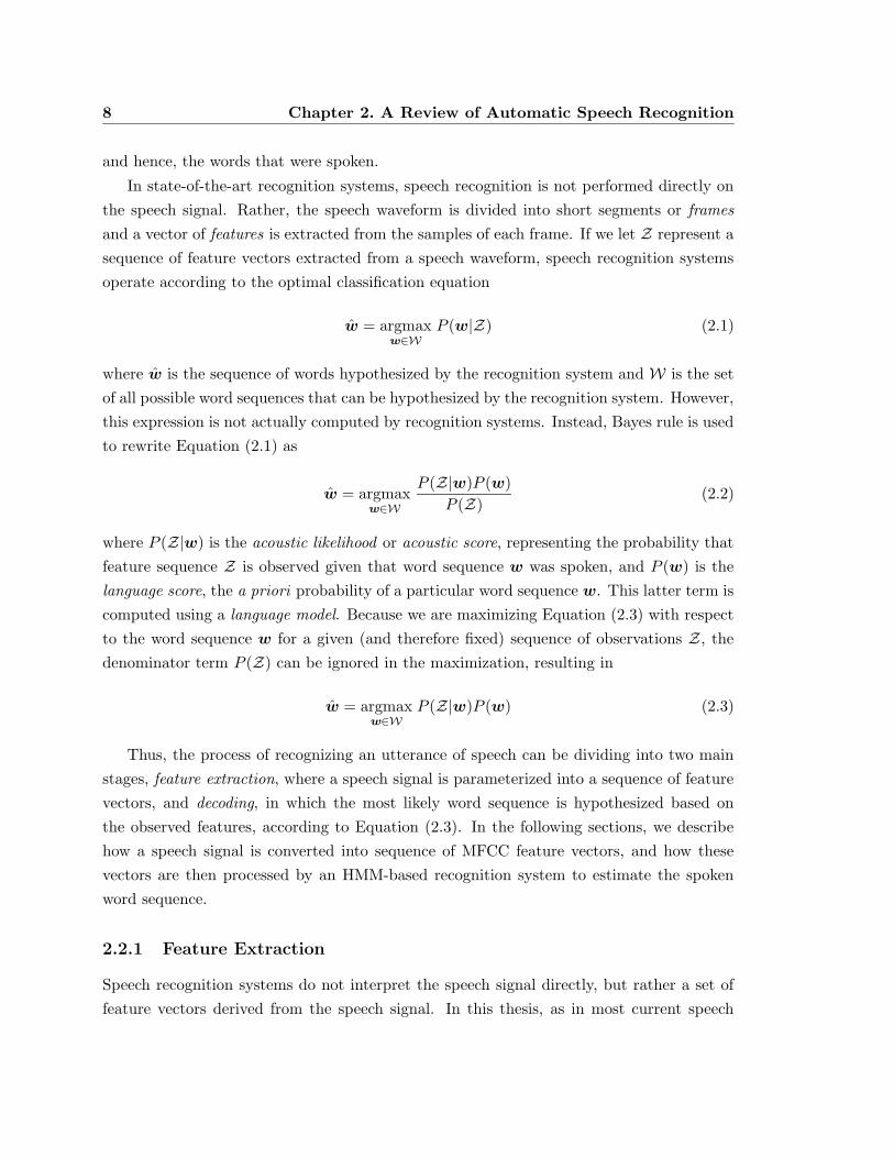
In state-of-the-art recognition systems, speech recognition is not performed directly on
the speech signal. Rather, the speech waveform is divided into short segments or frames
and a vector of features is extracted from the samples of each frame. If we let Z represent a
sequence of feature vectors extracted from a speech waveform, speech recognition systems
operate according to the optimal classification equation
w = argmaxw∈W
P (w|Z) (2.1)
where w is the sequence of words hypothesized by the recognition system and W is the set
of all possible word sequences that can be hypothesized by the recognition system. However,
this expression is not actually computed by recognition systems. Instead, Bayes rule is used
to rewrite Equation (2.1) as
w = argmaxw∈W
P (Z|w)P (w)
P (Z)(2.2)
where P (Z|w) is the acoustic likelihood or acoustic score, representing the probability that
feature sequence Z is observed given that word sequence w was spoken, and P (w) is the
language score, the a priori probability of a particular word sequence w. This latter term is
computed using a language model. Because we are maximizing Equation (2.3) with respect
to the word sequence w for a given (and therefore fixed) sequence of observations Z, the
denominator term P (Z) can be ignored in the maximization, resulting in
w = argmaxw∈W
P (Z|w)P (w) (2.3)
Thus, the process of recognizing an utterance of speech can be dividing into two main
stages, feature extraction, where a speech signal is parameterized into a sequence of feature
vectors, and decoding, in which the most likely word sequence is hypothesized based on
the observed features, according to Equation (2.3). In the following sections, we describe
how a speech signal is converted into sequence of MFCC feature vectors, and how these
vectors are then processed by an HMM-based recognition system to estimate the spoken
word sequence.
2.2.1 Feature Extraction
Speech recognition systems do not interpret the speech signal directly, but rather a set of
feature vectors derived from the speech signal. In this thesis, as in most current speech
2.2. HMM-based Automatic Speech Recognition 9
recognition systems, the speech signal is parameterized into a sequence of vectors called
mel-frequency cepstral coefficients (MFCC) (Davis & Mermelstein, 1980), or simply cepstral
coefficients. Because much of the work in this thesis is concerned with the feature generation
process, we will now examine the derivation of cepstral coefficients in detail.
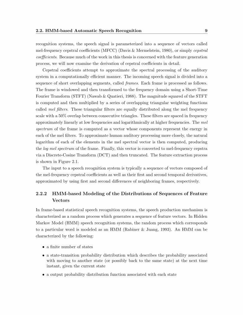
Cepstral coefficients attempt to approximate the spectral processing of the auditory
system in a computationally efficient manner. The incoming speech signal is divided into a
sequence of short overlapping segments, called frames. Each frame is processed as follows.
The frame is windowed and then transformed to the frequency domain using a Short-Time
Fourier Transform (STFT) (Nawab & Quatieri, 1988). The magnitude squared of the STFT
is computed and then multiplied by a series of overlapping triangular weighting functions
called mel filters. These triangular filters are equally distributed along the mel frequency
scale with a 50% overlap between consecutive triangles. These filters are spaced in frequency
approximately linearly at low frequencies and logarithmically at higher frequencies. The mel
spectrum of the frame is computed as a vector whose components represent the energy in
each of the mel filters. To approximate human auditory processing more closely, the natural
logarithm of each of the elements in the mel spectral vector is then computed, producing
the log mel spectrum of the frame. Finally, this vector is converted to mel-frequency cepstra
via a Discrete-Cosine Transform (DCT) and then truncated. The feature extraction process
is shown in Figure 2.1.
The input to a speech recognition system is typically a sequence of vectors composed of
the mel-frequency cepstral coefficients as well as their first and second temporal derivatives,
approximated by using first and second differences of neighboring frames, respectively.
2.2.2 HMM-based Modeling of the Distributions of Sequences of Feature
Vectors
In frame-based statistical speech recognition systems, the speech production mechanism is
characterized as a random process which generates a sequence of feature vectors. In Hidden
Markov Model (HMM) speech recognition systems, the random process which corresponds
to a particular word is modeled as an HMM (Rabiner & Juang, 1993). An HMM can be
characterized by the following:
• a finite number of states
• a state-transition probability distribution which describes the probability associatedwith moving to another state (or possibly back to the same state) at the next timeinstant, given the current state
• a output probability distribution function associated with each state
10 Chapter 2. A Review of Automatic Speech Recognition
STFT
|( )|
log
DCT
� �� �� �� �� �� �� �
� �� �� �� �� �� �� �
WindowHamming
2
Figure 2.1: Flow chart depicting generation of mel-frequency cepstral coefficients from aframe of speech. Typically, a frame size of 25 ms is used, with a frame shift of 10 ms.
2.2. HMM-based Automatic Speech Recognition 11
����� � ����� � ���� ����� �
� ��� � � ��� � � ��� �
�� �� �� �� ��
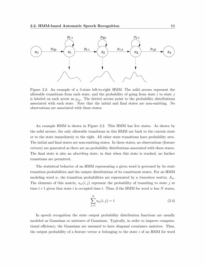
Figure 2.2: An example of a 5-state left-to-right HMM. The solid arrows represent theallowable transitions from each state, and the probability of going from state i to state jis labeled on each arrow as pi|j . The dotted arrows point to the probability distributionsassociated with each state. Note that the initial and final states are non-emitting. Noobservations are associated with these states.
An example HMM is shown in Figure 2.2. This HMM has five states. As shown by
the solid arrows, the only allowable transitions in this HMM are back to the current state
or to the state immediately to the right. All other state transitions have probability zero.
The initial and final states are non-emitting states. In these states, no observations (feature
vectors) are generated as there are no probability distributions associated with these states.
The final state is also an absorbing state, in that when this state is reached, no further
transitions are permitted.
The statistical behavior of an HMM representing a given word is governed by its state
transition probabilities and the output distributions of its constituent states. For an HMM
modeling word w, the transition probabilities are represented by a transition matrix, Aw.
The elements of this matrix, aw(i, j) represent the probability of transiting to state j at
time t+ 1 given that state i is occupied time t. Thus, if the HMM for word w has N states,
N∑
j=1
aw(i, j) = 1 (2.4)
In speech recognition the state output probability distribution functions are usually
modeled as Gaussians or mixtures of Gaussians. Typically, in order to improve computa-
tional efficiency, the Gaussians are assumed to have diagonal covariance matrices. Thus,
the output probability of a feature vector z belonging to the state i of an HMM for word
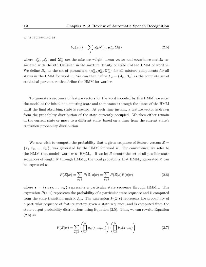
12 Chapter 2. A Review of Automatic Speech Recognition
w, is represented as
bw(z , i) =∑
k
αwikN (z ;µwik,Σwik) (2.5)
where αwik, µwik, and Σw
ik are the mixture weight, mean vector and covariance matrix as-
sociated with the kth Gaussian in the mixture density of state i of the HMM of word w.
We define Bw as the set of parameters {αwik,µwik,Σwik} for all mixture components for all
states in the HMM for word w. We can then define λw = (Aw, Bw) as the complete set of
statistical parameters that define the HMM for word w.
To generate a sequence of feature vectors for the word modeled by this HMM, we enter
the model at the initial non-emitting state and then transit through the states of the HMM
until the final absorbing state is reached. At each time instant, a feature vector is drawn
from the probability distribution of the state currently occupied. We then either remain
in the current state or move to a different state, based on a draw from the current state’s
transition probability distribution.
We now wish to compute the probability that a given sequence of feature vectors Z =
{z1, z2, . . . , zN}, was generated by the HMM for word w. For convenience, we refer to
the HMM that models word w as HMMw. If we let S denote the set of all possible state
sequences of length N through HMMw, the total probability that HMMw generated Z can
be expressed as
P (Z|w) =∑
s∈SP (Z, s|w) =
∑
s∈SP (Z|s)P (s|w) (2.6)
where s = {s1, s2, . . . , sN} represents a particular state sequence through HMMw. The
expression P (s|w) represents the probability of a particular state sequence and is computed
from the state transition matrix Aw. The expression P (Z|s) represents the probability of
a particular sequence of feature vectors given a state sequence, and is computed from the
state output probability distributions using Equation (2.5). Thus, we can rewrite Equation
(2.6) as
P (Z|w) =∑
s∈S
(N∏
t=1
aw(st, st+1)
)(N∏
t=1
bw(zt, st)
)(2.7)
2.2. HMM-based Automatic Speech Recognition 13
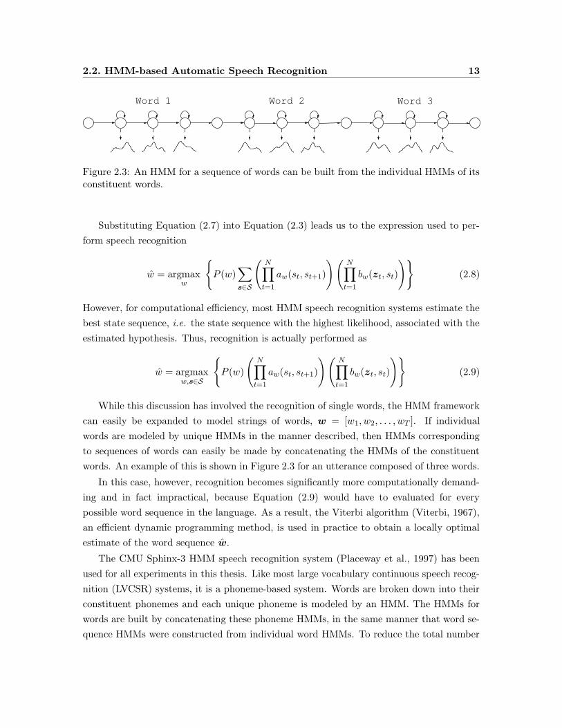
Word 2 Word 3Word 1
Figure 2.3: An HMM for a sequence of words can be built from the individual HMMs of itsconstituent words.
Substituting Equation (2.7) into Equation (2.3) leads us to the expression used to per-
form speech recognition
w = argmaxw
{P (w)
∑
s∈S
(N∏
t=1
aw(st, st+1)
)(N∏
t=1
bw(zt, st)
)}(2.8)
However, for computational efficiency, most HMM speech recognition systems estimate the
best state sequence, i.e. the state sequence with the highest likelihood, associated with the
estimated hypothesis. Thus, recognition is actually performed as
w = argmaxw,s∈S
{P (w)
(N∏
t=1
aw(st, st+1)
)(N∏
t=1
bw(zt, st)
)}(2.9)
While this discussion has involved the recognition of single words, the HMM framework
can easily be expanded to model strings of words, w = [w1, w2, . . . , wT ]. If individual
words are modeled by unique HMMs in the manner described, then HMMs corresponding
to sequences of words can easily be made by concatenating the HMMs of the constituent
words. An example of this is shown in Figure 2.3 for an utterance composed of three words.
In this case, however, recognition becomes significantly more computationally demand-
ing and in fact impractical, because Equation (2.9) would have to evaluated for every
possible word sequence in the language. As a result, the Viterbi algorithm (Viterbi, 1967),
an efficient dynamic programming method, is used in practice to obtain a locally optimal
estimate of the word sequence w.
The CMU Sphinx-3 HMM speech recognition system (Placeway et al., 1997) has been
used for all experiments in this thesis. Like most large vocabulary continuous speech recog-
nition (LVCSR) systems, it is a phoneme-based system. Words are broken down into their
constituent phonemes and each unique phoneme is modeled by an HMM. The HMMs for
words are built by concatenating these phoneme HMMs, in the same manner that word se-
quence HMMs were constructed from individual word HMMs. To reduce the total number
14 Chapter 2. A Review of Automatic Speech Recognition
of parameters needed by the HMMs for all phonemes modeled by the recognition system,
the parameters of the Gaussian distributions are shared across states of various phonemes.
States which share parameters in this manner are called tied states or senones. More infor-
mation on procedures for this parameter sharing can be found in (Hwang & Huang, 1993;
Hwang, 1993).
2.3 ASR Performance in Distant-talking Environments
Speech recognition systems operate on the premise that the distributions which model the
various sound classes are representative of the speech being recognized. That is, there is
an underlying assumption that the test and training data were generated from the same
or very similar distributions. More specifically, a speech recognition system that has been
trained on clean speech can only be expected to perform accurately when the test data
is clean as well. When the test data has been corrupted in some manner, it is no longer
well represented by the statistical models of the recognizer, and as a result, performance
degrades, e.g. (Moreno, 1996). This problem can be alleviated somewhat by subjecting
the training data to the exact same distortion as the test speech, and retraining the speech
recognition system. However, this situation is impractical, as it is difficult, if not impossible
to generate training data in this manner. There is simply too much variability in the
sources and levels of distortion possible in the test speech. In distant-talking environments,
there are two primary sources of distortion which degrade speech recognition performance:
additive noise and reverberation.
2.3.1 The Effect of Additive Noise on Recognition Accuracy
There are several types of noise that can corrupt the speech signal in a distant-talking
environment. Point sources or coherent sources are noise sources with a distinct point of
origin, such as a radio or another talker. Such sources propagate to the microphone in much
the same manner as the speech signal. On the other hand, when noise of approximately
equal energy propagates in all directions at once, a diffuse noise field is created. Offices and
vehicles are examples of environments where diffuse noise fields commonly exist. Finally,
the speech signal can be corrupted by electrical noise in the microphone itself. However, this
type of noise generally produces minimal distortion and has a negligible effect on speech
recognition performance. In distant-talking environments, the microphone is located at
some distance from the user. Because the signal amplitude decays as a function of the
distance traveled (Beranek, 1954), the energy of the direct speech signal at the microphone
2.3. ASR Performance in Distant-talking Environments 15
0 5 10 15 20 25 clean0
20
40
60
80
100
SNR (dB)
Wor
d E
rror
Rat
e (%
)
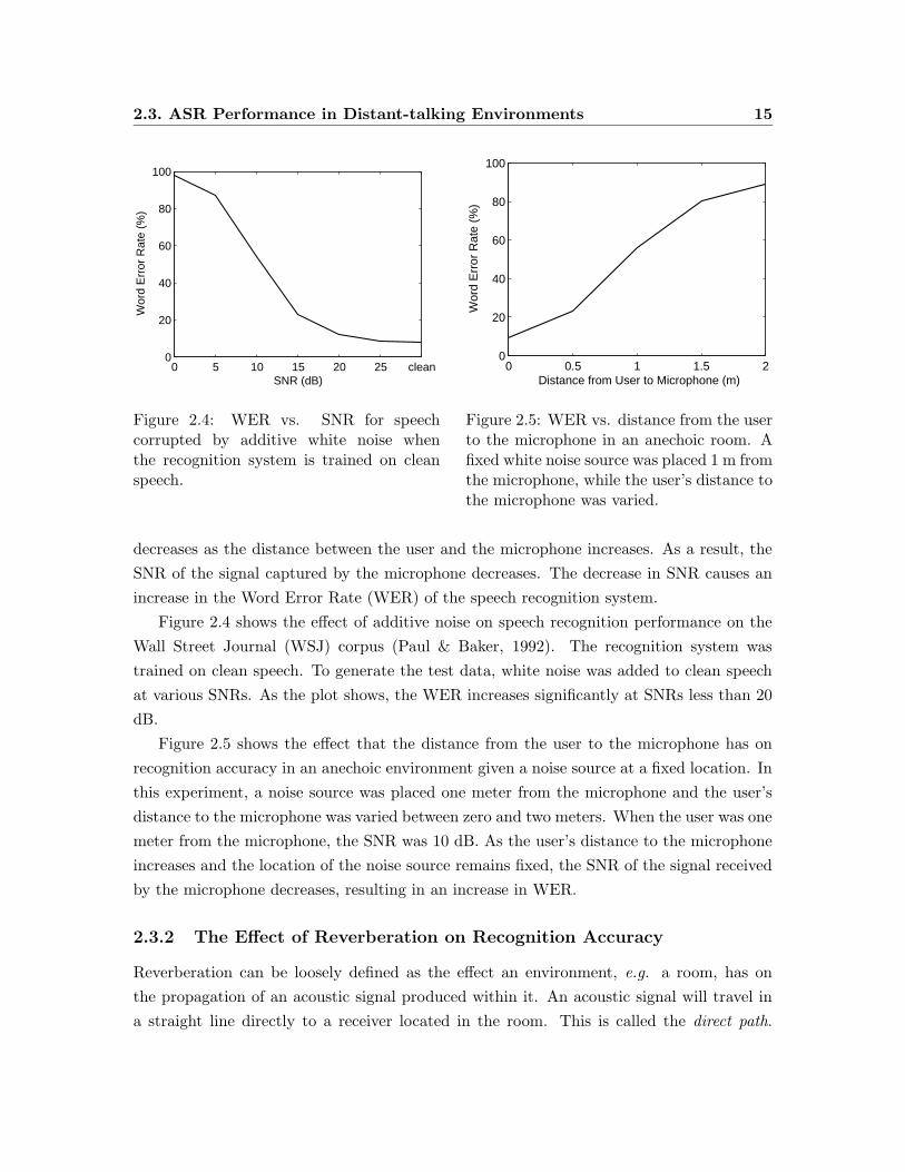
Figure 2.4: WER vs. SNR for speechcorrupted by additive white noise whenthe recognition system is trained on cleanspeech.
0 0.5 1 1.5 20
20
40
60
80
100
Distance from User to Microphone (m)
Wor
d E
rror
Rat
e (%
)
Figure 2.5: WER vs. distance from the userto the microphone in an anechoic room. Afixed white noise source was placed 1 m fromthe microphone, while the user’s distance tothe microphone was varied.
decreases as the distance between the user and the microphone increases. As a result, the
SNR of the signal captured by the microphone decreases. The decrease in SNR causes an
increase in the Word Error Rate (WER) of the speech recognition system.
Figure 2.4 shows the effect of additive noise on speech recognition performance on the
Wall Street Journal (WSJ) corpus (Paul & Baker, 1992). The recognition system was
trained on clean speech. To generate the test data, white noise was added to clean speech
at various SNRs. As the plot shows, the WER increases significantly at SNRs less than 20
dB.
Figure 2.5 shows the effect that the distance from the user to the microphone has on
recognition accuracy in an anechoic environment given a noise source at a fixed location. In
this experiment, a noise source was placed one meter from the microphone and the user’s
distance to the microphone was varied between zero and two meters. When the user was one
meter from the microphone, the SNR was 10 dB. As the user’s distance to the microphone
increases and the location of the noise source remains fixed, the SNR of the signal received
by the microphone decreases, resulting in an increase in WER.
2.3.2 The Effect of Reverberation on Recognition Accuracy
Reverberation can be loosely defined as the effect an environment, e.g. a room, has on
the propagation of an acoustic signal produced within it. An acoustic signal will travel in
a straight line directly to a receiver located in the room. This is called the direct path.
16 Chapter 2. A Review of Automatic Speech Recognition
The signal also propagates in all directions, hitting the various surfaces in the room (walls,
furniture, other sources, etc.). These surfaces absorb some of the signal’s energy and reflect
the rest. The reflected signals arrive at the receiver essentially as delayed and attenuated
copies of the direct-path signal. Although reverberation is a function of many factors,
including the materials covering the surfaces of the room, frequency, temperature, and
other acoustical phenomena, it can be modeled quite effectively as a linear Finite-Impulse-
Response (FIR) filter. We refer to the impulse response of such a filter as the room impulse
response. An acoustic signal propagating in a reverberant environment is therefore well
modeled by convolving the signal with the room impulse response.
The room impulse response can be obtained either by direct measurement or simulation.
The basic method of measuring a room impulse response is to play an impulsive sound from
a loudspeaker, record the signal, and then deconvolve the original and recorded signals
to obtain the impulse response. A commonly used signal for this task is called the time-
stretched pulse (TSP). More information about the TSP and the details of the impulse
response measurement technique can be found in (Suzuki et al., 1995).
Room impulse responses can also be simulated using a technique called the image method
(Allen & Berkley, 1979). This method relies on some strong acoustic assumptions in order
to create a mathematical model of sound reflections in a rectangular enclosure. Specifically,
it assumes that all room surfaces are nearly rigid and the absorption coefficients of the
surface materials are frequency independent. In spite of its shortcomings, the image method
remains a popular and convenient method for simulating a room impulse response because
it requires no actual acoustical measurements and is relatively simple to implement.
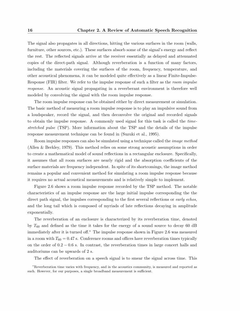
Figure 2.6 shows a room impulse response recorded by the TSP method. The notable
characteristics of an impulse response are the large initial impulse corresponding the the
direct path signal, the impulses corresponding to the first several reflections or early echos,
and the long tail which is composed of myriads of late reflections decaying in amplitude
exponentially.
The reverberation of an enclosure is characterized by its reverberation time, denoted
by T60 and defined as the time it takes for the energy of a sound source to decay 60 dB
immediately after it is turned off.∗ The impulse response shown in Figure 2.6 was measured
in a room with T60 = 0.47 s. Conference rooms and offices have reverberation times typically
on the order of 0.2− 0.6 s. In contrast, the reverberation times in large concert halls and
auditoriums can be upwards of 2 s.
The effect of reverberation on a speech signal is to smear the signal across time. This
∗Reverberation time varies with frequency, and in the acoustics community, is measured and reported assuch. However, for our purposes, a single broadband measurement is sufficient.
2.3. ASR Performance in Distant-talking Environments 17
0 0.02 0.04 0.06 0.08 0.1 0.12
-0.2
-0.1
0
0.1
0.2
0.3
Time (sec)
Am
plitu
de
Early Echos
Direct ResponseLong Decaying Tail
Figure 2.6: The room impulse response from a room with a reverberation time of 0.47 smeasured using the TSP method. Only the first 0.125 s of the impulse response is shownhere in order to highlight the prominent features.
is quite intuitive if one considers that the room impulse response is simply a collection
of delayed and attenuated impulses. The amount of smearing is a function of both the
reverberation time, which generally dictates the length of the room impulse response, and
the signal-to-reverberation ratio (SRR), the ratio of energy in the direct path impulse to
the energy in the remainder of the impulse response. Because of the manner in which
the amplitude of speech decays as a function of distance traveled, the SRR is inversely
proportional to the distance between the source and the receiver.
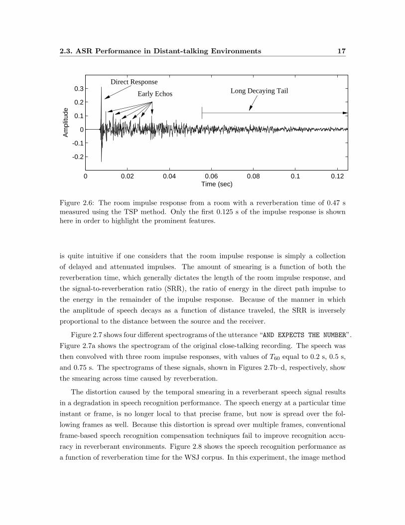
Figure 2.7 shows four different spectrograms of the utterance “AND EXPECTS THE NUMBER”.
Figure 2.7a shows the spectrogram of the original close-talking recording. The speech was
then convolved with three room impulse responses, with values of T60 equal to 0.2 s, 0.5 s,
and 0.75 s. The spectrograms of these signals, shown in Figures 2.7b–d, respectively, show
the smearing across time caused by reverberation.
The distortion caused by the temporal smearing in a reverberant speech signal results
in a degradation in speech recognition performance. The speech energy at a particular time
instant or frame, is no longer local to that precise frame, but now is spread over the fol-
lowing frames as well. Because this distortion is spread over multiple frames, conventional
frame-based speech recognition compensation techniques fail to improve recognition accu-
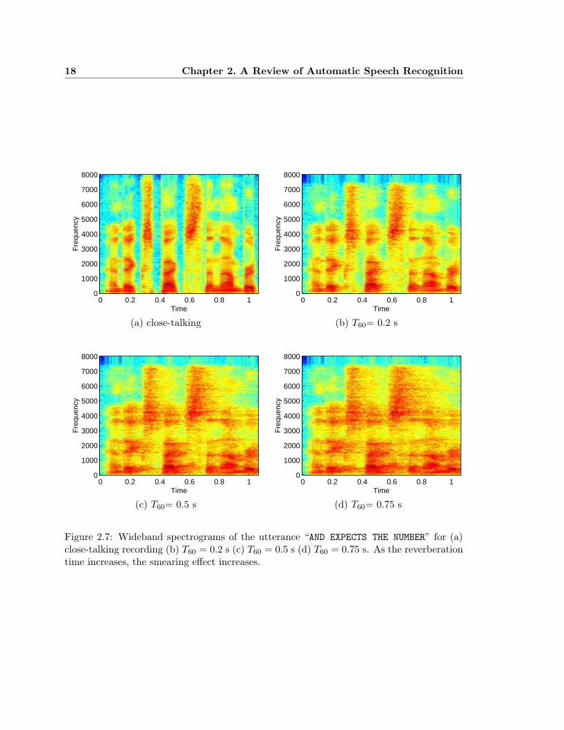
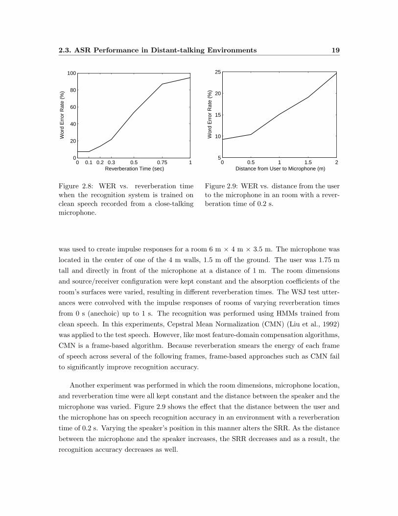
racy in reverberant environments. Figure 2.8 shows the speech recognition performance as
a function of reverberation time for the WSJ corpus. In this experiment, the image method
18 Chapter 2. A Review of Automatic Speech Recognition
Time
Fre
quen
cy
0 0.2 0.4 0.6 0.8 10
1000
2000
3000
4000
5000
6000
7000
8000
Time
Fre
quen
cy
0 0.2 0.4 0.6 0.8 10
1000
2000
3000
4000
5000
6000
7000
8000
(a) close-talking (b) T60= 0.2 s
Time
Fre
quen
cy
0 0.2 0.4 0.6 0.8 10
1000
2000
3000
4000
5000
6000
7000
8000
Time
Fre
quen
cy
0 0.2 0.4 0.6 0.8 10
1000
2000
3000
4000
5000
6000
7000
8000
(c) T60= 0.5 s (d) T60= 0.75 s
Figure 2.7: Wideband spectrograms of the utterance “AND EXPECTS THE NUMBER” for (a)close-talking recording (b) T60 = 0.2 s (c) T60 = 0.5 s (d) T60 = 0.75 s. As the reverberationtime increases, the smearing effect increases.
2.3. ASR Performance in Distant-talking Environments 19
0 0.1 0.2 0.3 0.5 0.75 10
20
40
60
80
100
Reverberation Time (sec)
Wor
d E
rror
Rat
e (%
)
Figure 2.8: WER vs. reverberation timewhen the recognition system is trained onclean speech recorded from a close-talkingmicrophone.
0 0.5 1 1.5 25
10
15
20
25
Distance from User to Microphone (m)
Wor
d E
rror
Rat
e (%
)
Figure 2.9: WER vs. distance from the userto the microphone in an room with a rever-beration time of 0.2 s.
was used to create impulse responses for a room 6 m × 4 m × 3.5 m. The microphone was
located in the center of one of the 4 m walls, 1.5 m off the ground. The user was 1.75 m
tall and directly in front of the microphone at a distance of 1 m. The room dimensions
and source/receiver configuration were kept constant and the absorption coefficients of the
room’s surfaces were varied, resulting in different reverberation times. The WSJ test utter-
ances were convolved with the impulse responses of rooms of varying reverberation times
from 0 s (anechoic) up to 1 s. The recognition was performed using HMMs trained from
clean speech. In this experiments, Cepstral Mean Normalization (CMN) (Liu et al., 1992)
was applied to the test speech. However, like most feature-domain compensation algorithms,
CMN is a frame-based algorithm. Because reverberation smears the energy of each frame
of speech across several of the following frames, frame-based approaches such as CMN fail
to significantly improve recognition accuracy.
Another experiment was performed in which the room dimensions, microphone location,
and reverberation time were all kept constant and the distance between the speaker and the
microphone was varied. Figure 2.9 shows the effect that the distance between the user and
the microphone has on speech recognition accuracy in an environment with a reverberation
time of 0.2 s. Varying the speaker’s position in this manner alters the SRR. As the distance
between the microphone and the speaker increases, the SRR decreases and as a result, the
recognition accuracy decreases as well.
20 Chapter 2. A Review of Automatic Speech Recognition
2.4 Summary
In this chapter, the basic operations of an HMM-based speech recognition system have
been described. The feature extraction process, by which an incoming speech waveform is
converted into a series of MFCC vectors, was described in detail. We then saw how Hidden
Markov Models are used to model the distributions of sequences of feature vectors, and how
such models can be used to obtain an estimate of the words spoken based on an observed
sequence of feature vectors. We then considered the performance of speech recognition
systems in distant-talking environments, and showed how recognition accuracy degrades
significantly when the speech is distorted by additive noise and reverberation.
In the next chapter, we will discuss how the use of an array of microphones can improve
the quality of the received speech signal in distant-talking environments.
Chapter 3
An Introduction to Microphone
Array Processing for Speech
Recognition
3.1 Introduction
As discussed in the previous chapter, speech signals captured by a microphone located
away from the user can be significantly corrupted by additive noise and reverberation. One
method of reducing the signal distortion and improving the quality of the signal is to use
multiple microphones rather than a single microphone. Array processing refers to the joint
processing of signals captured by multiple spatially-separated sensors. Array processing is a
relatively mature field, developed initially to process narrowband signals for radar and sonar
applications, and then later applied to broadband signals such as speech. More recently,
the demand for hands-free speech communication and recognition has increased and as a
result, newer techniques have been developed to address the specific issues involved in the
enhancement of speech signals captured by a microphone array.
In this chapter, we present a brief overview of microphone array processing and show how
it can help reduce the distortion of signals captured in distant-talking scenarios. The major
families of array processing methods are described, with specific emphasis on their benefits
and drawbacks when used for speech recognition applications. In addition, we discuss some
single-channel speech recognition compensation algorithms that have been applied to the
output of a microphone array in order to improve the recognition accuracy.
We also use this chapter to introduce the experimental framework used to evaluate the
algorithms presented in this thesis. The speech databases and the speech recognition system
21
22 Chapter 3. Microphone Array Processing for Speech Recognition
used in this thesis are described in detail. Finally, some of the array processing methods
described in this chapter are evaluted through a series of speech recognition experiments.
3.2 Fundamentals of Array Processing
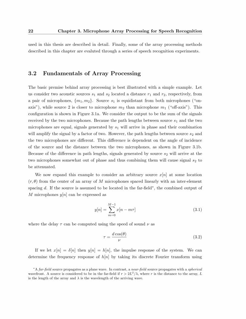
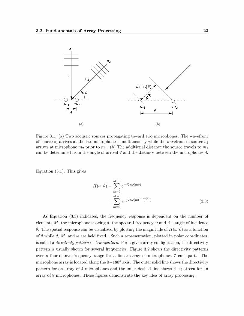
The basic premise behind array processing is best illustrated with a simple example. Let
us consider two acoustic sources s1 and s2 located a distance r1 and r2, respectively, from
a pair of microphones, {m1,m2}. Source s1 is equidistant from both microphones (“on-
axis”), while source 2 is closer to microphone m2 than microphone m1 (“off-axis”). This
configuration is shown in Figure 3.1a. We consider the output to be the sum of the signals
received by the two microphones. Because the path lengths between source s1 and the two
microphones are equal, signals generated by s1 will arrive in phase and their combination
will amplify the signal by a factor of two. However, the path lengths between source s2 and
the two microphones are different. This difference is dependent on the angle of incidence
of the source and the distance between the two microphones, as shown in Figure 3.1b.
Because of the difference in path lengths, signals generated by source s2 will arrive at the
two microphones somewhat out of phase and thus combining them will cause signal s2 to
be attenuated.
We now expand this example to consider an arbitrary source x[n] at some location
(r, θ) from the center of an array of M microphones spaced linearly with an inter-element
spacing d. If the source is assumed to be located in the far-field∗, the combined output of
M microphones y[n] can be expressed as
y[n] =M−1∑
m=0
x[n−mτ ] (3.1)
where the delay τ can be computed using the speed of sound ν as
τ =d cos(θ)
ν(3.2)
If we let x[n] = δ[n] then y[n] = h[n], the impulse response of the system. We can
determine the frequency response of h[n] by taking its discrete Fourier transform using
∗A far-field source propagates as a plane wave. In contrast, a near-field source propagates with a sphericalwavefront. A source is considered to be in the far-field if r > 2L2/λ, where r is the distance to the array, Lis the length of the array and λ is the wavelength of the arriving wave.
3.2. Fundamentals of Array Processing 23
���
���
��� ���
���
���
(a)
��� ���
�������������
�
(b)
Figure 3.1: (a) Two acoustic sources propagating toward two microphones. The wavefrontof source s1 arrives at the two microphones simultaneously while the wavefront of source s2
arrives at microphone m2 prior to m1. (b) The additional distance the source travels to m1
can be determined from the angle of arrival θ and the distance between the microphones d.
Equation (3.1). This gives
H(ω, θ) =M−1∑
m=0
e−j2πω(mτ)
=M−1∑
m=0
e−j2πω(m(d cos(θ)
ν) (3.3)
As Equation (3.3) indicates, the frequency response is dependent on the number of
elements M , the microphone spacing d, the spectral frequency ω and the angle of incidence
θ. The spatial response can be visualized by plotting the magnitude of H(ω, θ) as a function
of θ while d, M , and ω are held fixed . Such a representation, plotted in polar coordinates,
is called a directivity pattern or beampattern. For a given array configuration, the directivity
pattern is usually shown for several frequencies. Figure 3.2 shows the directivity patterns
over a four-octave frequency range for a linear array of microphones 7 cm apart. The
microphone array is located along the 0−180◦ axis. The outer solid line shows the directivity
pattern for an array of 4 microphones and the inner dashed line shows the pattern for an
array of 8 microphones. These figures demonstrate the key idea of array processing:
24 Chapter 3. Microphone Array Processing for Speech Recognition
0.2
0.4
0.6
0.8
1
30
210
60
240
90
270
120
300
150
330
180 0
0.2
0.4
0.6
0.8
1
30
210
60
240
90
270
120
300
150
330
180 0
(a) 400 Hz (b) 800 Hz
0.2
0.4
0.6
0.8
1
30
210
60
240
90
270
120
300
150
330
180 0
0.2
0.4
0.6
0.8
1
30
210
60
240
90
270
120
300
150
330
180 0
(c) 1600 Hz (d) 3200 Hz
Figure 3.2: The directivity patterns of a linear microphone array over a four octave fre-quency range. The solid outer plots show the directivity patterns of a 4-element array whilethe dashed inner plots correspond to an 8-element array. In both cases, the inter-elementspacing is 7 cm.

3.2. Fundamentals of Array Processing 25
0.2
0.4
0.6
0.8
1
30
210
60
240
90
270
120
300
150
330
180 0
0.2
0.4
0.6
0.8
1
30
210
60
240
90
270
120
300
150
330
180 0
(a) 4800 Hz (b) 6400 Hz
Figure 3.3: The beampatterns for the same microphone array configurations used in Figure3.2 at frequencies which violate the spatial sampling theorem. The large unwanted sidelobesare the result of spatial aliasing.
By using an array of microphones rather than a single microphone, we are able to
achieve spatial selectivity, reinforcing sources propagating from a particular direction, while
attenuating sources propagating from other directions.
It is apparent from examining the beampatterns that this “spatial selectivity” varies as
a function of frequency. A linear array generally has a wide beamwidth at low frequencies,
which narrows as the frequency increases. An array of microphones essentially samples the
sound field at different points in space. As a result, array processing is subject to a spatial
analog of temporal aliasing that occurs when signals are sampled too slowly. When spatial
aliasing occurs, the array is unable to distinguish between multiple arrival angles for a
given frequency and large sidelobes appear in unwanted directions, as shown in Figure 3.3.
To prevent spatial aliasing in linear arrays, the spatial sampling theorem must be followed,
which states that if λmin is the minimum wavelength of interest and d is the microphone
spacing, then d < λmin/2 (Johnson & Dudgeon, 1993). Spatial aliasing can also be avoided
by using a nested harmonic array (Flanagan et al., 1985) or a “randomly distributed” array.
26 Chapter 3. Microphone Array Processing for Speech Recognition
3.3 Microphone Array Processing Approaches
3.3.1 Classical Beamforming
The concept of algorithmically steering the main lobe or beam of a directivity pattern in a
desired direction is called beamforming. The direction the array is steered is called the look
direction. In order to steer an array of arbitrary configuration and number of sensors, the
signals received by the array are first delayed to compensate for the path length differences
from the source to the various microphones and then the signals are combined together.
This technique, appropriately known as delay-and-sum beamforming, can be mathematically
expressed simply as
y[n] =M−1∑
m=0
αmxm[n− τm] (3.4)
where αm is a weight applied to the signal received by microphone m. There are several
methods for choosing the weights α0 . . . αM−1. The simplest and most common method
is to set them all equal to 1/M . This technique simply averages the time-aligned signals
and is referred to as unweighted delay-and-sum beamforming. The process of finding the
delays is known as time-delay estimation (TDE) and is closely related to the problem of
source localization. Many TDE methods exist in the literature, and most are based on
cross-correlation. More information about TDE and source localization for speech signals
can be found in (Brandstein & Ward, 2001). It can be shown that if the noise signals
corrupting each microphone channel are uncorrelated to each other and the target signal,
delay-and-sum processing results in a 3 dB increase in the SNR of the output signal for every
doubling of the number of microphones in the array (Johnson & Dudgeon, 1993). Many
microphone-array-based speech recognition systems have successfully used delay-and-sum
processing to improve recognition performance, and because of its simplicity, it remains the
method of choice for many array-based speech recognition systems, e.g. (Omologo et al.,
1997; Hughes et al., 1999). The delay-and-sum beamformer can be generalized to a filter-
and-sum beamformer where rather than a single weight, each microphone signal has an
associated filter and the captured signals are filtered before they are combined. Filter-and-
sum beamforming can be expressed as
y[n] =M−1∑
m=0
P−1∑
p=0
hm[p]xm[n− p− τm] (3.5)
3.3. Microphone Array Processing Approaches 27
where hm[p] is the pth tap of the filter associated with microphone m. Clearly, delay-and-
sum processing is simply filter-and-sum with a 1-tap filter for each microphone.
Both the delay-and-sum and filter-and-sum methods are examples of fixed beamforming
algorithms, as the array processing parameters do not change dynamically over time. If
the source moves then the delay values will of course change, but these algorithms are
still considered fixed parameter algorithms. In the next section, we give a brief overview
of adaptive array processing methods, where parameters are time-varying and adjusted to
track changes in the target signal and environment.
3.3.2 Adaptive Array Processing
In adaptive beamforming, the array-processing parameters are dynamically adjusted accord-
ing to some optimization criterion, either on a sample-by-sample or on a frame-by-frame
basis. The Frost algorithm (1972) is arguably the most well-known adaptive beamforming
technique. This algorithm is a constrained LMS algorithm in which filter taps (weights)
applied to each signal in the array are adaptively adjusted to minimize the output power
of the array while maintaining a desired frequency response in the look direction.
Griffiths and Jim (1982) proposed the Generalized Sidelobe Canceller (GSC) as an alter-
native architecture for the Frost beamformer. The GSC consists of two structures, a fixed
beamformer which produces a non-adaptive output and an adaptive structure for sidelobe
cancellation. The adaptive structure of the GSC is preceded by a blocking matrix which
blocks signals coming from the look direction. The weights of the adaptive structure are
then adjusted to cancel any signal common to both structures. The architecture of the
Griffiths-Jim GSC is shown in Figure 3.4.
In some cases, the filter parameters can be calibrated to a particular environment or
user. For example, Nordholm et al. (1999) proposed a calibration scheme designed for a
hands-free telephone environment in an automobile. A series of typical target signals from
the speaker, as well as jammer signals from the hands-free loudspeaker, are captured in
the car and used for initial calibration of the parameters of a filter-and-sum beamforming
system. These parameters are then adapted during use based on the stored calibration
signals and updated noise estimates.
Adaptive-filter methods generally assume that the target and jammer signals are un-
correlated. When this assumption is violated, as is the case for speech in a reverberant
environment, the methods suffer from signal cancellation because reflected copies of the
target signal appear as unwanted jammer signals. This seriously degrades the quality of the
output signal and results in poor speech recognition performance. Van Compernolle (1990)
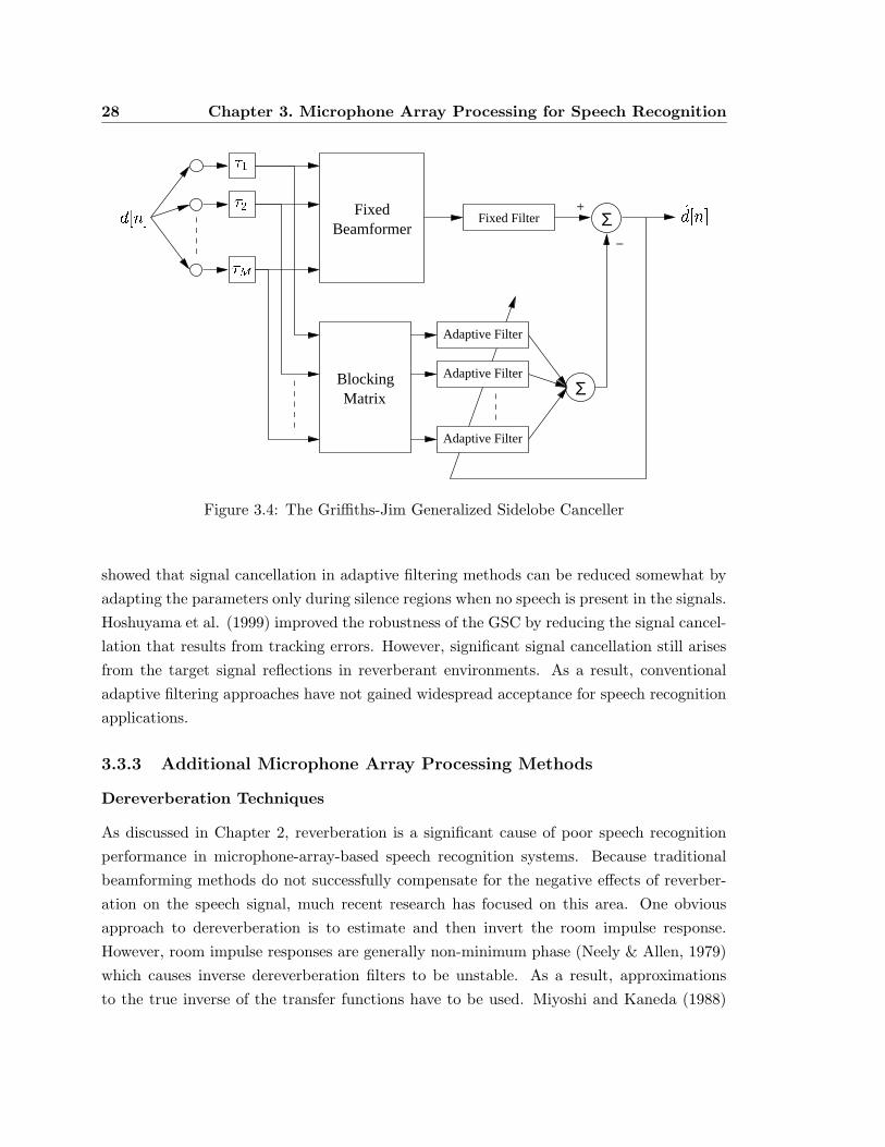
28 Chapter 3. Microphone Array Processing for Speech Recognition
Fixed FilterFixed
Beamformer
BlockingMatrix
Adaptive Filter
Adaptive Filter
Adaptive Filter
Σ
Σ+
−
���
���
���
���� �����
Figure 3.4: The Griffiths-Jim Generalized Sidelobe Canceller
showed that signal cancellation in adaptive filtering methods can be reduced somewhat by
adapting the parameters only during silence regions when no speech is present in the signals.
Hoshuyama et al. (1999) improved the robustness of the GSC by reducing the signal cancel-
lation that results from tracking errors. However, significant signal cancellation still arises
from the target signal reflections in reverberant environments. As a result, conventional
adaptive filtering approaches have not gained widespread acceptance for speech recognition
applications.
3.3.3 Additional Microphone Array Processing Methods
Dereverberation Techniques
As discussed in Chapter 2, reverberation is a significant cause of poor speech recognition
performance in microphone-array-based speech recognition systems. Because traditional
beamforming methods do not successfully compensate for the negative effects of reverber-
ation on the speech signal, much recent research has focused on this area. One obvious
approach to dereverberation is to estimate and then invert the room impulse response.
However, room impulse responses are generally non-minimum phase (Neely & Allen, 1979)
which causes inverse dereverberation filters to be unstable. As a result, approximations
to the true inverse of the transfer functions have to be used. Miyoshi and Kaneda (1988)
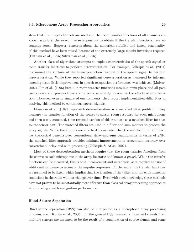
3.3. Microphone Array Processing Approaches 29
show that if multiple channels are used and the room transfer functions of all channels are
known a priori , the exact inverse is possible to obtain if the transfer functions have no
common zeros. However, concerns about the numerical stability and hence, practicality,
of this method have been raised because of the extremely large matrix inversions required
(Putnam et al., 1995; Silverman et al., 1996).
Another class of algorithms attempts to exploit characteristics of the speech signal or
room transfer functions to perform dereverberation. For example, Gillespie et al. (2001)
maximized the kurtosis of the linear prediction residual of the speech signal to perform
dereverberation. While they reported significant dereverberation as measured by informal
listening tests, little improvement in speech recognition performance was achieved (Malvar,
2002). Liu et al. (1996) break up room transfer functions into minimum phase and all-pass
components and process these components separately to remove the effects of reverbera-
tion. However, even in simulated environments, they report implementation difficulties in
applying this method to continuous speech signals.
Flanagan et al. (1993) approach dereverberation as a matched filter problem. They
measure the transfer function of the source-to-sensor room response for each microphone
and then use a truncated, time-reversed version of this estimate as a matched-filter for that
source-sensor pair. The matched filters are used in a filter-and-sum manner to process the
array signals. While the authors are able to demonstrated that the matched filter approach
has theoretical benefits over conventional delay-and-sum beamforming in terms of SNR,
the matched filter approach provides minimal improvements in recognition accuracy over
conventional delay-and-sum processing (Gillespie & Atlas, 2002).
Most of these dereverberation methods require that the room transfer functions from
the source to each microphone in the array be static and known a priori . While the transfer
functions can be measured, this is both inconvenient and unrealistic, as it requires the use of
additional hardware to estimate the impulse responses. Furthermore, the transfer functions
are assumed to be fixed, which implies that the location of the talker and the environmental
conditions in the room will not change over time. Even with such knowledge, these methods
have not proven to be substantially more effective than classical array processing approaches
at improving speech recognition performance.
Blind Source Separation
Blind source separation (BSS) can also be interpreted as a microphone array processing
problem, e.g. (Kurita et al., 2000). In the general BSS framework, observed signals from
multiple sensors are assumed to be the result of a combination of source signals and some
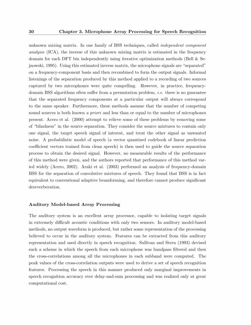
30 Chapter 3. Microphone Array Processing for Speech Recognition
unknown mixing matrix. In one family of BSS techniques, called independent component
analysis (ICA), the inverse of this unknown mixing matrix is estimated in the frequency
domain for each DFT bin independently using iterative optimization methods (Bell & Se-
jnowski, 1995). Using this estimated inverse matrix, the microphone signals are “separated”
on a frequency-component basis and then recombined to form the output signals. Informal
listenings of the separation produced by this method applied to a recording of two sources
captured by two microphones were quite compelling. However, in practice, frequency-
domain BSS algorithms often suffer from a permutation problem, i.e. there is no guarantee
that the separated frequency components at a particular output will always correspond
to the same speaker. Furthermore, these methods assume that the number of competing
sound sources is both known a priori and less than or equal to the number of microphones
present. Acero et al. (2000) attempt to relieve some of these problems by removing some
of “blindness” in the source separation. They consider the source mixtures to contain only
one signal, the target speech signal of interest, and treat the other signal as unwanted
noise. A probabilistic model of speech (a vector quantized codebook of linear prediction
coefficient vectors trained from clean speech) is then used to guide the source separation
process to obtain the desired signal. However, no measurable results of the performance
of this method were given, and the authors reported that performance of this method var-
ied widely (Acero, 2002). Araki et al. (2003) performed an analysis of frequency-domain
BSS for the separation of convolutive mixtures of speech. They found that BSS is in fact
equivalent to conventional adaptive beamforming, and therefore cannot produce significant
dereverberation.
Auditory Model-based Array Processing
The auditory system is an excellent array processor, capable to isolating target signals
in extremely difficult acoustic conditions with only two sensors. In auditory model-based
methods, no output waveform is produced, but rather some representation of the processing
believed to occur in the auditory system. Features can be extracted from this auditory
representation and used directly in speech recognition. Sullivan and Stern (1993) devised
such a scheme in which the speech from each microphone was bandpass filtered and then
the cross-correlations among all the microphones in each subband were computed. The
peak values of the cross-correlation outputs were used to derive a set of speech recognition
features. Processing the speech in this manner produced only marginal improvements in
speech recognition accuracy over delay-and-sum processing and was realized only at great
computational cost.
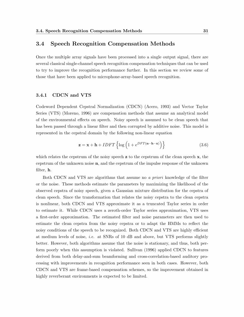
3.4. Speech Recognition Compensation Methods 31
3.4 Speech Recognition Compensation Methods
Once the multiple array signals have been processed into a single output signal, there are
several classical single-channel speech recognition compensation techniques that can be used
to try to improve the recognition performance further. In this section we review some of
those that have been applied to microphone-array-based speech recognition.
3.4.1 CDCN and VTS
Codeword Dependent Cepstral Normalization (CDCN) (Acero, 1993) and Vector Taylor
Series (VTS) (Moreno, 1996) are compensation methods that assume an analytical model
of the environmental effects on speech. Noisy speech is assumed to be clean speech that
has been passed through a linear filter and then corrupted by additive noise. This model is
represented in the cepstral domain by the following non-linear equation
z = x + h + IDFT{
log(
1 + eDFT (n−h−x))}
(3.6)
which relates the cepstrum of the noisy speech z to the cepstrum of the clean speech x, the
cepstrum of the unknown noise n, and the cepstrum of the impulse response of the unknown
filter, h.
Both CDCN and VTS are algorithms that assume no a priori knowledge of the filter
or the noise. These methods estimate the parameters by maximizing the likelihood of the
observed cepstra of noisy speech, given a Gaussian mixture distribution for the cepstra of
clean speech. Since the transformation that relates the noisy cepstra to the clean cepstra
is nonlinear, both CDCN and VTS approximate it as a truncated Taylor series in order
to estimate it. While CDCN uses a zeroth-order Taylor series approximation, VTS uses
a first-order approximation. The estimated filter and noise parameters are then used to
estimate the clean cepstra from the noisy cepstra or to adapt the HMMs to reflect the
noisy conditions of the speech to be recognized. Both CDCN and VTS are highly efficient
at medium levels of noise, i.e. at SNRs of 10 dB and above, but VTS performs slightly
better. However, both algorithms assume that the noise is stationary, and thus, both per-
form poorly when this assumption is violated. Sullivan (1996) applied CDCN to features
derived from both delay-and-sum beamforming and cross-correlation-based auditory pro-
cessing with improvements in recognition performance seen in both cases. However, both
CDCN and VTS are frame-based compensation schemes, so the improvement obtained in
highly reverberant environments is expected to be limited.
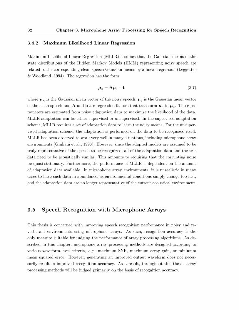
32 Chapter 3. Microphone Array Processing for Speech Recognition
3.4.2 Maximum Likelihood Linear Regression
Maximum Likelihood Linear Regression (MLLR) assumes that the Gaussian means of the
state distributions of the Hidden Markov Models (HMM) representing noisy speech are
related to the corresponding clean speech Gaussian means by a linear regression (Leggetter
& Woodland, 1994). The regression has the form
µn = Aµc + b (3.7)
where µn is the Gaussian mean vector of the noisy speech, µc is the Gaussian mean vector
of the clean speech and A and b are regression factors that transform µc to µn. These pa-
rameters are estimated from noisy adaptation data to maximize the likelihood of the data.
MLLR adaptation can be either supervised or unsupervised. In the supervised adaptation
scheme, MLLR requires a set of adaptation data to learn the noisy means. For the unsuper-
vised adaptation scheme, the adaptation is performed on the data to be recognized itself.
MLLR has been observed to work very well in many situations, including microphone array
environments (Giuliani et al., 1998). However, since the adapted models are assumed to be
truly representative of the speech to be recognized, all of the adaptation data and the test
data need to be acoustically similar. This amounts to requiring that the corrupting noise
be quasi-stationary. Furthermore, the performance of MLLR is dependent on the amount
of adaptation data available. In microphone array environments, it is unrealistic in many
cases to have such data in abundance, as environmental conditions simply change too fast,
and the adaptation data are no longer representative of the current acoustical environment.
3.5 Speech Recognition with Microphone Arrays
This thesis is concerned with improving speech recognition performance in noisy and re-
verberant environments using microphone arrays. As such, recognition accuracy is the
only measure suitable for judging the performance of array processing algorithms. As de-
scribed in this chapter, microphone array processing methods are designed according to
various waveform-level criteria, e.g. maximum SNR, maximum array gain, or minimum
mean squared error. However, generating an improved output waveform does not neces-
sarily result in improved recognition accuracy. As a result, throughout this thesis, array
processing methods will be judged primarily on the basis of recognition accuracy.
3.5. Speech Recognition with Microphone Arrays 33
3.5.1 Experimental Setup and Corpora
Throughout this thesis, Sphinx-3, an HMM-based large-vocabulary speech recognition sys-
tem (Placeway et al., 1997), was used for all speech recognition experiments. The system was
trained using the speaker-independent WSJ training set, which consists of 7000 utterances.
The system was trained using 39-dimensional feature vectors consisting of 13-dimensional
MFCC parameters, along with their delta and delta-delta parameters, computed as de-
scribed in Section 2.2.1. A 25-ms window duration and a frame rate of 100 frames per
second, corresponding to a 10-ms frame shift, were used. Context-dependent 3-state left-
to-right HMMs with no skips were trained and each state distribution was modeled by a
mixture of 8 Gaussians. The system had a total of 4000 senones. Cepstral mean normal-
ization (CMN) was performed on the training utterances.
In order to test recognition performance under a variety of noise and reverberation
conditions, a variety of microphone array corpora were used for the experiments in this
thesis.
CMU 8-Microphone Linear Array Corpus
This corpus, hereafter referred to as “CMU-8”, was recorded by Sullivan (1996) in the
CMU Robust Speech Recognition Laboratory. The utterances were recorded by a linear
microphone array with 8 elements spaced 7 cm apart. The array was placed on a desk and
the user was seated directly in front of the array at a distance of 1 m. Each user wore a
close-talking microphone during the recording, so each array recording has a corresponding
clean control recording. The sampling rate for the recording was 16 kHz. The laboratory
had multiple noise sources, including several computer fans and overhead air blowers. The
reverberation time of the room was measure to be 240 ms. The average SNR of the record-
ings is 6.5 dB. The corpus consists of 140 utterances (10 speakers × 14 utterances). The
utterances consist of strings of keywords as well as alphanumeric strings, where the user
spelled out answers to various census questions, e.g. name, address, etc. Speech recognition
was performed using a flat unigram language model. While the vocabulary size of this
corpus is small (138 words), it is nevertheless a challenging recognition task for two reasons.
First, recognition is performed without the use of any linguistic or syntactic information.
Second, the vocabulary consists of many acoustically confusable words.
ATR Reverberant 7-Microphone Linear Array Corpus
Researchers from ATR in Japan created a microphone array database consisting of room
impulse responses recorded in several different rooms of varying size and reverberation times
34 Chapter 3. Microphone Array Processing for Speech Recognition
using a 14-channel linear array and a 16-channel circular array (Nakamura et al., 2000).
The recordings were made using the TSP method described in Section 2.3.2.
These impulse responses were used to create reverberant WSJ corpora by convolving
the utterances from the WSJ test set with the impulse responses from 7 channels of the
linear array. Five test sets, with T60 from 0.3 to 1.3 s were created. In all cases, the spacing
between the microphones was 5.66 cm and the speaker was directly in front of the array
at a distance of 2 m. The sampling rate was 16 kHz. The WSJ test set has a 5000 word
vocabulary. Recognition was performed using a trigram language model. These corpora
will be referred to as WSJT60 with a subscript indicating the reverberation time, e.g. the
corpus from a room with T60 = 0.3 s will be referred to as WSJ0.3.
3.5.2 Evaluating Performance and Determining Statistical Significance
The merit of the various array processing algorithms presented in this thesis will be judged
primarily by comparing the speech recognition accuracy obtained using these methods to
that obtained using a conventional array processing algorithm. Recognition accuracy is
determined by comparing the word string generated by the recognizer, i.e. the hypothesis,
to the word string actually spoken by the user, i.e. the reference, using a non-linear string
matching program. The Word Error Rate (WER) is computed as ratio of the total number
of errors, including insertions, deletions, and substitutions, to the total number of tokens
in the reference transcription.
When speech recognition accuracy is used as the means of comparing two algorithms, it
is important to verify that any apparent difference in the performance of the two algorithms
is statistically significant. Several methods of evaluating statistical significance for speech
recognition applications have been proposed. One widely accepted method for doing so is
the Matched-Pairs test proposed by Gillick and Cox (1989), which assumes that recognition
errors are independent across speech segments, but not within each segment. This method
has been adopted by the National Institute of Standards and Technology (NIST) for use in
standard speech recognition evaluations, and is the method we use in this thesis as well.
The statistical significance of a particular outcome is dependent on many factors includ-
ing the difference in the error rates of the competing algorithms, the number of segments
or utterances in the test set, the size of the vocabulary, the grammar, and the overall range
of accuracy. Except where noted, the results in this thesis are statistically significant with
p ≤ 0.01.
3.5. Speech Recognition with Microphone Arrays 35
3.5.3 Recognition Results
The first series of experiments was performed on the CMU-8 corpus to determine the recog-
nition accuracy obtained using conventional delay-and-sum beamforming. For each utter-
ance, the array signals were upsampled by a factor of 3 to increase temporal resolution
and the delays in each channel were estimated using the Phase Transform (PHAT) method
(Knapp & Carter, 1976). The channels were then aligned based on the estimated delays
and downsampled to their original sampling rate. The aligned channels were then averaged
to generate the unweighted delay-and-sum output signal. MFCC feature vectors were then
extracted from the output signal and passed to the recognition system for decoding. CMN
was applied to the feature vectors prior to decoding. Experiments were performed using 2,
4, and 8 channels of the array.
Additionally, experiments were performed using the Griffiths-Jim GSC. As expected,
when the adaptation was performed continuously, the algorithm produced a severely dis-
torted output signal due to signal cancellation and the recognition performance was sig-
nificantly worse than even single-channel recognition. When the adaptation was only per-
formed during the silence segments, as suggested by Van Compernolle (1990), performance
improved, but even with a large number of filter parameters, the performance was only
marginally better than delay-and-sum processing.
Figure 3.5 shows the word error rate (WER) for the CMU-8 corpus with only a single
channel and with delay-and-sum beamforming using 2, 4, and 8 array channels. The figure
also shows the performance of using the GSC method with all 8 channels when 50 and 200
taps are used in the adaptive filters. The performance did not improve when more taps were
used. The performance using the close-talking microphone, indicating the upper bound on
performance, is shown as well.
As the figure indicates, microphone array processing provides a significant improvement
in recognition accuracy over a single channel alone. However, while performing delay-and-
sum beamforming on 8 channels is able to reduce the relative WER by more than 40%
compared to a single channel, the performance is still more than 100% worse than that
obtained with a close-talking microphone. Furthermore, it is apparent that adaptive array
processing algorithms, such as the GSC, which depend on the assumption that the signals
coming from directions other than the look direction are uncorrelated with the target signal
do not improve speech recognition over classical delay-and-sum beamforming, and in fact
often perform worse.
These experiments were repeated for the reverberant WSJ corpora. Based on the pre-
vious results, only delay-and-sum beamforming was performed. The results for these ex-
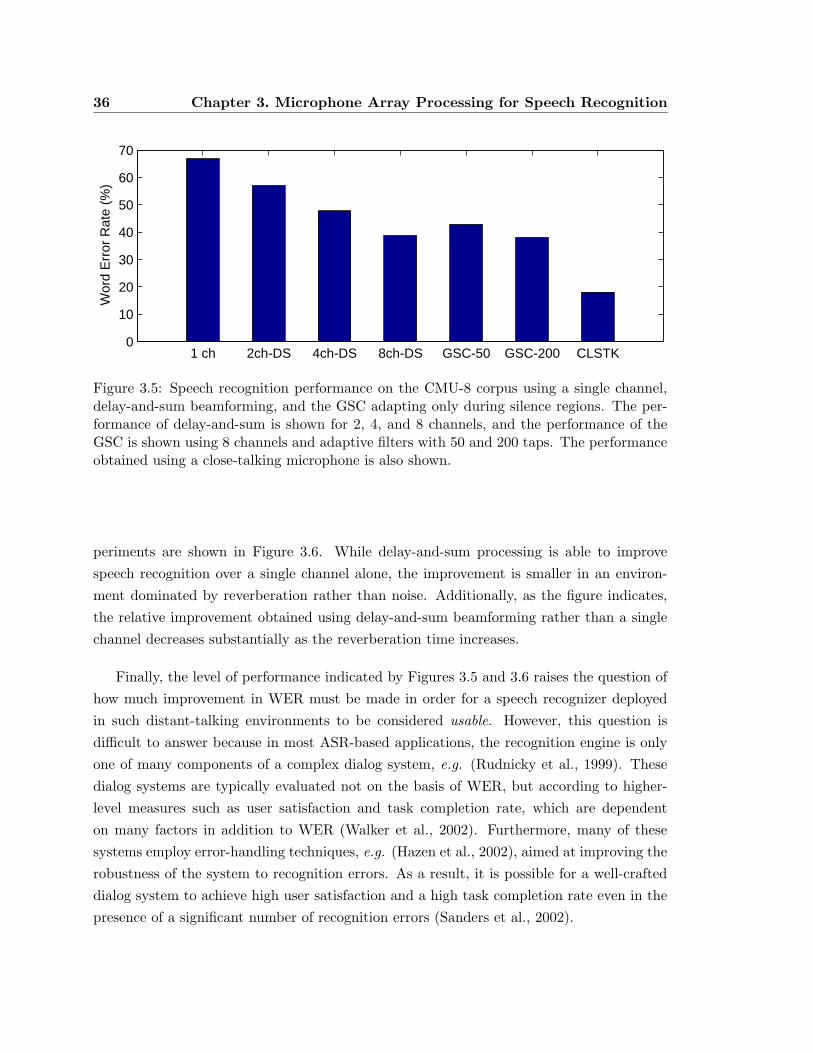
36 Chapter 3. Microphone Array Processing for Speech Recognition
1 ch 2ch-DS 4ch-DS 8ch-DS GSC-50 GSC-200 CLSTK0
10
20
30
40
50
60
70
Wor
d E
rror
Rat
e (%
)
Figure 3.5: Speech recognition performance on the CMU-8 corpus using a single channel,delay-and-sum beamforming, and the GSC adapting only during silence regions. The per-formance of delay-and-sum is shown for 2, 4, and 8 channels, and the performance of theGSC is shown using 8 channels and adaptive filters with 50 and 200 taps. The performanceobtained using a close-talking microphone is also shown.
periments are shown in Figure 3.6. While delay-and-sum processing is able to improve
speech recognition over a single channel alone, the improvement is smaller in an environ-
ment dominated by reverberation rather than noise. Additionally, as the figure indicates,
the relative improvement obtained using delay-and-sum beamforming rather than a single
channel decreases substantially as the reverberation time increases.
Finally, the level of performance indicated by Figures 3.5 and 3.6 raises the question of
how much improvement in WER must be made in order for a speech recognizer deployed
in such distant-talking environments to be considered usable. However, this question is
difficult to answer because in most ASR-based applications, the recognition engine is only
one of many components of a complex dialog system, e.g. (Rudnicky et al., 1999). These
dialog systems are typically evaluated not on the basis of WER, but according to higher-
level measures such as user satisfaction and task completion rate, which are dependent
on many factors in addition to WER (Walker et al., 2002). Furthermore, many of these
systems employ error-handling techniques, e.g. (Hazen et al., 2002), aimed at improving the
robustness of the system to recognition errors. As a result, it is possible for a well-crafted
dialog system to achieve high user satisfaction and a high task completion rate even in the
presence of a significant number of recognition errors (Sanders et al., 2002).
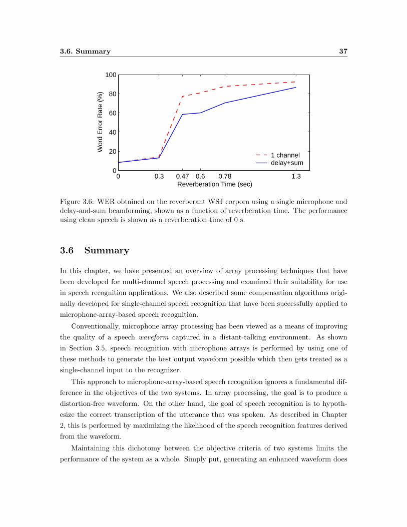
3.6. Summary 37
0 0.3 0.47 0.6 0.78 1.30
20
40
60
80
100
Wor
d E
rror
Rat
e (%
)
Reverberation Time (sec)
1 channeldelay+sum
Figure 3.6: WER obtained on the reverberant WSJ corpora using a single microphone anddelay-and-sum beamforming, shown as a function of reverberation time. The performanceusing clean speech is shown as a reverberation time of 0 s.
3.6 Summary
In this chapter, we have presented an overview of array processing techniques that have
been developed for multi-channel speech processing and examined their suitability for use
in speech recognition applications. We also described some compensation algorithms origi-
nally developed for single-channel speech recognition that have been successfully applied to
microphone-array-based speech recognition.
Conventionally, microphone array processing has been viewed as a means of improving
the quality of a speech waveform captured in a distant-talking environment. As shown
in Section 3.5, speech recognition with microphone arrays is performed by using one of
these methods to generate the best output waveform possible which then gets treated as a
single-channel input to the recognizer.
This approach to microphone-array-based speech recognition ignores a fundamental dif-
ference in the objectives of the two systems. In array processing, the goal is to produce a
distortion-free waveform. On the other hand, the goal of speech recognition is to hypoth-
esize the correct transcription of the utterance that was spoken. As described in Chapter
2, this is performed by maximizing the likelihood of the speech recognition features derived
from the waveform.
Maintaining this dichotomy between the objective criteria of two systems limits the
performance of the system as a whole. Simply put, generating an enhanced waveform does
38 Chapter 3. Microphone Array Processing for Speech Recognition
not necessarily improve recognition. The array processing scheme can only be expected
to improve recognition if it results in a sequence of features which maximizes, or at least
increases, the likelihood of the correct transcription.
We believe that this is why many array processing algorithms that are capable of gen-
erating significantly better output waveforms than simpler methods do not also produce
comparable gains in speech recognition accuracy. In the next chapter, we present a frame-
work for a new array processing methodology specifically designed for improved speech
recognition performance.
Chapter 4
Likelihood Maximizing
Beamforming
4.1 Introduction
Microphone array processing methods have historically been designed according to princi-
ples pertinent to signal enhancement applications. These algorithms are usually concerned
with generating the optimal output waveform and as such, they process the array signals
according to various signal-level criteria, e.g. minimizing signal error or maximizing SNR.
However, such criteria do not necessarily result in an improvement in the features subse-
quently derived for input to a speech recognition system. As a result, complicated array
processing schemes which are capable of producing high quality output signals may not re-
sult in significant improvements in speech recognition accuracy over much simpler methods,
such as delay-and-sum beamforming.
These methods approach the problem of microphone array processing for speech recogni-
tion as a signal processing problem. However, as described in Chapter 2, speech recognition
is not a signal processing problem but rather a pattern classification problem. Sound classes
are modeled by probability distribution functions. The speech waveform is converted into a
sequence of features vectors and the recognizer then compares these vectors to the statistical
class models. The output is a label corresponding to the sound class or sequence of sound
classes that has the maximum likelihood of generating the observed vectors. Therefore, in
order to improve speech recognition performance, the likelihood of the correct class must be
maximized, or at least increased relative to the other (incorrect) classes for a given input.
In order to do so, the following must be considered:
39
40 Chapter 4. Likelihood Maximizing Beamforming
1. the manner in which information is input to the recognition system, i.e. the featureextraction process
2. the manner in which these features are processed by the recognizer in order to generatea hypothesis
Thus, we recast the microphone array processing problem as one of finding the set of
array parameters which maximizes the likelihood of the correct hypothesis. In this chapter,
we present a solution to this problem in which these considerations are incorporated into
the framework of a filter-and-sum beamformer. We refer to this approach as LIkelihood
MAximizing BEAMforming (LIMABEAM). In this approach, information from the speech
recognition system itself will be used to find the array parameters that improve speech
recognition performance.
4.2 Filter-and-Sum Array Processing
In this work, we assume that filter-and-sum array processing can effectively compensate
for the distortion induced by additive noise and reverberation. In the filter-and-sum archi-
tecture, each microphone in the array has a corresponding filter. The signal captured by
each microphone is convolved with its corresponding filter and the filter outputs are then
summed together. Time-delay compensation may be applied prior to filtering, or may be
incorporated into the filters themselves, simply as a time-shift of the coefficients.
Assuming the filters have a finite impulse response (FIR), filter-and-sum processing is
expressed mathematically as
y[n] =
M−1∑
m=0
P−1∑
p=0
hm[p]xm[n− p− τm] (4.1)
where M is the number of microphones in the array, P is the length of the FIR filters, and
τm is the delay induced in the signal received by microphone m to align it to the other array
channels.
We define ξ to be the vector of all filter coefficients for all microphones, as
ξ = [h0[0], h0[1], . . . , hM−1[P − 2], hM−1[P − 1]]T (4.2)
Conventionally, filter parameters are chosen to optimize the beampattern, minimize
signal distortion, or suppress interfering signals, i.e. criteria that focus on the notion of a
desired signal. In contrast, because our goal is improved speech recognition performance, we
4.3. Likelihood Maximizing Beamforming (LIMABEAM) 41
consider the output waveform y[n] to be incidental and desire to find the filter parameters
that optimize recognition accuracy. Therefore, we forgo the notion of a desired signal, and
instead focus on a desired hypothesis.
4.3 Likelihood Maximizing Beamforming (LIMABEAM)
Speech recognition systems operate by finding the word string most likely to generate the
observed sequence of feature vectors, as measured by the statistical models of the recognition
system. In Chapter 2, we described how this can be performed according to Bayes optimal
classification as
w = argmaxw
P (Z|w)P (w) (4.3)
where Z = {z1, z2, . . . , zT } is the sequence of observed feature vectors,w = {w1, w2, . . . , wN}represents a possible word string and P (Z|w) and P (w) are the corresponding acoustic and
language scores, respectively.
When speech is captured by a microphone array, the feature vectors Z are a function of
both the incoming speech and the array processing parameters, ξ. By rewriting Equation
(4.3) to reflect the influence the array parameters have on recognition, we can see that in
microphone array scenarios, speech recognition is performed as
w = argmaxw
P (Z(ξ)|w)P (w) (4.4)
Our goal is to find the parameter vector ξ that will optimize recognition performance.
One logical approach to doing so is to choose the array parameters that maximize the like-
lihood of the correct transcription of the utterance that was spoken. This will increase the
difference between the likelihood score of the correct transcription and the scores of compet-
ing incorrect hypotheses, and thus, increase the probability that the correct transcription
will be hypothesized.
For the time being, let us assume that the correct transcription of the utterance, which
we notate as wC , is known. We can then maximize Equation (4.4) for the array parameters
ξ, as
ξ = argmaxξ
P (Z(ξ)|wC)P (wC) (4.5)
Because the transcription is assumed to be known a priori , P (wC) will not change
42 Chapter 4. Likelihood Maximizing Beamforming
regardless of the value of ξ and can be neglected. The maximum likelihood (ML) estimate
of the array parameters can now be defined as the vector that maximizes the acoustic
likelihood of the given sequence of words. This can be expressed as
ξ = argmaxξ
P (Z(ξ)|wC) (4.6)
In an HMM-based speech recognition system, the acoustic likelihood P (Z(ξ)|wC) is
computed as the total likelihood of all possible paths, i.e. state sequences, through HMMwC ,
the HMM for the sequence of words in the transcription wC . If SC represents the set of all
possible state sequences through HMMwC , and s represents one such state sequence, then
the maximum likelihood estimate of ξ can be written as
ξ = argmaxξ
∑
s∈SC
(∏
i
P (zi(ξ)|si)P (si|si−1,wC)
)(4.7)
While the maximum likelihood formulation is computed over all possible state sequences
for a given transcription, many of these sequences are highly unlikely. For computational
efficiency, we assume that the likelihood of a given transcription is largely represented by
the single most likely state sequence through HMMwC . Under this assumption, the ML
estimate of ξ becomes
ξ = argmaxξ,s∈SC
∏
i
P (zi(ξ)|si)P (si|si−1,wC) (4.8)
It will be more convenient and entirely equivalent to maximize the log likelihood rather
than the likelihood itself. Thus, Equation (4.8), becomes
ξ = argmaxξ,s∈SC
{∑
i
log(P (zi(ξ)|si) +∑
i
log(P (si|si−1,wC)
}(4.9)
According to Equation (4.9), in order to find ξ, the likelihood of the correct transcription
must be jointly optimized with respect to both the array parameters and the state sequence.
This joint optimization can be performed by alternately optimizing the state sequence and
the array processing parameters in an iterative manner, i.e. fixing the array parameters and
finding the optimal state sequence, then fixing the state sequence and finding the optimal
array parameters, and so on. This approach corresponds to alternately optimizing the left
and right summation terms in Equation (4.9).
In the following sections, we describe how to optimize the state sequence and the array

4.4. Optimizing the State Sequence 43
parameters.
4.4 Optimizing the State Sequence
Given set of array parameters ξ, the speech can be processed by the array and a sequence
of feature vectors Z(ξ) produced. Using the features vectors and the transcription wC , we
want to find the state sequence s = {s1, s2, . . . , sT } such that
s = argmaxs∈SC
∑
i
log(P (si|si−1,wC ,Z(ξ)) (4.10)
This state sequence s can be determined using the Viterbi algorithm (Viterbi, 1967). This
procedure is known as forced alignment or Viterbi alignment. In forced alignment, the
sentence HMM corresponding to the given transcription is assembled and then the alignment
between the states of the HMM and the given sequence of feature vectors that results in
the maximum overall likelihood is found using dynamic programming. This is done in
an efficient, recursive manner by exploiting the fact that the underlying random process
modeled by the HMM (in this case, speech), is assumed to be Markov. More details about
forced alignment can be found in (Rabiner & Juang, 1993; Jelinek, 1997).
4.5 Optimizing the Array Parameters
We now turn to the question of how to find the array parameters which maximize the
likelihood of a given state sequence, s. That is, we are interested in finding ξ such that
ξ = argmaxξ
∑
i
log(P (zi(ξ)|si) (4.11)
This acoustic likelihood expression cannot be directly maximized with respect to the
array parameters ξ for two reasons. First, the state distributions used in most HMM-based
speech recognition systems are complicated density functions, i.e mixtures of Gaussians.
Second, the acoustic likelihood of an utterance and the parameter vector ξ are related
through a series of linear and non-linear mathematical operations performed to convert a
waveform into a sequence of feature vectors, as discussed in Section 2.2.1. Therefore, for a
given HMM state sequence, no closed-form solution for the optimal value of ξ exists. As a
result, non-linear optimization methods must be used.
We will employ a gradient-based approach to finding the optimal value of ξ. For con-
venience, we define L(ξ) to be the total log likelihood of the observation vectors given an
44 Chapter 4. Likelihood Maximizing Beamforming
HMM state sequence. Thus,
L(ξ) =∑
i
log(P (zi(ξ)|si) (4.12)
Thus, we need to compute the gradient of L(ξ) with respect to the array parameters ξ.
Using the definition of ξ given by Equation (4.2), we define the gradient vector ∇ξL(ξ) as
∇ξL(ξ) =
[∂L(ξ)
∂h0[0],∂L(ξ)
∂h0[1], . . . ,
∂L(ξ)
∂hM−1[P − 1]
]T(4.13)
Clearly, the computation of gradient vector is dependent on the form of the state dis-
tributions used by the recognition system and the features used for recognition. In the
following sections, we derive the gradient expressions when the state distributions are mod-
eled as Gaussian distributions or mixtures of Gaussians. In both cases, the features are
assumed to be mel frequency cepstral coefficients or log mel spectra.
4.5.1 Gaussian State Output Distributions
We now derive the expression for∇ξL(ξ) for the case where the HMM state distributions are
multivariate Gaussian distributions with diagonal covariance matrices. This is the simplest
density function commonly used by HMM-based recognition systems. If we define µi and
Σi to be the mean vector and covariance matrix, respectively, of the pdf of the most likely
HMM state at frame i, the total log likelihood for an utterance can be expressed as
L(ξ) =∑
i
−1
2(zi(ξ)− µi)T Σ−1
i (zi(ξ)− µi) + κi (4.14)
where κi is a normalizing constant. We are interested in computed the gradient of L(ξ)
with respect to ξ. Using the chain rule, this is expressed as
∇ξL(ξ) = −∑
i
∂zi(ξ)
∂ξΣ−1i (zi(ξ)− µi) (4.15)
where ∂zi(ξ)/∂ξ is the Jacobian matrix, composed of the partial derivatives of each element
of the feature vector with respect to each of array parameters. The Jacobian is of dimension
MP × L where M is the number of microphones, P is the number of parameters per
microphone, and L is the dimension of the feature vector. The full derivation of the Jacobian
matrix when the array parameters are FIR filter coefficients and the feature vectors are mel
frequency cepstra or log mel spectra is given in Appendix A.

4.5. Optimizing the Array Parameters 45
4.5.2 Mixture of Gaussians State Output Distributions
Most state-of-the-art recognizers do not model the state output distributions as single Gaus-
sians but rather as mixtures of Gaussians. We now develop the gradient expression for this
case. The log likelihood that a feature vector at frame i was generated by HMM state si,
modeled as a mixture of K Gaussians, can be expressed as
log(P (zi(ξ)|si)) = log
{K∑
k=1
αikκik exp
(−1
2(zi(ξ)− µik)T Σ−1
ik (zi(ξ)− µik))}
(4.16)
= log
{K∑
k=1
exp
(−1
2(zi(ξ)− µik)T Σ−1
ik (zi(ξ)− µik) + log(αikκik)
)}
(4.17)
where αik is the mixture weight of the kth Gaussian in state si and κik is a normalizing
constant as before.
For convenience, we represent the term inside the exp() operator in Equation (4.17) as
Gik(ξ). The total log likelihood of a given state sequence whose output distributions are
modeled as mixtures of Gaussians can then be expressed compactly as
L(ξ) =∑
i
log
(K∑
k=1
exp (Gik(ξ))
)(4.18)
As before, the gradient of Equation (4.18) is computed using the chain rule, giving
∇ξL(ξ) =∑
i
{1
∑Kj=1 exp (Gij(ξ))
K∑
k=1
exp (Gik(ξ))∂Gik(ξ)
∂ξ
}(4.19)
where we have introduced the summation index j for clarity. This can be rewritten as
∇ξL(ξ) =∑
i
K∑
k=1
(exp (Gik(ξ))
∑Kj=1 exp (Gij(ξ))
)∂Gik(ξ)
∂ξ(4.20)
The term in the parenthesis represents the a posteriori probability of the kth mixture
component, which we represent as γik(ξ) to reflect its dependence on the array parameters
ξ. We can therefore compactly rewrite Equation (4.20) as
∇ξL(ξ) =∑
i
K∑
k=1
γik(ξ)∂Gik(ξ)
∂ξ(4.21)
46 Chapter 4. Likelihood Maximizing Beamforming
Using Equation (4.15), the expression for the gradient of Gik(ξ) can be expressed as
∂Gik(ξ)
∂ξ= −∂zi(ξ)
∂ξΣ−1ik (zi(ξ)− µik) (4.22)
where ∂zi(ξ)/∂ξ is the Jacobian matrix, as before.
Thus, the complete gradient expression when the HMM state distributions are modeled
as mixtures of Gaussians is
∇ξL(ξ) = −∑
i
K∑
k=1
γik(ξ)∂zi(ξ)
∂ξΣ−1ik (zi(ξ)− µik) (4.23)
Comparing Equations (4.15) and (4.23), the gradient expresssion in the Gaussian mix-
ture case is simply a weighted sum of the gradients of each of the Gaussian components
in the mixture, where the weight on each mixture component represents its a posteriori
probability of generating the observed feature vector.
4.5.3 Gradient-based Array Parameter Optimization
Using the gradient vector defined in either Equation (4.15) or Equation (4.23), the array
parameters can be optimized using hill-climbing techniques, such as conventional gradient
descent (Haykin, 2002). However, improved convergence performance can be achieved by
methods which utilize second-order derivative information, i.e. the Hessian, estimated
from first-order gradients. In this work, we perform optimization using the method of
conjugate gradients. More information about conjugate gradient optimization can be found
in (Nocedal & Wright, 1999).
4.6 Evaluating LIMABEAM Using Oracle State Sequences
To test the proposed gradient-based array parameter optimization scheme, experiments were
performed in which the filter parameters were optimized using state sequences generated
from a priori knowledge of the utterance transcriptions and features derived from close-
talking microphone recordings. Because these state sequences were derived from information
normally not available, we refer to them as oracle state sequences. By using oracle state
sequences, the upper bound on the performance of the proposed LIMABEAM algorithm
can be studied.
Array parameter optimization was performed in the log mel spectral domain. This was
done for two reasons. First, because the log mel spectra are derived from the energy in a
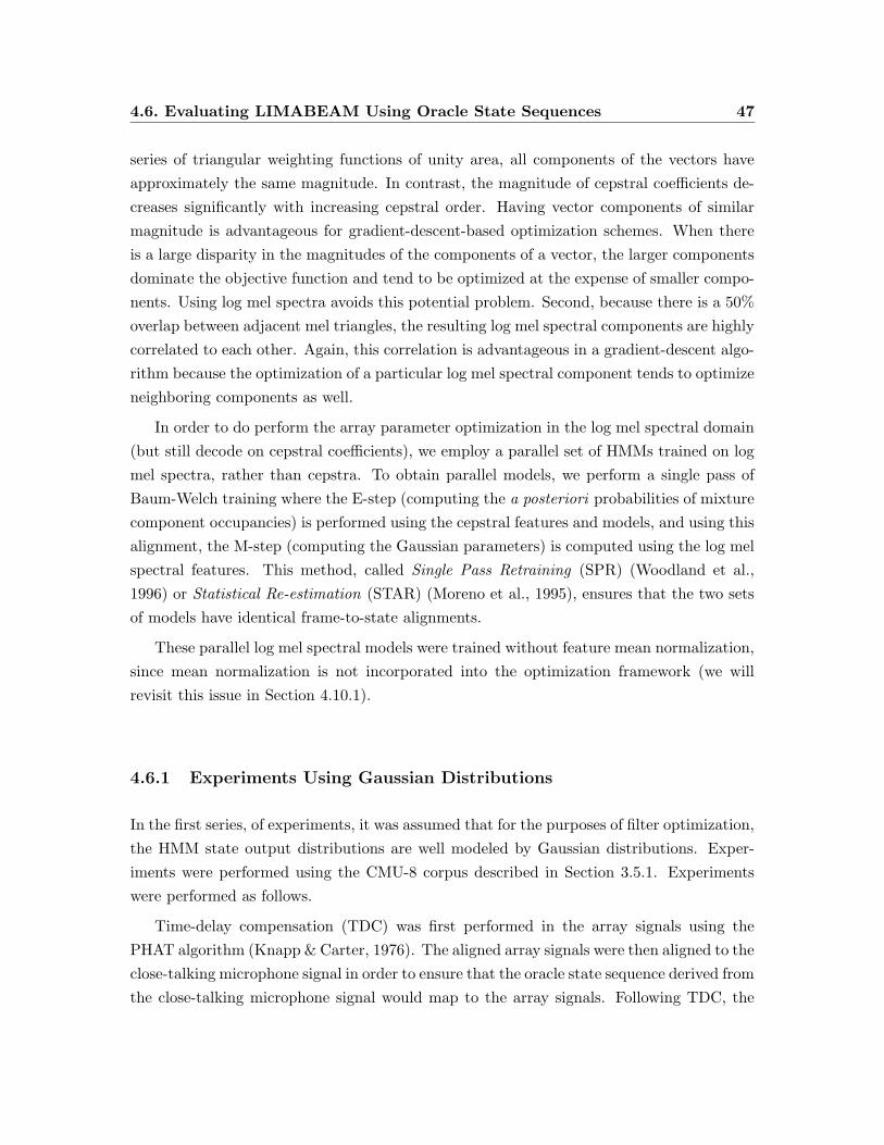
4.6. Evaluating LIMABEAM Using Oracle State Sequences 47
series of triangular weighting functions of unity area, all components of the vectors have
approximately the same magnitude. In contrast, the magnitude of cepstral coefficients de-
creases significantly with increasing cepstral order. Having vector components of similar
magnitude is advantageous for gradient-descent-based optimization schemes. When there
is a large disparity in the magnitudes of the components of a vector, the larger components
dominate the objective function and tend to be optimized at the expense of smaller compo-
nents. Using log mel spectra avoids this potential problem. Second, because there is a 50%
overlap between adjacent mel triangles, the resulting log mel spectral components are highly
correlated to each other. Again, this correlation is advantageous in a gradient-descent algo-
rithm because the optimization of a particular log mel spectral component tends to optimize
neighboring components as well.
In order to do perform the array parameter optimization in the log mel spectral domain
(but still decode on cepstral coefficients), we employ a parallel set of HMMs trained on log
mel spectra, rather than cepstra. To obtain parallel models, we perform a single pass of
Baum-Welch training where the E-step (computing the a posteriori probabilities of mixture
component occupancies) is performed using the cepstral features and models, and using this
alignment, the M-step (computing the Gaussian parameters) is computed using the log mel
spectral features. This method, called Single Pass Retraining (SPR) (Woodland et al.,
1996) or Statistical Re-estimation (STAR) (Moreno et al., 1995), ensures that the two sets
of models have identical frame-to-state alignments.
These parallel log mel spectral models were trained without feature mean normalization,
since mean normalization is not incorporated into the optimization framework (we will
revisit this issue in Section 4.10.1).
4.6.1 Experiments Using Gaussian Distributions
In the first series, of experiments, it was assumed that for the purposes of filter optimization,
the HMM state output distributions are well modeled by Gaussian distributions. Exper-
iments were performed using the CMU-8 corpus described in Section 3.5.1. Experiments
were performed as follows.
Time-delay compensation (TDC) was first performed in the array signals using the
PHAT algorithm (Knapp & Carter, 1976). The aligned array signals were then aligned to the
close-talking microphone signal in order to ensure that the oracle state sequence derived from
the close-talking microphone signal would map to the array signals. Following TDC, the
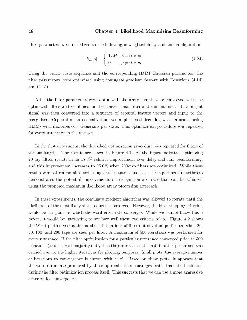
48 Chapter 4. Likelihood Maximizing Beamforming
filter parameters were initialized to the following unweighted delay-and-sum configuration:
hm[p] =
{1/M p = 0, ∀ m0 p 6= 0, ∀ m
(4.24)
Using the oracle state sequence and the corresponding HMM Gaussian parameters, the
filter parameters were optimized using conjugate gradient descent with Equations (4.14)
and (4.15).
After the filter parameters were optimized, the array signals were convolved with the
optimized filters and combined in the conventional filter-and-sum manner. The output
signal was then converted into a sequence of cepstral feature vectors and input to the
recognizer. Cepstral mean normalization was applied and decoding was performed using
HMMs with mixtures of 8 Gaussians per state. This optimization procedure was repeated
for every utterance in the test set.
In the first experiment, the described optimization procedure was repeated for filters of
various lengths. The results are shown in Figure 4.1. As the figure indicates, optimizing
20-tap filters results in an 18.3% relative improvement over delay-and-sum beamforming,
and this improvement increases to 25.0% when 200-tap filters are optimized. While these
results were of course obtained using oracle state sequences, the experiment nonetheless
demonstrates the potential improvements on recognition accuracy that can be achieved
using the proposed maximum likelihood array processing approach.
In these experiments, the conjugate gradient algorithm was allowed to iterate until the
likelihood of the most likely state sequence converged. However, the ideal stopping criterion
would be the point at which the word error rate converges. While we cannot know this a
priori , it would be interesting to see how well these two criteria relate. Figure 4.2 shows
the WER plotted versus the number of iterations of filter optimization performed when 20,
50, 100, and 200 taps are used per filter. A maximum of 500 iterations was performed for
every utterance. If the filter optimization for a particular utterance converged prior to 500
iterations (and the vast majority did), then the error rate at the last iteration performed was
carried over to the higher iterations for plotting purposes. In all plots, the average number
of iterations to convergence is shown with a ‘◦’. Based on these plots, it appears that
the word error rate produced by these optimal filters converges faster than the likelihood
during the filter optimization process itself. This suggests that we can use a more aggressive
criterion for convergence.
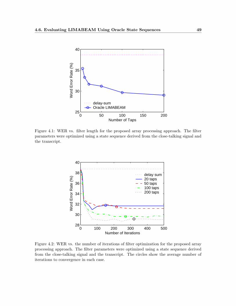
4.6. Evaluating LIMABEAM Using Oracle State Sequences 49
0 50 100 150 20025
30
35
40
Number of Taps
Wor
d E
rror
Rat
e (%
)
delay-sumOracle LIMABEAM
Figure 4.1: WER vs. filter length for the proposed array processing approach. The filterparameters were optimized using a state sequence derived from the close-talking signal andthe transcript.
0 100 200 300 400 50028
30
32
34
36
38
40
Number of Iterations
Wor
d E
rror
Rat
e (%
) delay sum20 taps50 taps100 taps200 taps
Figure 4.2: WER vs. the number of iterations of filter optimization for the proposed arrayprocessing approach. The filter parameters were optimized using a state sequence derivedfrom the close-talking signal and the transcript. The circles show the average number ofiterations to convergence in each case.
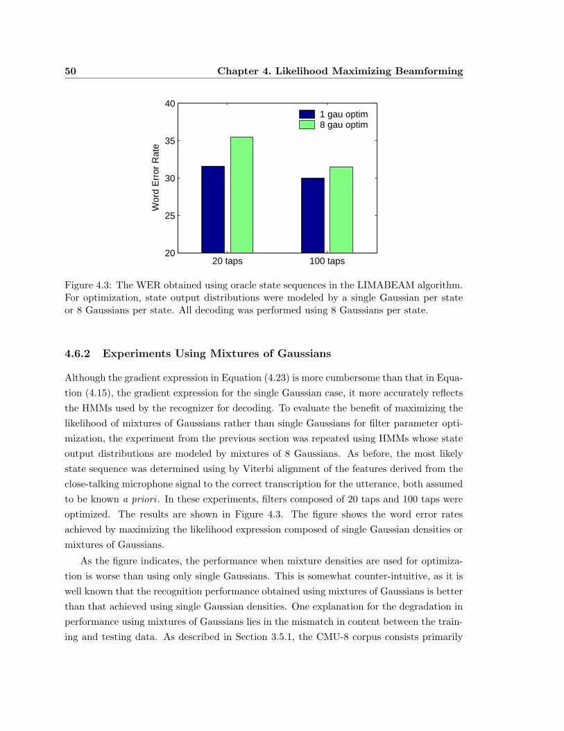
50 Chapter 4. Likelihood Maximizing Beamforming
20 taps 100 taps20
25
30
35
40
Wor
d E
rror
Rat
e
1 gau optim8 gau optim
Figure 4.3: The WER obtained using oracle state sequences in the LIMABEAM algorithm.For optimization, state output distributions were modeled by a single Gaussian per stateor 8 Gaussians per state. All decoding was performed using 8 Gaussians per state.
4.6.2 Experiments Using Mixtures of Gaussians
Although the gradient expression in Equation (4.23) is more cumbersome than that in Equa-
tion (4.15), the gradient expression for the single Gaussian case, it more accurately reflects
the HMMs used by the recognizer for decoding. To evaluate the benefit of maximizing the
likelihood of mixtures of Gaussians rather than single Gaussians for filter parameter opti-
mization, the experiment from the previous section was repeated using HMMs whose state
output distributions are modeled by mixtures of 8 Gaussians. As before, the most likely
state sequence was determined using by Viterbi alignment of the features derived from the
close-talking microphone signal to the correct transcription for the utterance, both assumed
to be known a priori . In these experiments, filters composed of 20 taps and 100 taps were
optimized. The results are shown in Figure 4.3. The figure shows the word error rates
achieved by maximizing the likelihood expression composed of single Gaussian densities or
mixtures of Gaussians.
As the figure indicates, the performance when mixture densities are used for optimiza-
tion is worse than using only single Gaussians. This is somewhat counter-intuitive, as it is
well known that the recognition performance obtained using mixtures of Gaussians is better
than that achieved using single Gaussian densities. One explanation for the degradation in
performance using mixtures of Gaussians lies in the mismatch in content between the train-
ing and testing data. As described in Section 3.5.1, the CMU-8 corpus consists primarily
4.7. The Calibrated LIMABEAM Algorithm 51
strings of connected digits and letters along with some additional keywords. Unfortunately,
no training corpus large enough data to train context-dependent continuous density HMMs
was available for such a task. As a result, the HMMs were trained using the WSJ corpus,
a large vocabulary task consisting of continuous read speech. Thus, there is somewhat of a
mismatch in the tasks of the training and test sets, which inhibits the performance when
mixtures of Gaussians are used for filter optimization.
4.6.3 Summary of Results Using Oracle LIMABEAM
In this section, we have shown that the proposed Likelihood Maximizing Beamforming
(LIMABEAM) approach is capable of achieving significant improvements over a conven-
tional delay-and-sum beamformer provided that the most likely state sequence for the cor-
rect transcription of the utterance is known a priori . Such improvements are possible even
when the filter lengths are small, e.g. 20 taps. This compares favorably to the recognition
performance of the Generalized Sidelobe Canceller, as was shown in Figure 3.5. Using the
GSC, the WER with 50-tap filters was worse than that of delay-and-sum, and the WER
with 200-tap filters was only marginally better. Using the ML array processing approach
described here, 200-tap filters resulted in a 25% relative improvement over delay-and-sum.
We also saw that for filter optimization, modeling the HMM state output distributions
as mixtures of Gaussians resulted in worse recognition accuracy on the CMU-8 corpus than
single Gaussians. We believe this is due in large part to the mismatch in task between the
training and testing corpora. Optimization with mixtures of Gaussians will be revisited in
Chapters 5 and 6. However, for the remainder of the experiments in this chapter, we will
use single Gaussian distributions for optimization.
Of course, all the improvements in recognition accuracy were achieved using oracle
state sequences generated from the transcriptions of the utterances and the close-talking
microphone signal, both assumed to be known a priori . Of course, in a realistic scenario,
this information is not available. In the following sections, LIMABEAM-based algorithms
that do not require oracle information will be presented.
4.7 The Calibrated LIMABEAM Algorithm
In Section 4.3, an approach to array processing was presented in which the array processor
combined the received signals in such a manner so as to maximize the likelihood that the
recognition system would estimate the correct hypothesis. This was achieved by choosing
array parameters (in this case, a set of filter coefficients) which generate a sequence of
52 Chapter 4. Likelihood Maximizing Beamforming
feature vectors for which the likelihood of the correct transcription is maximum. This
approach resulted in significantly improved recognition performance over a conventional
delay-and-sum beamformer. However, the proposed algorithm required a priori knowledge
of the utterance transcription in order to generate the optimal state sequence. Clearly, we
are faced with a paradox: prior knowledge of the correct transcription is required in order
to maximize its likelihood. Yet, if we had such knowledge, there would be no need for
recognition in the first place.
In this section, we present one solution to this paradox. The LIMABEAM algorithm
is cast as a method of microphone array calibration. The array parameters are optimized
using an utterance with a known transcription spoken by the user. After optimization,
these parameters are fixed for future processing. Because the optimization is performed
using a known transcription, we refer to this as supervised optimization. We now describe
the calibration algorithm in more detail.
In the calibration scenario, the user is asked to speak an enrollment utterance with a
known transcription. As before, an estimate of the most likely state sequence corresponding
to the enrollment transcription is made using the Viterbi algorithm. However, because the
close-talking microphone signal is no longer available, the features used to estimate the
state sequence are derived directly from the array signals themselves. These features can be
generated using an initial set of filters, e.g. from a previous calibration session or a simple
delay-and-sum configuration.
Using this estimated state sequence, the filter parameters are optimized as before. This
constitutes one iteration of calibration. Of course, this is not to be confused with the number
of iterations of conjugate gradient descent in the filter optimization process, which is run
to convergence unless otherwise noted. Using the optimized filter parameters, a second
iteration of calibration can be performed. An improved set of features for the calibration
utterance is generated and used to re-estimate the state sequence. The filter optimization
process can then be repeated using the updated state sequence. The calibration process
continues in an iterative manner until the overall likelihood converges. Once convergence
occurs, the calibration process is complete. The resulting filters are now used to process
future incoming speech to the array. Because we are calibrating the array parameters to
maximize the likelihood of the enrollment utterance, we refer to this method as Calibrated
LIMABEAM. A flowchart of the calibration algorithm is shown in Figure 4.4.
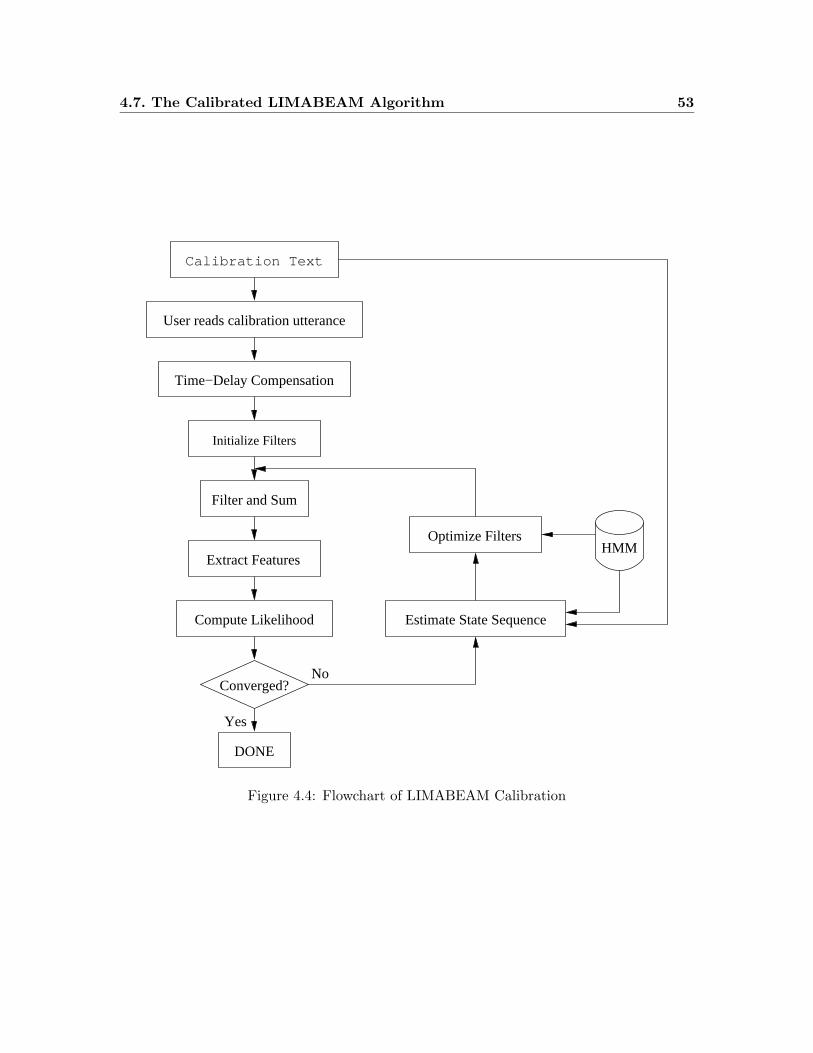
4.7. The Calibrated LIMABEAM Algorithm 53
User reads calibration utterance
Time−Delay Compensation
Initialize Filters
Filter and Sum
Extract Features
Compute Likelihood
Converged?
DONE
Estimate State Sequence
HMMOptimize Filters
Yes
No
Calibration Text
Figure 4.4: Flowchart of LIMABEAM Calibration
54 Chapter 4. Likelihood Maximizing Beamforming
4.7.1 Experimental Results Using Calibrated LIMABEAM
Experiments were performed to test the proposed array calibration procedure. In the first se-
ries of experiments, a single utterance from each speaker was used for calibration. An utter-
ance common to all speakers was chosen as the calibration utterance (P-I-T-T-S-B-U-R-G-H).
For each speaker, the filters were initialized to the delay-and-sum configuration in Equation
(4.24). The array signals of the calibration utterance were processed and recognition fea-
tures generated from the delay-and-sum output signal. Using these features and the known
utterance transcription, the most likely state sequence was estimated via forced alignment.
The filter parameters were then optimized to maximize the likelihood of this state sequence.
As before, the filter parameter optimization was performed in the log mel spectral domain
and the likelihood expression for the calibration utterance was formed from single Gaus-
sian HMM state distributions. In these experiments, calibration was terminated after one
full iteration. After calibration was complete, the optimized filters were fixed and used to
process the remaining utterances for that speaker.
Figure 4.5 shows the WER obtained using Calibrated LIMABEAM as a function of filter
length. Also shown in the figure are the results from the oracle experiment performed in
Section 4.6.1, in which the filter parameters were optimized for each utterance individually
using a priori knowledge of the transcription and close-talking microphone signal. As the
figure indicates, the calibration algorithm tracks the oracle experiment quite closely until
filters with more than 20 taps are used. At that point, the performance becomes increasingly
worse than the oracle case as the number of filter parameters increases. As the number of
taps per filter approaches 200, the calibration algorithm performs worse than delay-and-sum
beamforming.
The degradation in performance obtained when the filter length exceeds 20 taps is likely
caused by overfitting of the filters to the calibration utterance. Because we are attempting
to obtain filters that generalize to future utterances using a very small amount of data
(only a single utterance), the chances of overfitting are quite high. As a result, the number
of parameters to optimize needs to be limited in order to obtain performance that will
generalize to unseen utterances.
We expect that as the amount of data used for calibration increases, the number of
parameters that can be reliably estimated will also increase. To test this hypothesis, the
calibration experiment previously described was repeated. However, in this case, calibra-
tion was performed using three utterances concatenated together, rather than just a single
utterance. The results are shown in Table 4.1 for calibration of filters with 20 and 50 taps.
Note that the word error rates obtained using conventional delay-and-sum processing and

4.7. The Calibrated LIMABEAM Algorithm 55
0 50 100 150 20025
30
35
40
45
Number of Taps
Wor
d E
rror
Rat
e (%
)
delay-sumCalib LIMABEAMOracle LIMABEAM
Figure 4.5: WER vs. filter length obtained using the Calibrated LIMABEAM algorithm.The solid line shows performance obtained when the array parameters are optimized usingoracle state sequences while the dashed line shows performance for the array calibrationapproach when the filter parameters are optimized using only a single utterance with knowntranscription. The performance obtained using conventional delay-and-sum processing isshown for reference.
using array calibration based on a single utterance are slightly different from those obtained
in the previous experiment. This change arises because we are performing recognition with
fewer utterances, since two of the utterances for each speaker previously in the test set are
now used for calibration, and hence not scored in decoding.
As the results in the table show, the calibration algorithm has approximately the same
performance when 20-tap filters are calibrated using a single utterance or three concate-
nated utterances. However, the performance obtained when 50-tap filters are calibrated
dramatically improves when more calibration data is used. As expected, we achieve better
performance using more filter parameters, provided there is enough calibration data to re-
liably estimate filters that generalize well to unseen test data. Furthermore, with increased
calibration data, the WER achieved by the calibration algorithm using 50 taps per filter is
very close to that of the oracle case with the same number of parameters.
Finally, an experiment was performed to determine if additional improvement could
be obtained from additional calibration iterations. The experiment was performed on the
longer, concatenated calibration utterances described in the previous experiment, with 50-
tap filters. After the initial pass of calibration was complete, a new set of features was
derived from the calibration utterance by processing the array signals through the optimized
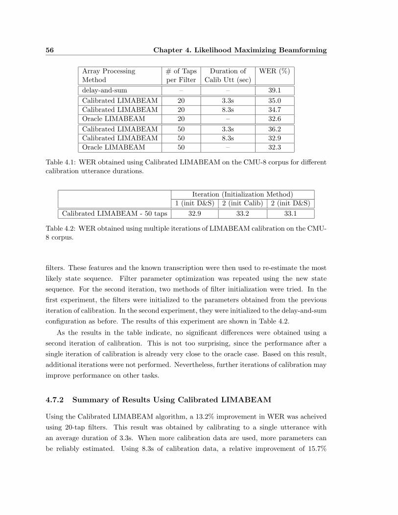
56 Chapter 4. Likelihood Maximizing Beamforming
Array Processing # of Taps Duration of WER (%)Method per Filter Calib Utt (sec)
delay-and-sum – – 39.1
Calibrated LIMABEAM 20 3.3s 35.0
Calibrated LIMABEAM 20 8.3s 34.7
Oracle LIMABEAM 20 – 32.6
Calibrated LIMABEAM 50 3.3s 36.2
Calibrated LIMABEAM 50 8.3s 32.9
Oracle LIMABEAM 50 – 32.3
Table 4.1: WER obtained using Calibrated LIMABEAM on the CMU-8 corpus for differentcalibration utterance durations.
Iteration (Initialization Method)1 (init D&S) 2 (init Calib) 2 (init D&S)
Calibrated LIMABEAM - 50 taps 32.9 33.2 33.1
Table 4.2: WER obtained using multiple iterations of LIMABEAM calibration on the CMU-8 corpus.
filters. These features and the known transcription were then used to re-estimate the most
likely state sequence. Filter parameter optimization was repeated using the new state
sequence. For the second iteration, two methods of filter initialization were tried. In the
first experiment, the filters were initialized to the parameters obtained from the previous
iteration of calibration. In the second experiment, they were initialized to the delay-and-sum
configuration as before. The results of this experiment are shown in Table 4.2.
As the results in the table indicate, no significant differences were obtained using a
second iteration of calibration. This is not too surprising, since the performance after a
single iteration of calibration is already very close to the oracle case. Based on this result,
additional iterations were not performed. Nevertheless, further iterations of calibration may
improve performance on other tasks.
4.7.2 Summary of Results Using Calibrated LIMABEAM
Using the Calibrated LIMABEAM algorithm, a 13.2% improvement in WER was acheived
using 20-tap filters. This result was obtained by calibrating to a single utterance with
an average duration of 3.3s. When more calibration data are used, more parameters can
be reliably estimated. Using 8.3s of calibration data, a relative improvement of 15.7%
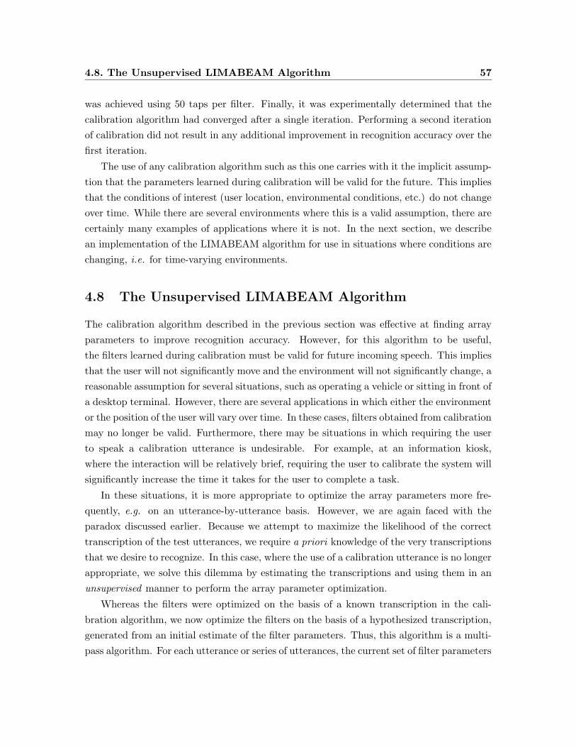
4.8. The Unsupervised LIMABEAM Algorithm 57
was achieved using 50 taps per filter. Finally, it was experimentally determined that the
calibration algorithm had converged after a single iteration. Performing a second iteration
of calibration did not result in any additional improvement in recognition accuracy over the
first iteration.
The use of any calibration algorithm such as this one carries with it the implicit assump-
tion that the parameters learned during calibration will be valid for the future. This implies
that the conditions of interest (user location, environmental conditions, etc.) do not change
over time. While there are several environments where this is a valid assumption, there are
certainly many examples of applications where it is not. In the next section, we describe
an implementation of the LIMABEAM algorithm for use in situations where conditions are
changing, i.e. for time-varying environments.
4.8 The Unsupervised LIMABEAM Algorithm
The calibration algorithm described in the previous section was effective at finding array
parameters to improve recognition accuracy. However, for this algorithm to be useful,
the filters learned during calibration must be valid for future incoming speech. This implies
that the user will not significantly move and the environment will not significantly change, a
reasonable assumption for several situations, such as operating a vehicle or sitting in front of
a desktop terminal. However, there are several applications in which either the environment
or the position of the user will vary over time. In these cases, filters obtained from calibration
may no longer be valid. Furthermore, there may be situations in which requiring the user
to speak a calibration utterance is undesirable. For example, at an information kiosk,
where the interaction will be relatively brief, requiring the user to calibrate the system will
significantly increase the time it takes for the user to complete a task.
In these situations, it is more appropriate to optimize the array parameters more fre-
quently, e.g. on an utterance-by-utterance basis. However, we are again faced with the
paradox discussed earlier. Because we attempt to maximize the likelihood of the correct
transcription of the test utterances, we require a priori knowledge of the very transcriptions
that we desire to recognize. In this case, where the use of a calibration utterance is no longer
appropriate, we solve this dilemma by estimating the transcriptions and using them in an
unsupervised manner to perform the array parameter optimization.
Whereas the filters were optimized on the basis of a known transcription in the cali-
bration algorithm, we now optimize the filters on the basis of a hypothesized transcription,
generated from an initial estimate of the filter parameters. Thus, this algorithm is a multi-
pass algorithm. For each utterance or series of utterances, the current set of filter parameters
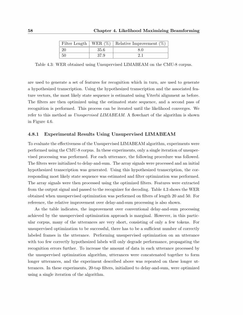
58 Chapter 4. Likelihood Maximizing Beamforming
Filter Length WER (%) Relative Improvement (%)
20 35.6 8.0
50 37.9 2.1
Table 4.3: WER obtained using Unsupervised LIMABEAM on the CMU-8 corpus.
are used to generate a set of features for recognition which in turn, are used to generate
a hypothesized transcription. Using the hypothesized transcription and the associated fea-
ture vectors, the most likely state sequence is estimated using Viterbi alignment as before.
The filters are then optimized using the estimated state sequence, and a second pass of
recognition is performed. This process can be iterated until the likelihood converges. We
refer to this method as Unsupervised LIMABEAM. A flowchart of the algorithm is shown
in Figure 4.6.
4.8.1 Experimental Results Using Unsupervised LIMABEAM
To evaluate the effectiveness of the Unsupervised LIMABEAM algorithm, experiments were
performed using the CMU-8 corpus. In these experiments, only a single iteration of unsuper-
vised processing was performed. For each utterance, the following procedure was followed.
The filters were initialized to delay-and-sum. The array signals were processed and an initial
hypothesized transcription was generated. Using this hypothesized transcription, the cor-
responding most likely state sequence was estimated and filter optimization was performed.
The array signals were then processed using the optimized filters. Features were extracted
from the output signal and passed to the recognizer for decoding. Table 4.3 shows the WER
obtained when unsupervised optimization was performed on filters of length 20 and 50. For
reference, the relative improvement over delay-and-sum processing is also shown.
As the table indicates, the improvement over conventional delay-and-sum processing
achieved by the unsupervised optimization approach is marginal. However, in this partic-
ular corpus, many of the utterances are very short, consisting of only a few tokens. For
unsupervised optimization to be successful, there has to be a sufficient number of correctly
labeled frames in the utterance. Performing unsupervised optimization on an utterance
with too few correctly hypothesized labels will only degrade performance, propagating the
recognition errors further. To increase the amount of data in each utterance processed by
the unsupervised optimization algorithm, utterances were concatenated together to form
longer utterances, and the experiment described above was repeated on these longer ut-
terances. In these experiments, 20-tap filters, initialized to delay-and-sum, were optimized
using a single iteration of the algorithm.
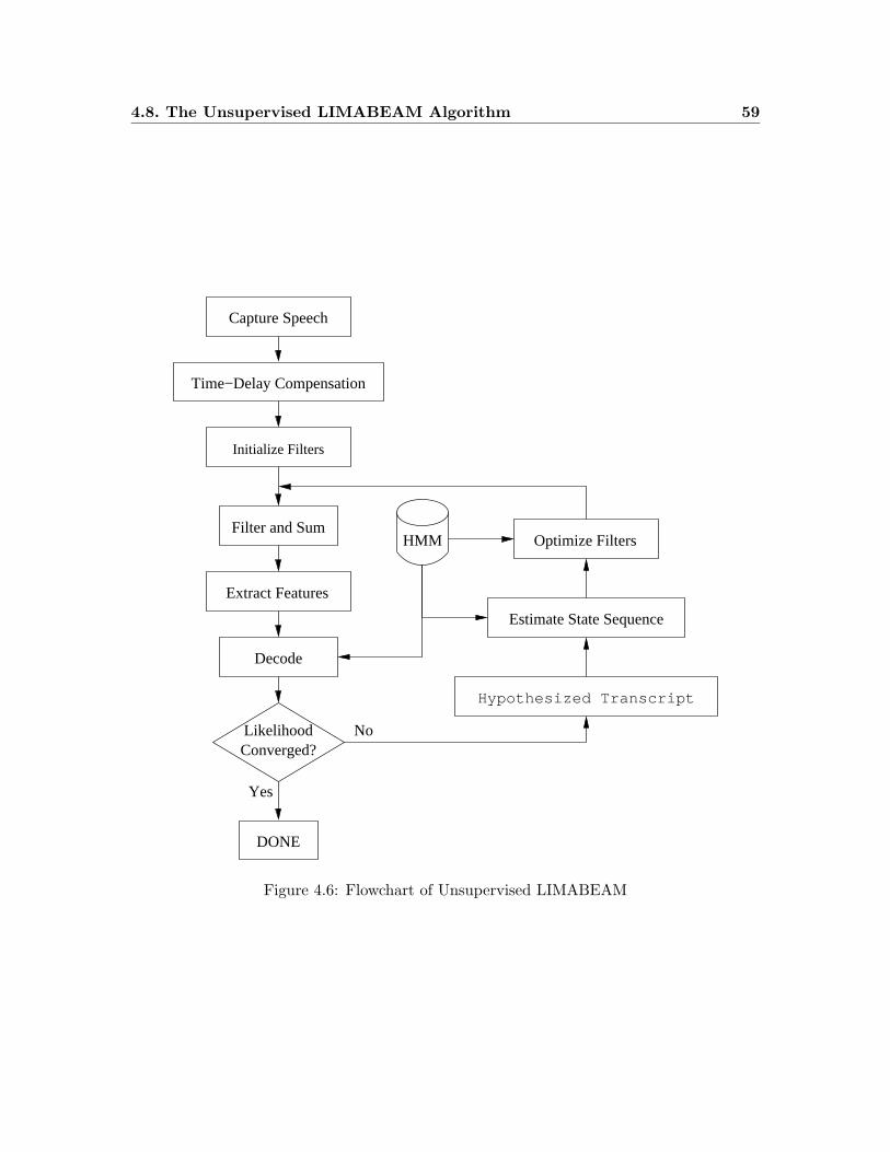
4.8. The Unsupervised LIMABEAM Algorithm 59
Time−Delay Compensation
Initialize Filters
LikelihoodConverged?
DONE
Filter and Sum
Extract Features
HMM Optimize Filters
Hypothesized Transcript
No
Yes
Capture Speech
Estimate State Sequence
Decode
Figure 4.6: Flowchart of Unsupervised LIMABEAM
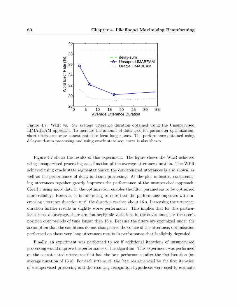
60 Chapter 4. Likelihood Maximizing Beamforming
0 5 10 15 20 25 30 3528
30
32
34
36
38
40
Average Utterance Duration
Wor
d E
rror
Rat
e (%
) delay-sumUnsuper LIMABEAMOracle LIMABEAM
Figure 4.7: WER vs. the average utterance duration obtained using the UnsupervisedLIMABEAM approach. To increase the amount of data used for parameter optimization,short utterances were concatenated to form longer ones. The performance obtained usingdelay-and-sum processing and using oracle state sequences is also shown.
Figure 4.7 shows the results of this experiment. The figure shows the WER achieved
using unsupervised processing as a function of the average utterance duration. The WER
achieved using oracle state segmentations on the concatenated utterances is also shown, as
well as the performance of delay-and-sum processing. As the plot indicates, concatenat-
ing utterances together greatly improves the performance of the unsupervised approach.
Clearly, using more data in the optimization enables the filter parameters to be optimized
more reliably. However, it is interesting to note that the performance improves with in-
creasing utterance duration until the duration reaches about 16 s. Increasing the utterance
duration further results in slightly worse performance. This implies that for this particu-
lar corpus, on average, there are non-negligible variations in the environment or the user’s
position over periods of time longer than 16 s. Because the filters are optimized under the
assumption that the conditions do not change over the course of the utterance, optimization
performed on these very long utterances results in performance that is slightly degraded.
Finally, an experiment was performed to see if additional iterations of unsupervised
processing would improve the performance of the algorithm. This experiment was performed
on the concatenated utterances that had the best performance after the first iteration (an
average duration of 16 s). For each utterance, the features generated by the first iteration
of unsupervised processing and the resulting recognition hypothesis were used to estimate

4.9. Analysis of Optimized Array Parameters and the Output Waveform 61
Iteration1 2
Unsupervised LIMABEAM - 20 taps 30.2 30.3
Table 4.4: WER obtained using multiple iterations of Unsupervised LIMABEAM on theCMU-8 corpus.
the most likely state sequence of that hypothesis. This new state sequence was then used
as the basis of the unsupervised filter parameter optimization. For the second iteration, the
filters were re-initialized to the delay-and-sum configuration. The results of this experiment
are shown in Table 4.4. As was the case using the calibration algorithm, no significant
improvement is obtained from a second iteration of unsupervised processing. Here too, the
results from the first iteration are very close to the oracle performance, so there is not much
room for improvement. Again, on other corpora, additional iterations may further improve
performance.
4.8.2 Summary of Results Using Unsupervised LIMABEAM
Overall, the Unsupervised LIMABEAM algorithm was shown to be very effective provided
there is enough data to perform the filter optimization. Using utterances of 2-3 s in duration,
unsupervised optimization of 20-tap filters resulted in a relative improvement of 8% in WER
over delay-and-sum beamforming. When the average utterance duration was increased to
16 s, the relative improvement increased to 22%. Increasing the utterance duration beyond
16 s resulted in a slight degradation in performance, presumably because of changes in the
environment or user’s position. Furthermore, as in the calibration algorithm, the recognition
performance converged after a single iteration of unsupervised processing.
The improvements achieved by unsupervised processing are very close to the perfor-
mance obtained using oracle state segmentations. Thus, this maximum likelihood approach
is quite effective even when the state sequences are estimated on the basis of erroneous
transcriptions.
4.9 Analysis of Optimized Array Parameters and the Output
Waveform
Throughout this work, we have maintained that for microphone-array-based speech recog-
nition applications, the design of array processing algorithms should focus on the features
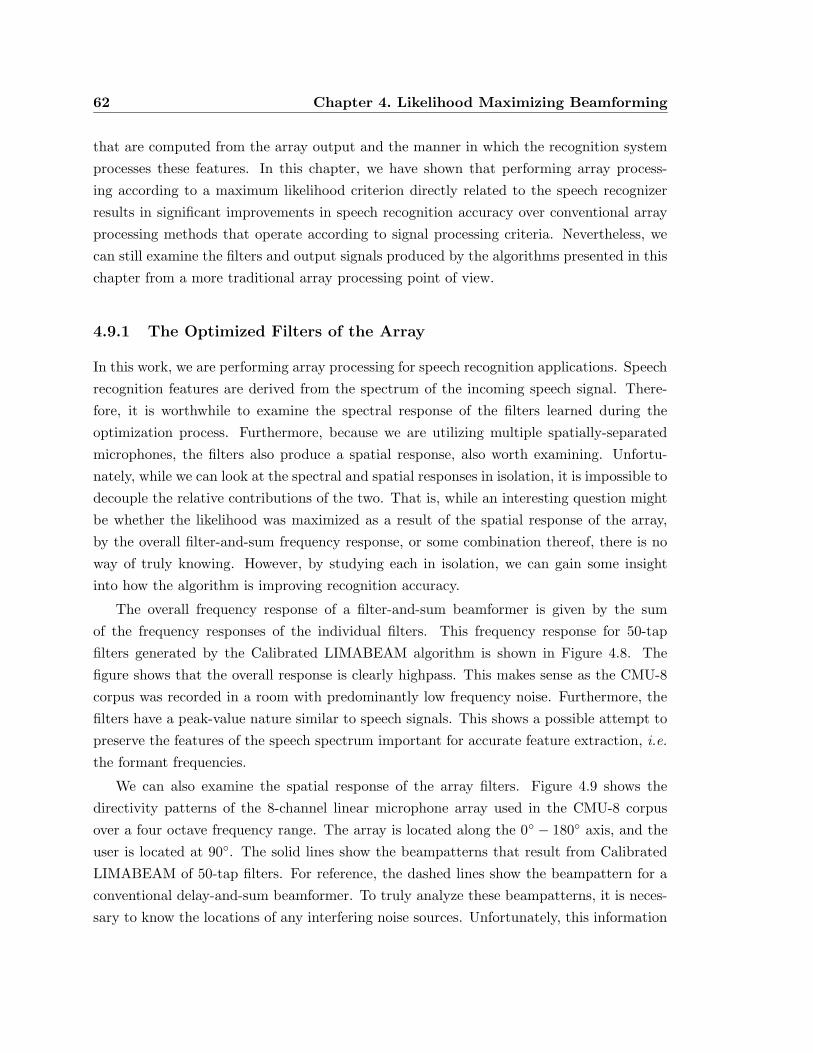
62 Chapter 4. Likelihood Maximizing Beamforming
that are computed from the array output and the manner in which the recognition system
processes these features. In this chapter, we have shown that performing array process-
ing according to a maximum likelihood criterion directly related to the speech recognizer
results in significant improvements in speech recognition accuracy over conventional array
processing methods that operate according to signal processing criteria. Nevertheless, we
can still examine the filters and output signals produced by the algorithms presented in this
chapter from a more traditional array processing point of view.
4.9.1 The Optimized Filters of the Array
In this work, we are performing array processing for speech recognition applications. Speech
recognition features are derived from the spectrum of the incoming speech signal. There-
fore, it is worthwhile to examine the spectral response of the filters learned during the
optimization process. Furthermore, because we are utilizing multiple spatially-separated
microphones, the filters also produce a spatial response, also worth examining. Unfortu-
nately, while we can look at the spectral and spatial responses in isolation, it is impossible to
decouple the relative contributions of the two. That is, while an interesting question might
be whether the likelihood was maximized as a result of the spatial response of the array,
by the overall filter-and-sum frequency response, or some combination thereof, there is no
way of truly knowing. However, by studying each in isolation, we can gain some insight
into how the algorithm is improving recognition accuracy.
The overall frequency response of a filter-and-sum beamformer is given by the sum
of the frequency responses of the individual filters. This frequency response for 50-tap
filters generated by the Calibrated LIMABEAM algorithm is shown in Figure 4.8. The
figure shows that the overall response is clearly highpass. This makes sense as the CMU-8
corpus was recorded in a room with predominantly low frequency noise. Furthermore, the
filters have a peak-value nature similar to speech signals. This shows a possible attempt to
preserve the features of the speech spectrum important for accurate feature extraction, i.e.
the formant frequencies.
We can also examine the spatial response of the array filters. Figure 4.9 shows the
directivity patterns of the 8-channel linear microphone array used in the CMU-8 corpus
over a four octave frequency range. The array is located along the 0◦ − 180◦ axis, and the
user is located at 90◦. The solid lines show the beampatterns that result from Calibrated
LIMABEAM of 50-tap filters. For reference, the dashed lines show the beampattern for a
conventional delay-and-sum beamformer. To truly analyze these beampatterns, it is neces-
sary to know the locations of any interfering noise sources. Unfortunately, this information
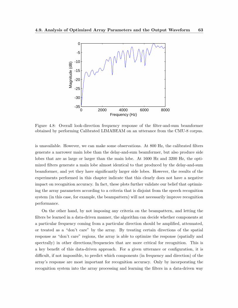
4.9. Analysis of Optimized Array Parameters and the Output Waveform 63
0 2000 4000 6000 8000-35
-30
-25
-20
-15
-10
-5
0
Mag
nitu
de (
dB)
Frequency (Hz)
Figure 4.8: Overall look-direction frequency response of the filter-and-sum beamformerobtained by performing Calibrated LIMABEAM on an utterance from the CMU-8 corpus.
is unavailable. However, we can make some observations. At 800 Hz, the calibrated filters
generate a narrower main lobe than the delay-and-sum beamformer, but also produce side
lobes that are as large or larger than the main lobe. At 1600 Hz and 3200 Hz, the opti-
mized filters generate a main lobe almost identical to that produced by the delay-and-sum
beamformer, and yet they have significantly larger side lobes. However, the results of the
experiments performed in this chapter indicate that this clearly does not have a negative
impact on recognition accuracy. In fact, these plots further validate our belief that optimiz-
ing the array parameters according to a criteria that is disjoint from the speech recognition
system (in this case, for example, the beampattern) will not necessarily improve recognition
performance.
On the other hand, by not imposing any criteria on the beampattern, and letting the
filters be learned in a data-driven manner, the algorithm can decide whether components at
a particular frequency coming from a particular direction should be amplified, attenuated,
or treated as a “don’t care” by the array. By treating certain directions of the spatial
response as “don’t care” regions, the array is able to optimize the response (spatially and
spectrally) in other directions/frequencies that are more critical for recognition. This is
a key benefit of this data-driven approach. For a given utterance or configuration, it is
difficult, if not impossible, to predict which components (in frequency and direction) of the
array’s response are most important for recognition accuracy. Only by incorporating the
recognition system into the array processing and learning the filters in a data-driven way
64 Chapter 4. Likelihood Maximizing Beamforming
0.2
0.4
0.6
0.8
1
30
210
60
240
90
270
120
300
150
330
180 0
0.2
0.4
0.6
0.8
1
30
210
60
240
90
270
120
300
150
330
180 0
(a) 400 Hz (b) 800 Hz
0.2
0.4
0.6
0.8
1
30
210
60
240
90
270
120
300
150
330
180 0
0.2
0.4
0.6
0.8
1
30
210
60
240
90
270
120
300
150
330
180 0
(c) 1600 Hz (d) 3200 Hz
Figure 4.9: Beampatterns of the filter-and-sum beamformer obtained by performing Cali-brated LIMABEAM on an utterance from the CMU-8 corpus.
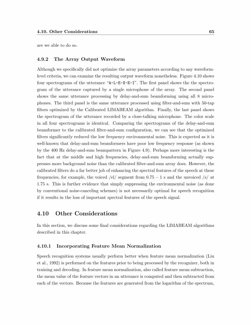
4.10. Other Considerations 65
are we able to do so.
4.9.2 The Array Output Waveform
Although we specifically did not optimize the array parameters according to any waveform-
level criteria, we can examine the resulting output waveform nonetheless. Figure 4.10 shows
four spectrograms of the utterance “A-L-E-X-E-I”. The first panel shows the the spectro-
gram of the utterance captured by a single microphone of the array. The second panel
shows the same utterance processing by delay-and-sum beamforming using all 8 micro-
phones. The third panel is the same utterance processed using filter-and-sum with 50-tap
filters optimized by the Calibrated LIMABEAM algorithm. Finally, the last panel shows
the spectrogram of the utterance recorded by a close-talking microphone. The color scale
in all four spectrograms is identical. Comparing the spectrograms of the delay-and-sum
beamformer to the calibrated filter-and-sum configuration, we can see that the optimized
filters significantly reduced the low frequency environmental noise. This is expected as it is
well-known that delay-and-sum beamformers have poor low frequency response (as shown
by the 400 Hz delay-and-sum beampattern in Figure 4.9). Perhaps more interesting is the
fact that at the middle and high frequencies, delay-and-sum beamforming actually sup-
presses more background noise than the calibrated filter-and-sum array does. However, the
calibrated filters do a far better job of enhancing the spectral features of the speech at these
frequencies, for example, the voiced /el/ segment from 0.75 − 1 s and the unvoiced /s/ at
1.75 s. This is further evidence that simply suppressing the environmental noise (as done
by conventional noise-canceling schemes) is not necessarily optimal for speech recognition
if it results in the loss of important spectral features of the speech signal.
4.10 Other Considerations
In this section, we discuss some final considerations regarding the LIMABEAM algorithms
described in this chapter.
4.10.1 Incorporating Feature Mean Normalization
Speech recognition systems usually perform better when feature mean normalization (Liu
et al., 1992) is performed on the features prior to being processed by the recognizer, both in
training and decoding. In feature mean normalization, also called feature mean subtraction,
the mean value of the feature vectors in an utterance is computed and then subtracted from
each of the vectors. Because the features are generated from the logarithm of the spectrum,

66 Chapter 4. Likelihood Maximizing Beamforming
Time (sec)
Fre
quen
cy (
Hz)
0 0.5 1 1.5 2 2.50
1000
2000
3000
4000
5000
6000
7000
8000
Time (sec)
Fre
quen
cy (
Hz)
0 0.5 1 1.5 2 2.50
1000
2000
3000
4000
5000
6000
7000
8000
(a) single microphone (b) delay-and-sum
Time (sec)
Fre
quen
cy (
Hz)
0 0.5 1 1.5 2 2.50
1000
2000
3000
4000
5000
6000
7000
8000
Time (sec)
Fre
quen
cy (
Hz)
0 0.5 1 1.5 2 2.50
1000
2000
3000
4000
5000
6000
7000
8000
(c) Calibrated LIMABEAM (d) close-talking microphone
Figure 4.10: Spectrograms of an utterance from the CMU-8 corpus obtained using (a) singlemicrophone only, (b) delay-and-sum beamforming (c) Calibrated LIMABEAM, and (d) theclose-talking microphone.
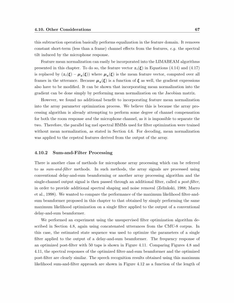
4.10. Other Considerations 67
this subtraction operation basically performs equalization in the feature domain. It removes
constant short-term (less than a frame) channel effects from the features, e.g. the spectral
tilt induced by the microphone response.
Feature mean normalization can easily be incorporated into the LIMABEAM algorithms
presented in this chapter. To do so, the feature vector zi(ξ) in Equations (4.14) and (4.17)
is replaced by (zi(ξ) − µz (ξ)) where µz (ξ) is the mean feature vector, computed over all
frames in the utterance. Because µz (ξ) is a function of ξ as well, the gradient expressions
also have to be modified. It can be shown that incorporating mean normalization into the
gradient can be done simply by performing mean normalization on the Jacobian matrix.
However, we found no additional benefit to incorporating feature mean normalization
into the array parameter optimization process. We believe this is because the array pro-
cessing algorithm is already attempting to perform some degree of channel compensation
for both the room response and the microphone channel, as it is impossible to separate the
two. Therefore, the parallel log mel spectral HMMs used for filter optimization were trained
without mean normalization, as stated in Section 4.6. For decoding, mean normalization
was applied to the cepstral features derived from the output of the array.
4.10.2 Sum-and-Filter Processing
There is another class of methods for microphone array processing which can be referred
to as sum-and-filter methods. In such methods, the array signals are processed using
conventional delay-and-sum beamforming or another array processing algorithm and the
single-channel output signal is then passed through an additional filter, called a post-filter,
in order to provide additional spectral shaping and noise removal (Zelinkski, 1988; Marro
et al., 1998). We wanted to compare the performance of the maximum likelihood filter-and-
sum beamformer proposed in this chapter to that obtained by simply performing the same
maximum likelihood optimization on a single filter applied to the output of a conventional
delay-and-sum beamformer.
We performed an experiment using the unsupervised filter optimization algorithm de-
scribed in Section 4.8, again using concatenated utterances from the CMU-8 corpus. In
this case, the estimated state sequence was used to optimize the parameters of a single
filter applied to the output of a delay-and-sum beamformer. The frequency response of
an optimized post-filter with 50 taps is shown in Figure 4.11. Comparing Figures 4.8 and
4.11, the spectral responses of the optimized filter-and-sum beamformer and the optimized
post-filter are clearly similar. The speech recognition results obtained using this maximum
likelihood sum-and-filter approach are shown in Figure 4.12 as a function of the length of
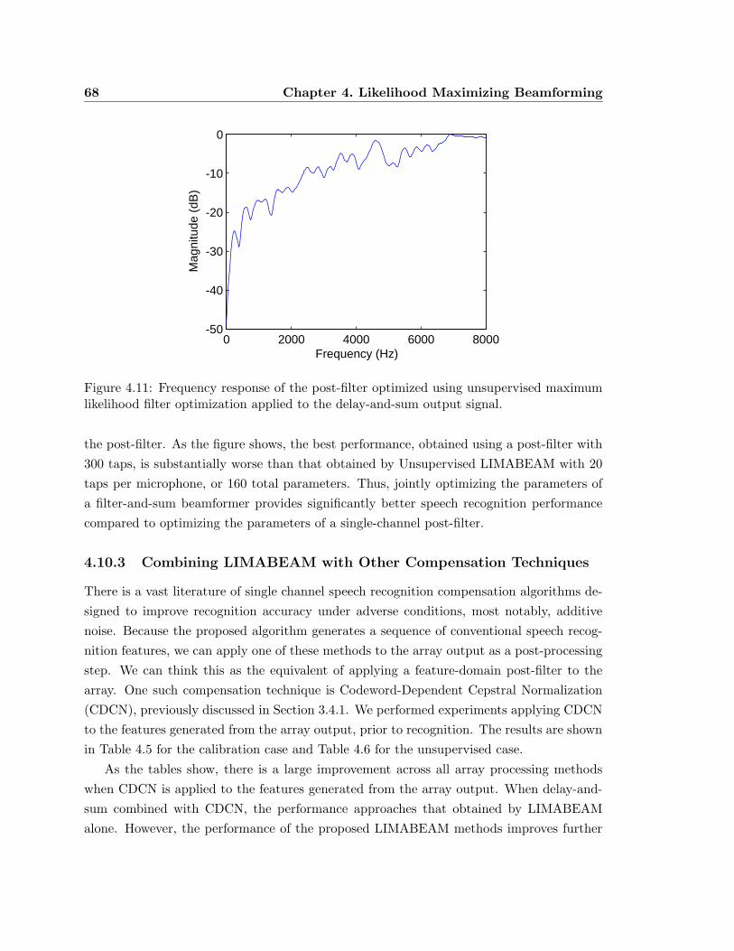
68 Chapter 4. Likelihood Maximizing Beamforming
0 2000 4000 6000 8000-50
-40
-30
-20
-10
0
Mag
nitu
de (
dB)
Frequency (Hz)
Figure 4.11: Frequency response of the post-filter optimized using unsupervised maximumlikelihood filter optimization applied to the delay-and-sum output signal.
the post-filter. As the figure shows, the best performance, obtained using a post-filter with
300 taps, is substantially worse than that obtained by Unsupervised LIMABEAM with 20
taps per microphone, or 160 total parameters. Thus, jointly optimizing the parameters of
a filter-and-sum beamformer provides significantly better speech recognition performance
compared to optimizing the parameters of a single-channel post-filter.
4.10.3 Combining LIMABEAM with Other Compensation Techniques
There is a vast literature of single channel speech recognition compensation algorithms de-
signed to improve recognition accuracy under adverse conditions, most notably, additive
noise. Because the proposed algorithm generates a sequence of conventional speech recog-
nition features, we can apply one of these methods to the array output as a post-processing
step. We can think this as the equivalent of applying a feature-domain post-filter to the
array. One such compensation technique is Codeword-Dependent Cepstral Normalization
(CDCN), previously discussed in Section 3.4.1. We performed experiments applying CDCN
to the features generated from the array output, prior to recognition. The results are shown
in Table 4.5 for the calibration case and Table 4.6 for the unsupervised case.
As the tables show, there is a large improvement across all array processing methods
when CDCN is applied to the features generated from the array output. When delay-and-
sum combined with CDCN, the performance approaches that obtained by LIMABEAM
alone. However, the performance of the proposed LIMABEAM methods improves further
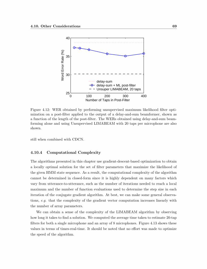
4.10. Other Considerations 69
0 100 200 300 40025
30
35
40
Number of Taps in Post-Filter
Wor
d E
rror
Rat
e (%
)
delay-sumdelay-sum + ML post-filterUnsuper LIMABEAM, 20 taps
Figure 4.12: WER obtained by performing unsupervised maximum likelihood filter opti-mization on a post-filter applied to the output of a delay-and-sum beamformer, shown asa function of the length of the post-filter. The WERs obtained using delay-and-sum beam-forming alone and using Unsupervised LIMABEAM with 20 taps per microphone are alsoshown.
still when combined with CDCN.
4.10.4 Computational Complexity
The algorithms presented in this chapter use gradient-descent-based optimization to obtain
a locally optimal solution for the set of filter parameters that maximize the likelihood of
the given HMM state sequence. As a result, the computational complexity of the algorithm
cannot be determined in closed-form since it is highly dependent on many factors which
vary from utterance-to-utterance, such as the number of iterations needed to reach a local
maximum and the number of function evaluations used to determine the step size in each
iteration of the conjugate gradient algorithm. At best, we can make some general observa-
tions, e.g. that the complexity of the gradient vector computation increases linearly with
the number of array parameters.
We can obtain a sense of the complexity of the LIMABEAM algorithm by observing
how long it takes to find a solution. We computed the average time taken to estimate 20-tap
filters for both a single microphone and an array of 8 microphones. Figure 4.13 shows these
values in terms of times-real-time. It should be noted that no effort was made to optimize
the speed of the algorithm.
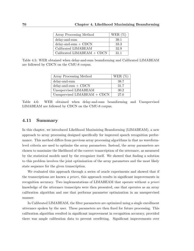
70 Chapter 4. Likelihood Maximizing Beamforming
Array Processing Method WER (%)
delay-and-sum 39.1
delay-and-sum + CDCN 33.3
Calibrated LIMABEAM 32.9
Calibrated LIMABEAM + CDCN 31.1
Table 4.5: WER obtained when delay-and-sum beamforming and Calibrated LIMABEAMare followed by CDCN on the CMU-8 corpus.
Array Processing Method WER (%)
delay-and-sum 38.7
delay-and-sum + CDCN 31.7
Unsupervised LIMABEAM 30.2
Unsupervised LIMABEAM + CDCN 27.0
Table 4.6: WER obtained when delay-and-sum beamforming and UnsupervisedLIMABEAM are followed by CDCN on the CMU-8 corpus.
4.11 Summary
In this chapter, we introduced Likelihood Maximizing Beamforming (LIMABEAM), a new
approach to array processing designed specifically for improved speech recognition perfor-
mance. This method differs from previous array processing algorithms in that no waveform-
level criteria are used to optimize the array parameters. Instead, the array parameters are
chosen to maximize the likelihood of the correct transcription of the utterance, as measured
by the statistical models used by the recognizer itself. We showed that finding a solution
to this problem involves the joint optimization of the array parameters and the most likely
state sequence for the given transcription.
We evaluated this approach through a series of oracle experiments and showed that if
the transcriptions are known a priori , this approach results in significant improvements in
recognition accuracy. Two implementations of LIMABEAM that operate without a priori
knowledge of the utterance transcripts were then presented, one that operates as an array
calibration algorithm and one that performs parameter optimization in an unsupervised
manner.
In Calibrated LIMABEAM, the filter parameters are optimized using a single enrollment
utterance spoken by the user. These parameters are then fixed for future processing. This
calibration algorithm resulted in significant improvement in recognition accuracy, provided
there was ample calibration data to prevent overfitting. Significant improvements over
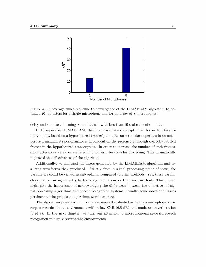
4.11. Summary 71
1 80
10
20
30
40
50
xRT
Number of Microphones
Figure 4.13: Average times-real-time to convergence of the LIMABEAM algorithm to op-timize 20-tap filters for a single microphone and for an array of 8 microphones.
delay-and-sum beamforming were obtained with less than 10 s of calibration data.
In Unsupervised LIMABEAM, the filter parameters are optimized for each utterance
individually, based on a hypothesized transcription. Because this data operates in an unsu-
pervised manner, its performance is dependent on the presence of enough correctly labeled
frames in the hypothesized transcription. In order to increase the number of such frames,
short utterances were concatenated into longer utterances for processing. This dramatically
improved the effectiveness of the algorithm.
Additionally, we analyzed the filters generated by the LIMABEAM algorithm and re-
sulting waveforms they produced. Strictly from a signal processing point of view, the
parameters could be viewed as sub-optimal compared to other methods. Yet, these param-
eters resulted in significantly better recognition accuracy than such methods. This further
highlights the importance of acknowledging the differences between the objectives of sig-
nal processing algorithms and speech recognition systems. Finally, some additional issues
pertinent to the proposed algorithms were discussed.
The algorithms presented in this chapter were all evaluated using the a microphone array
corpus recorded in an environment with a low SNR (6.5 dB) and moderate reverberation
(0.24 s). In the next chapter, we turn our attention to microphone-array-based speech
recognition in highly reverberant environments.

Chapter 5
Subband-Likelihood Maximizing
Beamforming
5.1 Introduction
In the previous chapter, a microphone array processing framework for speech recognition
applications was presented in which the parameters of a filter-and-sum beamformer were
optimized according to the same objective criterion used by the recognition system itself.
In doing so, we were able to achieve significant improvements over conventional microphone
array processing algorithms that operate according to traditional signal processing criteria.
The experiments performed in the previous chapter showed that this approach is capable
of good performance in noisy environments with moderate reverberation. The speech data
used in the experiments were recorded in a room with a reverberation time of 0.24 s and
had an average SNR of 6.5 dB.
Although the objective function is significantly different from those used by conventional
adaptive filtering schemes, the LIMABEAM algorithm is nevertheless a gradient-descent-
based LMS type of algorithm. Conventional LMS adaptive filtering algorithms are known
to exhibit poor convergence behavior when the input signals are highly correlated and the
filter length is long (Haykin, 2002). Unfortunately, both of these conditions are generally
present in highly reverberant environments. Therefore, it is unclear whether the algorithms
proposed in this thesis will be effective in such environments, or if the performance will be
plagued by the same poor convergence issues that hinder more traditional adaptive filtering
algorithms.
In the following section, the performance of the LIMABEAM approach is evaluated
in an environment with significant reverberation. We will see that although small im-
73
74 Chapter 5. Subband-Likelihood Maximizing Beamforming
provements are achieved, the existing adaptive filtering architecture is indeed inadequate to
effectively improve speech recognition performance in such environments. We then examine
the principles of subband filtering and explore its potential as a means of compensation for
the distortions caused by long reverberation times. The remainder of the chapter is spent
describing how subband filtering can be incorporated into the speech-recognizer-based max-
imum likelihood framework established in Chapter 4.
5.2 LIMABEAM in Highly Reverberant Environments
In this section we evaluate the Likelihood Maximizing Beamforming approach described in
the previous chapter for use in highly reverberant operating environments. To do so, we will
use the 7-microphone reverberant WSJ corpora described in Chapter 3. These corpora were
created by convolving the WSJ test set with a series of room impulse responses recorded in
rooms with reverberation times ranging from 0.3 s to 1.3 s.
In this section we limit our experiments to the data captured in a room with a reverber-
ation time of 0.47 s, approximately twice as long as the reverberation time of the CMU-8
corpus used in the previous chapter. We refer to this corpus as WSJ0.47.
The Calibrated LIMABEAM algorithm described in Section 4.7 was performed on the
WSJ0.47 corpus. For each speaker, a single utterance was chosen at random from the utter-
ances that were at least 10 s in duration. As before, the known transcription and features
derived from delay-and-sum processing were used to generate the target state sequence. A
filter-and-sum beamformer was then optimized and used to process the remaining utter-
ances of that speaker. The recognition system used for decoding was the same one used in
the previous chapter. Figure 5.1 shows the WER obtained using this calibration approach
for different filter lengths. The baseline WER obtained from delay-and-sum processing is
also shown.
This figure looks similar to Figure 4.5, the results of the calibration experiment in
the previous chapter. In that chapter, we attributed the poor performance to overfitting.
When many parameters are learned from only a small amount of calibration data, filters
are generated that do not generalize well to unseen test data. Recall that increasing the
amount of calibration data from 3.3 s to 8.3 s significantly improved the performance of the
calibration algorithm when longer filters were optimized.
We can try the same approach to improve the performance here as well. Table 5.1 shows
the performance of the calibration algorithm when 100-tap FIR filters are optimized using
additional calibration data.
In this case, increasing the amount of calibration data does not significantly improve
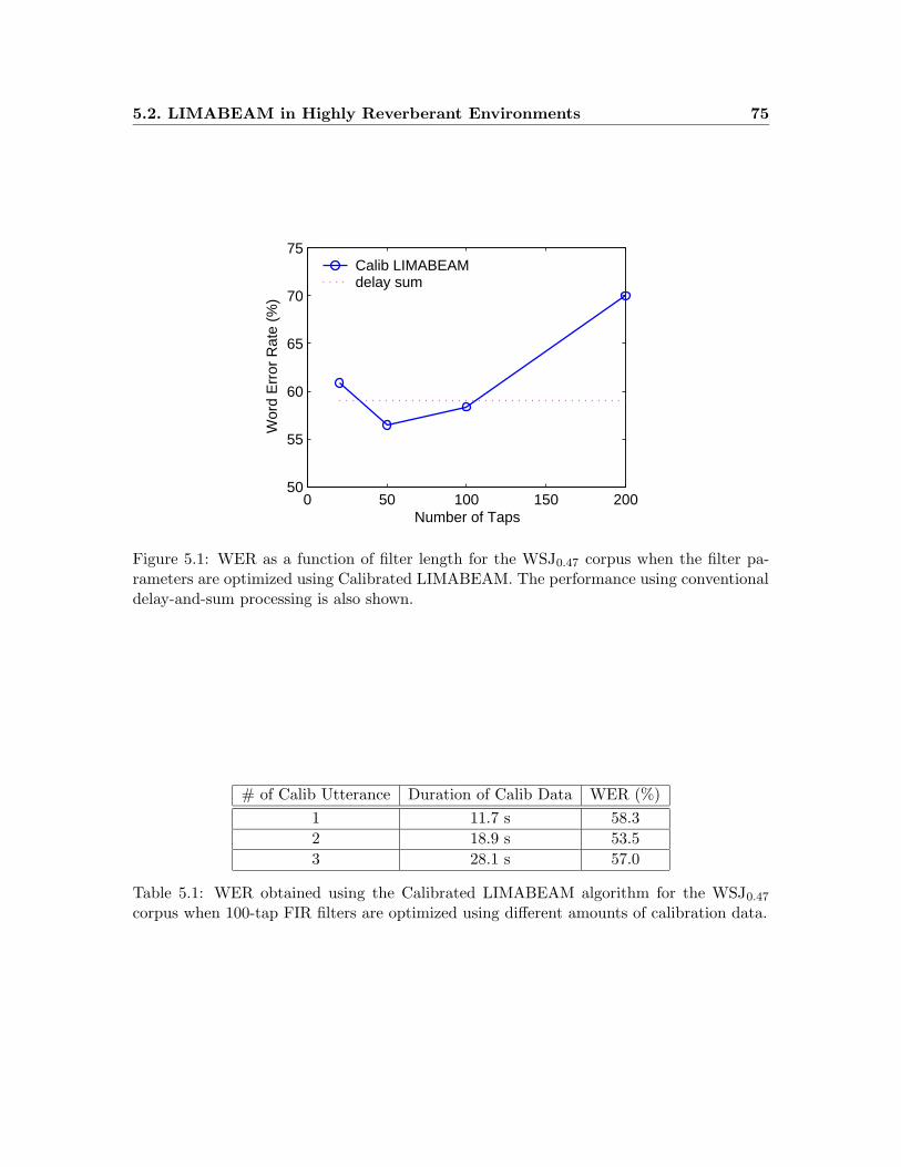
5.2. LIMABEAM in Highly Reverberant Environments 75
0 50 100 150 20050
55
60
65
70
75
Number of Taps
Wor
d E
rror
Rat
e (%
)Calib LIMABEAMdelay sum
Figure 5.1: WER as a function of filter length for the WSJ0.47 corpus when the filter pa-rameters are optimized using Calibrated LIMABEAM. The performance using conventionaldelay-and-sum processing is also shown.
# of Calib Utterance Duration of Calib Data WER (%)
1 11.7 s 58.3
2 18.9 s 53.5
3 28.1 s 57.0
Table 5.1: WER obtained using the Calibrated LIMABEAM algorithm for the WSJ0.47
corpus when 100-tap FIR filters are optimized using different amounts of calibration data.
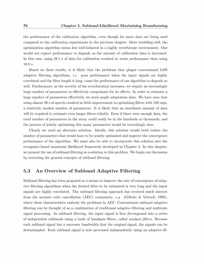
76 Chapter 5. Subband-Likelihood Maximizing Beamforming
the performance of the calibration algorithm, even though far more data are being used
compared to the calibration experiments in the previous chapter. More troubling still, the
optimization algorithm seems less well-behaved in a highly reverberant environment. One
would not expect performance to degrade as the amount of calibration data is increased.
In this case, using 28.1 s of data for calibration resulted in worse performance than using
18.9 s.
Based on these results, it is likely that the problems that plague conventional LMS
adaptive filtering algorithms, i.e. poor performance when the input signals are highly
correlated and the filter length is long, cause the performance of our algorithm to degrade as
well. Furthermore, as the severity of the reverberation increases, we require an increasingly
large number of parameters to effectively compensate for its effects. In order to estimate a
large number of parameters effectively, we need ample adaptation data. We have seen that
using almost 30 s of speech resulted in little improvement in optimizing filters with 100 taps,
a relatively modest number of parameters. It is likely that an inordinate amount of data
will be required to estimate even longer filters reliably. Even if there were enough data, the
total number of parameters in the array could easily be in the hundreds or thousands, and
the process of jointly optimizing this many parameters would be exceedingly slow.
Clearly we need an alternate solution. Ideally, this solution would both reduce the
number of parameters that would have to be jointly optimized and improve the convergence
performance of the algorithm. We must also be able to incorporate this solution into the
recognizer-based maximum likelihood framework developed in Chapter 4. In this chapter,
we present the use of subband filtering as a solution to this problem. We begin our discussion
by reviewing the general concepts of subband filtering.
5.3 An Overview of Subband Adaptive Filtering
Subband filtering has been proposed as a means to improve the rate of convergence of adap-
tive filtering algorithms when the desired filter to be estimated is very long and the input
signals are highly correlated. The subband filtering approach has received much interest
from the acoustic echo cancellation (AEC) community, e.g. (Gilloire & Vetterli, 1992),
where these characteristics embody the problems in AEC. Conventional subband adaptive
filtering can be thought of as a combination of traditional adaptive filtering and multirate
signal processing. In subband filtering, the input signal is first decomposed into a series
of independent subbands using a bank of bandpass filters, called analysis filters. Because
each subband signal has a narrower bandwidth that the original signal, the signals can be
downsampled. Each subband signal is now processed independently using an adaptive fil-
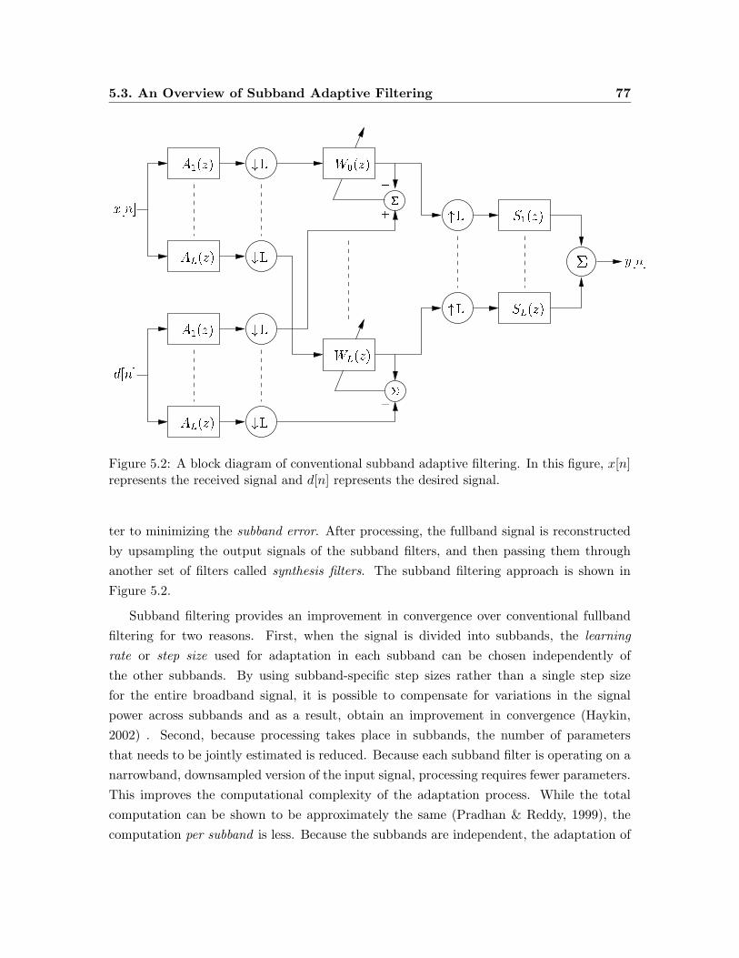
5.3. An Overview of Subband Adaptive Filtering 77
���������
�������
� �
� �
� �
��� �����
� � �����
��� ����� � �
� � �����
� � �����
��� �����
���
���
�
��
��
�
�
��� ���
� � ���
� � ���
Figure 5.2: A block diagram of conventional subband adaptive filtering. In this figure, x[n]represents the received signal and d[n] represents the desired signal.
ter to minimizing the subband error. After processing, the fullband signal is reconstructed
by upsampling the output signals of the subband filters, and then passing them through
another set of filters called synthesis filters. The subband filtering approach is shown in
Figure 5.2.
Subband filtering provides an improvement in convergence over conventional fullband
filtering for two reasons. First, when the signal is divided into subbands, the learning
rate or step size used for adaptation in each subband can be chosen independently of
the other subbands. By using subband-specific step sizes rather than a single step size
for the entire broadband signal, it is possible to compensate for variations in the signal
power across subbands and as a result, obtain an improvement in convergence (Haykin,
2002) . Second, because processing takes place in subbands, the number of parameters
that needs to be jointly estimated is reduced. Because each subband filter is operating on a
narrowband, downsampled version of the input signal, processing requires fewer parameters.
This improves the computational complexity of the adaptation process. While the total
computation can be shown to be approximately the same (Pradhan & Reddy, 1999), the
computation per subband is less. Because the subbands are independent, the adaptation of
78 Chapter 5. Subband-Likelihood Maximizing Beamforming
the different subband filters can be performed in parallel.
Subband filtering has been applied to microphone array processing by other researchers.
However, all proposed methods have generated subband versions of conventional micro-
phone array algorithms. For example, several researchers have proposed subband versions
of the Generalized Sidelobe Canceller, e.g. (Neo & Farhang-Boroujeny, 2001; Liu et al.,
2001). However, subband filtering is simply a way improving the efficiency of the filter
adaptation process. Its success or failure is still dependent on the objective criteria used
for the adaptation. As we have seen, algorithms which rely on waveform-level criteria for
filter adaptation do not to improve recognition accuracy significantly, and as such, we can
expect the same performance from their subband counterparts.
5.4 Subband Filtering for Microphone-array-based Speech
Recognition
The attributes that make subband processing useful for applications such as AEC make
it similarly appealing for use in recognizing speech that has been distorted by significant
amounts of reverberation. However, subband processing is a means of improving the ef-
ficiency of a given algorithm or approach, not an algorithm unto itself. Therefore, unless
the original fullband algorithm improves recognition accuracy, we cannot expect the sub-
band version of the algorithm to do so either. It will simply be a more efficient way to
generate poor results! Thus, the goal of this chapter is to develop a microphone array
processing algorithm which exploits the benefits of subband filtering while maintaining the
recognizer-based maximum likelihood framework developed in the previous chapter.
In this section, we begin to address this goal, by demonstrating that subband filtering
can be readily incorporated into the processing already performed by the recognizer for
feature extraction.
5.4.1 Incorporating Subband Processing into the ASR Front-End
As described in Section 2.2.1, a Short-Time Fourier Transform (STFT) is used for spectral
estimation in the feature extraction process of most recognition systems. The incoming
waveform is segmented into a series of overlapping frames. In this work, a frame length of 25
ms is used and the starting sample of the frame is shifted 10 ms between consecutive frames.
The samples in the frame are then windowed using a Hamming window and transformed to
the frequency domain using a DFT. This process generates a series of short-time spectral
vectors. Features are then extracted from these vectors through a series of additional
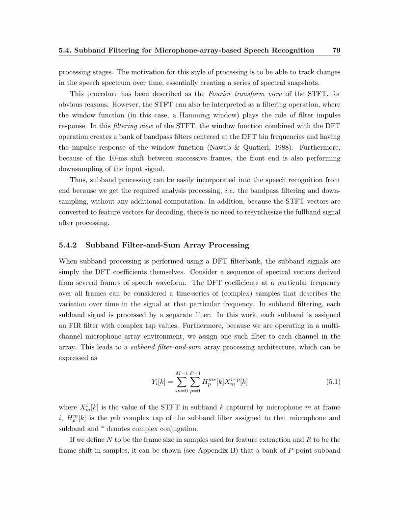
5.4. Subband Filtering for Microphone-array-based Speech Recognition 79
processing stages. The motivation for this style of processing is to be able to track changes
in the speech spectrum over time, essentially creating a series of spectral snapshots.
This procedure has been described as the Fourier transform view of the STFT, for
obvious reasons. However, the STFT can also be interpreted as a filtering operation, where
the window function (in this case, a Hamming window) plays the role of filter impulse
response. In this filtering view of the STFT, the window function combined with the DFT
operation creates a bank of bandpass filters centered at the DFT bin frequencies and having
the impulse response of the window function (Nawab & Quatieri, 1988). Furthermore,
because of the 10-ms shift between successive frames, the front end is also performing
downsampling of the input signal.
Thus, subband processing can be easily incorporated into the speech recognition front
end because we get the required analysis processing, i.e. the bandpass filtering and down-
sampling, without any additional computation. In addition, because the STFT vectors are
converted to feature vectors for decoding, there is no need to resynthesize the fullband signal
after processing.
5.4.2 Subband Filter-and-Sum Array Processing
When subband processing is performed using a DFT filterbank, the subband signals are
simply the DFT coefficients themselves. Consider a sequence of spectral vectors derived
from several frames of speech waveform. The DFT coefficients at a particular frequency
over all frames can be considered a time-series of (complex) samples that describes the
variation over time in the signal at that particular frequency. In subband filtering, each
subband signal is processed by a separate filter. In this work, each subband is assigned
an FIR filter with complex tap values. Furthermore, because we are operating in a multi-
channel microphone array environment, we assign one such filter to each channel in the
array. This leads to a subband filter-and-sum array processing architecture, which can be
expressed as
Yi[k] =
M−1∑
m=0
P−1∑
p=0
Hm∗p [k]X i−p
m [k] (5.1)
where X im[k] is the value of the STFT in subband k captured by microphone m at frame
i, Hmp [k] is the pth complex tap of the subband filter assigned to that microphone and
subband and ∗ denotes complex conjugation.
If we define N to be the frame size in samples used for feature extraction and R to be the
frame shift in samples, it can be shown (see Appendix B) that a bank of P -point subband
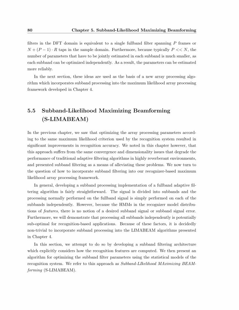
80 Chapter 5. Subband-Likelihood Maximizing Beamforming
filters in the DFT domain is equivalent to a single fullband filter spanning P frames or
N + (P − 1) · R taps in the sample domain. Furthermore, because typically P << N , the
number of parameters that have to be jointly estimated in each subband is much smaller, as
each subband can be optimized independently. As a result, the parameters can be estimated
more reliably.
In the next section, these ideas are used as the basis of a new array processing algo-
rithm which incorporates subband processing into the maximum likelihood array processing
framework developed in Chapter 4.
5.5 Subband-Likelihood Maximizing Beamforming
(S-LIMABEAM)
In the previous chapter, we saw that optimizing the array processing parameters accord-
ing to the same maximum likelihood criterion used by the recognition system resulted in
significant improvements in recognition accuracy. We noted in this chapter however, that
this approach suffers from the same convergence and dimensionality issues that degrade the
performance of traditional adaptive filtering algorithms in highly reverberant environments,
and presented subband filtering as a means of alleviating these problems. We now turn to
the question of how to incorporate subband filtering into our recognizer-based maximum
likelihood array processing framework.
In general, developing a subband processing implementation of a fullband adaptive fil-
tering algorithm is fairly straightforward. The signal is divided into subbands and the
processing normally performed on the fullband signal is simply performed on each of the
subbands independently. However, because the HMMs in the recognizer model distribu-
tions of features, there is no notion of a desired subband signal or subband signal error.
Furthermore, we will demonstrate that processing all subbands independently is potentially
sub-optimal for recognition-based applications. Because of these factors, it is decidedly
non-trivial to incorporate subband processing into the LIMABEAM algorithms presented
in Chapter 4.
In this section, we attempt to do so by developing a subband filtering architecture
which explicitly considers how the recognition features are computed. We then present an
algorithm for optimizing the subband filter parameters using the statistical models of the
recognition system. We refer to this approach as Subband-LIkelihood MAximizing BEAM-
forming (S-LIMABEAM).
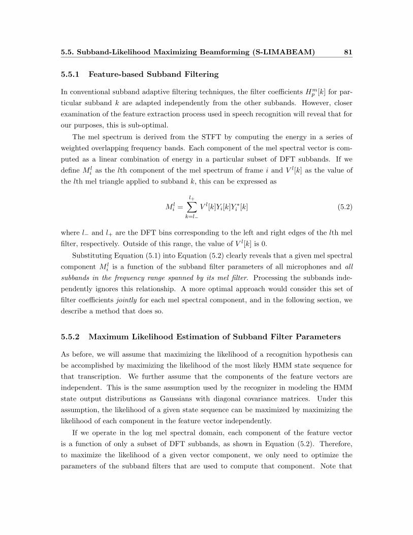
5.5. Subband-Likelihood Maximizing Beamforming (S-LIMABEAM) 81
5.5.1 Feature-based Subband Filtering
In conventional subband adaptive filtering techniques, the filter coefficients Hmp [k] for par-
ticular subband k are adapted independently from the other subbands. However, closer
examination of the feature extraction process used in speech recognition will reveal that for
our purposes, this is sub-optimal.
The mel spectrum is derived from the STFT by computing the energy in a series of
weighted overlapping frequency bands. Each component of the mel spectral vector is com-
puted as a linear combination of energy in a particular subset of DFT subbands. If we
define M li as the lth component of the mel spectrum of frame i and V l[k] as the value of
the lth mel triangle applied to subband k, this can be expressed as
M li =
l+∑
k=l−
V l[k]Yi[k]Y ∗i [k] (5.2)
where l− and l+ are the DFT bins corresponding to the left and right edges of the lth mel
filter, respectively. Outside of this range, the value of V l[k] is 0.
Substituting Equation (5.1) into Equation (5.2) clearly reveals that a given mel spectral
component M li is a function of the subband filter parameters of all microphones and all
subbands in the frequency range spanned by its mel filter. Processing the subbands inde-
pendently ignores this relationship. A more optimal approach would consider this set of
filter coefficients jointly for each mel spectral component, and in the following section, we
describe a method that does so.
5.5.2 Maximum Likelihood Estimation of Subband Filter Parameters
As before, we will assume that maximizing the likelihood of a recognition hypothesis can
be accomplished by maximizing the likelihood of the most likely HMM state sequence for
that transcription. We further assume that the components of the feature vectors are
independent. This is the same assumption used by the recognizer in modeling the HMM
state output distributions as Gaussians with diagonal covariance matrices. Under this
assumption, the likelihood of a given state sequence can be maximized by maximizing the
likelihood of each component in the feature vector independently.
If we operate in the log mel spectral domain, each component of the feature vector
is a function of only a subset of DFT subbands, as shown in Equation (5.2). Therefore,
to maximize the likelihood of a given vector component, we only need to optimize the
parameters of the subband filters that are used to compute that component. Note that
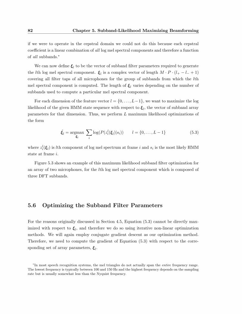
82 Chapter 5. Subband-Likelihood Maximizing Beamforming
if we were to operate in the cepstral domain we could not do this because each cepstral
coefficient is a linear combination of all log mel spectral components and therefore a function
of all subbands.∗
We can now define ξl to be the vector of subband filter parameters required to generate
the lth log mel spectral component. ξl is a complex vector of length M · P · (l+ − l− + 1)
covering all filter taps of all microphones for the group of subbands from which the lth
mel spectral component is computed. The length of ξl varies depending on the number of
subbands used to compute a particular mel spectral component.
For each dimension of the feature vector l = {0, . . . , L−1}, we want to maximize the log
likelihood of the given HMM state sequence with respect to ξl, the vector of subband array
parameters for that dimension. Thus, we perform L maximum likelihood optimizations of
the form
ξl = argmaxξl
∑
i
log(P (zli(ξl)|si)) l = {0, . . . , L− 1} (5.3)
where zli(ξl) is lth component of log mel spectrum at frame i and si is the most likely HMM
state at frame i.
Figure 5.3 shows an example of this maximum likelihood subband filter optimization for
an array of two microphones, for the lth log mel spectral component which is composed of
three DFT subbands.
5.6 Optimizing the Subband Filter Parameters
For the reasons originally discussed in Section 4.5, Equation (5.3) cannot be directly max-
imized with respect to ξl, and therefore we do so using iterative non-linear optimization
methods. We will again employ conjugate gradient descent as our optimization method.
Therefore, we need to compute the gradient of Equation (5.3) with respect to the corre-
sponding set of array parameters, ξl.
∗In most speech recognition systems, the mel triangles do not actually span the entire frequency range.The lowest frequency is typically between 100 and 150 Hz and the highest frequency depends on the samplingrate but is usually somewhat less than the Nyquist frequency.
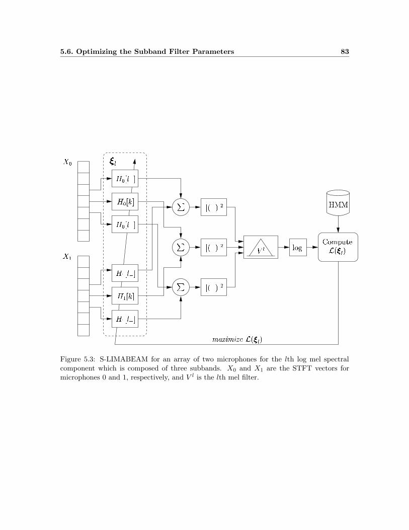
5.6. Optimizing the Subband Filter Parameters 83
�����
������� ������������� ��� � �
���! #"�$&%
���! #"(')%
���* #+,%
�.-/ #+,%
�.-0 #"�$&%
�.-0 #"(')%
� ��� � �
� ��� � �
132
4�5/68794�7;:*< ����� �
=
=
=
> ��?@
A �
AB-
Figure 5.3: S-LIMABEAM for an array of two microphones for the lth log mel spectralcomponent which is composed of three subbands. X0 and X1 are the STFT vectors formicrophones 0 and 1, respectively, and V l is the lth mel filter.
84 Chapter 5. Subband-Likelihood Maximizing Beamforming
5.6.1 Gaussian State Output Distributions
If the HMM state output distributions are assumed to be Gaussian, then the log-likelihood
expression in Equation (5.3) can be written as
L(ξl) =∑
i
−1
2
(zli(ξl)− µli
)2
σl 2i+ κli (5.4)
where µli and σl 2i are the mean and variance of the lth dimension of the Gaussian of state
si and κli is a normalizing constant. The gradient of Equation (5.4) can be expressed as
∇ξlL(ξl) = −∑
i=0
(zli(ξl)− µli
)
σl 2i
∂zli(ξl)
∂ξl(5.5)
where ∂zli(ξl)/∂ξl is the gradient vector. In the previous chapter, we were differentiating the
full feature vector with respect to a vector of array parameters, which resulted in a Jacobian
matrix. Here, we are differentiating only a single component of the feature vector, i.e. a
scalar, with respect to the array parameters, which produces a gradient vector. The gradient
vector is a complex vector with dimension that varies according to the log mel spectral
component. For the lth component, the length of the gradient vector is M ·P · (l+− l−+1).
The complete derivation of the gradient vector is given in Appendix C
5.6.2 Mixture of Gaussians State Output Distributions
In the case where the state densities are mixtures of Gaussians, the log-likelihood expression
is expressed as
L(ξl) =N−1∑
i=0
log
{K∑
k=1
exp
(−1
2
(zli(ξl)− µik[l]
)2
σl 2ik+ log(αik) + κlik
)}(5.6)
In a similar manner as before, we will use Glik(ξl) to represent the term inside the exp()
operator, giving the following more compact representation of the log likelihood
L(ξl) =N−1∑
i=0
log
{K∑
k=1
exp(Glik(ξl)
)}(5.7)
The derivation of the gradient is very similar to the derivation of the Jacobian matrix
5.7. Analysis of the Dimensionality of Subband Filtering 85
in the fullband filter case in Chapter 4. The expression is
∇ξL(ξ) = −∑
i
K∑
k=1
γlik(ξl)
(zli(ξl)− µlik
)
σl 2ik
∂zli(ξl)
∂ξl(5.8)
where γlik(ξl) is the a posteriori probability that the lth dimension of the kth Gaussian in
the mixture modeling state si generated the observed log mel spectral component zli(ξl).
Because we are doing component-wise optimization, there are L separate optimizations
performed, one for each dimension of the log mel spectral vector. Again, because we are
performing subband processing, there are far fewer parameters to optimize per optimization
than in the fullband case. Because the mel triangles are spaced along the frequency axis so
that adjacent triangles overlap each other by 50%, each DFT subband contributes to the
value of two mel spectral components. By processing the DFT subbands jointly within each
mel component, but independently across mel components, the optimization of the complete
log mel spectral vector has twice as many degrees of freedom compared to conventional
subband filtering schemes.
In the next section we analyze the number of parameters required in the subband filtering
approach compared to the number of parameter required in a more conventional fullband
filtering approach.
5.7 Analysis of the Dimensionality of Subband Filtering
As stated earlier, one of the major benefits of subband filtering schemes is a reduction in
the number of parameters that have to be jointly estimated. Simply put, in the subband
approach, a single filter whose parameters must be optimized jointly is replaced by multiple
filters that can be optimized independently, each with fewer parameters. In this section we
highlight the savings in parameters obtained for the specific case of subband filtering using
the bandpass filtering and downsampling inherent in the feature extraction process.
In the S-LIMABEAM scheme described in Section 5.5, an independent optimization is
performed for each dimension of the log mel spectral vector. The number of parameters to
be learned in each optimization depends on the mel filter used to compute the particular
vector component. The value can be computed as M · P · (l+ − l− + 1) where M is the
number of microphones, P is the number of taps per filter, and l− and l+ are the lowest and
highest bins, respectively, in the lth mel filter. Because the filter taps are complex valued,
the total number of parameters to be optimized is actually twice this number, as both the
real and imaginary components of each tap must be estimated.
86 Chapter 5. Subband-Likelihood Maximizing Beamforming
As shown in Appendix B, a bank of P -point subband filters is equivalent to a single
fullband filter spanning P frames or N + (P − 1) ·R samples, where N is the frame size and
R is the frame shift in samples. In this work, N = 400 and R = 160, corresponding to a
25-ms window and 10-ms shift for speech sampled at 16 kHz. A total of 256 subbands were
computed from a 512-point DFT. The features were derived from 40 mel triangles covering
a frequency range from 125 Hz to 6850 Hz, and the number of subbands in each triangle
ranged from 2 to 23. These values are typical for state-of-the-art HMM speech recognition
systems. Thus, the maximum number of free parameters that have to jointly optimized is
M · P · 23 · 2, or 46 · P per microphone.
Figure 5.4 shows the number of parameters per microphone that need to be jointly
optimized as a function of the effective filter length in frames. The dashed line shows
the number of parameters required for a fullband time-domain FIR filter, as used in the
previous chapter. The solid line shows the number of parameters required to optimize the
vector component that corresponds to the widest mel filter. This represents the maximum
number of parameters that need to be estimated jointly for the proposed feature-based
subband filtering scheme. Finally, the dotted line shows the total number of parameters
over all dimensions of the feature vector that need to be optimized using this method. Thus,
the total number of parameters that need to be optimized is actually greater than in the
fullband case. However, because the parameters for each dimension of the feature vector
are optimized independently, the number of parameters that need to be jointly estimated
is greatly reduced.
5.8 Applying S-LIMABEAM to Reverberant Speech
In this chapter a new method has been described in which filter parameters are optimized
in subband domain to maximize the likelihood of a given transcription. This method can be
readily incorporated into the two algorithms presented in Chapter 4. The only significant
change to the algorithms is that the single optimization over all filter parameters for all
microphones in the original algorithms is replaced by L independent optimizations, where
L is the length of the log mel spectral feature vector.
In the following section, we evaluate the performance of the described subband filter
architecture in a reverberant environment by optimizing the subband parameters using
oracle state sequences. As before, this will define the upper bound on the performance of
the subband approach. We then perform experiments to evaluate the performance of the
subband filtering approach when it is incorporated into both the array calibration algorithm
and the unsupervised array processing algorithm.
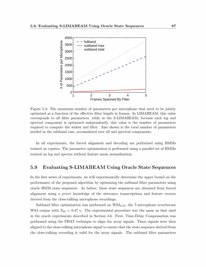
5.9. Evaluating S-LIMABEAM Using Oracle State Sequences 87
1 2 3 4 50
500
1000
1500
2000
2500
3000
3500
4000
Frames Spanned By Filter
# of
Par
amet
ers
per
Mic
roph
one fullband
subband maxsubband total
Figure 5.4: The maximum number of parameters per microphone that need to be jointlyoptimized as a function of the effective filter length in frames. In LIMABEAM, this valuecorresponds to all filter parameters, while in the S-LIMABEAM, because each log melspectral component is optimized independently, this value is the number of parametersrequired to compute the widest mel filter. Also shown is the total number of parametersneeded in the subband case, accumulated over all mel spectral components.
In all experiments, the forced alignment and decoding are performed using HMMs
trained on cepstra. The parameter optimization is performed using a parallel set of HMMs
trained on log mel spectra without feature mean normalization.
5.9 Evaluating S-LIMABEAM Using Oracle State Sequences
In the first series of experiments, we will experimentally determine the upper bound on the
performance of the proposed algorithm by optimizing the subband filter parameters using
oracle HMM state sequences. As before, these state sequences are obtained from forced
alignment using a priori knowledge of the utterance transcriptions and feature vectors
derived from the close-talking microphone recordings.
Subband filter optimization was performed on WSJ0.47, the 7-microphone reverberant
WSJ corpus with T60 = 0.47 s. The experimental procedure was the same as that used
in the oracle experiments described in Section 4.6. First, Time-Delay Compensation was
performed using the PHAT technique to align the array signals. These signals were then
aligned to the close-talking microphone signal to ensure that the state sequence derived from
the close-talking recording is valid for the array signals. The subband filter parameters
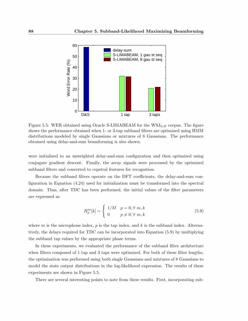
88 Chapter 5. Subband-Likelihood Maximizing Beamforming
D&S 1 tap 3 taps0
10
20
30
40
50
60
Wor
d E
rror
Rat
e (%
)
delay-sumS-LIMABEAM, 1 gau st seqS-LIMABEAM, 8 gau st seq
Figure 5.5: WER obtained using Oracle S-LIMABEAM for the WSJ0.47 corpus. The figureshows the performance obtained when 1- or 3-tap subband filters are optimized using HMMdistributions modeled by single Gaussians or mixtures of 8 Gaussians. The performanceobtained using delay-and-sum beamforming is also shown.
were initialized to an unweighted delay-and-sum configuration and then optimized using
conjugate gradient descent. Finally, the array signals were processed by the optimized
subband filters and converted to cepstral features for recognition.
Because the subband filters operate on the DFT coefficients, the delay-and-sum con-
figuration in Equation (4.24) used for initialization must be transformed into the spectral
domain. Thus, after TDC has been performed, the initial values of the filter parameters
are expressed as
Hmp [k] =
{1/M p = 0, ∀ m, k0 p 6= 0, ∀ m, k
(5.9)
where m is the microphone index, p is the tap index, and k is the subband index. Alterna-
tively, the delays required for TDC can be incorporated into Equation (5.9) by multiplying
the subband tap values by the appropriate phase terms.
In these experiments, we evaluated the performance of the subband filter architecture
when filters composed of 1 tap and 3 taps were optimized. For both of these filter lengths,
the optimization was performed using both single Gaussians and mixtures of 8 Gaussians to
model the state output distributions in the log-likelihood expression. The results of these
experiments are shown in Figure 5.5.
There are several interesting points to note from these results. First, incorporating sub-
5.10. The Calibrated S-LIMABEAM Algorithm 89
band filtering into the maximum likelihood parameter optimization framework developed in
Chapter 4 has the potential to dramatically improve recognition performance in reverberant
environments. The figure shows that relative improvements over delay-and-sum beamform-
ing of more than 45% are possible with only a single tap per subband filter, and of more
than 60% are possible with 3 taps per filter.
Second, significant improvements can be obtained with only a single tap in the subband
domain. With only a single tap for each subband filter, no processing across frames is
occurring as each subband component is simply multiplied by a weight. This shows that
in a microphone array scenario, significant improvements can be achieved without inverse
filtering. If inverse filtering were required, one would expect that filters spanning several
frames would be necessary, and little improvement in recognition accuracy would be seen
with only a single tap. The figure does show however, that when the 3 taps are used and
processing does occur across time, substantial additional improvement is possible.
Finally, these plots show that, at least for the oracle case, there is not a significant
advantage to using more complicated densities to model the state output distributions.
However, unlike the experiments using mixtures of Gaussians in the previous chapter, the
results between single Gaussians and mixtures are comparable. In the previous chapter, we
claimed that the poor performance of the optimization using mixtures of Gaussians could
be attributed to the mismatch in task between the WSJ training data and the CMU-8 test
data. In these experiments, the test data is derived from the WSJ test set, and therefore is
clearly well-matched in task to the training data. Thus, according to our claim, we should
expect either similar or better performance using mixtures of Gaussians compared to single
Gaussians. This experiment shows the former to be the case.
Of course, it remains to be seen if the conclusions drawn from these experiments continue
to be valid in more realistic situations, where the state sequence is no longer known a priori .
We now turn our attention to these scenarios.
5.10 The Calibrated S-LIMABEAM Algorithm
We now present Calibrated S-LIMABEAM algorithm, the subband filtering counterpart of
the array parameter calibration algorithm presented in Section 4.7. In this algorithm, the
subband filter parameters are optimized during a calibration phase. As before, calibration
is performed using an enrollment utterance with a known transcription. The user speaks
this utterance and the speech is captured by the array. The array signals are processed in
some manner, e.g. delay-and-sum beamforming, and features are extracted. These features
and the known utterance transcription are then used to estimate the most likely HMM state
90 Chapter 5. Subband-Likelihood Maximizing Beamforming
sequence. Using this state sequence, the subband filter parameters are optimized.
The only difference between this algorithm and the original calibration described in
Section 4.7 is that the single joint optimization over all parameters is now replaced with
L independent optimizations, each operating on a subset of the total set of subband filter
parameters. As before, this optimization process can be iterated. That is, once the filters
have been optimized, they can be used to generate a new set of features which can then
be used to obtain a better estimate of the target HMM state sequence. The subband filter
parameters can then be re-optimized using this improved state sequence, and so on.
5.10.1 Experimental Results Using Calibrated S-LIMABEAM
To evaluate the performance of Calibrated S-LIMABEAM, experiments were performed on
the WSJ0.47 corpus. The first series of experiments compared the WER obtained using
the calibration algorithm for different subband filter lengths. For each experiment, the
filter length was constant over all subbands. For convenience, we restricted these initial
experiments to a single speaker from the test set. The filter parameters were calibrated
using a only single utterance from the test set, chosen at random from those utterances at
least 10 s long. The same calibration utterance was used for all experiments.
For these experiments, a single iteration of calibration was performed as follows. Using
the known transcription of the calibration utterance and features generated from the delay-
and-sum output signal, the most likely state sequence was estimated. The filter parameters
were then initialized to the delay-and-sum configuration and optimized. The state output
distributions in the log-likelihood expression being maximized were represented by mixtures
of 8 Gaussians. Once the subband filter parameters were calibrated, they were used to
process the remaining test set utterances. The results of these experiments are shown in
Figure 5.6.
As the figure shows, this calibration technique is able to dramatically improve the WER
compared to delay-and-sum processing for this speaker. As expected in a calibration sce-
nario, when too many parameters are learned from too little data, overfitting occurs and
performance suffers. Comparing the relative improvements using 1 and 3 taps to those
shown in Figure 5.5, we can see that quite a bit of performance is lost over the oracle case.
This differs from the results in the previous chapter, where the calibration algorithm was
able to come quite close to oracle performance. One possible explanation for this difference
is that the “noise” in a highly reverberant environment is inherently non-stationary, as it is
composed primarily of reflections of the target speech signal. Nevertheless, these results are
quite convincing that incorporating subband processing into the LIMABEAM framework is
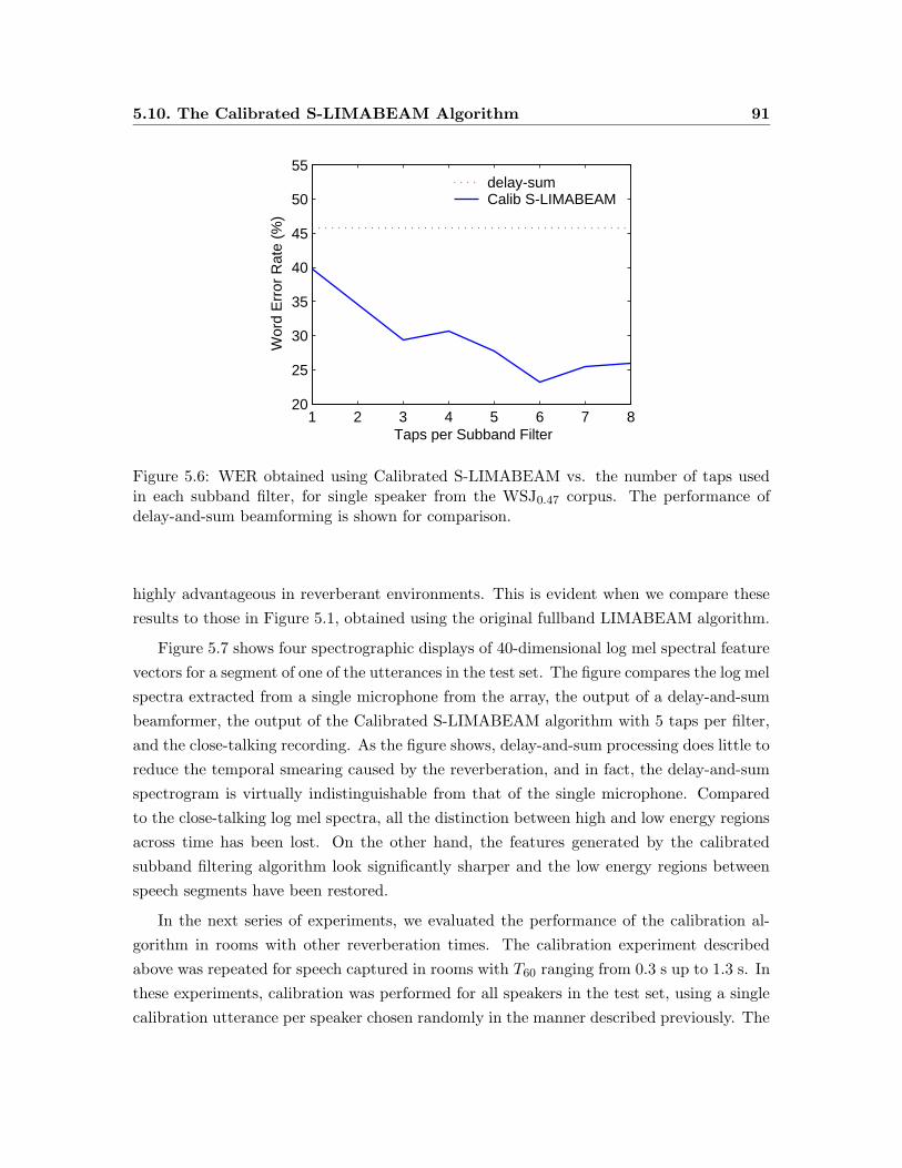
5.10. The Calibrated S-LIMABEAM Algorithm 91
1 2 3 4 5 6 7 820
25
30
35
40
45
50
55
Wor
d E
rror
Rat
e (%
)
Taps per Subband Filter
delay-sumCalib S-LIMABEAM
Figure 5.6: WER obtained using Calibrated S-LIMABEAM vs. the number of taps usedin each subband filter, for single speaker from the WSJ0.47 corpus. The performance ofdelay-and-sum beamforming is shown for comparison.
highly advantageous in reverberant environments. This is evident when we compare these
results to those in Figure 5.1, obtained using the original fullband LIMABEAM algorithm.
Figure 5.7 shows four spectrographic displays of 40-dimensional log mel spectral feature
vectors for a segment of one of the utterances in the test set. The figure compares the log mel
spectra extracted from a single microphone from the array, the output of a delay-and-sum
beamformer, the output of the Calibrated S-LIMABEAM algorithm with 5 taps per filter,
and the close-talking recording. As the figure shows, delay-and-sum processing does little to
reduce the temporal smearing caused by the reverberation, and in fact, the delay-and-sum
spectrogram is virtually indistinguishable from that of the single microphone. Compared
to the close-talking log mel spectra, all the distinction between high and low energy regions
across time has been lost. On the other hand, the features generated by the calibrated
subband filtering algorithm look significantly sharper and the low energy regions between
speech segments have been restored.
In the next series of experiments, we evaluated the performance of the calibration al-
gorithm in rooms with other reverberation times. The calibration experiment described
above was repeated for speech captured in rooms with T60 ranging from 0.3 s up to 1.3 s. In
these experiments, calibration was performed for all speakers in the test set, using a single
calibration utterance per speaker chosen randomly in the manner described previously. The
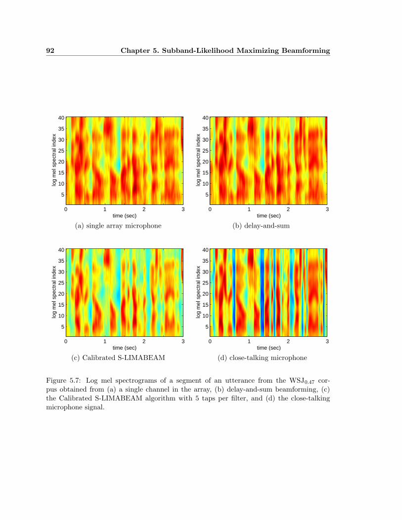
92 Chapter 5. Subband-Likelihood Maximizing Beamforming
time (sec)
log
mel
spe
ctra
l ind
ex
0 1 2 3
5
10
15
20
25
30
35
40
time (sec)
log
mel
spe
ctra
l ind
ex
0 1 2 3
5
10
15
20
25
30
35
40
(a) single array microphone (b) delay-and-sum
time (sec)
log
mel
spe
ctra
l ind
ex
0 1 2 3
5
10
15
20
25
30
35
40
time (sec)
log
mel
spe
ctra
l ind
ex
0 1 2 3
5
10
15
20
25
30
35
40
(c) Calibrated S-LIMABEAM (d) close-talking microphone
Figure 5.7: Log mel spectrograms of a segment of an utterance from the WSJ0.47 cor-pus obtained from (a) a single channel in the array, (b) delay-and-sum beamforming, (c)the Calibrated S-LIMABEAM algorithm with 5 taps per filter, and (d) the close-talkingmicrophone signal.
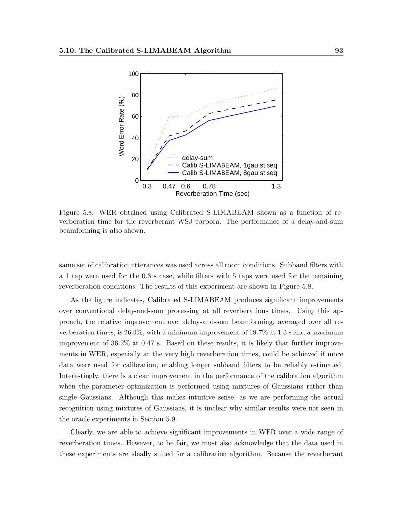
5.10. The Calibrated S-LIMABEAM Algorithm 93
0.3 0.47 0.6 0.78 1.30
20
40
60
80
100
Reverberation Time (sec)
Wor
d E
rror
Rat
e (%
)
delay-sumCalib S-LIMABEAM, 1gau st seqCalib S-LIMABEAM, 8gau st seq
Figure 5.8: WER obtained using Calibrated S-LIMABEAM shown as a function of re-verberation time for the reverberant WSJ corpora. The performance of a delay-and-sumbeamforming is also shown.
same set of calibration utterances was used across all room conditions. Subband filters with
a 1 tap were used for the 0.3 s case, while filters with 5 taps were used for the remaining
reverberation conditions. The results of this experiment are shown in Figure 5.8.
As the figure indicates, Calibrated S-LIMABEAM produces significant improvements
over conventional delay-and-sum processing at all reverberations times. Using this ap-
proach, the relative improvement over delay-and-sum beamforming, averaged over all re-
verberation times, is 26.0%, with a minimum improvement of 19.7% at 1.3 s and a maximum
improvement of 36.2% at 0.47 s. Based on these results, it is likely that further improve-
ments in WER, especially at the very high reverberation times, could be achieved if more
data were used for calibration, enabling longer subband filters to be reliably estimated.
Interestingly, there is a clear improvement in the performance of the calibration algorithm
when the parameter optimization is performed using mixtures of Gaussians rather than
single Gaussians. Although this makes intuitive sense, as we are performing the actual
recognition using mixtures of Gaussians, it is unclear why similar results were not seen in
the oracle experiments in Section 5.9.
Clearly, we are able to achieve significant improvements in WER over a wide range of
reverberation times. However, to be fair, we must also acknowledge that the data used in
these experiments are ideally suited for a calibration algorithm. Because the reverberant
94 Chapter 5. Subband-Likelihood Maximizing Beamforming
speech corpora were created by convolving clean speech with recorded room impulse re-
sponses, the distortion caused by the reverberation was exactly the same for all utterances
in the test set. This would occur if the user’s position was fixed throughout. This is a bit
unrealistic, as even a user trying to remain in place would not be perfectly still. Therefore,
it is possible that the algorithm’s performance would degrade a bit if it were applied to
data recorded by actual users. Based on our results in Chapter 4 on the CMU-8 corpus, we
expect the loss in performance to be minimal. This hypothesis, however, remains untested,
as a suitable reverberant corpus was not available.
These experiments show that the filter parameter calibration algorithm can be success-
fully incorporated into the S-LIMABEAM framework. We now turn to the unsupervised
processing case for use in situations in which the environmental conditions and/or the user’s
position may vary across utterances.
5.11 The Unsupervised S-LIMABEAM Algorithm
In Section 4.8, an algorithm was described for optimizing array processing parameters in
situations in which significant variability is expected across utterances. Recall that in this
approach, the array parameters were optimized for each utterance independently, using an
HMM state sequence derived in an unsupervised manner from a hypothesized transcription.
As in the calibration algorithm described above, the proposed subband filtering archi-
tecture can be readily incorporated into the unsupervised array processing algorithm by
simply replacing the one joint optimization over all parameters with several independent
optimizations, one for each component of the log mel spectral feature vector.
5.11.1 Experimental Results Using Unsupervised S-LIMABEAM
Unsupervised S-LIMABEAM was performed on the reverberant WSJ0.47 corpus. In all
experiments, the initial transcript used to estimate the most likely HMM state sequence
was generated using features derived from delay-and-sum processing. For optimization, the
filters were initialized to the delay-and-sum configuration after TDC was performed, as
given by Equation (5.9). Performance was evaluated using 1-, 3-, or 5-tap subband filters
and either Gaussians or mixtures of Gaussians for optimization. The results are shown in
Figure 5.9
As the figure shows, the improvement over delay-and-sum processing obtained using
unsupervised processing is only about 7% relative. Using more parameters does not improve
the performance greatly. The difference between using 1 tap and 3 taps is statistically
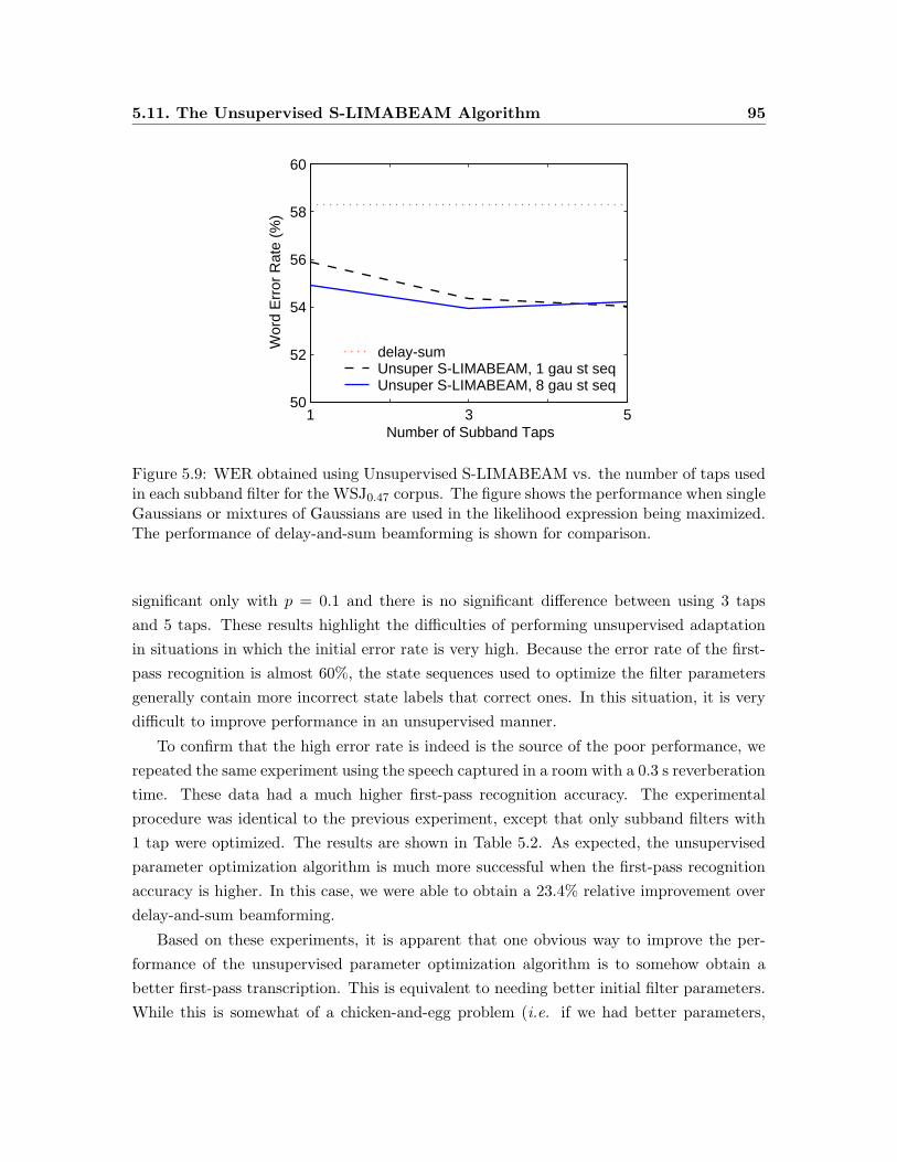
5.11. The Unsupervised S-LIMABEAM Algorithm 95
1 3 550
52
54
56
58
60
Number of Subband Taps
Wor
d E
rror
Rat
e (%
)
delay-sumUnsuper S-LIMABEAM, 1 gau st seqUnsuper S-LIMABEAM, 8 gau st seq
Figure 5.9: WER obtained using Unsupervised S-LIMABEAM vs. the number of taps usedin each subband filter for the WSJ0.47 corpus. The figure shows the performance when singleGaussians or mixtures of Gaussians are used in the likelihood expression being maximized.The performance of delay-and-sum beamforming is shown for comparison.
significant only with p = 0.1 and there is no significant difference between using 3 taps
and 5 taps. These results highlight the difficulties of performing unsupervised adaptation
in situations in which the initial error rate is very high. Because the error rate of the first-
pass recognition is almost 60%, the state sequences used to optimize the filter parameters
generally contain more incorrect state labels that correct ones. In this situation, it is very
difficult to improve performance in an unsupervised manner.
To confirm that the high error rate is indeed is the source of the poor performance, we
repeated the same experiment using the speech captured in a room with a 0.3 s reverberation
time. These data had a much higher first-pass recognition accuracy. The experimental
procedure was identical to the previous experiment, except that only subband filters with
1 tap were optimized. The results are shown in Table 5.2. As expected, the unsupervised
parameter optimization algorithm is much more successful when the first-pass recognition
accuracy is higher. In this case, we were able to obtain a 23.4% relative improvement over
delay-and-sum beamforming.
Based on these experiments, it is apparent that one obvious way to improve the per-
formance of the unsupervised parameter optimization algorithm is to somehow obtain a
better first-pass transcription. This is equivalent to needing better initial filter parameters.
While this is somewhat of a chicken-and-egg problem (i.e. if we had better parameters,
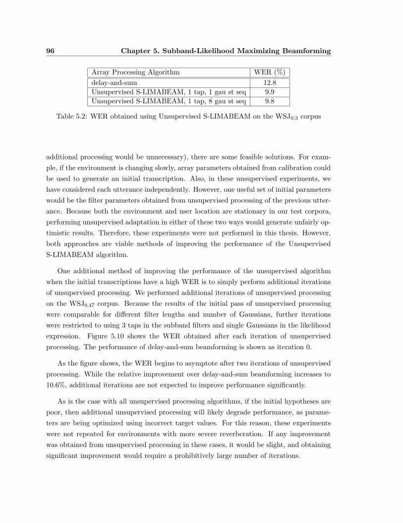
96 Chapter 5. Subband-Likelihood Maximizing Beamforming
Array Processing Algorithm WER (%)
delay-and-sum 12.8
Unsupervised S-LIMABEAM, 1 tap, 1 gau st seq 9.9
Unsupervised S-LIMABEAM, 1 tap, 8 gau st seq 9.8
Table 5.2: WER obtained using Unsupervised S-LIMABEAM on the WSJ0.3 corpus
additional processing would be unnecessary), there are some feasible solutions. For exam-
ple, if the environment is changing slowly, array parameters obtained from calibration could
be used to generate an initial transcription. Also, in these unsupervised experiments, we
have considered each utterance independently. However, one useful set of initial parameters
would be the filter parameters obtained from unsupervised processing of the previous utter-
ance. Because both the environment and user location are stationary in our test corpora,
performing unsupervised adaptation in either of these two ways would generate unfairly op-
timistic results. Therefore, these experiments were not performed in this thesis. However,
both approaches are viable methods of improving the performance of the Unsupervised
S-LIMABEAM algorithm.
One additional method of improving the performance of the unsupervised algorithm
when the initial transcriptions have a high WER is to simply perform additional iterations
of unsupervised processing. We performed additional iterations of unsupervised processing
on the WSJ0.47 corpus. Because the results of the initial pass of unsupervised processing
were comparable for different filter lengths and number of Gaussians, further iterations
were restricted to using 3 taps in the subband filters and single Gaussians in the likelihood
expression. Figure 5.10 shows the WER obtained after each iteration of unsupervised
processing. The performance of delay-and-sum beamforming is shown as iteration 0.
As the figure shows, the WER begins to asymptote after two iterations of unsupervised
processing. While the relative improvement over delay-and-sum beamforming increases to
10.6%, additional iterations are not expected to improve performance significantly.
As is the case with all unsupervised processing algorithms, if the initial hypotheses are
poor, then additional unsupervised processing will likely degrade performance, as parame-
ters are being optimized using incorrect target values. For this reason, these experiments
were not repeated for environments with more severe reverberation. If any improvement
was obtained from unsupervised processing in these cases, it would be slight, and obtaining
significant improvement would require a prohibitively large number of iterations.
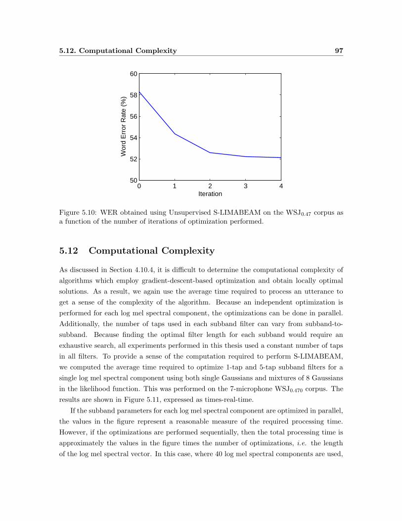
5.12. Computational Complexity 97
0 1 2 3 450
52
54
56
58
60
Iteration
Wor
d E
rror
Rat
e (%
)
Figure 5.10: WER obtained using Unsupervised S-LIMABEAM on the WSJ0.47 corpus asa function of the number of iterations of optimization performed.
5.12 Computational Complexity
As discussed in Section 4.10.4, it is difficult to determine the computational complexity of
algorithms which employ gradient-descent-based optimization and obtain locally optimal
solutions. As a result, we again use the average time required to process an utterance to
get a sense of the complexity of the algorithm. Because an independent optimization is
performed for each log mel spectral component, the optimizations can be done in parallel.
Additionally, the number of taps used in each subband filter can vary from subband-to-
subband. Because finding the optimal filter length for each subband would require an
exhaustive search, all experiments performed in this thesis used a constant number of taps
in all filters. To provide a sense of the computation required to perform S-LIMABEAM,
we computed the average time required to optimize 1-tap and 5-tap subband filters for a
single log mel spectral component using both single Gaussians and mixtures of 8 Gaussians
in the likelihood function. This was performed on the 7-microphone WSJ0.470 corpus. The
results are shown in Figure 5.11, expressed as times-real-time.
If the subband parameters for each log mel spectral component are optimized in parallel,
the values in the figure represent a reasonable measure of the required processing time.
However, if the optimizations are performed sequentially, then the total processing time is
approximately the values in the figure times the number of optimizations, i.e. the length
of the log mel spectral vector. In this case, where 40 log mel spectral components are used,
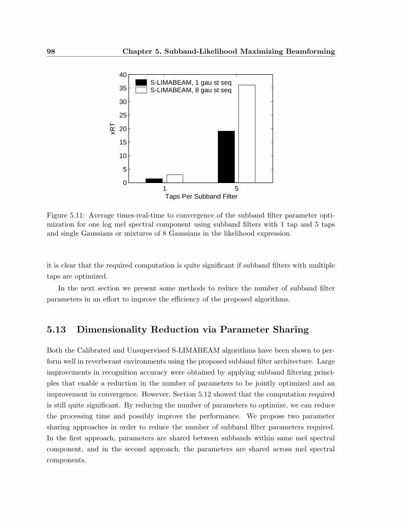
98 Chapter 5. Subband-Likelihood Maximizing Beamforming
1 50
5
10
15
20
25
30
35
40
xRT
Taps Per Subband Filter
S-LIMABEAM, 1 gau st seqS-LIMABEAM, 8 gau st seq
Figure 5.11: Average times-real-time to convergence of the subband filter parameter opti-mization for one log mel spectral component using subband filters with 1 tap and 5 tapsand single Gaussians or mixtures of 8 Gaussians in the likelihood expression.
it is clear that the required computation is quite significant if subband filters with multiple
taps are optimized.
In the next section we present some methods to reduce the number of subband filter
parameters in an effort to improve the efficiency of the proposed algorithms.
5.13 Dimensionality Reduction via Parameter Sharing
Both the Calibrated and Unsupervised S-LIMABEAM algorithms have been shown to per-
form well in reverberant environments using the proposed subband filter architecture. Large
improvements in recognition accuracy were obtained by applying subband filtering princi-
ples that enable a reduction in the number of parameters to be jointly optimized and an
improvement in convergence. However, Section 5.12 showed that the computation required
is still quite significant. By reducing the number of parameters to optimize, we can reduce
the processing time and possibly improve the performance. We propose two parameter
sharing approaches in order to reduce the number of subband filter parameters required.
In the first approach, parameters are shared between subbands within same mel spectral
component, and in the second approach, the parameters are shared across mel spectral
components.
5.13. Dimensionality Reduction via Parameter Sharing 99
5.13.1 Sharing Parameters Within Mel Spectral Components
In this approach, subband filter parameters are shared across subbands within the same
mel spectral component. Specifically, rather than estimating a separate filter for each
subband and optimizing the parameters of all subband filters jointly, only a single set of
filter parameters shared by all subbands is optimized.
By sharing parameters in this manner, the number of parameters is reduced from
M · P · (l+ − l− + 1) to simply M · P . Clearly, the reduction in the number of param-
eters is proportional to the number of subbands in a particular mel filter. For the lowest
frequency log mel spectral component, which is composed of only two subbands, the number
of parameters is reduced by 50%. For the highest frequency log mel spectral component,
composed of 23 subbands, the number of parameters required is reduced by 95.6%.
This configuration requires a small change to the formulation of the gradient for opti-
mization. The details of the derivation are given in Appendix C.
5.13.2 Sharing Parameters Across Mel Spectral Components
In the algorithms presented in this chapter, the likelihood of each component of the log mel
spectral feature vector is maximized by optimizing a set of filters applied to that component’s
constituent subbands. Because of mel filters overlap each other by 50%, this results in two
distinct filters for each subband, one for each of the mel components to which it contributes.†
This approach is well-suited to our assumption that the components of the log mel spectral
vector are independent. Specifically, by using two different filters for the same subband,
the likelihood of each of the log mel spectral components can be maximized independently,
without affecting the likelihood of the other components.
However, adjacent mel components are actually highly correlated. The mel spectrum is
derived from the energy in overlapping frequency bands such that subbands in the right half
(higher frequencies) of one mel triangle are also in the left half (lower frequencies) of the
next mel triangle. It is reasonable to expect, then, that for each subband, the two filters,
optimized for adjacent mel components, will be similar. Therefore, we propose to reduce
the number of total parameters estimated by optimizing a single filter for each subband,
which will be used to generate both mel components.
The optimal way to estimate such a filter would be to jointly maximize the likelihood
of both log mel spectral components. However, because of the overlap in subbands, jointly
maximizing the likelihood of two components cannot be done without maximizing the likeli-
†In practice, because of the quantization in frequency caused by the DFT, the overlap between adjacentmel filters can vary and as a result, not all subbands are necessarily used by two mel filters.
100 Chapter 5. Subband-Likelihood Maximizing Beamforming
hood jointly over all mel components. This requires a joint optimization over all subbands,
which defeats the purpose of subband processing entirely.
Instead, we assume that for the subbands included in two mel components, the filter
parameters that maximize the likelihood of one mel component also maximize the likelihood
of the next component. In other words, the subband filter optimized when its corresponding
subband is in the right half of one mel filter is also optimal for that same subband when
it is in the left half of the next mel filter. Thus the components of the log mel spectral
vector are optimized in succession. For each component, the filters used to optimize the
previous component are copied and assumed fixed, and only the filters for new subbands
(which will in turn be used for the next component) are optimized. The changes to the
gradient derivation required to share parameters in this manner are described in Appendix
C.
5.13.3 Experimental Results Using Parameter Sharing
Experiments were performed using these two methods of parameter reduction in order to
compare their performance to the original subband filtering architecture. We will evaluate
the methods both in terms of speech recognition accuracy and computational efficiency. In
the first experiment, the Unsupervised S-LIMABEAM algorithm was applied to the WSJ0.3
corpus using 1 tap per subband filter. In the second experiment, the array calibration
algorithm was applied to the WSJ0.47 corpus, using 5 taps per subband filter. In these
experiments, we computed both the speech recognition accuracy and the average time to
convergence of the two parameter sharing configurations, relative to the original subband
architecture. These values were obtained as follows. Each experiment was run on the same
computer and the average time to convergence was computed over all utterances for each
configuration. The values were then normalized by the average time to convergence of the
original subband algorithm. This measure provides some sense of the computational savings
afforded by these parameter sharing methods and the potential performance versus time
trade-offs. The results of these experiments are summarized in Table 5.3.
As the data in the table shows, these parameter sharing methods provide a significant
reduction in computation for a small reduction in performance.
5.14 S-LIMABEAM in Environments with Low Reverberation
In this chapter we have proposed a subband filtering approach to the LIMABEAM frame-
work presented in the previous chapter. The algorithms presented in this chapter were
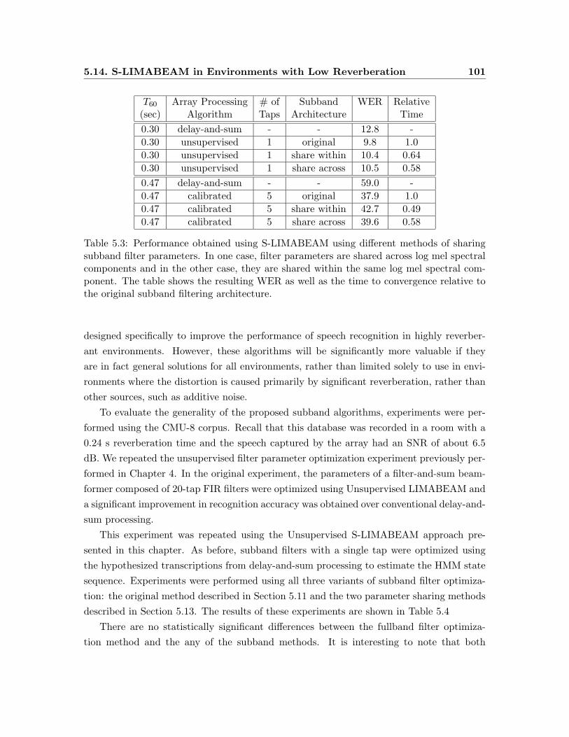
5.14. S-LIMABEAM in Environments with Low Reverberation 101
T60 Array Processing # of Subband WER Relative(sec) Algorithm Taps Architecture Time
0.30 delay-and-sum - - 12.8 -
0.30 unsupervised 1 original 9.8 1.0
0.30 unsupervised 1 share within 10.4 0.64
0.30 unsupervised 1 share across 10.5 0.58
0.47 delay-and-sum - - 59.0 -
0.47 calibrated 5 original 37.9 1.0
0.47 calibrated 5 share within 42.7 0.49
0.47 calibrated 5 share across 39.6 0.58
Table 5.3: Performance obtained using S-LIMABEAM using different methods of sharingsubband filter parameters. In one case, filter parameters are shared across log mel spectralcomponents and in the other case, they are shared within the same log mel spectral com-ponent. The table shows the resulting WER as well as the time to convergence relative tothe original subband filtering architecture.
designed specifically to improve the performance of speech recognition in highly reverber-
ant environments. However, these algorithms will be significantly more valuable if they
are in fact general solutions for all environments, rather than limited solely to use in envi-
ronments where the distortion is caused primarily by significant reverberation, rather than
other sources, such as additive noise.
To evaluate the generality of the proposed subband algorithms, experiments were per-
formed using the CMU-8 corpus. Recall that this database was recorded in a room with a
0.24 s reverberation time and the speech captured by the array had an SNR of about 6.5
dB. We repeated the unsupervised filter parameter optimization experiment previously per-
formed in Chapter 4. In the original experiment, the parameters of a filter-and-sum beam-
former composed of 20-tap FIR filters were optimized using Unsupervised LIMABEAM and
a significant improvement in recognition accuracy was obtained over conventional delay-and-
sum processing.
This experiment was repeated using the Unsupervised S-LIMABEAM approach pre-
sented in this chapter. As before, subband filters with a single tap were optimized using
the hypothesized transcriptions from delay-and-sum processing to estimate the HMM state
sequence. Experiments were performed using all three variants of subband filter optimiza-
tion: the original method described in Section 5.11 and the two parameter sharing methods
described in Section 5.13. The results of these experiments are shown in Table 5.4
There are no statistically significant differences between the fullband filter optimiza-
tion method and the any of the subband methods. It is interesting to note that both
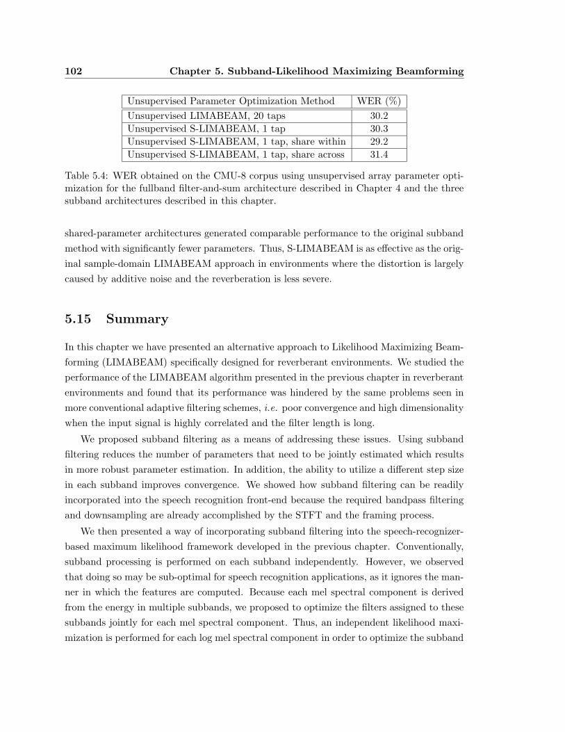
102 Chapter 5. Subband-Likelihood Maximizing Beamforming
Unsupervised Parameter Optimization Method WER (%)
Unsupervised LIMABEAM, 20 taps 30.2
Unsupervised S-LIMABEAM, 1 tap 30.3
Unsupervised S-LIMABEAM, 1 tap, share within 29.2
Unsupervised S-LIMABEAM, 1 tap, share across 31.4
Table 5.4: WER obtained on the CMU-8 corpus using unsupervised array parameter opti-mization for the fullband filter-and-sum architecture described in Chapter 4 and the threesubband architectures described in this chapter.
shared-parameter architectures generated comparable performance to the original subband
method with significantly fewer parameters. Thus, S-LIMABEAM is as effective as the orig-
inal sample-domain LIMABEAM approach in environments where the distortion is largely
caused by additive noise and the reverberation is less severe.
5.15 Summary
In this chapter we have presented an alternative approach to Likelihood Maximizing Beam-
forming (LIMABEAM) specifically designed for reverberant environments. We studied the
performance of the LIMABEAM algorithm presented in the previous chapter in reverberant
environments and found that its performance was hindered by the same problems seen in
more conventional adaptive filtering schemes, i.e. poor convergence and high dimensionality
when the input signal is highly correlated and the filter length is long.
We proposed subband filtering as a means of addressing these issues. Using subband
filtering reduces the number of parameters that need to be jointly estimated which results
in more robust parameter estimation. In addition, the ability to utilize a different step size
in each subband improves convergence. We showed how subband filtering can be readily
incorporated into the speech recognition front-end because the required bandpass filtering
and downsampling are already accomplished by the STFT and the framing process.
We then presented a way of incorporating subband filtering into the speech-recognizer-
based maximum likelihood framework developed in the previous chapter. Conventionally,
subband processing is performed on each subband independently. However, we observed
that doing so may be sub-optimal for speech recognition applications, as it ignores the man-
ner in which the features are computed. Because each mel spectral component is derived
from the energy in multiple subbands, we proposed to optimize the filters assigned to these
subbands jointly for each mel spectral component. Thus, an independent likelihood maxi-
mization is performed for each log mel spectral component in order to optimize the subband
5.15. Summary 103
filter parameters required to compute that component. In short, a single joint optimiza-
tion over all filter parameters for all microphones is replaced by multiple optimizations of
select groups of subband filter parameters. We refer to this method as Subband-Likelihood
Maximizing Beamforming (S-LIMABEAM).
This feature-based subband filter optimization scheme was then incorporated into the
calibration and unsupervised array processing algorithms developed in the previous chapter.
Using Calibrated S-LIMABEAM, we obtained significant improvements in recognition ac-
curacy in environments with reverberation times up to 1.3 s. Predictably, the performance
of Unsupervised S-LIMABEAM was dependent on the accuracy of the estimated transcrip-
tions. At moderate reverberation levels, we were able to obtain substantial improvements
in recognition accuracy. However, at higher levels of reverberation, the estimated transcrip-
tions had error rates upwards of 60% and as a result, the improvements were smaller. We
suggested some methods of obtaining better initial transcriptions in order to improve the
performance in such situations.
We then examined the computational complexity of the algorithm and showed that al-
though we are able to obtain substantial improvements in recognition accuracy, they come
at a significant computational cost. However, we noted that there are several places where
the efficiency of the algorithm could be improved. In an effort to reduce the computational
complexity of the subband optimization scheme, we presented two methods of sharing filter
parameters across subbands. In one method, filters are shared across mel spectral com-
ponents and in the other, parameters are shared within mel spectral components. These
methods reduced the time to convergence by 40− 50% with minimal degradation in perfor-
mance.
Finally, we examined the performance of S-LIMABEAM on data with less reverberation
and significant additive noise. We obtained the same performance as that achieved by the
original fullband LIMABEAM algorithm, showing that the proposed method is not specific
to reverberant environments and can be applied in all situations.
In the next chapter we apply both LIMABEAM and S-LIMABEAM to other multi-
microphone applications in order to highlight additional benefits of using a purely data-
driven approach to microphone array processing.

Chapter 6
LIMABEAM in Other
Multi-Microphone Environments
6.1 Introduction
In Chapters 4 and 5, algorithms were presented for improving speech recognition perfor-
mance in environments in which an array of microphones is used to capture the incoming
speech signals. In these algorithms, the array processing parameters are manipulated in
such a way so as to maximize the likelihood of the sequence of features generated from the
array output signal for what is believed to be the correct recognizer hypothesis. This is
done is a purely data-driven manner, using the statistical models of the recognition system
to derive the target parameters of the likelihood function. As mentioned previously, these
algorithms differ from previous methods in that the optimization is performed in the feature
space used by the recognizer, rather that at the signal level using criteria such as SNR or
the error compared to a desired waveform.
There is another key difference between the proposed method of processing and many
other array processing algorithms. Many array processing methods require that the micro-
phones to be configured according to some specific geometry, known a priori . For example,
the harmonic-nested array uses a logarithmic spacing of the microphones to obtain a desired
beampattern (Flanagan et al., 1991). Superdirective beamformers (Cox et al., 1987) require
the microphones to be arranged in an endfire arrangement in order to obtain optimal gain
in the look direction. Some algorithms actually optimize microphone placement or array
geometry, e.g. (Rabinkin et al., 1997; Kajala & Hamalainen, 1999). In contrast, the algo-
rithms in this thesis place no such constraints on the array geometry. Because the processing
is data-driven, no inherent assumption of array geometry is made. The algorithm merely
105
106 Chapter 6. LIMABEAM in Other Multi-Microphone Environments
processes the input signals it receives. Because there are no assumptions about geometry,
we can apply these algorithms to any multi-channel scenario, even if the arrangement of
microphones varies widely or is sub-optimal from a traditional array processing point of
view. Furthermore, regardless of the configuration of the microphones, no changes to the
algorithms are necessary as all processing occurs in a data-driven manner.
In this chapter, two multi-microphone configurations are considered. First, the use of
multiple microphones placed on a Personal Digital Assistant (PDA) is examined. In this
case, the microphones are placed in a two-dimensional geometry at the four corners of the
device. In the second case, a meeting room environment is studied in which four microphones
are placed along the center of a long conference room table. From a traditional array
processing point of view, the arrangement used is highly-suboptimal, but we can nevertheless
attempt to process the signals with our algorithms. The experiments performed in this
section show that the algorithms presented in this thesis are capable of good performance
with only a small number of channels without any specific dependence on the geometric
configuration of the microphones.
6.2 Multi-microphone Speech Recognition on a PDA
The use of PDAs has dramatically increased over the last several years. The interface of
most PDAs is centered around the use of a pen-like device called a stylus. Clicking a mouse
button is replaced by tapping the stylus on the screen. Text is entered by writing on the
screen using the stylus, usually in some specific pre-defined fashion. This is suitable for
short entries such as phone numbers but is inefficient for entering longer texts. Speech has
been viewed as a viable modality for these interactions. While a good idea in principle,
this is difficult in practice for several reasons. The memory size of a PDA is limited, so
getting a recognizer to fit within the computational footprint of a PDA is a difficult task.
Some researchers have avoided this problem by using an architecture in which the PDA
is a client that communicates with a recognition server hosted on another larger machine,
e.g. (Deng et al., 2002). Another significant hurdle is actually capturing the speech signal.
Most PDAs have only a single low-cost microphone paired with a low-quality audio CODEC
(COder/DECoder), which makes high quality sound capture difficult.
One potential method of improving the quality of the audio capture is to equip PDAs
with multiple low-cost microphones and utilize array processing technology. To this end,
we evaluated the performance of the algorithms in this thesis for PDA applications.
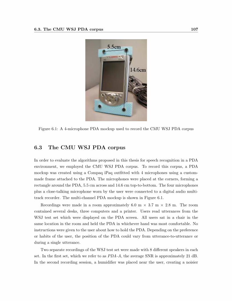
6.3. The CMU WSJ PDA corpus 107
Figure 6.1: A 4-microphone PDA mockup used to record the CMU WSJ PDA corpus
6.3 The CMU WSJ PDA corpus
In order to evaluate the algorithms proposed in this thesis for speech recognition in a PDA
environment, we employed the CMU WSJ PDA corpus. To record this corpus, a PDA
mockup was created using a Compaq iPaq outfitted with 4 microphones using a custom-
made frame attached to the PDA. The microphones were placed at the corners, forming a
rectangle around the PDA, 5.5 cm across and 14.6 cm top-to-bottom. The four microphones
plus a close-talking microphone worn by the user were connected to a digital audio multi-
track recorder. The multi-channel PDA mockup is shown in Figure 6.1.
Recordings were made in a room approximately 6.0 m × 3.7 m × 2.8 m. The room
contained several desks, three computers and a printer. Users read utterances from the
WSJ test set which were displayed on the PDA screen. All users sat in a chair in the
same location in the room and held the PDA in whichever hand was most comfortable. No
instructions were given to the user about how to hold the PDA. Depending on the preference
or habits of the user, the position of the PDA could vary from utterance-to-utterance or
during a single utterance.
Two separate recordings of the WSJ test set were made with 8 different speakers in each
set. In the first set, which we refer to as PDA-A, the average SNR is approximately 21 dB.
In the second recording session, a humidifier was placed near the user, creating a noisier
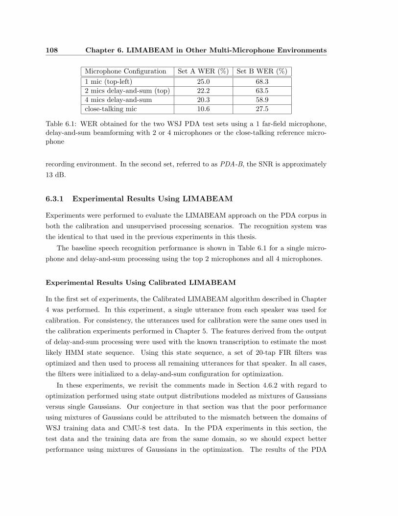
108 Chapter 6. LIMABEAM in Other Multi-Microphone Environments
Microphone Configuration Set A WER (%) Set B WER (%)
1 mic (top-left) 25.0 68.3
2 mics delay-and-sum (top) 22.2 63.5
4 mics delay-and-sum 20.3 58.9
close-talking mic 10.6 27.5
Table 6.1: WER obtained for the two WSJ PDA test sets using a 1 far-field microphone,delay-and-sum beamforming with 2 or 4 microphones or the close-talking reference micro-phone
recording environment. In the second set, referred to as PDA-B, the SNR is approximately
13 dB.
6.3.1 Experimental Results Using LIMABEAM
Experiments were performed to evaluate the LIMABEAM approach on the PDA corpus in
both the calibration and unsupervised processing scenarios. The recognition system was
the identical to that used in the previous experiments in this thesis.
The baseline speech recognition performance is shown in Table 6.1 for a single micro-
phone and delay-and-sum processing using the top 2 microphones and all 4 microphones.
Experimental Results Using Calibrated LIMABEAM
In the first set of experiments, the Calibrated LIMABEAM algorithm described in Chapter
4 was performed. In this experiment, a single utterance from each speaker was used for
calibration. For consistency, the utterances used for calibration were the same ones used in
the calibration experiments performed in Chapter 5. The features derived from the output
of delay-and-sum processing were used with the known transcription to estimate the most
likely HMM state sequence. Using this state sequence, a set of 20-tap FIR filters was
optimized and then used to process all remaining utterances for that speaker. In all cases,
the filters were initialized to a delay-and-sum configuration for optimization.
In these experiments, we revisit the comments made in Section 4.6.2 with regard to
optimization performed using state output distributions modeled as mixtures of Gaussians
versus single Gaussians. Our conjecture in that section was that the poor performance
using mixtures of Gaussians could be attributed to the mismatch between the domains of
WSJ training data and CMU-8 test data. In the PDA experiments in this section, the
test data and the training data are from the same domain, so we should expect better
performance using mixtures of Gaussians in the optimization. The results of the PDA
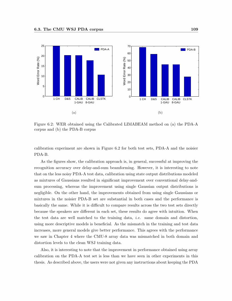
6.3. The CMU WSJ PDA corpus 109
1 CH D&S CALIB CALIB CLSTK0
5
10
15
20
25
Wor
d E
rror
Rat
e (%
)
1-GAU 8-GAU
PDA-A
(a)
1 CH D&S CALIB CALIB CLSTK0
10
20
30
40
50
60
70
Wor
d E
rror
Rat
e (%
)
1-GAU 8-GAU
PDA-B
(b)
Figure 6.2: WER obtained using the Calibrated LIMABEAM method on (a) the PDA-Acorpus and (b) the PDA-B corpus
calibration experiment are shown in Figure 6.2 for both test sets, PDA-A and the noisier
PDA-B.
As the figures show, the calibration approach is, in general, successful at improving the
recognition accuracy over delay-and-sum beamforming. However, it is interesting to note
that on the less noisy PDA-A test data, calibration using state output distributions modeled
as mixtures of Gaussians resulted in significant improvement over conventional delay-and-
sum processing, whereas the improvement using single Gaussian output distributions is
negligible. On the other hand, the improvements obtained from using single Gaussians or
mixtures in the noisier PDA-B set are substantial in both cases and the performance is
basically the same. While it is difficult to compare results across the two test sets directly
because the speakers are different in each set, these results do agree with intuition. When
the test data are well matched to the training data, i.e. same domain and distortion,
using more descriptive models is beneficial. As the mismatch in the training and test data
increases, more general models give better performance. This agrees with the performance
we saw in Chapter 4 where the CMU-8 array data was mismatched in both domain and
distortion levels to the clean WSJ training data.
Also, it is interesting to note that the improvement in performance obtained using array
calibration on the PDA-A test set is less than we have seen in other experiments in this
thesis. As described above, the users were not given any instructions about keeping the PDA
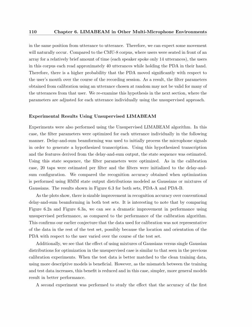
110 Chapter 6. LIMABEAM in Other Multi-Microphone Environments
in the same position from utterance to utterance. Therefore, we can expect some movement
will naturally occur. Compared to the CMU-8 corpus, where users were seated in front of an
array for a relatively brief amount of time (each speaker spoke only 14 utterances), the users
in this corpus each read approximately 40 utterances while holding the PDA in their hand.
Therefore, there is a higher probability that the PDA moved significantly with respect to
the user’s mouth over the course of the recording session. As a result, the filter parameters
obtained from calibration using an utterance chosen at random may not be valid for many of
the utterances from that user. We re-examine this hypothesis in the next section, where the
parameters are adjusted for each utterance individually using the unsupervised approach.
Experimental Results Using Unsupervised LIMABEAM
Experiments were also performed using the Unsupervised LIMABEAM algorithm. In this
case, the filter parameters were optimized for each utterance individually in the following
manner. Delay-and-sum beamforming was used to initially process the microphone signals
in order to generate a hypothesized transcription. Using this hypothesized transcription
and the features derived from the delay-and-sum output, the state sequence was estimated.
Using this state sequence, the filter parameters were optimized. As in the calibration
case, 20 taps were estimated per filter and the filters were initialized to the delay-and-
sum configuration. We compared the recognition accuracy obtained when optimization
is performed using HMM state output distributions modeled as Gaussians or mixtures of
Gaussians. The results shown in Figure 6.3 for both sets, PDA-A and PDA-B.
As the plots show, there is sizable improvement in recognition accuracy over conventional
delay-and-sum beamforming in both test sets. It is interesting to note that by comparing
Figure 6.2a and Figure 6.3a, we can see a dramatic improvement in performance using
unsupervised performance, as compared to the performance of the calibration algorithm.
This confirms our earlier conjecture that the data used for calibration was not representative
of the data in the rest of the test set, possibly because the location and orientation of the
PDA with respect to the user varied over the course of the test set.
Additionally, we see that the effect of using mixtures of Gaussians versus single Gaussian
distributions for optimization in the unsupervised case is similar to that seen in the previous
calibration experiments. When the test data is better matched to the clean training data,
using more descriptive models is beneficial. However, as the mismatch between the training
and test data increases, this benefit is reduced and in this case, simpler, more general models
result in better performance.
A second experiment was performed to study the effect that the accuracy of the first
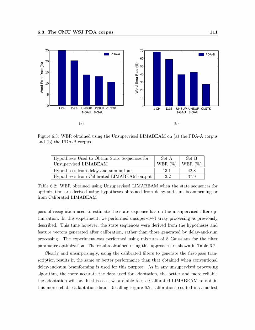
6.3. The CMU WSJ PDA corpus 111
1 CH D&S UNSUP UNSUP CLSTK0
5
10
15
20
25
Wor
d E
rror
Rat
e (%
)
1-GAU 8-GAU
PDA-A
(a)
1 CH D&S UNSUP UNSUP CLSTK0
10
20
30
40
50
60
70
Wor
d E
rror
Rat
e (%
)
1-GAU 8-GAU
PDA-B
(b)
Figure 6.3: WER obtained using the Unsupervised LIMABEAM on (a) the PDA-A corpusand (b) the PDA-B corpus
Hypotheses Used to Obtain State Sequences for Set A Set BUnsupervised LIMABEAM WER (%) WER (%)
Hypotheses from delay-and-sum output 13.1 42.8
Hypotheses from Calibrated LIMABEAM output 13.2 37.9
Table 6.2: WER obtained using Unsupervised LIMABEAM when the state sequences foroptimization are derived using hypotheses obtained from delay-and-sum beamforming orfrom Calibrated LIMABEAM
pass of recognition used to estimate the state sequence has on the unsupervised filter op-
timization. In this experiment, we performed unsupervised array processing as previously
described. This time however, the state sequences were derived from the hypotheses and
feature vectors generated after calibration, rather than those generated by delay-and-sum
processing. The experiment was performed using mixtures of 8 Gaussians for the filter
parameter optimization. The results obtained using this approach are shown in Table 6.2.
Clearly and unsurprisingly, using the calibrated filters to generate the first-pass tran-
scription results in the same or better performance than that obtained when conventional
delay-and-sum beamforming is used for this purpose. As in any unsupervised processing
algorithm, the more accurate the data used for adaptation, the better and more reliable
the adaptation will be. In this case, we are able to use Calibrated LIMABEAM to obtain
this more reliable adaptation data. Recalling Figure 6.2, calibration resulted in a modest
112 Chapter 6. LIMABEAM in Other Multi-Microphone Environments
improvement over delay-and-sum processing for the PDA-A data set while the improvement
for the PDA-B set was far greater. As a result, using the transcriptions from calibration
for Unsupervised LIMABEAM resulted in the same performance on PDA-A (the difference
between the two results is not statistically significant) and resulted in an additional 8.3%
relative improvement over delay-and-sum processing on PDA-B.
6.3.2 Summary of Experimental Results
In this section, we examined the application of LIMABEAM to a PDA with 4-microphones
for audio capture, rather than a single microphone. Experiments were performed in which
20-tap filters were optimized in the proposed LIMABEAM framework using both the
calibration and the unsupervised approaches described in Chapter 4. Using Calibrated
LIMABEAM, an average relative improvement of 18.8% over delay-and-sum beamforming
over both PDA test sets was obtained. Using Unsupervised LIMABEAM, an average rela-
tive improvement of 31.4% over delay-and-sum beamforming was obtained. Finally, when
these two methods were combined and the unsupervised adaptation was performed using
transcriptions generated after calibration, the relative improvement increased to 35.3%.
The Generalized Sidelobe Canceller (GSC) algorithm with parameter adaptation during
the non-speech regions only was also attempted on the PDA data. The performance was
significantly worse than simple delay-and-sum beamforming and therefore the results were
not reported here.
6.4 Meeting Transcription with Multiple Tabletop
Microphones
Recently, improvements in both speech recognition and audio indexing technologies have
led to increased interest in the automatic transcription and indexing of meetings. In such
a scenario, one or more microphones are used to capture the dialog during a meeting. This
audio could then be processed and a transcription of the meeting obtained automatically
via speech recognition. In addition, the transcriptions plus additional information extracted
from the audio signal(s) could then be used to generate higher level descriptions of the
meeting, such as the speaker turns, topic shift, etc. This is a very challenging problem
receiving attention from several sites, e.g. (Morgan et al., 2003; Waibel et al., 2001; Cutler
et al., 2002). In some meeting room environments, users wear either close-talking headset
microphones or lapel microphones. The use of such microphones creates a cumbersome and
unnatural experience for the participants. Ideally, the audio would be captured by one or
6.5. The ICSI Meeting Recorder Corpus 113
more farfield microphones.
Some sites have created rooms in which an extremely large number of microphones
(> 100) are distributed around the room, e.g. (Silverman et al., 1996). While such ap-
proaches can produce significant speech enhancement, they are significantly more costly
than microphone arrays with a smaller number of microphones and require much more
hardware to process such a large number of data streams. In addition, these solutions are
highly non-portable, a significant drawback when one considers the large number of con-
ference rooms in a typical company or university. Installing such an array in each of these
rooms would be prohibitively expensive.
A more conventional solution would utilize one or more arrays with a smaller number of
microphones located on the table, walls or ceiling. A more appealing approach is to simply
place a few microphones on the table either in a fixed geometry, or more interestingly, in
some reasonable, though unspecified configuration, e.g. roughly equally distributed along
the table. This latter scenario has the dual advantage of being an inexpensive and highly
portable method of audio capture. One could imagine arriving to any room for a meeting,
putting some number of microphones along the table, connecting them to a laptop com-
puter, and recording the meeting directly to disk. In such a scenario, the array geometry
is unknown a priori and as such, algorithms requiring a particular geometry will fail. Fur-
thermore, the microphone configuration could be highly sub-optimal for conventional array
processing approaches. In spite of these challenges, this is the scenario we explore in the
next section.
6.5 The ICSI Meeting Recorder Corpus
Researchers at the International Computer Science Institute (ICSI) have collected a corpus
of meeting data by recording their own meetings over the last three years. The audio
in each meeting was captured by a close-talking microphone worn by each user, as well
as four PZM microphones placed along the conference room table and two microphones
embedded in a wooden PDA mockup. The meeting room environment is shown in Figure
6.4. The locations of the four PZM microphones are indicated by the black circles. The
majority of the speech during these meetings was spontaneous, multi-party conversation
typical of meetings. In addition, during each meeting, each participant read several strings
of connected digits. The speech recorded during each meeting was transcribed by hand.
More details about this corpus can be found in (Janin et al., 2003).
We are interested in determining if the methods presented in this thesis can be applied
to this data in order to improve the speech recognition accuracy when only the four tabletop
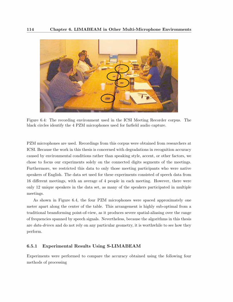
114 Chapter 6. LIMABEAM in Other Multi-Microphone Environments
Figure 6.4: The recording environment used in the ICSI Meeting Recorder corpus. Theblack circles identify the 4 PZM microphones used for farfield audio capture.
PZM microphones are used. Recordings from this corpus were obtained from researchers at
ICSI. Because the work in this thesis is concerned with degradations in recognition accuracy
caused by environmental conditions rather than speaking style, accent, or other factors, we
chose to focus our experiments solely on the connected digits segments of the meetings.
Furthermore, we restricted this data to only those meeting participants who were native
speakers of English. The data set used for these experiments consisted of speech data from
16 different meetings, with an average of 4 people in each meeting. However, there were
only 12 unique speakers in the data set, as many of the speakers participated in multiple
meetings.
As shown in Figure 6.4, the four PZM microphones were spaced approximately one
meter apart along the center of the table. This arrangement is highly sub-optimal from a
traditional beamforming point-of-view, as it produces severe spatial-aliasing over the range
of frequencies spanned by speech signals. Nevertheless, because the algorithms in this thesis
are data-driven and do not rely on any particular geometry, it is worthwhile to see how they
perform.
6.5.1 Experimental Results Using S-LIMABEAM
Experiments were performed to compare the accuracy obtained using the following four
methods of processing
6.6. Summary 115
• Using one PZM microphone for all speakers
• Selecting the PZM microphone with the highest SNR for each utterance, i.e. thesingle best microphone
• Delay-and-sum processing
• Unsupervised S-LIMABEAM, as described in Chapter 5
In order to choose the microphone with the highest SNR for the second method, the
SNR of each of the four microphones was estimated for every utterance using SNR estima-
tion software from NIST (Pallett et al., 1996). For each utterance, the microphone with the
highest SNR was used for recognition. For both delay-and-sum processing and the subband
calibration method, Time-Delay Compensation was performed for using the PHAT algo-
rithm, as in all previous experiments. The range of acceptable delay values was increased
to account for the wide microphone spacing.
Unsupervised S-LIMABEAM was performed as follows. For all utterances, features
derived from delay-and-sum processing were used to generate an initial transcription. Based
on this transcription, the most likely HMM state sequence was estimated and used to
optimize subband filters with a single tap.
The results of this experiment are shown in Figure 6.5. As the figure shows, simply
selecting the one farfield microphone with the highest SNR (presumably the one closest to
the user speaking) results in a relative improvement in WER of about 70% over the use of a
single farfield microphone for all speakers. Although the microphone arrangement is highly
sub-optimal, delay-and-sum processing is able to improve performance further still. Yet,
even with this atypical multi-microphone configuration, the best results are obtained using
Unsupervised S-LIMABEAM, which provides a 21.9% relative improvement over delay-and-
sum processing.
6.6 Summary
In this chapter, we have examined the application of the array processing algorithms pre-
sented in this thesis to other multi-microphone applications. Specifically, we studied speech
recognition on a PDA and automatic meeting transcription using multiple tabletop micro-
phones. Because LIMABEAM is a purely data-driven approach, there are no constraints on
the microphone array geometry and a priori knowledge is not required by the algorithms.
Any signals received from multiple microphones can be processed without any modification
to the algorithms.
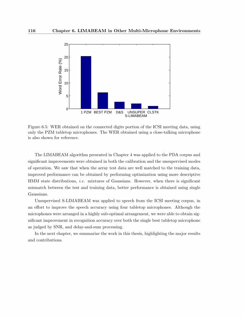
116 Chapter 6. LIMABEAM in Other Multi-Microphone Environments
1 PZM BEST PZM D&S UNSUPER CLSTK0
5
10
15
20
25
Wor
d E
rror
Rat
e (%
)
S-LIMABEAM
Figure 6.5: WER obtained on the connected digits portion of the ICSI meeting data, usingonly the PZM tabletop microphones. The WER obtained using a close-talking microphoneis also shown for reference.
The LIMABEAM algorithm presented in Chapter 4 was applied to the PDA corpus and
significant improvements were obtained in both the calibration and the unsupervised modes
of operation. We saw that when the array test data are well matched to the training data,
improved performance can be obtained by performing optimization using more descriptive
HMM state distributions, i.e. mixtures of Gaussians. However, when there is significant
mismatch between the test and training data, better performance is obtained using single
Gaussians.
Unsupervised S-LIMABEAM was applied to speech from the ICSI meeting corpus, in
an effort to improve the speech accuracy using four tabletop microphones. Although the
microphones were arranged in a highly sub-optimal arrangement, we were able to obtain sig-
nificant improvement in recognition accuracy over both the single best tabletop microphone
as judged by SNR, and delay-and-sum processing.
In the next chapter, we summarize the work in this thesis, highlighting the major results
and contributions.
Chapter 7
Summary and Conclusions
7.1 Introduction
In this thesis we have sought to improve speech recognition accuracy in environments where
a close-talking microphone is not available and the speech is captured by an array of mi-
crophones located some distance from the user. As the distance between the user and the
microphones increases, the speech signal is increasingly distorted by the effects of addi-
tive noise and reverberation, which in turn, degrade the performance of speech recognition
systems.
Conventional microphone array processing algorithms manipulate the signals received
by the array according to various waveform-level objective criteria in order to generate
an enhanced output signal. In previous approaches to speech recognition with microphone
arrays, one of these methods is used to pre-process the received signals in order to generate a
higher quality single-channel output waveform for recognition. Such an approach to speech
recognition incorrectly assumes that generating an enhanced waveform will necessarily result
in improved recognition accuracy. By making this assumption, the manner in which a
speech recognizer operates is ignored. As a result, sophisticated microphone array processing
algorithms capable of generating high-quality output waveforms do not produce significant
improvements in speech recognition accuracy over far simpler methods, such as delay-and-
sum beamforming.
The work presented in this thesis takes a signficantly different approach by considering
the microphone array processor and the speech recognition system as components of a single
system. In this approach, the objective of the array processor is no longer to generate a
higher-quality output waveform. Rather, the array processor and speech recognizer, operat-
ing in tandem, share the common objective of improved speech recognition accuracy. This
117
118 Chapter 7. Summary and Conclusions
objective is met by incorporating into the array processing scheme both 1) how speech is
processed by the recognizer, i.e. the feature extraction process, and 2) how these features
are used to hypothesize the words spoken, i.e. according to a maximum likelihood criterion
using statistical models of speech sound units. By creating such a framework, we are able
to “close the loop” between the array processor and speech recognizer. This allows infor-
mation from the recognition system to be used to optimize the array processing parameters
specifically for improved recognition accuracy.
In the remainder of this chapter, we summarize the findings and contributions of this
thesis, present some remaining open questions about the work described in this thesis, and
suggest some directions for further research.
7.2 Summary of Findings and Contributions of This Thesis
In this thesis we have developed a filter-and-sum array processing algorithm called Likeli-
hood Maximizing Beamforming (LIMABEAM) in which the filter parameters are optimized
in a data-driven fashion using the statistical models of a speech recognition system. We
formulate the optimization of the filters parameters as a maximum likelihood parameter
estimation problem. We showed how the optimal values for the parameters are those which
maximize the likelihood of the correct transcription of the given utterance. Via this likeli-
hood function, we explicitly make the connection between the array processing parameters,
the feature extraction process, and the statistical models of the recognizer. Optimizing the
parameters in this manner ensures that signal components important for recognition are
emphasized without undue emphasis on less important components.
Using this framework, we developed two algorithms to optimize the parameters of a
filter-and-sum beamformer. In the first method, called Calibrated LIMABEAM, an enroll-
ment utterance with a known transcription is spoken by the user and used to optimize the
filter parameters (Seltzer & Raj, 2001). These filter parameters are then used to process fu-
ture utterances. This algorithm is appropriate for situations in which the environment and
the user’s position do not vary significantly over time, such as in a car or in front of a desk-
top computer. For time-varying environments, we developed an algorithm for optimizing
the filter parameters in an unsupervised manner. In Unsupervised LIMABEAM, the opti-
mization is performed on each utterance independently using a hypothesized transcription
obtained from an initial pass of recognition (Seltzer et al., 2002).
Both of these methods were able to obtain significant improvements in recognition ac-
curacy in environments with moderate reverberation over a wide range of noise levels.
However, we found that if too little speech data were used for the optimization, the im-
7.2. Summary of Findings and Contributions of This Thesis 119
provements in recognition accuracy were small. In the calibration case, too little data
resulted in overfitting and unreliable parameter estimation, while in the unsupervised case,
very short utterances may not have enough correctly labeled tokens to produce significant
improvements. However, with 10-15 s of speech data, both methods successfully optimized
filters with up to 50 taps per microphone, which resulted in substantial improvements in
speech recognition accuracy over delay-and-sum beamforming.
Additionally, we showed that further benefit can be obtained in noise-corrupted en-
vironments by combining the proposed array processing approach with a single-channel
noise-compensation scheme. In this work, we obtained improved performance in both the
calibration and unsupervised algorithms when these methods were followed by CDCN.
We analyzed both the output signals generated by the array and the optimized filters
themselves and showed that they could be considered sub-optimal from a traditional sig-
nal processing point of view. The resulting beampatterns frequently had larger sidelobes
compared to those of simple delay-and-sum beamforming. Furthermore, the output signals
frequently sounded high-pass, reflecting the fact that recognition systems do not consider
spectral information below about 100 Hz. In spite of these shortcomings or perhaps because
of them, we were able to make gains in recognition accuracy unseen by other methods.
Thus, we further confirmed our conjecture that objective functions based on waveform-level
criteria are sub-optimal for speech recognition applications.
The proposed methods, which utilized an FIR filter-and-sum beamformer, provided only
small improvements in environments with more severe reverberation. The long filter lengths
required to compensate for long reverberation times and the increased correlation in the
speech signal due to signal reflections combined to impede the performance of the algo-
rithm. Joint estimation of such a large number of parameters would require a prohibitive
amount of data and take too long to converge. To address these problems, we presented a
subband filtering approach to LIMABEAM, called Subband-Likelihood Maximizing Beam-
forming (S-LIMABEAM) (Seltzer & Stern, 2003). In this algorithm, processing is performed
in the DFT domain, treating each DFT coefficient over time as a time-series. We incor-
porated this subband filtering scheme into the recognizer-based array processing algorithm
developed earlier. In this method, the likelihood of each component in the log mel spectral
feature vector is maximized independently. This is done by optimizing the subband filter
parameters of only those frequency bins needed to compute that particular mel component.
This processing reduces the number of parameters that need to be jointly estimated, replac-
ing a one joint optimization over many parameters by several optimizations, each of a much
smaller number of parameters. In addition, the convegence of the algorithm is improved
because a different step size can be used in each of the optimizations.
120 Chapter 7. Summary and Conclusions
This subband processing approach was incorporated into both the calibration and the
unsupervised processing methods. Experiments showed that Calibrated S-LIMABEAM was
capable of significantly improving recognition accuracy in environments with a reverberation
time exceeding one second. However, the performance of Unsupervised S-LIMABEAM was
limited in environments with severe reverberation because of high error rates in the first-
pass transcription. We also showed that the subband filtering approach can also generate
good results in environments with less reverberation and significant additive noise. This
showed that this approach is not specific to reverberant environments and is an effective
general solution. The subband processing approach also has the additional benefit that
because the likelihood of each component of the feature vector is maximized independently,
the optimization of the different components can be performed in parallel.
The algorithms presented in this thesis are purely data-driven. As a result, no a priori
knowledge of the room impulse response or the user location is required, nor is any partic-
ular number of microphones or microphone configuration required. We were able to obtain
signficant improvements in recognition accuracy using both one-dimensional linear arrays
and two-dimensional rectangular arrays. Even in highly sub-optimal microphone configu-
rations, e.g. a few microphones casually placed on a table, improvements in accuracy were
achieved.
7.3 Some Remaining Questions
In this section, we present some questions that have been raised over the course of this
thesis.
In this work, we have assumed in all cases that the likelihood of a given transcription
can be represented by the single most likely HMM state sequence. This assumption greatly
simplifies the likelihood expression that is maximized during the filter optimization process.
However, because the features used to derive the state sequence are distorted by noise and
reverberation, the forced alignment algorithm may assign incorrect states to some frames,
even if the transcription is known a priori as in the calibration case. This can be especially
true in the regions where rapid changes occur, such as speech/non-speech boundaries. The
performance of the algorithm may benefit, albeit at increased computational cost, by con-
sidering a number of possible states, rather than just the single most likely state, at each
time instant. Deriving the likelihood function in this manner would be a better approxima-
tion to the actual likelihood expression for a given transcription, and therefore may improve
the performance of the array parameter optimization.
In addition, the algorithms in this thesis used one recognizer trained on cepstra for
7.4. Directions for Further Research 121
decoding and forced alignment, and a parallel recognizer trained on log mel spectra for the
optimization. However, it is not clear whether the recognition system used for optimization
needs to be of the same complexity as the one used for decoding. In the experiments in
this thesis, both systems had a total of 4000 total senones. It is conceivable that for array
parameter optimization, a far simpler recognizer, i.e. one with far fewer senones, could be
used without a significant loss in performance. This would significantly reduce the memory
required to store the HMMs used for optimization, potentially enabling the array processing
to be performed on a device with limited memory, such as a PDA.
Finally, while we have shown that the algorithms presented in this thesis are capable
of good performance in environments that contain significant levels of additive noise and
reverberation, the performance in a competing talker scenario has yet to be fully explored.
In this scenario, two or more users are speaking at the same time. We have performed
some informal experiments in which a user was in front of an array while a talk-radio
station, simulating a second user, was placed off-axis to the array. In these experiments,
the algorithm performed well, virtually eliminating the radio source from the output signal.
However, the user’s location was assumed to be roughly in front of the array and the
localization algorithm was only used to fine-tune the steering-delay estimates. Therefore, we
hypothesize that the algorithms in this thesis will have good performance in multiple-talker
environments provided the location of the desired user can be reliably estimated. However,
this hypothesis remains to be tested.
7.4 Directions for Further Research
While the algorithms developed in this thesis have been quite successful at improving speech
recognition performance using microphone arrays, the solutions presented still have ample
room for improvement. Additional research in the following areas has the potential to
provide significant additional improvement.
One of the more signficant drawbacks of the algorithms in this thesis is the inability
adapt to a user who is moving while speaking. Currently, the algorithm can perform
utterance-level adaptation, but cannot cope with the scenario of a user moving during an
utterance. Doing so would require that both the state sequence estimation and the filter
parameter optimization be performed in an online manner. The algorithm does not require
the state sequence to be estimated per se. Ideally, an online solution would obtain these
target parameters without having to perform the forced alignment step. Solutions for doing
so using Gaussian mixture models have been proposed for other single-channel compensation
algorithms e.g. (Acero, 1993; Moreno, 1996), and could possibly be adapted for use here.
122 Chapter 7. Summary and Conclusions
However, the means of doing so here is not obvious as many of the assumptions made in those
algorithms do not apply in reverberant environments or multi-channel situations. Given a
method of acquiring target Gaussian parameters on an online fashion, online updating of
the filter parameters is perhaps an easier problem to tackle. Several methods exist for online
adaptation and could be employed here.
In the S-LIMABEAM algorithms, the subband decomposition is accomplished using a
DFT filterbank and the downsampling is accomplished by the framing process in the front
end. This particular method of subband processing is appealing for speech recognition
applications, as it utilizes processing already being performed in the feature extraction
process. However, it is possible that further parameter reduction and improved performance
could be obtained from alternative methods of subband decomposition. For example, by
using an analysis filterbank that approximates the mel filterbank, feature vectors could
potentially be derived directly from the subband signals themselves. Currently, several
DFT subbands must be combined in order to derive each component of the feature vector.
In speech enhancement or coding applications, it is desirable for the analysis and syn-
thesis filterbanks to be capable of perfect reconstruction. This implies that in the absence
of intermediate processing, the output signal equals the input signal to within a gain factor
and a linear phase term. The DFT filterbank employed in this work is not capable of perfect
reconstruction. Because a Hamming window is used for the analysis filter prototype, there
is overlap between adjacent subbands which causes aliasing in the reconstructed signal.
This was not considered a critical issue in this thesis because features are derived from the
subband signals and the waveform is not resynthesized. However, if the array processing
output is intended for human listeners as well as speech recognition systems, then it may be
advantageous to use a filterbank capable of waveform resynthesis with minimal distortion,
e.g. (de Haan et al., 2002).
We saw considerable benefit in noisy environments from performing CDCN on the out-
put feature vectors produced by the array processing algorithm. This operation can be
interpreted as applying a post-filter in the feature domain to the single-channel output of
an array processing algorithm for additional noise reduction. In noisy environments, the
array optimization algorithm can be improved by including this feature compensation step
into the algorithm. This can be accomplished by explicitly incorporating a statistical noise
model into the algorithm. Such a technique for single channel applications has been pro-
posed by Attias et al. (2001). Furthermore, the noise model can be robustly updated online
by steering the array toward the noise sources.
In the algorithms presented in this thesis, the selection of the optimal array parameters
is performed according to a maximum likelihood (ML) criteria. However, such an approach
7.4. Directions for Further Research 123
makes no use of any prior information about the filter parameters. Because a microphone
array is generally placed in a fixed location, such prior information should be both avail-
able and useful. Specifically, reformulating the algorithms presented in this thesis using a
maximum a posteriori (MAP) framework would allow a priori information about the filter
parameters to be incorporated into the optimization scheme.


Appendix A
Derivation of the Jacobian Matrix
for LIMABEAM
A.1 Introduction
In this appendix, we derive the Jacobian matrix required for the LIMABEAM algorithms.
The Jacobian matrix is composed of the partial derivatives of the feature vector z , with
respect to the array processing parameter vector, ξ. We assume that the array parameters
are the taps of an FIR filter-and-sum beamformer and the features used for recognition are
mel frequency cepstra or log mel spectra.
Let M be the number of microphones in the array and let P be the length of the
FIR filters used to process the array signals. We define ξ to be the vector of length M ·Pcomposed of all filter parameters for all microphones, expressed as
ξ = [h0[0], h0[1], . . . , hM−1[P − 2], hM−1[P − 1]]T (A.1)
where hm[p] represents the pth tap of the FIR filter associated with microphone m.
Let C be the length of the cepstral vector z . We define Ji to be the MP ×C Jacobian
matrix composed of the partial derivatives of each element of the feature vector z in frame
125
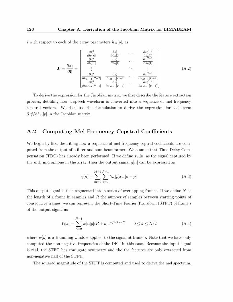
126 Chapter A. Derivation of the Jacobian Matrix for LIMABEAM
i with respect to each of the array parameters hm[p], as
Ji =∂zi∂ξ
=
∂z0i
∂h0[0]∂z1i
∂h0[0] · · · ∂zC−1i
∂h0[0]∂z0i
∂h0[1]∂z1i
∂h0[1] · · · ∂zC−1i
∂h0[1]...
.... . .
...∂z0i
∂hM−1[P−2]∂z1i
∂hM−1[P−2] · · ·∂zC−1i
∂hM−1[P−2]∂z0i
∂hM−1[P−1]∂z1i
∂hM−1[P−1] · · ·∂zC−1i
∂hM−1[P−1]
(A.2)
To derive the expression for the Jacobian matrix, we first describe the feature extraction
process, detailing how a speech waveform is converted into a sequence of mel frequency
cepstral vectors. We then use this formulation to derive the expression for each term
∂zci /∂hm[p] in the Jacobian matrix.
A.2 Computing Mel Frequency Cepstral Coefficients
We begin by first describing how a sequence of mel frequency ceptral coefficients are com-
puted from the output of a filter-and-sum beamformer. We assume that Time-Delay Com-
pensation (TDC) has already been performed. If we define xm[n] as the signal captured by
the mth microphone in the array, then the output signal y[n] can be expressed as
y[n] =M−1∑
m=0
P−1∑
p=0
hm[p]xm[n− p] (A.3)
This output signal is then segmented into a series of overlapping frames. If we define N as
the length of a frame in samples and R the number of samples between starting points of
consecutive frames, we can represent the Short-Time Fourier Transform (STFT) of frame i
of the output signal as
Yi[k] =N−1∑
n=0
w[n]y[iR+ n]e−j2πkn/N 0 ≤ k ≤ N/2 (A.4)
where w[n] is a Hamming window applied to the signal at frame i. Note that we have only
computed the non-negative frequencies of the DFT in this case. Because the input signal
is real, the STFT has conjugate symmetry and the the features are only extracted from
non-negative half of the STFT.
The squared magnitude of the STFT is computed and used to derive the mel spectrum,
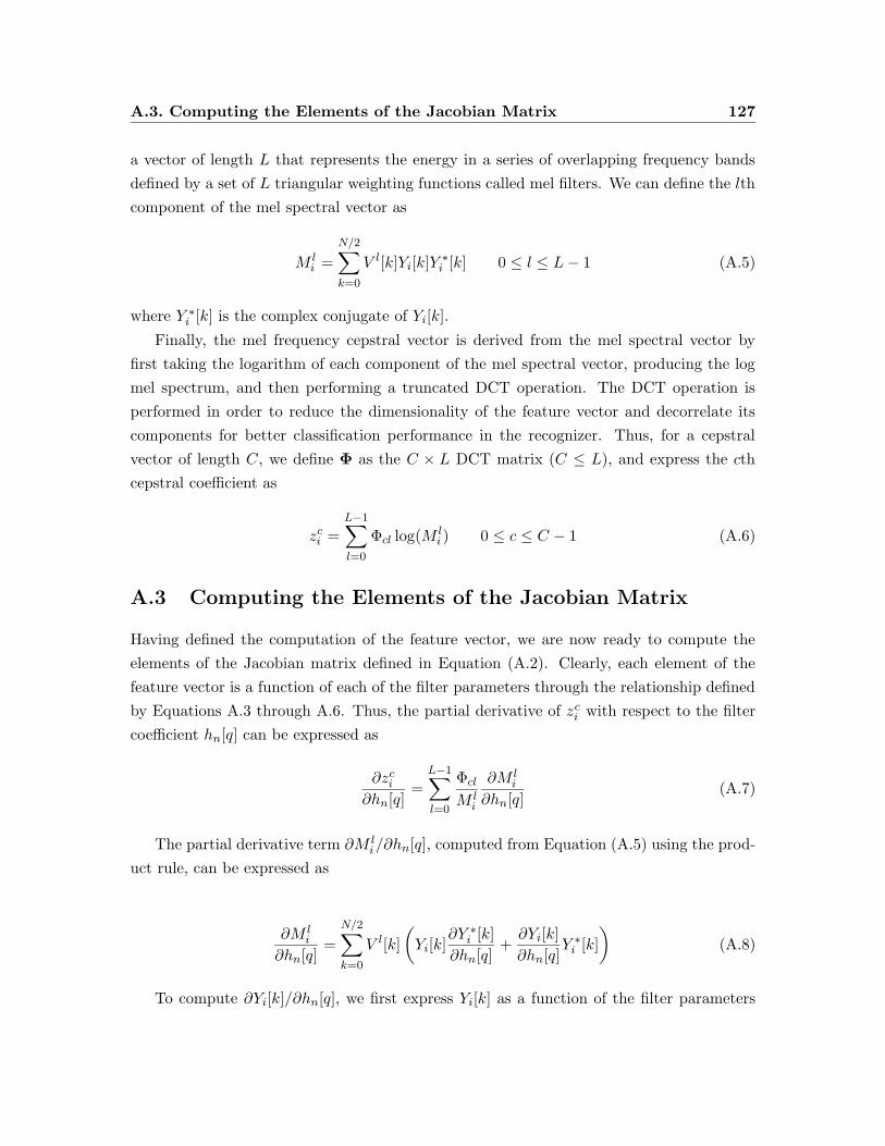
A.3. Computing the Elements of the Jacobian Matrix 127
a vector of length L that represents the energy in a series of overlapping frequency bands
defined by a set of L triangular weighting functions called mel filters. We can define the lth
component of the mel spectral vector as
M li =
N/2∑
k=0
V l[k]Yi[k]Y ∗i [k] 0 ≤ l ≤ L− 1 (A.5)
where Y ∗i [k] is the complex conjugate of Yi[k].
Finally, the mel frequency cepstral vector is derived from the mel spectral vector by
first taking the logarithm of each component of the mel spectral vector, producing the log
mel spectrum, and then performing a truncated DCT operation. The DCT operation is
performed in order to reduce the dimensionality of the feature vector and decorrelate its
components for better classification performance in the recognizer. Thus, for a cepstral
vector of length C, we define Φ as the C × L DCT matrix (C ≤ L), and express the cth
cepstral coefficient as
zci =L−1∑
l=0
Φcl log(M li ) 0 ≤ c ≤ C − 1 (A.6)
A.3 Computing the Elements of the Jacobian Matrix
Having defined the computation of the feature vector, we are now ready to compute the
elements of the Jacobian matrix defined in Equation (A.2). Clearly, each element of the
feature vector is a function of each of the filter parameters through the relationship defined
by Equations A.3 through A.6. Thus, the partial derivative of zci with respect to the filter
coefficient hn[q] can be expressed as
∂zci∂hn[q]
=L−1∑
l=0
Φcl
M li
∂M li
∂hn[q](A.7)
The partial derivative term ∂M li/∂hn[q], computed from Equation (A.5) using the prod-
uct rule, can be expressed as
∂M li
∂hn[q]=
N/2∑
k=0
V l[k]
(Yi[k]
∂Y ∗i [k]
∂hn[q]+∂Yi[k]
∂hn[q]Y ∗i [k]
)(A.8)
To compute ∂Yi[k]/∂hn[q], we first express Yi[k] as a function of the filter parameters
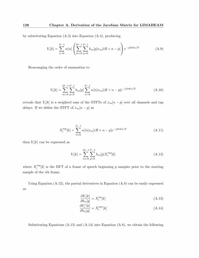
128 Chapter A. Derivation of the Jacobian Matrix for LIMABEAM
by substituting Equation (A.3) into Equation (A.4), producing
Yi[k] =N−1∑
n=0
w[n]
M−1∑
m=0
P−1∑
p=0
hm[p]xm[iR+ n− p]
e−j2πkn/N (A.9)
Rearranging the order of summation to
Yi[k] =M−1∑
m=0
P−1∑
p=0
hm[p]N−1∑
n=0
w[n]xm[iR+ n− p]e−j2πkn/N (A.10)
reveals that Yi[k] is a weighted sum of the STFTs of xm[n − p] over all channels and tap
delays. If we define the STFT of xm[n− p] as
Xmpi [k] =
N−1∑
n=0
w[n]xm[iR+ n− p]e−j2πkn/N (A.11)
then Yi[k] can be expressed as
Yi[k] =M−1∑
m=0
P−1∑
p=0
hm[p]Xmpi [k] (A.12)
where Xmpi [k] is the DFT of a frame of speech beginning p samples prior to the starting
sample of the ith frame.
Using Equation (A.12), the partial derivatives in Equation (A.8) can be easily expressed
as
∂Yi[k]
∂hn[q]= Xnq
i [k] (A.13)
∂Y ∗i [k]
∂hn[q]= Xnq∗
i [k] (A.14)
Substituting Equations (A.13) and (A.14) into Equation (A.8), we obtain the following
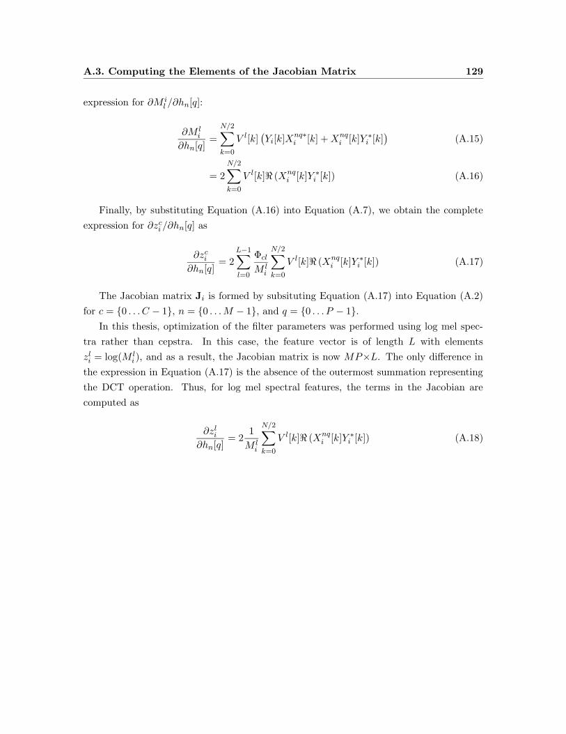
A.3. Computing the Elements of the Jacobian Matrix 129
expression for ∂M il /∂hn[q]:
∂M li
∂hn[q]=
N/2∑
k=0
V l[k](Yi[k]Xnq∗
i [k] +Xnqi [k]Y ∗i [k]
)(A.15)
= 2
N/2∑
k=0
V l[k]< (Xnqi [k]Y ∗i [k]) (A.16)
Finally, by substituting Equation (A.16) into Equation (A.7), we obtain the complete
expression for ∂zci /∂hn[q] as
∂zci∂hn[q]
= 2L−1∑
l=0
Φcl
M li
N/2∑
k=0
V l[k]< (Xnqi [k]Y ∗i [k]) (A.17)
The Jacobian matrix Ji is formed by subsituting Equation (A.17) into Equation (A.2)
for c = {0 . . . C − 1}, n = {0 . . .M − 1}, and q = {0 . . . P − 1}.In this thesis, optimization of the filter parameters was performed using log mel spec-
tra rather than cepstra. In this case, the feature vector is of length L with elements
zli = log(M li ), and as a result, the Jacobian matrix is now MP×L. The only difference in
the expression in Equation (A.17) is the absence of the outermost summation representing
the DCT operation. Thus, for log mel spectral features, the terms in the Jacobian are
computed as
∂zli∂hn[q]
= 21
M li
N/2∑
k=0
V l[k]< (Xnqi [k]Y ∗i [k]) (A.18)

Appendix B
Parameter Reduction using
ASR-based Subband Filtering
Subband processing has several advantages over the conventional fullband processing. Be-
cause the signal is divided into narrow independent subbands, the signals in each subband
can be processed independently. The subband signals have less bandwidth than the cor-
responding fullband signal and as a result, they can be downsampled prior to processing.
The combination of the independent subbands and the downsampling results in a reduction
of the number of parameters that have to be jointly estimated in a subband processing
scheme. Furthermore, a different step size can be used in each subband during adaptation,
which improves the convergence of subband adaptive filtering schemes compared to their
fullband counterparts.
In this appendix, we demonstrate the benefit of using subband filtering in speech recog-
nition applications. Specifically, we derive the reduction in parameters obtained when the
STFT is used as the analysis filterbank and the downsampling rate is governed by the frame
shift defined by the feature extraction process of the recognizer. Here, we only consider a
single channel of input. However, the results are easily generalized to the multi-microphone
case.
We define N to be length of the frame in samples and R to be the frame shift in samples,
i.e. the number of samples between starting points of consecutive frames. Given a waveform
x[n], let us define xi[n] as the ith frame of x[n]. That is,
xi[n] = x[iR+ n] (B.1)
131
132 Chapter B. Parameter Reduction using ASR-based Subband Filtering
The previous frame xi−1[n] can be similarly represented as
xi−1[n] = x[(i− 1)R+ n] (B.2)
= x[iR+ n−R] (B.3)
= xi[n−R] (B.4)
We can generalize Equation (B.4), and define the pth frame before the current frame i as
xi−p[n] = xi[n− pR] (B.5)
For notational convenience, we define the N -point discrete Fourier transform of xi[n] as
Xi = F {xi[n]} (B.6)
and the corresponding inverse discrete Fourier transform as
xi[n] = F−1 {Xi} (B.7)
where X i is a vector of length N . We refer to the kth component or frequency bin of X i
as Xi[k].
We express the subband filtering operation in the kth frequency bin as
Yi[k] =P−1∑
p=0
Hp[k]Xi−p[k] (B.8)
where Hp[k] is the pth complex filter tap of the subband filter applied to subband k. The
complete spectral output vector is formed by stacking the individual subband output signals
in Equation (B.8) for all subbands. If we define the vector operator ◦ to be the product of
the corresponding elements of two vectors, we can express this output vector, Y i, as
Y i =P−1∑
p=0
Hp ◦Xi−p (B.9)
By taking the inverse Fourier transform of Equation (B.9), we can determine the equiv-
alent time-domain representation of this subband processing operation. Thus, we have
133
yi[n] = F−1 {Y i} (B.10)
= F−1
P−1∑
p=0
Hp ◦X i−p
(B.11)
Substituting Equation (B.6) into Equation (B.11) gives
= F−1
P−1∑
p=0
Hp ◦F {xi−p[n]}
(B.12)
and using Equation (B.5) gives
= F−1
P−1∑
p=0
Hp ◦F {xi[n− pR]}
(B.13)
= F−1
P−1∑
p=0
Hp ◦F {xi[n]} ◦ e−2πpR/N (B.14)
where e−2πpR/N is a vector of the corresponding phase shift terms. Since xi[n] does not
depend on p, and the ◦ operation is commutative, we can write
= F−1
F {xi[n]} ◦
P−1∑
p=0
Hp ◦ e−2πpR/N (B.15)
Finally, if we let ⊗ represent the convolution operator, then we can write Equation (B.15)
as
= xi[n]⊗F−1
P−1∑
p=0
Hp ◦ e−2πpR/N (B.16)
= xi[n]⊗P−1∑
p=0
F−1{Hp ◦ e−2πpR/N
}(B.17)
yi[n] = xi[n]⊗
P−1∑
p=0
hp[n− pR]
(B.18)
134 Chapter B. Parameter Reduction using ASR-based Subband Filtering
The expression inside the parentheses in Equation (B.18) represents a conventional time-
domain filter equivalent to the aggegrate of all subband filters. It is the summation of P
filters, each of length N and delayed R samples, or one frame, from the previous one.
Thus, this equivalent filter spans P frames and therefore has an effective total length of
N + (P − 1) ·R samples.
In typical speech recognition applications, for speech sampled at 16 kHz, N = 400 and
R = 160, corresponding to a 25-ms frame size with a 10-ms frame shift. Using these values,
a series of 2-tap subband filters is equivalent to a fullband filter of length 400 + 160 = 560,
a series of 3-tap subband filters is equivalent to a filter of length 720, and so on. Because
each of these subband filters can be optimized independently, the number of parameters
that need to be optimized jointly is significantly reduced. This enables the parameters to
be estimated more reliably.
Appendix C
Derivation of the Gradient Vector
for S-LIMABEAM
C.1 Introduction
In this appendix, we derive the expression for the gradient vector required for S-LIMABEAM.
In this algorithm, subband filters operating on the output of a DFT filterbank are optimized
to maximize the likelihood of the resulting log mel spectra. As described in Chapter 5, the
likelihood of each component log mel spectral components is maximized independently.
Therefore, for each log mel spectral component, we require the gradient vector composed
of the partial derivatives of a particular log mel spectral coefficient with respect the each of
the filter parameters of its constituent subbands.
C.2 Defining the Gradient Vector
We define zi to be the log mel spectral feature vector of length L for frame i. Recall that
each mel spectral component is the energy in a particular frequency band defined by an
associated mel filter. Thus, the lth log mel spectral component can be expressed as
zli = log(M li ) (C.1)
= log
l+∑
k=l−
V l[k]SYi [k]
(C.2)
= log
l+∑
k=l−
V l[k]Yi[k]Y ∗i [k]
(C.3)
135
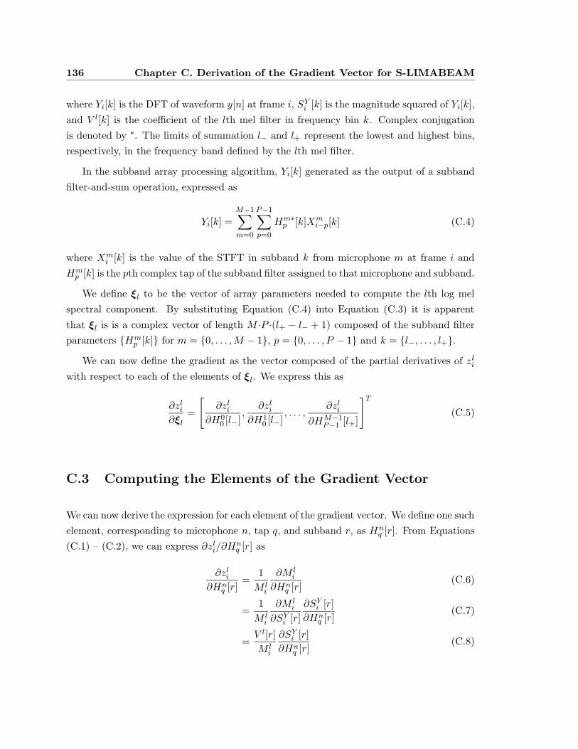
136 Chapter C. Derivation of the Gradient Vector for S-LIMABEAM
where Yi[k] is the DFT of waveform y[n] at frame i, SYi [k] is the magnitude squared of Yi[k],
and V l[k] is the coefficient of the lth mel filter in frequency bin k. Complex conjugation
is denoted by ∗. The limits of summation l− and l+ represent the lowest and highest bins,
respectively, in the frequency band defined by the lth mel filter.
In the subband array processing algorithm, Yi[k] generated as the output of a subband
filter-and-sum operation, expressed as
Yi[k] =M−1∑
m=0
P−1∑
p=0
Hm∗p [k]Xm
i−p[k] (C.4)
where Xmi [k] is the value of the STFT in subband k from microphone m at frame i and
Hmp [k] is the pth complex tap of the subband filter assigned to that microphone and subband.
We define ξl to be the vector of array parameters needed to compute the lth log mel
spectral component. By substituting Equation (C.4) into Equation (C.3) it is apparent
that ξl is is a complex vector of length M ·P ·(l+ − l− + 1) composed of the subband filter
parameters {Hmp [k]} for m = {0, . . . ,M − 1}, p = {0, . . . , P − 1} and k = {l−, . . . , l+}.
We can now define the gradient as the vector composed of the partial derivatives of z liwith respect to each of the elements of ξl. We express this as
∂zli∂ξl
=
[∂zli
∂H00 [l−]
,∂zli
∂H10 [l−]
, . . . ,∂zli
∂HM−1P−1 [l+]
]T(C.5)
C.3 Computing the Elements of the Gradient Vector
We can now derive the expression for each element of the gradient vector. We define one such
element, corresponding to microphone n, tap q, and subband r, as Hnq [r]. From Equations
(C.1) – (C.2), we can express ∂zli/∂Hnq [r] as
∂zli∂Hn
q [r]=
1
M li
∂M li
∂Hnq [r]
(C.6)
=1
M li
∂M li
∂SYi [r]
∂SYi [r]
∂Hnq [r]
(C.7)
=V l[r]
M li
∂SYi [r]
∂Hnq [r]
(C.8)
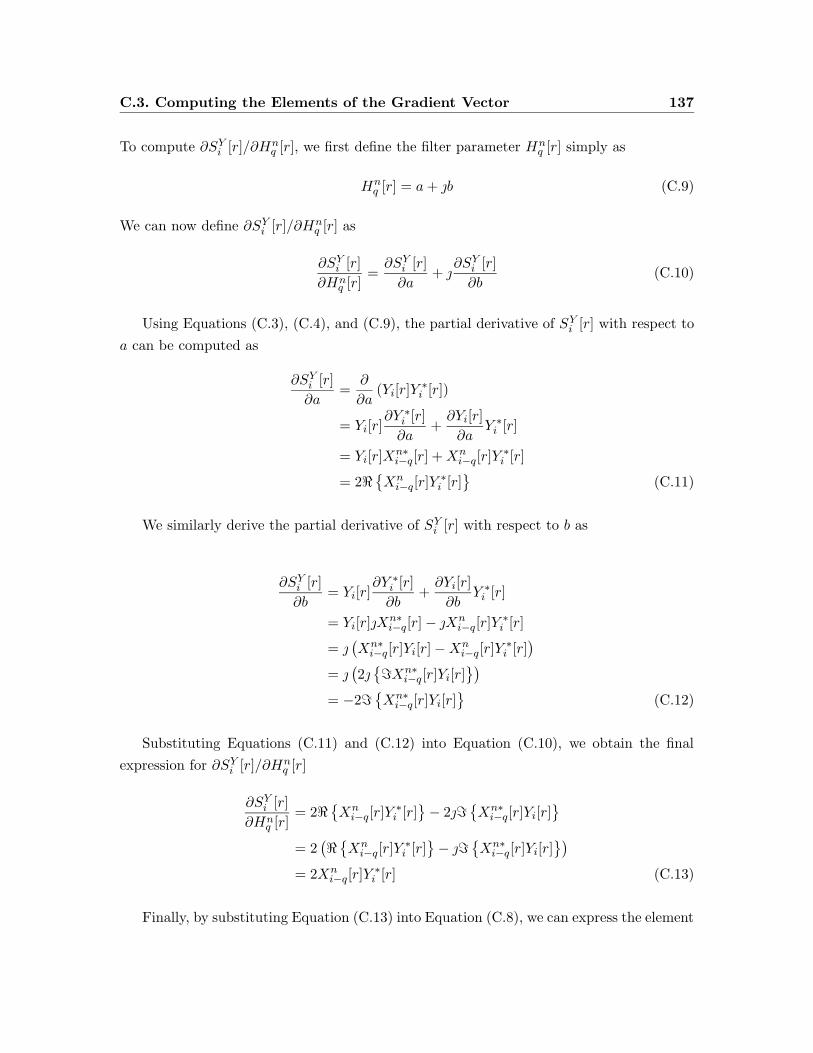
C.3. Computing the Elements of the Gradient Vector 137
To compute ∂SYi [r]/∂Hnq [r], we first define the filter parameter Hn
q [r] simply as
Hnq [r] = a+ b (C.9)
We can now define ∂SYi [r]/∂Hnq [r] as
∂SYi [r]
∂Hnq [r]
=∂SYi [r]
∂a+
∂SYi [r]
∂b(C.10)
Using Equations (C.3), (C.4), and (C.9), the partial derivative of SYi [r] with respect to
a can be computed as
∂SYi [r]
∂a=
∂
∂a(Yi[r]Y
∗i [r])
= Yi[r]∂Y ∗i [r]
∂a+∂Yi[r]
∂aY ∗i [r]
= Yi[r]Xn∗i−q[r] +Xn
i−q[r]Y∗i [r]
= 2<{Xni−q[r]Y
∗i [r]
}(C.11)
We similarly derive the partial derivative of SYi [r] with respect to b as
∂SYi [r]
∂b= Yi[r]
∂Y ∗i [r]
∂b+∂Yi[r]
∂bY ∗i [r]
= Yi[r]Xn∗i−q[r]− Xn
i−q[r]Y∗i [r]
= (Xn∗i−q[r]Yi[r]−Xn
i−q[r]Y∗i [r]
)
= (2{=Xn∗
i−q[r]Yi[r]})
= −2={Xn∗i−q[r]Yi[r]
}(C.12)
Substituting Equations (C.11) and (C.12) into Equation (C.10), we obtain the final
expression for ∂SYi [r]/∂Hnq [r]
∂SYi [r]
∂Hnq [r]
= 2<{Xni−q[r]Y
∗i [r]
}− 2=
{Xn∗i−q[r]Yi[r]
}
= 2(<{Xni−q[r]Y
∗i [r]
}− =
{Xn∗i−q[r]Yi[r]
})
= 2Xni−q[r]Y
∗i [r] (C.13)
Finally, by substituting Equation (C.13) into Equation (C.8), we can express the element
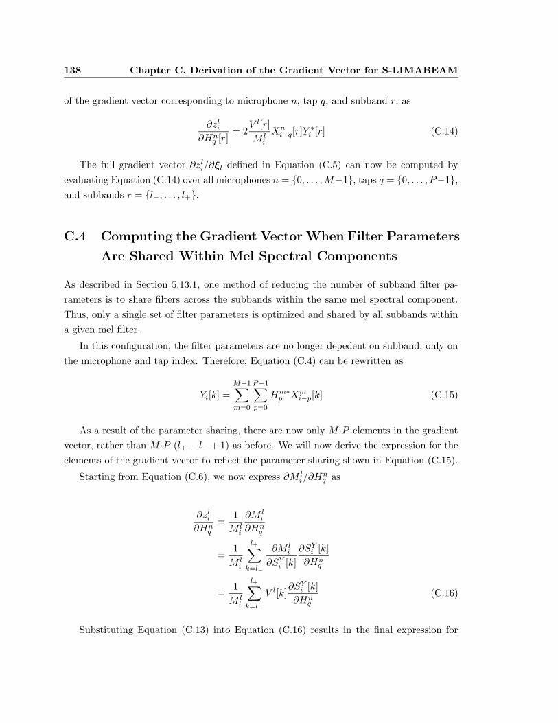
138 Chapter C. Derivation of the Gradient Vector for S-LIMABEAM
of the gradient vector corresponding to microphone n, tap q, and subband r, as
∂zli∂Hn
q [r]= 2
V l[r]
M li
Xni−q[r]Y
∗i [r] (C.14)
The full gradient vector ∂zli/∂ξl defined in Equation (C.5) can now be computed by
evaluating Equation (C.14) over all microphones n = {0, . . . ,M−1}, taps q = {0, . . . , P−1},and subbands r = {l−, . . . , l+}.
C.4 Computing the Gradient Vector When Filter Parameters
Are Shared Within Mel Spectral Components
As described in Section 5.13.1, one method of reducing the number of subband filter pa-
rameters is to share filters across the subbands within the same mel spectral component.
Thus, only a single set of filter parameters is optimized and shared by all subbands within
a given mel filter.
In this configuration, the filter parameters are no longer depedent on subband, only on
the microphone and tap index. Therefore, Equation (C.4) can be rewritten as
Yi[k] =M−1∑
m=0
P−1∑
p=0
Hm∗p Xm
i−p[k] (C.15)
As a result of the parameter sharing, there are now only M ·P elements in the gradient
vector, rather than M ·P ·(l+ − l− + 1) as before. We will now derive the expression for the
elements of the gradient vector to reflect the parameter sharing shown in Equation (C.15).
Starting from Equation (C.6), we now express ∂M li/∂H
nq as
∂zli∂Hn
q
=1
M li
∂M li
∂Hnq
=1
M li
l+∑
k=l−
∂M li
∂SYi [k]
∂SYi [k]
∂Hnq
=1
M li
l+∑
k=l−
V l[k]∂SYi [k]
∂Hnq
(C.16)
Substituting Equation (C.13) into Equation (C.16) results in the final expression for
C.5. Sharing Filter Parameters Across Mel Spectral Components 139
∂M li/∂H
nq .
∂zli∂Hn
q
= 21
M li
l+∑
k=l−
V l[k]Xni−q[k]Y ∗i [k] (C.17)
The full gradient vector is now formed by evaluating Equation (C.17) over all micro-
phones n = {0, . . . ,M − 1} and all taps q = {0, . . . , P − 1}.
C.5 Computing the Gradient Vector When Filter Parameters
Are Shared Across Mel Spectral Components
Another method of reducing the total number of parameters needed for S-LIMABEAM is
to exploit the overlap of adjacent mel filters and share subband filters across mel spectral
components, as described in Section 5.13.2. In this approach, the filter optimization is not
performed for subbands that overlap the previous mel filter. Rather, the filters resulting
from the optimization of the previous log mel spectral component are copied and used for
the current log mel component. Only the filter parameters of subbands not included in the
previous mel filter are optimized.
In this case, the gradient formulation is identical to the original unshared parameter
case. However, because the filters obtained from the previous log mel spectral component
are fixed, the gradient vector is only computed for “new” subbands that do not overlap
the previous mel filter. Therefore, the gradient vector is computed by evaluating Equation
(C.14) over all microphones n = {0, . . . ,M − 1}, taps q = {0, . . . , P − 1}, and subbands
r = {l′−, . . . , l+}, where l′− = (l − 1)+ + 1, the first subband after the highest subband of
the previous mel filter.


References
Acero, A. (1993). Acoustical and environmental robustness in automatic speech recognition.Boston, MA: Kluwer Academic Publishers.
Acero, A. (2002). personal communication.
Acero, A., Altschuler, S., & Wu, L. (2000). Speech/noise separation using two microphonesand a vq model of speech signals. Proceedings of the International Conference on SpokenLanguage Processing (pp. 532–535). Beijing, China.
Allen, J. B., & Berkley, D. A. (1979). Image method for efficiently simulating small-roomacoustics. Journal of the Acoustical Society of America, 65, 943–950.
Araki, S., Mukai, R., Makino, S., Nishikawa, T., & Saruwatari, H. (2003). The fundamentallimitation of frequency domain blind source separation for convolutive mixtures of speech.IEEE Transactions on Speech and Audio Processing, 11, 109–116.
Attias, H., Deng, L., Acero, A., & Platt, J. C. (2001). A new method for speech denoisingand robust speech recognition using probabilistic models for clean speech and for noise.Proceedings of Eurospeech (pp. 1903–1907). Aalborg, Denmark.
Bell, A. J., & Sejnowski, T. J. (1995). An information-maximization approach to blindseparation and blind deconvolution. Neural Computation, 7, 1129–1159.
Beranek, L. L. (1954). Acoustics. New York: American Institute of Physics.
Brandstein, M., & Ward, D. (Eds.). (2001). Microphone arrays - signal processing techniquesand applications. New York: Springer-Verlag.
Cox, H., Zeskind, R. M., & Owen, M. M. (1987). Robust adaptive beamforming. IEEETransactions on Acoustics, Speech, and Signal Processing, ASSP-35, 1365–1376.
Cutler, R., Rui, Y., Gupta, A., Cadiz, J. J., Tashev, I., wei He, L., Colburn, A., Zhang, Z.,Liu, Z., & Silverberg, S. (2002). Distributed meetings: A meeting capture and broadcast-ing system. Proceedings of ACM Multimedia. Juan Les Pins, France.
Davis, S., & Mermelstein, P. (1980). Comparison of parametric representation for monosylla-blic word recognition in continuously spoken sentences. IEEE Transactions on Acoustics,Speech, and Signal Processing, 28, 357–366.
141
142 References
de Haan, J. M., Grbic, N., Claesson, I., & Nordholm, S. (2002). Design and evaluation ofnonuniform DFT filter banks in subband microphone arrays. Proceedings of the IEEEInternational Conference on Acoustics, Speech, and Signal Processing (pp. 1173–1176).Orlando, FL.
Deng, L., Wang, K., Acero, A., Hon, H., Droppo, J., Boulis, C., Wang, Y., Jacoby, D.,Mahajan, M., Chelba, C., & Huang, X. D. (2002). Distributed speech processing inmiPad’s multimodal user interface. IEEE Transactions on Speech and Audio Processing,10, 605–619.
Flanagan, J. L., Berkely, D. A., Elko, G. W., West, J. E., & Sondhi, M. M. (1991). Autodi-rective microphone arrays. Acustica, 73, 58–71.
Flanagan, J. L., Johnston, J. D., Zahn, R., & Elko, G. W. (1985). Computer-steeredmicrophone arrays for sound transduction in large rooms. Journal of the Acoustical Societyof America, 78, 1508–1518.
Flanagan, J. L., Surendran, A. C., & Jan, E. E. (1993). Spatially selective sound capturefor speech and audio processing. Speech Communication, 13, 207–222.
Frost, O. L. (1972). An algorithm for linearly constrained adaptive array processing. Pro-ceedings of the IEEE, 60, 926–935.
Gillespie, B., & Atlas, L. E. (2002). Acoustic diversity for improved speech recognition in re-verberant environments. Proceedings of the IEEE International Conference on Acoustics,Speech, and Signal Processing (pp. 557–560). Orlando, FL.
Gillespie, B., Malvar, H., & Florncio, D. (2001). Speech dereverberation via maximumkurtosis subband adaptive filtering. Proceedings of the IEEE International Conference onAcoustics, Speech, and Signal Processing (pp. 3701 –3704). Salt Lake City, UT.
Gillick, L., & Cox, S. J. (1989). Some statistical issues in the comparison of speech recogni-tion algorithms. Proceedings of the IEEE International Conference on Acoustics, Speech,and Signal Processing (pp. 532–535). Glasgow, UK.
Gilloire, A., & Vetterli, M. (1992). Adaptive filtering in subbands with critical sampling:analysis, experiments and application to acoustic echo cancellation. IEEE Transactionson Signal Processing, 40, 1862–1875.
Giuliani, D., Matassoni, M., Omologo, M., & Svaizer, P. (1998). Experiments of HMMadaptation for hands-free connected digit recognition. Proceedings of the IEEE Interna-tional Conference on Acoustics, Speech, and Signal Processing (pp. 473–476). Seattle,WA.
Griffiths, L. J., & Jim, C. W. (1982). An alternative approach to linearly constrainedadaptive beamforming. IEEE Transactions on Antennas and Propagation, AP-30, 27–34.
Haykin, S. (2002). Adaptive filter theory. New Jersey: Prentice Hall.
References 143
Hazen, T. J., Seneff, S., & Polifroni, J. (2002). Recognition confidence scoring and its usein speech understanding systems. Computer Speech & Language, 16, 49–67.
Hoshuyama, O., Sugiyama, A., & Hirano, A. (1999). A robust adaptive beamformer formicrophone arrays with a blocking matrix using constrained adaptive filters. IEEE Trans-actions on Signal Processing, 47, 2677 –2684.
Hughes, T. B., Kim, H. S., DiBiase, J. H., & Silverman, H. F. (1999). Performance ofan HMM speech recognizer using a real-time tracking microphone array as input. IEEETransactions on Speech and Audio Processing, 7, 346–349.
Hwang, M.-Y. (1993). Subphonetic acoustic modeling for speaker-independent conitnuousspeech recognition. Doctoral dissertation, Carnegie Mellon University, Pittsburgh, PA.
Hwang, M.-Y., & Huang, X. (1993). Shared-distribution hidden Markov models for speechrecognition. IEEE Transactions on Speech and Audio Processing, 1, 414–420.
Janin, A., Baron, D., Edwards, J., Ellis, D., Gelbart, D., Morgan, N., Peskin, B., Pfau, T.,Shriberg, E., Stolcke, A., & Wooters, C. (2003). The ICSI meeting corpus. Proceedingsof the IEEE International Conference on Acoustics, Speech, and Signal Processing (pp.364–367). Hong Kong.
Jelinek, F. (1997). Statistical methods for speech recognition. Cambridge, MA: MIT Press.
Johnson, D. H., & Dudgeon, D. E. (1993). Array signal processing. New Jersey: PrenticeHall.
Kajala, M., & Hamalainen, M. (1999). Broadband beamforming optimization for speech en-hancement in noisy environments. Proceedings of the IEEE Workshop in the Applicationsof Signal Processing to Audio and Acoustics (pp. 19–22). New Paltz, NY.
Knapp, C. H., & Carter, C. (1976). The generalized correlation method for estimation oftime delay. IEEE Transactions on Acoustics, Speech, and Signal Processing, ASSP-24,320–327.
Kurita, S., Sauwatari, H., Kajita, S., Takeda, K., & Itakura, F. (2000). Evaluation of blindsignal separation method using directivity pattern under reverberant conditions. Proceed-ings of the IEEE International Conference on Acoustics, Speech, and Signal Processing(pp. 3140–3143). Istanbul, Turkey.
Leggetter, C. J., & Woodland, P. C. (1994). Speaker adaptation of HMMs using linear regres-sion (Technical Report CUED/F-INFENG/ TR. 181). Cambridge University, Cambridge,UK.
Liu, F.-H., Acero, A., & Stern, R. M. (1992). Efficient joint compensation of speech forthe effects of additive noise and linear filtering. Proceedings of the IEEE InternationalConference on Acoustics, Speech, and Signal Processing (pp. 257–260). San Francisco,CA.
144 References
Liu, Q.-G., Champagne, B., & Kabal, P. (1996). A microphone array processing techniquefor speech enhancement in a reverberant space. Speech Communication, 18, 317–334.
Liu, W., Weiss, S., & Hanzo, L. (2001). Subband adaptive generalized sidelobe cancellerfor broadband beamforming. Proceedings of the IEEE Workshop on Statistical SignalProcessing (pp. 591–594). Singapore.
Malvar, H. A. (2002). personal communication.
Marro, C., Mahieux, Y., & Simmer, K. U. (1998). Analysis of noise reduction and derever-beration techniques based on microphone arrays with postfiltering. IEEE Transactionson Speech and Audio Processing, 6, 240–259.
Miyoshi, M., & Kaneda, Y. (1988). Inverse filtering of room acoustics. IEEE Transactionson Speech and Audio Processing, 36, 145–152.
Moreno, P. (1996). Speech recognition in noisy environments. Doctoral dissertation,Carnegie Mellon University, Pittsburgh, PA.
Moreno, P., Raj, B., & Stern, R. M. (1995). A unified approach for robust speech recogni-tion. Proceedings of Eurospeech (pp. 481–485). Madrid, Spain.
Morgan, N., Baron, D., Bhagatl, S., Carvey, H., Dhillon, R., Edwards, J., Gelbart, D.,Janin, A., Krupskil, A., Peskin, B., Pfau, T., Shriberg, E., Stolcke, A., & Wooters, C.(2003). Meetings about meetings: research at ICSI on speech in multiparty conversations.Proceedings of the IEEE International Conference on Acoustics, Speech, and Signal Pro-cessing (pp. 740–743). Hong Kong.
Nakamura, S., Hiyane, K., Asano, F., Nishiura, T., & Yamada, T. (2000). Acoustical soundscene database in real environments for sound scene understanding and hands-free speechrecognition. International Conference on Language Resources and Evaluation. Athens,Greece.
Nawab, S. H., & Quatieri, T. F. (1988). Advanced topics in signal processing, chapterShort-Time Fourier Transform, 289–337. New Jersey: Prentice Hall.
Neely, S., & Allen, J. (1979). Invertibility of a room impulse response. Journal of theAcoustical Society of America, 66, 165–169.
Neo, W. H., & Farhang-Boroujeny, B. (2001). Robust microphone arrays using subbandadaptive filters. Proceedings of the IEEE International Conference on Acoustics, Speech,and Signal Processing (pp. 3721–3724). Salt Lake City, UT.
Nocedal, J., & Wright, S. (1999). Numerical optimization. New York: Springer.
Nordholm, S., Claesson, I., & Dahl, M. (1999). Adaptive microphone array employingcalibration signals. IEEE Transactions on Speech and Audio Processing, 7, 241–252.
References 145
Omologo, M., Matassoni, M., Svaizer, P., & Giuliani, D. (1997). Experiments of hands-freeconnected digit recognition using a microphone array. Proceedings of the IEEE Workshopon Automatic Speech Recognition and Understanding (pp. 490–497). Santa Barbara, CA.
Pallett, D. S., Fiscus, J. G., Fisher, W. M., Garofolo, J. S., Martin, A. F., & Przybocki,M. A. (1996). 1995 HUB-3 NIST multiple microphone corpus benchmark tests. Proceed-ings of the ARPA Speech Recognition Workshop (pp. 27–46). Harriman, NY.
Paul, D. B., & Baker, J. M. (1992). The design of the Wall Street Journal-based CSRcorpus. Proceedings of the ARPA Speech and Natural Language Workshop (pp. 357–362).Harriman, NY.
Placeway, P., Chen, S., Eskenazi, M., Jain, U., Parikh, V., Raj, B., Ravishankar, M.,Rosenfeld, R., Seymore, K., Siegler, M., Stern, R., & Thayer, E. (1997). The 1996 hub-4sphinx-3 system. Proceedings of the DARPA Speech Recognition workshop.
Pradhan, S. S., & Reddy, V. U. (1999). A new approach to subband adaptive filtering.IEEE Transactions on Signal Processing, 47, 655–664.
Putnam, W., Rocchesso, D., & Smith, J. (1995). A numerical investigation of the invertibil-ity of room transfer functions. Proceedings of the IEEE ASSP Workshop on Applicationsof Signal Processing to Audio and Acoustics (pp. 249–252). Mohonk, NY.
Rabiner, L., & Juang, B.-H. (1993). Fundamentals of speech recognition. New Jersey:Prentice Hall.
Rabinkin, D., Renomeron, R., & Flanagan, J. (1997). Microphone array sensor placementoptimization in reverberant environments. Journal of the Acoustical Society of America,102, 3207.
Rudnicky, A., Thayer, E., Constantinides, P., Tchou, C., Shern, R., Lenzo, K., Xu, W., &Oh, A. (1999). Creating natural dialogs in the Carnegie Mellon Communicator system.Proceedings of Eurospeech (pp. 1531–1534). Budapest, Hungary.
Sanders, G. A., Le, A. N., & Garofolo, J. S. (2002). Effects of word error rate in the DARPACommunicator data during 2000 and 2001. Proceedings of the International Conferenceon Spoken Language Processing (pp. 277–280). Denver, Colorado.
Seltzer, M., & Raj, B. (2001). Calibration of microphone arrays for improved speech recog-nition. Proceedings of Eurospeech (pp. 1005–1008). Aalborg, Denmark.
Seltzer, M. L., Raj, B., & Stern, R. M. (2002). Speech recognizer-based microphone arrayprocessing for robust hands-free speech recognition. Proceedings of the IEEE InternationalConference on Acoustics, Speech, and Signal Processing (pp. 897–900). Orlando, FL.
Seltzer, M. L., & Stern, R. M. (2003). Subband parameter optimization of microphone arraysfor speech recognition in reverberant environments. Proceedings of the IEEE InternationalConference on Acoustics, Speech, and Signal Processing (pp. 408–411). Hong Kong.
146 References
Silverman, H. F., Patterson, W. R., & Flanagan, J. L. (1996). The huge microphone array(HMA) (Technical Report). Brown University, Providence, RI.
Sullivan, T. M. (1996). Multi-microphone correlation-based processing for robust speechrecognition. Doctoral dissertation, Carnegie Mellon University, Pittsburgh, PA.
Sullivan, T. M., & Stern, R. M. (1993). Multi-microphone correlation-based processing forrobust speech recognition. Proceedings of the IEEE International Conference on Acous-tics, Speech, and Signal Processing (pp. 27–30). Minneapolis, MN.
Suzuki, Y., Asano, F., Kim, H.-Y., & Sone, T. (1995). An optimum computer-generatedpulse signal suitable for the measurement of very long impulse responses. Journal of theAcoustical Society of America, 97, 1119–1123.
Van Compernolle, D. (1990). Switching adaptive filters for enhancing noisy and reverberantspeech from microphone array recordings. Proceedings of the IEEE International Confer-ence on Acoustics, Speech, and Signal Processing (pp. 833–836). Albequerque, NM.
Viterbi, A. J. (1967). Error bounds for convolutional codes and an asymptotically optimumdecoding algorithm. IEEE Transactions on Information Theory, 13, 260–269.
Waibel, A., Bett, M., Metze, F., Ries, K., Schaaf, T., Schultz, T., Soltau, H., Yu, H., &Zechner, K. (2001). Advances in automatic meeting record creation and access. Proceed-ings of the IEEE International Conference on Acoustics, Speech, and Signal Processing(pp. 597–600). Salt Lake City, UT.
Walker, M. A., Rudnicky, A., Prasad, R., Aberdeen, J., Bratt, E. O., Garofolo, J., Hastie,H., Le, A., Pellom, B., Potamianos, A., Passonneau, R., Roukos, S., Sanders, G., Seneff,S., & Stallard, D. (2002). DARPA Communicator: cross-system results for the 2001evaluation. Proceedings of the International Conference on Spoken Language Processing(pp. 269–272). Denver, Colorado.
Woodland, P. C., Gales, M. J. F., & Pye, D. (1996). Improving environmental robustness inlarge vocabulary speech recognition. Proceedings of the IEEE International Conferenceon Acoustics, Speech, and Signal Processing (pp. 65–69). Atlanta, GA.
Zelinkski, R. (1988). A microphone array with adaptive post-filtering for noise reductionin reverberant rooms. Proceedings of the IEEE International Conference on Acoustics,Speech, and Signal Processing (pp. 2578–2581). New York, NY.