Micromechanics and Stress Analysis of a Composite Cylinder

Created in COMSOL Multiphysics 5.6

M i c r ome chan i c s and S t r e s s Ana l y s i s o f aCompo s i t e C y l i n d e r

This model is licensed under the COMSOL Software License Agreement 5.6.All trademarks are the property of their respective owners. See www.comsol.com/trademarks.

http://www.comsol.com/sla

http://www.comsol.com/trademarks/

Introduction

The use of fiber composites in the manufacturing industry is increasing. Compared to traditional metallic engineering materials, fiber composites are lighter and more corrosion resistant, and properties like strength, stiffness and toughness can often be tailored to a specific application. A fiber composite consists of load carrying fibers embedded in a polymer resin. The composite material is typically a laminate of individual layers, where the fibers in each layer are uni-directional. In this model, we perform a stress analysis of a laminated composite cylinder.

Modeling individual fibers in every layer in the laminate is unfeasible. A simplified micromechanics model of a single carbon fiber in epoxy is instead used to estimate the elastic properties of a single layer. These properties are then used in the homogenized model of the laminated composite cylinder. Two approaches are used to model the laminate, namely the Layerwise (LW) theory, and the Equivalent Single Layer (ESL) theory.

Model Definition

This model performs different types of analyses of a laminated composite cylinder. The model is divided into three parts:

• Micromechanics analysis

• Stress analysis using the Layerwise theory

• Stress analysis using the Equivalent Single Layer theory

Eigenfrequencies and mode shapes are computed and compared using both theories.

M I C R O M E C H A N I C S A N A L Y S I S

A micromechanics analysis of a single layer is performed in order to obtain its homogenized material properties. The composite layer is assumed to be made of carbon fibers unidirectionally embedded in epoxy resin. A representative unit cell having a cylindrical fiber located at the middle of resin is shown in Figure 1. The fiber radius is computed assuming a fiber volume fraction of 0.6.

2 | M I C R O M E C H A N I C S A N D S T R E S S A N A L Y S I S O F A C O M P O S I T E C Y L I N D E R

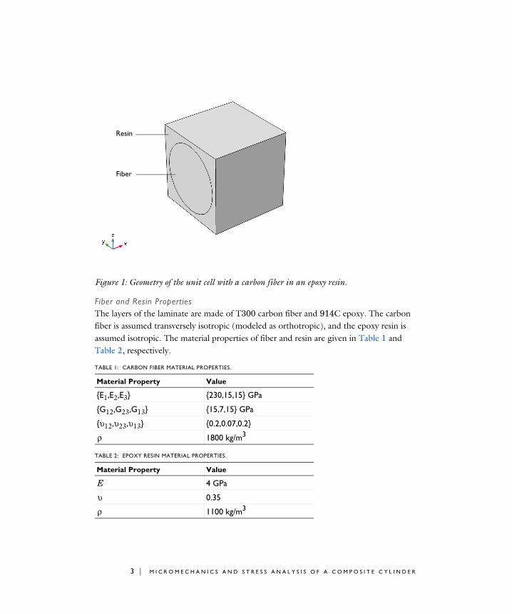
Figure 1: Geometry of the unit cell with a carbon fiber in an epoxy resin.

Fiber and Resin PropertiesThe layers of the laminate are made of T300 carbon fiber and 914C epoxy. The carbon fiber is assumed transversely isotropic (modeled as orthotropic), and the epoxy resin is assumed isotropic. The material properties of fiber and resin are given in Table 1 and Table 2, respectively.

TABLE 1: CARBON FIBER MATERIAL PROPERTIES.

Material Property Value

{E1,E2,E3} {230,15,15} GPa

{G12,G23,G13} {15,7,15} GPa

{υ12,υ23,υ13} {0.2,0.07,0.2}

ρ 1800 kg/m3

TABLE 2: EPOXY RESIN MATERIAL PROPERTIES.

Material Property Value

E 4 GPa

υ 0.35

ρ 1100 kg/m3

Fiber

Resin


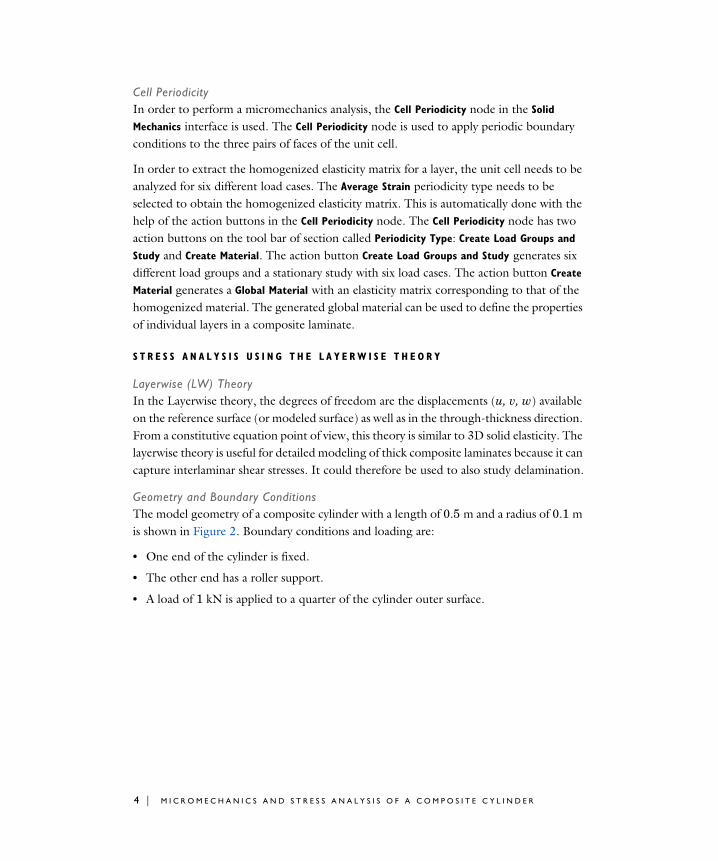
Cell PeriodicityIn order to perform a micromechanics analysis, the Cell Periodicity node in the Solid

Mechanics interface is used. The Cell Periodicity node is used to apply periodic boundary conditions to the three pairs of faces of the unit cell.

In order to extract the homogenized elasticity matrix for a layer, the unit cell needs to be analyzed for six different load cases. The Average Strain periodicity type needs to be selected to obtain the homogenized elasticity matrix. This is automatically done with the help of the action buttons in the Cell Periodicity node. The Cell Periodicity node has two action buttons on the tool bar of section called Periodicity Type: Create Load Groups and

Study and Create Material. The action button Create Load Groups and Study generates six different load groups and a stationary study with six load cases. The action button Create

Material generates a Global Material with an elasticity matrix corresponding to that of the homogenized material. The generated global material can be used to define the properties of individual layers in a composite laminate.

S T R E S S A N A L Y S I S U S I N G T H E L A Y E R W I S E T H E O R Y

Layerwise (LW) Theory In the Layerwise theory, the degrees of freedom are the displacements (u, v, w) available on the reference surface (or modeled surface) as well as in the through-thickness direction. From a constitutive equation point of view, this theory is similar to 3D solid elasticity. The layerwise theory is useful for detailed modeling of thick composite laminates because it can capture interlaminar shear stresses. It could therefore be used to also study delamination.

Geometry and Boundary ConditionsThe model geometry of a composite cylinder with a length of 0.5 m and a radius of 0.1 m is shown in Figure 2. Boundary conditions and loading are:

• One end of the cylinder is fixed.

• The other end has a roller support.

• A load of 1 kN is applied to a quarter of the cylinder outer surface.


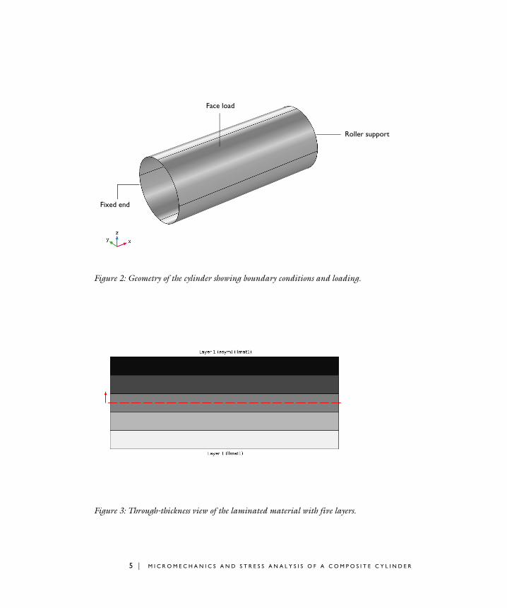
Figure 2: Geometry of the cylinder showing boundary conditions and loading.

Figure 3: Through-thickness view of the laminated material with five layers.

Fixed end

Roller support

Face load


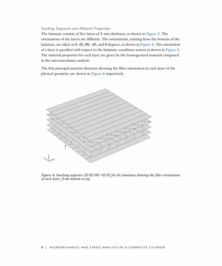
Stacking Sequence and Material PropertiesThe laminate consists of five layers of 1 mm thickness, as shown in Figure 3. The orientations of the layers are different. The orientations, starting from the bottom of the laminate, are taken as 0, 45, 90, -45, and 0 degrees, as shown in Figure 4. The orientation of a layer is specified with respect to the laminate coordinate system as shown in Figure 5. The material properties for each layer are given by the homogenized material computed in the micromechanics analysis.

The first principal material direction showing the fiber orientation in each layer of the physical geometry are shown in Figure 6 respectively.

Figure 4: Stacking sequence [0/45/90/-45/0] for the laminate showing the fiber orientation of each layer, from bottom to top.


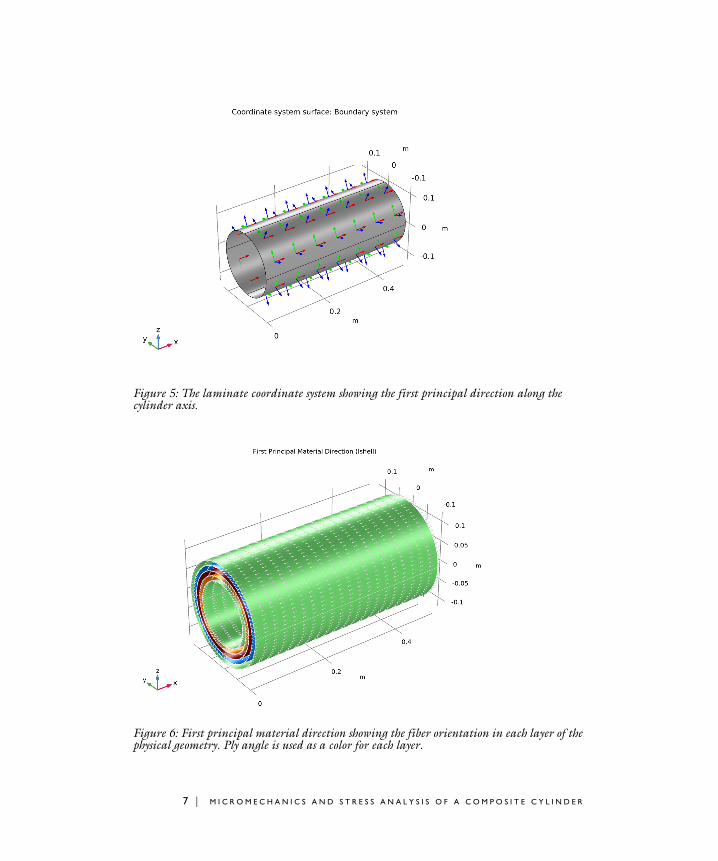
Figure 5: The laminate coordinate system showing the first principal direction along the cylinder axis.

Figure 6: First principal material direction showing the fiber orientation in each layer of the physical geometry. Ply angle is used as a color for each layer.


S T R E S S A N A L Y S I S U S I N G T H E E S L T H E O R Y

Equivalent Single Layer (ESL) TheoryIn the equivalent single layer (ESL) theory, the degrees of freedom are the displacements and rotations on the midplane of the laminate. From a constitutive equation point of view, this theory is similar to 3D shell elasticity. Through-thickness homogenized material properties of the laminate are used. It is therefore computationally less expensive than the layerwise theory. It can be used for the modeling of thin to moderately thick laminates with good accuracy. An aim of this analysis is to compare the results to the results obtained from the layerwise theory.

The model setup, including geometry, boundary conditions, material properties, and so on, is the same as described in the previous section.

Results and Discussion

In the micromechanics analysis, six load cases are used to evaluate the elasticity matrix. The distribution of effective (von Mises) stress for four of the load cases is shown in Figure 7.


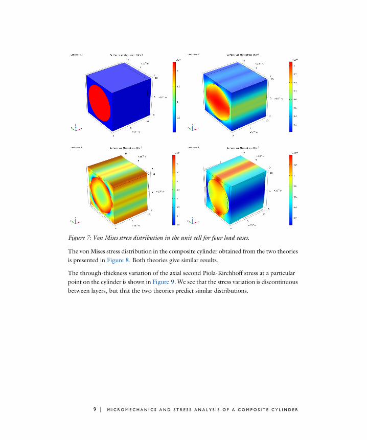
Figure 7: Von Mises stress distribution in the unit cell for four load cases.

The von Mises stress distribution in the composite cylinder obtained from the two theories is presented in Figure 8. Both theories give similar results.

The through-thickness variation of the axial second Piola-Kirchhoff stress at a particular point on the cylinder is shown in Figure 9. We see that the stress variation is discontinuous between layers, but that the two theories predict similar distributions.


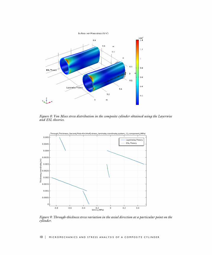
Figure 8: Von Mises stress distribution in the composite cylinder obtained using the Layerwise and ESL theories.

Figure 9: Through-thickness stress variation in the axial direction at a particular point on the cylinder.


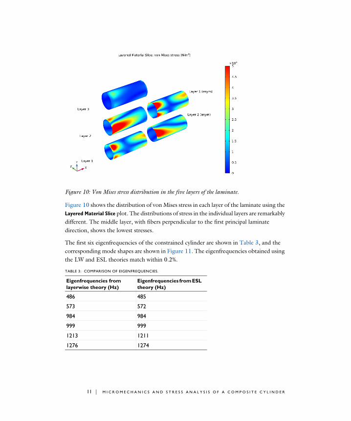
Figure 10: Von Mises stress distribution in the five layers of the laminate.

Figure 10 shows the distribution of von Mises stress in each layer of the laminate using the Layered Material Slice plot. The distributions of stress in the individual layers are remarkably different. The middle layer, with fibers perpendicular to the first principal laminate direction, shows the lowest stresses.

The first six eigenfrequencies of the constrained cylinder are shown in Table 3, and the corresponding mode shapes are shown in Figure 11. The eigenfrequencies obtained using the LW and ESL theories match within 0.2%.

TABLE 3: COMPARISON OF EIGENFREQUENCIES.

Eigenfrequencies from layerwise theory (Hz)

Eigenfrequencies from ESL theory (Hz)

486 485

573 572

984 984

999 999

1213 1211

1276 1274


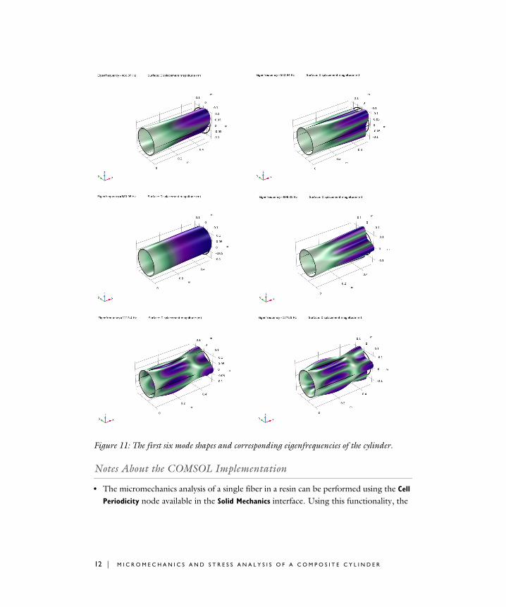
Figure 11: The first six mode shapes and corresponding eigenfrequencies of the cylinder.

Notes About the COMSOL Implementation

• The micromechanics analysis of a single fiber in a resin can be performed using the Cell

Periodicity node available in the Solid Mechanics interface. Using this functionality, the


elasticity matrix of the homogenized material can be computed for the given fiber and resin properties, and the fiber volume fraction.

• The Cell Periodicity node has two action buttons on the tool bar of section called Periodicity Type: Create Load Groups and Study and Create Material. The action button Create Load Groups and Study generates load groups and a stationary study with loadcases. The action button Create Material generate a Global Material with homogenized material properties. The action buttons are active depending on the choices in the Periodicity Type and Calculate Average Properties lists.

• Modeling a composite laminated shell requires a surface geometry (2D), in general called a base surface, and a Layered Material node which adds an extra dimension (1D) to the base surface geometry in the surface normal direction. Using the Layered Material functionality, you can model several layers of different thickness, material properties, and fiber orientations. You can optionally specify the interface materials between the layers and the control mesh elements in each layer.

• The Layered Material Link and Layered Material Stack have an option to transform the given Layered Material into a symmetric or antisymmetric laminate. A repeated laminate can also be constructed using a transform option.

• You can either use the Layerwise (LW) theory based Layered Shell interface or the Equivalent Single Layer (ESL) theory based Layered Linear Elastic Material node in Shell interface.

• To analyze the results in a composite shell, you can either create a slice plot using the Layered Material Slice plot for in-plane variation of a quantity, or you can create a Through

Thickness plot for out-of-plane variation of a quantity. To visualize the results as a 3D solid object, you can use the Layered Material dataset which creates a virtual 3D solid object combining the surface geometry (2D) and the extra dimension (1D).

Application Library path: Composite_Materials_Module/Tutorials/composite_cylinder_micromechanics_and_stress_analysis

Modeling Instructions (Micromechanics)

From the File menu, choose New.

N E W

In the New window, click Model Wizard.


M O D E L W I Z A R D

1 In the Model Wizard window, click 3D.

2 In the Select Physics tree, select Structural Mechanics>Solid Mechanics (solid).

3 Click Add.

4 Click Done.

G L O B A L D E F I N I T I O N S

Parameters 11 In the Model Builder window, under Global Definitions click Parameters 1.

2 In the Settings window for Parameters, locate the Parameters section.

3 Click Load from File.

4 Browse to the model’s Application Libraries folder and double-click the file composite_cylinder_micromechanics_and_stress_analysis_parameters.txt.

G E O M E T R Y 1

Block 1 (blk1)1 In the Geometry toolbar, click Block.

2 In the Settings window for Block, locate the Size and Shape section.

3 In the Width text field, type l.

4 In the Depth text field, type l.

5 In the Height text field, type l.

6 Click Build Selected.

Cylinder 1 (cyl1)1 In the Geometry toolbar, click Cylinder.

2 In the Settings window for Cylinder, locate the Size and Shape section.

3 In the Radius text field, type r_f.

4 In the Height text field, type l.

5 Locate the Position section. In the y text field, type l/2.

6 In the z text field, type l/2.

7 Locate the Axis section. From the Axis type list, choose x-axis.



Form Union (fin)1 In the Model Builder window, click Form Union (fin).

2 In the Settings window for Form Union/Assembly, click Build Selected.

S O L I D M E C H A N I C S ( S O L I D )

Cell Periodicity 11 In the Model Builder window, under Component 1 (comp1) right-click

Solid Mechanics (solid) and choose the domain setting More>Cell Periodicity.

2 In the Settings window for Cell Periodicity, locate the Domain Selection section.

3 From the Selection list, choose All domains.

4 Locate the Periodicity Type section. From the list, choose Average strain.

5 From the Calculate average properties list, choose Elasticity matrix, Standard (XX, YY, ZZ,

XY, YZ, XZ).

Boundary Pair 11 In the Physics toolbar, click Attributes and choose Boundary Pair.

2 In the Settings window for Boundary Pair, locate the Boundary Selection section.

3 Click Clear Selection.

4 Select Boundaries 1, 5, 11, and 12 only.

Boundary Pair 21 Right-click Boundary Pair 1 and choose Duplicate.



4 Select Boundaries 2 and 10 only.

Boundary Pair 31 Right-click Boundary Pair 2 and choose Duplicate.




In the upper-right corner of the Periodicity type section, you can find two buttons Create Load Groups and Study and Create Material. When the Average strain option is selected for computation of elasticity matrix, you can automatically generate load groups, a study, and a material by clicking on these buttons.


Cell Periodicity 11 In the Model Builder window, click Cell Periodicity 1.

2 In the Settings window for Cell Periodicity, click Study and Material Generation in the upper-right corner of the Periodicity Type section. From the menu, choose Create Load Groups and Study to generate load groups and a study nodes.

3 Click Study and Material Generation in the upper-right corner of the Periodicity Type section. From the menu, choose Create Material to generate a global material node with computed elastic properties.

M A T E R I A L S

Material 1: Epoxy Resin1 In the Model Builder window, under Component 1 (comp1) right-click Materials and

choose Blank Material.

Before adding the fiber material data, set the solid model to orthotropic in the Linear

Elastic Material node since the fiber material is assumed to have orthotropic properties. The isotropic resin material data will be automatically converted into an orthotropic format.

2 In the Settings window for Material, type Material 1: Epoxy Resin in the Label text field.

3 Select Domain 1 only.

4 Locate the Material Contents section. In the table, enter the following settings:

S O L I D M E C H A N I C S ( S O L I D )

Linear Elastic Material 11 In the Model Builder window, under Component 1 (comp1)>Solid Mechanics (solid) click

Linear Elastic Material 1.

2 In the Settings window for Linear Elastic Material, locate the Linear Elastic Material section.

3 From the Solid model list, choose Orthotropic.

Property Variable Value Unit Property group

Young’s modulus E E_r Pa Basic

Poisson’s ratio nu nu_r 1 Basic

Density rho rho_r kg/m³ Basic


M A T E R I A L S

Material 2: Carbon Fiber1 In the Model Builder window, under Component 1 (comp1) right-click Materials and

choose Blank Material.

2 In the Settings window for Material, type Material 2: Carbon Fiber in the Label text field.

3 Locate the Geometric Entity Selection section. Click Paste Selection.

4 In the Paste Selection dialog box, type 2 in the Selection text field.

5 Click OK.

6 In the Settings window for Material, locate the Material Contents section.

7 In the table, enter the following settings:

M E S H 1

Free Triangular 11 In the Mesh toolbar, click Boundary and choose Free Triangular.


3 In the Settings window for Free Triangular, click Build Selected.

Swept 11 In the Mesh toolbar, click Swept.

2 In the Settings window for Swept, click Build Selected.

C E L L P E R I O D I C I T Y S T U D Y

In the Home toolbar, click Compute.


Young’s modulus

{Evector1, Evector2, Evector3}

{E1_f, E2_f, E2_f}

Pa Orthotropic

Poisson’s ratio

{nuvector1, nuvector2, nuvector3}

{nu12_f, nu23_f, nu12_f}

1 Orthotropic

Shear modulus

{Gvector1, Gvector2, Gvector3}

{G12_f, G23_f, G12_f}

N/m² Orthotropic

Density rho rho_f kg/m³ Basic


R E S U L T S

Stress, Unit CellUse the following instructions to plot the von Mises stress in the unit cell as shown in Figure 7.

1 In the Settings window for 3D Plot Group, type Stress, Unit Cell in the Label text field.

2 In the Stress, Unit Cell toolbar, click Plot.

Modeling Instructions (Stress Analysis using the Layerwise (LW) Theory)

This section describes how to model a laminated composite cylinder using the layerwise theory based Layered Shell interface.

A D D C O M P O N E N T

In the Model Builder window, right-click the root node and choose Add Component>3D.

G E O M E T R Y 2

Cylinder 1 (cyl1)1 In the Geometry toolbar, click Cylinder.

2 In the Settings window for Cylinder, locate the Object Type section.

3 From the Type list, choose Surface.

4 Locate the Size and Shape section. In the Radius text field, type rc.

5 In the Height text field, type hc.

6 Locate the Axis section. From the Axis type list, choose x-axis.


D E F I N I T I O N S ( C O M P 2 )

Boundary System 2 (sys2)1 In the Model Builder window, expand the Component 2 (comp2)>Definitions node, then

click Boundary System 2 (sys2).

2 In the Settings window for Boundary System, locate the Settings section.

3 Find the Coordinate names subsection. From the Axis list, choose x.

A D D P H Y S I C S

1 In the Home toolbar, click Add Physics to open the Add Physics window.


2 Go to the Add Physics window.

3 In the tree, select Structural Mechanics>Layered Shell (lshell).

4 Find the Physics interfaces in study subsection. In the table, clear the Solve check box for Cell Periodicity Study.

5 Click Add to Component 2 in the window toolbar.

6 In the Home toolbar, click Add Physics to close the Add Physics window.


The laminate is antisymmetric when the middle layer is excluded. Therefore, it is sufficient to define only a part of it in the Layered Material node. The transformation into the full laminate is performed through layered material settings in the Layered Material Link node.

Layered Material: [0/45/90/-45/0]1 In the Model Builder window, under Global Definitions right-click Materials and choose

Layered Material.

2 In the Settings window for Layered Material, type Layered Material: [0/45/90/-45/0] in the Label text field.

3 Locate the Layer Definition section. In the table, enter the following settings:

4 Click Add two times.


Layer Material Rotation (deg)

Thickness Mesh elements

Layer 1 Homogeneous Material (solidcp1mat)

0 th 1

Layer Material Rotation (deg)

Thickness Mesh elements


45 th 1


90 th 1


M A T E R I A L S

Layered Material Link 1 (llmat1)1 In the Model Builder window, under Component 2 (comp2) right-click Materials and

choose Layers>Layered Material Link.

The laminate partially defined in the Layered Material node can be transformed into full laminate using a transform option in the layered material settings.

The middle layer is merged in order to create a five layer laminate.

2 In the Settings window for Layered Material Link, locate the Layered Material Settings section.

3 From the Transform list, choose Antisymmetric.

4 Select the Merge middle layers check box.

5 Click to expand the Preview Plot Settings section. In the Thickness-to-width ratio text field, type 0.4.

6 Locate the Layered Material Settings section. Click Layer Cross Section Preview in the upper-right corner of the section to enable the through-thickness view of the laminated material as in Figure 3.

7 Click Layer Stack Preview in the upper-right corner of the Layered Material Settings section to show the stacking sequence including the fiber orientation as in Figure 4.


Homogeneous Material (solidcp1mat)1 In the Model Builder window, under Global Definitions>Materials click

Homogeneous Material (solidcp1mat).

2 In the Settings window for Material, locate the Material Contents section.


L A Y E R E D S H E L L ( L S H E L L )

Linear Elastic Material 11 In the Model Builder window, under Component 2 (comp2)>Layered Shell (lshell) click

Linear Elastic Material 1.


Density rho rho_l kg/m³ Basic


2 In the Settings window for Linear Elastic Material, locate the Linear Elastic Material section.

3 From the Solid model list, choose Anisotropic.

Fixed Constraint 11 In the Physics toolbar, click Edges and choose Fixed Constraint.

Use the following instructions to plot the von Mises stress in the cylinder as shown in Figure 8.

2 Select Edges 1, 2, 4, and 6 only.

Roller 11 In the Physics toolbar, click Edges and choose Roller.

2 Select Edges 9–12 only.

Body Load 11 In the Physics toolbar, click Boundaries and choose Body Load.

2 Select Boundary 2 only.

3 In the Settings window for Body Load, locate the Force section.

4 From the Load type list, choose Total force.

5 Specify the Ftot vector as

M E S H 2

Mapped 11 In the Mesh toolbar, click Boundary and choose Mapped.

2 In the Settings window for Mapped, locate the Boundary Selection section.

3 From the Selection list, choose All boundaries.

Distribution 11 Right-click Mapped 1 and choose Distribution.

2 In the Settings window for Distribution, locate the Edge Selection section.

3 From the Selection list, choose All edges.

4 Locate the Distribution section. In the Number of elements text field, type 20.

0 x

0 y

Ftot z


5 Click Build All.

A D D S T U D Y

1 In the Home toolbar, click Add Study to open the Add Study window.

2 Go to the Add Study window.

3 Find the Studies subsection. In the Select Study tree, select General Studies>Stationary.

4 Find the Physics interfaces in study subsection. In the table, clear the Solve check box for Solid Mechanics (solid).

5 Click Add Study in the window toolbar.

6 In the Home toolbar, click Add Study to close the Add Study window.

S T U D Y 1 : S T A T I O N A R Y ( L A Y E R W I S E T H E O R Y )

1 In the Model Builder window, click Study 1.

2 In the Settings window for Study, type Study 1: Stationary (Layerwise Theory) in the Label text field.

3 In the Home toolbar, click Compute.

R E S U L T S

Layered Material 11 In the Model Builder window, expand the Results>Datasets node, then click

Layered Material 1.

2 In the Settings window for Layered Material, locate the Layers section.

3 In the Scale text field, type 5.

Cut Point 3D 11 In the Results toolbar, click Cut Point 3D.

2 In the Settings window for Cut Point 3D, locate the Data section.

3 From the Dataset list, choose Study 1: Stationary (Layerwise Theory)/

Solution 1a (3) (sol1).

4 Locate the Point Data section. In the X text field, type hc/2.

5 In the Y text field, type rc.

6 In the Z text field, type rc.

7 Select the Snap to closest boundary check box.

Stress (mises)1 In the Model Builder window, under Results click Stress (lshell).


2 In the Settings window for 3D Plot Group, type Stress (mises) in the Label text field.

3 In the Stress (mises) toolbar, click Plot.

Use the following instructions to plot the axial through-thickness stress variation at a particular point on the cylinder as shown in Figure 9.

Stress, Through Thickness (Slm11)1 In the Model Builder window, under Results click Stress, Through Thickness (lshell).

2 In the Settings window for 1D Plot Group, type Stress, Through Thickness (Slm11) in the Label text field.

3 Locate the Plot Settings section. Select the x-axis label check box.

4 In the associated text field, type Slm11 (MPa).

Through Thickness 11 In the Model Builder window, expand the Stress, Through Thickness (Slm11) node, then

click Through Thickness 1.

2 In the Settings window for Through Thickness, locate the Data section.

3 From the Dataset list, choose Cut Point 3D 1.

4 Locate the x-Axis Data section. In the Expression text field, type lshell.Slm11.

5 From the Unit list, choose MPa.

6 Click to expand the Legends section. From the Legends list, choose Manual.


8 In the Stress, Through Thickness (Slm11) toolbar, click Plot.

Use the following instructions to plot the von Mises stress in different layers of the cylinder as shown in Figure 10.

Stress, Slice (mises)1 In the Model Builder window, expand the Results>Stress, Slice (lshell) node, then click

Stress, Slice (lshell).

2 In the Settings window for 3D Plot Group, type Stress, Slice (mises) in the Label text field.

3 Locate the Plot Settings section. Clear the Plot dataset edges check box.

Legends

Layerwise Theory


Layered Material Slice 11 In the Model Builder window, click Layered Material Slice 1.

2 In the Settings window for Layered Material Slice, locate the Through-Thickness Location section.

3 From the Location definition list, choose Layer midplanes.

4 Locate the Layout section. From the Displacement list, choose Rectangular.

5 From the Orientation list, choose zx.

6 In the Relative x-separation text field, type 0.3.

7 In the Relative z-separation text field, type 0.7.

8 Select the Show descriptions check box.

9 In the Relative separation text field, type 0.6.

10 Click to expand the Range section. Select the Manual color range check box.

11 In the Minimum text field, type 0.

12 In the Maximum text field, type 5e6.

13 Click to expand the Quality section. From the Resolution list, choose No refinement.

Deformation1 In the Model Builder window, expand the Layered Material Slice 1 node.

2 Right-click Deformation and choose Disable.

Stress, Slice (mises)1 In the Model Builder window, click Stress, Slice (mises).

2 In the Stress, Slice (mises) toolbar, click Plot.

The laminate coordinate system and the thickness of the cylinder can be viewed in the automatically generated Thickness and Orientation plot.

Thickness and Orientation (lshell)1 Click the Zoom Extents button in the Graphics toolbar.

2 From the Home menu, choose Add Study.

A D D S T U D Y


2 Find the Studies subsection. In the Select Study tree, select General Studies>

Eigenfrequency.


3 Find the Physics interfaces in study subsection. In the table, clear the Solve check box for Solid Mechanics (solid).


5 From the Home menu, choose Add Study.

S T U D Y 2 : E I G E N F R E Q U E N C Y ( L A Y E R W I S E T H E O R Y )

1 In the Model Builder window, expand the Results>Geometry and Layup (lshell) node, then click Study 2.

2 In the Settings window for Study, type Study 2: Eigenfrequency (Layerwise Theory) in the Label text field.

Step 1: Eigenfrequency1 In the Model Builder window, under Study 2: Eigenfrequency (Layerwise Theory) click

Step 1: Eigenfrequency.

2 In the Settings window for Eigenfrequency, locate the Study Settings section.

3 Select the Desired number of eigenfrequencies check box.

4 In the associated text field, type 12.


Use the following instructions to plot mode shapes and eigenfrequencies as shown in Figure 11.

R E S U L T S

Mode Shape (Layerwise Theory)1 In the Settings window for 3D Plot Group, type Mode Shape (Layerwise Theory) in

the Label text field.

2 Locate the Plot Settings section. From the View list, choose New view.

3 Click the Zoom Extents button in the Graphics toolbar.

4 In the Mode Shape (Layerwise Theory) toolbar, click Plot.

Modeling Instructions (Stress Analysis using the Equivalent Single Layer (ESL) Theory)

This section describes how to model a laminated composite cylinder using the equivalent single layer (ESL) theory based Shell interface.


G E O M E T R Y 2

In the Model Builder window, under Component 2 (comp2) click Geometry 2.

Move 1 (mov1)1 In the Geometry toolbar, click Transforms and choose Move.

2 Select the object cyl1 only.

3 In the Settings window for Move, locate the Input section.

4 Select the Keep input objects check box.

5 Locate the Displacement section. In the y text field, type hc.


L A Y E R E D S H E L L ( L S H E L L )

1 In the Model Builder window, under Component 2 (comp2) click Layered Shell (lshell).

2 In the Settings window for Layered Shell, locate the Boundary Selection section.

3 In the list, choose 5 (llmat1), 6 (llmat1), 7 (llmat1), and 8 (llmat1).

4 Click Remove from Selection.

5 Select Boundaries 1–4 only.

A D D P H Y S I C S

1 In the Home toolbar, click Add Physics to open the Add Physics window.

2 Go to the Add Physics window.

3 In the tree, select Structural Mechanics>Shell (shell).

4 Find the Physics interfaces in study subsection. In the table, clear the Solve check boxes for Cell Periodicity Study, Study 1: Stationary (Layerwise Theory), and Study 2: Eigenfrequency (Layerwise Theory).

5 Click Add to Component 2 in the window toolbar.

6 In the Home toolbar, click Add Physics to close the Add Physics window.

S H E L L ( S H E L L )

1 Click the Show More Options button in the Model Builder toolbar.

2 In the Show More Options dialog box, in the tree, select the check box for the node Physics>Advanced Physics Options.

3 Click OK.

4 In the Settings window for Shell, locate the Boundary Selection section.

5 In the list, choose 1, 2, 3, and 4.


6 Click Remove from Selection.


8 Click to expand the Advanced Settings section. Clear the Use MITC interpolation check box.

Layered Linear Elastic Material 11 Right-click Component 2 (comp2)>Shell (shell) and choose Material Models>

Layered Linear Elastic Material.

2 In the Settings window for Layered Linear Elastic Material, locate the Boundary Selection section.

3 From the Selection list, choose All boundaries.

4 Locate the Linear Elastic Material section. From the Solid model list, choose Anisotropic.

Fixed Constraint 11 In the Physics toolbar, click Edges and choose Fixed Constraint.

2 Select Edges 9, 10, 12, and 14 only.

Symmetry 11 In the Physics toolbar, click Edges and choose Symmetry.

2 Select Edges 21–24 only.

Face Load 11 In the Physics toolbar, click Boundaries and choose Face Load.

2 Click the Go to Default View button in the Graphics toolbar.

3 Select Boundary 6 only.

4 In the Settings window for Face Load, locate the Force section.

5 From the Load type list, choose Total force.

6 Specify the Ftot vector as

A D D S T U D Y



3 Find the Studies subsection. In the Select Study tree, select General Studies>Stationary.

0 x

0 y

Ftot z


4 Find the Physics interfaces in study subsection. In the table, clear the Solve check boxes for Solid Mechanics (solid) and Layered Shell (lshell).



S T U D Y 3 : S T A T I O N A R Y ( E S L T H E O R Y )


2 In the Settings window for Study, type Study 3: Stationary (ESL Theory) in the Label text field.

3 Locate the Study Settings section. Clear the Generate default plots check box.


R E S U L T S

Layered Material 71 In the Model Builder window, under Results>Datasets right-click Layered Material 1 and

choose Duplicate.

2 In the Settings window for Layered Material, locate the Data section.

3 From the Dataset list, choose Study 3: Stationary (ESL Theory)/Solution 3 (7) (sol3).

Cut Point 3D 21 In the Model Builder window, under Results>Datasets right-click Cut Point 3D 1 and

choose Duplicate.

2 In the Settings window for Cut Point 3D, locate the Point Data section.

3 In the Y text field, type hc+rc.

4 Locate the Data section. From the Dataset list, choose Study 3: Stationary (ESL Theory)/

Solution 3 (7) (sol3).

Use the following instructions to plot the von Mises stress obtained using the ESL theory as shown in Figure 8.

Surface 21 In the Model Builder window, expand the Stress (mises) node.

2 Right-click Results>Stress (mises)>Surface 1 and choose Duplicate.

3 In the Settings window for Surface, locate the Expression section.

4 In the Expression text field, type shell.mises.

5 Locate the Data section. From the Dataset list, choose Layered Material 7.


6 Click to expand the Title section. From the Title type list, choose None.

7 Click to expand the Inherit Style section. From the Plot list, choose Surface 1.

Deformation1 In the Model Builder window, expand the Surface 2 node, then click Deformation.

2 In the Settings window for Deformation, locate the Expression section.

3 In the x component text field, type u3.

4 In the y component text field, type v3.

5 In the z component text field, type w3.

Stress (mises)In the Model Builder window, click Stress (mises).

Table Annotation 11 In the Stress (mises) toolbar, click More Plots and choose Table Annotation.

2 In the Settings window for Table Annotation, locate the Data section.

3 From the Source list, choose Local table.


5 Locate the Coloring and Style section. Clear the Show point check box.

6 From the Anchor point list, choose Lower middle.

7 In the Stress (mises) toolbar, click Plot.

Use the following instructions to plot the through-thickness stress variation as shown in Figure 9.

Through Thickness 21 In the Model Builder window, under Results>Stress, Through Thickness (Slm11) right-click

Through Thickness 1 and choose Duplicate.

2 In the Settings window for Through Thickness, locate the Data section.

3 From the Dataset list, choose Cut Point 3D 2.

4 Locate the x-Axis Data section. In the Expression text field, type shell.Sl11.

5 Click to expand the Title section. From the Title type list, choose None.

x-coordinate y-coordinate z-coordinate Annotation

-2*hc/5 0 0 Layerwise Theory

-2*hc/5 hc 0 ESL Theory


6 Click to expand the Coloring and Style section. Find the Line style subsection. From the Line list, choose Dashed.

7 Locate the Legends section. In the table, enter the following settings:

8 In the Stress, Through Thickness (Slm11) toolbar, click Plot.

A D D S T U D Y



3 Find the Studies subsection. In the Select Study tree, select General Studies>

Eigenfrequency.

4 Find the Physics interfaces in study subsection. In the table, clear the Solve check boxes for Solid Mechanics (solid) and Layered Shell (lshell).



S T U D Y 4 : E I G E N F R E Q U E N C Y ( E S L T H E O R Y )


2 In the Settings window for Study, type Study 4: Eigenfrequency (ESL Theory) in the Label text field.

3 Locate the Study Settings section. Clear the Generate default plots check box.

Step 1: Eigenfrequency1 In the Model Builder window, under Study 4: Eigenfrequency (ESL Theory) click

Step 1: Eigenfrequency.

2 In the Settings window for Eigenfrequency, locate the Study Settings section.

3 Select the Desired number of eigenfrequencies check box.

4 In the associated text field, type 12.


Legends

ESL Theory


R E S U L T S

Layered Material 81 In the Model Builder window, under Results>Datasets right-click Layered Material 4 and

choose Duplicate.

2 In the Settings window for Layered Material, locate the Data section.

3 From the Dataset list, choose Study 4: Eigenfrequency (ESL Theory)/Solution 4 (9) (sol4).

Selection1 Right-click Layered Material 8 and choose Selection.

2 In the Settings window for Selection, locate the Geometric Entity Selection section.

3 From the Geometric entity level list, choose Boundary.


Use the following instructions to plot mode shapes and eigenfrequencies obtained using the ESL theory.

Mode Shape (ESL Theory)1 In the Model Builder window, right-click Mode Shape (Layerwise Theory) and choose

Duplicate.

2 In the Settings window for 3D Plot Group, type Mode Shape (ESL Theory) in the Label text field.

3 Locate the Data section. From the Dataset list, choose None.

Surface 11 In the Model Builder window, expand the Mode Shape (ESL Theory) node, then click

Surface 1.

2 In the Settings window for Surface, locate the Expression section.

3 In the Expression text field, type shell.disp.

Deformation1 In the Model Builder window, expand the Surface 1 node, then click Deformation.

2 In the Settings window for Deformation, locate the Expression section.

3 In the x component text field, type u3.

4 In the y component text field, type v3.

5 In the z component text field, type w3.

Mode Shape (ESL Theory)1 In the Model Builder window, click Mode Shape (ESL Theory).


2 In the Settings window for 3D Plot Group, locate the Data section.

3 From the Dataset list, choose Layered Material 8.

4 From the Eigenfrequency (Hz) list, choose 1273.8.

5 Locate the Plot Settings section. From the View list, choose New view.

6 Click the Zoom Extents button in the Graphics toolbar.

7 In the Mode Shape (ESL Theory) toolbar, click Plot.


Documents

Micromechanics and Stress Analysis of a Composite Cylinder