Methods for Fitting Truncated Weibull Distributions to ... · Methods for Fitting Truncated Weibull Distributions to ... The analysis of the raw data from empirical ... the quantity-based

Methods for Fitting Truncated Weibull Distributions to Logistic Models

Von der Fakultät für Ingenieurwissenschaften, Abteilung Maschinenbau und

Verfahrenstechnik der Universität Duisburg-Essen

zur Erlangung des akademischen Grades

eines

Doktors der Ingenieurwissenschaften

Dr.-Ing.

genehmigte Dissertation

von

Haichen, Fu

aus

Hebei, China

1. Gutachter: Prof. Dr.-Ing. Bernd Noche

2. Gutachter: Prof. Dr. rer. nat. Johannes Gottschling

Tag der mündlichen Prüfung: 13.01.2016

1

Abstract

The analysis of the raw data from empirical experience is the preliminary step of simulation

modeling and the key factor for the accuracy of the simulation results. Some cases in real

industrial world demand the boundaries on the data resulting from the extreme situations and

the accuracy of the measurements. Therefore, this dissertation focuses on the fitting of

truncated distributions of the exponential family into the simulation models, the truncated

Weibull distribution specifically.

With one set of data, the Weibull distribution is left truncated, right truncated, and doubly

truncated. The truncation of the distribution is achieved by the Maximum Likelihood

Estimation method or the Mean and Variance method or a combination of both. An M/G/1

queuing system is used as an example for analyzing the results of different truncated

versions of distribution. Other factors are added to the system as well to test the effect of the

truncation on the system performance. The queue capacity and the server breakdowns are

combined with the truncation of the source to test the impact of truncation on the system.

After the fitting of distribution, the goodness-of-fit tests (the Chi-Square-test and the

Kolmogorov–Smirnov test) are executed to rule out the rejected hypotheses. The

distributions are integrated in various simulation models to compare the influence of

truncated and original versions of Weibull distribution on the model. In the classic shipment

consolidation model, the quantity-based policy and the time-based policy are both integrated

with the various truncations of the Weibull distribution to calculate the four cost components

of the model.

Key Words: truncated Weibull distribution, probability distribution fitting, Supply Chain Management, Shipment Consolidation Policy

Abstract

2

Acknowledgement

This dissertation could not be finished without the help and support of many people who are

gratefully acknowledged here.

At the very first, I'm honored to express my deepest gratitude to my dedicated supervisor,

Prof. Dr.-Ing. Bernd Noche, with whose guidance I could have worked out this dissertation.

He has offered me valuable ideas, suggestions and criticisms with his profound knowledge in

logistics and rich research experience. His patience and kindness are greatly appreciated.

Besides, he always puts high priority on our dissertation writing and is willing to discuss with

me anytime he is available. I have learnt from him a lot not only about dissertation writing, but

also the professional ethics. I'm very much obliged to his efforts of helping me complete the

dissertation.

I am also especially grateful to Prof. Dr. rer. nat. Johannes Gottschling for guiding my

research in the past several years and helping me to develop the background knowledge in

mathematics and statistics. Some of the basic theoretical deduction could never been made

possible without the help of his department.

What's more, I wish to extend my thanks to the faculty of Mechanical Engineering, for their

support of this study. Thanks are also due to my master and Ph.D colleagues, who never

failed to give me great encouragement and suggestions.

At last but not least, I would like to thank my family for their support all the way from the very

beginning of my master study. I am thankful to all my family members for their thoughtfulness

and encouragement.

Acknowledgement

3

List of Figures

Figure 2.1 Normal distribution density function .................................................................................................................. 7

Figure 2.2 Truncated normal distribution ............................................................................................................................. 8

Figure 2.3 Gamma distribution ........................................................................................................................................... 10

Figure 2.4 Weibull distribution ........................................................................................................................................... 12

Figure 3.1 Histogram and distributions .............................................................................................................................. 17

Figure 3.2 Histogram and probability density distributions ............................................................................................... 23

Figure 3.3 Histogram and cumulative probability distributions ......................................................................................... 23

Figure 3.4 An exponential distribution ............................................................................................................................... 25

Figure 4.1 An example of a simple model ........................................................................................................................... 29

Figure 4.2 Comparison of WD and TWD ............................................................................................................................. 30

Figure 4.3 Histogram and probability density distributions ............................................................................................... 37

Figure 4.4 Histogram and cumulative probability distributions ......................................................................................... 38

Figure 4.5 The model for testing ......................................................................................................................................... 43

Figure 4.6 The results of Weibull Distribution .................................................................................................................... 44

Figure 4.7 The results of LT Weibull Distribution ................................................................................................................ 44

Figure 4.8 The results of RT Weibull Distribution ............................................................................................................... 44

Figure 4.9 The results of DT Weibull Distribution ............................................................................................................... 45

Figure 4.10 The results of LT Weibull at t=1 Distribution .................................................................................................... 45

Figure 4.11 The probability density functions of multiple distributions ............................................................................. 49

Figure 4.12 The cumulative probability functions of multiple distributions ...................................................................... 50

Figure 4.13 The probability density functions of multiple distributions ............................................................................. 65

Figure 4.14 The cumulative probability functions of multiple distributions ...................................................................... 65

Figure 5.1 The simulation model for shipment consolidation ............................................................................................ 74

Figure 5.2 The inventory level of the simulation of Scenario 1 .......................................................................................... 75



List of Figures

4

List of Tables

Table 3.1 Shape and scale parameters ................................................................................................................................ 22

Table 4.1 Weibull distribution as Sources with infinite QC ................................................................................................. 31

Table 4.2 Weibull distribution as Sources with QC=30 ....................................................................................................... 32

Table 4.3 Weibull distribution as Sources with QC=10 ....................................................................................................... 33

Table 4.4 Weibull distribution as Sources with QC=30 with breakdowns ........................................................................... 34

Table 4.5 Weibull distribution as Sources with QC=inf and QC=30 with breakdowns ........................................................ 36

Table 4.6 Weibull distribution as Sources with QC=inf no breakdown ............................................................................... 46

Table 4.7 Weibull distribution as Sources with QC=30 with breakdowns ........................................................................... 47

Table 4.8 Weibull distribution as Sources with QC=inf with breakdowns ........................................................................... 48

Table 4.9 Comparison of servers with and without breakdowns ........................................................................................ 49

Table 4.10 A breakdown of the multiple distributions step 1 ............................................................................................. 50






Table 4.16 Weibull distribution as Sources with QC=30 without breakdowns ................................................................... 58

Table 4.17 Weibull distribution as Sources with QC=30 with breakdowns ......................................................................... 59

Table 4.18 Weibull distribution as Sources with QC=inf without breakdowns ................................................................... 59

Table 4.19 Weibull distribution as Sources with QC=inf with breakdowns ......................................................................... 60

Table 4.20 Comparison of servers with and without breakdowns ...................................................................................... 61

Table 4.21 chi-square statistics with K=13 .......................................................................................................................... 67



Table 4.24 P-value of the K-S tests ...................................................................................................................................... 69

Table 4.25 critical values of K-S statistics ............................................................................................................................ 69

Table 4.26 K-S statistics of the K-S tests .............................................................................................................................. 70

Table 4.27 Results of the K-S tests ....................................................................................................................................... 70

List of Tables

5

List of Tables

Table 5.1 Simulation parameters of Scenario 1 .................................................................................................................. 75

Table 5.2 Simulation results of Scenario 1 .......................................................................................................................... 75





Table 5.7 Simulation results comparison ............................................................................................................................ 78

Table 5.8 Simulation model parameters ............................................................................................................................. 78

Table 5.9 Simulation results comparison of original Weibull distribution .......................................................................... 79

Table 5.10 Simulation results comparison of LT=0.5 Weibull distribution .......................................................................... 79

Table 5.11 Simulation results comparison of LT=1 Weibull distribution ............................................................................. 79

Table 5.12 Simulation results comparison of RT=12 Weibull distribution .......................................................................... 79

Table 5.13 Simulation results comparison of DT=0.5--12 Weibull distribution................................................................... 80

Table 5.14 Simulation results comparison of LT Weibull distribution with M-V ................................................................. 80

Table 5.15 Simulation results comparison of RT Weibull distribution with M-V ................................................................ 80

Table 5.16 Simulation results comparison of DT Weibull distribution with M-V ................................................................ 80

Table 5.17 Simulation results comparison of LT=1 Weibull distribution with M-V ............................................................. 81

Table 5.18 Simulation results comparison of LT Weibull distribution with M-V and MLE .................................................. 81

Table 5.19 Simulation results comparison of RT Weibull distribution with M-V and MLE .................................................. 81

Table 5.20 Simulation results comparison of DT Weibull distribution with M-V and MLE ................................................. 81

Table 5.21 Inventory cost comparison of Time and Quantity based policies...................................................................... 82

Table 5.22 Waiting cost comparison of Time and Quantity based policies......................................................................... 83

Table 5.23 Dispatching cost comparison of Time and Quantity based policies .................................................................. 83

Table 5.24 Dispatching cycles comparison of Time and Quantity based policies ............................................................... 83

Table 5.25 Replenishment cost comparison of Time and Quantity based policies ............................................................. 84

Table 5.26 Replenishment cycles comparison of Time and Quantity based policies .......................................................... 84

Table 5.27 Average Waiting time comparison of Time and Quantity based policies .......................................................... 85

Table 5.28 Maximum Waiting time comparison of Time and Quantity based policies....................................................... 85

6

Terminology

CDF Cumulative Distribution Function

PDF Probability Density Function

MLE Maximum Likelihood Estimation

TWD Truncated Weibull Distribution

LTWD Left Truncated Weibull DIstribution

RTWD Right Truncated Weibull Distribution

DTWD Doubly Truncated Weibull Distribution

K-S Test Kolmogorov-Smirnov test

LLF Log Likelihood Function

CRN Common Random Number

P-K Formula Pollaczek - Khintchine Formula

AWT Average Waiting Time

AQL Average Queue Length

ADT Average Dwelling Time

Ut Utilization

IT Intergeneration Time

TP Throughput

QC Queue Capacity

M-V Method Mean-Variance Method

Terminology

7

Table of Content

1. Introduction ............................. ……………………………………….… ………….. ………………….1

2. Truncated distributions ............................................................................ ……… ………………… 5

2.1 General truncated distributions in exponential family ............................... .. …………….……5

2.2 Truncated normal distributions ................................................................ .. …………….……6

2.3 Truncated Gamma distributions .............................................................. .. …………….……9

2.4 Truncated Weibull distributions ............................................................... .. …………...……11

3. Fitting of truncated Weibull distributions ........................................................... .. …………….…..17

3.1 Fitting of Weibull distribution ................................................................... .. ……………...…17

3.2 The fitting of truncated Weibull distributions ... ………………………………. ……………...…18

3.2.1 Fitting of left Weibull distribution ..................................................... . ……………...…18

3.2.2 Fitting of right truncated Weibull distribution ................................... . ………………...20

3.2.3 Fitting of doubly truncated Weibull distribution ................................ . ……………...…21

3.3 The truncation of the distribution .............................................................. . ……………...…24

4. Truncated distributions in production systems ................................................... . ……………...…27

4.1 The M/Tr/1 queueing systems .................................................................. . ……………...…27

4.2 Truncated Weibull distributions as sources .............................................. . ………………...30

4.2.1 Production systems without server breakdowns ............................. . ………………...30

4.2.2 Production systems with server breakdowns .................................. . ………………...33

4.3 Alternative truncated distributions with M-V .............................................. . ………………...39

4.3.1 Fitting of the truncated distribution with M-V ................................... . ………………...39

4.3.2 Implementing of the distributions into the model ............................. . ………………...46

4.3.3 Truncated distributions with MLE and M-V ...................................... . ………………...53

4.4 Goodness-of-fit tests of various distributions ............................................ . ………………...61

4.4.1 Chi-Square Test .............................................................................. . ………………...66

4.4.2 Kolmogorov–Smirnov test ............................................................... . ………………...68

5. Truncated distributions in shipment consolidation ............................................. . ………………...71

5.1 Problem description ................................................................................. . ………………...71

5.2 Design of shipment consolidation model .................................................. . ………………...72

5.2.1 Quantity-based model .................................................................... . ………………...73

5.2.2 Time-based model .......................................................................... . ………………...73

5.3 Fitting of the truncated distributions in the model ...................................... . ………………...78

5.3.1 Simulation of various scenarios ...................................................... . ………………...78

5.3.2 Comparison of different truncated distributions ........................ ……. ………………...82

6. Conclusion and future works ............................................................................. . ………………...86

Reference ............................................................................................................. . ………………...88

Table of Content

1

1. Introduction

Simulation and modeling is a popular topic in many industrial fields. The source component of

the simulation model comes from the distribution model which is induced from the empirical

data. The majority of the important distributions used in the simulation come from the

exponential family. Three members of the exponential family are the normal distribution,

gamma distribution and Weibull distribution. These distributions are used in many simulation

models to serve as the reflection of the real world. However, the truncated versions of these

distributions are utilized less in practice. This paper discusses the truncation of these

exponential family members.

First of all, the importance of the truncation should be discussed for the necessity of this

research. There are multiple reasons for the truncation of distributions, especially in the

simulation of the supply chains or the production systems. One most commonly seen reason

is to discard the unreliable data from the sample pool. Douglas J. Depriest [DD83] discussed

the singly truncated normal distribution in the analysis of satellite data. The infrared sensor

from the satellite could have extremely distorted data reading because of the cloud in the

view. So the sample data that are extracted from the data pool are contaminated by these

falsely read data. In order to get a more accurate simulation input, a truncation point was set

to rule out all the unreliable data. The truncation served this purpose and also maintained the

properties of a distribution. Another reason to apply the truncation of distributions in the

simulation model is that the truncation would reflect the real world in a better way than the

original distributions. An example for this scenario would be a simulation of the breakdown

times in a production system. A simple two-server system, which is composed by a source,

two servers, and a sink, is simulated using a system with all the empirical data for each

component provided. The servers are working under about 90% workload utility and they

suffer from random breakdowns. For a simulation of the breakdowns, two sets of data are

required, namely, the duration of the breakdowns and the interval between the breakdowns.

1. Introduction

2

1. Introduction

The duration of the breakdowns is one important aspect of the model and could have great

influence on the outcome of the simulation. For example, the empirical data collected show

that the duration of breakdowns obeys a Weibull distribution, which would then be

implemented to the simulation model as the duration of the breakdowns. Like any

distributions, the data that are generated from this distribution would cover the whole possible

range that distribution is defined on. This would cause some extreme values as the

breakdown duration to be generated, which can have a great influence on the simulation

result.

In the real industrial scenario, the breakdown of the machines is a devastating factor of the

production process. Therefore, any extreme values that are generated for the time duration of

the breakdown should be considered as unreliable data because such long breakdown times

would not happen in real industrial scenes. Having these ideas in mind, multiple approaches

are made to avoid these extreme values in the simulation models. One of the most commonly

used methods is to simply discard all the data that are generated beyond a certain value.

This method could effectively rule out all the extreme values in a quite simple manner.

However, it could also result in some problems that might affect the simulation itself. First of

all, this method changes the property and integrity of a probability distribution. Another

problem is that when the value generated is removed, it would influence the sequence of the

seeding process at the random number generation. Having these two disadvantages at mind,

another method of dealing this problem is used to truncate the unwanted values. Instead of

removing all the values beyond a certain limit, this method changes the values that are

beyond the limit to that limit value, so that the probability distribution would still keep the

integrity and the random number generation process would not be messed up as well. This

method seems to have solved the above mentioned problems quite well and also in a

relatively simple manner, however, when it comes to the simulation process, this method

would bring other problems to the modeling and the result analysis. One of the most obvious

problem is that the probability at the truncation point would be abnormally high due to the

truncation method. And the simulation behavior would be compromised due to the

unexpected high probability at the truncation points. The drawbacks of these truncation

3

1. Introduction

methods call for an improved method of truncating probability functions which would restore

the integrity of the probability functions and keep the shape of the probability function

according to the histogram provided by the empirical data. This paper focuses on the

truncation versions of the exponential family, especially the Weibull distribution. A literature

review of the truncated distribution of the exponential family is discusses in the following

chapter.

A.C. Cohen Jr. [AC50] worked on the estimation of the mean and variance of the normal

distribution with both the singly and doubly truncated samples. Cohen used the maximum

likelihood estimation and the standard table to estimate the parameters of the truncated

distribution. He also discussed the situations where the truncation point or the number of

unmeasured observations in each “tail”. Following his work, Douglas J. Depriest [DD83]

discussed the truncated normal distribution in the analysis of the satellite data in his paper.

The truncated distribution is calculated from a set of raw data with the maximum likelihood

estimation. After the calculation, the author examined the goodness of fit using the

Kolmogorov–Smirnov test. He also gave the estimation from both parameters of a singly

truncated normal distribution, which could be numerically solved when the truncation point is

given. The reason that truncated normal distribution is used to estimate the radiance

measurements from satellite-borne infrared sensors is to discard the unreliable samples

which could lead to the inaccurate estimation. This is one common reason to use the

truncated distributions in parameter estimation.

Gamma distribution is another important member of exponential family. A. C. Cohen [AC50b]

discussed the method of moments for estimating the parameters of the Pearson Type III

samples. J. Arthur Greenwood and David Durand [GD60] also discussed parameter

estimation using the maximum likelihood estimation for gamma distribution. He also

provided a tabulated solution for the general type as well as the Erlang distribution. For the

computational convenience, polynomial and rational approximations are also given in the

paper. With the aid of the works above, S. C. Choi and R. Wette [CR69] discussed two

numerical methods for the parameters estimation of the gamma distribution, namely, the

Newton-Raphson Method and the M.L. scoring method. Based on these works, Kliche, D.V.,

4

1. Introduction

P.L. Smith, and R.W. Johnson [KSJ08] used the maximum likelihood estimation and the

L-moment estimators, which are widely used in the field of hydrology, to reduce the bias

from the method of moment. They also provide the method to estimate the parameters of left

truncated gamma distribution in the scenario where some samples are missing.

Weibull distribution, another distribution that takes on the exponential form, could be used to

describe the survival and failure analysis especially in the extreme situations. Lee J. Bain and

Max Engelhardt [LM80] worked on the time truncated Weibull process by estimating the

parameters of the distribution and the system reliability, which is a support for the tabulated

value for confidence intervals in the failure truncated process [FJM76]. D. R. Wingo [DRW89]

used the maximum likelihood method to estimate the parameters of left truncated Weibull

distribution with the known truncation point. It should be pointed out that the inference of

derivatives of incomplete gamma integrals is made possible by the work of R. J. Moore

[MJ82]. Robert P. McEwen and Bernard R. Parresol [MP91] discussed the method of

moments in detail to induce the moment expression of both standard Weibull distribution and

the three-parameter Weibull distribution. More importantly, they gave the moment expression

of the left truncated Weibull distribution, the right truncated Weibull distribution, and the

doubly truncated Weibull distribution. In the following chapters, both the maximum likelihood

estimation method and the method of moments are both used for the parameter inference of

the truncated Weibull distribution. A simple production system is integrated with the truncated

Weibull distributions to compare the effect of the truncated and the original distributions on

the system. A breakdown analysis of the inner modeling mechanism is presented as well.

The truncation of the distributions could also influence the shipment consolidation models.

The consolidation policies differ in the total cost and each cost component. To choose the

time policy or the quantity policy could be decided by the different truncation alternatives.

Another example of the batch production system is also shown in this paper. The following

chapter will start by introducing the truncated distributions of some members in the

exponential family.

5

2. Truncated distributions

The simulation process is becoming more and more important in many aspects of industry.

And with the development of the computers some methods that require much calculation are

made possible. There are some procedures in statistical pattern recognition that were not

utilized due to the complication. In this dissertation the application of the truncated distribution

in simulation is discussed, especially in the analysis of the input data.

One of the most important distribution families is called the exponential family. A bunch of

most commonly used distributions are from this family: normal, exponential, gamma, Weibull,

Beta, Binomial, Poisson, to name a few. As shown above, both the continuous and the

discrete distributions are included in this family. The good statistical properties of the

members of exponential families are the primary reason why it became one of the most

commonly used distributions.

2.1 General truncated distributions in exponential family

The distributions that take on the following form are said to have the exponential

representation. The general density function form is given by

0 0

;Tt y

f y a t y e (2.1)

where ny is a variable, 1( ,..., )n is the n - dimensional parameter vector of the

distribution.0( )a is a parameter dependent normalizing constant,

0: nt is an

arbitrarily given function, T is the transpose of the row vector and : nt is also

arbitrarily given. In order to keep the function a probability distribution, a normalizing constant

is added as 0 ( )a [JL96].


6


One special case of distributions is the truncated distribution. The definition domain of a

truncated distribution is a subset of the original distribution. The truncated version of the

exponential family has the following form:

0 0; ;

T t ytf y a S t y e (2.2)

where S is a set in which ( ) 0f y . Although, the 0 ( ; )a S in this truncated distribution

is different from the one in the original. But they are both a normalizing constant to make

( ; )f y and ( ; )tf y probability distributions [JL96].

When a set of data takes on the shape of an exponential distribution, a comparison is made

among the potential distributions to find the one that best fits the given data set. The

likelihood describes how well a distribution fits the data set. The likelihood function is defined

as following:

11 1 21 1 2( ) ( ,..., )n n nL y P a Y a a Y a (2.3)

where 1( ,..., ) nny y y is the observed value and ia has the unit of measurement

2 1i i ia a [EF72]. For the convenience of discussion and mathematical manipulability,

the log likelihood function is used:

( ) log[ ( )] il y L y y (2.4)

2.2 Truncated normal distributions

Suppose X is a random variable and obeys normal distribution with mean m and variance

2 . The probability density function is:

2

2

( )

2

2

1( ; , )

2

x

f x e

(2.5)

7


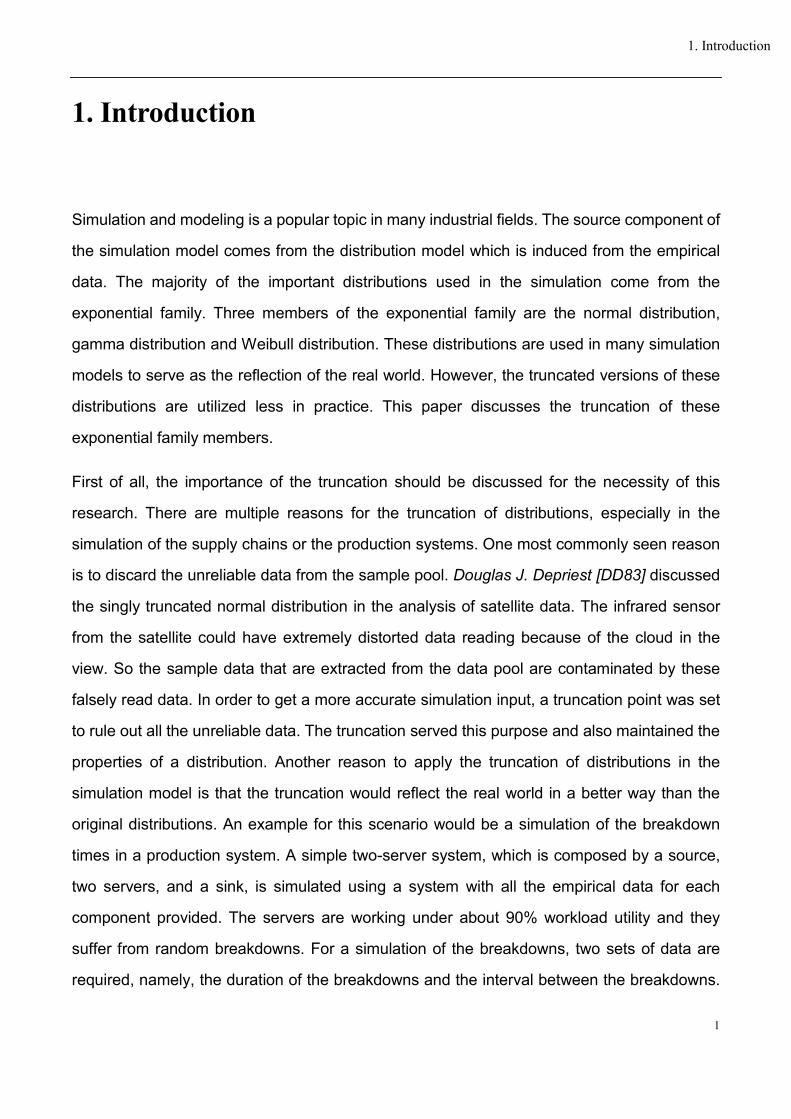
The standard form is denoted as

2

21

( )2

x

x e

. The figure of the normal distribution is

shown in Figure 2.1 [KC74].

Figure 2.1 Normal distribution density function

This is the normal distribution which is defined on the real numbers. Now the truncated

version of normal distribution is considered, which is a distribution defined on ( , )a b , instead

of on ( , ) . The probability density distribution (PDF) of truncated normal distribution

takes on the same form as the original one. The only modification here is the normalizing

constant, as discussed above. The probability of X falling into ( , )a b is

b a

P a x b

. Here ( )x indicates the cumulative probability of

normal distribution. 2 /21

( ) ( )2

x xtx t dt e dt

. The standardization of normal

distribution could be achieved using this substitution: 'x

x

[KC74].

8


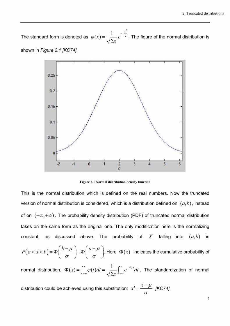
So the CDF of the truncated normal distribution defined on ( , )a b has the following form

[JK70]:

1

, ,

x

f x a bb a

(2.6)

The figure of the truncated normal distribution is shown in Figure 2.2. Note that with b=

and a= , the formula is (( ) / )b =1 and (( ) / )a =0

Figure 2.2 Truncated normal distribution

Now the left truncated normal distribution is considered, which means the defined area is now

a=truncation point t, b= . In this case, the above PDF is

1

( , )

1

x

f x tt

(2.7)

For a given sample X = ( 1 2, ,..., nx x x ), the log likelihood function of the left truncated normal

distribution is [AC50a]:

9


2

21

( ; ) log[ ( ; )] log 1 log 2 log2 2

ni

i

xt nl x L x n n

(2.8)

The parameters that need to be estimated in this function are and . After differentiating

the above log likelihood function with respect to and , the results are [DD83]:

2

2

2

2

2

2

( )2

2

( )1 1

2

2 2

1 1

( )

21

( )

2

( ) ( ) ( )2

( ) ( ) ( )4 0

( )

( )

t

n ni i

ti ir

n ni i

i i

nt i

i

t

r

x t e t t x t

n n

e dr

t x t x t

n n

x t

ne t

e dr

(2.9)

By solving this non-linear function system, the estimated parameter of interest: and

could be calculated.

2.3 Truncated Gamma distributions

The three parameter gamma distribution (as shown in Figure 2.3) has the following

probability density function:

( )1( )

( , , , ) , 0, 0, 0( )

x ca b

a

x c ef x a b c a b x c

b a

(2.10)

10


The standard gamma distribution has the following expression [JK70]:

1

( , ) , 0( )

a xx ef x a x

a

(2.11)

Figure 2.3 Gamma distribution

The truncated gamma distribution, especially the right truncated Weibull distribution, is

always used in the life-testing models. Douglas Chapman already discussed the estimation

of parameters from a truncated gamma distribution. Fisher gave the maximum likelihood

estimation equations L of the gamma distribution based on n samples [RF22]:

1

1

/ ( ) 0

1 ( ) 1ln ln( ) 0

( )

1 1 10

i

n

ii

n

i i

Lnb a x nc

a

L ba x c

n b b n

L ba

n c n x c

(2.12)

11


When the truncation point is known, which means, the distribution is now limited to a certain

truncation point T (T stands for the right truncation point) instead of . The probability

density function of a right truncated gamma distribution has the following expression [DC56]:

1 1( , , ) , 0, 0, 0ax bf x a b K e x a b T x

1

0( , )

Tax bK a b e x dx (2.13)

Also the moment method A. C. Cohen Jr. discussed in the truncated Pearson distribution

could also be used in the truncated gamma distribution [AC51].

2.4 Truncated Weibull distributions

The truncated distribution for different distribution families couldn’t be induced to a universal

form. Another member of the exponential distribution family is the Weibull distribution. Since

the three-parameter Weibull distribution could be transformed into other distributions when

replace certain parameters with a constant. Robert P. McEwen, Bernard R. Parresol [RB91]

discussed the moment expressions and summary statistics for the complete and truncated

Weibull distribution in details, as shown in some formulae of the following chapter. To make

the calculation easier, the explicit forms of the statistics of truncated Weibull distribution are

used. The moment expressions are needed here for inducing the explicit forms. The concept

of the moment was introduced from physics. The r-th moment of a real-valued function f(x) of

a real variable about a value c is

r

r x c f x dx

(2.14)

The r-th central moments of a probability distribution function is

r

r E X

The r-th non-central moments of a PDF of a continuous variable x is

12


( )rr E X

The two-parameter Weibull distribution is

1

( , , )

cx

b

cc x

f x b c eb b

， 0, 0, 0x b c (2.15)

where b is the scale parameter and c is the shape parameter.

The three-parameter Weibull distribution is [BSK62]:

1

( , , , ) , , 0, 0, 0

cx ac

bx acf x a b c e x a a b c

b b

(2.16)

where a is the location parameter, b is the scale parameter and c is the shape parameter.

The standard form of Weibull distribution is f(x,0,1,c) , as shown in Figure 2.4, where it could

be simply transformed to the three-parameter form by replacing x with 'x a bx .

Figure 2.4 Weibull distribution

The gamma function and the incomplete gamma function are needed to express the k-th

non-central moment of the truncated distributions. The gamma function ( )x is [KB00]:

13


1

0( ) x ux u e du

0x (2.17)

The normalized incomplete gamma function ( , )x r is [AS72]:

1

0( , )

rx ux r u e du 0n (2.18)

The left truncated three-parameter Weibull distribution is

1

( , , , ) exp

,0 , 0, 0

c cct a x ac x a

f x a b cb b b b

x t a t b c

(2.19)

The k-th non-central moment is [RB91]:

0

' exp 1,

c ck

k n nk

n

kt a k n t ab a

nb c b

(2.20)

The right truncated three-parameter Weibull distribution is

1

, , ,

1

, 0, 0, 0

c

c

x ac

b

T a

b

x ace

b bf x a b c

e

a x T a b c

(2.21)


0

1' 1,

1

c

ck

k n nk

T an

b

k k n t ab a

n c be

(2.22)

The doubly truncated three-parameter Weibull distribution is [RB91]:

14


1

, ( , , , )

1

, , 0, 0

c c

c

t a x ac

b b

t TT a

b

x ace

b bf x a b c

e

t x T a t b c

(2.23)


0

' 1, 1,

1

c

c

t ac cb k

k n nk

T an

b

k k n T a k n t aeb a

n c b c be

(2.24)

The reason why the k-th moments are introduced here is that the moments to calculate the

summary statistics could be used [PFTV92].

Mean: 1 'E X

Variance: 22 1' 'Var X

Skewness:

33 2 1 1

1 3/222 1

' 3 ' ' 2 '

' '

Kurtosis:

2 44 3 1 2 1 1

2 222 1

' 4 ' ' 6 ' ' 3 '

' '

(2.25)

Complete Weibull [RB91]

Mean: 1

1E X b ac

Variance: 2

2 2 11 1Var X b b

c c

(2.26)

15


Left truncated Weibull [RB91]

Mean:

11,

ct a c

b t aE X e b

c b

(2.27)

Variance:

2

2 2 11, 1,

cc t at a c cbb t a t a

Var X e b e bc b c b

(2.28)

Right truncated Weibull [RB91]

Mean:

1 11,

1

c

c

T a

b

T aE X b

c be

Variance:

2

21 2 1 11, 1,

1 1

c c

c c

T a T a

b b

T a T aVar X b b

c b c be e

(2.29)

Doubly truncated Weibull [RB91]

Mean:

/

1 11, 1,

11, 1,

c

c

c c

t a

b

c cT a b

T a t ab b

c b c beE X

e T a t aa a

b b

16


Variance:

2

2

2 21, 1,

1 12 1, 1,

1

1, 1,

c

cT a

b

c c

t ac cb

c c

T a t ab

c b c b

T a t aeVar X ba

c b c be

T a t aa

b b

2

1 11, 1,

1 1, 1,

c

cT a

b

c c

t a

b

c c

T a t ab b

c b c be

T a t ae a a

b b

(2.30)

17

3. Fitting of truncated Weibull distributions

This chapter deals with the fitting of truncated Weibull distributions into the raw data obtained

from real life. When a set of samples is already chosen, the underlying type of distribution is

determined with criteria like chi-square test or Kolmogorov-Smirnov test.

3.1 Fitting of Weibull distribution

A sample of data is drawn directly from the book written by Law and Merrill[AL00]. The raw

data contains 113 samples. Please note that due to the truncation, the sample size for the

truncated versions of Weibull distribution may vary.

Figure 3.1 shows the fitting of some distributions. Weibull distribution is considered to be the

one that best fits the data because of the Chi-Square test and Kolmogorov-Smirnov Test.

Figure 3.1 Histogram and distributions


18


The Weibull probability density function is

1.570.57 ( 0.1002 )( ) 0.1573 xf x x e (3.1)

And the Weibull cumulative density function is

1.57( 0.1002 )( ) 1 xF x e (3.2)

However, due to the accuracy of the measurement and the sampling method of the raw data,

some data needs to be discarded to improve the reliability of the fitting. The truncation points

will be given in the following chapter.

3.2 The fitting of truncated Weibull distributions

3.2.1 Fitting of left Weibull distribution

As seen above, the Weibull is the best fit of the sample. Now the focus is the fitting of

left-truncated Weibull distribution. Since some of the data are truncated, the sample size has

also changed with different truncation points.

The probability density function of left truncated Weibull distribution:

1

( , , , ) exp

c cct a x ac x a

f x a b cb b b b

(3.3)

For a more convenient calculation and the differentiation, the above expression is

transformed into another expression with 0a , 1/ '' bb a , 'c b . After the transformation

and taking out the apostrophe, a generalized form of probability density function of left

truncated Weibull distribution is solved [DRW89].

( )1( , , , )b bat axbf x a b t abx e (3.4)

The cumulative probability function is

19


( )( , , , ) 1b bat axF x a b t e (3.5)

With a sample of x, the log likelihood function of the sample is [DRW89]

( , , ) log log ( 1) log ( )b bi i iL a b x n a n b b x a x t (3.6)

To find the maximum likelihood estimates of the parameters, the global maximum of the

above LLF is differentiated into these two functions [DRW89]:

1

1 1

/ ( )

/ log ( log log )

nb b

ii

n nb b

i i ii i

Ln a x t

a

Ln b x a x x t t

b

(3.7)

The sum notations in the later chapters are all simplified from 1

n

i to , since the index

is always from 1 to the sample size.

After the substitution of the parameters, the functions are:

111( 0.5 ) 0

111log ( log 0.5 log0.5) 0

b bi

b bi i i

xa

x a x xb

(3.8)

By solving the above non-linear equation system, estimated parameters a and b could be

induced. After the calculation, the sample data could be fitted in a LTWD with the truncation

point chosen as t = 0.5 and the parameters:

0.109

1.5338

a

b

Now the LTWD probability density function with t = 0.5 is

1.53380.5338 (0.0376 0.109 )( ) 0.1672 xf x x e (3.9)

20


And the LTWD cumulative density function with t = 0.5 is

1.5338(0.0376 0.109 )( ) 1 xF x e (3.10)

3.2.2 Fitting of right truncated Weibull distribution

The right truncated Weibull distribution (RTWD) has the following probability density function

[DRW89]:

1 ( )

( )( , , , )

1

b

b

b ax

aT

abx ef x a b T

e

(3.11)

The cumulative RTWD probability function is [DRW89]

1( , , , )

1

b

b

ax

aT

eF x a b T

e

(3.12)

where T is the right truncation point. The log-likelihood function of the RTWD has the

following form [DRW89]:

( , , ) log log ( 1) log log[1 exp( )]b bi i iL a b x n a n b b x ax n aT (3.13)


above LLF is differentiated into these two functions [DRW89]:

exp( )

1 exp( )

log( ) exp( )log log

1 exp( )

b bb

i b

b bb

i i i b

L n nT aTx

a a aT

L n na T T aTx a x x

b b aT

(3.14)


112 12 exp( 12 )1120

1 exp( 12 )

112 log(12)12 exp( 12 )112log log 0

1 exp( 12 )

b b

bi b

b b

bi i i b

ax

a a

a ax a x x

b a

(3.15)

21



induced. After the calculation, the sample data could be fitted in a RTWD with the truncation

point chosen as T=12 and the parameters:

0.0915

1.6517

a

b

The RTWD probability density function converts to

1.65170.6517 ( 0.0915 )( ) 0.1517 xf x x e (3.16)

And the RTWD cumulative density function with T = 12 is

1.65170.09151( )

0.9961

xeF x

(3.17)

3.2.3 Fitting of doubly truncated Weibull distribution

The doubly truncated Weibull distribution (DTWD) has the following probability density

function:

1 ( )

( )( , , , , )

1

b b

b

b at ax

aT

abx ef x a b t T

e

(3.18)

The cumulative DTWD probability function is

( )

( )

1( , , , , )

1

b b

b

at ax

aT

eF x a b t T

e

(3.19)

where t and T are left and right truncation points respectively.

The log-likelihood function of the DTWD has the following form:

( , , ) log log ( 1) log ( )

log[1 exp( )]

b bi i i

b

L a b x n a n b b x a x t

n aT

(3.20)

After differentiation of the above LLF with respect to a and b, the functions are:

22


exp( )( )

1 exp( )

log( ) exp( )log ( log log )

1 exp( )

b bb

i b

b bb b

i b

b

i i

L n nT aTx

a a aT

L n na T T aTx a x x t t

b b aT

t

(3.21)


110 12 exp( 12 )110( ) 0

1 exp( 12 )

110 log(12)12 exp( 12 )110log ( log

0.5

0.5 log0.5) 01 exp( 12 )

b b

bi b

b b

b bi b

b

i i

ax

a a

a ax a x x

b a

(3.22)

With the truncation points t = 0.5, T = 12, the parameters of DTWD are:

0.0948

1.6384

a

b

The DTWD which fits this sample is:

1.63840.6384 (0.0305 0.0915 )( ) 0.1559 xf x x e (3.23)

And the DTWD cumulative density function with t = 0.5 and T = 12 is

1.6384(0.0305 0.0948 )1( )

0.9961

xeF x

(3.24)

Scale parameter Shape parameter

Weibull 0.1001 1.572

LT Weibull 0.109 1.5338

RT Weibull 0.0915 1.6517

DT Weibull 0.0948 1.6384

Table 3.1 Shape and scale parameters

23


Figure 3.2 Histogram and probability density distributions

Figure 3.3 Histogram and cumulative probability distributions

24


The truncated versions of the Weibull distribution possess the similar properties as the

original Weibull distribution. The shape and scale parameters of these parameters differ

slightly from each other, as shown above in Table 3.1.

The histogram and the fitted distributions are put in the above graphs to see the difference

between these alternatives. It could be observed that the shape of all the probability functions

and the cumulative probability functions show some difference between each other. In the

next chapters, the impact they have on the system performance when integrated in the

production systems are discussed and analyzed.

3.3 The truncation of the distribution

There are multiple reasons why the truncation of the distribution should be applied to the

simulation. The idea of the distribution truncation started quite early in the industrial practice.

In a production system, some intrinsic property of a distribution might lead to an inappropriate

result of the simulation. In these cases, the simulation calls for a truncation on the distribution

for a better interpretation of the reality. Some of the approaches for the truncation techniques

are discussed in the following passage.

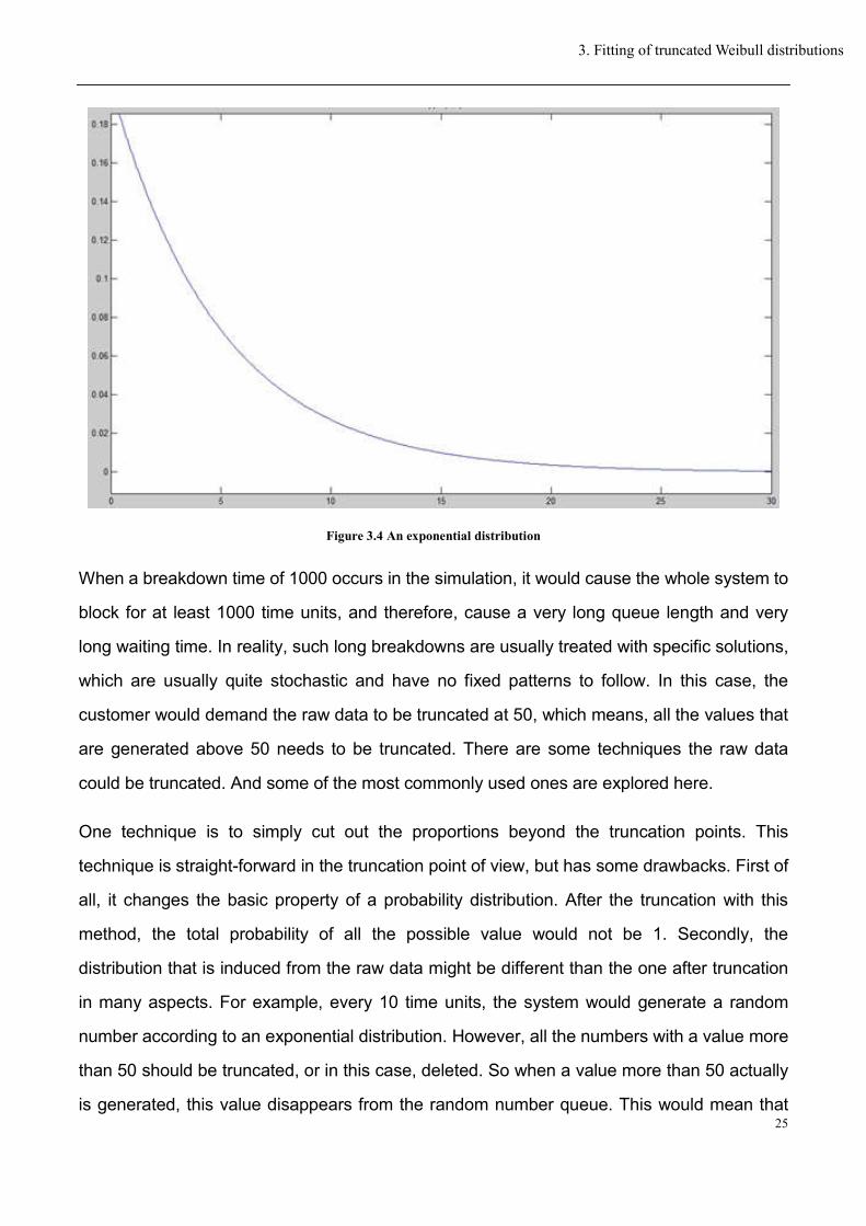
When a production system or a service system is simulated, some breakdown periods should

be considered. One most commonly used distribution for the breakdowns in the production

system is the exponential distribution, as shown in Figure 3.4.

It could be observed that even with a very small probability, some large value would still occur

no matter how “unlikely” that event might be. So in this case, some quite large breakdown

times would still happen during a long enough simulation time.

25


Figure 3.4 An exponential distribution

When a breakdown time of 1000 occurs in the simulation, it would cause the whole system to

block for at least 1000 time units, and therefore, cause a very long queue length and very

long waiting time. In reality, such long breakdowns are usually treated with specific solutions,

which are usually quite stochastic and have no fixed patterns to follow. In this case, the

customer would demand the raw data to be truncated at 50, which means, all the values that

are generated above 50 needs to be truncated. There are some techniques the raw data

could be truncated. And some of the most commonly used ones are explored here.

One technique is to simply cut out the proportions beyond the truncation points. This

technique is straight-forward in the truncation point of view, but has some drawbacks. First of

all, it changes the basic property of a probability distribution. After the truncation with this

method, the total probability of all the possible value would not be 1. Secondly, the

distribution that is induced from the raw data might be different than the one after truncation

in many aspects. For example, every 10 time units, the system would generate a random

number according to an exponential distribution. However, all the numbers with a value more

than 50 should be truncated, or in this case, deleted. So when a value more than 50 actually

is generated, this value disappears from the random number queue. This would mean that

26


the inter-generation time is at least 20 time units. This changes the behavior of the system

and would lead to a biased result.

To avoid the first disadvantage, another commonly used technique is to replace all the data

that are beyond the truncation points with the truncation points that are near them. In the

above example, the simulation treats any value that is higher than 50 to be the truncation

point, namely, 50. This technique could effectively truncate the data; however, it would also

cause a problem of an unexpectedly high probability at the truncation point. This truncation

has its obvious disadvantage, which is, it deprives the probability of its original property.

Although this does relieve the system by truncating all the points above 50, it still adds an

unusual high proportion of long breakdown time to the system.

The maximum likelihood method is the one used for the distribution fitting. This method could

effectively store the intrinsic property of the distribution and keep the basic property of a

probability density function. The mean-variance method could also be used for the fitting of

distribution from the raw data. This method might seem primitive on the first sight but it is also

robust when combined with the maximum likelihood estimation method.

The technique that is used later in this dissertation is the combination of the maximum

likelihood estimation method and the mean-variance method. This combination of these two

commonly used methods would restore the property of the distribution and keep the

parameters at its original level.

27

4. Truncated distributions in production systems

Although the difference in parameters is not obvious, the effect of the truncation would be

shown in the simulation. Here a simple model with two servers is introduced as an example.

To illustrate the effect of the different distributions on the model, two sets of comparison

simulations are made with all the distributions at source and distributions at the servers.

Before moving on to the numerical results section, an effective variation reduction technique

adopted in the simulation should be explained briefly. Common Random Number (CRN)

[AL07] is a technique which uses exactly the same stream of random numbers when

comparing alternate model configurations. Put simply, the same stream of random numbers

in the system gives all the alternatives the same condition. Moreover, the same random seed

is used in different random number generations of all the distributions. This guarantees that

the only reason that would lead to the difference in the final result is the distribution itself.

4.1 The M/Tr/1 queueing systems

If a queueing system consists in a source with an exponentially distributed inter-arrival time,

one server with a generally distributed service time, this system is denoted as an M/G/1

system. Denote the average rate of customers as , the average rate of service station as

, the service rate as / , the mean waiting time as W, and the mean number of

customers in the system as L, then the following equation holds [RC81]:

L W (4.1)

The above equation is also known as Little’s Theorem or Little’s formula.

For an M/G/1 system, the length of the system is as follows [GH98]:

2 2 2

2(1 )sL

(4.2)


28


where 2s is the variance of the service time. This equation is also referred to as the

Pollaczek - Khintchine (PK) formula. With the above formula the expected waiting time in the

queue could also be calculated [HT91]:

[ ] [ ] /E T E L (4.3)

For an M/Tr/1 system, the specifics are listed as follows:

The expected waiting time [RC812]:

21

1 2 2sW

(4.4)

The expected system length [PHB93]:

2 2 2

2(1 )sL

(4.5)

The expected queue length [PHB93]:

2 2 2

2(1 )s

qL

(4.6)

Before moving on to the next step, a test run of the simulation model is firstly taken to see if

the simulation results and the theoretical results match. The model is designed as the

following graph:

For the service station, it follows the Weibull distribution with a mean of 3.89 and a standard

deviation of 2.57.

The Weibull probability density function is

1.570.57 ( 0.1002 )( ) 0.1573 xf x x e (4.7)

And the Weibull cumulative density function is

29


1.57( 0.1002 )( ) 1 xF x e (4.8)

Figure 4.1 An example of a simple model

When the above model is run for 1000000 time units (tu), we have the average queue length

of 4.1074. The theoretical value of the average queue length is 4.1093. The expected waiting

time is wt =18.4088[tu] when we read directly from the simulation results, while the theoretical

value of average waiting time is 18.4238[tu]. Other alternative distributions are chosen to test

the model consistency. If the left truncated Weibull distribution using the mean and variance

method with the truncation point at t = 0.5 is chosen, the average queue length is 4.0994. The

theoretical value of the average queue length is 4.0839. The expected waiting time is

18.3732[tu] when read directly from the simulation results, while the theoretical value of

average waiting time is 18.3100[tu]. The next truncated distribution is the doubly truncated

Weibull distribution using the mean variance method and the maximum likelihood estimation

method. The simulation results show the average queue length is 4.1291 and the theoretical

value of the expected queue length is 4.0694. The average waiting time read from the model

results is 18.5065[tu]. The waiting time calculated from the formula is 18.2447[tu]. If the

model is run for 10000000 time units, the results of the scenario with the doubly truncated

Weibull distribution using the mean variance method and the maximum likelihood estimation

method show that the average queue length is 3.9587 and the average waiting time is

17.7755[tu]. The theoretical values are 3.99 and 17.9169[tu] respectively.

30


4.2 Truncated Weibull distributions as sources

4.2.1 Production systems without server breakdowns

The layout of the model is shown in the following figure:

Figure 4.2 Comparison of WD and TWD

Firstly, we compare the effect of the different distributions as source on the model. The only

modification we made in each round is the random number generation method (but still with

the same seed). A simulation of 100000 time units is made for each alternative. The results of

interest are the average waiting time (AWT) of both queues, the average queue length (AQL)

of both queues, average dwelling time (ADT) in both servers, the Utilization (Ut) of both

servers, the intergeneration time (IT), and the throughput (TP). The first round of simulation is

made under the condition that the queue capacity is infinite.

This result has a significant sense in the fact that the intergeneration time in this table reflects

the means of each distribution. From this table, we could see that the means of these

alternatives are different from each other. The means of the LTWD is the highest of all, while

the RTWD is the lowest. The DTWD is the closest to the original Weibull distribution. The

31


average queue length and the average waiting time is another important aspect of the model.

The reason why the queue length of RTWD is higher than the other alternatives lies not only

in the fact that the means of RTWD intergeneration time is the lowest. We take the first queue

as an example. The queue length before the first server is dependant on two factors: the

state of the server and the state of the arrival station. The server time obeys the exponential

distribution with the means of 3.46, as shown in the ADT S1. So the decisive aspect of the

queue length is the inter-arrival time of the source. There are two factors in the inter-arrival

time: the relieving factor and the aggravating factor. If the intergeneration time is extremely

small, this would put an aggravation to the waiting line. On the other hand, the large

inter-arrival time is a relief to the waiting queue since it gives the system more time to digest

the block in the queue. These two factors are the main reason of the difference in the above

table.

Weibull distributions as Sources / QC=infinite

parameters\distributions Weibull LTWD 0.5 RTWD 12 DTWD 0.5 12

IT 3.8805 3.962 3.8113 3.8495912

AWT Q1 20.336 16.115 23.557 19.222669

AQL Q1 5.2404 4.0669 6.1951 4.9927802

ADT S1 3.4646 3.4625 3.4699 3.4642568

Ut S1 0.8928 0.8738 0.909 0.8997541

AWT Q2 26.587 23.525 31.918 28.620898

AQL Q2 6.8505 5.9365 8.3599 7.4329963

ADT S2 3.5011 3.5043 3.4993 3.4991884

Ut S2 0.9021 0.8841 0.9164 0.908554

TP 25765 25229 26188 25963

Table 4.1 Weibull distribution as Sources with infinite QC

The LTWD takes out the aggravating factor in Weibull distribution. So the average waiting

time and average queue length of the first queue in LTWD model is the lowest. This is the

reason why the inter-generation time is about 2 percent higher than the original Weibull, but

the AWT and AQL in the first queue are 20 and 22 percent lower than those of Weibull. The

later section of this dissertation will also show that the left truncation not only takes out the

aggravating factor but also gives an increase to the relieving factor. So the LTWD still takes

on a Weibull form but with different properties.

32


Similar to the LTWD, the RTWD takes out the relieving factor of Weibull distribution. Its

inter-generation time is 1.78 percent lower, but the AWT and AQL in the first queue are 15

and 18 percent higher than those of Weibull.

The DTWD takes out both the relieving factor and the aggravating factor, which leads to a

relatively equivalent performance to the original Weibull distribution, only 5.5 and 4.7 percent

lower than the Weibull in average waiting time and average queue length.

As we can see from Table 4.1, the length of the queue follows the same order of the average

queue length and waiting time. But a capacity of 60 is too high for a real buffer size. So the

next round we make a simulation with the only modification of buffer size from infinite to 30.

Weibull distributions as Sources / QC=30


IT 3.8924 3.9441 3.7973 3.8470161

AWT Q1 18.296 17.061 25.67 20.147517

AQL Q1 4.6999 4.3255 6.7589 5.236194

ADT S1 3.4668 3.4689 3.494 3.4790597

Ut S1 0.8904 0.8794 0.9198 0.9041055

AWT Q2 23.989 22.418 31.137 27.978177

AQL Q2 6.1608 5.6836 8.1967 7.2702062

ADT S2 3.5012 3.5027 3.4979 3.4987212

Ut S2 0.8992 0.888 0.9208 0.9091137

TP 25680 25351 26322 25984

Table 4.2 Weibull distribution as Sources with QC=30

The result above shows the effect of the changes made in the queue capacity. The drastic

reduction in the average queue length and waiting time is an obvious effect of the capacity.

But this does not mean the improvement of the system performance. The capacity restricts

the length and the hence the waiting time. This time the LTWD has less effect on the

reduction of waiting time and queue length compared to Weibull distribution, 6.7 and 8.0

percent respectively. On the contrary, the RTWD has a much greater impact on system,

causing 40.3 and 40.8 percent more average waiting time and queue length than does the

original Weibull. For DTWD, the case has changed. In average waiting time and average

queue length, it changed from a reduction of 5.5 and 4.7 percent to an increase of 10.1 and

11.4 percent. The reason for this change lies in the fact that the restriction on the queue

33


capacity works as an aggravating factor on the model. The capacitated queue could cause

blocking in both directions. In the first round of simulation, there are times when the queue

length could go as high as 60. If this happens to a capacitated queue, a long period of

blocking could be expected. And this blocking to the server as well as to the source is the

main reason of the increase in the waiting percentage and the worse performance of the

system.

The last two rounds of simulation render an impression that the capacity of the queue length

makes a great change in the system performance. And more importantly, it also has

influence on the effects of truncated Weibull distributions. For the third round, a more realistic

queue capacity size is given to the system. This time, our interest is what 10 buffer size of the

waiting line could cause to that model.

Weibull distributions as Sources / QC=10


IT 3.9999 4.0708 3.9337 3.9675687

AWT Q1 15.833 13.873 17.393 16.303329

AQL Q1 3.9581 3.4074 4.4214 4.1085254

ADT S1 3.6304 3.6049 3.6577 3.6420007

Ut S1 0.9076 0.8852 0.9298 0.9176814

AWT Q2 14.887 14.1 16.096 15.509006

AQL Q2 3.7211 3.4626 4.0914 3.9077889

ADT S2 3.5026 3.5035 3.504 3.5039443

Ut S2 0.8754 0.8602 0.8904 0.8825399

TP 24992 24549 25410 25187

Table 4.3 Weibull distribution as Sources with QC=10

This result confirms that the capacity of the waiting line does play an aggravating role in the

system. Although in this time, all the four alternatives are dramatically restricted by this

capacitating that the effects of the truncation at the source are not so obvious.

4.2.2 Production systems with server breakdowns

These three rounds of simulation illustrate the relieving factor and the aggravating factor of a

system and their relationship with the truncation of Weibull distribution at the source. Like the

capacity of the waiting line, another aggravating factor of the system is the breakdown of the

34


server. This time we are interested in the effect of this aggravating factor. A breakdown

module and warm-up phase after the breakdown is added to the model.

After the addition of the breakdown—repair—warm-up module, a model with 30 as queue

capacity is simulated for 100000 time units. The table below lists the result of the simulation:

Weibull distributions as Sources / QC=30 with breakdown


IT 4.0245 4.0515 3.9994 4.0088686

AWT Q1 65.17 55.521 86.423 76.447166

AQL Q1 16.195 13.703 21.598 19.063259

ADT S1 3.5932 3.5664 3.6214 3.6132663

Ut S1 0.8917 0.8793 0.9044 0.9006802

AWT Q2 61.321 54.802 66.366 62.943388

AQL Q2 15.216 13.51 16.574 15.685513

ADT S2 3.5042 3.504 3.5026 3.5028737

Ut S2 0.8695 0.8638 0.8747 0.8728847

TP 24812 24650 24972 24918

Table 4.4 Weibull distribution as Sources with QC=30 with breakdowns

As shown in the table above, the breakdown of the server has a significant impact on the

system performance. The average waiting time and average queue length of the first queue

of the Weibull distribution generated system with a breakdown are as high as 356.2% and

344.6% of the one without a breakdown, respectively. For the models that are generated by

the left truncated Weibull and right truncated Weibull distribution, the impact of the

breakdown is relatively less as the breakdown works as a variance-absorbing factor of the

system. It diminishes other factors made on the system to some extent. Therefore, even if the

truncated distribution could still make a difference on the system, their roles in the system

performance are relatively less when the servers come across with breakdowns.

To illustrate the difference between the original Weibull distribution and the truncated version,

we take another more extreme case where the left truncation point is chosen to be 1. The

choice of the truncation point can be significant in fitting the sample to a distribution. The left

truncation point should be set to less than 0.5 in this case. An extreme truncation point would

only lead to an extreme outcome. Now we illustrate the consequences caused by this choice.

First we calculate the parameter estimation of the left truncated Weibull distribution at t = 1.0.

35



above LLF is differentiated into these two functions:

/ ( )

/ log ( log log )

b bi

b bi i i

Ln a x t

a

Ln b x a x x t t

b

(4.9)

After the substitution of the parameters, we have:

102( 1) 0

102log ( log ) 0

bi

bi i i

xa

x a x xb

(4.10)


induced. After the calculation, the sample data could be fitted in a LTWD with the truncation

point chosen as t = 1.0 and the parameters:

0.09

1.57

a

b


1.570.57 (0.09 0.109 )( ) 0.1413 xf x x e (4.11)


1.57(0.09 0.09 )( ) 1 xF x e (4.12)

Two scenarios are presented to compare the effect of choosing 1 to be the truncation point:

infinite queue capacity without breakdown, and queue capacity of 30 with breakdown.

36


Weibull distributions as Sources / QC=infinite no breakdown

parameters\distributions Weibull LTWD 0.5 LTWD 1

IT 3.88046 3.96201 4.50271

AWT Q1 20.3359 16.1147 7.21497

AQL Q1 5.24036 4.06691 1.6023

ADT S1 3.46461 3.46247 3.4731

Ut S1 0.89276 0.87382 0.77127

AWT Q2 26.5871 23.5249 10.0238

AQL Q2 6.85046 5.93655 2.22601

ADT S2 3.50111 3.50429 3.50311

Ut S2 0.90208 0.88411 0.77778

TP 25765 25229 22202


parameters\distributions Weibull LTWD 0.5 LTWD 1

IT 4.02449 4.05146 4.51047

AWT Q1 65.1696 55.5206 15.8061

AQL Q1 16.1951 13.7035 3.50395

ADT S1 3.59319 3.56643 3.47773

Ut S1 0.89175 0.87929 0.77091

AWT Q2 61.3207 54.8019 23.7317

AQL Q2 15.2158 13.5096 5.25988

ADT S2 3.50416 3.50399 3.5033

Ut S2 0.86946 0.86376 0.7761

TP 24812 24650 22153

Table 4.5 Weibull distribution as Sources with QC=inf and QC=30 with breakdowns

These two tables show the extreme relieving factor that the left truncation at 1.0 plays. In the

first scenario, the average waiting time and average queue length of the first queue has

dropped as much as 64.5% and 69.4 % respectively, compared to the model with original

Weibull distribution. This drastic change is the direct result of the fact that intergeneration

time with the left truncation is never lower than 1.0. This means that the system would always

have enough time to “digest” the lower and middle level congestion in the queue. Only the

severe congestion could cause the temporary block in the system. As a matter of fact, the

average waiting time in the first queue is just 1.6 time units, which indicates the majority of

the entities passes the system without having to wait or only have to wait for a small amount

of time.

37


Compared to the first scenario, the second one is more informative in showing the relief that

the left truncation would bring to the system. As discussed above, the breakdown of the

server is a great aggravating factor of the system. The average waiting time and average

queue length of the first queue of the Weibull distribution generated system with a breakdown

is as high as 356.2% and 344.6% of the system without a breakdown. But such a great

increase is not observed in the left truncation of 1.0. The maximum queue length of the left

truncated distribution at 1.0 with a queue of infinite capacity is 21. (The table of the maximum

queue length will be listed in later chapter.) So the queue capacity of 30 does not have an

effect on such a model. The average waiting time and average queue length of the left

truncated Weibull distribution at 1.0 system with a breakdown is just as high as 219% and

218% respectively. This means the relieving factor of left truncation at 1.0 is much greater

than the other relieving factors we mentioned.

Now we take another closer look at the probability density function and the cumulative

probability function of Weibull distribution, left truncated Weibull distribution at t = 0.5, right

truncated Weibull distribution at T = 12, double truncated Weibull distribution at t = 0.5 and T

= 12, and left truncated Weibull distribution at t = 1.0.

Figure 4.3 Histogram and probability density distributions

38


Figure 4.4 Histogram and cumulative probability distributions

It is shown in the first graph, that the Weibull distribution has more a ‘balanced’ distribution as

it is non-zero on both ends. The truncated versions, on the other hand, put more emphasis on

the middle part since either or both ends are truncated. It is clearly shown in the second

graph that the truncated version starts only at the truncated points. Also, in the first graph, the

tails of the probability density functions are different from one another. The tail of the left

truncated Weibull at t = 1.0 is higher than the other distributions, for the purpose of making up

the truncated part at the other end.

Along with the reduction on the queue length and waiting time, the throughput of the left

truncated Weibull distribution at t = 1.0 is also reduced to some extent. The main reason for

this change is the inter-generation time of the source. As shown in the table above, the

inter-generation time of the original Weibull distribution is 3.88 time units, while the

inter-generation time of the left truncated Weibull distribution at 1.0 is 4.5 time units. This

difference leads to the result that the system with the left truncated Weibull distribution would

generate fewer objects than the one with Weibull distribution in the same amount of time,

which is one of the reasons why the throughputs of these systems are different from each

other.

39


The above discussion gives us another viewpoint regarding the source of these different

systems. That is, the mean inter-generation time of the source also plays an important role in

the system performance. The following chapter is the truncation of Weibull distribution

focused on the mean time.

4.3 Alternative truncated distributions with M-V

The method to determine the parameters of a distribution was the maximum likelihood

estimation of the log-likelihood function. This time, the parameters are estimated by the mean

and variance (M-V) of the distributions and the data itself. The original Weibull distribution

has a mean of 3.8866 and a variance of 6.6296. These two numbers will be the focus of the

distribution fitting in this chapter.

4.3.1 Fitting of the truncated distribution with M-V

According to the mean and variance expressions of the complete and truncated Weibull

distribution, (2.27), (2.28), (2.29), and (2.30), the parameters of the truncated distributions

can be calculated.

First of all, the left truncated Weibull distribution with the truncation point at t = 0.5:

0.5 /

0.5 / 2

2

0.5 /

1

'

11, 0.5 / 3.8866

21, 0.5 /

11, 0.5 / 6.6296

0

'

'

c

c

c

ca b

ca b

ca b

b

e b a bc

e b a bc

e b a bc

a

b a

c b

(4.13)

40


The parameters we are interested in are a‘ and b‘. The result of the above function systems

is:

' 0.1330

' 1.4326

a

b


1.53380.4326 (0.0493 0.133 )( ) 0.1905 xf x x e (4.14)


1.4326(0.0493 0.133 )( ) 1 xF x e (4.15)

Next distribution to fit is the right truncated Weibull distribution at T = 12:

12 /

2

12 /

2

12 /

1

'

1 11, 12 / 3.8866

1

1 21, 12 /

1

1 11, 12 / 6.6296

1

0

'

'

c

c

c

c

a b

c

a b

c

a b

b

b a bce

b a bce

b a bce

a

b a

c b

(4.16)

The parameters we are interested in are a‘ and b’. The result of the above function systems

is:

' 0.1158

' 1.4436

a

b

The RTWD probability density function at T = 12 is

41


1.44360.4436 ( 0.1158 )( ) 0.1697 xf x x e (4.17)

And the RTWD cumulative density function with T=12 is

1.4436( 0.1158 )1( )

0.9848

xeF x

(4.18)

Then we move on to the doubly truncated Weibull distribution at t = 0.5 and T = 12.

1

'

0.5 /

12 /

2

0.5 /

12 /

0

'

1 11, 12 / 1, 0.5 /

3.88661 1, 12 / 1, 0.5 /

2 21, 12 / 1, 0.5 /

12 1, 12 /

1

c

c

c

c

b

c ca b

a b c c

c c

a b

a b

a

b a

b a b b a be c c

e a a b a a b

b a b a bc c

eba a

ce

2

2

0.5 /

12 /

11, 0.5 /

1, 12 / 1, 0.5 /

1 11, 12 / 1, 0.5 /

6.6296

1 1, 12 / 1, 0.5 /

c

c

c c

c c

c ca b

a b c c

b a bc

a a b a b

b a b b a be c c

e a a b a a b

'c b

(4.19)


is:

42


' 0.0908

' 1.6529

a

b

The probability density function of doubly truncated Weibull distribution which fits this sample

is:

1.65290.6529 ( 0.0908 0.0289)( ) 0.1507 xf x x e (4.20)

And the doubly truncated Weibull distribution cumulative density function with t = 0.5 and T =

12 is

1.6529(0.0289 0.0908 )1( )

0.996

xeF x

(4.21)

The last but not the least, the left truncated Weibull distribution with the truncation point at

t=1.0. This is the distribution that gives us the inspiration of fitting according to the mean and

variance.

1 /

1 / 2

2

1 /

1

'

11, 1 / 3.8866

21, 1 /

11, 1 / 6.6296

0

'

'

c

c

c

ca b

ca b

ca b

b

e b a bc

e b a bc

e b a bc

a

b a

c b

(4.22)


is:

' 0.299

' 1.4326

a

b

43


Now the LTWD probability density function with t = 1 is

1.06630.0663 (1 0.299 )( ) 0.3188 xf x x e (4.23)

And the LTWD cumulative density function with t = 1 is

1.0663(0.299 0.299 )( ) 1 xF x e (4.24)

A simple test is made to examine the mean of these newly generated truncated versions of

Weibull distribution. The following model shows both the trend and the result of the average

inter-generation time.

Figure 4.5 The model for testing

The block with the name “different distributions” are to be replaced by different truncated

distributions. The scope of average inter-generation time shows the trend and the display

block “result” shows the result of the inter-generation time. We run this model for enough long

time to examine the result of the distribution fitting.

Weibull distribution:

44


Figure 4.6 The results of Weibull Distribution

Left truncated Weibull distribution at t = 0.5:

Figure 4.7 The results of LT Weibull Distribution

Right truncated Weibull distribution at T = 12:

Figure 4.8 The results of RT Weibull Distribution

45


Doubly truncated Weibull distribution at t = 0.5 and T = 12:

Figure 4.9 The results of DT Weibull Distribution

Left truncated Weibull distribution at t = 1:

Figure 4.10 The results of LT Weibull at t=1 Distribution

The purpose of doing these tests is showing the inter-generation time of running the models

for enough long time units. In the later discussion, the models will not be run for such a long

time as the inter-generation time of each model might not be this close to each other. It could

be observed from these tests that these distributions have the mean and variance in common,

which means, the only reason that could lead to the different performance of the systems is

the distribution itself.

46


4.3.2 Implementing of the distributions into the model

Two rounds of simulation are made to compare the results of simulation: one with infinite

queue capacity and no breakdown and another with a queue capacity of 30 and with a

breakdown.

Firstly, the simulation with infinite queue capacity and no breakdown from the server blocks:

Weibull distributions as Sources / QC=inf no breakdown

parameters\distributions Weibull LTM 05 LTM1 RTM DTM

IT 3.88046 3.9167 3.92417 3.90594 3.89988

AWT Q1 20.3359 20.3065 19.2001 20.1371 19.5363

AQL Q1 5.24036 5.18435 4.89217 5.15479 5.00889

ADT S1 3.46461 3.46311 3.463 3.46451 3.46413

Ut S1 0.89276 0.88412 0.8823 0.88654 0.88811

AWT Q2 26.5871 25.292 24.6278 25.5626 25.7819

AQL Q2 6.85046 6.4559 6.27453 6.54078 6.60919

ADT S2 3.50111 3.50289 3.50281 3.50169 3.50253

Ut S2 0.90208 0.89405 0.89239 0.896 0.8977

TP 25765 25523 25476 25586 25630

Table 4.6 Weibull distribution as Sources with QC=inf no breakdown

Because the simulations are run for a certain amount of time units, the inter-generation time

are not all the same in the above table. As discussed earlier, it is just a matter of simulation

time. Despite the little difference in inter-generation times, the difference in the other

performance parameter of the systems seem to have been reduced a lot than the previous

distribution fitting. We could notice just slight difference in the average waiting time and

average queue length. Such resemblance could also be observed in the comparison run

where the queue has a capacity of 30 and the server suffers breakdown from time to time.

Table 4.7 shows that the average queue length and average waiting time of the queues are

merely slightly different from each other, e.g. the average waiting time of the first queue with

Weibull distribution is 65.2 time units while the one with right truncated Weibull distribution is

67.7 time units. However, this 4% increase is too small when compared to the 32.6% in the

previous fitting.

47




IT 4.02449 4.02645 4.02947 4.02186 4.02643

AWT Q1 65.1696 67.1205 67.3845 67.7411 65.2227

AQL Q1 16.1951 16.6741 16.7209 16.8413 16.1976

ADT S1 3.59319 3.57659 3.59654 3.60103 3.59187

Ut S1 0.89175 0.88716 0.89155 0.89424 0.89095

AWT Q2 61.3207 59.4225 61.6499 61.366 59.8817

AQL Q2 15.2158 14.7394 15.2784 15.2385 14.8533

ADT S2 3.50416 3.50392 3.50494 3.50392 3.50392

Ut S2 0.86946 0.86912 0.86853 0.87007 0.86912

TP 24812 24804 24780 24831 24804


Up until now, these results show no big difference between the original Weibull distribution

and the truncated versions. The reason that lies beneath is the fact that these two scenarios

“absorb” the effect of the truncations so no conspicuous distinction could be observed from

the results. The first scenario, where the system has infinite queue capacity and no

breakdown, is the one where the system has enough time to deal with the entities coming in

and even when the server suffered from blocking, the system still managed to get out of that

situation soon enough. So the average waiting time, the average queue length, the dwelling

time of the entities in each server and the throughput of the system are determined by the

mean of the distribution at the source. Since all these distributions share the same mean and

variance, the performance of the system in a long enough time interval is roughly the same.

The second scenario is on the opposite side of the situation. When the both servers suffer

from breakdowns from time to time, the whole system is in the “blocking” status as the

servers could not handle the incoming entities. And with a queue capacity limit, the system

enters a relatively “steady” state after the “warm-up” phase. This “steady state”, has almost

nothing to do with the shape and scale parameters of the source distribution. The only factor

that matters in the mean of the distribution. This is the reason why the performances of the

system under various sources under these two scenarios are almost the same. Next round of

simulation is made with unlimited queue capacity and breakdown of the servers.

48


Weibull distributions as Sources / QC=inf with breakdown


IT 3.90625 3.90277 3.898 3.91489 3.9008

AWT Q1 130.662 221.616 151.957 150.909 99.029

AQL Q1 33.4255 56.7287 38.9516 38.517 25.3818

ADT S1 3.46346 3.46457 3.46384 3.46308 3.46457

Ut S1 0.88539 0.88646 0.8871 0.88348 0.88646

AWT Q2 180.873 197.316 168.338 186.602 210.963

AQL Q2 46.2088 50.4735 43.0954 47.5654 54.1594

ADT S2 3.5034 3.5024 3.5033 3.50266 3.50346

Ut S2 0.89334 0.89374 0.89478 0.8922 0.89143

TP 25499 25517 25541 25472 25444

Table 4.8 Weibull distribution as Sources with QC=inf with breakdowns

In this round of simulation, although the inter-generation time of these distributions are almost

the same, the system performances of these alternatives are much different from each other.

The average waiting time and average queue length shows more distinction in this round of

simulation. The average queue length of the first queue in a system with left truncated

Weibull distribution at t = 0.5 is 170% as high as the one with Weibull distribution, and is

223.8% as high as the system with doubly truncated Weibull distribution. The reason why left

truncated Weibull distribution at t = 0.5 creates such a high rate of waiting time and queue

length is that the majority of the inter-generation time lies between the interval of [0.5 3.5],

and it doesn’t generate enough relieving numbers like the left truncated Weibull distribution at

t = 1.0. Plus, the two servers interact in a bad way that also leads to the blocking at the queue.

This is a list of the maximum queue length comparison between these alternatives.

The scenario when the servers suffer from breakdowns and when servers do not suffer from

breakdowns are listed in Table 4.9.

The second row in the following table shows that although the other performance results from

the models are not so different, but the maximum length of the queue still displays distinction

which reflects the system behavior in a way.

49


Maximum Queue Length

Infinite queue with breakdown Weibull LT05M LT1M RT12M DTM

134 207 159 146 98

Infinite queue without breakdown Weibull LT05M LT1M RT12M DTM

50 53 46 61 59

Table 4.9 Comparison of servers with and without breakdowns

The following graphs show the probability density function and the cumulative probability

function of Weibull distribution, left truncated Weibull distribution at 0.5, right truncated

Weibull distribution at 12, double truncated Weibull distribution at 0.5 and 12, and left

truncated Weibull distribution at 1.0. All of them have the same mean and variance.

Figure 4.11 The probability density functions of multiple distributions

The probability density functions of the distributions show the extreme case when the left

truncation point is chosen to be t = 1.0. The density function of this truncated Weibull

distribution has a non-increasing curve which is never seen in other cases. By using the

common random number technique, the simulation is done with the blocks from common

random number series. Also for the source block, the same seed of random number

generation is used to reduce the variation.

50


Figure 4.12 The cumulative probability functions of multiple distributions

The following table 4.10 is the starting points of each distribution. The left truncated functions

start at the corresponding truncation point. The right truncated Weibull distribution starts a

little lower than the original Weibull because the truncation changed the shape of the

probability density function. So it is pressed a little in the beginning.

Weibull LT05M RTM DTM LT1M

0.00856 0.5004 0.00501 0.50059 1.00018

0.02731 0.50246 0.01772 0.50362 1.00109

0.02732 0.50247 0.01773 0.50363 1.00109

0.03206 0.50317 0.0211 0.50466 1.00141

0.03729 0.50402 0.02487 0.50591 1.00178

Table 4.10 A breakdown of the multiple distributions step 1

It takes other distributions almost 1000 steps to reach the benchmark 1.0. And the distribution

that started at 1.0 is now 1.36, still the highest of all (as shown in step 2).

Although the left truncated distribution at t = 1.0 had a good start, it is caught on and

surpassed in a quite short time. It is the last one to reach 2.0. The left truncation distribution

at t = 0.5, which also had a good start, is the second to the last (as shown in step 3).

51



1.10661 1.16994 0.99745 1.33089 1.36383

1.10668 1.17 0.99752 1.33095 1.36387

1.10766 1.1708 0.99847 1.33185 1.36437

1.1108 1.17337 1.00156 1.33473 1.36598

1.11155 1.17398 1.0023 1.33542 1.36637



2.12424 2.06612 2.02644 2.27848 1.99922

2.12469 2.06654 2.02691 2.27891 1.99955

2.1247 2.06655 2.02692 2.27892 1.99956

2.12543 2.06723 2.02768 2.2796 2.00009

2.1262 2.06794 2.02847 2.28032 2.00064


By the time the doubly truncated distribution reaches 3.0, the two left truncated distributions

are left far behind.


2.89282 2.79676 2.83245 2.99706 2.60556

2.89387 2.79778 2.83356 2.99804 2.60645

2.89573 2.79959 2.83554 2.99978 2.60804

2.89699 2.80081 2.83687 3.00095 2.6091

2.89712 2.80093 2.837 3.00107 2.60921


Soon enough, the right truncated Weibull takes over the lead and first reaches 5 because of

the right truncation on the tail.


4.9014 4.82035 4.99678 4.85349 4.58264

4.90296 4.82197 4.99847 4.85492 4.58436

4.90423 4.82328 4.99985 4.85608 4.58576

4.90483 4.82391 5.0005 4.85663 4.58643

4.90757 4.82675 5.00349 4.85914 4.58947


52


To save the length of the paper, we jump directly to the end. It is shown that the right

truncated distributions end at the truncation point. The left truncated ones end with much

higher numbers, especially the left truncated distribution at t = 1.0.


15.4991 16.6606 11.9297 11.8599 21.125

15.8142 17.0301 11.9453 11.8966 21.7365

16.501 17.8383 11.9695 11.9543 23.0899

16.8623 18.2647 11.9781 11.9753 23.8127

16.9519 18.3706 11.9799 11.9797 23.9932


These moments illustrate the random number generation at the source block. Take the left

truncated distribution at t = 1.0 as an example: it starts with 1.0 while the others start at 0.5 or

0. This advantage at the beginning is certainly a relieving factor as it doesn’t generate entities

that come so close to each other. However, this advantage doesn’t last very long. Soon

enough, the left truncated distribution is the lowest of all. The reason for this change is the

distribution fitting criteria. In order for all the distributions to have the same mean and

variance, the left truncated distribution has to put more emphasis on the beginning part to

balance out the left truncation at a high value and the increase at the tail. Therefore, the

system with such a truncated distribution doesn’t have the best performance of all. On the

contrary, it is usually the worst one in most cases.

From what we discussed above, we may draw the conclusion that, using the mean and

variance as the criteria might not be the best way for distribution fitting. It focuses on the

global behavior of two parameters of the data and ignores the local properties and details. It

has the advantage of generating equally distributed random numbers, but the disadvantage

of losing subtlety is also a big drawback.

The first two rounds of the distribution fittings are based on two different criteria: the

maximum likelihood estimation, and the mean and variance. These two methods have their

own advantages and disadvantages. One natural idea would be to combine them together to

get the best out of these two methods. The following section deals with this combination.

53


4.3.3 Truncated distributions with MLE and M-V

When we combine the criteria of these two methods together, we have the two maximum

likelihood estimation (MLE) functions, and two functions about the mean and the variance

(M-V). So to utilize them to the fullest, not only the scale and shape parameters but also the

truncation point is considered to be the unknown element here.

The truncation point is no longer a constant before the simulation and the modeling, which

means, besides the maximum likelihood estimators, another one or two functions are needed

to determine the additional variable. For the left truncated and right truncated Weibull

distribution, we take the maximum likelihood estimators and the mean or variance of the

distribution. For the doubly truncated distribution, we need the mean and the variance as well

as the maximum likelihood estimators, because the doubly truncated distribution has two

truncation points to estimate.

Firstly, the calculation of the parameters is executed for each distribution. For the left

truncated Weibull distribution, the maximum likelihood estimators and the mean expression

are listed below.

/ ( )

/ log ( log log )

11,

c

b bi

b bi i i

t a c

b

Ln a x t

a

Ln b x a x x t t

b

t aE X e b

c b

(4.25)


54


' '

' '

1

'

113( ) 0

'

113log ' ( log log ) 0

'

11, 3.8866

0

'

'

c

b bi

b bi i i

t a c

b

b

x ta

x a x x t tb

t ae b

c b

a

b a

c b

(4.26)

The parameters of interest here are a’, b’, and t. By solving the above non-linear equation

system, estimated parameters a, b and the truncation point t could be induced. After the

calculation, the parameters of interest are:

' 0.1871

' 1.2721

0.7261

a

b

t

Now the left truncated Weibull probability density function with t = 0.7261 is

1.27210.2721 (0.1245 0.109 )( ) 0.2380 xf x x e (4.27)


1.2721(0.1245 0.1871 )( ) 1 xF x e (4.28)

The maximum likelihood estimators and the mean expression of the right truncated Weibull

distribution are listed below.

55


exp( )

1 exp( )

log( ) exp( )log log

1 exp( )

1 11,

1

c

b bb

i b

b bb

i i i b

c

T a

b

L n nT aTx

a a aT

L n na T T aTx a x x

b b aT

T aE X b

c be

(4.29)


' ''

'

' ''

'

1

'

113 113 exp( ' )0

' 1 exp( ' )

113 113 'log( ) exp( ' )log ' log 0

' 1 exp( ' )

1 11, 3.8866

1

0

'

'

c

b bb

i b

b bb

i i i b

c

T a

b

b

T a Tx

a a T

a T T a Tx a x x

b a T

T ab

c be

a

b a

c b

(4.30)

The parameters of interest here are a’, b’, and T. By solving the above non-linear equation

system, estimated parameters a’, b’, and T could be induced. After the calculation, the

parameters of interest are:

' 0.1017

' 1.5544

13.8653

a

b

T

The right truncated Weibull probability density function converts to

1.55440.5544 ( 0.1017 )( ) 0.1584 xf x x e (4.31)

56


And the RTWD cumulative density function with T = 13.8653 is

1.5544( 0.1017 )1( )

0.9977

xeF x

(4.32)

The maximum likelihood estimators, the mean expression, and the variance expression of

the right truncated Weibull distribution are listed below.

/

exp( )( )

1 exp( )

log( ) exp( )log ( log log )

1 exp( )

1 11, 1,

11,

c

c

b bb

i b

b bb b

i i i b

c c

t a

b

T a b

bL n nT aTx

a a aT

L n na T T aTx a x x t t

b b aT

T a t ab b

c b c beE X

e

t

T aa

b

2

1,

2 21, 1,

1 12 1, 1,

1

c

cT a

b

c c

c c

t ac cb

t aa

b

T a t ab

c b c b

T a t aeVar X ba

c b c be

2 1, 1,

1 11, 1,

1 1, 1

c

cT a

b

c c

c c

t a

b

c

T a t aa

b b

T a t ab b

c b c be

T ae a a

b

2

,

ct a

b

(4.33)

57


After the substitution of the parameters, we have the following non-linear equation system:

' ''

'

' ''

'

0.5 /

12 /

113 113 exp( ' )0

' 1 exp( ' )

113 113 'log( ) exp( ' )log ' log 0

' 1 exp( ' )

1 11, 12 / 1, 0.5 /

1 1, 12 / 1, 0.5 /

c

c

b bb

i b

b bb

i i i b

c ca b

a b c c

T a Tx

a a T

a T T a Tx a x x

b a T

b a b b a be c c

e a a b a a b

2

0.5 /

12 /

2

0.5 /

12 /

3.8866

2 21, 12 / 1, 0.5 /

1 12 1, 12 / 1, 0.5 /

1

1, 12 / 1, 0.5 /

1

c

c

c

c

c c

a bc c

a b

c c

a b

a b

b a b a bc c

eba a b a b

c ce

a a b a b

e

e

2

1

'

1 11, 12 / 1, 0.5 /

6.6296

1, 12 / 1, 0.5 /

0

'

'

c c

c c

b

b a b b a bc c

a a b a a b

a

b a

c b

(4.34)

The parameters of interest here are a’, b’, t and T. By solving the above non-linear equation

system, estimated parameters a’, b’, and T could be induced. After the calculation, the

parameters of interest are:

58


' 0.1082

' 1.5302

0.2120

16.1452

a

b

t

T

The doubly truncated Weibull density function which fits this sample is:

1.53020.5302 (0.0101 0.1082 )( ) 0.1657 xf x x e (4.35)

And the doubly truncated Weibull cumulative density function with t = 0.2120 and T = 16.1452

is

1.5302(0.0101 0.1082 )1( )

0.9995

xeF x

(4.36)

The truncation points that are calculated by this method are somehow questionable. For

example, the truncation point of the left truncated Weibull distribution is 0.7261. This point

might not be acceptable in some cases. If the lower limit of the data is close to the original

lower limit of the data, this truncation point should be discarded.

Weibull distributions as Sources / QC=30 with no breakdown

parameters\distributions Weibull LTMM RTMM DTMM

IT 3.89239 3.88474 3.89108 3.89395

AWT Q1 18.2961 21.0788 20.456 21.4812

AQL Q1 4.69986 5.42571 5.25619 5.51572

ADT S1 3.46677 3.47299 3.47396 3.48595

Ut S1 0.8904 0.89392 0.89246 0.89498

AWT Q2 23.989 26.4895 26.5048 26.8901

AQL Q2 6.16084 6.81686 6.80884 6.90324

ADT S2 3.50118 3.50183 3.50086 3.50141

Ut S2 0.89916 0.90095 0.89931 0.89886

TP 25680 25728 25688 25670

Table 4.16 Weibull distribution as Sources with QC=30 without breakdowns

However, all these truncation points are assumed to be acceptable here. To compare the

effect of truncation using maximum likelihood estimation and mean and variance, some

rounds of simulation are run with the same set of models except for the source block. Firstly,

59


two rounds of simulation where the queue has a capacity of 30 and with or without

breakdown are run.



IT 4.02449 4.02441 4.02778 4.01285

AWT Q1 65.1696 70.2513 66.7218 67.9145

AQL Q1 16.1951 17.4542 16.5631 16.9189

ADT S1 3.59319 3.61099 3.59069 3.60235

Ut S1 0.89175 0.89616 0.89039 0.89669

AWT Q2 61.3207 61.0748 59.7928 62.8361

AQL Q2 15.2158 15.1548 14.8261 15.6386

ADT S2 3.50416 3.50416 3.50432 3.50313

Ut S2 0.86946 0.86946 0.86889 0.87186

TP 24812 24812 24794 24885


It is shown in the above two tables that the inter-generation time of all these distributions are

almost the same, which is a result of controlling the mean of each alternative. The model with

a left truncation has the worst performance of all, as the ones with the previous distribution

fitting criteria. The queue capacity of 30 limits the effects of the truncation to an extent. The

source generates the entities according to the different distributions.

Weibull distributions as Sources / QC=inf with no breakdown


IT 3.88046 3.88709 3.88521 3.90049

AWT Q1 20.3359 24.0523 21.2174 19.3045

AQL Q1 5.24036 6.18744 5.46078 4.94865

ADT S1 3.46461 3.46538 3.46525 3.46368

Ut S1 0.89276 0.89145 0.89184 0.88787

AWT Q2 26.5871 27.4793 26.0267 25.0933

AQL Q2 6.85046 7.06791 6.69738 6.43199

ADT S2 3.50111 3.50111 3.50167 3.50239

Ut S2 0.90208 0.90053 0.90102 0.89736

TP 25765 25718 25730 25620

Table 4.18 Weibull distribution as Sources with QC=inf without breakdowns

When the entity arrives at the queue, it must wait until all the entities lined before it to be

processed by the server. When the queue is full, the source ceases to release entity to the

60


system. Therefore, the system performance of such a model depends on the server. When

the queue is always non-empty, the subtle difference of the blocks here plays a small role.

Also the mean of the source controls the whole system in a macroscopic way. This explains

the resemblance of the system performance for these distributions. Again, the effect of the

distribution might be observable in the system where the queue does not have capacity limit.

Here are the results of the system with infinite queue capacity, with and without breakdown.

Sources / QC=inf with breakdown


IT 3.90625 3.87211 3.9041 3.90147

AWT Q1 130.662 185.57 204.963 146.739

AQL Q1 33.4255 47.8769 52.4455 37.5758

ADT S1 3.46346 3.46469 3.46421 3.46457

Ut S1 0.88539 0.89258 0.88598 0.88646

AWT Q2 180.873 341.896 178.951 194.586

AQL Q2 46.2088 87.9401 45.7397 49.7527

ADT S2 3.5034 3.50097 3.50275 3.5033

Ut S2 0.89334 0.89965 0.89421 0.89478

TP 25499 25696 25528 25541

Table 4.19 Weibull distribution as Sources with QC=inf with breakdowns

The system with infinite queue capacity and breakdown at the server reveals the effect of the

truncation. Under the condition where the inter-generation times are almost the same, the

first queue of right truncated Weibull has the highest average queue length and average

waiting time, 157% and 156.9% as high as those of the original Weibull model. Another

aspect of the model is the maximum queue length of the both servers in these two cases. The

maximum queue length comparison is listed in Table 4.20.

These lists show the system performance in another point of view. Although the right

truncated has the highest average waiting time and average queue length of all, its maximum

queue length is lower than the left truncated distribution and doubly truncated distribution.

The interaction of the server and the source could get tricky during the simulation, especially

when the system has many blocks to deal with. The service time of the second server has

exactly the same distribution as the first server. However, in the simulation, the same stream

of random number at different service stations could lead to very biased result. Therefore, we

61


use the same distribution parameter, but different random number seed. As shown above,

the server block, or the service time distribution, to be more precisely, also plays an important

role in the simulation modeling. Up until now, we only discussed the effect of the truncation

has as the source. The next chapter deals with the truncated distributions as the service time.

Maximum Queue Length

QC=inf no breakdown Weibull LTMM RTMM DTMM

Server1 50 70 50 52

Server2 46 40 41 40

QC=inf with breakdown Weibull LTMM RTMM DTMM

Server1 134 193 176 170

Server2 175 238 141 152

Table 4.20 Comparison of servers with and without breakdowns

The truncated Weibull distributions are different expressions of the data fitting from the same

set of empirical data. In the previous chapters, we already showed that the truncated versions

of Weibull distribution would affect the system performance when working as the source

block. Now to illustrate the effect of the truncated distributions may have on the system, we

set these truncated distributions as the service time and compare the system performance

with each alternative.

4.4 Goodness-of-fit tests of various distributions

Before we move on to the fitting of truncated distributions as the service time, a conclusion of

the probability density function and cumulative density function of each distribution is listed

below:

Original Weibull probability density function:

1.570.57 ( 0.1 )( ) 0.157 xf x x e (4.37)

Original Weibull cumulative density function:

1.57( 0.1 )( ) 1 xF x e (4.38)

62


The truncated versions using the maximum likelihood estimation:

LTWD probability density function with t = 0.5 is

1.53380.5338 (0.0376 0.109 )( ) 0.1672 xf x x e (4.39)

LTWD cumulative density function with t = 0.5 is

1.5338(0.0376 0.109 )( ) 1 xF x e (4.40)

RTWD probability density function with T = 12 is

1.65170.6517 ( 0.0915 )( ) 0.1517 xf x x e (4.41)

RTWD cumulative density function with T = 12 is

1.6517( 0.0915 )1( )

0.9961

xeF x

(4.42)

DTWD probability density function with t = 0.5 and T = 12 is

1.63840.6384 ( 0.0915 0.3212)( ) 0.1559 xf x x e (4.43)

DTWD cumulative density function with t = 0.5 and T = 12 is

1.6384(0.0305 0.0948 )1( )

0.9961

xeF x

(4.44)

LTWD probability density function with t = 1 is

1.570.57 (0.09 0.109 )( ) 0.1413 xf x x e (4.45)

LTWD cumulative density function with t = 1 is

1.57(0.09 0.09 )( ) 1 xF x e (4.46)

The truncated versions using the mean and variance expressions:

63



1.53380.4326 (0.0493 0.133 )( ) 0.1905 xf x x e (4.47)


1.4326(0.0493 0.133 )( ) 1 xF x e (4.48)

RTWD probability density function with T = 12 is

1.44360.4436 ( 0.1158 )( ) 0.1697 xf x x e (4.49)

RTWD cumulative density function with T = 12 is

1.4436( 0.1158 )1( )

0.9848

xeF x

(4.50)

DTWD probability density function with t = 0.5 and T = 12 is

1.65290.6529 ( 0.0908 0.0289)( ) 0.1507 xf x x e (4.51)

DTWD cumulative density function with t = 0.5 and T = 12 is

1.6529(0.0289 0.0908 )1( )

0.996

xeF x

(4.52)

LTWD probability density function with t = 1 is

1.06630.0663 (1 0.299 )( ) 0.3188 xf x x e (4.53)

LTWD cumulative density function with t = 1 is

1.0663(0.299 0.299 )( ) 1 xF x e (4.54)

The truncated versions using the maximum likelihood estimation and the mean and variance

expressions:

64



1.27210.2721 (0.1245 0.109 )( ) 0.2380 xf x x e (4.55)


1.2721(0.1245 0.1871 )( ) 1 xF x e (4.56)

RTWD probability density function with T = 13.8653 is

1.55440.5544 ( 0.1017 )( ) 0.1584 xf x x e (4.57)

RTWD cumulative density function with T = 13.8653 is

1.5544( 0.1017 )1( )

0.9977

xeF x

(4.58)

DTWD probability density function with t = 0.2120 and T = 16.1452 is

1.53020.5302 (0.0101 0.1082 )( ) 0.1657 xf x x e (4.59)

DTWD cumulative density function with t= 0.2120 and T= 16.1452 is

1.5302(0.0101 0.1082 )1( )

0.9995

xeF x

(4.60)

We have 12 alternative distributions fittings to the empirical data, including the original

Weibull distribution. Some of these distributions seem to be inappropriate to be mentioned as

a “distribution fitting” as the parameters or the probability density function graph is far away

from the histogram of the data.

The probability density functions of these alternatives are:

65


Figure 4.13 The probability density functions of multiple distributions

The cumulative density functions of these alternatives are:

Figure 4.14 The cumulative probability functions of multiple distributions

However, extra efforts need to be taken to test the fitness of distributions especially when

some extreme cases are dealt. For example, when the n is very large, the test almost always

rejects the hypothesis that the given data obey the target distribution [GD85]. There are

some methods to test the goodness of fit of distributions. Two of the most commonly used

ones are the chi-square test and the Kolmogorov–Smirnov test, or the K-S test.

66


4.4.1 Chi-Square Test

The chi-square test can be used to test the fitness of both discrete and continuous

distributions. Firstly, the distribution interval is divided into a certain amount of intervals. This

is the most difficult step as there are no definitive procedures or standards to follow [AL07].

Then we count the number of the empirical data in these intervals. Finally, the chi-square

statistic is calculated when we get the expected proportion of the empirical data in the

hypothetical distribution.

Determine the number k and the size of intervals ( 1,j ja a ).

1. Tally the number of the empirical data in these intervals, jN .

2. Calculate the expected proportion

1

( )j

j

a

j aP f x dx

(4.61)

3. Calculate the chi-square statistic

2

2

1

( )kj j

j j

N np

np

(4.62)

4. Calculate the degrees of freedom, d

d= (k-1)-(number of estimated parameters in the target distribution)

5. Set the level of significance

6. Compare the chi-square statistic with the critical value to accept or reject the hypothesis.

67


The level of significance is set to be 0.05 in all the following chi-square test.

K=13 chi-square statistic critical value Accept Hypothesis

Weibull 11.3628 18.307 Yes

LT05 12.6018 18.307 Yes

LT1 9.7788 18.307 Yes

RT12 10.9469 18.307 Yes

DT 13.1062 18.307 Yes

LT05M 14.9027 18.307 Yes

LT1M 103.4248 18.307 No

RT12M 10.7168 18.307 Yes

DTM 6.2035 18.307 Yes

LTNM 15.4956 16.919 Yes

RTNM 13.0177 16.919 Yes

DTNM 11.4513 15.5073 Yes

Table 4.21 chi-square statistics with K=13


Weibull 17.2212 21.0261 Yes

LT05 15.115 21.0261 Yes

LT1 18.9115 21.0261 Yes

RT12 11.1239 21.0261 Yes

DT 11.6726 21.0261 Yes

LT05M 17.5044 21.0261 Yes

LT1M 99.0885 21.0261 No

RT12M 20.4159 21.0261 Yes

DTM 12.7345 21.0261 Yes

LTNM 12.7522 19.6751 Yes

RTNM 17.7611 19.6751 Yes

DTNM 18.5664 18.307 No


The chi-square test shows that the left truncated Weibull distribution with the truncation point

at 1 using the mean and variance should be rejected. However, the left truncated Weibull

distribution and the doubly truncated Weibull distribution using the mean and variance

method and the maximum likelihood estimation shows different results with different intervals.

They are not rejected at the moment because of the instability of Chi-Square test shows

[AL07] when it comes to the choice of interval length. The Kolmogorov–Smirnov test should

68


also be carried out for a sound decision as which of the above truncated versions of Weibull

distribution should be rejected.


Weibull 15.6726 27.5871 Yes

LT05 17.5487 27.5871 Yes

LT1 17.6726 27.5871 Yes

RT12 19.6195 27.5871 Yes

DT 19.0177 27.5871 Yes

LT05M 23.2124 27.5871 Yes

LT1M 100.8584 27.5871 No

RT12M 14.3097 27.5871 Yes

DTM 22.5575 27.5871 Yes

LTNM 32.9292 26.2962 No

RTNM 19.9735 26.2962 Yes

DTNM 22.5044 24.9958 Yes


4.4.2 Kolmogorov–Smirnov test

Kolmogorov–Smirnov test (or the K-S test) compares the empirical data with the hypothesis

without grouping the data. This test method is advantageous because it does not require the

grouping and determining of the intervals. It is indifferent to the sample size, as opposed to

the chi-square test. Therefore, the K-S test could be more powerful than the chi-square test in

some cases [S97].

One of the disadvantages of K-S test compared to the chi-square test is that it has limited

effect on the discrete distributions [CWJ99]. Another drawback of K-S test is that it requires

all the hypothesized distribution to be specified beforehand, which limits its usage to a certain

range. However, in this case, these drawbacks would not influence the goodness-of-fit test as

all the hypothesized distributions in our case are continuous and pre-determined. Suppose

the sample CDF is ( )S x and the hypothesized CDF is H( )x . The K-S statistic is the

largest distance between the ( )S x and H( )x for the entire x set [AL07].

{ ( ) ( )}supn

x

S x H xD

69


The procedure for carrying out a K-S test is:

1. Determine the sample CDF ( )S x and the hypothesized CDF H( )x .

2. Calculate the K-S statistic

{ ( ) ( )}supn

x

S x H xD

3. Set the level of significance

4. Compare the K-S statistic with the critical value to accept or reject the hypothesis.

The results of the P-value of these alternatives are listed here:

P-Value unequal larger smaller

Weibull 0.7119 0.3755 0.4555

LT05 0.6922 0.3632 0.6387

LT1 0.0251 0.0126 0.98

RT12 0.9158 0.5989 0.5374

DT 0.8867 0.507 0.7515

LT05M 0.6627 0.4401 0.3454

LT1M 7.14E-14 2.16E-14 0.0664

RT12M 0.5129 0.261 0.2666

DTM 0.7603 0.4071 0.8251

LTNM 0.0215 0.0107 0.2136

RTNM 0.6764 0.3536 0.4359

DTNM 0.7447 0.3967 0.4128

Table 4.24 P-value of the K-S tests

The critical values to determine whether the K-S statistics are significant are:

unequal larger smaller

0.1262 0.1136 0.1136

Table 4.25 critical values of K-S statistics

The K-S Statistics are listed in Table 4.26.

The results of the K-S test are listed in Table 4.27.

70


K-S statistics unequal larger smaller

Weibull 0.0644 0.0644 0.0576

LT05 0.0655 0.0655 0.0431

LT1 0.1375 0.1375 0.0081

RT12 0.051 0.0462 0.051

DT 0.0534 0.0534 0.0341

LT05M 0.0672 0.0588 0.0672

LT1M 0.3662 0.3662 0.108

RT12M 0.0757 0.0757 0.075

DTM 0.0616 0.0616 0.0278

LTNM 0.14 0.14 0.0812

RTNM 0.0664 0.0664 0.0592

DTNM 0.0625 0.0625 0.0611

Table 4.26 K-S statistics of the K-S tests

Reject Hypothesis?

unequal larger smaller

Weibull no no no

LT05 no no no

LT1 yes yes no

RT12 no no no

DT no no no

LT05M no no no

LT1M yes yes no

RT12M no no no

DTM no no no

LTNM yes yes no

RTNM no no no

DTNM no no no

Table 4.27 Results of the K-S tests

It could be observed from the result that the left truncation at 1, the left truncation with mean

and variety at 1, and the left truncation with mean and maximum likelihood estimation should

be rejected. This result shows that when the distribution has a truncation point that is too high

the distribution might show inaccuracy. On the other hand, when testing the smaller side, the

left truncated alternatives never fail. This could also be advantageous when some extreme

situations are being handled.

71

5. Truncated distributions in shipment consolidation

In this chapter, a shipment consolidation model is simulated to get the shipment policy to

save the total cost of transportation and inventory. The choice of the policy would change

with the different distributions at the source block. This chapter shows the effect of different

source distributions have on the final decision of the consolidation policy.

5.1 Problem description

Shipment consolidation is becoming a more and more popular topic in the field of logistics

today. Considerable amount of money could be saved from the joint stock replenishment and

shipment consolidation decisions which arise in the advancement in information technology

facilitating information sharing between the parties in the supply chain and transportation

systems, i.e. vendor managed inventory systems. Since the situations in the real life are so

variable, different models are developed to cope with the complicatedness of the optimization

of the transportation problem with different shipment consolidation decisions. In this paper,

we differentiate the situations into three categories: single item, single supplier, and single

retailer’s problem; multiple items, multiple suppliers, and multiple retailers’ problem; and

multiple items, single supplier, and multiple retailers’ problem. The first category is the

simplest case with one item and one retailer. So the best path aspect is not considered here.

As a matter of fact, it is about the comparison of two criteria of the consolidation policy, time

and quantity. The seeming simplicity of the description is not mirrored in the algorithm. The

four cost components considered in this problem are replenishment costs, shipment costs,

holding costs and waiting costs. In the following chapter the different parameters and the

dependence of the models on them are discussed in details.


72


5.2 Design of shipment consolidation model

When we consider a single location/item inventory system owned and managed by a retailer,

the components of the cost structure of such a system should contain: the cost of

replenishing inventory, cost of dispatching shipment to customers, inventory carrying cost per

unit per unit time, and customer waiting cost per unit per unit time. The last component

means the cost for temporary backorder. But in the long term, all the demands from the

customer will be satisfied. So based on [s, S] policy [AS93b], where s means the reorder

point and S stands for the order-up-to level, two models are introduced to optimize the cost of

inventory system.

Before introducing the models, we first make clear the assumptions we use in these two

models. Assume the vendor serves a market with a Poisson demand process of rate λ and all

customers locate in a geographically adjacent area. When the demand of one customer

arrives, the vendor can choose not to ship the demanded unit out immediately and let the

customer wait a while until some criterion described in any of the two models is met. We

assume customers can wait but keeping them waiting has negative impact, which leads also

to a cost. In these two models, the purchase and transportation costs are not considered.

Also one can imagine that in the time-based model, the vendor just needs to check the

inventory and the outstanding customer demand in fixed time duration while in the

quantity-based model the vendor must check the demand constantly which may lead to a

cost surplus in administration and personnel. This difference of management cost is

neglected in the comparison of these two models. Four cost components, which are totally

adopted from C&L, are considered [CC00b]:

RA = Fixed cost of replenishing inventory

DA = Fixed cost of dispatching shipment to customers

H = Inventory carrying cost per unit per unit time

W = Customer waiting cost per unit per unit time

73


5.2.1 Quantity-based model

First we discuss the quantity-based model. Assume the shipment release quantity is q (per

unit). That is, the vendor checks the outstanding demand from the customer constantly, and

when the accumulated demand reaches q (per unit) the vendor checks the inventory status

and if there are enough inventories to cover the demand, he dispatches the unit to the

customer. If there are not enough inventory to cover the demand, the vendor makes a

replenish order to the supplier, receives the delivery, and finally dispatches the unit to the

customer. Let the reorder and order batch size be 1R and 1Q , respectively. As we

assume the time duration for the goods delivered from the supplier to the vendor is zero, the

optimal amount for 1R should be below 0. When the inventory level lies in the interval [ 1R , 0],

the vendor still waits until the inventory level drops below 1R to place the reorder. When the

reorder comes, the vendor first sends out the - 1R units as backorder. So without loss of

generality, assume the replenishment quantity 1Q to be 1nq R where n is a non-negative

integer. So in the quantity-based model, there are three variables of interest: n, q, and 1R

[CWX04].

5.2.2 Time-based model

For the time-based model, we assume the consolidation shipment cycle length is T. So at the

end of the consolidation cycle, the vendor checks the accumulated demand, if there are

enough inventory to cover the demand, he dispatches the unit to the customer. If there are

not enough inventory to cover the demand, the vendor makes a replenish order to the

supplier, receives the delivery, and finally dispatches the unit to the customer. Let 2R and

2Q represent the reorder point and order batch size for the time-based model, respectively.

So in the time-based model, there are three variables of interest: 2Q , T, and 2R . When the

inventory level lies in the interval [ 2R , 0], the vendor still waits until the inventory level drops

74


below 2R to place the reorder. When the reorder comes, the vendor first sends out the - 2R

units as backorder [FTT05].

To make a comparison between these two policies, we run a simulation with the quantity

policy and time policy simultaneously. The vendor checks the orders and inventory level

again after a certain time interval after each check. Several simulation runs are made here to

fit the various scenarios and compare the results of different policies.

This is the model we used for the simulation:

Figure 5.1 The simulation model for shipment consolidation

Before moving on to the simulation results analysis, the abbreviations (Abbr.) for all the

parameters which are observed are listed here: Simulation time - ST, Replenishment Cost

per cycle - PCpc, Dispatching Cost per cycle - DCpc, Inventory Cost per unit per time -

ICpupt, Waiting Cost per unit per time - WCpupc, Upper Inventory - UI, Lower Inventory - LI,

Time parameter - Tp, Quantity parameter - Qp, Inventory Cost - IC, Waiting Cost - WC,

Dispatching Cost - DC, Replenishment Cost - RC, Total Cost - TC, Average Waiting Time -

AWT, Maximum Waiting Time - MWT.

75


The simulation results and the corresponding scenario setup are listed in the following

chapters. The abbreviations are used in these tables to save space.

Scenario 1:

ST PCpc DCpc ICpupt WCpupc UI LI Tp Qp

1500 70 30 8 2 200 20 30 30

Table 5.1 Simulation parameters of Scenario 1

The result of the simulation:

IC WC DC RC TC AWT MWT

Time 1419900 12021 8940 700 1441500 3.3976 29.8929

Quantity 1468100 43353 1710 630 1513800 12.2722 47.3081

Table 5.2 Simulation results of Scenario 1

The inventory level:

Figure 5.2 The inventory level of the simulation of Scenario 1

The result of the simulation shows that the time policy has a lower total cost than the quantity

based model. However, in this scenario, both policies should be declined as the waiting cost

components are too high for the customers. The maximum waiting time of the quantity based

model is as high as 47.3 time units. The reason for the high waiting cost is the high level of

76


quantity parameter and time parameters. In real life, although the consolidation of the

shipments could be a cost cutting solution, however, making the customers wait for as long

as 49 time units is considered to be intolerable.

Scenario 2:


1500 70 30 8 2 200 20 4 4


The result of the simulation:


Time 1372600 203.2655 11310 700 1384800 0.0559 3.5524

Quantity 1378500 1685 8280 700 1389200 1.2495 18.1161



In this scenario, both the time and quantity parameter are set to be 4 with all the other

parameters same as the first scenario. The result suggests that the quantity based model has

a higher total cost than the one with time based policy. And the maximum waiting time of the

customer under quantity based model is far higher than the time based model. It could also

77


be observed that the dispatching cost of these two policies shows less significant differences

than the first one. In the first scenario, the time based policy has 241 more dispatching cycles

than the quantity based policy while in the second scenario the difference decreases to

101.The quantity based policy is actually sensitive to the upper and lower limit of [s, S]

inventory level. So the proper choice of the s and S can change the total cost of quantity

based model to an extent. So in the next scenario, we make a modification on the [s, S].

Scenario 3:


1500 70 30 8 2 60 5 4 4


The result of the simulation and the inventory level:


Time 429140 533.6395 10830 2240 442740 0.1473 3.738

Quantity 416980 1685 8280 2170 429110 1.2495 18.1161



78


In this scenario, the quantity based policy has a much lower total cost than the time based

policy. However, the customers still have a high waiting time and the maximum waiting time

is as high as 18.1 time units. The customer demand is discrete-uniformly distributed between

1 and 9. In order to lower the customer’s waiting time, we set the quantity parameter to 3 to

see the effect. The result of the simulation is:


Time 429140 533.6395 10830 2240 442740 0.1473 3.738

Quantity 436870 769.522 9270 2240 449150 0.8183 13.9672

Table 5.7 Simulation results comparison

The customer’s waiting time is lowered at the sacrifice of higher total cost. It should be

mentioned that the waiting cost is a virtual part of the total cost that does not need to be

actually paid. However, this cost component should not be ignored as it balances the total

cost and the customers waiting time.

5.3 Fitting of the truncated distributions in the model

Please note that the above simulations are done with the intergeneration time as Weibull

distribution, which fits the raw data in the table. The following chapter is about the effect of

fitting of different distributions on the source block. A common scenario is set for all the

alternatives. Under this common scenario, all the possible distributions that fit the raw data

are set to the source block to compare the total cost of all the alternatives.

5.3.1 Simulation of various scenarios

Scenario:


1500 70 30 8 2 60 7 4 3

Table 5.8 Simulation model parameters

Results of the simulation with different alternatives are listed in tables in the following

chapters.

79


1. Original Weibull distribution:


Time 428590 397.8175 10950 2380 442320 0.091 2.8693

Quantity 430610 769.522 9270 2310 442960 0.8183 13.9672

Table 5.9 Simulation results comparison of original Weibull distribution

Better policy: Time based policy

2. Left truncated Weibull distribution (at t=0.5) using MLE


Time 428570 348.2478 10830 2310 442060 0.0802 2.9135

Quantity 428440 762.677 9150 2310 440670 0.8189 14.0505

Table 5.10 Simulation results comparison of LT=0.5 Weibull distribution

Better policy: Quantity based policy

3. Left truncated Weibull distribution (at t=1) using MLE


Time 428070 236.0467 9600 1960 439870 0.0575 2.887

Quantity 431120 795.481 7830 1960 441700 1.0111 15.3996

Table 5.11 Simulation results comparison of LT=1 Weibull distribution


4. Right truncated Weibull distribution (at T=12) using MLE


Time 429230 407.3695 11310 2450 443390 0.0905 2.8688

Quantity 429060 793.941 9540 2380 441780 0.802 13.189

Table 5.12 Simulation results comparison of RT=12 Weibull distribution


80


5. Doubly truncated Weibull distribution (at t=0.5 T=12) using MLE


Time 429270 364.4308 11100 2380 443110 0.0893 2.9313

Quantity 429600 774.32 9360 2310 442040 0.8096 13.2367

Table 5.13 Simulation results comparison of DT=0.5--12 Weibull distribution


6. Left truncated Weibull distribution using Mean-Variance expression (at t=0.5)


Time 428350 402.2541 10920 2380 442060 0.0933 2.8352

Quantity 430000 767.758 9240 2310 442310 0.8184 14.1561

Table 5.14 Simulation results comparison of LT Weibull distribution with M-V


7. Right truncated Weibull distribution using Mean-Variance expression (at T=12)


Time 429000 373.6693 10980 2380 442730 0.0851 2.8075

Quantity 430440 772.259 9300 2310 442820 0.8202 14.2102

Table 5.15 Simulation results comparison of RT Weibull distribution with M-V


8. Doubly truncated Weibull distribution using Mean-Variance expression (at t=0.5 T=12)


Time 428540 370.3605 11010 2380 442310 0.0914 2.9751

Quantity 431380 778.244 9300 2310 443770 0.822 13.3458

Table 5.16 Simulation results comparison of DT Weibull distribution with M-V


81


9. Left truncated Weibull distribution using Mean-Variance expression (at t=1)


Time 429380 448.8523 11040 2380 443250 0.1091 2.9781

Quantity 425560 758.683 9390 2310 438010 0.7896 14.3384

Table 5.17 Simulation results comparison of LT=1 Weibull distribution with M-V


10. Left truncated Weibull distribution using Mean-Variance expression and MLE


Time 428820 402.3082 11010 2380 442610 0.0933 2.9025

Quantity 429040 760.025 9330 2310 441440 0.8043 14.3802

Table 5.18 Simulation results comparison of LT Weibull distribution with M-V and MLE


11. Right truncated Weibull distribution using Mean-Variance expression and MLE


Time 428740 395.3998 10980 2380 442490 0.0902 2.8669

Quantity 430600 770.984 9300 2310 442980 0.8178 14.0042

Table 5.19 Simulation results comparison of RT Weibull distribution with M-V and MLE


12. Doubly truncated Weibull distribution using Mean-Variance expression and MLE


Time 428690 396.8086 10980 2380 442440 0.0909 2.8388

Quantity 430380 769.115 9300 2310 442760 0.8157 14.0311

Table 5.20 Simulation results comparison of DT Weibull distribution with M-V and MLE


82


5.3.2 Comparison of different truncated distributions

A breakdown of the four cost components is listed here:

Inventory cost:

The inventory cost of each scenario is the largest component of the total cost. The shipment

consolidation policy is cost effective when the inventory coefficient is smaller than the

dispatching cost and replenishment cost coefficients. The policy is basically an exchange of

the inventory units and the dispatching units. The scenarios where the inventory cost of time

based policy is more than the quantity base policy are: 2, 4, 5, 9 and 10. In all these five

scenarios, the quantity based policy has a better performance than the time based policy.

These three scenarios are the ones where the time based policy has the largest excess over

the quantity based policy. In the 9th scenario, the difference of the two policies reaches its

highest point. The comparison of the costs difference (the time based policy cost minus the

quantity based policy cost) is listed in the following table.

S1 S2 S3 S4 S5 S6 S7 S8 S9 S10 S11 S12

-640 1390 -1830 1610 1070 -250 -90 -1460 5240 1170 -490 -320

Table 5.21 Inventory cost comparison of Time and Quantity based policies

Waiting cost:

This part of the cost is an imaginary part of the total cost that needs not be paid. In all of the

above scenarios, the waiting cost of time based policy never exceeds that of the quantity

based policy. The lower waiting cost of the time based policy is caused by the lower waiting

time that the customers are kept waiting. However, the low waiting cost comes along with

high dispatching cost and potentially high replenishment cost. It could be observed from the

following table that the effect of the truncation leads to a difference of the waiting cost as

much as 53 percent. The second and the third scenario have the highest quantity-time

difference, which is caused by the left truncation with the MLE method, especially the third

scenario where an extreme truncation point is taken. The difference (Diff.) of the waiting cost

(quantity-time) is shown in the following table.

83


S1 S2 S3 S4 S5 S6 S7 S8 S9 S10 S11 S12

Time 397.8 348.2 236 407.4 364.4 402.3 373.7 370.4 448.9 402.3 395.4 396.8

Quantity 769.5 762.7 795.5 793.9 774.3 767.8 772.3 778.2 758.7 760 771 769.1

Diff. 371.7 414.4 559.4 386.6 409.9 365.5 398.6 407.9 309.8 357.7 375.6 372.3

Table 5.22 Waiting cost comparison of Time and Quantity based policies

Dispatching cost:

Dispatching cost component is the target of saving total costs. The following table shows the

difference in the dispatching cost of the two policies. The three rows are cost with time based

policy (T), the quantity based policy (Q), and the difference (D) of the cost (time-quantity).

S1 S2 S3 S4 S5 S6 S7 S8 S9 S10 S11 S12

T 10950 10830 9600 11310 11100 10920 10980 11010 11040 11010 10980 10980

Q 9270 9150 7830 9540 9360 9240 9300 9300 9390 9330 9300 9300

D 1680 1680 1770 1770 1740 1680 1680 1710 1650 1680 1680 1680

Table 5.23 Dispatching cost comparison of Time and Quantity based policies

If neither of the policies is adopted, the whole process contains 386 dispatching cycles. The

dispatching cycles of the time based policy in scenario 4 are the highest and the cycles of the

quantity based policy in scenario 3 are the lowest. It is also these two scenarios where the

quantity based policy saves the most cycles than the time based policy. The ninth scenario is

the one with the lowest difference of the two policies which contrasts with the highest

difference of the two policies. The cycles of time based policy (T), the cycles of quantity

based policy (Q) and the difference of the cycles (time-quantity) are shown in the following

table.

S1 S2 S3 S4 S5 S6 S7 S8 S9 S10 S11 S12

Cycle(T) 365 361 320 377 370 364 366 367 368 367 366 366

Cycle(Q) 309 305 261 318 312 308 310 310 313 311 310 310

Difference 56 56 59 59 58 56 56 57 55 56 56 56

Table 5.24 Dispatching cycles comparison of Time and Quantity based policies

Replenishment cost:

The two consolidation policies show no great difference in the replenishment cost component.

In the second and the third scenario, the replenishment costs are even the same for both

84


policies. In the other ten scenarios, the difference is one replenishment cycle. However, the

replenishment cycles should be determined by the initial inventory level, the lower boundary

of the inventory policy, and the customer’s order. Thus the replenishment cycles of all the

scenarios should be the same with or without the consolidation policies. The reason why

there is a difference of one cycle is that the customers in the scenarios with the consolidation

policy have to wait until the outstanding orders or the inter-mediate time reaches a certain

amount. Therefore, in some scenarios, the inventory lower boundary is not reached while the

dispatching orders are being held. This inter-mediate state of the process is just temporarily

observed in the system and would not last for a long time. The difference (Diff.) of the

replenishment cost (time-quantity) is shown in the following table.

S1 S2 S3 S4 S5 S6 S7 S8 S9 S10 S11 S12

Time 2380 2310 1960 2450 2380 2380 2380 2380 2380 2380 2380 2380

Quantity 2310 2310 1960 2380 2310 2310 2310 2310 2310 2310 2310 2310

Diff. 70 0 0 70 70 70 70 70 70 70 70 70

Table 5.25 Replenishment cost comparison of Time and Quantity based policies

The cycles of time based policy (T), the cycles of quantity based policy (Q) and the difference

of the cycles (time-quantity) are shown in the following table.

S1 S2 S3 S4 S5 S6 S7 S8 S9 S10 S11 S12

Cycle(T) 34 33 28 35 34 34 34 34 34 34 34 34

Cycle(Q) 33 33 28 34 33 33 33 33 33 33 33 33

Difference 1 0 0 1 1 1 1 1 1 1 1 1

Table 5.26 Replenishment cycles comparison of Time and Quantity based policies

Average Waiting Time and Maximum Waiting Time:

These two components show the waiting times, namely, the disadvantageous potential

customer loss, in the both consolidation policies.

The average waiting time depicts the average virtual loss of keeping a customer waiting for

the order to be delivered. The following table shows the average waiting time comparison for

both policies.

85


S1 S2 S3 S4 S5 S6 S7 S8 S9 S10 S11 S12

Time 0.091 0.08 0.058 0.091 0.089 0.093 0.085 0.091 0.109 0.093 0.09 0.091

Quantity 0.818 0.819 1.011 0.802 0.81 0.818 0.82 0.822 0.79 0.804 0.818 0.816

Table 5.27 Average Waiting time comparison of Time and Quantity based policies

The following table shows the maximum waiting time comparison for both policies.

S1 S2 S3 S4 S5 S6 S7 S8 S9 S10 S11 S12

Time 2.869 2.914 2.887 2.869 2.931 2.835 2.808 2.975 2.978 2.903 2.867 2.839

Quantity 13.97 14.05 15.4 13.19 13.24 14.16 14.21 13.35 14.34 14.38 14 14.03

Table 5.28 Maximum Waiting time comparison of Time and Quantity based policies

Of these 12 alternatives, time-based policy outperforms the quantity-based policy in 7

alternatives. But according to the goodness of fit tests, the 3rd and the 9th scenario should be

rejected, which makes it even for both policies. The interpretation of these results of the

simulation needs more detailed analysis than the count of the advantageous cases. The

simulation using the original Weibull distribution as the source block chooses the time based

policy over the quantity based policy. However, in some scenarios with certain policies, the

quantity based policy should be chosen. Furthermore, when we add the total costs of all the

scenarios, we have a better overview of the model. The quantity based policy has a lower

total cost when we add all the scenarios together.

It is shown in the above table that the quantity based model has a lower average cost, which

means, that one single scenario could be deceptive even when the raw data are carefully

fitted with the right chosen method.

86

6. Conclusion and future works

Simulation modeling and analysis could be utilized in many fields to improve the system

performance. The optimization methods like the Common Random Numbers and other

variance reduction techniques are used to better the simulation model. This paper discussed

the truncated Weibull distributions integrated with the system source or the service stations in

the production systems, the shipment consolidation systems and the batch production

system.

The truncated distributions have shown great impact on the system performance. When

some components of the system are integrated with the truncated distributions, the

simulation model can be greatly influenced by the slightly changed parameters. Some

simulation models are sensitive to the extreme situations where the small probability events

have large influence on the system. As the simulation model in Chapter 4, the rare events

could cause severe blocking in the queues and the service stations. When the distributions

are truncated, the extreme situations are changed to a certain amount. Therefore, the system

couldn’t handle the extra burden and the whole system is trapped with the blocking. In the

shipment consolidation models, the truncated distributions could influence the final decision

making of the customer. The truncation has effect on each cost component as well as the

total cost. The truncated Weibull distributions and the original Weibull distribution have similar

properties in many ways. But the truncated versions can reveal some weak points of the

system that the simulation model using the original Weibull distribution would not show.

When the truncated versions find the system weak points, modifications can be made to

improve the system by avoiding the shortcomings. If the original Weibull distribution and the

truncated versions both approve the simulation results, the model has a better confidence

level. In this point of view, the truncated Weibull distributions can act as the support of the

original Weibull distribution to increase the credibility of the model.


87


However, an absolute comparison on the effects of truncated version and the original version

could not be induced without the help of neural network and a huge sample database that

could suffice the large time units which are needed for the simulation. Also, the method used

in this dissertation to find the parameters of the truncated Weibull distribution could be

improved to a method with higher efficiency and less complexity. In the future, an ideal

simulation tool with truncated version would at least contain the above mentioned potential

improvements and an accurate analysis of the results as well as the impact of the truncation

should also be listed for reference. The truncation of the distributions is a powerful tool which

could provide more significant insight of the simulation model with these improvements.

The implementation of the theoretical simulation optimization into the real life industrial

practice as an impacting factor on the outcome of the simulation might not be the highest

prioritized task at the moment. The industry is focusing intensively on the big data where the

most conclusive parameters could be derived and generated. The small data aspect would

have to wait for its turn to come into the spotlight. The data-mining tools proliferation is

essentially various methods of data manipulation of the source data. Therefore, the

accurateness of the source data should be treated with as the same if not more important

than the later date-mining itself. The fitting of the truncated distributions could be integrated

with a neural network, where the system itself would be trained to find the truncation point in

the fitting process and work out the convergent solution with certain criteria. The option of

truncating the distribution, which is derived from the raw data, should be of assistance in the

decision making.

88

Reference

[AC50] A. C. Cohen, Jr.: Estimating the Mean and Variance of Normal Populations from Singly

Truncated and Doubly Truncated Samples, The Annals of Mathematical Statistics, Vol. 21,

No. 4, Edwards Brothers, Incorporated(1950), p. 557-569

[AC50a] A. C. Cohen, Jr., Estimating the Mean and Variance of Normal Populations from Singly

Truncated and Doubly Truncated Samples, The Annals of Mathematical Statistics, Vol. 21,

No. 4 (Dec., 1950), pp. 557-569

[AC50b] A. C. COHEN, Estimating parameters of Pearson Type III populations from truncated

samples, Jour. Am. Statist. Assoc. 45, (1950), 411-423.

[AC51] A. C. Cohen, Jr. Estimation of Parameters in Truncated Pearson Frequency Distributions,

The Annals of Mathematical Statistics, Vol. 22, No. 2 (1951), pp. 256-265

[AI88] Atkins D. and Iyogun P.O. Periodic versus ‘can-order’ policies for coordinated multi-item

inventory systems. Management Science 34, (1988) 791-796.

[AL00] Avrill M. Law, Simulation Modeling and Analysis, third edition (2000) , p399

[AL07] Avrill M. Law, Simulation Modeling and Analysis, fourth edition (2007), p347 p578

[AL07] Avrill M. Law: Simulation Modeling and Analysis, fourth edition, McGraw-Hill(2007),

ISBN 9780071255196, p.578

[AS72] Abramowitz, M. and Stegun, C.A. “Gamma Function” and “Incomplete Gamma

Function” Handbook of Mathematical Functions with Formulas, Graphs, and

Mathematical Tables (1972) p255-258, 260-263.

[AS93a] Axsaeter S. Exact and approximate evaluation of batch-ordering policies for two-level

inventory systems. Operations Research 41, (1993a) 777–785.

[AS93b] Axsaeter S. Optimization of order-up-to-S policies in two-echelon inventory systems with

periodic review, Naval Research Logistics Quarterly 40, (1993b) 245–253.

Reference

89

Reference

[AS97] Axsaeter S. Simple evaluation of echelon stock (R, Q)-policies for two- level inventory

systems. IIE Transactions 29, (1997) 661–669.

[BE80] Lee J. Bain and Max Engelhardt: Inferences on the Parameters and Current System

Reliability for a Time Truncated Weibull Process, Technometrics, Vol. 22, No. 3, American

Society for Quality Control(1980), p. 421-426

[BSK62] Bhattacharya, S.K. On a probit analogue used in a life-test based on the Weibull

distribution, Australian Journal of Statistics, 4, (1962) 101-105

[CC00a] Cetinkaya, S. and Chung-Yee Lee. Stock Replenishment and Shipment Scheduling for

Vendor Managed Inventory Systems, Management Sci., (2000a) 48, 217-232.

[CC00b] Cetinkaya, S., E. Tekin, and Chung-Yee Lee. A Stochastic Models for Joint Inventory

Replenishment and Shipment Release Decisions, Technical Report, Industrial Engineering

Dept., Texas A&M University. (2000b)

[CCY00] Cetinkaya, S. and Chung-Yee Lee: Stock Replenishment and Shipment Scheduling for

Vendor Managed Inventory Systems, Management Science, 48, Institute of Management

Sciences(2000), p. 217-232.

[CO95] COHEN, A. C.: Estimating parameters of Pearson Type III populations from truncated

samples. Jour. Am. Statist. Assoc. 45(1950), p. 411-423.

[CR69] Choi, S.C., and R. Wette,: Maximum likelihood estimation of the parameters of the

gamma distribution and their bias. Technometrics, 11, (1969) 683-690.

[CWJ99] Conover W.J. Practical Nonparametric Statistics, third edition, (1999) p435

[CWX04] Chen, Y., T. Wang, and Z. Xu. Integrated Inventory Replenishment and Temporal Shipment

Consolidation: A Comparison of Quantity-Based and Time-Based (R, Q) Models, 2004

[DC56] Douglas G. Chapman, Estimating the Parameters of a Truncated Gamma Distribution, The

Annalsof Mathematical Statistics, Vol. 27, No. 2 ( 1956), pp. 498-506

90

Reference

[DD83] Douglas. J. Depriest: Using the singly truncated normal distribution to analyze satellite

data, Communications in Statistics - Theory and Methods, Volume 12, Issue 3, Marcel

Dekker(1983) , p. 263 – 272

[DRW89] D.R Wingo, The left-truncated Weibull distribution: theory and computation, Statistical

Papers, (1989)

[EF72] Edwards, A.W.F. ,Likelihood (1972).

[FJM76] FINKELSTEIN, J. M. Confidence bounds on the parameters of the Weibull process.

Technometrics, (1976), 18, 115-117

[FM76] Finkelstein, J. M.: Confidence bounds on the parameters of the Weibull process.

Technometrics, American Society for Quality Control(1976), p. 18, 115-117

[FTT05] Frank Y. Chen,Tong Wang and Tommy Z. Xu, Integrated Inventory Replenishment and

Temporal Shipment Consolidation: A Comparison of Quantity-Based and Time-Based

Models, Annals of Operations Research, (2005)

[GD60] J. Arthur Greenwood and David Durand: Aids for Fitting the Gamma Distribution by

Maximum Likelihood, Technometrics, Vol. 2, No. 1, American Society for Quality

Control(1960), p. 55-65

[GD85] Gibbons, J.D.: Nonparametric Methods for Quantitative Analysis, second Edition,

American Sciences Press(1985)

[GH98] Donald Gross, Carl M. Harris, Fundamentals of queueing theory, third edition (1998),

p.212

[HT91] Hideaki Takagi: Queueing Analysis, Vol. 1 Vacation and Priority Systems,

North-Holland(1991), p. 8

[JK70] Norman. I. Johnson, Samuel Kotz: Continuous univariate distributions-1, chapter 13,

chapter 17 (1970) p166

91

Reference

[JKS09] Roger W. Johnson, D. Kliche and P. L. Smith, Maximum likelihood estimation from a

left-truncated distribution, 34th Conference on Radar Meteorology, 2009

[JL96] J.K. Lindsey, Parametric Statistical Inference, (1996) p26, p37

[KB00] Karl Bosch, Mathematik-Lexikon, (2000) p225

[KC74] K.L. Chung, Elementary Probability Theory with Stochastic Processes (1974) p217

[KSJ08] Kliche, D.V., P.L. Smith, and R.W. Johnson, L-moment estimators as applied to gamma

drop size distributions. Journal of Applied Meteorology and Climatology, 47, (2008)

3117-3130.

[LM80] Lee J. Bain and Max Engelhardt, Inferences on the Parameters and Current System

Reliability for a Time Truncated Weibull Process, Technometrics, Vol. 22, No. 3 (1980), p.

421-426

[MJ82] Moore, R. J, Algorithm AS187, Derivatives of the incomplete gamma integral, Appl.

Statist. 31, (1982) p330-335

[MO82] Moore, R. J.: Derivatives of the incomplete gamma integral, Appl. Statist. 31, (1982) p.

330-335

[MP91] McEwen, Robert P. and Parresol, Bernard R, Moment expressions and summary statistics

for the complete and truncated weibull distribution', Communications in Statistics -

Theory and Methods, (1991) p1361 — 1372

[PFTV92] Press W. H., Flannery B.P., Teukolsky S.A., Vetterling, W.T. Moments of a Distribution:

Mean, Variance, Skewness, and So Forth, Art of Scientific Computing (1992) p604-609

[PHB93] H.T. Papadopoulos, C. Heavey, J. Browne: Queueing Theory in Manufacturing Systems

Analysis and Design, Springer(1993) p. 369

[RB91] Robert P. McEwen, Bernard R. Parresol, Moment expressions and summary statistics for

the complete and truncated Weibull distribution, Statistics-Theory and Methods, 1991

92

Reference

[RC81] Robert B. Cooper, Introduction to queueing theory, second edition, North Holland(1981),

p. 178

[RC812] Robert B. Cooper, Introduction to queueing theory, second edition, North Holland(1981),

p. 209

[RF22] R.A. Fisher, On the mathematical foundations of theoretical statistics, vol.22 (1922)

p309-368

[RKS09] Roger W. Johnson, D. Kliche and P. L. Smith, Maximum likelihood estimation from a

left-truncated distribution, 34th Conference on Radar Meteorology, (2009)

[S97] Stephens. M.A. Statistics for Goodness of Fit and Some Comparisons, (1974) p347

Documents

Methods for Fitting Truncated Weibull Distributions to ... · Methods for Fitting Truncated Weibull Distributions to ... The analysis of the raw data from empirical ... the quantity-based