Methods and Processes for Hydro-thermalScheduling

Prof. Olav Bjarte FossoDept of Electrical Power EngineeringNorwegian University of Science and Technology (NTNU)

Hydro Power’s role in an Integrated Energy System?

Hydro Power in Norway

• Electricity: ~ 100% hydro power• Largest in Europe, nr 6 in the

world• 30% of hydro power cap. In

European Union (50 % of storage)• Installed capacity : ~ 29000 MW• Generation average,: ~ 125 TWh• Consumption: ~ 124 TWh• Average inflow +- 20 %

4

Real-world problems characterized by

• Large physical models (Geographical and time horizon)• Non-linear and non-convex with many local optimums

– Final solution may depend on the starting point– Global optimal solution never guaranteed

• Binary variables complicates the solution process and mayin some parts of the complete problem be important

• User-experience and ”non-mathematical” constraints (rule-based and state dependent) may be important

• Hydro scheduling is no exception regarding these problems

5

Challenges in hydro scheduling

• Cascaded reservoir systems with different storage capacitycouples the decisions between the generation plants

• The storage capacity and variable inflow couples thedecisons over time– Inflow range in Norwegian system: 95 – 140 TWh (Average

load 125 TWh)– Significant storage capacity requires long planning horizons

(Typical up to 5 years)– Other system characteristics dictates the time resolution

• The relative size of the hydro system compared to thethermal system call for different co-ordination principles(Peak shaving – similar size – hydro-dominated)

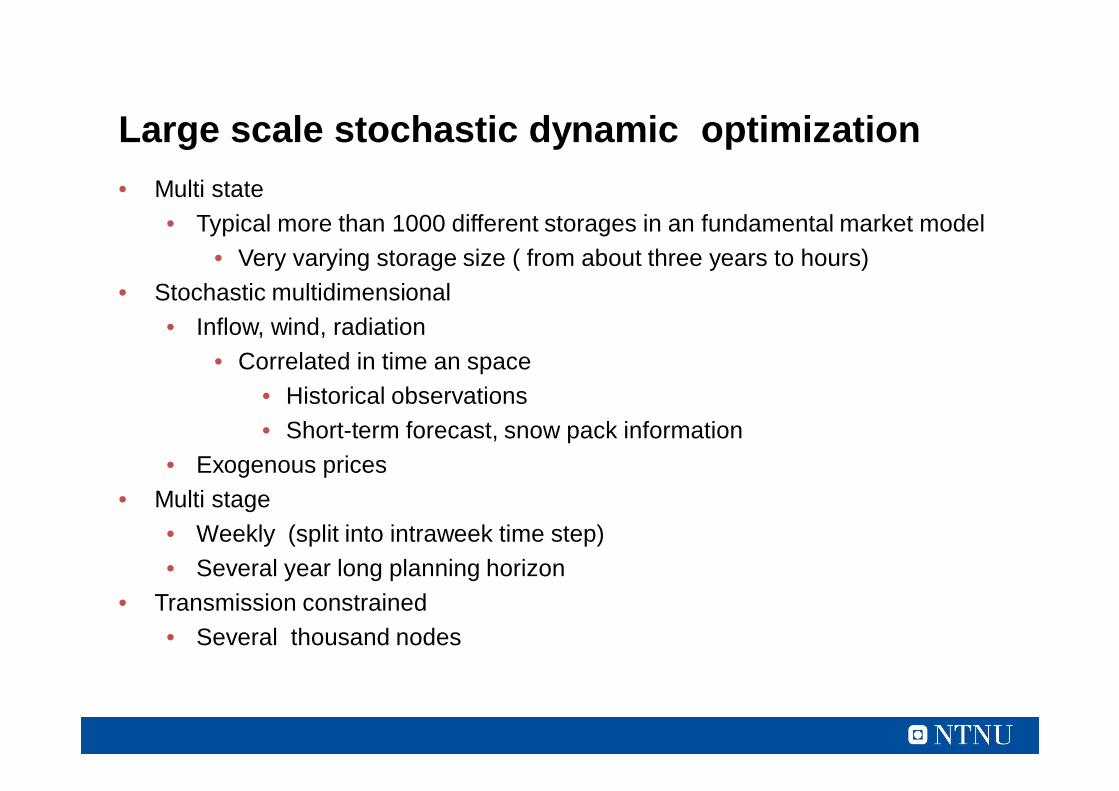
• Multi state• Typical more than 1000 different storages in an fundamental market model

• Very varying storage size ( from about three years to hours)• Stochastic multidimensional

• Inflow, wind, radiation• Correlated in time an space

• Historical observations• Short-term forecast, snow pack information

• Exogenous prices• Multi stage

• Weekly (split into intraweek time step)• Several year long planning horizon

• Transmission constrained• Several thousand nodes

Large scale stochastic dynamic optimization

Multi-area model ofNordic countries

V -S Ø

V -M I

H A L

T e l

Ø -L

G /L

H e l

T ro

N -M I

S -Ø -L

S -L

D Kø s t

E s tla n d

L a tv ia

L ita u e n

P o le nN e d

N o rdS v er ig e

F in

F in la n d

S ydS v er ig e

D Kv e s t

T y s k la n dE F I

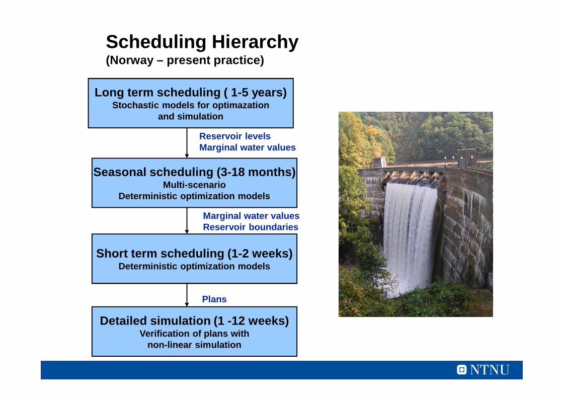
Scheduling Hierarchy(Norway – present practice)

Detailed simulation (1 -12 weeks)Verification of plans with

non-linear simulation

Long term scheduling ( 1-5 years)Stochastic models for optimazation

and simulation

Reservoir levelsMarginal water values

Seasonal scheduling (3-18 months)Multi-scenario

Deterministic optimization models

Marginal water valuesReservoir boundaries

Short term scheduling (1-2 weeks)Deterministic optimization models

Plans

9

Methods in use

• SDP (Long-term)– Aggregated– Stochastic

• SDDP (Long / Mid-term)– Detailed– Stochastic

• Scenario-based (Mid-term)– Deterministic

• Deterministic(Short-term)– LP– MIP– DP– Lagrange relaxation

Longer-term scheduling

Simulation of markets with storages and weather uncertainty

Storage possibilities Strategy by (SDP/SDDP) Markets and prices

Simulating markets (LP)Stochastic, inflowsolar, wind etc

Supply/demand data

Water value

Simulation

System operation

Storage utilization

Courtesy: Birger Mo, SINTEF

12

Marginal water values calculated for all pointsover the time horizon

20·1 + 28·5 + 30·9 + 35·20 + 40·9 + 60·5 + 70·1

4

2

070

60

1 2Tm7

Tm6

20 Tm128 Tm230 Tm335 Tm440 Tm5

92n-51

94

96

98100

Reservoir [%]

n2,0

n-1

1,51,00,80,5

0,0

0,0

48 49 50 51 52 uke

Iterate over the time horizon (n-52, n)

(1+ 5 + 9 + 20 + 9 + 5 + 1)VV4 = = 37,2 [øre/kWh]

13

Illustration of water values

00

0,8

1,0

Reservoir content [GWh]

week50 100 150 200

1,2

0,6

0,4

0,2

øre/kWh0

1020

3040

Application example – Integration of balancingmarkets

Detailed water course descriptionAbout 300 thermal power plantsTransmission corridors (NTC)

Fundamentalmodel

Denmark, Finland, Norway, SwedenGermany, Netherlands, Belgium

NorthernEurope

2010 – current state of the system2020 – a future state of the system

Systemscenarios

Hydrology (Inflow)TemperatureWind speed

Severalclimatic years

Coupling between models and planninglevels

16

Coupling between planning levels

• Different models at different planning levels complicates thecoupling and information flow

• The next level of analysis does not necessarily get input data ofsufficient precision

• Aggregation / disaggregation challenges

• Coupling principles:– Price coupling (individual / aggregated)– Volume coupling

Aggregation / disaggregation challenges

Shorter-term

Longer-term

Coupling principleIncremental water values

Shorter-term Longer-term

Reservoirlevel Flexible reservoir drawdown

with possibility to move waterbetween periods

Puts certain requirements on the methods usedin both periods

Short-term scheduling

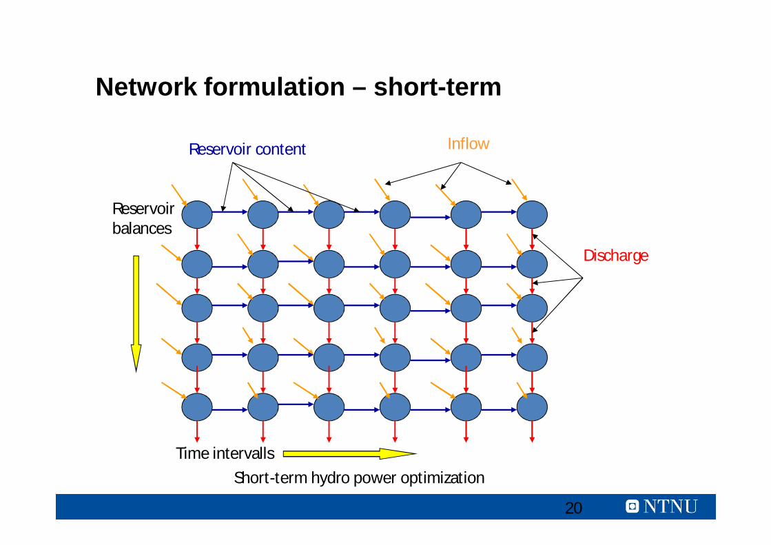
Short-term hydro power optimization

20

Network formulation – short-term

InflowReservoir content

Discharge

Time intervalls

Reservoirbalances

THANKS FOR YOUR ATTENTIONMore information: http://www.ntnu.edu/energy

22

Linear programming

• Linear models are fundamental for most the modeling andsimulation

• The experience shows that most of the physical problemscan be solved by using linear models as building blocks

• Non-linearities can be handles by:– Piece-wise linear segments– Iteration for successive refinement– Integer variable and to check combinations

• Algorithms are available to solve very large problems fast

Coupling principleVolume coupling

Shorter-term Longer-term

Reservoirlevel Specified reservoir

endpoint level

Less requirements to the methods used

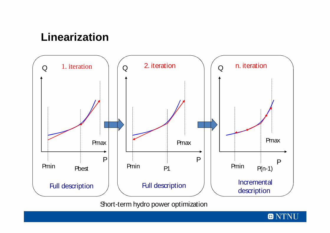
Linearization

P

Q

Pmin Pbest

Pmax

Q

Pmin P1

Pmax

Q

Pmin P(n-1)

Pmax

P P

1. iteration 2. iteration n. iteration

Full description Full description Incrementaldescription

Short-term hydro power optimization

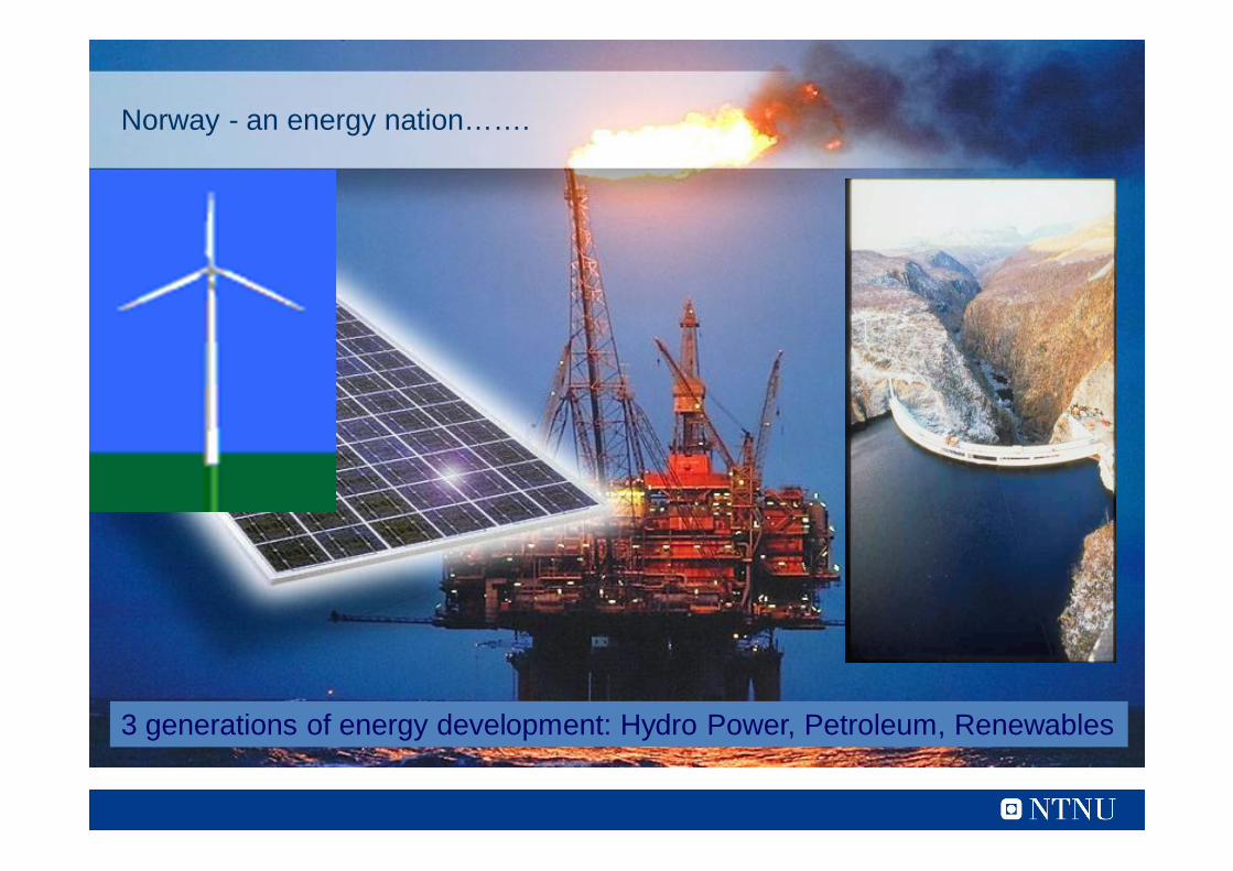
Norway - an energy nation…….

3 generations of energy development: Hydro Power, Petroleum, Renewables

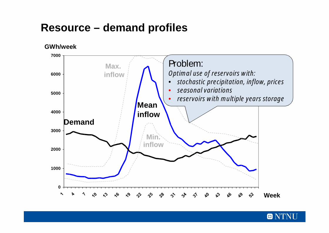
0

1000

2000

3000

4000

5000

6000

7000

Meaninflow

Demand

GWh/week

Week

Max.inflow

Min.inflow

Problem:Optimal use of reservoirs with:• stochastic precipitation, inflow, prices• seasonal variations• reservoirs with multiple years storage

Resource – demand profiles

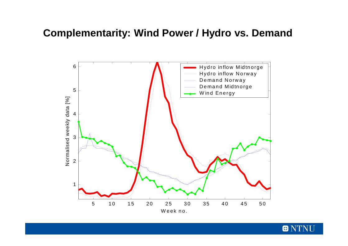
5 1 0 1 5 20 2 5 3 0 35 4 0 4 5 5 0

1

2

3

4

5

6

W e ek n o .

Nor

mal

ised

wee

kly

data

[%]

H yd ro in flow M id tn o rgeH yd ro in flow N o rw a yD e ma n d N o rw a yD e ma n d M id tn o rg eW in d En ergy

Complementarity: Wind Power / Hydro vs. Demand

28

Norwegian hydropower for balancing• The reservoirs are natural lakes

• Multi-year reservoirs• Largest lake stores 8 TWh• Total 84 TWh reservior capacity

• Balancing capacity estimates 2030• 29 GW installed at present• + 10 GW with larger tunnels and

generators• + 20 GW pumped storage• 30 GW total new capacity

• Within todays environmentallimits

• Requires more transmission capacityCourtesy: Birger Mo / CEDREN

Price difference between Norway and Germany– average week