Methodological Comparison of Cost-effectiveness of …bcap-energy.org/wp-content/.../ICF-Comparison-of-Cost-effectiveness... · Cost-effectiveness of IECC Residential Energy Codes

Methodological Comparison of

Cost-effectiveness of IECC Residential Energy Codes

Final Report

July 21, 2015

Submitted to:

Energy Efficient Codes Coalition

Prepared by:

ICF International 9300 Lee Highway Fairfax, VA 22031

2

blankpage

3

Table of Contents

Executive Summary .......................................................................................................................4

A. Introduction ..............................................................................................................................6

B. Pros and Cons of Each Cost-Effectiveness Methodology..................................................6 i. Life-cycle Cost .............................................................................................................................. 6 ii. Simple Payback ........................................................................................................................... 7 iii. Mortgage Cash Flow ................................................................................................................... 7

C. Key Elements of Sound Cost-Effectiveness Analysis ........................................................8

D. Scenario Analysis ....................................................................................................................9 i. Approach ....................................................................................................................................... 9 ii. Results ........................................................................................................................................ 11 iii. Comparison of Results and Key Findings.............................................................................. 14

Appendix A ................................................................................................................................... 15

Comparison of Cost-effectiveness Methodologies

4

Executive Summary ICF was asked to conduct an analysis of building energy codes, comparing life-cycle cost analysis (LCC) –

the predominant method used to evaluate the cost effectiveness of energy codes and other public

policies – with two other cost-effectiveness methods: simple payback and mortgage cash-flow. Since a

significant proposal before Congress would designate simple payback as the principal basis for energy

code cost-effectiveness, representing a departure from decades of policy analysis practice, it is

important to provide a robust comparison of simple payback to the LCC and mortgage cash-flow

methods.

Simple payback is typically used in the private sector to evaluate discrete, low-to-moderate-cost energy

retrofit projects in existing facilities. Mortgage cash-flow analysis is typically used to evaluate whole-

building transactions involving financing. LCC analysis can incorporate mortgage cash flow calculations

to the extent they account for the full useful life of energy efficiency measures. However, LCC is

fundamentally incompatible with simple payback analysis; many measures that may “fail” a simple

payback analysis can be cost-effective on an LCC basis.

A key issue in assessing cost-effectiveness of efficiency measures is capturing the value of savings over

the full useful life of the measure or building. Both the LCC and mortgage cash-flow methods

incorporate measures’ useful lives, which can vary from 5 years (e.g., lighting measures) to more than 30

years (e.g., insulation measures). By contrast, simple payback fails to recognize useful life; this is a

critical omission, and puts into question the appropriateness of simple payback for public policy analysis.

To help resolve these issues, this study provides a rigorous, consistent, quantified comparison of these

three methodologies. In addition to detailing quantified results, it discusses the pros and cons of each

method. The intent is to provide public policy analysts and policymakers additional clarity and insight

into these important issues.

Pre-eminence of Life-Cycle Cost Approach for Energy Codes and other Policies

Policymakers take the life-cycle perspective because buildings can last over 100 years, and only the long

view that accounts for all factors affecting the cost-effectiveness of efficiency improvements over the

full life of the building can ensure sound public policy decisions. In addition, the International Energy

Conservation Code (IECC) – which is the residential building code in 40 states, the District of Columbia,

and numerous local jurisdictions in the remaining states – specifically requires that energy efficiency be

considered “over the life of the building” (residential or commercial).

In conducting this life-cycle analysis, we employed widely-used and nationally-accepted National

Institute of Standards and Technology (NIST) methodologies, and used:

A nationally-accredited building simulation model to calculate energy savings,

Recognized federal and industry sources for cost estimates, and

Industry sources to quantify service life of efficiency measures.


5

Simple Payback

Simple payback is used principally by private investors to assess the time to recoup the cost of a single

energy efficiency retrofit. Its primary attribute is calculation simplicity, but because simple payback fails

to consider important financial elements – such as the full useful life of efficiency measures, the ways

most Americans actually buy homes, changes in fuel costs and energy bills, discount rates, and tax

implications – it is typically not used in public-policy cost-effectiveness assessments. In addition,

because the great majority of American home buyers use mortgage financing to buy their homes, simple

payback is not applicable to most home purchase transactions. Buyers who do pay cash are typically

either investors seeking to rent or flip the property, or wealthy individuals for whom affordability is not

an issue.

Mortgage Cash Flow

Building energy codes are developed and adopted to reduce homeowner and renter utility bills, which

account for the largest share of home occupancy costs after mortgage payment (or rent) and are the

least predictable cost of home ownership. To assess the cost-effectiveness of codes in the context of

home occupancy costs, it is most appropriate to apply a mortgage cash flow analysis method, which

projects the net occupancy costs associated with code-compliant homes. Tracking mortgage cash flow

paints a clear and realistic picture of building energy efficiency to a typical homeowner or occupant,

evaluating how quickly energy bill savings help the homeowner reach a break-even point with outlays

for efficiency improvements.

Key Findings

All of the methodologies were used to calculate the cost-effectiveness of two IECC stringency increases:

(1) the 2006 IECC to the 2012/2015a IECC, and (2) the 2009 IECC to the 2012/2015 IECC. Key findings

that emerge from this analysis include:

The 2012/2015 IECC is cost-effective on a lifecycle basis. Without exception, the LCC analysis

shows net present dollar savings of the 2012/2015 IECC in all U.S. climate zones, whether the

baseline code is the 2006 or 2009 IECC.

The 2012/2015 IECC delivers actual net savings to typical homeowners in the second year of

home ownership. The mortgage cash flow analysis shows positive cash flow in year 2, including

points later in the mortgage term when replacement costs occur.

Simple paybacks average less than 10 years. While paybacks exceed 10 years in some climate

zones, on a national average basis, the payback is under 10 years. This contrasts sharply with

other studies that show substantially longer paybacks, typically based on very high cost

estimates that do not jibe with the recognized, transparent sources used in this analysis.

a Because efficiency requirements of the 2015 IECC are virtually identical to those of the 2012 IECC, the energy savings attributed to the 2012 IECC in this analysis are also expected for homes built to the 2015 IECC. In its determination on the residential chapter of the 2015 IECC, the US Department of Energy found savings to be less than 1% greater than the 2012 IECC: “On June 11, 2015, DOE issued a determination that the 2015 IECC would achieve greater energy efficiency in buildings subject to the code. DOE estimates national savings in residential buildings of approximately: “0.73% energy cost savings “0.87% source energy savings “0.98% site energy savings”


6

A. Introduction The intent of this study is to compare and contrast the multiple cost-effective methodologies for

residential construction that have been discussed in the marketplace to date. These include: (1) Life-

cycle Cost, (2) Simple Payback, and (3) Mortgage Cash Flow.

This study examines the pros and cons of each of these methodologies, provides examples their

application to the same set of energy upgrades and costs, defines the three key common elements of

cost-effectiveness analysis, and compare the differing results from these differing methods.

Life-cycle cost analysis has been the primary methodology used in public policy analysis for many

decades, because policymakers take a long-term perspective that examines the full range of benefits

and costs. For example, U.S. Department of Energy cost-effectiveness methods typically apply

standardized life-cycle cost analysis methods developed by the National Institute of Standards and

Technology (NIST). Simple payback is a private market metric that examines the time to recoup first

costs of an investment. Mortgage cash flow analysis takes a homeowner perspective of the year-by-year

balance of costs and benefits in a typical home mortgage context.

B. Pros and Cons of Each Cost-Effectiveness Methodology

i. Life-cycle Cost

Life-cycle Cost analysis calculates the sum of all benefits and costs over a specified time period, typically

the service life of a building, technology, or project. In the context of this analysis, which examines the

cost-effectiveness of building code-mandated efficiency measures for a typical homeowner, it calculates

the net present value of the direct benefits and costs experienced by a typical homeowner, including

increased purchase price, energy cost savings, tax implications, varying fuel prices, and increased

property value. It brings back the stream of benefits and costs to a present value basis by applying a

discount rate.

Pros

Encompasses the full costs and benefits over the life of the building, as required in the IECC.

Applies standardized NIST life-cycle cost methods that are widely used across the federal

government.

Cons

Requires somewhat more complex analysis than simple payback, typically involving spreadsheet

calculations.


7

ii. Simple Payback

Simple payback is typically calculated the number of years required for energy cost savings to equal the

initial cost of efficient measures, without addressing service life of measures, changes in fuel prices,

discount rates, tax implications, resale value or other factors.

Pros

Simple to calculate.

Applied widely in private sector investment decision-making, where a single private entity is

seeking to assess the time to recoup the cost of a specific investment.

Cons

Does not address a policy perspective, which examines benefits and costs across the full lifetime

of the building/technology/project, beyond the perspective of the initial investor.

Does not capture the typical perspective of a homeowner, which involves mortgage financing.

Cash buyers are typically investors seeking to rent or flip the property, or are wealthy individuals

who are willing to pay full market value of the property.

Does not encompass the full service life of the building, as required in the IECC, or of the

individual efficiency measures in the building.

iii. Mortgage Cash Flow

Mortgage cash flow analysis calculates year-by-year annual net cash flow by comparing annualized cost

mortgage payment increases to annual energy savings, while also factoring in added down payment, tax

impacts and other factors. For example, if an efficient home’s added construction costs increase

mortgage payment by $350 per year and the annual energy savings are $400 per year, the annual cash

flow is $50. These calculations can also be incorporated in a life-cycle cost analysis.

Pros

Captures the most realistic perspective of the effect of energy codes on a typical homebuyer.

Provides a more accurate indicator than simple payback of the time to recoup increased home

construction costs.

Cons

Typically requires spreadsheet calculations beyond simple math.


8

C. Key Elements of Sound Cost-Effectiveness Analysis Three key inputs for cost-effectiveness calculations are required to achieve robust results:

1. Accurate estimation of incremental cost

Determining reasonable incremental costs for building components can be difficult, because

builders may not track incremental costs, or may be reluctant to divulge such cost details. Also,

market dynamics typically drive costs down for the most commonly used products or materials;

when energy codes shift standard specifications and practices, the new products and materials

typically come down in price as they become the predominant market choice. To address these

issues, ICF follows the common practice of policy analysts, consulting multiple robust sources to

converge on reasonable cost estimates: these typically include the NREL Residential Energy

Efficiency Measures Database, the PNNL Building Component Cost Community, and R.S. Means.

2. Accurate estimation of energy savings

It is important to use accredited, field-verified energy simulation tools that are provide location-

specific energy savings calculations, so that energy savings estimates are based on robust

analysis. Using default national values or basic percent savings values can create a skewed

picture or distort the policy implications of cost-effectiveness analyses.

3. Accurate estimation of component useful life

Accounting for the realistic service life of a piece of equipment or efficiency upgrade savings is

essential to assessing lifetime costs and benefits. For example an upgrade in shell insulation may

add a one-time $500 to home construction costs, but delivers energy savings for the entire life

of the home (30+ years). By contrast, high efficacy lighting may last approximately 5 years; while

its initial incremental cost may be $100, over the 30-year period of analysis it would be replaced

6 times, with lifetime costs of $600 exceeding that of the insulation upgrade.


9

D. Scenario Analysis

i. Approach

Each of the cost-effectiveness methodologies outlined in Section A above were applied to a typical new

single family home in locations across the country to compare the results using each methodology.

These cost-effectiveness methodologies are calculated to estimate the cost-effectiveness of two code

stringency increases: (1) the 2006 IECC to the 2012 IECC and (2) the 2009 IECC to the 2012 IECC.

ICF developed the following inputs for calculations using the three cost-effectiveness methodologies

outlined in Section A:

1. Annual energy savings (kWh, Therms)

2. Incremental construction costs ($)

3. Building component useful life (Years)

4. Energy prices ($)

5. Economic Assumptions (e.g. mortgage interest rate, inflation rate, discount rate)

The first input, annual energy savings, was calculated through more than 3,000 simulations using ICF’s

RESNET-accredited Beacon Residential software. These simulations encompassed 119 weather locations,

four foundation types, and two HVAC system types. Exhibit A4 of Appendix A displays the energy savings

results.

The housing characteristics analyzed are shown displayed in Exhibit 1, below. This home is of a typical

size for a new home in the United States, and aligns with the characteristics of the reference home

contained in the U.S. DOE’s Methodology for Evaluating Cost-Effectiveness of Residential Energy Code

Changes. A more detailed view that includes HVAC system types and foundation types is contained in

Exhibit A1 of Appendix A.

Exhibit 1: Housing Characteristicsb

Parameter Assumption

Conditioned Floor Area 2,400 ft2

Stories 2

Bedrooms 3

Locations 119 Weather Locations

across all IECC Climate Zones

The second set of inputs, the incremental costs for individual building component upgrades, was

determined from the NREL National Residential Energy Efficiency Measures Database and R.S. Means. A

full summary of incremental costs is contained in Exhibit A5 and A6 in Appendix A.

b U.S. DOE’s Methodology for Evaluating Cost-Effectiveness of Residential Energy Code Changes


10

The third set of inputs, the building component useful life, was sourced from the National Association of

Home Builders Study of Life Expectancy of Home Components report. These values are the median

length of time in which a building component operates/functions within a home before needing to be

replaced. A detailed summary of the useful life for each component is displayed in Exhibit A2 of

Appendix A.

The fourth required input, energy prices, were obtained from the U.S. Energy Information

Administration’s Annual Energy Outlook and are outlined in Exhibit A3 in Appendix A.

Lastly, the assumptions required to perform an economic analysis are contained in Exhibit A3 of

Appendix A. These values align with the assumptions contained in the U.S. DOE’s Methodology for

Evaluating Cost-Effectiveness of Residential Energy Code Changes.

Once all of these inputs were determined, they were input into ICF’s Economic Metrics Calculator, which

includes each of the three methodologies and is used to assess the cost-effectiveness of IECC code

changes and above-code programs including the ENERGY STAR Certified Homes program.


11

ii. Results

Life-cycle Cost

The life-cycle cost analysis for each of these code upgrades results in net benefits across all Climate

Zones, as shown in Exhibit 2, below. A negative life-cycle cost actually represents the positive net savings

to the homeowner over the life of the mortgage; for example, in Exhibit 2, Zone 4 net savings are $1543.

Exhibit 2 shows net savings for the 2012 IECC, compared to both the 2009 and 2009 versions, across all

climate zones. Net savings range from $502 to $9,232; taking Climate Zone 4 as a median mixed climate,

savings range from $1,543 to $2,975. The size of the net benefits increases when using the 2006 IECC as

the basis, because total energy savings are larger in that scenario.

Exhibit 2: Life-Cycle Cost Results

Climate Zone

Present Value Costs

Present Value Benefits

Life-Cycle Net Savings

2009 to 2012 IECC

1 $1,534 $2,036 $502

2 $1,660 $2,521 $861

3 $2,842 $4,412 $1,569

4 $2,674 $4,217 $1,543

5 $2,298 $3,572 $1,275

6 $1,808 $9,104 $7,295

7 $1,808 $9,627 $7,819

8 $1,808 $10,732 $8,923

2006 to 2012 IECC

1 $2,957 $5,575 $2,618

2 $2,686 $4,863 $2,177

3 $5,011 $6,850 $1,839

4 $3,642 $6,617 $2,975

5 $3,209 $5,396 $2,187

6 $3,072 $10,926 $7,853

7 $3,072 $11,332 $8,260

8 $3,072 $12,304 $9,232


12

Simple Payback

In applying the simple payback methodology, we used a threshold of 10 years or less as a proxy for cost-

effectiveness, as 10 years is often quoted as the maximum tenure of a first-time homebuyer, though in

some markets this may be as low as 3-5 years. As displayed in Exhibit 3, the analysis shows that in

several Climate Zones, the code upgrades do not meet either the 10-year or 3-5 year thresholds.

However, national average simple paybacks are under 10 years for both code upgrade scenarios; this

contrasts with sharply higher simple payback estimates developed by industry studies.

Exhibit 3: Simple Payback Results

Climate Zone

Incremental Upgrade Cost

Annual Energy Savings

Simple Payback (years)

2009 to 2012 IECC

1 $970 $78 12.5

2 $1,073 $98 11.0

3 $2,058 $172 12.0

4 $1,964 $165 11.9

5 $1,651 $139 11.8

6 $1,255 $377 3.3

7 $1,255 $400 3.1

8 $1,255 $447 2.8

2006 to 2012 IECC

1 $1,869 $219 8.5

2 $1,744 $191 9.1

3 $3,642 $262 13.9

4 $2,603 $261 10.0

5 $2,258 $212 10.7

6 $2,147 $448 4.8

7 $2,147 $465 4.6

8 $2,147 $506 4.2

Mortgage Cash Flow Analysis

Exhibit 4 displays the annual cash flow from the homeowner perspective over 30 years. This value varies

year to year as building components reach the end of their useful life and replacement costs are

incurred. For example, Exhibit 4 shows negative cash flow in years 10 and 20 as ductwork and other

measures incur new costs. See the useful life values noted in Exhibit A2 in Appendix A for specifics.

The key finding from this analysis is that the typical homeowner sees positive cash flow by Year 2 of

homeownership. Even when new costs are incurred later in the life-cycle, cash flow becomes positive

again within two years. This means that in the real world of homeownership, energy code upgrades pay

for themselves in less than two years.


13

For this analysis, ICF has aggregated these cash flow results into a single net present value number, and

included it in the life-cycle cost analysis. While mortgage cash flow analysis comes closest to the real-

world perspective of a typical homeowner, policymakers seeking guidance on building codes policy are

best served by established life-cycle cost analysis.

Exhibit 4: Cash Flow Results

2006 to 2012 IECC 2009 to 2012 IECC

1 2 3 4 5 6 7 8 1 2 3 4 5 6 7 8

0 -$106 -$112 -$371 -$192 -$181 $74 $92 $133 -$91 -$89 -$186 -$177 -$148 $159 $181 $228

1 $125 $103 $75 $129 $97 $346 $364 $406 $28 $43 $66 $64 $55 $321 $344 $393

2 $131 $109 $82 $137 $103 $359 $377 $421 $30 $46 $71 $69 $59 $333 $356 $406

3 $138 $114 $89 $144 $109 $373 $391 $437 $32 $49 $76 $73 $63 $344 $368 $420

4 $144 $120 $96 $152 $115 $387 $406 $452 $35 $51 $81 $78 $67 $356 $381 $434

5 $151 $126 $104 $160 $122 $401 $421 $469 $37 $54 $86 $83 $71 $368 $394 $449

6 $158 $132 $112 $168 $128 $416 $436 $486 $39 $57 $91 $88 $75 $381 $408 $464

7 $165 $138 $120 $176 $135 $431 $452 $503 $42 $61 $97 $93 $80 $394 $421 $479

8 $173 $145 $128 $185 $142 $447 $468 $521 $44 $64 $102 $99 $84 $407 $436 $495

9 $180 $151 $137 $194 $149 $463 $485 $539 $47 $67 $108 $104 $89 $421 $450 $511

10 -$42 -$72 -$84 -$26 -$73 $250 $273 $328 -$65 -$44 -$1 -$5 -$21 $321 $351 $414

11 $196 $165 $155 $213 $164 $496 $520 $577 $52 $74 $120 $116 $99 $450 $481 $546

12 $204 $172 $164 $222 $172 $514 $539 $597 $55 $78 $126 $122 $104 $465 $497 $564

13 $213 $180 $174 $232 $180 $532 $558 $618 $58 $81 $133 $128 $109 $481 $513 $582

14 $222 $187 $184 $243 $188 $551 $577 $639 $61 $85 $139 $134 $114 $497 $530 $601

15 $111 $76 $75 $134 $78 $451 $478 $542 -$55 -$30 $27 $22 $1 $394 $428 $501

16 $240 $203 $205 $264 $206 $590 $618 $684 $67 $93 $153 $148 $126 $530 $566 $641

17 $249 $211 $215 $275 $215 $610 $639 $707 $71 $97 $160 $155 $132 $547 $584 $662

18 $259 $220 $226 $287 $224 $631 $661 $731 $74 $102 $168 $162 $138 $565 $603 $683

19 $269 $229 $238 $299 $234 $653 $683 $755 $77 $106 $175 $169 $144 $584 $623 $705

20 -$634 -$364 -$308 -$17 -$66 $365 $396 $471 -$283 -$254 -$92 $42 -$11 $442 $482 $566

21 $290 $247 $261 $324 $254 $698 $730 $806 $85 $115 $191 $184 $157 $622 $664 $751

22 $301 $257 $274 $337 $264 $721 $754 $833 $88 $120 $199 $192 $163 $643 $685 $775

23 $313 $266 $287 $350 $275 $745 $779 $861 $92 $125 $208 $200 $170 $663 $707 $799

24 $324 $277 $300 $364 $286 $770 $805 $889 $96 $130 $217 $209 $177 $685 $730 $825

25 $336 $287 $313 $378 $297 $796 $832 $918 $100 $135 $226 $217 $185 $707 $753 $851

26 $349 $298 $327 $392 $309 $822 $860 $948 $104 $140 $235 $226 $192 $729 $777 $878

27 $361 $309 $341 $407 $321 $850 $888 $979 $109 $146 $244 $235 $200 $753 $802 $906

28 $374 $320 $356 $422 $333 $877 $917 $1,011 $113 $152 $254 $245 $208 $777 $827 $934

29 $388 $332 $370 $438 $345 $906 $947 $1,044 $118 $157 $264 $254 $216 $801 $853 $964

30 $402 $161 $178 $111 $5 $582 $624 $724 -$22 $19 $78 -$15 -$39 $563 $617 $730

Climate Zone

Year


14

iii. Comparison of Results and Key Findings

This section compares lifecycle cost and simple payback results using the methodology described above. Exhibit 5 summarizes this comparison; it shows divergent results, in that the life-cycle cost approach shows net cost savings across all Climate Zones, whereas the simple payback approach shows results that exceed 10 years in some Climate Zones. These differences can be explained by two factors:

Life-cycle cost analysis takes into account the total stream of savings over the lifetime of the building’s efficiency measures; simple payback does not.

Life-cycle cost analysis spreads the costs of energy code upgrades over a 30-year mortgage term, which is the typical homebuyer experience; simple payback assumes all costs are incurred in the first year. In a life-cycle cost analysis, only the incremental down payment is included in first-year costs.

Exhibit 5: Methodology Results Comparison

Climate Zone Simple Payback

(years) Life-Cycle Net

Savings

2009 IECC

1 12.5 $502

2 11.0 $861

3 12.0 $1,569

4 11.9 $1,543

5 11.8 $1,275

6 3.3 $7,295

7 3.1 $7,819

8 2.8 $8,923

2006 IECC

1 8.5 $2,618

2 9.1 $2,177

3 13.9 $1,839

4 10.0 $2,975

5 10.7 $2,187

6 4.8 $7,853

7 4.6 $8,260

8 4.2 $9,232

Key findings that emerge from this analysis include:

The 2012 IECC is cost-effective on a lifecycle basis. The LCC analysis shows net savings in all Climate Zones, whether the baseline code is the 2006 or 2009 IECC.

The 2012 IECC delivers net savings to typical homeowners in the second year of home ownership. The mortgage cash flow analysis shows positive cash flow in year 2, even later in the mortgage term when replacement costs occur.

Simple paybacks average less than 10 years. While paybacks exceed 10 years in some climate zones, on a national average basis the payback is under 10 years. This contrasts sharply with other studies that show substantially higher paybacks, typically based on very high cost estimates that do not jibe with the recognized, transparent sources used in this analysis.


15

Appendix A

Exhibit A1: Expanded Housing Configurationc

Parameter Assumption

Housing Type Single Family Detached

Conditioned Floor Area 2,400 ft2

Ceiling Height 8.5 ft

Perimeter 30 x 40 ft

Bedrooms 3

Window to Floor Area 15%

Window Destruction Even

Locations 119 Weather Locations

Heating System Types Natural Gas Furnace

Heat Pump

Cooling System Types Central AC

Heat Pump

Domestic Hot Water System Types

Gas Tank Water Heater

Electric Tank Water Heater

Foundation Types

Slab-on-grade

Unconditioned basement

Conditioned basement

Vented crawlspace

Exhibit A2: Building Component Useful life

Component Assumptions Source

Insulation / Shell 30+ years NAHBd

Framing Members 30+ years NAHB

Windows 20 years NAHB

Ventilation Systems 15 years NAHB

Ductwork (sealing) 10 years NAHB

High Efficacy Lighting 5.4 years ENERGY STARe

c U.S. DOE’s Methodology for Evaluating Cost-Effectiveness of Residential Energy Code Changes d NAHB Life Expectancy of Home Systems and Components e ENERGY STAR lighting product calculator


16

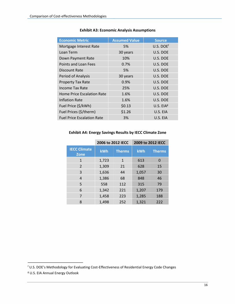
Exhibit A3: Economic Analysis Assumptions

Economic Metric Assumed Value Source

Mortgage Interest Rate 5% U.S. DOEf

Loan Term 30 years U.S. DOE

Down Payment Rate 10% U.S. DOE

Points and Loan Fees 0.7% U.S. DOE

Discount Rate 5% U.S. DOE

Period of Analysis 30 years U.S. DOE

Property Tax Rate 0.9% U.S. DOE

Income Tax Rate 25% U.S. DOE

Home Price Escalation Rate 1.6% U.S. DOE

Inflation Rate 1.6% U.S. DOE

Fuel Price ($/kWh) $0.13 U.S. EIAg

Fuel Prices ($/therm) $1.26 U.S. EIA

Fuel Price Escalation Rate 3% U.S. EIA

Exhibit A4: Energy Savings Results by IECC Climate Zone

2006 to 2012 IECC 2009 to 2012 IECC

IECC Climate Zone

kWh Therms kWh Therms

1 1,723 1 613 0

2 1,309 21 628 15

3 1,636 44 1,057 30

4 1,386 68 848 46

5 558 112 315 79

6 1,342 221 1,207 179

7 1,458 223 1,285 188

8 1,498 252 1,321 222

f U.S. DOE’s Methodology for Evaluating Cost-Effectiveness of Residential Energy Code Changes g U.S. EIA Annual Energy Outlook


17

Exhibit A5: Incremental Cost Assumptions – 2006 IECC to 2012 IECC

IECC Climate Zone

Building Component 1 2 3 4 5 6 7 8

Ceiling Insulation $0 $102 $102 $111 $111 $0 $0 $0

Wall Framing $0 $0 $375 $375 $0 $0 $0 $0

AG Wall Insulation $0 $0 $242 $242 $0 $0 $0 $0

Window $469 $242 $210 $43 $30 $30 $30 $30

Infiltration $960 $960 $1,392 $1,392 $1,392 $1,392 $1,392 $1,392

Vent $94 $94 $94 $94 $94 $94 $94 $94

BG Wall Insulation $0 $0 $881 $0 $286 $286 $286 $286

Ducts $196 $196 $196 $196 $196 $196 $196 $196

HVAC Insulation $50 $50 $50 $50 $50 $50 $50 $50

Lighting $100 $100 $100 $100 $100 $100 $100 $100

Total $1,869 $1,744 $3,642 $2,603 $2,258 $2,147 $2,147 $2,147

Exhibit A6: Incremental Cost Assumptions – 2009 IECC to 2012 IECC

IECC Climate Zone

Building Component 1 2 3 4 5 6 7 8

Ceiling Insulation $0 $102 $102 $111 $111 $0 $0 $0

Wall Framing $0 $0 $375 $375 $0 $0 $0 $0

AG Wall Insulation $0 $0 $242 $242 $0 $0 $0 $0

Window $167 $167 $102 $0 $19 $19 $19 $19

Infiltration $528 $528 $960 $960 $960 $960 $960 $960

Vent $94 $94 $94 $94 $94 $94 $94 $94

BG Wall Insulation $0 $0 $0 $0 $286 $0 $0 $0

Ducts $98 $98 $98 $98 $98 $98 $98 $98

HVAC Insulation $50 $50 $50 $50 $50 $50 $50 $50

Lighting $33 $33 $33 $33 $33 $33 $33 $33

Total $970 $1,073 $2,058 $1,964 $1,651 $1,255 $1,255 $1,255

Documents

Methodological Comparison of Cost-effectiveness of …bcap-energy.org/wp-content/.../ICF-Comparison-of-Cost-effectiveness... · Cost-effectiveness of IECC Residential Energy Codes