Mergers when Firms Compete by Choosing both Price and Promotion

Mergers when Firms Compete by Choosing both Price and Promotion

Steven Tenn1 Federal Trade Commission, Washington, DC 20580

Luke Froeb2 & Steven Tschantz3

Vanderbilt University, Nashville, TN 37203

April 11, 2007

Abstract

Enforcement agencies have a relatively good understanding of how to measure the loss of price

competition caused by merger. However, when firms compete in multiple dimensions, merger effects

are not well understood. In this paper, we study mergers in industries where firms compete by setting

both price and promotion, and ask what happens if we mistakenly assume that price is the only

dimension of competition. To answer the question, we build a structural model of the super-premium

ice cream industry, where a 2003 merger between Häagen-Dazs and Dreyer’s was challenged by the

Federal Trade Commission. A structural merger model that ignores promotional competition under-

predicts the price effects of a merger in this industry (5% instead of 12%). About three-fourths of the

difference can be attributed to estimation bias (estimated demand is too elastic), with the remainder due

to extrapolation bias from assuming post-merger promotional activity stays constant (instead it declines

by 31%).

DISCLAIMER: The views expressed in this paper do not purport to represent the views of the U.S. Federal Trade Commission, nor any of its Commissioners. We wish to acknowledge useful discussions with Hajime Hadeishi, David Schmidt, Timothy Muris, David Scheffman, Robert McMillan, Craig Peters, Henry Schneider, Shawn Ulrick, Matthew Weinberg, David Weiskopf, Gregory Werden, and participants at Cornell, Duke, and FTC workshops.

1 [email protected]

2Corresponding author: [email protected]

3 [email protected]

- 1 -

1. Introduction

Antitrust laws prohibit mergers that substantially lessen competition, and most often this means

mergers that raise price. Enforcement agencies have a relatively good understanding of price

competition, and how to measure the loss of price competition caused by merger. However, merger

effects are not well understood when firms compete in multiple dimensions, such as price, product,

place, and promotion.4 In this paper, we study mergers in industries where firms compete by setting

both price and promotion, and ask what happens if we mistakenly assume that price is the only

dimension of competition.

To answer the question, we build a structural merger model where firms compete using both

price and promotion. We find two sources of potential bias from ignoring promotional competition.

The first is what we call “estimation bias,” a type of omitted variables bias. If promotion is correlated

with price, then observed price changes will proxy for unobserved (or ignored) changes in promotional

activity. As a consequence, price elasticity estimates will be biased. Bias in estimated own-price

elasticities affects the post-merger price prediction because a merged firm facing a more elastic demand

would not raise price as high as a merged firm facing a less elastic demand (all else equal).

The second source of potential bias is what we call “extrapolation bias.” Following a merger, we

would expect the merged firm to internalize both price and promotional competition among its

commonly owned products. In price-only merger models, promotional activity is implicitly held

constant at pre-merger levels when the post-merger equilibrium is calculated. This leads to

extrapolation bias when optimal price depends on the level of promotional activity.

Interestingly, both types of bias depend on whether promotional activity makes demand more or

less elastic. If promotion makes demand more elastic, as we find, then optimal price will decline as

promotion increases. In this case, if promotional activity is ignored when estimating demand then price

decreases will proxy for the effects of increased promotion and make demand appear more elastic than it

4 These are the “4 P’s” of marketing (McCarthy, 1981).

- 2 -

actually is. Likewise, if promotional activity is ignored when computing the post-merger equilibrium, it

is implicitly held fixed at pre-merger levels, leading to more elastic demand than if promotional activity

were allowed to decline post-merger. Since a higher elasticity of demand leads to smaller merger

effects, both sources of bias attenuate the predicted post-merger price increase when promotions make

demand more elastic.

We find evidence of both estimation and extrapolation bias in the US super-premium ice cream

industry, where the Federal Trade Commission (FTC) challenged a 2003 merger between Häagen-Dazs

and Dreyer’s.5 We build a structural oligopoly model of this industry in which each firm competes by

setting both price and promotional activity, and use this model to simulate the effects of merger. The

results are then compared to counterpart estimates from a price-only model. The structural model which

ignores promotion under-predicts the price effects of a merger in this industry (5% instead of 12%).

About three-fourths of the difference can be attributed to estimation bias (estimated demand is too

elastic), with the remainder due to extrapolation bias from assuming post-merger promotional activity

stays constant (instead it declines by 31%).

In what follows, we first review the literature on merger modeling and then propose a framework

that allows us to characterize conditions under which estimation and extrapolation bias is likely to

appear. Finally, we present an empirical application in which the bias is significant.

2. How reliable are structural merger models?

To determine whether a proposed merger is anticompetitive, enforcement agencies must be able

to predict its effects. Merger predictions from structural oligopoly models are made in two distinct

steps. First, a model of firm and consumer behavior is estimated from observed pre-merger data. Then,

the estimated model parameters are used to forecast post-merger prices as the merged firm internalizes

competition among commonly owned products. The difference between observed pre-merger prices and

5 Super-premium ice cream is distinct from other types of ice cream; it has more butterfat, less air, and a

significantly higher price. The Federal Trade Commission found that super-premium ice cream is sufficiently differentiated that it comprises a separate product market (http://www.ftc.gov/os/2003/06/dreyercomplaint.htm).

- 3 -

predicted post-merger prices is an estimate of the merger effect. The popularity of the methodology and

its use to inform enforcement decisions has raised questions about its reliability (Werden et al., 2004;

Hosken et al., 2005).

Tests of model reliability have taken three forms. The first is to test over-identifying model

restrictions. For example, Werden (2000) and Pinske and Slade (2004) compare pre-merger price-cost

margins to demand elasticities in the Chicago bread industry and the UK brewing industry, respectively.

They find that the familiar margin-elasticity relationship of Bertrand models holds in the pre-merger

data. However, Kim and Knittel (2006) find that the margin-elasticity relationship does not hold in the

California electricity market.

A second test of model reliability is to determine how well structural models can predict actual

events. Nevo (2000) finds that predicted price changes are close to actual price changes for two mergers

in the ready-to-eat cereal industry. However, Peters (2006) finds that simulation methods “do not

generally provide an accurate forecast” of post-merger prices for five airline mergers. Using

information from the post-merger period, he finds that the merger prediction error is caused by

unobserved cost changes or firm behavioral changes. Hadeishi and Schmidt (2004) find that a structural

model could not predict the effects of a merger between two complements (peanut butter and jelly)

because demand shifted post-merger. Lastly, Weinberg (2005) finds that a structural model under-

predicts the price effects of a merger among producers of motor oil and over-predicts the price effects of

a merger among breakfast syrup producers.

Testing whether models can accurately predict real events is difficult because it requires

estimating both a structural model as well as the merger effect. The latter requires controls for

confounding factors that could cause post-merger prices to change. Typically, a difference-in-difference

estimator is used to compare prices of the merging firms to a set of control prices. The difficulties of

this approach were the subject of recent FTC hearings (FTC, 2005) on whether the oil mergers in the

late 1990’s increased the price of gasoline. Panelists raised questions about the choice of control group,

the choice of variables, the maintained assumptions behind the difference-in-difference estimator, and

the selection bias that follows from antitrust enforcement as agencies challenge only mergers that are

- 4 -

thought to be anticompetitive. The panel concluded that more study is needed to reliably answer the

question that motivated the hearings.

The third approach to testing model reliability is to determine the sensitivity of post-merger

predictions to the behavioral assumptions on which the models are built. Bertrand models of

competition, for example, assume that consumers choose products based on the price differences

between them, and that firms compete solely on the basis of price (e.g., Hausman et al., 1994; Werden

and Froeb, 1994). This is a simplification of the way consumers and firms actually behave, but models

necessarily abstract away from reality. Finding that a model is unrealistic is neither surprising nor

interesting. Rather, we want to know whether a model is unrealistic in ways that make its predictions

misleading. There are a number of studies that try to address this issue.

Gandhi et al. (forthcoming) find that if firms can change their “locations” in product space, in

addition to price, the merged firm will move its products apart to avoid cannibalizing sales. Since this

reduces the incentive to raise price, ignoring such repositioning overstates the effects of a merger.

Similarly, Froeb et al. (2003) find that capacity constraints on the non-merging firms amplify merger

effects, just as capacity constraints on the merging firms attenuate them. Since the latter effect is

typically bigger than the former, ignoring the effects of capacity constraints likely overstates the effects

of a merger. Crooke et al. (1999) and Froeb et al. (2005) find that demand functional form determines,

to an extent, the predicted merger effect. They recommend either sensitivity analysis, or computing

what they call “compensating marginal cost reductions,” the reductions in marginal cost necessary to

offset the merger effect. These depend only on elasticities, and not on demand functional form

(Werden, 1996). Finally, several authors have found that the downstream price effects of upstream

manufacturing mergers are determined, in part, by the vertical relationship between manufacturers and

retailers. Depending on the types of agreements between manufacturers and retailers, the retail sector

can attenuate, amplify, or completely hide the effects of upstream manufacturing mergers (Froeb et al.,

2007; O’Brien and Shaffer, 2005).

This paper follows this third strand of research by asking whether ignoring competition based on

promotional expenditures biases the predictions of structural merger models.

- 5 -

3. When does promotion matter for merger analysis?

In this section, we specify a simple canonical model of price and promotional competition as a

static non-cooperative game that is typical of the kinds of structural models used to predict merger

effects. We discover a correspondence between firm behavior in a price-plus-promotion model and firm

behavior in a price-only model that allows us to characterize the estimation bias that comes from

ignoring promotion. We also find that, under general conditions, firms have an incentive to change

promotion and price in the post-merger equilibrium. Extrapolation bias arises in price-only models that

mistakenly hold promotion fixed at pre-merger levels.

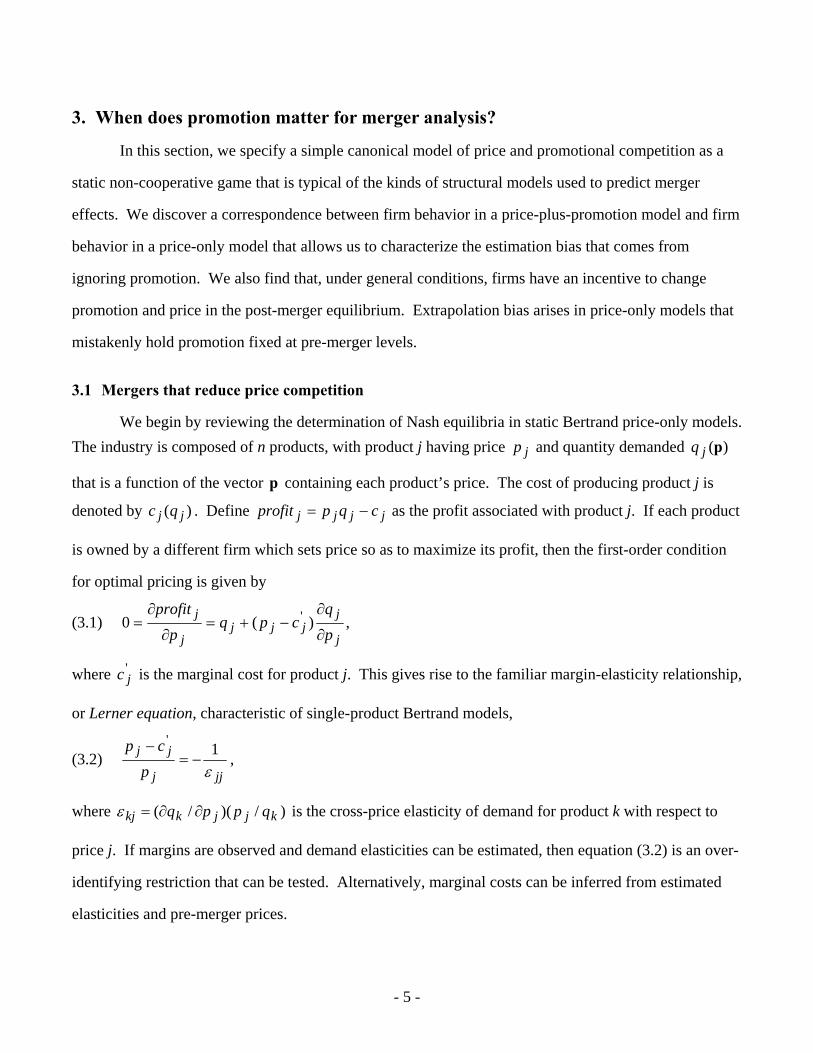
3.1 Mergers that reduce price competition

We begin by reviewing the determination of Nash equilibria in static Bertrand price-only models. The industry is composed of n products, with product j having price jp and quantity demanded )(pjq

that is a function of the vector p containing each product’s price. The cost of producing product j is

denoted by )( jj qc . Define jjjj cqpprofit −= as the profit associated with product j. If each product

is owned by a different firm which sets price so as to maximize its profit, then the first-order condition

for optimal pricing is given by

(3.1) j

jjjj

j

j

pq

cpqp

profit∂

∂−+=

∂

∂= )(0 ' ,

where 'jc is the marginal cost for product j. This gives rise to the familiar margin-elasticity relationship,

or Lerner equation, characteristic of single-product Bertrand models,

(3.2) jjj

jj

pcp

ε1'

−=−

,

where )/)(/( kjjkkj qppq ∂∂=ε is the cross-price elasticity of demand for product k with respect to

price j. If margins are observed and demand elasticities can be estimated, then equation (3.2) is an over-

identifying restriction that can be tested. Alternatively, marginal costs can be inferred from estimated

elasticities and pre-merger prices.

- 6 -

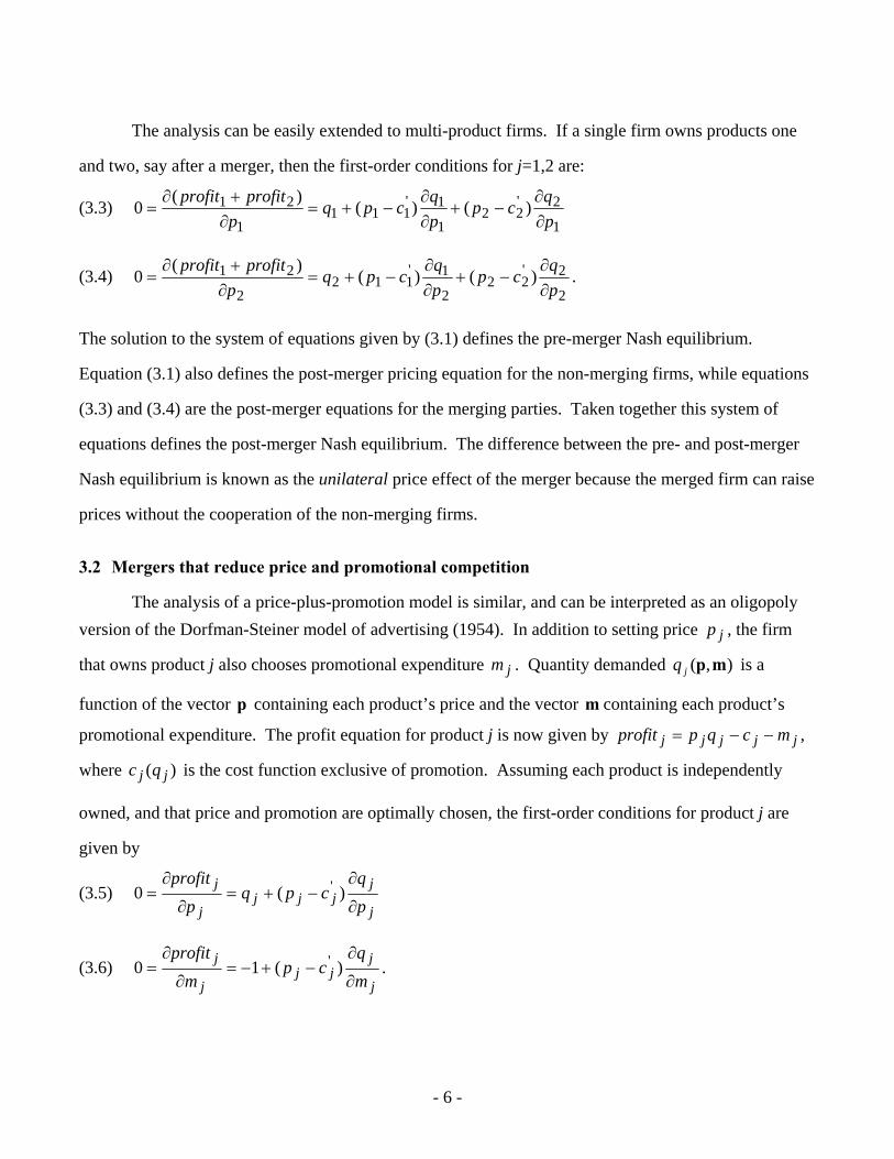
The analysis can be easily extended to multi-product firms. If a single firm owns products one

and two, say after a merger, then the first-order conditions for j=1,2 are:

(3.3) 1

2'22

1

1'111

1

21 )()()(0pqcp

pqcpq

pprofitprofit

∂∂

−+∂∂

−+=∂+∂

=

(3.4) 2

2'22

2

1'112

2

21 )()()(

0pq

cppq

cpqp

profitprofit∂∂

−+∂∂

−+=∂+∂

= .

The solution to the system of equations given by (3.1) defines the pre-merger Nash equilibrium.

Equation (3.1) also defines the post-merger pricing equation for the non-merging firms, while equations

(3.3) and (3.4) are the post-merger equations for the merging parties. Taken together this system of

equations defines the post-merger Nash equilibrium. The difference between the pre- and post-merger

Nash equilibrium is known as the unilateral price effect of the merger because the merged firm can raise

prices without the cooperation of the non-merging firms.

3.2 Mergers that reduce price and promotional competition

The analysis of a price-plus-promotion model is similar, and can be interpreted as an oligopoly version of the Dorfman-Steiner model of advertising (1954). In addition to setting price jp , the firm

that owns product j also chooses promotional expenditure jm . Quantity demanded ),( mpjq is a

function of the vector p containing each product’s price and the vector m containing each product’s

promotional expenditure. The profit equation for product j is now given by jjjjj mcqpprofit −−= ,

where )( jj qc is the cost function exclusive of promotion. Assuming each product is independently

owned, and that price and promotion are optimally chosen, the first-order conditions for product j are

given by

(3.5) j

jjjj

j

j

pq

cpqp

profit∂

∂−+=

∂

∂= )(0 '

(3.6) j

jjj

j

j

mq

cpm

profit∂

∂−+−=

∂

∂= )(10 ' .

- 7 -

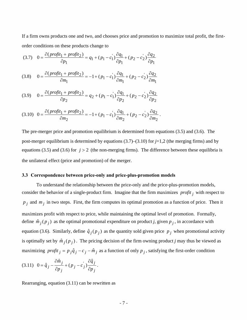
If a firm owns products one and two, and chooses price and promotion to maximize total profit, the first-

order conditions on these products change to

(3.7) 1

2'22

1

1'111

1

21 )()()(

0pq

cppq

cpqp

profitprofit∂∂

−+∂∂

−+=∂+∂

=

(3.8) 1

2'22

1

1'11

1

21 )()(1)(

0mq

cpmq

cpm

profitprofit∂∂

−+∂∂

−+−=∂+∂

=

(3.9) 2

2'22

2

1'112

2

21 )()()(

0pq

cppq

cpqp

profitprofit∂∂

−+∂∂

−+=∂+∂

=

(3.10) 2

2'22

2

1'11

2

21 )()(1)(

0mq

cpmq

cpm

profitprofit∂∂

−+∂∂

−+−=∂+∂

= .

The pre-merger price and promotion equilibrium is determined from equations (3.5) and (3.6). The

post-merger equilibrium is determined by equations (3.7)–(3.10) for j=1,2 (the merging firms) and by

equations (3.5) and (3.6) for 2>j (the non-merging firms). The difference between these equilibria is

the unilateral effect (price and promotion) of the merger.

3.3 Correspondence between price-only and price-plus-promotion models

To understand the relationship between the price-only and the price-plus-promotion models, consider the behavior of a single-product firm. Imagine that the firm maximizes jprofit with respect to

jp and jm in two steps. First, the firm computes its optimal promotion as a function of price. Then it

maximizes profit with respect to price, while maintaining the optimal level of promotion. Formally, define )(ˆ jj pm as the optimal promotional expenditure on product j, given jp , in accordance with

equation (3.6). Similarly, define )(ˆ jj pq as the quantity sold given price jp when promotional activity

is optimally set by )(ˆ jj pm . The pricing decision of the firm owning product j may thus be viewed as

maximizing jjjjj mcqpprofit ˆˆ −−= as a function of only jp , satisfying the first-order condition

(3.11) j

jjj

j

jj p

qcp

pm

q∂

∂−+

∂

∂−=

ˆ)(

ˆˆ0 ' .

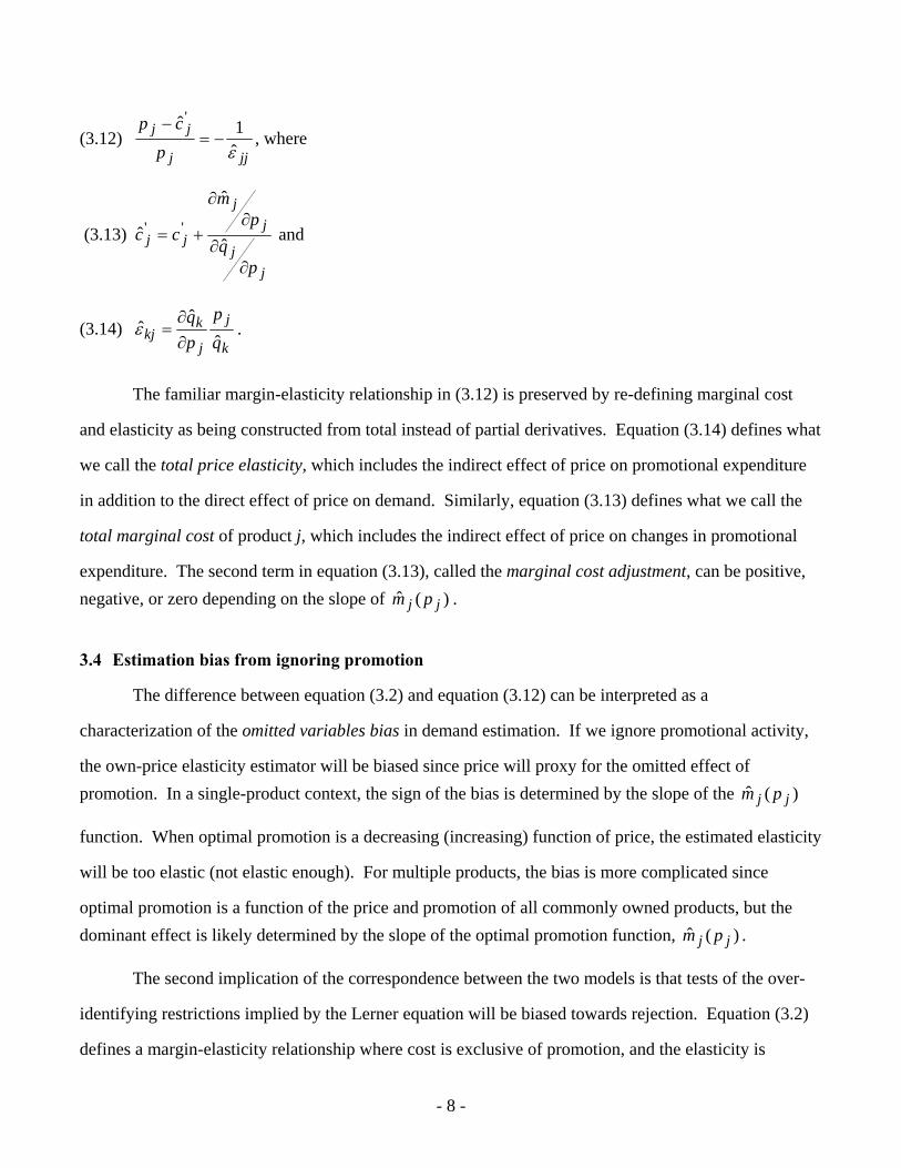
Rearranging, equation (3.11) can be rewritten as

- 8 -

(3.12) jjj

jj

pcp

ε̂1ˆ'

−=−

, where

(3.13)

jj

jj

jj

pq

pm

cc

∂∂

∂∂

+= ˆ

ˆ

ˆ '' and

(3.14) k

j

j

kkj q

ppq

ˆˆˆ

∂∂

=ε .

The familiar margin-elasticity relationship in (3.12) is preserved by re-defining marginal cost

and elasticity as being constructed from total instead of partial derivatives. Equation (3.14) defines what

we call the total price elasticity, which includes the indirect effect of price on promotional expenditure

in addition to the direct effect of price on demand. Similarly, equation (3.13) defines what we call the

total marginal cost of product j, which includes the indirect effect of price on changes in promotional

expenditure. The second term in equation (3.13), called the marginal cost adjustment, can be positive, negative, or zero depending on the slope of )(ˆ jj pm .

3.4 Estimation bias from ignoring promotion

The difference between equation (3.2) and equation (3.12) can be interpreted as a

characterization of the omitted variables bias in demand estimation. If we ignore promotional activity,

the own-price elasticity estimator will be biased since price will proxy for the omitted effect of promotion. In a single-product context, the sign of the bias is determined by the slope of the )(ˆ jj pm

function. When optimal promotion is a decreasing (increasing) function of price, the estimated elasticity

will be too elastic (not elastic enough). For multiple products, the bias is more complicated since

optimal promotion is a function of the price and promotion of all commonly owned products, but the dominant effect is likely determined by the slope of the optimal promotion function, )(ˆ jj pm .

The second implication of the correspondence between the two models is that tests of the over-

identifying restrictions implied by the Lerner equation will be biased towards rejection. Equation (3.2)

defines a margin-elasticity relationship where cost is exclusive of promotion, and the elasticity is

- 9 -

computed using partial derivatives. Alternatively, equation (3.12) defines a margin-elasticity

relationship where cost includes the indirect effect of price on changes in promotional expenditure, and

the elasticity is computed using total derivatives. While both are equally valid in the price-plus-

promotion model, the margin-elasticity relationship will not hold if one attempts to match the price

elasticity from equation (3.12) to the price-cost margin defined in equation (3.2). As such, tests of the

Lerner equation will be biased towards rejection in models where promotional competition is ignored, except in the case where optimal promotion is independent of price (i.e., 0/ˆ =∂∂ jj pm ).

3.5 Extrapolation bias from ignoring promotion

Extrapolation bias arises when promotional activity is mistakenly held fixed at pre-merger levels

when solving for the post-merger equilibrium. In this section, we develop a merger characterization that

includes the effects of promotion and show that, in general, promotional expenditure changes from the

pre- to the post-merger equilibrium. These changes affect post-merger pricing. The merger

characterization is built around “compensating marginal cost reductions” and pass-through rates (i.e., the

extent to which changes in marginal cost are passed through to price).

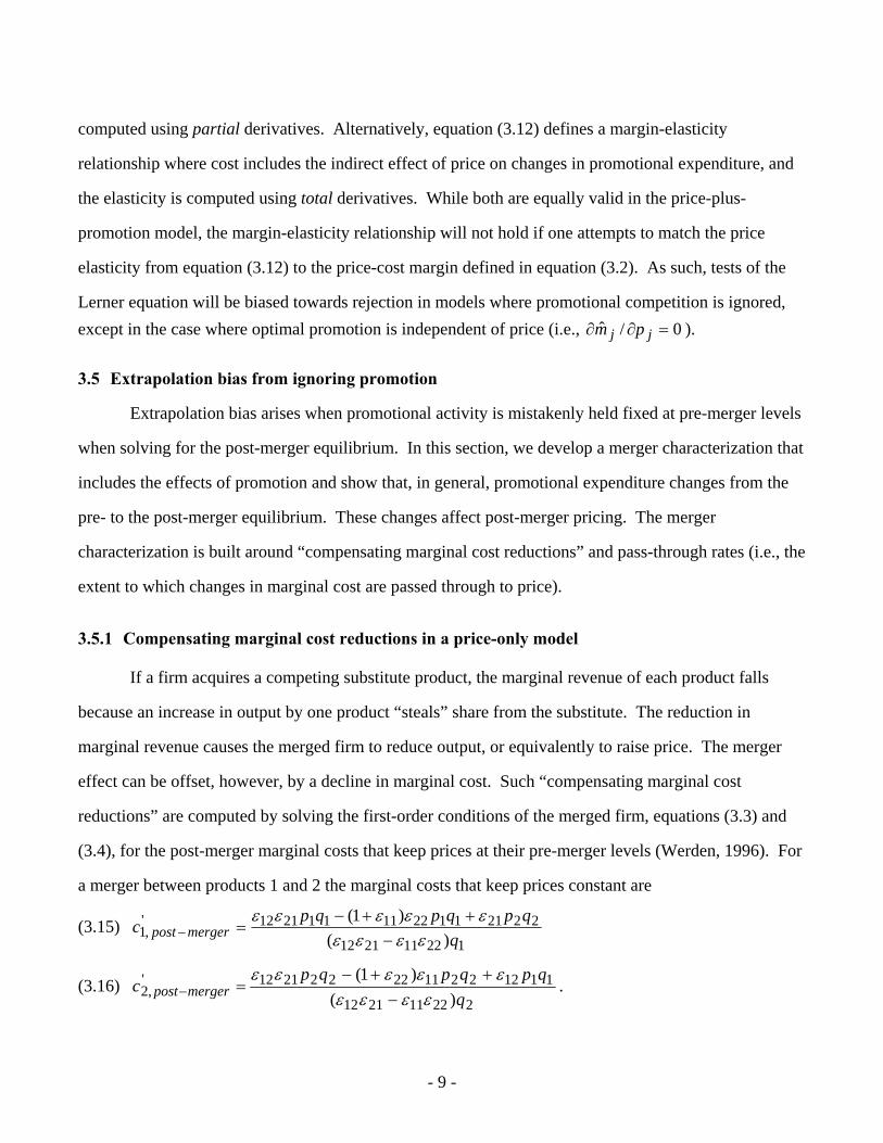
3.5.1 Compensating marginal cost reductions in a price-only model

If a firm acquires a competing substitute product, the marginal revenue of each product falls

because an increase in output by one product “steals” share from the substitute. The reduction in

marginal revenue causes the merged firm to reduce output, or equivalently to raise price. The merger

effect can be offset, however, by a decline in marginal cost. Such “compensating marginal cost

reductions” are computed by solving the first-order conditions of the merged firm, equations (3.3) and

(3.4), for the post-merger marginal costs that keep prices at their pre-merger levels (Werden, 1996). For

a merger between products 1 and 2 the marginal costs that keep prices constant are

(3.15) 122112112

2221112211112112',1 )(

)1(q

qpqpqpc mergerpost εεεε

εεεεε−

++−=−

(3.16) 222112112

1112221122222112',2 )(

)1(q

qpqpqpc mergerpost εεεε

εεεεε−

++−=− .

- 10 -

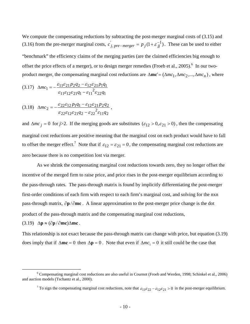
We compute the compensating reductions by subtracting the post-merger marginal costs of (3.15) and (3.16) from the pre-merger marginal costs, )1( 1'

,−

− += jjjmergerprej pc ε . These can be used to either

“benchmark” the efficiency claims of the merging parties (are the claimed efficiencies big enough to

offset the price effects of a merger), or to design merger remedies (Froeb et al., 2005).6 In our two-

product merger, the compensating marginal cost reductions are ),...,,(' 21 nmcmcmc ∆∆∆=∆mc , where

(3.17) 122

2111211211

1121122221111

qq

qpqpmcεεεεε

εεεε

−

−−=∆

(3.18) 211

2222211222

2221121112222

qq

qpqpmcεεεεε

εεεε

−

−−=∆ ,

and 0=∆ jmc for j>2. If the merging goods are substitutes )0,0( 2112 >> εε , then the compensating

marginal cost reductions are positive meaning that the marginal cost on each product would have to fall

to offset the merger effect.7 Note that if 02112 == εε , the compensating marginal cost reductions are

zero because there is no competition lost via merger.

As we shrink the compensating marginal cost reductions towards zero, they no longer offset the

incentive of the merged firm to raise price, and price rises in the post-merger equilibrium according to

the pass-through rates. The pass-through matrix is found by implicitly differentiating the post-merger

first-order conditions of each firm with respect to each firm’s marginal cost, and solving for the nxn

pass-through matrix, mcp ∂∂ / . A linear approximation to the post-merger price change is the dot

product of the pass-through matrix and the compensating marginal cost reductions,

(3.19) mcmcpp ∆∂∂≈∆ )/( .

This relationship is not exact because the pass-through matrix can change with price, but equation (3.19)

does imply that if 0=∆mc then 0=∆p . Note that even if 01 =∆mc it still could be the case that

6 Compensating marginal cost reductions are also useful in Cournot (Froeb and Werden, 1998; Schinkel et al., 2006)

and auction models (Tschantz et al., 2000).

7 To sign the compensating marginal cost reductions, note that 021122211 >− εεεε in the post-merger equilibrium.

- 11 -

01 >∆p because the off-diagonal elements of the pass-through matrix are non-zero, i.e., 2mc∆ can

affect 1p∆ .

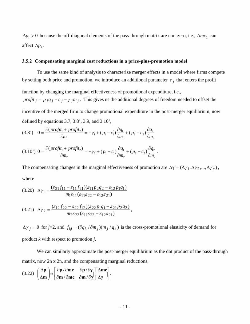
3.5.2 Compensating marginal cost reductions in a price-plus-promotion model

To use the same kind of analysis to characterize merger effects in a model where firms compete by setting both price and promotion, we introduce an additional parameter jγ that enters the profit

function by changing the marginal effectiveness of promotional expenditure, i.e.,

jjjjjj mcqpprofit γ−−= . This gives us the additional degrees of freedom needed to offset the

incentive of the merged firm to change promotional expenditure in the post-merger equilibrium, now

defined by equations 3.7, 3.8’, 3.9, and 3.10’,

(3.8’) 1

2'22

1

1'111

1

21 )()()(0mqcp

mqcp

mprofitprofit

∂∂

−+∂∂

−+−=∂+∂

= γ

(3.10’) 2

2'22

2

1'112

2

21 )()()(0mqcp

mqcp

mprofitprofit

∂∂

−+∂∂

−+−=∂+∂

= γ .

The compensating changes in the marginal effectiveness of promotion are ),...,,(' 21 nγγγ ∆∆∆=∆γ ,

where

(3.20) )(

))((

21122211111

11122211211111211 εεεεε

εεεεγ

−−−

=∆m

qpqpff

(3.21) )(

))((

21122211222

22211122122222122 εεεεε

εεεεγ

−−−

=∆m

qpqpff ,

0=∆ jγ for j>2, and )/)(/( kjjkkj qmmqf ∂∂= is the cross-promotional elasticity of demand for

product k with respect to promotion j.

We can similarly approximate the post-merger equilibrium as the dot product of the pass-through

matrix, now 2n x 2n, and the compensating marginal reductions,

(3.22) ⎥⎦

⎤⎢⎣

⎡∆∆

⎥⎦

⎤⎢⎣

⎡∂∂∂∂∂∂∂∂

≈⎟⎟⎠

⎞⎜⎜⎝

⎛∆∆

γmc

γmmcmγpmcp

mp

////

.

- 12 -

In equation (3.22), mc∆ is defined the same as in the price-only model because the first-order conditions

for price, equations (3.7) and (3.9), are unaffected by the presence of promotional expenditure.

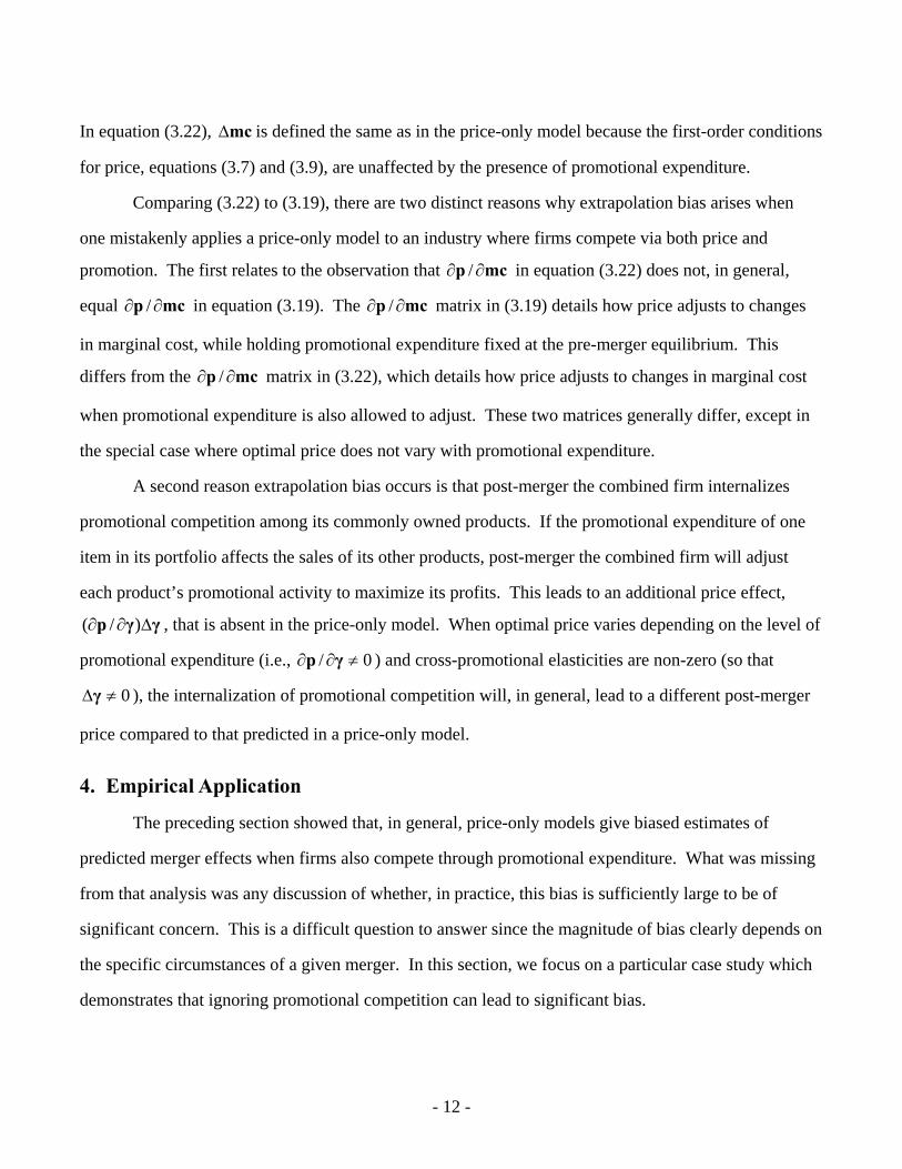
Comparing (3.22) to (3.19), there are two distinct reasons why extrapolation bias arises when

one mistakenly applies a price-only model to an industry where firms compete via both price and

promotion. The first relates to the observation that mcp ∂∂ / in equation (3.22) does not, in general,

equal mcp ∂∂ / in equation (3.19). The mcp ∂∂ / matrix in (3.19) details how price adjusts to changes

in marginal cost, while holding promotional expenditure fixed at the pre-merger equilibrium. This

differs from the mcp ∂∂ / matrix in (3.22), which details how price adjusts to changes in marginal cost

when promotional expenditure is also allowed to adjust. These two matrices generally differ, except in

the special case where optimal price does not vary with promotional expenditure.

A second reason extrapolation bias occurs is that post-merger the combined firm internalizes

promotional competition among its commonly owned products. If the promotional expenditure of one

item in its portfolio affects the sales of its other products, post-merger the combined firm will adjust

each product’s promotional activity to maximize its profits. This leads to an additional price effect,

γγp ∆∂∂ )/( , that is absent in the price-only model. When optimal price varies depending on the level of

promotional expenditure (i.e., 0/ ≠∂∂ γp ) and cross-promotional elasticities are non-zero (so that

0≠∆γ ), the internalization of promotional competition will, in general, lead to a different post-merger

price compared to that predicted in a price-only model.

4. Empirical Application

The preceding section showed that, in general, price-only models give biased estimates of

predicted merger effects when firms also compete through promotional expenditure. What was missing

from that analysis was any discussion of whether, in practice, this bias is sufficiently large to be of

significant concern. This is a difficult question to answer since the magnitude of bias clearly depends on

the specific circumstances of a given merger. In this section, we focus on a particular case study which

demonstrates that ignoring promotional competition can lead to significant bias.

- 13 -

The empirical application analyzes the super-premium ice cream industry, which was the focus

of a recent antitrust investigation by the Federal Trade Commission that culminated in a challenge to

Nestlé’s proposed acquisition of Dreyer’s Ice Cream.8 The FTC’s complaint alleged that super-premium

ice cream was the relevant product market in which to analyze the proposed transaction, which was

criticized in the popular press as being too narrow.9

According to the Horizontal Merger Guidelines (1992), the relevant market in which to analyze a

merger is the smallest class of products for which a hypothetical monopolist could profitably raise price

by a small but significant amount, often taken to be a 5% price increase. This test can be implemented

by conducting a simulation exercise that predicts the price effects of a merger to monopoly. If the

simulation predicts a significant post-merger price increase then super-premium ice cream is a relevant

market. If not, the relevant market comprises a wider set of products.10

We take the two steps outlined in section 2: demand and costs are estimated from pre-merger

data, and then the model is used to forecast the effect of a merger to monopoly. To make the model

tractable, we rely upon two simplifying assumptions that have been widely employed in previous

research. First, when estimating demand we assume consumers make their purchase decisions based on

the price and promotional activity at a particular store. This allows demand to be estimated using data

from only a subset of the retailers in a given geographic area. Second, we do not explicitly model the

interplay between manufacturers and retailers. Manufacturers are the sole strategic actors in the model,

and determine both price and promotional activity. Retailers are passive actors that merely pass along

upstream changes in these variables. This modeling approach has been widely employed in the merger

simulation literature, with researchers only starting to explore alternative frameworks in which retailers

play a more strategic role (Froeb et al. 2007).

8 See the citation in footnote 5.

9 See, for instance, “FTC Screams for Antitrust” (Holman W. Jenkins, Jr., Wall Street Journal, March 12, 2003), and “The Emperors of Ice Cream” (Donald Luskin, National Review, March 6, 2003).

10 Although we only address whether this merger simulation supports the FTC’s market delineation, it is standard practice for the FTC to consider a much wider range of evidence when analyzing a prospective merger.

- 14 -

In order to conduct this product market test, we must overcome two problems. First, we do not

observe promotional expenditure, only the incidence of promotional activity. We therefore re-

parameterize the model so that it can be estimated without directly observing promotional expenditure.

Second, we do not have store-level data; instead we rely on weekly scanner data that is aggregated

across all stores in a given city-chain (e.g., the Jewel supermarket chain in Chicago in the third week in

January, 2002).11 When estimating demand with aggregate data, researchers typically rely upon a

representative store model where promotional intensity is measured as the fraction of stores on

promotion. But variation in the fraction of stores on promotion is likely to be a poor proxy for the effect

of discrete changes in promotion that occur at the individual store level, i.e., a store either promotes an

item or it does not. As one might expect by Jensen’s inequality this leads to bias in non-linear demand

models (Christen et al., 1997). To avoid such bias, we explicitly model inter-store promotional

heterogeneity and then aggregate demand across the heterogeneous stores so that our empirical model

matches the available data.

4.1 Demand Estimation

We rely upon demand estimates from a companion paper, Tenn (2006). Since demand

estimation is not the focus of this paper, we provide only a condensed description of the demand model

employed. Readers interested in a complete description of the demand estimation procedure should

refer to the companion paper.

The super-premium ice cream data from ACNielsen reports 80 weeks of sales data for 11 city-

chain combinations. Such data is often used to estimate demand to inform merger analysis, e.g., Werden

(2000). The category contains the same four brands in each of the 11 city-chains covered by the data.

To comply with confidentiality requirements, they are referred to as Brand A, B, C, and D.

The data separately reports sales for four (mutually exclusive) levels of promotional activity,

Mm∈ , where M={“No Promotion,” “Display Only,” “Feature Only,” and “Feature & Display”}. A

11 A confidentiality agreement with ACNielsen prohibits retailer names from being revealed. This example does not

indicate whether the dataset employed contains the Jewel supermarket chain in Chicago.

- 15 -

display is a secondary sales location, e.g., at the end of an aisle, that draws special attention to a

particular product. A feature is an advertisement appearing in a newspaper, circular, or flyer. Note that

“No Promotion” includes temporary price reductions so long as they are not accompanied by a feature or

a display. Coupons are not reported in the data. We do not believe, however, that coupons are common

for super-premium ice cream.

Super-premium ice cream begins to degrade in as little as a few weeks after it is brought home

from the store. This mitigates the well known problem of strategic hording behavior by consumers, who

wait until price drops to purchase the good (Hendel and Nevo, forthcoming).

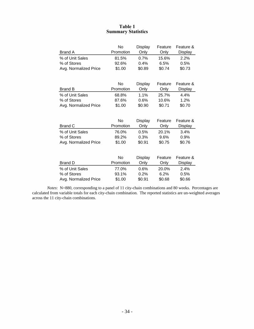
Table 1 presents summary statistics for each brand. A significant fraction of super-premium ice

cream is sold on promotion, with “Feature Only” the most common form of promotional activity. Unit

sales are high relative to the fraction of stores on promotion for each type of elevated promotional

activity (i.e., excluding “No Promotion”). In part, this is due to the price reduction that typically occurs

when a brand is on promotion; each brand’s price is approximately 10% lower when on “Display Only”

and 30% lower when on either “Feature Only” or “Feature & Display.”

In every time period t, each consumer i purchases that item which generates the highest utility.

The choices are the set of currently available products tJ or the “outside good.” We normalize the

utility derived from purchasing the outside good to a mean utility of zero, titiU 00 ω= , where ti0ω is

i.i.d. Type I Extreme Value (Gumbel). For the remaining choices, consumer i’s utility for product j during week t is determined by its promotional activity Mmijt ∈ , price ijtp , a set of product

characteristics ijtX that has an associated vector of random coefficients iν , a set of additional controls

jtZ , and an error term ijtω that is distributed i.i.d. Type I Extreme Value.12

(4.1) ijtjtiijtijtijtmijtm

ijt ZXpU ωγνβµ ++++=

Product characteristics ijtX include a set of dummy variables for each brand, price ijtp , and dummy

variables for “Display Only,” “Feature Only” and “Feature & Display.” Control variables jtZ consist

12 City-chain subscripts are dropped from the control variables for ease of notation.

- 16 -

of brand fixed effects for each city-chain combination, a fourth order time trend, the number of products

available in the category, and the square of this variable.

The model specifies a separate intercept mµ and price coefficient mβ for each type of

promotional activity Mm∈ . This specification allows the data to determine whether promotion makes

demand less or more elastic which, in turn, determines whether optimal promotion increases or

decreases with price. In the appendix, we detail three canonical demand specifications of promotion in a

logit choice model. In the first two models, we consider the implications of letting promotional activity

influence the intercept and price coefficient in the utility function. Our empirical specification

accommodates both possibilities. The third model we consider in the appendix is the case when

promotional activity changes consumer awareness of the existence of a product. This possibility is

excluded from the empirical specification due to a lack of observable variation which could be used to

identify how promotions affect consumer choice sets. While variation in the type of promotional

activity identifies the intercept of the utility function, and price variation within each type of promotion

identifies the price coefficient, the dataset contains no information regarding the fraction of consumers

who are aware that a product exists. Identification of this effect would be entirely spurious, resulting

from nonlinearities in the functional form employed. As such, we do not incorporate this possible effect

into the empirical specification.

The model accommodates heterogeneity in consumer preferences through random coefficients

iν . This vector is mean-zero and i.i.d. Normally distributed with a block diagonal variance matrix

]0

0[

2

1V

VV = . Denote the probability distribution function of iν by );( Viνφ . 1V corresponds to the

brand dummy variables contained in ijtX (the fixed characteristics), while 2V corresponds to the

remaining price and promotion variables (the variable characteristics). No restrictions are imposed on

1V and 2V apart from the requirement that each be a symmetric positive semi-definite matrix.

Aggregate scanner datasets do not report any information regarding the distribution of prices

across stores with the same promotional activity. Given this data limitation, we assume that stores with

the same promotional activity for a given product all charge the same price.

- 17 -

(4.2) mmipp ijtmjtijt =∀= :,

The model accommodates heterogeneous promotional activity across stores. Store type Gg ∈ is

a vector that contains each product’s promotional activity. Consumer i in week t visits store type

tJjijtit mg ∈= }{ . Denote the element of itg that corresponds to product j by )( itj gm . Product

characteristics ijtX are written as )( itjt gX since the included variables vary only by store type g. This

allows the utility function to be re-written as follows.

(4.3) ijtjtiitjtitgjm

jtitgjmitgjm

ijt ZgXpU ωγνβµ ++++= )()()()(

All stores are identical apart from heterogeneity in price and promotional activity. In addition,

each consumer is randomly matched to a store. This allows integration over the distribution of random

coefficients iν for the subset of consumers who visit a given store type g.

Each consumer i purchases product j only when that item generates the highest utility from

among the available choices. The distributional assumptions provided above imply the following for gjtq , unit sales for product j across all stores that have promotional activity g during week t.

(4.4) ii

tJk

ktZigktXgkmktpgkmgkm

jtZigjtXgjm

jtpgjmgjm

gtgjt dV

e

eQq ννφπγνβµ

γνβµ

);(

1])()()()([

])()()()(

[

∫∑∈

+++

+++

+

=

Q represents the total number of consumers in the market, while gtπ is the fraction of consumers who

visit store type g in week t.

In the super-premium ice cream category each brand’s UPCs represent a different flavor, with a

particular flavor rarely available for more than one brand (e.g., “Chunky Monkey” is available only for

the Ben & Jerry’s brand). The large number of idiosyncratic flavors limits the usefulness of this

characteristic for estimating substitution patterns. Other meaningful characteristics are common across

UPCs for a given brand; each brand’s UPCs share the same brand image and, within any given store,

they are identically priced and promoted. As a result, each variable in (4.4) that has a product j subscript

is identical across products within the same brand. Therefore, for each brand Bb∈ we aggregate unit

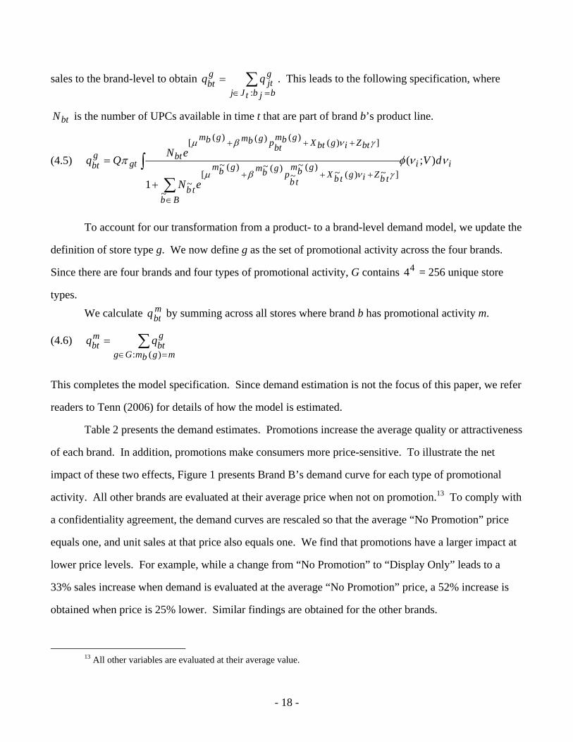
- 18 -

sales to the brand-level to obtain ∑=∈

=bjbtJj

gjt

gbt qq

:. This leads to the following specification, where

btN is the number of UPCs available in time t that are part of brand b’s product line.

(4.5) ii

Bb

tbZigtbXgbm

tbp

gbmgbm

tb

btZigbtXgbmbtpgbmgbm

btgt

gbt dV

eN

eNQq ννφπ

γνβµ

γνβµ

);(

1~

]~)(~)(~~

)(~)(~[

~

])()()()([

∫∑∈

+++

+++

+

=

To account for our transformation from a product- to a brand-level demand model, we update the

definition of store type g. We now define g as the set of promotional activity across the four brands.

Since there are four brands and four types of promotional activity, G contains 44 = 256 unique store

types. We calculate m

btq by summing across all stores where brand b has promotional activity m.

(4.6) ∑=∈

=mgbmGg

gbt

mbt qq

)(:

This completes the model specification. Since demand estimation is not the focus of this paper, we refer

readers to Tenn (2006) for details of how the model is estimated.

Table 2 presents the demand estimates. Promotions increase the average quality or attractiveness

of each brand. In addition, promotions make consumers more price-sensitive. To illustrate the net

impact of these two effects, Figure 1 presents Brand B’s demand curve for each type of promotional

activity. All other brands are evaluated at their average price when not on promotion.13 To comply with

a confidentiality agreement, the demand curves are rescaled so that the average “No Promotion” price

equals one, and unit sales at that price also equals one. We find that promotions have a larger impact at

lower price levels. For example, while a change from “No Promotion” to “Display Only” leads to a

33% sales increase when demand is evaluated at the average “No Promotion” price, a 52% increase is

obtained when price is 25% lower. Similar findings are obtained for the other brands.

13 All other variables are evaluated at their average value.

- 19 -

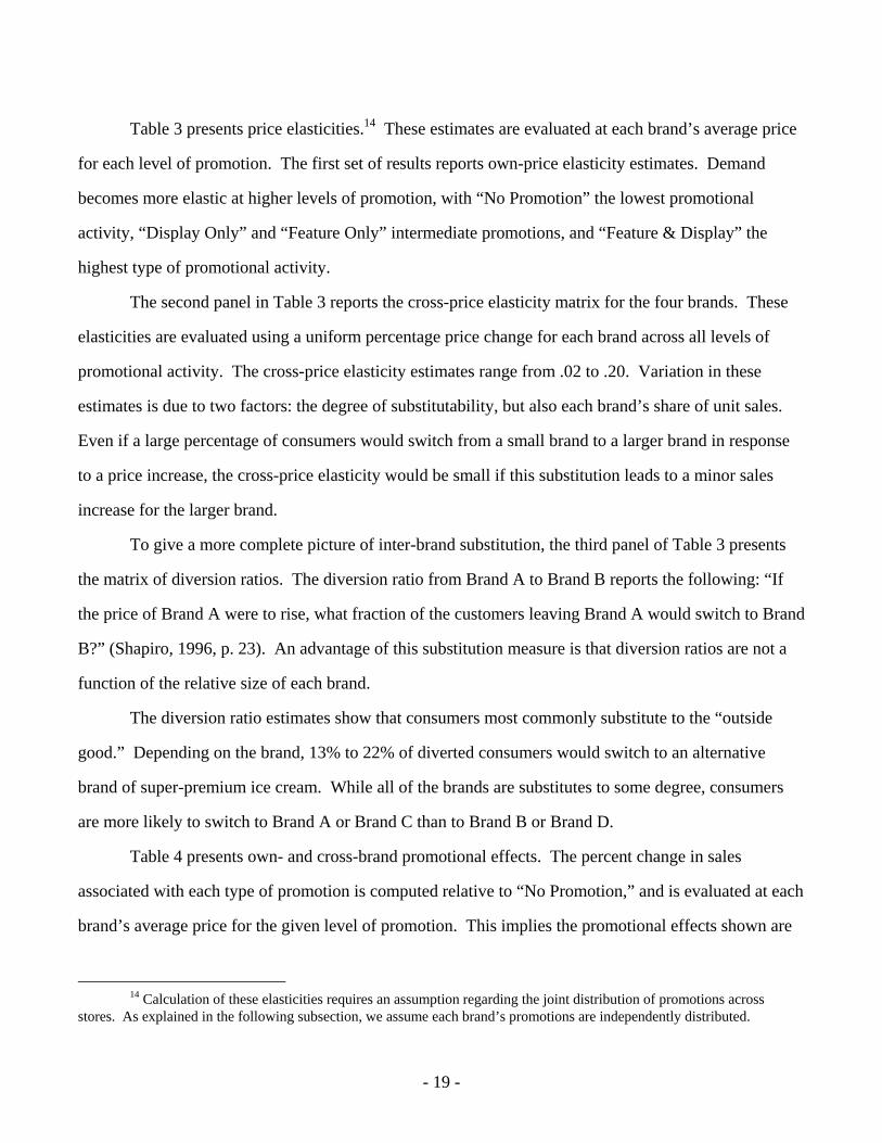
Table 3 presents price elasticities.14 These estimates are evaluated at each brand’s average price

for each level of promotion. The first set of results reports own-price elasticity estimates. Demand

becomes more elastic at higher levels of promotion, with “No Promotion” the lowest promotional

activity, “Display Only” and “Feature Only” intermediate promotions, and “Feature & Display” the

highest type of promotional activity.

The second panel in Table 3 reports the cross-price elasticity matrix for the four brands. These

elasticities are evaluated using a uniform percentage price change for each brand across all levels of

promotional activity. The cross-price elasticity estimates range from .02 to .20. Variation in these

estimates is due to two factors: the degree of substitutability, but also each brand’s share of unit sales.

Even if a large percentage of consumers would switch from a small brand to a larger brand in response

to a price increase, the cross-price elasticity would be small if this substitution leads to a minor sales

increase for the larger brand.

To give a more complete picture of inter-brand substitution, the third panel of Table 3 presents

the matrix of diversion ratios. The diversion ratio from Brand A to Brand B reports the following: “If

the price of Brand A were to rise, what fraction of the customers leaving Brand A would switch to Brand

B?” (Shapiro, 1996, p. 23). An advantage of this substitution measure is that diversion ratios are not a

function of the relative size of each brand.

The diversion ratio estimates show that consumers most commonly substitute to the “outside

good.” Depending on the brand, 13% to 22% of diverted consumers would switch to an alternative

brand of super-premium ice cream. While all of the brands are substitutes to some degree, consumers

are more likely to switch to Brand A or Brand C than to Brand B or Brand D.

Table 4 presents own- and cross-brand promotional effects. The percent change in sales

associated with each type of promotion is computed relative to “No Promotion,” and is evaluated at each

brand’s average price for the given level of promotion. This implies the promotional effects shown are

14 Calculation of these elasticities requires an assumption regarding the joint distribution of promotions across

stores. As explained in the following subsection, we assume each brand’s promotions are independently distributed.

- 20 -

the combined impact of being on promotion and undergoing the average price reduction for that

promotion. Across all four brands, promotional activity leads to a significant sales increase for the

brand undertaking the promotion, with “Display Only” having the smallest effect and “Feature and

Display” the largest impact.

In addition, we find that a promotion by one brand reduces the sales of the other brands. In the

merger simulations reported in the following subsection, the merged firm internalizes these cross-brand

promotional effects. Just as the internalization of price competition among commonly owned products

leads to a post-merger price increase, the internalization of promotional competition leads to a reduction

in post-merger promotional activity.

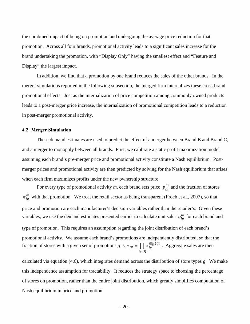
4.2 Merger Simulation

These demand estimates are used to predict the effect of a merger between Brand B and Brand C,

and a merger to monopoly between all brands. First, we calibrate a static profit maximization model

assuming each brand’s pre-merger price and promotional activity constitute a Nash equilibrium. Post-

merger prices and promotional activity are then predicted by solving for the Nash equilibrium that arises

when each firm maximizes profits under the new ownership structure. For every type of promotional activity m, each brand sets price m

btp and the fraction of stores mbtπ with that promotion. We treat the retail sector as being transparent (Froeb et al., 2007), so that

price and promotion are each manufacturer’s decision variables rather than the retailer’s. Given these variables, we use the demand estimates presented earlier to calculate unit sales m

btq for each brand and

type of promotion. This requires an assumption regarding the joint distribution of each brand’s

promotional activity. We assume each brand’s promotions are independently distributed, so that the fraction of stores with a given set of promotions g is ∏

∈=

Bb

gbmbtgt

)(ππ . Aggregate sales are then

calculated via equation (4.6), which integrates demand across the distribution of store types g. We make

this independence assumption for tractability. It reduces the strategy space to choosing the percentage

of stores on promotion, rather than the entire joint distribution, which greatly simplifies computation of

Nash equilibrium in price and promotion.

- 21 -

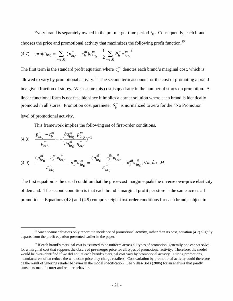
Every brand is separately owned in the pre-merger time period 0t . Consequently, each brand

chooses the price and promotional activity that maximizes the following profit function.15

(4.7) ∑ ∑∈ ∈

−−=Mm Mm

mbt

mb

mbt

mb

mbtbt qcpprofit

2

0000 21)( πθ

The first term is the standard profit equation where mbc denotes each brand’s marginal cost, which is

allowed to vary by promotional activity.16 The second term accounts for the cost of promoting a brand

in a given fraction of stores. We assume this cost is quadratic in the number of stores on promotion. A

linear functional form is not feasible since it implies a corner solution where each brand is identically promoted in all stores. Promotion cost parameter m

bθ is normalized to zero for the “No Promotion”

level of promotional activity.

This framework implies the following set of first-order conditions.

(4.8) 1

0

0

0

0

0

0 )( −

∂

∂−=

−

mbt

mbt

mbt

mbt

mbt

mb

mbt

q

p

p

q

p

cp

(4.9) Mmmqcpqcp

mbt

mbm

bt

mbt

mb

mbtm

btmbm

bt

mbt

mb

mbt

∈∀−−

=−−

~,,)()( ~

0

~~

0

~

0

~~

00

0

00 πθπ

πθπ

The first equation is the usual condition that the price-cost margin equals the inverse own-price elasticity

of demand. The second condition is that each brand’s marginal profit per store is the same across all

promotions. Equations (4.8) and (4.9) comprise eight first-order conditions for each brand, subject to

15 Since scanner datasets only report the incidence of promotional activity, rather than its cost, equation (4.7) slightly

departs from the profit equation presented earlier in the paper.

16 If each brand’s marginal cost is assumed to be uniform across all types of promotion, generally one cannot solve for a marginal cost that supports the observed pre-merger price for all types of promotional activity. Therefore, the model would be over-identified if we did not let each brand’s marginal cost vary by promotional activity. During promotions, manufacturers often reduce the wholesale price they charge retailers. Cost variation by promotional activity could therefore be the result of ignoring retailer behavior in the model specification. See Villas-Boas (2006) for an analysis that jointly considers manufacturer and retailer behavior.

- 22 -

the constraint 10=∑

∈Mm

mbtπ . Using data on pre-merger price and promotional activity, these first-order

conditions exactly identify mbc and m

bθ for each brand and type of promotion.

The final step in the merger simulation analysis is to calculate the post-merger Nash equilibrium.

To simulate a merger between Brand B and Brand C, we solve for each brand’s price and promotional

activity that satisfy the new set of first-order conditions that arises when Brand B and Brand C maximize

their joint profits. The first-order conditions for Brand A and Brand D remain unchanged, although their

price and promotion levels adjust in response to changes in the other two brands’ prices and promotions.

Panel A of Table 5 presents the predicted impact of a merger between Brand B and Brand C.

Two types of price increases occur following the transaction. First, the price associated with each type

of promotional activity rises. Second, the fraction of stores on promotion is reduced, with a counterpart

increase in the number of stores on “No Promotion.” Since the non-promoted price is higher, this

composition shift in promotional activity leads to an increase in average price.

Recall that consumers are more likely to substitute from Brand B to Brand C than from Brand C

to Brand B. Due to this asymmetry, the predicted price increase is larger for Brand B. Brand B’s post-

merger price rises by 5.4% to 6.7%, depending on the level of promotional activity. In addition, there is

a 22.2% reduction in the fraction of stores where Brand B is on promotion. These two effects lead to an

8.1% overall price increase. The price increase and promotional activity reduction for Brand C are

substantially smaller. The fraction of stores on promotion declines by 8.3%, with an overall price

increase of 2.4%.

To assess the empirical support for the FTC’s proposed market delineation, panel B of Table 5

reports results from a second merger simulation that predicts the impact of a merger to monopoly. As

expected, merger to monopoly leads to significantly higher post-merger price increases than a merger

between only Brand B and Brand C. Apart from this difference in scale, however, we observe similar

merger effects; not only does price rise (9.4% to 19.9%, depending on the brand), but also the fraction of

stores on promotion significantly declines (26.9% to 41.1%, depending on the brand).

- 23 -

In section 3.5, we detailed two reasons why promotional activity may change in the post-merger

equilibrium. First, optimal promotional activity may vary with price. As the combined firm internalizes

price competition across its commonly owned products, promotional activity will also adjust. In

addition, post-merger the combined firm internalizes promotional competition across its commonly

owned products. If a promotion for one item reduces the sales of other products in the combined firm’s

portfolio, this effect is internalized post-merger leading to reduced promotional activity.

We conduct an additional merger simulation exercise to determine which of these two factors is

the primary reason the model predicts a post-merger decline in promotions. In this simulation, we allow

promotional activity to adjust post-merger but fix price at the pre-merger equilibrium. The predicted

post-merger reductions in the fraction of stores on promotion are extremely similar to the results

reported in Table 5, where both price and promotion are allowed to change post-merger. This shows the

post-merger decline in promotional activity is almost entirely due to the internalization of promotional

competition between the combined firm’s commonly owned products.

Next, we compare the merger simulation results reported in Table 5 to two alternative

specifications. The first uses the same demand estimates, but promotional activity is held fixed during

the merger simulation. In the second alternative specification promotional activity is entirely ignored,

both when estimating demand and when simulating the post-merger equilibrium.17 Promotional activity

and price reductions are correlated, which leads to omitted variables bias. If promotions are ignored

when estimating demand, price reductions appear to have a larger influence on sales than is actually the

case. While the own-price elasticities in panel B of Table 3 range from -1.61 to -1.90, depending on the

brand, the own-price elasticities increase in magnitude to -2.42 to -2.73 when promotional activity is

omitted from the demand model.18 All else equal, more elastic demand leads to smaller post-merger

price increases.

17 Weiskopf (2000) also analyzes whether inclusion of promotional activity affects merger simulation results. While

Weiskopf obtains similar findings regardless of whether promotions are included in the demand model, he does not include promotional activity as a control variable in the merger simulation analysis.

18 The full matrix of elasticity and diversion ratio estimates when promotional activity is omitted from the demand model is available upon request.

- 24 -

A comparison of the three sets of results shown in Table 6 reveals that larger post-merger price

effects are obtained when promotions are controlled for both in the demand model and when simulating

the merger. Panel A of Table 6 corresponds to a merger between Brand B and Brand C. While the

predicted price increase for Brand B is 8.1% when promotions are fully incorporated into the analysis,

the effect declines to 6.3% when promotions are held fixed when solving for the post-merger

equilibrium. The price increase is only 3.3% when promotions are also ignored in the demand

estimation procedure. Similar results are obtained for Brand C; the price effects decline from 2.4%

when promotions are fully incorporated in the analysis to only 1.1% when promotional activity is

ignored (both when estimating demand and in the merger simulation itself).

We decompose the bias from not fully incorporating promotions into the merger simulation

analysis. For Brand B, 64% of the difference in the predicted price increase is due to “estimation bias”

(promotions are omitted from the demand model), while the remaining 36% is due to “extrapolation

bias” (promotional activity is held constant when solving for the post-merger equilibrium). The

decomposition for Brand C is similar; estimation bias accounts for 72% of the difference, while

extrapolation bias represents the remaining 28%.

Panel B of Table 6 reports results from a second set of merger simulations where we predict the

impact of a merger to monopoly. As before, our findings illustrate the importance of fully controlling

for promotional activity, both in demand estimation and in the merger simulation itself. When

promotions are excluded from the demand model, the own-price elasticity estimates are biased upward

(too elastic). This estimation bias leads to smaller predicted price increases. The price change for Brand

A and Brand C is only 4.4% and 4.1%, respectively, although substantial price increases are predicted

for the other two brands. The price increase for the category is 4.9%, which we construct by weighting

each brand’s price increase by the average of its pre- and post-merger unit sales. This is slightly less

than the 5% cutoff typically used to delineate markets, i.e., if the hypothetical monopolist raises price by

at least 5% then the candidate products are deemed an antitrust “market.”

Larger price increases are predicted when promotions are included in the demand model, but are

held fixed in the merger simulation. The price increases for Brand A and Brand C are 8.9% and 8.1%,

- 25 -

respectively, with larger predicted effects for the other two brands. With a category price increase of

10.0%, these results support separate delineation of a super-premium ice cream market.

The FTC’s proposed market delineation is also supported when promotional activity is included

as a control variable in the merger simulation exercise. Each brand’s predicted price increase is quite

substantial, ranging from 9.4% to 19.9%. As before, we decompose the bias from not fully

incorporating promotions into the merger simulation analysis. Both estimation and extrapolation bias

are significant; approximately three-fourths of the difference between the alternative specifications is

due to estimation bias, with the remaining one-fourth due to extrapolation bias.

To summarize, the strongest support for a super-premium ice cream market is obtained when

promotions are not only controlled for in the demand model, but also in the merger simulation analysis.

Excluding promotions from the demand model leads to estimation bias, while not allowing post-merger

promotional activity to adjust leads to extrapolation bias. This example illustrates how these biases not

only affect the size of predicted merger effects, but can potentially impact delineation of the relevant

antitrust market.

We conclude with a brief discussion of compensating marginal cost reductions, which are a

useful way to assess whether the efficiencies claimed by the merging parties are sufficient to offset the

price effects of the merger. For the price-plus-promotion model, panel A of Table 7 reports the changes

in marginal production cost and marginal promotion cost necessary to preserve the pre-merger

equilibrium. Large efficiencies are required to offset the merger effects. For example, for the merger

between Brand B and Brand C, Brand B’s marginal production cost would have to decline by 11.3% to

15.9%, depending on the type of promotion, while its marginal promotion cost would have to decline by

.8% to 3.9% (for the reasons provided earlier, the required efficiencies for Brand C are substantially

smaller). As expected, the required efficiencies to offset a merger to monopoly are larger than for a

merger between only Brand B and Brand C. Depending on the brand and type of promotion, marginal

production costs would have to decline by as much as 42.7%, while marginal promotion costs would

have to decline by as much as 13.0%.

- 26 -

We compare the compensating marginal cost reductions in the price-plus-promotion model to

those for the price-only model, which are reported in Panel B of Table 7. The price-only model under-

predicts the efficiencies required to offset the merger effect. This is analogous to our earlier finding that

the price-only model under-predicts the post-merger price increase. For example, in a merger between

Brand B and Brand C, Brand B’s marginal production cost would have to decline by only 6.0% in the

price-only model to maintain the pre-merger equilibrium. This is approximately half the cost decline

required in the price-plus-promotion model. In our application, reliance on a price-only model could

lead antitrust authorities to conclude that claimed (and verified) merger efficiencies are sufficient to

offset the anticompetitive impact of a merger, when in fact much larger efficiencies might be required.

5. Conclusion

Models necessarily simplify the real world. What we want to know is whether the

simplifications employed bias the model predictions. In this paper, we analyze mergers in industries

where firms compete by setting both price and promotion. Our investigation identifies two types of bias

in merger models that ignore non-price competition. Estimation bias is a type of omitted variables bias.

If promotions are ignored when estimating demand, price elasticity estimates will be biased since they

partially reflect correlated promotional activity. Extrapolation bias occurs when price-only models

mistakenly hold promotion fixed at the pre-merger equilibrium. This not only leads to a biased forecast

of post-merger promotional activity, but also a biased forecast of post-merger prices when pricing and

promotion decisions are inter-dependent.

Extrapolation and estimation bias arises when optimal price varies with promotional activity (and

vice-versa). This is the case in the super-premium ice cream industry, the focus of our empirical

analysis. Pricing and promotion decisions are jointly determined in this industry, as is evident by the

fact that most price variation occurs simultaneously with variation in promotional activity (i.e., products

typically have price reductions in those weeks where they are on promotion via a feature advertisement

or an in-store display). Analysis of the super-premium ice cream industry confirms that a price-only

model performs poorly when price and promotional activity are jointly determined; estimation and

- 27 -

extrapolation bias both cause the price-only model to under-predict the post-merger price increase. Our

analysis demonstrates the potential for biased results in price-only merger models. Additional research

is needed to determine whether models that explicitly account for non-price competition can better

predict the effect of real world events, such as consummated mergers. For mergers that were blocked by

the antitrust authorities, however, testing the sensitivity of models to alternative assumptions of how

firms compete, like the exercise in this paper, may be the next best alternative.

- 28 -

References Berry, Steven T. (1994), “Estimating Discrete-Choice Models of Product Differentiation,” RAND

Journal of Economics, 25(2):242-62.

Christen, Markus, Sachin Gupta, John C. Porter, Richard Staelin, and Dick R. Wittink (1997), “Using Market-Level Data to Understand Promotion Effects in a Nonlinear Model,” Journal of Marketing Research, 34(3):322-34.

Crooke, Philip, Luke Froeb, Steven Tschantz, and Gregory J. Werden (1999), “Effects of Assumed Demand Form on Simulated Postmerger Equilibria,” Review of Industrial Organization, 15(3):205-17.

Dorfman, Robert, and Peter O. Steiner (1954), “Optimal Advertising and Optimal Quality,” American Economic Review, 44(5):826-36.

Federal Trade Commission (2005), “Estimating the Price Effects of Mergers and Concentration in the Petroleum Industry: An Evaluation of Recent Learning,” transcript from hearings on January 14-15, 2005. Available at http://www.ftc.gov/ftc/workshops/oilmergers.

Froeb, Luke, Steven Tschantz, and Philip Crooke (2003), “Bertrand Competition with Capacity Constraints: Mergers among Parking Lots,” Journal of Econometrics, 113(1):49-67.

Froeb, Luke, Steven Tschantz, and Gregory Werden (2005), “Pass-Through Rates and the Price Effects of Mergers,” International Journal of Industrial Organization, 23(9/10):703-15.

Froeb, Luke, Steven Tschantz, and Gregory Werden (2007), “Vertical Restraints and the Effects of Upstream Horizontal Mergers,” in Vivek Ghosal and Johann Stennek, eds., The Political Economy of Antitrust. Amsterdam: North-Holland Publishing.

Froeb, Luke M., and Gregory J. Werden (1998), “A Robust Test for Consumer Welfare Enhancing Mergers Among Sellers of a Homogeneous Product,” Economics Letters, 58(3):367-69.

Gandhi, Amit, Luke Froeb, Steven Tschantz, and Gregory Werden (Forthcoming), “Post-Merger Product Repositioning,” Journal of Industrial Economics.

Hadeishi, Hajime, and Dave Schmidt (2004), “The Price Effects of a Merger of Complements: The Case of Peanut Butter and Jelly,” Working Paper, Federal Trade Commission.

Hausman, Jerry, Gregory Leonard, and Douglas J. Zona (1994), “Competitive Analysis with Differentiated Products,” Annales d’Economie et Statistique, 34(2):159-80.

Hendel, Igal, and Aviv Nevo (Forthcoming), “Measuring the Implications of Sales and Consumer Stockpiling Behavior,” Econometrica.

Hosken, Daniel, Daniel O’Brien, David Scheffman, and Michael Vita (2005), “Demand System Estimation and its Application to Horizontal Merger Analysis,” Appendix IV in Econometrics: Legal, Practical, and Technical Issues, John D. Harkrider (ed.), ABA Section of Antitrust Law.

Kim, Dae-Wook, and Christopher R. Knittel (2006), “Biases in Static Oligopoly Models? Evidence from the California Electricity Market,” Journal of Industrial Economics, 54(4):451-70.

- 29 -

McCarthy, E. Jerome (1981), Basic Marketing: A Managerial Approach. Homewood, IL: Richard D. Irwin.

Nevo, Aviv (2000), “Mergers with Differentiated Products: The Case of the Ready-to-Eat Cereal Industry,” RAND Journal of Economics, 31(3):395-421.

O’Brien, Daniel P., and Greg Shaffer (2005), “Bargaining, Bundling, and Clout: The Portfolio Effects of Horizontal Mergers,” RAND Journal of Economics, 36(3):573-95.

Peters, Craig (2006), “Evaluating the Performance of Merger Simulation: Evidence from the U.S. Airline Industry,” Journal of Law and Economics, 49(2):627-49.

Pinske, Joris, and Margaret E. Slade (2004), “Mergers, Brand Competition, and the Price of a Pint,” European Economic Review, 48(3):617-43.

Schinkel, Maarten Pieter, Marie Christine Goppelsroeder, and Jan Tuinstra (2006), “Quantifying the Scope for Efficiency Defense in Merger Control: The Werden-Froeb-Index,” Amsterdam Center for Law & Economics Working Paper No. 2006-10.

Shapiro, Carl (1996), “Mergers with Differentiated Products,” Antitrust, 10(2):23-30.

U.S. Department of Justice and Federal Trade Commission (1992), Horizontal Merger Guidelines. Available at http://www.usdoj.gov/atr/public/guidelines/horiz_book/hmg1.html.

Tschantz, Steven, Philip Crooke, and Luke Froeb (2000), “Mergers in Sealed versus Oral Auctions,” International Journal of the Economics of Business, 7(2):201-12.

Tenn, Steven (2006), “Avoiding Aggregation Bias in Demand Estimation: A Multivariate Promotional Disaggregation Approach,” Quantitative Marketing and Economics, 4(4):383-405.

Villas-Boas, Sofia (2006), “Vertical Contracts between Manufacturers and Retailers: Inference with Limited Data,” Working Paper, UC Berkeley.

Weinberg, Matthew (2005), “An Evaluation of Merger Simulations,” Working Paper, Princeton University.

Weiskopf, David A. (2000), “The Impact of Omitting Promotion Variables on Simulation Experiments,” International Journal of the Economics of Business, 7(2):159-66.

Werden, Gregory J. (1996), “A Robust Test for Consumer Welfare Enhancing Mergers Among Sellers of Differentiated Products,” Journal of Industrial Economics, 44(4):409-13.

Werden, Gregory J. (2000), “Expert Report in United States v. Interstate Bakeries Corp. and Continental Baking Co.,” International Journal of the Economics of Business, 7(2):139-48.

Werden, Gregory J., and Luke M. Froeb (1994), “The Effects of Mergers in Differentiated Products Industries: Logit Demand and Merger Policy,” Journal of Law, Economics, and Organization, 10(2):407-26.

Werden, Gregory J., Luke M. Froeb, and David T. Scheffman (2004), “A Daubert Discipline for Merger Simulation,” Antitrust, 18(3):89-95.

- 30 -

6. APPENDIX: Three Structural Demand Models of Price and Promotion

In section 3 we show that the role that promotion plays in merger analysis depends, to a large

extent, on the relationship between optimal promotion and price which, in turn, depends on how

promotion affects demand. To better understand how to construct an empirical model of promotion, we

explore three ways in which promotional activity might influence demand. We find that if promotion

serves only to inform consumers of the existence of a good, then optimal promotion is independent of

price. If promotion increases the mean quality of a good, then promotion makes demand less elastic,

and optimal promotion increases with price. On the other hand, if promotion increases the price-

sensitivity of consumers, then promotion makes demand more elastic, and optimal promotion decreases

with price. These three cases correspond to a zero, negative, and positive marginal cost adjustment,

respectively (as defined in section 3).

6.1 Benchmark price-only model

The price-only model to which the price-plus-promotion models are compared is the “antitrust

logit model” (Werden and Froeb, 1994), where consumer behavior is characterized by a simple logit

choice model and firm behavior is characterized by Nash equilibrium in prices with constant marginal

cost of production.

Each consumer i purchases that item which generates the highest indirect utility. The choices are

the set of currently available products J or the “outside good.” Consumer i’s utility for product j is determined by ijjjij pU ωβµ ++= , where 0<β measures consumer price-sensitivity and ijω is i.i.d.

Type I Extreme Value (Gumbel). We normalize the utility derived from purchasing the outside good to

a mean utility of zero )0( 00 == pµ , so that 00 iiU ω= . The fraction of consumers who purchase

product j has the familiar logit form,

(6.1) ∑∈

+

+

+=

Jk

kpk

jpjj

ees βµ

βµ

1,

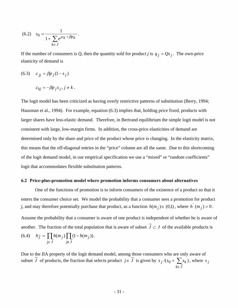
while the fraction of consumers who purchase the outside good is

- 31 -

(6.2) ∑∈

++=

Jk

kpkes

βµ11

0 .

If the number of consumers is Q, then the quantity sold for product j is jj Qsq = . The own-price elasticity of demand is

(6.3) )1( jjjj sp −= βε

kjsp jjkj ≠−= ,βε .

The logit model has been criticized as having overly restrictive patterns of substitution (Berry, 1994;

Hausman et al., 1994). For example, equation (6.3) implies that, holding price fixed, products with

larger shares have less-elastic demand. Therefore, in Bertrand equilibrium the simple logit model is not

consistent with large, low-margin firms. In addition, the cross-price elasticities of demand are

determined only by the share and price of the product whose price is changing. In the elasticity matrix,

this means that the off-diagonal entries in the “price” column are all the same. Due to this shortcoming

of the logit demand model, in our empirical specification we use a “mixed” or “random coefficients”

logit that accommodates flexible substitution patterns.

6.2 Price-plus-promotion model where promotion informs consumers about alternatives

One of the functions of promotion is to inform consumers of the existence of a product so that it

enters the consumer choice set. We model the probability that a consumer sees a promotion for product j, and may therefore potentially purchase that product, as a function )1,0()( ∈jmh , where 0)(' >jmh .

Assume the probability that a consumer is aware of one product is independent of whether he is aware of

another. The fraction of the total population that is aware of subset JJ ⊂~ of the available products is

(6.4) ))(1()(~~

~ ∏∏∉∈

−=Jj

jJj

jJ mhmhh .

Due to the IIA property of the logit demand model, among those consumers who are only aware of subset J~ of products, the fraction that selects product Jj ~∈ is given by )/(

~0 ∑∈

+Jk

kj sss , where js

- 32 -

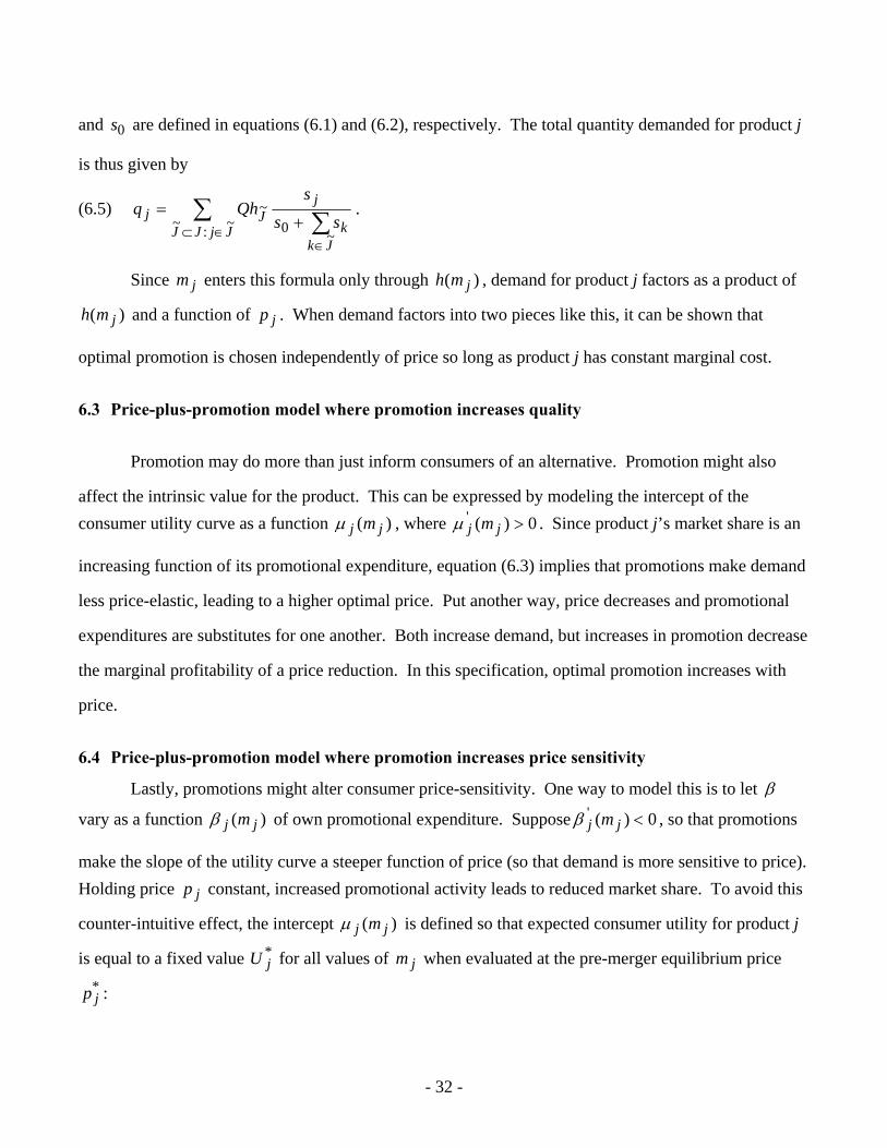
and 0s are defined in equations (6.1) and (6.2), respectively. The total quantity demanded for product j

is thus given by

(6.5) ∑ ∑∈⊂∈

+=

JjJJJk

k

jJj ss

sQhq

~:~~0

~ .

Since jm enters this formula only through )( jmh , demand for product j factors as a product of

)( jmh and a function of jp . When demand factors into two pieces like this, it can be shown that

optimal promotion is chosen independently of price so long as product j has constant marginal cost.

6.3 Price-plus-promotion model where promotion increases quality

Promotion may do more than just inform consumers of an alternative. Promotion might also

affect the intrinsic value for the product. This can be expressed by modeling the intercept of the consumer utility curve as a function )( jj mµ , where 0)(' >jj mµ . Since product j’s market share is an

increasing function of its promotional expenditure, equation (6.3) implies that promotions make demand

less price-elastic, leading to a higher optimal price. Put another way, price decreases and promotional

expenditures are substitutes for one another. Both increase demand, but increases in promotion decrease

the marginal profitability of a price reduction. In this specification, optimal promotion increases with

price.

6.4 Price-plus-promotion model where promotion increases price sensitivity

Lastly, promotions might alter consumer price-sensitivity. One way to model this is to let β

vary as a function )( jj mβ of own promotional expenditure. Suppose 0)(' <jj mβ , so that promotions

make the slope of the utility curve a steeper function of price (so that demand is more sensitive to price). Holding price jp constant, increased promotional activity leads to reduced market share. To avoid this

counter-intuitive effect, the intercept )( jj mµ is defined so that expected consumer utility for product j

is equal to a fixed value *jU for all values of jm when evaluated at the pre-merger equilibrium price

*jp :

- 33 -

(6.6) jjjjjjj mUpmm ∀=+ ,)()( **βµ .

At the pre-merger equilibrium, product j’s market share does not depend on promotional expenditure jm . Rather, promotions simply pivot the utility curve at the pre-merger price.

When 0)(' <jj mβ , equation (6.3) implies that increased promotional expenditure makes demand more

elastic so that optimal promotion increases with decreases in price. Price reductions and promotion

expenditures are complements in that if you increase one, the marginal impact of the other increases.

- 34 -

Table 1 Summary Statistics

Brand ANo

PromotionDisplay

OnlyFeature

OnlyFeature &

Display% of Unit Sales 81.5% 0.7% 15.6% 2.2%% of Stores 92.6% 0.4% 6.5% 0.5%Avg. Normalized Price $1.00 $0.89 $0.74 $0.73

Brand BNo

PromotionDisplay

OnlyFeature

OnlyFeature &


Brand CNo

PromotionDisplay

OnlyFeature

OnlyFeature &


Brand DNo

PromotionDisplay

OnlyFeature

OnlyFeature &


Notes: N=880, corresponding to a panel of 11 city-chain combinations and 80 weeks. Percentages are calculated from variable totals for each city-chain combination. The reported statistics are un-weighted averages across the 11 city-chain combinations.

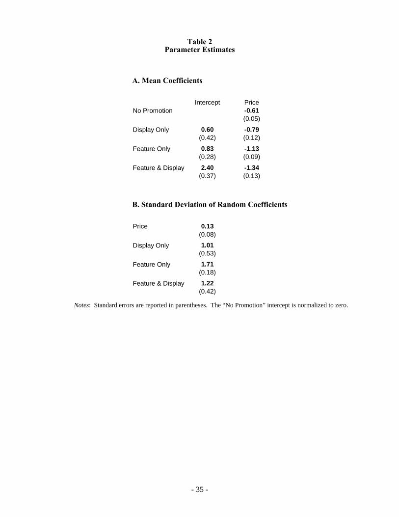
- 35 -

Table 2 Parameter Estimates

A. Mean Coefficients

Intercept PriceNo Promotion -0.61

(0.05)

Display Only 0.60 -0.79(0.42) (0.12)

Feature Only 0.83 -1.13(0.28) (0.09)

Feature & Display 2.40 -1.34(0.37) (0.13)

B. Standard Deviation of Random Coefficients

Price 0.13(0.08)

Display Only 1.01(0.53)

Feature Only 1.71(0.18)

Feature & Display 1.22(0.42)

Notes: Standard errors are reported in parentheses. The “No Promotion” intercept is normalized to zero.

- 36 -

Table 3 Elasticity Estimates

A. Own-Price Elasticities by Promotion

NoPromotion

DisplayOnly

FeatureOnly

Feature & Display

Brand A -1.62 -1.87 -1.88 -2.29(0.07) (0.24) (0.15) (0.23)

Brand B -1.66 -1.96 -1.94 -2.30(0.06) (0.24) (0.15) (0.22)

Brand C -1.56 -1.80 -1.75 -2.24(0.07) (0.22) (0.14) (0.22)

Brand D -1.80 -2.31 -2.19 -2.70(0.08) (0.28) (0.18) (0.25)

B. Elasticity Matrix

With respect to a price increase by:Brand A Brand B Brand C Brand D

Brand A -1.67 0.08 0.13 0.03(0.06) (0.01) (0.02) (0.00)

Brand B 0.20 -1.76 0.16 0.03(0.02) (0.06) (0.03) (0.01)

Brand C 0.13 0.06 -1.61 0.02(0.02) (0.01) (0.06) (0.00)

Brand D 0.16 0.07 0.14 -1.90(0.03) (0.01) (0.02) (0.07)

C. Diversion Ratios

With respect to a price increase by:Brand A Brand B Brand C Brand D

Brand A 0.00 0.11 0.08 0.09(0.00) (0.01) (0.01) (0.02)

Brand B 0.05 0.00 0.04 0.04(0.01) (0.00) (0.01) (0.01)

Brand C 0.08 0.09 0.00 0.08(0.01) (0.02) (0.00) (0.01)

Brand D 0.02 0.02 0.01 0.00(0.00) (0.00) (0.00) (0.00)

Notes: Standard errors are reported in parentheses. The cross-price elasticities and diversion ratios are calculated assuming a uniform percentage price increase across all types of promotion.

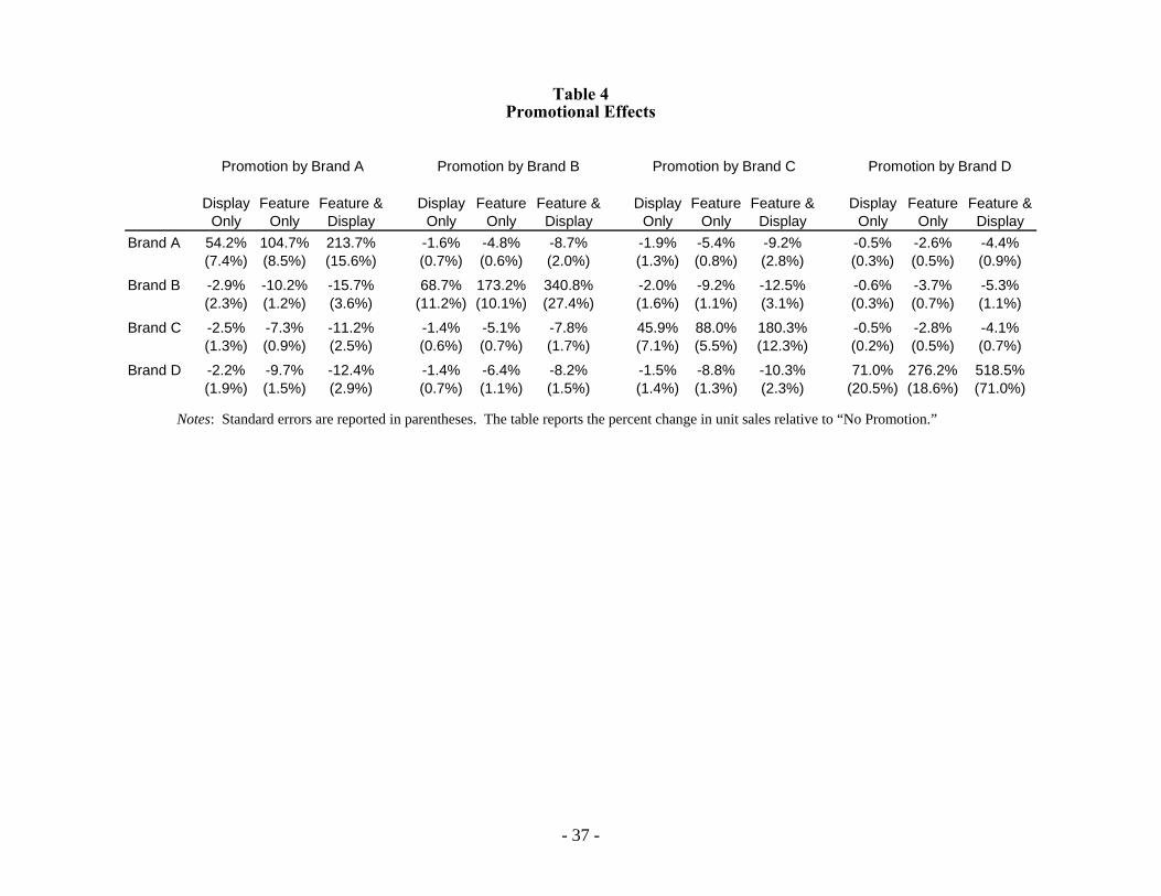
- 37 -

Table 4 Promotional Effects

Promotion by Brand A Promotion by Brand B Promotion by Brand C Promotion by Brand D

DisplayOnly

FeatureOnly

Feature &Display

DisplayOnly

FeatureOnly

Feature &Display

DisplayOnly

FeatureOnly

Feature &Display

DisplayOnly

FeatureOnly

Feature &Display

Brand A 54.2% 104.7% 213.7% -1.6% -4.8% -8.7% -1.9% -5.4% -9.2% -0.5% -2.6% -4.4%(7.4%) (8.5%) (15.6%) (0.7%) (0.6%) (2.0%) (1.3%) (0.8%) (2.8%) (0.3%) (0.5%) (0.9%)

Brand B -2.9% -10.2% -15.7% 68.7% 173.2% 340.8% -2.0% -9.2% -12.5% -0.6% -3.7% -5.3%(2.3%) (1.2%) (3.6%) (11.2%) (10.1%) (27.4%) (1.6%) (1.1%) (3.1%) (0.3%) (0.7%) (1.1%)

Brand C -2.5% -7.3% -11.2% -1.4% -5.1% -7.8% 45.9% 88.0% 180.3% -0.5% -2.8% -4.1%(1.3%) (0.9%) (2.5%) (0.6%) (0.7%) (1.7%) (7.1%) (5.5%) (12.3%) (0.2%) (0.5%) (0.7%)

Brand D -2.2% -9.7% -12.4% -1.4% -6.4% -8.2% -1.5% -8.8% -10.3% 71.0% 276.2% 518.5%(1.9%) (1.5%) (2.9%) (0.7%) (1.1%) (1.5%) (1.4%) (1.3%) (2.3%) (20.5%) (18.6%) (71.0%)

Notes: Standard errors are reported in parentheses. The table reports the percent change in unit sales relative to “No Promotion.”

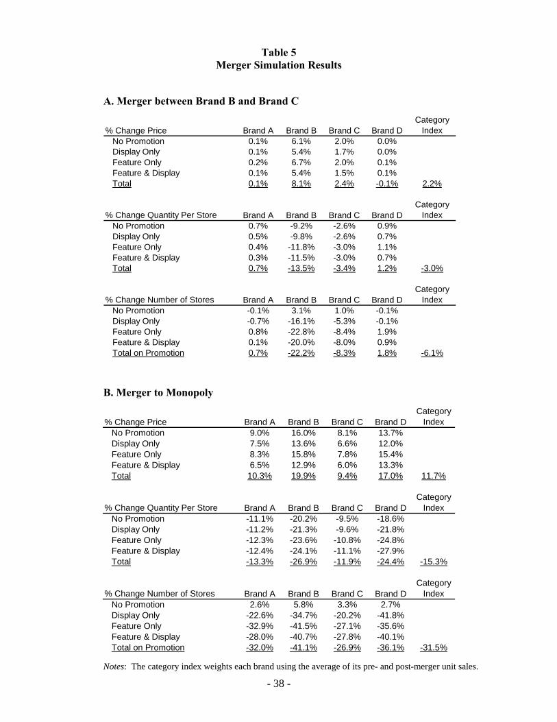
- 38 -

Table 5 Merger Simulation Results

A. Merger between Brand B and Brand C

% Change Price Brand A Brand B Brand C Brand DCategory

IndexNo Promotion 0.1% 6.1% 2.0% 0.0%Display Only 0.1% 5.4% 1.7% 0.0%Feature Only 0.2% 6.7% 2.0% 0.1%Feature & Display 0.1% 5.4% 1.5% 0.1%Total 0.1% 8.1% 2.4% -0.1% 2.2%

% Change Quantity Per Store Brand A Brand B Brand C Brand DCategory

IndexNo Promotion 0.7% -9.2% -2.6% 0.9%Display Only 0.5% -9.8% -2.6% 0.7%Feature Only 0.4% -11.8% -3.0% 1.1%Feature & Display 0.3% -11.5% -3.0% 0.7%Total 0.7% -13.5% -3.4% 1.2% -3.0%

% Change Number of Stores Brand A Brand B Brand C Brand DCategory

IndexNo Promotion -0.1% 3.1% 1.0% -0.1%Display Only -0.7% -16.1% -5.3% -0.1%Feature Only 0.8% -22.8% -8.4% 1.9%Feature & Display 0.1% -20.0% -8.0% 0.9%Total on Promotion 0.7% -22.2% -8.3% 1.8% -6.1%

B. Merger to Monopoly

% Change Price Brand A Brand B Brand C Brand DCategory

IndexNo Promotion 9.0% 16.0% 8.1% 13.7%Display Only 7.5% 13.6% 6.6% 12.0%Feature Only 8.3% 15.8% 7.8% 15.4%Feature & Display 6.5% 12.9% 6.0% 13.3%Total 10.3% 19.9% 9.4% 17.0% 11.7%

% Change Quantity Per Store Brand A Brand B Brand C Brand DCategory

IndexNo Promotion -11.1% -20.2% -9.5% -18.6%Display Only -11.2% -21.3% -9.6% -21.8%Feature Only -12.3% -23.6% -10.8% -24.8%Feature & Display -12.4% -24.1% -11.1% -27.9%Total -13.3% -26.9% -11.9% -24.4% -15.3%

% Change Number of Stores Brand A Brand B Brand C Brand DCategory

IndexNo Promotion 2.6% 5.8% 3.3% 2.7%Display Only -22.6% -34.7% -20.2% -41.8%Feature Only -32.9% -41.5% -27.1% -35.6%Feature & Display -28.0% -40.7% -27.8% -40.1%Total on Promotion -32.0% -41.1% -26.9% -36.1% -31.5%

Notes: The category index weights each brand using the average of its pre- and post-merger unit sales.

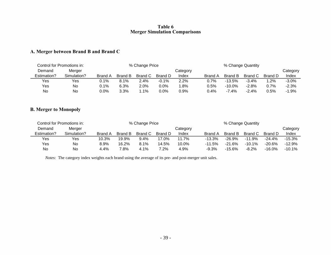
- 39 -

Table 6 Merger Simulation Comparisons

A. Merger between Brand B and Brand C

Control for Promotions in: % Change Price % Change QuantityDemand

Estimation?Merger

Simulation? Brand A Brand B Brand C Brand DCategory

Index Brand A Brand B Brand C Brand DCategory

IndexYes Yes 0.1% 8.1% 2.4% -0.1% 2.2% 0.7% -13.5% -3.4% 1.2% -3.0%Yes No 0.1% 6.3% 2.0% 0.0% 1.8% 0.5% -10.0% -2.8% 0.7% -2.3%No No 0.0% 3.3% 1.1% 0.0% 0.9% 0.4% -7.4% -2.4% 0.5% -1.9%

B. Merger to Monopoly

Control for Promotions in: % Change Price % Change QuantityDemand

Estimation?Merger

Simulation? Brand A Brand B Brand C Brand DCategory

Index Brand A Brand B Brand C Brand DCategory

IndexYes Yes 10.3% 19.9% 9.4% 17.0% 11.7% -13.3% -26.9% -11.9% -24.4% -15.3%Yes No 8.9% 16.2% 8.1% 14.5% 10.0% -11.5% -21.6% -10.1% -20.6% -12.9%No No 4.4% 7.8% 4.1% 7.2% 4.9% -9.3% -15.6% -8.2% -16.0% -10.1%

Notes: The category index weights each brand using the average of its pre- and post-merger unit sales.

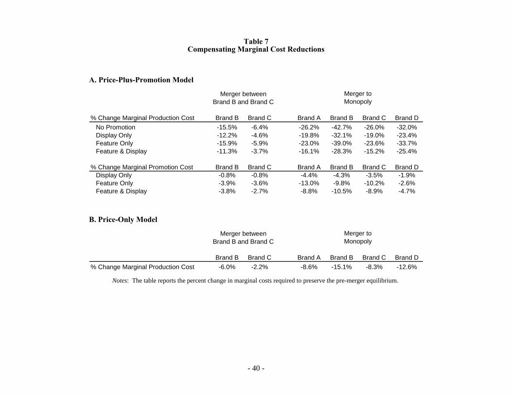
- 40 -

Table 7 Compensating Marginal Cost Reductions

A. Price-Plus-Promotion Model

Merger toMonopoly

% Change Marginal Production Cost Brand B Brand C Brand A Brand B Brand C Brand DNo Promotion -15.5% -6.4% -26.2% -42.7% -26.0% -32.0%Display Only -12.2% -4.6% -19.8% -32.1% -19.0% -23.4%Feature Only -15.9% -5.9% -23.0% -39.0% -23.6% -33.7%Feature & Display -11.3% -3.7% -16.1% -28.3% -15.2% -25.4%

% Change Marginal Promotion Cost Brand B Brand C Brand A Brand B Brand C Brand DDisplay Only -0.8% -0.8% -4.4% -4.3% -3.5% -1.9%Feature Only -3.9% -3.6% -13.0% -9.8% -10.2% -2.6%Feature & Display -3.8% -2.7% -8.8% -10.5% -8.9% -4.7%

Merger between Brand B and Brand C

B. Price-Only Model

Merger toMonopoly

Brand B Brand C Brand A Brand B Brand C Brand D% Change Marginal Production Cost -6.0% -2.2% -8.6% -15.1% -8.3% -12.6%

Merger between Brand B and Brand C

Notes: The table reports the percent change in marginal costs required to preserve the pre-merger equilibrium.

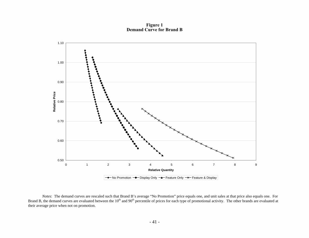
- 41 -

Figure 1 Demand Curve for Brand B

0.50

0.60

0.70

0.80

0.90

1.00

1.10

0 1 2 3 4 5 6 7 8 9

Relative Quantity

Rel

ativ

e Pr

ice

No Promotion Display Only Feature Only Feature & Display

Notes: The demand curves are rescaled such that Brand B’s average “No Promotion” price equals one, and unit sales at that price also equals one. For Brand B, the demand curves are evaluated between the 10th and 90th percentile of prices for each type of promotional activity. The other brands are evaluated at their average price when not on promotion.

Documents

Mergers when Firms Compete by Choosing both Price and Promotion