Medical Image Analysis (Dhawan/Medical Image Analysis 2E) || Introduction

CHAPTER 1

INTRODUCTION

The last two decades have witnessed signifi cant advances in medical imaging and computerized medical image processing. These advances have led to new two - , three - , and multidimensional imaging modalities that have become important clinical tools in diagnostic radiology. The clinical signifi cance of radiological imaging modal-ities in diagnosis and treatment of diseases is overwhelming. While planar X - ray imaging was the only radiological imaging method in the early part of the last century, several modern imaging modalities are in practice today to acquire anatomical, physi-ological, metabolic, and functional information from the human body. Commonly used medical imaging modalities capable of producing multidimensional images for radiological applications are X - ray computed tomography (X - ray CT), magnetic resonance imaging (MRI), single photon emission computed tomography (SPECT), positron emission tomography (PET), and ultrasound. It should be noted that these modern imaging methods involve sophisticated instrumentation and equipment using high - speed electronics and computers for data collection and image reconstruction and display. Simple planar radiographic imaging methods such as chest X rays and mammograms usually provide images on a fi lm that is exposed during imaging through an external radiation source (X ray) and then developed to show images of body organs. These planar radiographic imaging methods provide high - quality analog images that are shadows or two - dimensional (2 - D) projected images of three - dimensional (3 - D) organs. Recent complex medical imaging modalities such as X - ray CT, MRI, SPECT, PET, and ultrasound heavily utilize computer technology for creation and display of digital images. Using the computer, multidimensional digital images of physiological structures can be processed and manipulated to visualize hidden characteristic diagnostic features that are diffi cult or impossible to see with planar imaging methods. Further, these features of interest can be quantifi ed and analyzed using sophisticated computer programs and models to understand their behavior to help with a diagnosis or to evaluate treatment protocols. Nevertheless, the clinical signifi cance of simple planar imaging methods such as X - ray radiographs (e.g., chest X ray and mammograms) must not be underestimated as they offer cost - effective and reliable screening tools that often provide important diagnostic informa-tion suffi cient to make correct diagnosis and judgment about the treatment.

However, in many critical radiological applications, the multidimensional visualization and quantitative analysis of physiological structures provide un-precedented clinical information extremely valuable for diagnosis and treatment.

Medical Image Analysis, Second Edition, by Atam P. DhawanCopyright © 2011 by the Institute of Electrical and Electronics Engineers, Inc.

1

c01.indd 1c01.indd 1 11/17/2010 1:40:38 PM11/17/2010 1:40:38 PM

2 CHAPTER 1 INTRODUCTION

Computerized processing and analysis of medical imaging modalities provides a powerful tool to help physicians. Thus, computer programs and methods to process and manipulate the raw data from medical imaging scanners must be carefully developed to preserve and enhance the real clinical information of interest rather than introducing additional artifacts. The ability to improve diagnostic information from medical images can be further enhanced by designing computer processing algorithms intelligently. Often, incorporating relevant knowledge about the physics of imaging, instrumentation, and human physiology in computer programs pro-vides outstanding improvement in image quality as well as analysis to help inter-pretation. For example, incorporating knowledge about the geometrical location of the source, detector, and patient can reduce the geometric artifacts in the recon-structed images. Further, the use of geometrical locations and characteristic signa-tures in computer - aided enhancement, identifi cation, segmentation, and analysis of physiological structures of interest often improves the clinical interpretation of medical images.

1.1. MEDICAL IMAGING: A COLLABORATIVE PARADIGM

As discussed above, with the advent and enhancement of modern medical imaging modalities, intelligent processing of multidimensional images has become crucial in conventional or computer - aided interpretation for radiological and diagnostic applications. Medical imaging and processing in diagnostic radiology has evolved with signifi cant contributions from a number of disciplines including mathematics, physics, chemistry, engineering, and medicine. This is evident when one sees a medical imaging scanner such as an MRI or PET scanner. The complexity of instru-mentation and computer - aided data collection and image reconstruction methods clearly indicates the importance of system integration as well as a critical understand-ing of the physics of imaging and image formation. Intelligent interpretation of medical images requires understanding the interaction of the basic unit of imaging (such as protons in MRI, or X - ray photons in X - ray CT) in a biological environment, formation of a quantifi able signal representing the biological information, detection and acquisition of the signal of interest, and appropriate image reconstruction. In brief, intelligent interpretation and analysis of biomedical images require an understanding of the acquisition of images.

A number of computer vision methods have been developed for a variety of applications in image processing, segmentation, analysis, and recognition. However, medical image reconstruction and processing requires specialized knowledge of the specifi c medical imaging modality that is used to acquire images. The character of the collected data in the application environment (such as imaging the heart through MRI) should be properly understood for selecting or developing useful methods for intelligent image processing, analysis, and interpretation. The use of application domain knowledge can be useful in selecting or developing the most appropriate image reconstruction and processing methods for accurate analysis and interpretation.

c01.indd 2c01.indd 2 11/17/2010 1:40:38 PM11/17/2010 1:40:38 PM

1.2. MEDICAL IMAGING MODALITIES 3

1.2. MEDICAL IMAGING MODALITIES

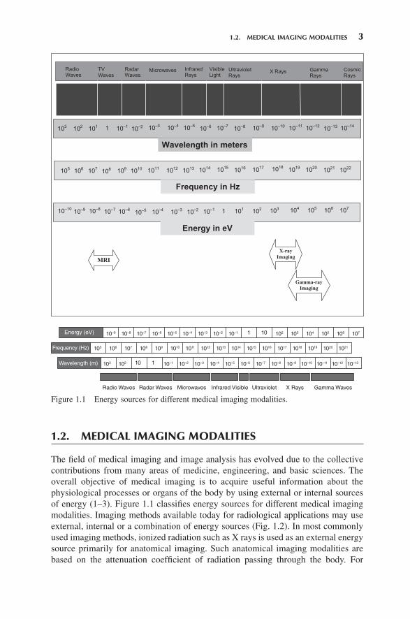
The fi eld of medical imaging and image analysis has evolved due to the collective contributions from many areas of medicine, engineering, and basic sciences. The overall objective of medical imaging is to acquire useful information about the physiological processes or organs of the body by using external or internal sources of energy (1 – 3) . Figure 1.1 classifi es energy sources for different medical imaging modalities. Imaging methods available today for radiological applications may use external, internal or a combination of energy sources (Fig. 1.2 ). In most commonly used imaging methods, ionized radiation such as X rays is used as an external energy source primarily for anatomical imaging. Such anatomical imaging modalities are based on the attenuation coeffi cient of radiation passing through the body. For

Figure 1.1 Energy sources for different medical imaging modalities.

10–10

Radio Waves

TV Waves

Radar Waves

Microwaves Infrared Rays

Visible Light

Ultraviolet Rays

X Rays Gamma Rays

102 101 1 10–1 10–2 10–3 10–410–6 10–7 10–8

Wavelength in meters

Frequency in Hz

10–5 10–9 10–10 10–11 10–12 10–13 10–14103

106 107 109 1010 1011 1012 1014 1015 10161013 1017 1018 1019 1020 1021 1022105 108

Energy in eV

10–9 10–8 10–610–5 10–4 10–3 10–1 1 101

10–2 102 103 104 105 106 10710–7

MRI

X-ray Imaging

Gamma-ray Imaging

Cosmic Rays

Energy (eV)

Frequency (Hz)

Wavelength (m)

10–9 10–8 10–7 10–6 10–5 10–4 10–3

103 102 10 1 10–1 10–2 10–3 10–4 10–5 10–6 10–7 10–8 10–9 10–10 10–11 10–12 10–13

10–2 10–1 1 10 102 103 104 105

105 106 107 108 109 1010 1011 1012 1013 1014 1015 1016 1017 1018 1019 1020 1021

106 107

Radio Waves Radar Waves Microwaves Infrared Visible Ultraviolet X Rays Gamma Waves

c01.indd 3c01.indd 3 11/17/2010 1:40:38 PM11/17/2010 1:40:38 PM


example, X - ray radiographs and X - ray CT imaging modalities measure attenuation coeffi cients of X ray that are based on the density of the tissue or part of the body being imaged. The images of chest radiographs show a spatial distribution of X - ray attenuation coeffi cients refl ecting the overall density variations of the anatomical parts in the chest. Another example of external energy source - based imaging is ultrasound or acoustic imaging. Nuclear medicine imaging modalities use an internal energy source through an emission process to image the human body. For emission imaging, radioactive pharmaceuticals are injected into the body to interact with selected body matter or tissue to form an internal source of radioactive energy that is used for imaging. The emission imaging principle is applied in SPECT and PET. Such types of nuclear medicine imaging modalities provide useful metabolic

Figure 1.2 A classifi cation of different medical imaging modalities with respect to the type of energy source used for imaging.

Source of EnergyUsed for Imaging

ExternalInternal

Combination: External and Internal

Nuclear Medicine:Single PhotonEmission Tomography(SPECT)

Nuclear Medicine:Positron EmissionTomography(PET)

Magnetic ResonanceImaging: MRI, PMRI,FMRI

Optical FluorescenceImaging

Electrical ImpedanceImaging

MedicalImaging

Modalities

X-Ray Radiographs

X-Ray Mammography

X-Ray Computed Tomography

Optical Transmission and Transillumination Imaging

Ultrasound Imaging and Tomography

c01.indd 4c01.indd 4 11/17/2010 1:40:38 PM11/17/2010 1:40:38 PM

1.2. MEDICAL IMAGING MODALITIES 5

information about the physiological functions of the organs. Further, a clever com-bination of external stimulation on internal energy sources can be used in medical imaging to acquire more accurate information about the tissue material and physi-ological responses and functions. MRI uses external magnetic energy to stimulate selected atomic nuclei such as hydrogen protons. The excited nuclei become the internal source of energy to provide electromagnetic signals for imaging through the process of relaxation. MRI of the human body provides high - resolution images of the human body with excellent soft - tissue characterization capabilities. Recent advances in MRI have led to perfusion and functional imaging aspects of human tissue and organs (3 – 6) . Another emerging biophysiological imaging modality is fl uorescence imaging, which uses an external ultraviolet energy source to stimulate the internal biological molecules of interest, which absorb the ultraviolet energy, become internal sources of energy, and then emit the energy at visible electromag-netic radiation wavelengths (7) .

Before a type of energy source or imaging modality is selected, it is important to understand the nature of physiological information needed for image formation. In other words, some basic questions about the information of interest should be answered. What information about the human body is needed? Is it anatomical, physiological, or functional? What range of spatial resolution is acceptable? The selection of a specifi c medical imaging modality often depends on the type of sus-pected disease or localization needed for proper radiological diagnosis. For example, some neurological disorders and diseases demand very high resolution brain images for accurate diagnosis and treatment. On the other hand, full - body SPECT imaging to study metastasizing cancer does not require submillimeter imaging resolution. The information of interest here is cancer metastasis in the tissue, which can be best obtained from the blood fl ow in the tissue or its metabolism. Breast imaging can be performed using X rays, magnetic resonance, nuclear medicine, or ultrasound. But the most effective and economical breast imaging modality so far has been X - ray mammography because of its simplicity, portability, and low cost. One important source of radiological information for breast imaging is the presence and distribution of microcalcifi cations in the breast. This anatomical information can be obtained with high resolution using X rays.

There is no perfect imaging modality for all radiological applications and needs. In addition, each medical imaging modality is limited by the corresponding physics of energy interactions with human body (or cells), instrumentation, and often physiological constraints. These factors severely affect the quality and resolution of images, sometimes making the interpretation and diagnosis diffi cult. The perfor-mance of an imaging modality for a specifi c test or application is characterized by sensitivity and specifi city factors. Sensitivity of a medical imaging test is defi ned primarily by its ability to detect true information. Let us suppose we have an X - ray imaging scanner for mammography. The sensitivity for imaging microcalcifi cations for a mammography scanner depends on many factors including the X - ray wave-length used in the beam, intensity, and polychromatic distribution of the input radia-tion beam, behavior of X rays in breast tissue such as absorption and scattering coeffi cients, and fi lm/detector effi ciency to collect the output radiation. These factors eventually affect the overall signal - to - noise ratio leading to the loss of sensitivity of

c01.indd 5c01.indd 5 11/17/2010 1:40:39 PM11/17/2010 1:40:39 PM


detecting microcalcifi cations. The specifi city for a test depends on its ability to not detect information when it is truly not there.

1.3. MEDICAL IMAGING: FROM PHYSIOLOGY TO INFORMATION PROCESSING

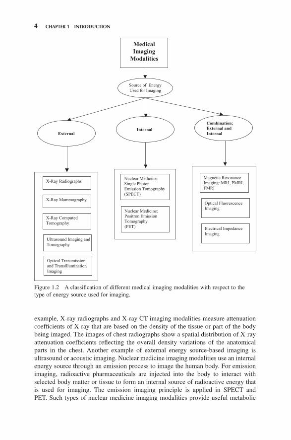
From physiology to image interpretation and information retrieval, medical imaging may be defi ned as a fi ve - step paradigm (see Fig. 1.3 ). The fi ve - step paradigm allows acquisition and analysis of useful information to understand the behavior of an organ or a physiological process.

1.3.1 Understanding Physiology and Imaging Medium

The imaged objects (organs, tissues, and specifi c pathologies) and associated physi-ological properties that could be used for obtaining signals suitable for the formation of an image must be studied for the selection of imaging instrumentation. This information is useful in designing image processing and analysis techniques for correct interpretation. Information about the imaging medium may involve static or dynamic properties of the biological tissue. For example, tissue density is a static property that causes attenuation of an external radiation beam in X - ray imaging modality. Blood fl ow, perfusion, and cardiac motion are examples of dynamic physi-ological properties that may alter the image of a biological entity. Consideration of the dynamic behavior of the imaging medium is essential in designing compensation methods needed for correct image reconstruction and analysis. Motion artifacts pose serious limitations on data collection time and resolution in medical imaging instru-mentation and therefore have a direct effect on the development of image processing methods.

Figure 1.3 A collaborative multidisciplinary paradigm of medical imaging research and applications .

Physics of ImagingPhysiology

andKnowledge Base

ImagingInstrumentation

Image Analysis, Modeling, and

Application

Data Acquisition andImage Reconstruction

c01.indd 6c01.indd 6 11/17/2010 1:40:39 PM11/17/2010 1:40:39 PM

1.3. MEDICAL IMAGING: FROM PHYSIOLOGY TO INFORMATION PROCESSING 7

1.3.2 Physics of Imaging

The next important consideration is the principle of imaging to be used for obtaining the data. For example, X - ray imaging modality uses transmission of X rays through the body as the basis of imaging. On the other hand, in the nuclear medicine modal-ity, SPECT uses the emission of gamma rays resulting from the interaction of a radiopharmaceutical substance with the target tissue. The emission process and the energy range of gamma rays cause limitations on the resolution and data acquisition time for imaging. The associated methods for image formation in transmission and emission imaging modalities are so different that it is diffi cult to see the same level of anatomical information from both modalities. SPECT and PET provide images that are poor in contrast and anatomical details, while X - ray CT provides sharper images with high - resolution anatomical details. MRI provides high - resolution ana-tomical details with excellent soft - tissue contrast (6, 7) .

1.3.3 Imaging Instrumentation

The instrumentation used in collecting the data is one of the most important factors defi ning the image quality in terms of signal - to - noise ratio, resolution, and ability to show diagnostic information. Source specifi cations of the instrumentation directly affect imaging capabilities. In addition, detector responses such as nonlinearity, low effi ciency, long decay time, and poor scatter rejection may cause artifacts in the image. An intelligent image formation and processing technique should be the one that provides accurate and robust detection of features of interest without any arti-facts to help diagnostic interpretation.

1.3.4 Data Acquisition and Image Reconstruction

The data acquisition methods used in imaging play an important role in image for-mation. Optimized with the imaging instrumentation, the data collection methods become a decisive factor in determining the best temporal and spatial resolution. It is also crucial in developing strategies to reduce image artifacts through active fi lter-ing or postprocessing methods. For example, in X - ray CT, the spatially distributed signal is based on the number of X - ray photons reaching the detector within a time interval. The data for 3 - D imaging may be obtained using a parallel - , cone - , or spiral - beam scanning method. Each of these scanning methods causes certain con-straints on the geometrical reconstruction of the object under imaging. Since the scanning time in each method may be different, spatial resolution has to be balanced by temporal resolution. This means that a faster scan would result in an image with a lower spatial resolution. On the other hand, a higher spatial resolution method would normally require longer imaging time. In dynamic studies where information about blood fl ow or a specifi c functional activity needs to be acquired, the higher resolution requirement is usually compromised. Image reconstruction algorithms such as backprojection, iterative, and Fourier transform methods are tailored to incorporate specifi c information about the data collection methods and scanning geometry. Since the image quality may be affected by the data collection methods,

c01.indd 7c01.indd 7 11/17/2010 1:40:39 PM11/17/2010 1:40:39 PM


the image reconstruction and processing methods should be designed to optimize the representation of diagnostic information in the image.

1.3.5 Image Analysis and Applications

Image processing and analysis methods are aimed at the enhancement of diagnostic information to improve manual or computer - assisted interpretation of medical images. Often, certain transformation methods improve the visibility and quantifi ca-tion of features of interest. Interactive and computer - assisted intelligent medical image analysis methods can provide effective tools to help the quantitative and qualitative interpretation of medical images for differential diagnosis, intervention, and treatment monitoring. Intelligent image processing and analysis tools can also help in understanding physiological processes associated with the disease and its response to a treatment.

1.4. GENERAL PERFORMANCE MEASURES

Let us defi ne some measures often used in the evaluation of a medical imaging or diagnostic test for detecting an object such as microcalcifi cations or a physiological condition such as cancer. A “ positive ” observation in an image means that the object was observed in the test. A “ negative ” observation means that the object was not observed in the test. A “ true condition ” is the actual truth, while an observation is the outcome of the test. Four basic measures are defi ned from the set of true condi-tions and observed information as shown in Figure 1.4 . These basic measures are true positive, false positive, false negative, and true negative rates or fractions. For example, an X - ray mammographic image should show only the regions of pixels with bright intensity (observed information) corresponding to the microcalcifi cation areas (true condition when the object is present). Also, the mammographic image should not show similar regions of pixels with bright intensity corresponding to the

Figure 1.4 A conditional matrix for defi ning four basic performance measures of receiver operating characteristic curve (ROC) analysis.

True Positive

True Negative

False Negative

False Positive

True Condition

Object is present.

Object is NOT present.

Object is observed.

Object is NOT observed.

ObservedInformation

c01.indd 8c01.indd 8 11/17/2010 1:40:39 PM11/17/2010 1:40:39 PM

1.4. GENERAL PERFORMANCE MEASURES 9

areas where there is actually no microcalcifi cation (true condition when the object is not present).

Let us assume the total number of examination cases to be N tot , out of which N tp cases have positive true condition with the actual presence of the object and the remaining cases, N tn , have negative true condition with no object present. Let us suppose these cases are examined via the test for which we need to evaluate accu-racy, sensitivity, and specifi city factors. Considering the observer does not cause any loss of information or misinterpretation, let N otp (true positive) be the number of positive observations from N tp positive true condition cases and N ofn (false nega-tive) be the number of negative observations from N tp positive true condition cases. Also, let N otn (true negative) be the number of negative observations from N tn nega-tive true condition cases and N ofp (false positive) be the number of positive observa-tions from N tn negative true condition cases.

Thus,

N N N N N Ntp otp ofn tn ofp otn= + = +and .

1. True positive fraction (TPF) is the ratio of the number of positive observations to the number of positive true condition cases.

TPF /= N Notp tp . (1.1)

2. False negative fraction (FNF) is the ratio of the number of negative observa-tions to the number of positive true condition cases.

FNF /= N Nofn tp (1.2)

3. False positive fraction (FPF) is the ratio of the number of positive observations to the number of negative true condition cases.

FPF /= N Nofp tn (1.3)

4. True negative fraction (TNF) is the ratio of the number of negative observa-tions to the number of negative true condition cases.

TNF /= N Notn tn (1.4)

It should be noted that

TPF FNF

TNF FPF

+ =+ =

1

1. (1.5)

A graph between TPF and FPF is called a receiver operating characteristic (ROC) curve for a specifi c medical imaging or diagnostic test for detection of an object. Various points on the ROC curves shown in Figure 1.5 indicate different decision thresholds used for classifi cation of the examination cases into positive and negative observations, and therefore defi ning specifi c sets of paired values of TPF and FPF. It should also be noted that statistical random trials with equal probability of positive and negative observations would lead to the diagonally placed straight line as the ROC curve. Different tests and different observers may lead to different ROC curves for the same object detection.

c01.indd 9c01.indd 9 11/17/2010 1:40:40 PM11/17/2010 1:40:40 PM


True positive fraction is also called the sensitivity while the true negative fraction is known as specifi city of the test for detection of an object. Accuracy of the test is given by a ratio of correct observation to the total number of examination cases. Thus,

Accuracy ( )//= +N N Notp otn tot . (1.6)

The positive predictive value (PPV) considered to be the same as precision of a diagnostic test is measured as

PPV /= +N N Notp otp ofp( ). (1.7)

In other words, different imaging modalities and observers may lead to different accuracy, PPV, sensitivity, and specifi city levels.

The accuracy, sensitivity, and specifi city factors are given serious consider-ation when selecting a modality for radiological applications. For example, X - ray mammography is so successful in breast imaging because it provides excellent sensitivity and specifi city for imaging breast calcifi cations. In neurological applica-tions requiring a demanding soft - tissue contrast, however, MRI provides better sensitivity and specifi city factors than X - ray imaging.

1.4.1 An Example of Performance Measure

Let us assume that 100 female patients were examined with X - ray mammography. The images were observed by a physician to classify into one of the two classes: normal and cancer. The objective here is to determine the basic performance mea-sures of X - ray mammography for detection of breast cancer. Let us assume that all patients were also tested through tissue - biopsy examination to determine the true condition. If the result of the biopsy examination is positive, the cancer (object) is present as the true condition. If the biopsy examination is negative, the cancer (object) is not present as the true condition. If the physician diagnoses the cancer from X - ray mammography, the object (cancer) is observed. Let us assume the fol-lowing distribution of patients with respect to the true conditions and observed information:

Figure 1.5 ROC curves, with “ a ” indicating better classifi cation ability than “ b, ” and “ c ” showing the random probability.

FPF

TPF

b

a

c

c01.indd 10c01.indd 10 11/17/2010 1:40:40 PM11/17/2010 1:40:40 PM

1.5. BIOMEDICAL IMAGE PROCESSING AND ANALYSIS 11

1. Total number of patients = N tot = 100

2. Total number of patients with biopsy - proven cancer (true condition of object present) = N tp = 10

3. Total number of patients with biopsy - proven normal tissue (true condition of object NOT present) = N tn = 90

4. Of the patients with cancer N tp , the number of patients diagnosed by the physi-cian as having cancer = number of true positive cases = N otp = 8

5. Of the patients with cancer N tp , the number of patients diagnosed by the physi-cian as normal = number of false negative cases = N ofn = 2

6. Of the normal patients N tn , the number of patients rated by the physician as normal = number of true negative cases = N otn = 85

7. Of the normal patients N tn , the number of patients rated by the physician as having cancer = number of false positive cases = N ofp = 5

Now the TPF, FNF, FPF, and TNF can be computed as

TPF /= =8 10 0 8.

FNF /= =2 10 0 2.

FPF /= =5 90 0 0556.

TNF /= =85 90 0 9444.

This should be noted that the above values satisfy Equation 1.5 as

TPF FNF and FPF TNF+ = + =1 0 1 0. .

1.5. BIOMEDICAL IMAGE PROCESSING AND ANALYSIS

A general - purpose biomedical image processing and image analysis system must have three basic components: an image acquisition system, a digital computer, and an image display environment. Figure 1.6 shows a schematic block diagram of a biomedical image processing and analysis system.

The image acquisition system usually converts a biomedical signal or radia-tion carrying the information of interest to a digital image. A digital image is

Figure 1.6 A general schematic diagram of biomedical image analysis system.

c01.indd 11c01.indd 11 11/17/2010 1:40:40 PM11/17/2010 1:40:40 PM


represented by an array of digital numbers that can be read by the processing com-puter and displayed as a two - , three, or multidimensional image. As introduced above, medical imaging modalities use different image acquisition systems as a part of the imaging instrumentation. The design of the image acquisition system depends on the type of modality and detector requirements. In some applications, the output of the scanner may be in analog form, such as a fi lm - mammogram or a chest X - ray radiograph. In such applications, the image acquisition system may include a suitable light source to illuminate the radiograph (the fi lm) and a digitizing camera to convert the analog image into a digital picture. Other means of digitizing an image include several types of microdensitometers and laser scanners. There is a variety of sources of biomedical imaging applications. The data acquisition system has to be modifi ed accordingly. For example, a microscope can be directly hooked up with a digitizing camera for acquisition of images of a biopsy sample on a glass slide. But such a digitizing camera is not needed for obtaining images from an X - ray CT scanner. Thus, the image acquisition system differs across applications.

The second part of the biomedical image processing and analysis system is a computer used to store digital images for further processing. A general - purpose computer or a dedicated array processor can be used for image analysis. The dedi-cated hardwired image processors may be used for the real - time image processing operations such as image enhancement, pseudo - color enhancement, mapping, and histogram analysis.

A third essential part of the biomedical image processing and analysis system is the image display environment where the output image can be viewed after the required processing. Depending on the application, there may be a large variation in the requirements of image display environment in terms of resolution grid size, number of gray levels, number of colors, split - screen access, and so on. There might be other output devices such as a hard - copy output machine or printer that can also be used in conjunction with the regular output display monitor.

For an advanced biomedical image analysis system, the image display environ-ment may also include a real - time image processing unit that may have some built - in processing functions for quick manipulation. The central image processing unit, in such systems, does the more complicated image processing and analysis only. For example, for radiological applications, the image display unit should have a fast and fl exible environment to manipulate the area of interest in the image. This manipula-tion may include gray - level remapping, pseudo - color enhancement, zoom - in, or split - screen capabilities to aid the attending physician in seeing more diagnostic information right away. This type of real - time image processing may be part of the image - display environment in a modern sophisticated image analysis system that is designed for handling the image analysis and interpretation tasks for biomedical applications (and many others). The display environment in such systems includes one or more pixel processors or point processors (small processing units or single - board computers) along with a number of memory planes, which act as buffers. These buffers or memory planes provide an effi cient means of implementing a number of look - up - tables (LUTs) without losing the original image data. The spe-cialized hardwired processing units including dedicated processors are accessed and

c01.indd 12c01.indd 12 11/17/2010 1:40:40 PM11/17/2010 1:40:40 PM

1.5. BIOMEDICAL IMAGE PROCESSING AND ANALYSIS 13

communicated with by using the peripheral devices such as keyboard, data tablet, mouse, printer, and high - resolution monitors.

There are several image processing systems available today that satisfy the usual requirements (as discussed above) of an effi cient and useful biomedical image analysis system. All these systems are based on a special pipeline architecture with an external host computer and/or an array processor allowing parallel processing and effi cient communication among various dedicated processors for real - time or near real - time split - screen image manipulation and processing performance. Special - purpose image processing architectures includes array processors, graphic accelera-tors, logic processors, and fi eld programmable gate arrays (FPGA).

As discussed above, every imaging modality has limitations that affect the accuracy, sensitivity, and specifi city factors, which are extremely important in diag-nostic radiology. Scanners are usually equipped with instrumentation to provide external radiation or energy source (as needed) and measure an output signal from the body. The output signal may be attenuated radiation or another from of energy carrying information about the body. The output signal is eventually transformed into an image to represent the information about the body. For example, an X - ray mammography scanner uses an X - ray tube to generate a radiation beam that passes through the breast tissue. As a result of the interactions among X - ray photons and breast tissue, the X - ray beam is attenuated. The attenuated beam of X - ray radiation coming out of the breast is then collected on a radiographic fi lm. The raw signals obtained from instrumentation of an imaging device or scanner are usually prepro-cessed for a suitable transformation to form an image that makes sense from the physiological point of view and is easy to interpret. Every imaging modality uses some kind of image reconstruction method to provide the fi rst part of this transfor-mation for conversions of raw signals into useful images. Even after a good recon-struction or initial transformation, images may not provide useful information with a required localization to help interpretation. This is particularly important when the information about suspect objects is occluded or overshadowed by other parts of the body. Often reconstructed images from scanners are degraded in a way that unless the contrast and brightness are adjusted, the objects of interest may not be easily visualized. Thus, an effective and effi cient image processing environment is a vital part of the medical imaging system.

Since the information of interest about biological objects often is associated with characteristic features, it is crucial to use specially designed image processing methods for visualization and analysis of medical images. It is also important to know about the acquisition and transformation methods used for reconstruction of images before appropriate image processing and analysis algorithms are designed and applied. With the new advances in image processing, adaptive learning, and knowledge - based intelligent analysis, the specifi c needs of medical image analysis to improve diagnostic information for computer - aided diagnosis can be addressed.

Figure 1.7 a,b shows an example of feature - adaptive contrast enhancement processing as applied to a part of the mammogram to enhance microcalcifi cation areas. Figure 1.7 c shows the result of a standard histogram equalization method commonly used for contrast enhancement in image processing. It is clear that stan-dard image processing algorithms may not be helpful in medical image processing.

c01.indd 13c01.indd 13 11/17/2010 1:40:40 PM11/17/2010 1:40:40 PM


Specifi c image processing operations are needed to deal with the information of radiological interest. The following chapters will introduce fundamental principles of medical imaging systems and image processing tools. The latter part of the book is dedicated to the design and application of intelligent and customized image pro-cessing algorithms for radiological image analysis.

1.6. MATLAB IMAGE PROCESSING TOOLBOX

The MATLAB image processing toolbox is a compilation of a number of useful commands and subroutines for effi cient image processing operations. The image processing toolbox provides extensive information with syntax and examples about each command. It is strongly recommended that readers go through the description of commands in the help menu and follow tutorials for various image processing tasks. Some of the introductory commands are described below.

1.6.1 Digital Image Representation

A 2 - D digital image of spatial size M × N pixels (picture elements with M rows and N columns) may be represented by a function f ( x , y ) where ( x , y ) is the location of

Figure 1.7 (a) a digital mammogram image; (b) microcalcifi cation enhanced image through feature adaptive contrast enhancement algorithm; and (c) enhanced image through histogram equalization method (see Chapter 9 for details on image enhancement algorithms).

(a) (b) (c)

c01.indd 14c01.indd 14 11/17/2010 1:40:40 PM11/17/2010 1:40:40 PM

1.6. MATLAB IMAGE PROCESSING TOOLBOX 15

a pixel whose gray level value (or brightness) is given by the function f ( x , y ) with x = 1, 2, … , M ; y = 1, 2, … , N . The brightness values or gray levels of the function f ( x , y ) are digitized in a specifi c resolution such as 8 - bit (256 levels), 12 - bit (4096 levels), or more. For computer processing, a digital image can be described by a 2 - D matrix [F] of elements whose values and locations represents, respectively, the gray levels and location of pixels in the image as

F =

f f f N

f f f N

f M f M f M N

( , ) ( , ) . . ( , )

( , ) ( , ) ( , )

( , ) ( , ) ( , )

1 1 1 2 1

2 1 2 2 2

1 2

⎡⎡

⎣

⎢⎢⎢⎢⎢⎢

⎤

⎦

⎥⎥⎥⎥⎥⎥

. (1.8)

For example, a synthetic image of size 5 × 5 pixels with “ L ” letter shape of gray level 255 over a background of gray level 20 may be represented as

F =

20 20 255 20 20

20 20 255 20 20

20 20 255 20 20

20 20 255 20 20

20 20 255 255 2555

⎡

⎣

⎢⎢⎢⎢⎢⎢

⎤

⎦

⎥⎥⎥⎥⎥⎥

. (1.9)

It is clear from the above that a digital image is discrete in both space and gray - level values as pixels are distributed over space locations. Thus, any static image is char-acterized by (1) spatial resolution (number of pixels in x - and y - directions such as 1024 × 1024 pixels for 1M pixel image), and (2) gray - level resolution (number of brightness levels such as 256 in 8 - bit resolution image). In addition, images can also be characterized by number of dimensions (2 - D, 3 - D, etc.) and temporal resolution if images are taken as a sequence with regular time interval. A 4 - D image data set may include, for example, 3 - D images taken with a temporal resolution of 0.1 s.

Images that are underexposed (and look darker) may not utilize the entire gray - level range. For example, an underexposed image with 8 - bit gray - level resolu-tion (0 – 255 gray - level range) may have gray - level values from 0 to 126. Thus, the maximum brightness level in the image appears to be at about half the intensity it could have been if it was stretched to 255. One solution to this problem is to stretch the gray - level range from 0 – 126 to 0 – 255 linearly. Such a method is commonly known as gray - level scaling or stretching and can be shown as a linear mapping as

g x yd c

b af x y a c( , )

( )

( )( ( , ) )= −

−− + (1.10)

where an original image f ( x , y ) with gray - level range ( a , b ) is scaled linearly to an output image g ( x , y ) with gray - level range ( c , d ).

Sometimes an image shows some pixels at the maximum brightness intensity level, yet the rest of the image appears to be quite dark. This may happen if there are some very high values in the image but most of other pixels have very low values. For example, a Fourier transform of an image may have a very high dc value

c01.indd 15c01.indd 15 11/17/2010 1:40:41 PM11/17/2010 1:40:41 PM


but other parts of the frequency spectrum carry very low values. In such cases, a nonlinear transformation is used to reduce the wide gap between the low and high values. A commonly used logarithm transformation for displaying images with a wide range of values is expressed as log{abs( f )} or log{1 + abs( f )} such that

g x y f x y( , ) log( ( , ) )=

or

g x y f x y( , ) log( ( , ) )= +1 (1.11)

Examples of image scaling and log - transformation operations in the MATLAB image processing toolbox are shown in Figures 1.8 and 1.9 . More image processing operations are described in Chapter 9 .

1.6.2 Basic MATLAB Image Toolbox Commands

In the MATLAB environment, an image can be read and displayed using the image processing toolbox as

>> f = imread( ‘ fi lename.format ’ );

Figure 1.8 An original mammogram image (left) and the gray - level scaled image (right).

Original Enhanced

Figure 1.9 M - Script code for the example shown in Figure 1.8 .

x = imread(f);x = rgb2gray(x);figure('Name', 'Contrast Enhancement');subplot(1,2,1) imshow(x);title('Original');subplot(1,2,2) imshow(x, []);title('Enhanced');

c01.indd 16c01.indd 16 11/17/2010 1:40:41 PM11/17/2010 1:40:41 PM

1.6. MATLAB IMAGE PROCESSING TOOLBOX 17

There are several image storage and compression formats in which the image data is stored and managed. Some of the common formats are JPEG (created by Joint Photography Expert Group), graphical interchange format (GIF), tagged image fi le format (TIFF); and Windows Bitmap (BMP).

The format could be any of the above allowed formats. The semicolon (;) is added if the program is continued, otherwise the MATLAB displays the results of the operation(s) given in the preceding command. Directory information can be added in the command before the fi lename such as

>> f = imread( ‘ C:\medimages\mribrain1.jpg ’ );

The size information is automatically taken from the fi le header but it can be queried using the command size(f) that returns the size of the image in M × N format. In addition, whos(f) command can also be used to return the information about the image fi le:

>> whos(f)

which may provide the following information

Grand total is 262,144 elements using 262,144 bytes To display images, imshow command can be used:

>> imshow(f)

To keep this image and display another image in a spate window, command fi gure can be used:

>> imshow(f), fi gure, imshow(g)

Scaling the gray - level range of an image is sometimes quite useful in display. Images with low gray - level utilization (such as dark images) can be displayed with a scaling of the gray levels to full or stretched dynamic range using the imshow command:

>> imshow(f, [ ]) or

>> imshow(f, [low high])

The scaled images are brighter and show better contrast. An example of gray - level scaling of an X - ray mammographic image is shown in Figure 1.8 . On the left, the original mammogram image is shown, which is quite dark, while the gray - level scaled image on the right demonstrates the enhanced contrast. M - script commands are shown in Figure 1.9 .

To display a matrix [f] as an image, the “ scale data and display image object ” command can be used through imagesc function. This MATLAB function helps in creating a synthetic image from a 2 - D matrix of mathematical, raw, or transformed data (such as transformation of red, green, and blue [RGB] to gray - level format can be done using the command rgb2gray(f) ). The elements of the matrix can be scaled and displayed as an image using colormap function as

Name Size Bytes Class f 512 × 512 262,144 uint8 array

c01.indd 17c01.indd 17 11/17/2010 1:40:41 PM11/17/2010 1:40:41 PM


>> imagesc(x, y, f)

or

>> imagesc(f)

and

>> colormap(code)

In the imagesc function format, x and y values specify the size of data in respective directions. The imagesc function creates an image with data set to scaled values with direct or indexed colors (see more details in the MATLAB manual or helpdesk Web site http://www.mathworks.com/access/helpdesk/help/techdoc/ref/imagesc.html ) . An easier way is follow - up imagesc function with a colormap function choosing one of the color code palettes built in MATLAB as gray, bone, copper, cool, spring, jet, and so on (more details can be found on the helpdesk Web site http://www.mathworks.com/access/helpdesk/help/techdoc/ref/colormap.html ) . An example of using imagesc and colormap functions can be seen in the M - script given in Figure 1.11 .

Figure 1.10 (left) shows an image whose Fourier transform is shown in the middle. The Fourier transform image shows bright pixels in the middle representing very high dc value, but the rest of the image is quite dark. The Fourier transformed image after the logarithm transform as described above in Equation 1.11 is shown at the right. M - script is shown in Figure 1.11 .

After image processing operation(s), the resultant image can be stored using the imwrite command:

>> imwrite(f, ‘ fi lename ’ , ‘ format ’ )

More generalized imwrite syntax with different compression formats are available and can be found in the MATLAB HELP menu.

The MATLAB image processing toolbox supports several types of images including gray - level (intensity), binary, indexed, and RGB images. Care should be taken in identifying data classes and image types and then converting them appro-priately as needed before any image processing operation is performed.

Figure 1.10 An original MR brain image (left), its Fourier transform (middle), and Fourier transformed image after logarithm transformation (right).

Time Domain Fourier Without Modification Fourier Domain

50

100

150

200

25050 100 150 200 250

50

100

150

200

25050 100 150 200 250

50

100

150

200

25050 100 150 200 250

c01.indd 18c01.indd 18 11/17/2010 1:40:41 PM11/17/2010 1:40:41 PM

1.7. IMAGEPRO INTERFACE IN MATLAB ENVIRONMENT AND IMAGE DATABASES 19

1.7. IMAGEPRO INTERFACE IN MATLAB ENVIRONMENT AND IMAGE DATABASES

The website for this book ( ftp://ftp.wiley.com/public/sci_tech_med/medical_image/ ) provides access to all fi gures and images included. In addition, an Imagepro Image Processing Interface in the MATLAB environment and several medical image data-bases can be downloaded from the Web site to implement image processing tasks described in the book as part of MATLAB exercises.

The image databases include X - ray mammograms, multimodality magnetic resonance – computed tomography (MR – CT) brain images, multimodality positron emission tomography - computed tomography (PET – CT) full - body images, CT brain images of intracerebral brain hemorrhage, and multispectral optical transillumina-tion images of skin lesions. “ Readme ” instructions are provided in each database folder with a brief description of the images and associated pathologies wherever available.

1.7.1 Imagepro Image Processing Interface

The Imagepro Image Processing Interface provides various image processing func-tions and tools with a user - friendly graphical user interface (GUI) . On the GUI, six buttons corresponding to the six interfaces are provided to include

1. FIR fi lter interface

2. Morphological operation interface

3. Histogram interface

4. Edge detection interface

5. Noise reduction interface

6. Wavelet interface

Figure 1.11 M - script code for the example shown in Figure 1.10 .

figuresubplot(1,3,1)pic=imread(f);pic=rgb2gray(pic);imagesc(pic);title('Time Domain')colormap(gray)subplot(1,3,2)%To show importance of log in image displayimagesc(fftshift(abs(fft2(pic))));title('Fourier Without Modification');subplot(1,3,3);%Now with logqb=fftshift(log(abs(fft2(pic))));imagesc(qb);title('Fourier Domain')colormap(gray)

c01.indd 19c01.indd 19 11/18/2010 2:26:48 PM11/18/2010 2:26:48 PM


An “ Info ” button is provided in each interface to obtain information about the dif-ferent controls and abilities. Information about the image processing functions is also provided. Although the purpose of this interface is for demonstration, users can load the image of their choice and see the effects of the different image processing functions on the image.

1.7.2 Installation Instructions

Download all fi les for the Imagepro MATLAB interface from the Web site * ftp://ftp.wiley.com/publicisei_tech_med/medicalimage/ on your computer in the Impage-pro folder in the MATLAB program directory. Open MATLAB and using the “ set path ” option under the File Menu select “ add to path, ” or current directory selection to open the folder in which Imagepro fi les are copied.

Once the Imagepro folder is set up as the current directory, just type “ image-pro ” in the MATLAB command window to open the GUI. Help fi les are attached on each tool on the respective interface screens.

The software tools and images are intended to be used as an instructional aid for this book. The user needs to have a version of MATLAB to use the full software included in the image database fi les. Each folder included with the software has a separate “ Readme ” or Instructions fi le in text format. These fi les give information about the images or the interface installation instructions.

1.8. IMAGEJ AND OTHER IMAGE PROCESSING SOFTWARE PACKAGES

There are software packages other than MATLAB that readers can download and install on their personal computers for Windows, MAC, and other operating systems. One of the popular software packages, ImageJ, can be downloaded from the Web site http://rsbweb.nih.gov/ij/index.html . ImageJ software packages can be installed on personal computers with Windows, Mac OS, Mac OS X, and Linux operating systems.

ImageJ software provides a complete spectrum of image processing features with GUI - based functions to display, edit, analyze, process, save, and print 8 - bit, 16 - bit, and 32 - bit images (8) . The software reads multiple image formats including TIFF, GIF, JPEG, BMP, DICOM, FITS, and “ raw, ” and supports series of images as “ stacks ” sharing a single window. It provides sophisticated 3 - D image registration image analysis and visualization operations.

Another free open - source software package for image visualization and analy-sis is 3D Slicer, which can be downloaded from the Web site http://www.slicer.org/ . 3D Slicer can be installed on personal computers with Windows, Linux, and Mac Os X operating systems (9) . The user - friendly GUI - based 3D Slicer image analysis

* All image and textual content included on this site is distributed by IEEE Press and John Wiley & Sons, Inc. All content is to be used for educational and instructional purposes only and may not be reused for commercial purposes.

c01.indd 20c01.indd 20 11/17/2010 1:40:41 PM11/17/2010 1:40:41 PM

1.8. IMAGEJ AND OTHER IMAGE PROCESSING SOFTWARE PACKAGES 21

software package provides a spectrum of image processing functions and features, including multiple image format and DICOM support, 3 - D registration, analysis and visualization, fi ducial tractography, and tracking analysis for image - guided surgery and therapy.

1.9. EXERCISES

1.1. Is it necessary to understand the physics and instrumentation of medical imaging modality before processing the data for image reconstruction, pro-cessing, and interpretation? Give reasons to support your answer.

1.2. What are the measures for evaluation of a medical imaging modality?

1.3. Explain the signifi cance of the receiver operating characteristic (ROC) curve?

1.4. A chest phantom was implanted with different sizes and types of nodular lesions and was imaged with a new X - ray scanner. Let us assume that there are 156 radiographs of the chest phantom screened for detection of nodular lesions. The radiographs showed 44 lesions, out of which four lesions were verifi ed to be false. The radiographs also missed three lesions that could not be seen by an observer. Compute accuracy, sensitivity, and specifi city of the X - ray scanner in imaging nodular lesions in the chest.

1.5. A false positive fraction (FPF) or rate is defi ned and characterized by (choose the best answer)

a. Number of negative observations divided by number of positive observations.

b. Number of negative observations divided by number of true positive conditions.

c. Number of positive observations divided by number of negative observations.

d. Number of positive observations divided by number of true negative conditions.

1.6. In the evaluation of two imaging scanners, A and B, the following set of TPF and FPF are observed for detection of lung tumors:

A. TPF = 0.8; FPF = 0.5

B. TPF = 0.7; FPF = 0.1

Which of the above scanners would you recommend to use and why?

1.7. Compared with image processing methods used in computer vision, do you think medical image processing methods should be customized based on the physics of imaging and properties of the imaging medium? Explain your answer.

1.8. In the MATLAB environment, display an image of a breast mammogram from the MAMMO database. Apply gray - level scaling, histogram equalization, and an LOG enhancement mask for image enhancement as given below. Compare the enhanced images to original image qualitatively.

c01.indd 21c01.indd 21 11/17/2010 1:40:41 PM11/17/2010 1:40:41 PM


LOG enhancement mask to be convolved with the image:

− − −− −− − −

1 1 1

1 9 1

1 1 1

1.9. Repeat Exercise 6 for a magnetic resonance image of the brain from the MRI_BRAIN database. Do you see the same type of enhancement effect in each method for two images from different imaging modalities? Look for edge and object defi nitions in the original and enhanced images. Also, comment on the saturation and noise artifacts in the enhanced images.

1.10. In the MATLAB environment, display an X - ray CT image of the chest and compute its Fourier transform image as logarithmic magnitude folded to display dc value at the center of the image. Use imagesc and colormap func-tions to display the Fourier transformed image in gray, spring, and jet color maps built in MATLAB. Compare these displays and comment on the visu-alization of frequency components in the Fourier transform image.

1.10. REFERENCES

1. H. Barrett and W. Swindell , Radiological Imaging: The Theory of Image Formation, Detection and Processing , Volumes 1 – 2 , Academic Press , New York , 1981 .

2. J.T. Bushberg , J.A. Seibert , E.M. Leidholdt , and J.M. Boone , The Essentials of Medical Imaging , 2nd edition, Williams & Wilkins , Baltimore, MD , 2002 .

3. Z.H. Cho , J.P. Jones , and M. Singh , Fundamentals of Medical Imaging , John Wiley & Sons , New York , 1993 .

4. A.P. Dhawan , “ A review on biomedical image processing and future trends , ” Comput. Methods Programs Biomed. , Vol. 31 , No. 3 – 4 , pp. 141 – 183 , 1990 .

5. Z. Liang and P.C. Lauterbur , Principles of Magnetic Resonance Imaging , IEEE Press , Hoboken, NJ , 2000 .

6. K.K. Shung , M.B. Smith , and B. Tsui , Principles of Medical Imaging , Academic Press , New York , 1992 . 7. MATLAB Web site: http://www.mathworks.com/ . 8. ImageJ Web site: http://rsbweb.nih.gov/ij/index.html . 9. 3D Slicer Web site: http://www.slicer.org/ .

1.11. DEFINITIONS

Accuracy: Accuracy is the ability to measure a quantity with respect to its true value. In normalized sense, this is the difference between measured value and true value divided by true value.

Precision: The precision of a measurement expresses the number of distinguishable values or alterna-tives from which a given result is selected. Precision makes no comparison with the true value. Therefore, high precision does not mean high accuracy.

Resolution: The smallest incremental quality that can be measured with certainty is the resolution. Reproducibility: The ability to give the same output for equal inputs applied at different times is called

reproducibility or repeatability. Reproducibility does not imply accuracy. Sensitivity: The sensitivity of a test is the probability of yielding positive results when a given condi-

tion is true. This is also provided in terms of true positive fraction (TPF). Specifi city: The specifi city of a test is the probability of yielding negative results in patients who do

not havNe a disease. This is also provided in terms of true negative fraction (TNF).

c01.indd 22c01.indd 22 11/17/2010 1:40:41 PM11/17/2010 1:40:41 PM

Documents

Medical Image Analysis (Dhawan/Medical Image Analysis 2E) || Introduction