Median Filtering is Equivalent to Sorting

Jukka SuomelaHelsinki Institute for Information Technology HIIT,Department of Information and Computer Science,Aalto University, Finlandjukka.suomela@aalto.fi

Abstract. This work shows that the following problems are equivalent, both in theory and inpractice:

• median filtering : given an n-element vector, compute the sliding window median withwindow size k,

• piecewise sorting : given an n-element vector, divide it in n/k blocks of length k and sorteach block.

By prior work, median filtering is known to be at least as hard as piecewise sorting: with asingle median filter operation we can sort Θ(n/k) blocks of length Θ(k). The present work showsthat median filtering is also as easy as piecewise sorting: we can do median filtering with onepiecewise sorting operation and linear-time postprocessing. In particular, median filtering candirectly benefit from the vast literature on sorting algorithms—for example, adaptive sortingalgorithms imply adaptive median filtering algorithms.

The reduction is very efficient in practice—for random inputs the performance of the newsorting-based algorithm is on a par with the fastest heap-based algorithms, and for benign datadistributions it typically outperforms prior algorithms.

The key technical idea is that we can represent the sliding window with a pair of sorteddoubly-linked lists: we delete items from one list and add items to the other list. Deletions areeasy; additions can be done efficiently if we reverse the time twice: First we construct the fulllist and delete the items in the reverse order. Then we undo each deletion with Knuth’s dancinglinks technique.

arX

iv:1

406.

1717

v1 [

cs.D

S] 6

Jun

201

4

1 Introduction

Median filter. We study the following problem, commonly known as the median filter, slidingwindow median, moving median, running median, rolling median, or median smoothing :

• Input: vector (x1, x2, . . . , xn) and window size k.• Output: vector (y1, y2, . . . , xn−k+1), where yi is the median of (xi, xi+1, . . . , xi+k−1).

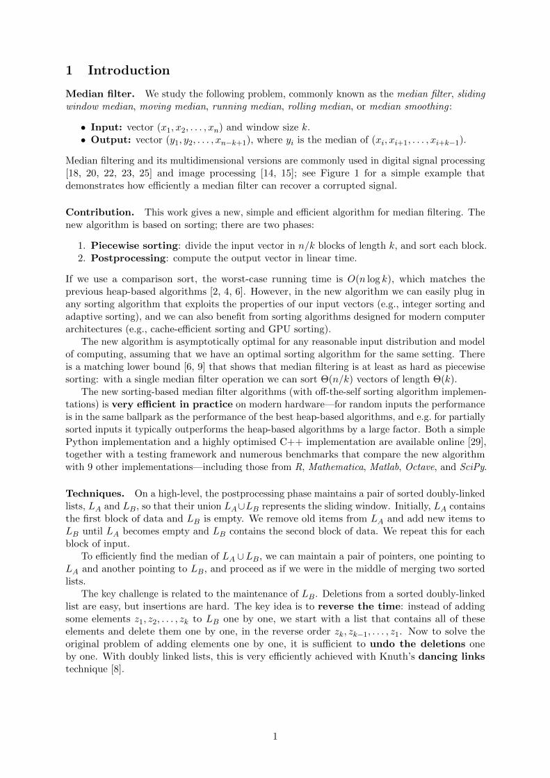
Median filtering and its multidimensional versions are commonly used in digital signal processing[18, 20, 22, 23, 25] and image processing [14, 15]; see Figure 1 for a simple example thatdemonstrates how efficiently a median filter can recover a corrupted signal.

Contribution. This work gives a new, simple and efficient algorithm for median filtering. Thenew algorithm is based on sorting; there are two phases:

1. Piecewise sorting: divide the input vector in n/k blocks of length k, and sort each block.2. Postprocessing: compute the output vector in linear time.

If we use a comparison sort, the worst-case running time is O(n log k), which matches theprevious heap-based algorithms [2, 4, 6]. However, in the new algorithm we can easily plug inany sorting algorithm that exploits the properties of our input vectors (e.g., integer sorting andadaptive sorting), and we can also benefit from sorting algorithms designed for modern computerarchitectures (e.g., cache-efficient sorting and GPU sorting).

The new algorithm is asymptotically optimal for any reasonable input distribution and modelof computing, assuming that we have an optimal sorting algorithm for the same setting. Thereis a matching lower bound [6, 9] that shows that median filtering is at least as hard as piecewisesorting: with a single median filter operation we can sort Θ(n/k) vectors of length Θ(k).

The new sorting-based median filter algorithms (with off-the-self sorting algorithm implemen-tations) is very efficient in practice on modern hardware—for random inputs the performanceis in the same ballpark as the performance of the best heap-based algorithms, and e.g. for partiallysorted inputs it typically outperforms the heap-based algorithms by a large factor. Both a simplePython implementation and a highly optimised C++ implementation are available online [29],together with a testing framework and numerous benchmarks that compare the new algorithmwith 9 other implementations—including those from R, Mathematica, Matlab, Octave, and SciPy.

Techniques. On a high-level, the postprocessing phase maintains a pair of sorted doubly-linkedlists, LA and LB, so that their union LA∪LB represents the sliding window. Initially, LA containsthe first block of data and LB is empty. We remove old items from LA and add new items toLB until LA becomes empty and LB contains the second block of data. We repeat this for eachblock of input.

To efficiently find the median of LA ∪LB, we can maintain a pair of pointers, one pointing toLA and another pointing to LB, and proceed as if we were in the middle of merging two sortedlists.

The key challenge is related to the maintenance of LB. Deletions from a sorted doubly-linkedlist are easy, but insertions are hard. The key idea is to reverse the time: instead of addingsome elements z1, z2, . . . , zk to LB one by one, we start with a list that contains all of theseelements and delete them one by one, in the reverse order zk, zk−1, . . . , z1. Now to solve theoriginal problem of adding elements one by one, it is sufficient to undo the deletions oneby one. With doubly linked lists, this is very efficiently achieved with Knuth’s dancing linkstechnique [8].

1

0.0

0.5

1.0

(a)

0.0

0.5

1.0

(b)

0.0

0.5

1.0

(c)

0 500 1000 1500 2000

0.0

0.5

1.0

(d)

Figure 1: The median filter can recover corrupted data much better than e.g. moving average filters.(a) Original data, n = 2000. (b) 25% of data points corrupted, some random noise added. (c) Movingaverage filter applied, window size k = 25. (d) Median filter applied, window size k = 25. In all figures,the shaded area represents the original data.

2 Prior Work

Algorithms. There is, of course, a trivial algorithm for median filtering in time O(nk): simplyfind the median separately for each window. This approach, together with sorting networks,can be attractive for hardware implementations of median filters [10], but as a general-purposealgorithm it is inefficient.

Non-trivial algorithms presented in the literature are unanimously based on the followingidea: maintain a data structure that represents the sliding window. Such a data structure needsto support three operations: “construct”, “find the median”, and “remove the oldest elementand add a new element”. With such a data structure, one can first construct it with elementsx1, x2, . . . , xk, and then process elements xk+1, xk+2, . . . , xn one by one, in this order. Concreteideas for the implementation of the window data structure can be classified as follows:

1. Data structures for B-bit integers. For a small B, we can easily maintain a histogram with2B buckets. However, to find the new median we need to find an adjacent unoccupiedbucket. The following approaches have been discussed in the literature:

(a) linear scanning [3, 5, 6]: worst-case running time Θ(n2B)(b) binary trees [3, 6]: worst-case running time Θ(nB)(c) van Emde Boas trees [6]: worst-case running time Θ(n logB).

2. Efficient comparison-based data structures with a Θ(n log k) worst-case running time:

(a) a maxheap-minheap pair [2, 4, 6](b) binary search trees [6](c) finger trees [6].

2

3. Inefficient comparison-based data structures with a Θ(nk) worst-case running time:

(a) doubly-linked lists [6](b) sorted arrays [1, 6].

In summary, the search for efficient median filter algorithms has focused on the design of anefficient data structure for the sliding window. While it is known that 2-dimensional medianfiltering can benefit from a clever traversal order [11], it seems that all existing algorithmsfor 1-dimensional median filtering are based on the idea of a doing a single, uniform, in-ordertraversal of the input vector.

It seems that the present work is the first deviation from this trend in the long history ofmedian filtering algorithms. In essence, we see median filtering as an algorithmic challenge—instead of asking how to construct an efficient data structure for the sliding window, we ask howto pre-process the input vector so that the sliding window is much easier to maintain.

Applications and Implementations. Median filtering has been applied in statistical dataanalysis at least since 1920s [7], and it was popularised by Tukey in 1970s [12, Section 7A].

Nowadays, a median filter is a standard subroutine in numerous scientific computing en-vironments and signal processing packages. In R it is called “runmed” [22, p. 1507], and inMathematica it is called “MedianFilter” [25]. Matlab’s Signal Processing Toolbox, GNU Octave’s“signal” package, and SciPy ’s module “scipy.signal” all provide a median filter function called“medfilt1” [18, 20, 23].

Multidimensional generalisations of the median filter are commonly used in image processing.For example, in Photoshop there is a noise reduction filter called “Median” [14], and in Gimpthere is a “Despeckle” filter, which is a generalisation of the 2-dimensional median filter [15].

Surprisingly, most of the existing implementations of the median filter in scientific comput-ing environments are very inefficient for a large k. The experiments conducted in this workdemonstrate that the median filter functions in the current versions of Matlab, Mathematica,Octave, and SciPy all exhibit approximately Θ(nk) complexity for random inputs (see Figure 8for examples). It should be noted that these software packages typically provide very efficientroutines for sorting, which would make the algorithm presented in this work relatively easy toimplement.

The only major software package with an efficient Θ(n log k) median filter implementationseems to be R. For large values of k, the runmed function in R applies a high-quality implemen-tation of the double-heap data structure [2, 4, 6]. The end result is very efficient both in theoryand in practice, for a wide range of n and k (see Figures 8 and 9 for examples).

We are aware of only one general-purpose median filter implementation that consistentlyoutperforms R: an open source C implementation by AShelly from 2011 [26, 27]. This is, again,an implementation of the double-heap technique. Raffel [28] has adapted this implementation toC++, and we will use Raffel’s version as a baseline in our experiments.

Lower Bounds. There is a simple argument that shows that median filtering is at least asdifficult as piecewise sorting—see, e.g., Juhola et al. [6] and Krizanc et al. [9]. Assume thatk = 2h+ 1, and assume that we want to sort n/(3h+ 2) blocks of size h+ 1. Construct the inputvector x so that before each block we have h times the value −∞ and after each block we have htimes the value +∞. If we now apply the median filter, it is easy to see that in the output eachblock is sorted.

Hence with some linear-time preprocessing and postprocessing, and O(1) invocations of themedian filter operation, we can sort n/k blocks of length k. This work shows that the converseis also true.

3

unwind(B)

B ← construct(X0, P0)

undelete(B)delete(A)

X0

A ← B

A ← B

delete(A)

A ← B

delete(A)

input blocks

output blocks

B ← construct(X1, P1)

B ← construct(X2, P2)

B ← construct(X3, P3)

X1 X2 X3

P0

permutations

P1 P2 P3

Piecewise sorting

Post-processing

Input

Y0

Y1

Y2

Y3

unwind(B)

undelete(B)

unwind(B)

undelete(B)

print

print

print

print

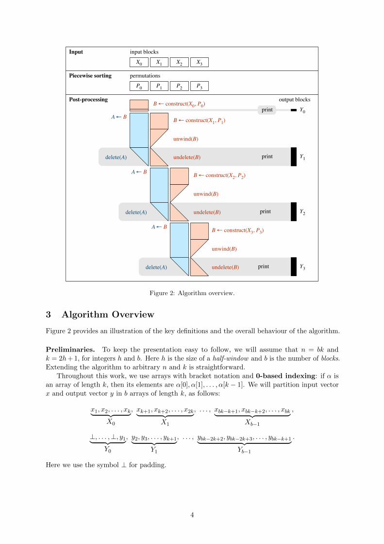
Figure 2: Algorithm overview.

3 Algorithm Overview

Figure 2 provides an illustration of the key definitions and the overall behaviour of the algorithm.

Preliminaries. To keep the presentation easy to follow, we will assume that n = bk andk = 2h+ 1, for integers h and b. Here h is the size of a half-window and b is the number of blocks.Extending the algorithm to arbitrary n and k is straightforward.

Throughout this work, we use arrays with bracket notation and 0-based indexing: if α isan array of length k, then its elements are α[0], α[1], . . . , α[k − 1]. We will partition input vectorx and output vector y in b arrays of length k, as follows:

x1, x2, . . . , xk︸ ︷︷ ︸X0

, xk+1, xk+2, . . . , x2k︸ ︷︷ ︸X1

, . . . , xbk−k+1, xbk−k+2, . . . , xbk︸ ︷︷ ︸Xb−1

,

⊥, . . . ,⊥, y1︸ ︷︷ ︸Y0

, y2, y3, . . . , yk+1︸ ︷︷ ︸Y1

, . . . , ybk−2k+2, ybk−2k+3, . . . , ybk−k+1︸ ︷︷ ︸Yb−1

.

Here we use the symbol ⊥ for padding.

4

Piecewise Sorting. For each j, find a permutation Pj of {0, 1, . . . , k − 1} that sorts theelements of array Xj . That is, for all 0 ≤ s < t < k we have Xj [Pj [s]] ≤ Xj [Pj [t]].

Postprocessing. The first output array Y0 is trivial to compute: its only element is Y0[k−1] =X0[P0[h]]. Let us now focus on the case of 1 ≤ j < b. Define

αA = Xj−1, αB = Xj , πA = Pj−1, πB = Pj , β = Yj .

We will show how to find β in time O(k) given αA, αB, πA, and πB.The basic idea is simple: We maintain sorted doubly-linked lists LA and LB, so that their

union LA ∪ LB represents the sliding window. Initially, LA contains the elements of block αA inan increasing order while LB is empty. At each time step t = 0, 1, . . . , k − 1, we remove elementαA[t] from LA, and add element αB[t] to LB—we will shortly see how to do this efficiently. Inthe end, LA will be empty and LB will contain the elements of αB in an increasing order. Weaugment the data structures LA and LB with additional pointers so that we can efficiently findthe median of LA ∪ LB after each time step t.

The key challenge is related to the maintenance of the linked lists LA and LB . At first, thereseems to be inherent asymmetry:

• Maintenance of LA is easy: we only need to remove elements from a doubly-linked list.• Maintenance of LB is hard: we have to add elements in the right place to keep LB sorted.

The key insight is that the situation is symmetric with respect to time.

4 Main Ingredient: Time Reversal and Dancing Links

Recall that our goal is to efficiently solve the following task, so that at each point list L is asorted doubly-linked list:

(P1) insert α[0], α[1], . . . , α[k − 1] into L one by one

If we reverse the time, our original process becomes

(P2) delete α[k − 1], α[k − 2], . . . , α[0] from L one by one.

Finally, to recover the original process, we reverse the time again, obtaining

(P3) undo the deletions of α[0], α[1], . . . , α[k − 1] one by one.

While (P1) looks difficult to implement, (P2) is easy to solve, and then (P3) can be solved withKnuth’s dancing links technique [8].

We will now explain this idea in more detail. Let us first fix the representation that we willuse for linked lists. For list L, we will maintain two arrays of indexes, ‘prev’ and ‘next’. If α[i] isin list L, then prev[i] is the index of the predecessor of α[i] and next[i] is the successor of α[i].

Given a permutation π that sorts α, we can easily initialise prev and next so that L containsall elements of α in a sorted order; this takes O(k) time. Deletions are also easy: to deleteelement α[i] from L, we simply set

prev[next[i]]← prev[i], next[prev[i]]← next[i]. (1)

Knuth’s [8] observation is that (1) is easy to reverse:

prev[next[i]]← i, next[prev[i]]← i. (2)

In essence, index i and pointers prev[i] and next[i] contain enough information to perfectly undothe deletion of α[i] from list L.

5

α6

α0 α1 α2 α3 α4 α5

3

α:

π : 2 0 5 1 4

α0 α1α2α3 α4α5

prev:

next:

2 3 k5 6 0

5 0 26 k 1

4

3

L:S L \ S

α6

6

1

4

α6

5m:

s = 3α0 α1α2α3 α4α5

2 3 k5 1 0

5 0 24 k 1

4

3

S L \ S

1

4

5m:

s = 3

delete(6),advance

undelete(6)

α0 α1 α2 α3 α4 α5

3 2 0 5 1 4

α6

6

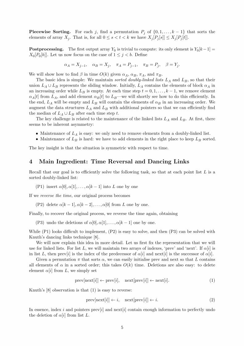
Figure 3: An example of the behaviour of the block data structure.

Hence we can do the following:

1. Construct the sorted list L with the help of permutation π.2. Unwind the list by deleting α[k − 1], α[k − 2], . . . , α[0] in this order. Now list L is empty.3. At each time step t = 0, 1, . . . , k − 1, undo the deletion of element α[t]. In effect, we

insert α[t] in the sorted doubly-linked list L in the right position.

The simple idea of combining piecewise sorting, time reversals, and dancing links is all that ittakes to design an efficient median filter algorithm. The rest of this work presents the algorithmin more detail.

5 Block Data Structure

The algorithm relies on block data structures (see Figure 3). Conceptually, a block data structureB is a tuple (αB, πB, LB, sB), where array αB is one block of input, array πB is the permutationthat sorts αB, list LB contains some subset of the elements of αB, and sB is a counter between 0and |LB|. We say that the first sB elements of list LB are small, and the rest of the elements arelarge. We will omit subscript B when it is clear from the context.

When a block data structure is created, list LB will contain all k = 2h+ 1 elements of αB,and the first h of them will be small. We can then delete elements, undo deletions, and adjust sB.

5.1 Interface

The block data structure B supports the operations shown in Figure 4. The time complexity ofconstruct and unwind is O(k), and for all other operations it is O(1). Deletions and undeletionsmust be properly nested. For example, this sequence of operations is permitted:

delete(B, 15), delete(B, 3), undelete(B, 3),undelete(B, 15).

However, this sequence of operations is not permitted:

delete(B, 15), delete(B, 3), undelete(B, 15), undelete(B, 3).

6

construct(α, π): Return B = (α, π, L, s), where:

L =(α[π[0]], α[π[1]], . . . , α[π[k − 1]]

)s = h

delete(B, i): Remove α[i] from L

s← max {0, s− 1}

undelete(B, i): Put α[i] back to L

unwind(B): delete(B, k − 1),delete(B, k − 2), . . . ,delete(B, 0)

advance(B): s← s+ 1

small(B): Return s

peek(B): Return the first large element, or +∞ if all elements are small

Figure 4: Block data structure interface.

5.2 Assumption: Stable Sorting

For convenience, we will assume that permutation π is a stable sort of input α. In practice,we can very efficiently find such a π as follows: construct an array of pairs (α[i], i), sort it inlexicographic order with any sorting algorithm, and then pick the second element of each pair.This way we have constructed π and also guaranteed stability.

We could also do without a stable sort if we slightly modified the algorithm. In essence,we could first construct the inverse permutation π−1 and then use π−1[i] instead of (α[i], i) incomparisons.

5.3 Implementation

To implement the block data structure B, we will use the following fields in addition to input α,permutation π, and counter s (see Figure 3):

• prev, next: arrays of length k + 1,• m: integer between 0 and k.

Assume that L = (α[p0], α[p1], . . . , α[pc−1]). For convenience, let p−1 = pc = k. We will maintainthe following invariants:

• next[k] = p0 and next[pi] = pi+1 for all i,• prev[k] = pc−1 and prev[pi] = pi−1 for all i,• m = ps.

Define α[k] = +∞. Given any index i with α[i] ∈ L, it is easy to check if α[i] is small: see if(α[i], i) < (α[m],m) in lexicographic order—recall that we assumed that this is compatible withpermutation π.

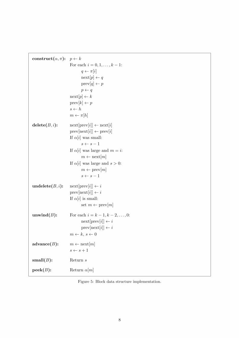
We are now ready to explain how to implement each operation; the algorithm is given inFigure 5. While some care is needed in the corner cases (e.g., m = k or i = m), it is relativelyeasy to verify that the invariants are maintained and that the implementation is correct.

6 Complete Algorithm

We will now present the complete sorting-based median filter algorithm. Recall that n = bk andk = 2h+ 1. The input vector x is partitioned in arrays X0, X1, . . . , Xb−1.

7

construct(α, π): p← k

For each i = 0, 1, . . . , k − 1:

q ← π[i]

next[p]← q

prev[q]← p

p← q

next[p]← k

prev[k]← p

s← h

m← π[h]

delete(B, i): next[prev[i]]← next[i]

prev[next[i]]← prev[i]

If α[i] was small:

s← s− 1

If α[i] was large and m = i:

m← next[m]

If α[i] was large and s > 0:

m← prev[m]

s← s− 1

undelete(B, i): next[prev[i]]← i

prev[next[i]]← i

If α[i] is small:

set m← prev[m]

unwind(B): For each i = k − 1, k − 2, . . . , 0:

next[prev[i]]← i

prev[next[i]]← i

m← k, s← 0

advance(B): m← next[m]

s← s+ 1

small(B): Return s

peek(B): Return α[m]

Figure 5: Block data structure implementation.

8

postprocess(X,P ): B ← construct(X0, P0)

Print peek(B) (‡)For each j = 1, 2, . . . , b− 1:

A← B

B ← construct(Xj , Pj)

unwind(B)

For each i = 0, 1, . . . , k − 1:

delete(A, i) (†)undelete(B, i)

If small(A) + small(B) < h:

If peek(A) ≤ peek(B):

advance(A)

Otherwise:

advance(B)

Print min{peek(A), peek(B)} (

†

)

Figure 6: Algorithm for median filtering: postprocessing phase.

6.1 Preprocessing

For each j, find a permutation Pj that sorts the elements of Xj . As discussed in Section 5.2, wewill assume a stable sort.

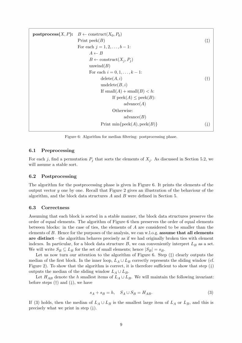
6.2 Postprocessing

The algorithm for the postprocessing phase is given in Figure 6. It prints the elements of theoutput vector y one by one. Recall that Figure 2 gives an illustration of the behaviour of thealgorithm, and the block data structures A and B were defined in Section 5.

6.3 Correctness

Assuming that each block is sorted in a stable manner, the block data structures preserve theorder of equal elements. The algorithm of Figure 6 then preserves the order of equal elementsbetween blocks: in the case of ties, the elements of A are considered to be smaller than theelements of B. Hence for the purposes of the analysis, we can w.l.o.g. assume that all elementsare distinct—the algorithm behaves precisely as if we had originally broken ties with elementindexes. In particular, for a block data structure B, we can conveniently interpret LB as a set.We will write SB ⊆ LB for the set of small elements; hence |SB| = sB.

Let us now turn our attention to the algorithm of Figure 6. Step (‡) clearly outputs themedian of the first block. In the inner loop, LA ∪ LB correctly represents the sliding window (cf.Figure 2). To show that the algorithm is correct, it is therefore sufficient to show that step (

†

)outputs the median of the sliding window LA ∪ LB.

Let HAB denote the h smallest items of LA ∪ LB. We will maintain the following invariant:before steps (†) and ( †), we have

sA + sB = h, SA ∪ SB = HAB. (3)

If (3) holds, then the median of LA ∪ LB is the smallest large item of LA or LB, and this isprecisely what we print in step (

†

).

9

We will now argue that the invariant indeed holds throughout the algorithm. Let us firstmake some easy observations:

1. Invariant (3) holds before step (†) for iteration j = 1 and i = 0.

2. Assume that invariant (3) holds after step ( †) for some iteration j = j0 and i = i0 < k − 1.Then it holds before step (†) for iteration j = j0 and i = i0 + 1.

3. Assume that invariant (3) holds after step ( †) for some iteration j = j0 < b−1 and i = k−1.Then it holds before step (†) for iteration j = j0 + 1 and i = 0.

The nontrivial part is covered in the following lemma.

Lemma 1. Assume that invariant (3) holds before step (†) for some iteration j = j0 and i = i0.Then it holds before step (

†

) for the same iteration j = j0 and i = i0.

Proof. We will use the following convention to refer to the states of block data structures Aand B:

• A and B to refer to the original states before step (†),• A and B to refer to the new states after delete and undelete operations,• A and B to refer to the new states before step (

†

).

First, assume that SA = ∅. Then all elements of LA are strictly larger than any element ofSB = HAB. If αB[i] is large, undelete(B, i) does not change SB; if αB[i] is small, undelete(B, i)replaces the largest element of SB with αB[i]. In both cases, sB = h and therefore A = A andB = B. We conclude that

SA = ∅, SB = HAB.

Second, assume that SA 6= ∅. In this case the delete(A, i) operation decreases the size of SA,and we have

sA = sA − 1, sB = sB, sA + sB = h− 1.

Hence we will perform one advance operation, after which sA + sB = h. However, it is notentirely obvious that this results in SA ∪ SB = HAB, too. To prove this, some case analysis isneeded. The critical elements are

aA = αA[i], pA = maxSA, qA = min(LA \ SA),

aB = αB[i], pB = maxSB, qB = min(LB \ SB).

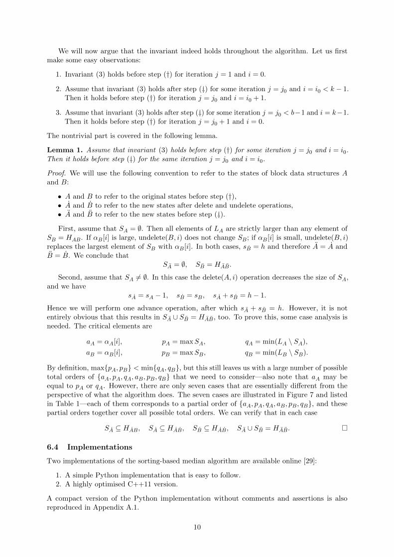
By definition, max{pA, pB} < min{qA, qB}, but this still leaves us with a large number of possibletotal orders of {aA, pA, qA, aB, pB, qB} that we need to consider—also note that aA may beequal to pA or qA. However, there are only seven cases that are essentially different from theperspective of what the algorithm does. The seven cases are illustrated in Figure 7 and listedin Table 1—each of them corresponds to a partial order of {aA, pA, qA, aB, pB, qB}, and thesepartial orders together cover all possible total orders. We can verify that in each case

SA ⊆ HAB, SA ⊆ HAB, SB ⊆ HAB, SA ∪ SB = HAB.

6.4 Implementations

Two implementations of the sorting-based median algorithm are available online [29]:

1. A simple Python implementation that is easy to follow.2. A highly optimised C++11 version.

A compact version of the Python implementation without comments and assertions is alsoreproduced in Appendix A.1.

10

after delete/undeleteafter advance

SB

SA

SB

SA

SB

SA

SA

SB

SA

SB

SA

SB

SB

SA

aA pA qA

aB pB qB

aA pA qA

aBpB qB

aA pA qA

aBpB qB

aA pA qA

aBpB

qB

aA

pA qA

aB

pB qB

aA

pA qA

aB pB qB

aApA qA

aB pB qB

Before delete/undelete

After delete/undelete + advance

SB

SA pA qA

pB qB

Figure 7: Case analysis in the proof of Lemma 1. Here aA is the element that we delete from A with thedelete(A, i) operation, and aB is the element that we add to B with the undelete(B, i) operation. Finally,we apply either advance(A) or advance(B). See also Table 1.

Partial order HAB SA SB SA SB

aA < pA

aB < pB HAB − aA + aB SA − aA SB − pB + aB SA SB + pBpB < aB < min{qA, qB} HAB − aA + aB SA − aA SB SA SB + aBqB < min{qA, aB} HAB − aA + qB SA − aA SB SA SB + qBqA < min{qB, aB} HAB − aA + qA SA − aA SB SA + qA SB

pa ≤ aA

pB < aB HAB SA − pA SB SA + pA SBaB < pB < pA HAB − pA + aB SA − pA SB − pB + aB SA SB + pBmax{aB, pA} < pB HAB − pB + aB SA − pA SB − pB + aB SA + pA SB

Table 1: Case analysis in the proof of Lemma 1. We use the shorthand notation U + e = U ∪ {e} andU − e = U \ {e}. See Figure 7 for illustrations.

11

7 Experiments

We will now present the experiments in which we compare the performance of the new sorting-based median filter algorithm with 9 other implementations of median filter algorithms,including the median filter functions from R, Matlab, GNU Octave, SciPy, and Mathematica.It turns out that our sorting-based median filter algorithm performs consistently very well incomparison with the other implementations.

For a broad range of window sizes (between h = 10 and h = 5 · 107) and for various inputdistributions, our implementation never loses by more than 20 % in comparison with the fastestmedian filter algorithm from prior work. In many cases, our algorithm outperforms all competingimplementations by a large factor—by a factor up to 3 for uniform random inputs and by afactor up to 8 for more benign input distributions.

7.1 Implementations

We will now describe the 11 implementations that we benchmarked. We start with our newalgorithm and two simple baseline algorithms—all of these are optimised C++11 implementations:

SortMedian: The sorting-based median algorithm described in this work. For sorting, we usestd::sort from the C++ standard library.

TreeMedian: The sliding window is maintained as a pair of balanced search trees. We usestd::multiset from the C++ standard library—this is typically a highly optimised imple-mentation of a red-black tree.

MoveMedian: The sliding window is maintained as a sorted array. Binary search is used tolocate the part of the array that needs to be moved in order to accommodate the newelement. Standard library routines std::copy and std::copy backward are used to efficientlymove a block of data.

We have also included an efficient open source median filter implementation in our testingframework—while the algorithm idea dates back to 1980s, this is a modern C++ implementationfrom 2011:

HeapMedian: The sliding window is maintained as a double heap [2, 4, 6]. This is Raffel’sadaptation [28] of AShelly’s implementation [26, 27], with very minor modifications.

The source code of the above algorithms, as well as a unified testing framework, is availableonline [29]. To ensure correctness, there is also a verification tool that compares the outputs ofall four implementations against each other.

In addition to these C++ implementations, we also benchmark median filter routines thatare available in the following scientific computing environments and signal processing packages:

• R [21], a free software for statistical computing,• Matlab [17], a commercial numerical computing environment,• GNU Octave [19], a free numerical computing environment,• SciPy [16], a collection of Python modules for scientific computing,• Mathematica [24], a commercial symbolic computing environment.

In total, six algorithm implementations were benchmarked:

R, runmed(“Turlach”): The standard routine “runmed” [22, p. 1507] in R, with parameter“algorithm” set to “Turlach”. This implementation maintains the sliding window as a doubleheap.

R, runmed(“Stuetzle”): As above, but with parameter “algorithm” set to “Stuetzle”. Thisimplementation maintains the sliding window as a sorted array.

12

Octave, medfilt1: Function “medfilt1” [20] in GNU Octave’s “signal” package. Based on thesource code, this function maintains a sorted array.

Matlab, medfilt1: Function “medfilt1” [18] in Matlab. Based on the source code, this functionfinds the median separately for each possible location of the sliding window.

SciPy, scipy.signal.medfilt: Function “scipy.signal.medfilt” [23] in SciPy. Based on the sourcecode, this function finds the median by sorting the sliding window.

Mathematica, MedianFilter: Function “MedianFilter” [25] in Mathematica. No source codeor information on the algorithm is publicly available.

Finally, to be fair with software packages that rely on median filter implementations written inhigh-level languages, we also tested a very slow implementation of our sorting-based algorithm:

SortMedian.py: The simple Python implementation from Appendix A.1.

7.2 Comparison of All Implementations

We will start with a broad comparison of all 11 implementations described in Section 7.1. Theexperiments were conducted as follows (with a few exceptions, see below):

• We keep bh fixed and vary h. This is approximately equivalent to keeping the size of inputvector n = (2h+ 1)b fixed and varying the window size k = 2h+ 1.

• Input consists of independent, uniformly distributed, random 32-bit integers, or its closestequivalent that is supported in the computing environment that we benchmark.

• Each experiment was ran 10 times with different random seeds.

• The plots report the median running times.

• The experiments were ran on the same OS X computer equipped with a 1.7 GHz IntelCore i7 processor and 8 GB of RAM.

The following exceptions were made:

• Mathematica: Only 1 experiment was ran, as this was by far the slowest implementation.

• Matlab: This implementation required huge amounts of memory. In the end, we resorted toa high-end Linux computer equipped with a 2.8 GHz Intel Xeon processor and 256 GB ofRAM. Only 1 experiment was ran, as this is clearly not among the fastest implementations.

• R: The running times of the fastest experiments (below 10 ms) are averages of 10 or 100trials.

Detailed information on the software versions and computing platforms is given in Table 2. Thesource code of the test suite and the raw test results are available online [29].

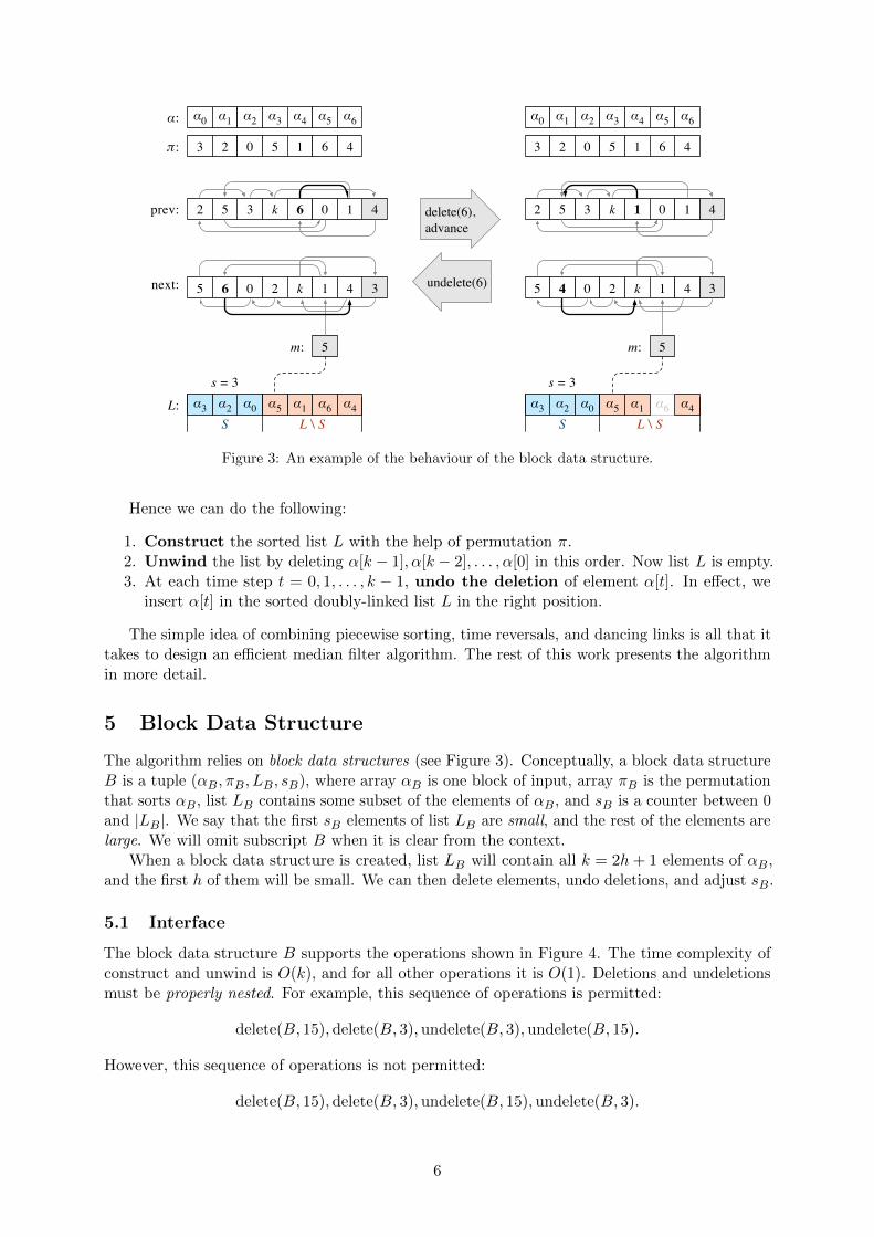
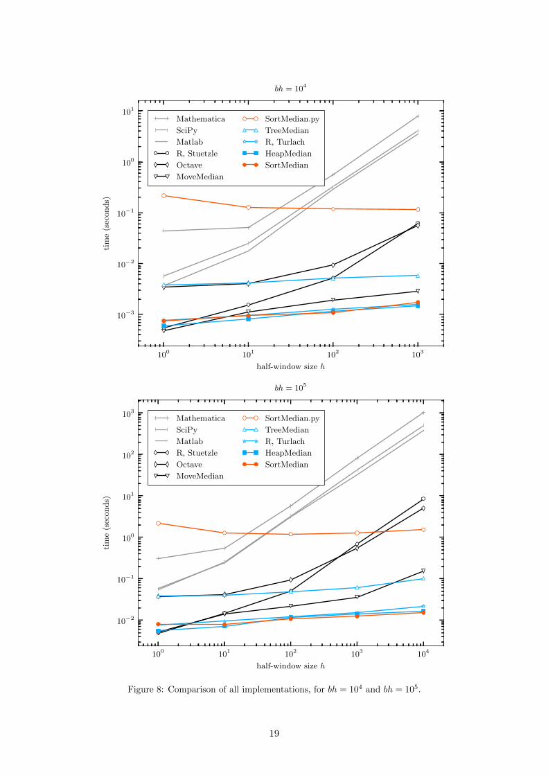
First we ran experiments with small parameter values bh = 104 and bh = 105 for allimplementations; the results are reported in Figure 8 in the appendix. From the log-log plots itis easy to see that most of the implementations exhibit running times that are approximatelyproportional to nk. Only four implementations provide a decent performance and scalability:SortMedian, HeapMedian, TreeMedian, and R’s “Turlach” implementation.

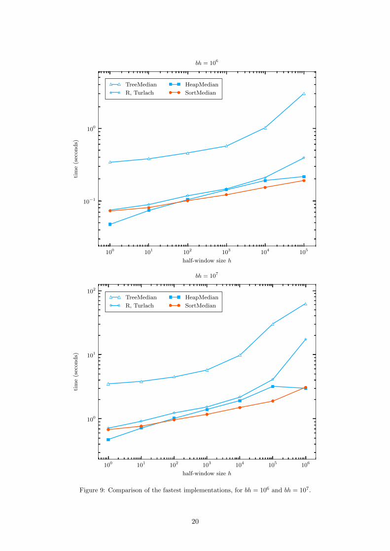
Then we repeated the experiments with the most promising implementations for largerparameter values bh = 106 and bh = 107. The results are reported in Figure 9. The key findingis that SortMedian and HeapMedian consistently outperform all other implementations for largeinputs. In the next section, we will focus on these two implementations.

13

Software Function Versions Platform

R [21] runmed [22] R 3.1.0 OS X

Octave [19] medfilt1 [20] GNU Octave 3.8.1 OS Xsignal 1.3.0

Matlab [17] medfilt1 [18] Matlab R2014a (8.3.0.532) Linux

SciPy [16] scipy.signal.medfilt [23] Python 2.7.7 OS Xnumpy 1.8.1scipy 0.14.0

Mathematica [24] MedianFilter [25] Mathematica 9.0.1.0 OS X

OS X: Intel Core i7, 1.7 GHz, 8 GB RAM.

Linux: Intel Xeon, 2.8 GHz, 256 GB RAM.

Table 2: The software versions and platforms used in the experiments of Section 7.2 and Figures 8–9.

7.3 Comparison of HeapMedian and SortMedian

We will now do a more detailed comparison of the fastest algorithms, HeapMedian and SortMedian.These tests were conducted as follows:

• We keep bh fixed and vary h. In total, we use 66 different combinations of h and b.

• We use 2 different versions of the implementations: one for 32-bit inputs and one for 64-bitinputs.

• We use 7 different generators to produce the input array x:

1. asc: ascending values, x[i] = i.2. desc: descending values, x[i] = n− i.3. r-asc: ascending values + small uniform random noise, i ≤ x[i] < i+ 104.4. r-desc: descending values + small uniform random noise, n− i ≤ x[i] < n− i+ 104.5. r-large: large uniform random integers (32-bit or 64-bit).6. r-small : small uniform random integers, 0 ≤ x[i] < 104.7. r-block : piecewise constant data + small uniform random noise.

• For each combination of a version and a generator, we run the experiment for 5 times, withdifferent random seeds.

• The plots report the median (solid curve) and the region from the 2nd decile to the 9thdecile (shading). That is, the shaded area represents 80 % of the experiments.

• The experiments were ran on Linux, using the Intel Xeon nodes of the Triton cluster [13],with one processor allocated for each experiment.

• To compile the code, we used GCC version 4.8.2 and GCC’s implementation of the C++standard library (a.k.a. libstdc++).

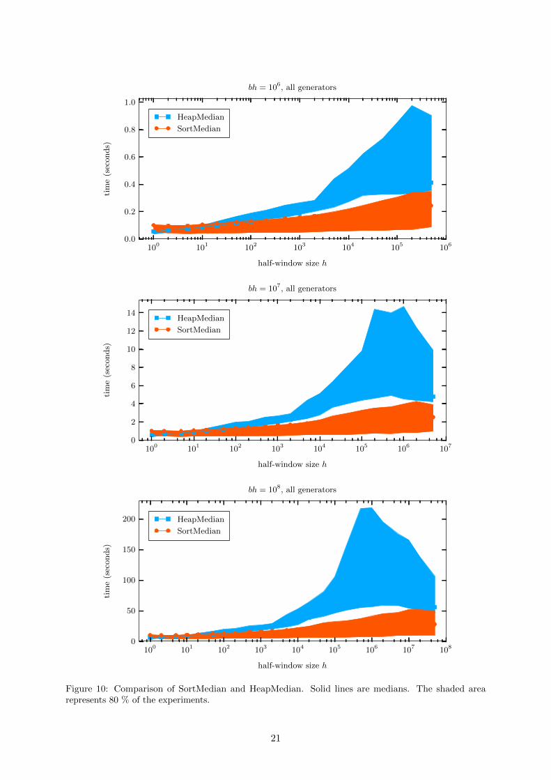
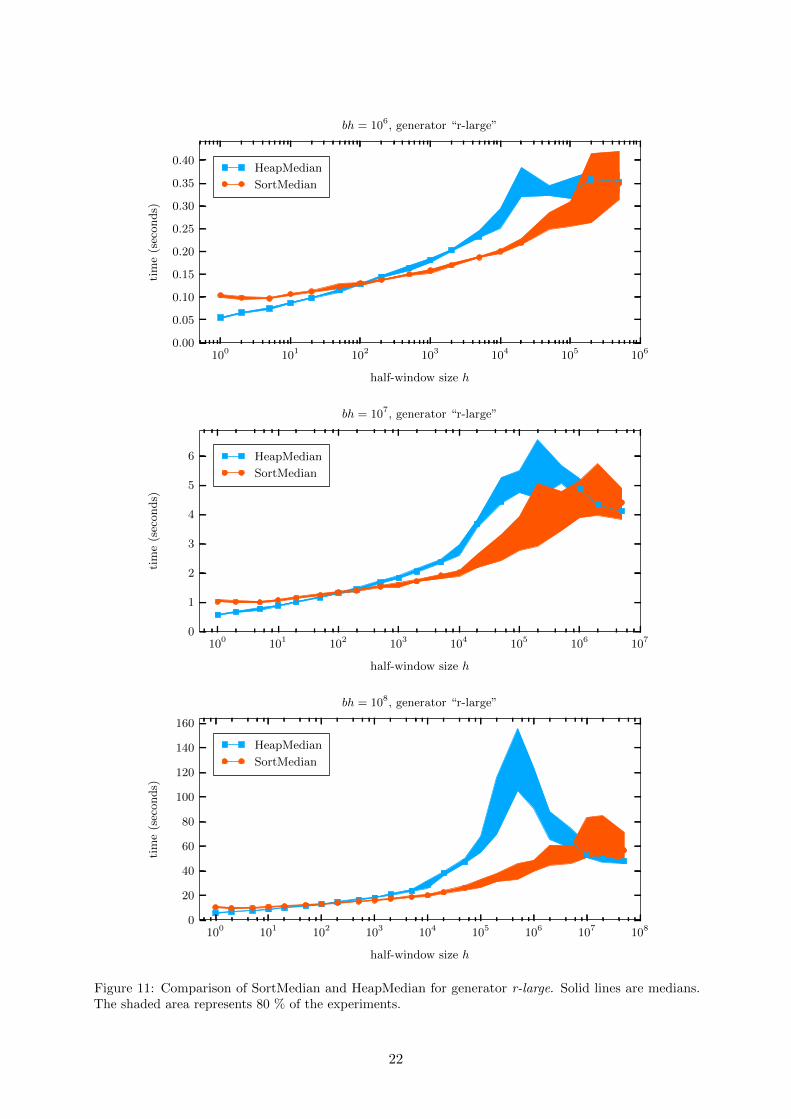
In total, this setup results in 66× 2× 7× 5 = 4620 experiments per algorithm. The full sourcecode and the raw test results are available online [29]. An overview of the results is given inFigure 10 in the appendix, and selected examples of generator-specific results are shown inFigures 11–13. Note that the y axis is linear in these plots.

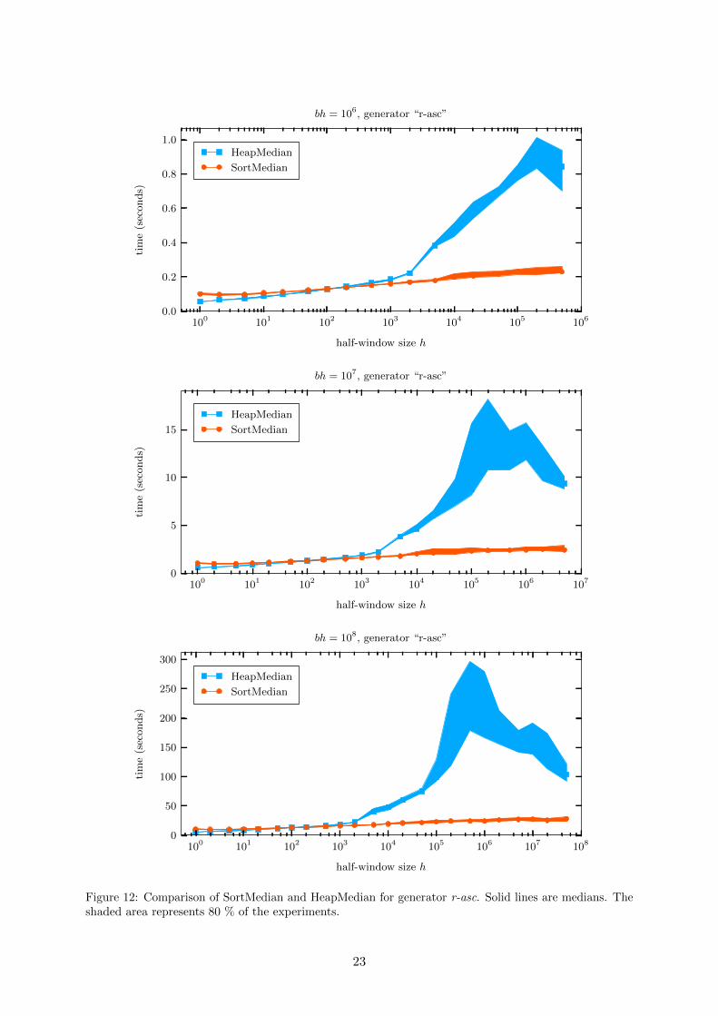
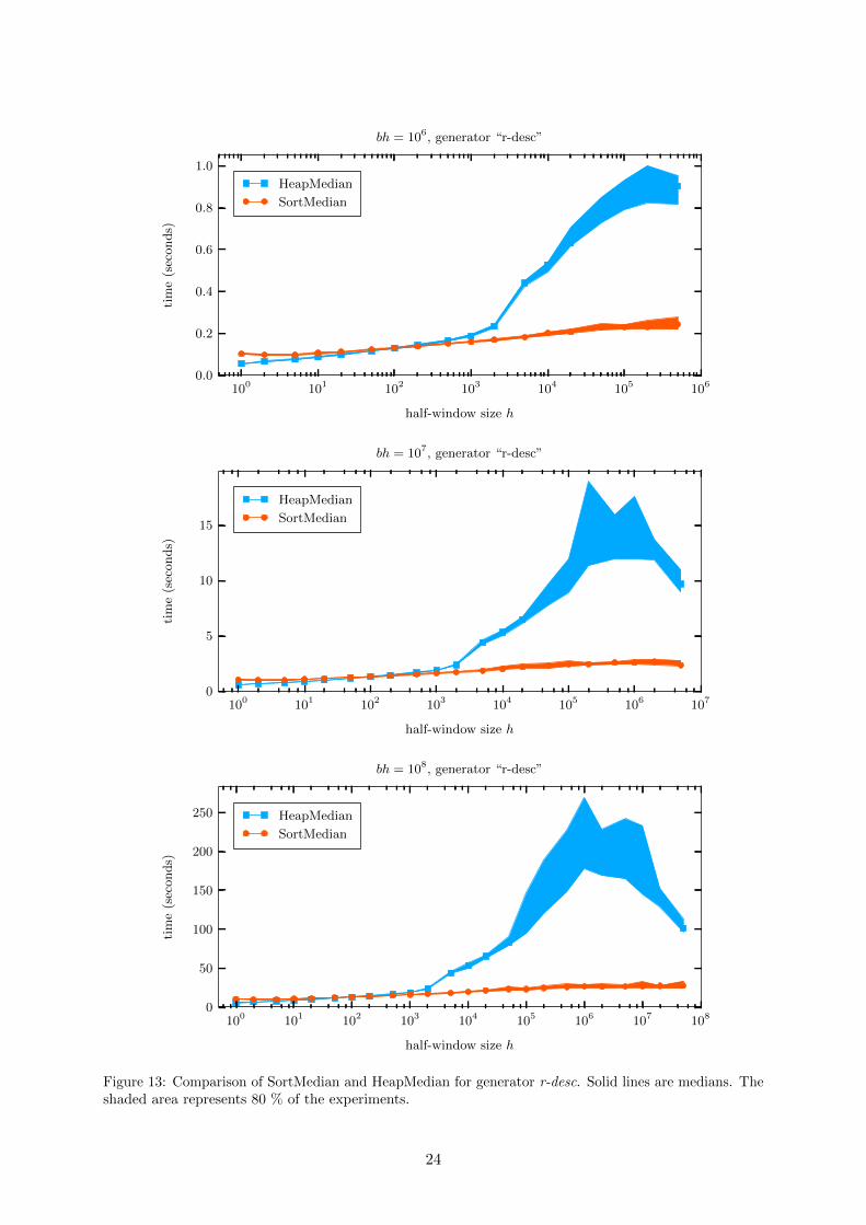
As we can see from the plots, SortMedian typically performs better than HeapMedian. Therunning times are consistently low. HeapMedian is a clear winner only for very small windowsizes, while SortMedian typically wins by a large factor for larger windows.

14

One the most interesting findings is shown in Figures 12 and 13. These plots demonstratethat SortMedian makes a very effective use of partially sorted inputs, while such inputs areactually more difficult for HeapMedian than uniform random inputs. Perhaps the most importantfactor here is the locality of memory references and cache efficiency.

Acknowledgements

Computer resources were provided by the Aalto University School of Science “Science-IT”project [13]. Many thanks to David Eppstein, Geoffrey Irving, Petteri Kaski, Pat Morin, andSaeed for comments and discussions. This problem has been discussed online on TheoreticalComputer Science Stack Exchange [30] and Google+ [31].

References

[1] M. Omair Ahmad and Duraisamy Sundararajan. A fast algorithm for two-dimensionalmedian filtering. IEEE Transactions on Circuits and Systems, 34(11):1364–1374, 1987.doi:10.1109/TCS.1987.1086059.

[2] Jaakko T. Astola and T. George Campbell. On computation of the running median.IEEE Transactions on Acoustics, Speech, and Signal Processing, 37(4):572–574, 1989. doi:10.1109/29.17539.

[3] E. Ataman, V. K. Aatre, and K. M. Wong. A fast method for real-time median filtering.IEEE Transactions on Acoustics, Speech, and Signal Processing, 28(4):415–421, 1980. doi:10.1109/TASSP.1980.1163426.

[4] W. Hardle and W. Steiger. Algorithm AS 296: Optimal median smoothing. Applied Statistics,44(2):258, 1995. doi:10.2307/2986349.

[5] Thomas S. Huang, George J. Yang, and Gregory Y. Tang. A fast two-dimensional medianfiltering algorithm. IEEE Transactions on Acoustics, Speech, and Signal Processing, 27(1):13–18, 1979. doi:10.1109/TASSP.1979.1163188.

[6] Martti Juhola, Jyrki Katajainen, and Timo Raita. Comparison of algorithms for standardmedian filtering. IEEE Transactions on Signal Processing, 39(1):204–208, 1991. doi:10.1109/78.80784.

[7] W. Willford I. King. An improved method for measuring the seasonal factor. Journal ofthe American Statistical Association, 19(147):301–313, 1924. doi:10.1080/01621459.1924.10502887.

[8] Donald E. Knuth. Dancing links. In Jim Davies, Bill Roscoe, and Jim Woodcock, editors,Millennial Perspectives in Computer Science: Proceedings of the 1999 Oxford–MicrosoftSymposium in Honour of Sir Tony Hoare, Cornerstones of Computing, pages 187–214.Palgrave Macmillan, 2000. arXiv:cs/0011047.

[9] Danny Krizanc, Pat Morin, and Michiel Smid. Range mode and range median queries onlists and trees. Nordic Journal of Computing, 12(1):1–17, 2005.

[10] Kemal Oflazer. Design and implementation of a single-chip 1-D median filter. IEEETransactions on Acoustics, Speech, and Signal Processing, 31(5):1164–1168, 1983. doi:10.1109/TASSP.1983.1164203.

[11] Simon Perreault and Patrick Hebert. Median filtering in constant time. IEEE Transactionson Image Processing, 16(9):2389–2394, 2007. doi:10.1109/TIP.2007.902329.

[12] John W. Tukey. Exploratory Data Analysis. Addison-Wesley, Reading, MA, 1977.

15

Software and Hardware

[13] Science-IT. Aalto University, School of Science, July 2012. http://sci.aalto.fi/en/research/muu tutkimustoiminta/science-it/, accessed 2014-06-05.

[14] Adobe. Photoshop CS 6 Help, Filter effects reference, 2014. https://helpx.adobe.com/photoshop/using/filter-effects-reference.html, accessed 2014-06-05.

[15] GIMP Documentation Team. GNU Image Manipulation Program, Enhance filters, Despeckle,2014. http://docs.gimp.org/en/plug-in-despeckle.html, accessed 2014-06-05.

[16] Eric Jones, Travis Oliphant, Pearu Peterson, et al. SciPy: Open source scientific tools forPython, 2001–2014. http://www.scipy.org/, accessed 2014-06-05.

[17] MathWorks. MATLAB R2014a. Natick, Massachusetts, 2014.

[18] MathWorks. MATLAB Signal Processing Toolbox, medfilt1. Natick, Massachusetts, 2014.http://www.mathworks.se/help/signal/ref/medfilt1.html, accessed 2014-06-05.

[19] Octave community. GNU Octave 3.8.1, 2014. http://www.gnu.org/software/octave/.

[20] Octave community. Octave signal package, medfilt1, January 2014. http://octave.sourceforge.net/signal/function/medfilt1.html, accessed 2014-06-05.

[21] R Core Team. R: A Language and Environment for Statistical Computing. R Foundationfor Statistical Computing, Vienna, Austria, 2014. http://www.r-project.org/.

[22] R Core Team. R: A Language and Environment for Statistical Computing, Reference Index,Version 3.1.0. Vienna, Austria, April 2014. http://cran.r-project.org/doc/manuals/r-release/fullrefman.pdf, accessed 2014-06-05.

[23] Scipy Community. SciPy Reference Guide, Signal Processing, scipy.signal.medfilt, May2014. http://docs.scipy.org/doc/scipy/reference/generated/scipy.signal.medfilt.html, accessed2014-06-05.

[24] Wolfram. Mathematica 9. Champaign, Illinois, 2012.

[25] Wolfram. Mathematica 9 Documentation Center, MedianFilter. Champaign, Illinois, 2014.https://reference.wolfram.com/mathematica/ref/MedianFilter.html, accessed 2014-06-05.

Online Forums and Code Repositories

[26] AShelly. mediator.c. GitHub, 2011. https://gist.github.com/ashelly/5665911, last modified2013-05-28, accessed 2014-06-05.

[27] AShelly. Rolling median in C – Turlach implementation. StackOveflow, May 2011. http://stackoverflow.com/a/5970314, last modified 2013-05-30, accessed 2014-06-05.

[28] Colin Raffel. median-filter. GitHub, 2012. https://github.com/craffel/median-filter, lastmodified 2012-12-21, accessed 2014-05-20.

[29] Jukka Suomela. Median filter, version 2014-06-05. ZENODO, 2014. doi:10.5281/zenodo.10325. Also available on https://github.com/suomela/median-filter and https://bitbucket.org/suomela/median-filter.

[30] Jukka Suomela, David Eppstein, Geoffrey Irving, et al. Nontrivial algorithm for computinga sliding window median. Theoretical Computer Science Stack Exchange, March 2014.http://cstheory.stackexchange.com/q/21730, last modified 2014-04-13, accessed 2014-06-05.

[31] Jukka Suomela, Pat Morin, and David Eppstein. Nontrivial algorithm for computing asliding window median. Google+, March 2014. https://plus.google.com/+JukkaSuomela/posts/JWtBkytfJsA, last modified 2014-03-26, accessed 2014-06-05.

16

A Appendix

A.1 Python Implementation

def create_array(n):

return [None] * n

def sort_block(alpha):

pairs = [(alpha[i], i) for i in range(len(alpha))]

return [i for v,i in sorted(pairs)]

class Block:

def __init__(self, h, alpha):

self.k = len(alpha)

self.alpha = alpha

self.pi = sort_block(alpha)

self.prev = create_array(self.k + 1)

self.next = create_array(self.k + 1)

self.tail = self.k

self.init_links()

self.m = self.pi[h]

self.s = h

def init_links(self):

p = self.tail

for i in range(self.k):

q = self.pi[i]

self.next[p] = q

self.prev[q] = p

p = q

self.next[p] = self.tail

self.prev[self.tail] = p

def unwind(self):

for i in range(self.k-1, -1, -1):

self.next[self.prev[i]] = self.next[i]

self.prev[self.next[i]] = self.prev[i]

self.m = self.tail

self.s = 0

def delete(self, i):

self.next[self.prev[i]] = self.next[i]

self.prev[self.next[i]] = self.prev[i]

if self.is_small(i):

self.s -= 1

else:

if self.m == i:

self.m = self.next[self.m]

if self.s > 0:

self.m = self.prev[self.m]

self.s -= 1

17

def undelete(self, i):

self.next[self.prev[i]] = i

self.prev[self.next[i]] = i

if self.is_small(i):

self.m = self.prev[self.m]

def advance(self):

self.m = self.next[self.m]

self.s += 1

def at_end(self):

return self.m == self.tail

def peek(self):

return float(’Inf’) if self.at_end() else self.alpha[self.m]

def get_pair(self, i):

return (self.alpha[i], i)

def is_small(self, i):

return self.at_end() or self.get_pair(i) < self.get_pair(self.m)

def sort_median(h, b, x):

k = 2 * h + 1

B = Block(h, x[0:k])

y = []

y.append(B.peek())

for j in range(1, b):

A = B

B = Block(h, x[j*k:(j+1)*k])

B.unwind()

for i in range(k):

A.delete(i)

B.undelete(i)

if A.s + B.s < h:

if A.peek() <= B.peek():

A.advance()

else:

B.advance()

y.append(min(A.peek(), B.peek()))

return y

18

100 101 102 103

half-window size h

10−3

10−2

10−1

100

101time(seconds)

bh = 104

Mathematica

SciPy

Matlab

R, Stuetzle

Octave

MoveMedian

SortMedian.py

TreeMedian

R, Turlach

HeapMedian

SortMedian

100 101 102 103 104

half-window size h

10−2

10−1

100

101

102

103

time(seconds)

bh = 105

Mathematica

SciPy

Matlab

R, Stuetzle

Octave

MoveMedian

SortMedian.py

TreeMedian

R, Turlach

HeapMedian

SortMedian

Figure 8: Comparison of all implementations, for bh = 104 and bh = 105.

19

100 101 102 103 104 105

half-window size h

10−1

100

time(seconds)

bh = 106

TreeMedian

R, Turlach

HeapMedian

SortMedian

100 101 102 103 104 105 106

half-window size h

100

101

102

time(seconds)

bh = 107

TreeMedian

R, Turlach

HeapMedian

SortMedian

Figure 9: Comparison of the fastest implementations, for bh = 106 and bh = 107.

20

100 101 102 103 104 105 106

half-window size h

0.0

0.2

0.4

0.6

0.8

1.0time(seconds)

bh = 106, all generators

HeapMedian

SortMedian

100 101 102 103 104 105 106 107

half-window size h

0

2

4

6

8

10

12

14

time(seconds)

bh = 107, all generators

HeapMedian

SortMedian

100 101 102 103 104 105 106 107 108

half-window size h

0

50

100

150

200

time(seconds)

bh = 108, all generators

HeapMedian

SortMedian

Figure 10: Comparison of SortMedian and HeapMedian. Solid lines are medians. The shaded arearepresents 80 % of the experiments.

21

100 101 102 103 104 105 106

half-window size h

0.00

0.05

0.10

0.15

0.20

0.25

0.30

0.35

0.40time(seconds)

bh = 106, generator “r-large”

HeapMedian

SortMedian

100 101 102 103 104 105 106 107

half-window size h

0

1

2

3

4

5

6

time(seconds)

bh = 107, generator “r-large”

HeapMedian

SortMedian

100 101 102 103 104 105 106 107 108

half-window size h

0

20

40

60

80

100

120

140

160

time(seconds)

bh = 108, generator “r-large”

HeapMedian

SortMedian

Figure 11: Comparison of SortMedian and HeapMedian for generator r-large. Solid lines are medians.The shaded area represents 80 % of the experiments.

22

100 101 102 103 104 105 106

half-window size h

0.0

0.2

0.4

0.6

0.8

1.0time(seconds)

bh = 106, generator “r-asc”

HeapMedian

SortMedian

100 101 102 103 104 105 106 107

half-window size h

0

5

10

15

time(seconds)

bh = 107, generator “r-asc”

HeapMedian

SortMedian

100 101 102 103 104 105 106 107 108

half-window size h

0

50

100

150

200

250

300

time(seconds)

bh = 108, generator “r-asc”

HeapMedian

SortMedian

Figure 12: Comparison of SortMedian and HeapMedian for generator r-asc. Solid lines are medians. Theshaded area represents 80 % of the experiments.

23

100 101 102 103 104 105 106

half-window size h

0.0

0.2

0.4

0.6

0.8

1.0time(seconds)

bh = 106, generator “r-desc”

HeapMedian

SortMedian

100 101 102 103 104 105 106 107

half-window size h

0

5

10

15

time(seconds)

bh = 107, generator “r-desc”

HeapMedian

SortMedian

100 101 102 103 104 105 106 107 108

half-window size h

0

50

100

150

200

250

time(seconds)

bh = 108, generator “r-desc”

HeapMedian

SortMedian

Figure 13: Comparison of SortMedian and HeapMedian for generator r-desc. Solid lines are medians. Theshaded area represents 80 % of the experiments.

24