Mechanisms Governing Interannual Variability of … · Mechanisms Governing Interannual Variability of Upper-Ocean Temperature in a Global Ocean Hindcast Simulation SCOTT C. DONEY

Mechanisms Governing Interannual Variability of Upper-Ocean Temperature in aGlobal Ocean Hindcast Simulation

SCOTT C. DONEY

Department of Marine Chemistry and Geochemistry, Woods Hole Oceanographic Institution, Woods Hole, Massachusetts

STEVE YEAGER, GOKHAN DANABASOGLU, AND WILLIAM G. LARGE

Climate and Global Dynamics Division, National Center for Atmospheric Research,* Boulder, Colorado

JAMES C. MCWILLIAMS

Department of Atmospheric and Oceanic Sciences, University of California, Los Angeles, Los Angeles, California

(Manuscript received 20 June 2006, in final form 12 October 2006)

ABSTRACT

The interannual variability in upper-ocean (0–400 m) temperature and governing mechanisms for theperiod 1968–97 are quantified from a global ocean hindcast simulation driven by atmospheric reanalysis andsatellite data products. The unconstrained simulation exhibits considerable skill in replicating the observedinterannual variability in vertically integrated heat content estimated from hydrographic data and monthlysatellite sea surface temperature and sea surface height data. Globally, the most significant interannualvariability modes arise from El Niño–Southern Oscillation and the Indian Ocean zonal mode, with sub-stantial extension beyond the Tropics into the midlatitudes. In the well-stratified Tropics and subtropics, netannual heat storage variability is driven predominately by the convergence of the advective heat transport,mostly reflecting velocity anomalies times the mean temperature field. Vertical velocity variability is causedby remote wind forcing, and subsurface temperature anomalies are governed mostly by isopycnal displace-ments (heave). The dynamics at mid- to high latitudes are qualitatively different and vary regionally.Interannual temperature variability is more coherent with depth because of deep winter mixing and varia-tions in western boundary currents and the Antarctic Circumpolar Current that span the upper thermocline.Net annual heat storage variability is forced by a mixture of local air–sea heat fluxes and the convergenceof the advective heat transport, the latter resulting from both velocity and temperature anomalies. Also,density-compensated temperature changes on isopycnal surfaces (spice) are quantitatively significant.

1. Introduction

The ocean exhibits significant low-frequency vari-ability across a range of spatial scales from subgyre toglobal. Some of the most prominent nonseasonal sig-nals are in upper-ocean temperature structure, oftenassociated with large-scale climate modes such as ElNiño–Southern Oscillation (ENSO), the North AtlanticOscillation, and the Pacific decadal oscillation. Interan-

nual to decadal variations in sea surface temperature(SST) and upper-ocean heat storage potentially haveimportant climate implications, and substantial obser-vational efforts are now underway to monitor the tem-poral evolution of upper-ocean thermal structure usingXBTs, altimetry, and profiling floats (e.g., White 1995;White and Tai 1995; Willis et al. 2003). Reconstructionsof past historical variations have been used extensivelyto characterize ocean thermal variability (e.g., Deser etal. 1996; Willis et al. 2004), but such efforts are oftenlimited by the sparsity of in situ data. Numerical hind-cast simulations (e.g., Maltrud et al. 1998) offer an al-ternative approach that also allows for direct examina-tion of the underlying mechanisms.

A number of physical processes contribute to thegeneration of interannual upper-ocean temperatureanomalies. Locally, changes in air–sea heat fluxes alterocean heat storage, and year-to-year variations in

* The National Center for Atmospheric Research is sponsoredby the National Science Foundation.

Corresponding author address: Scott C. Doney, Dept. of MarineChemistry and Geochemistry, Woods Hole Oceanographic Insti-tution, 266 Woods Hole Road, Woods Hole, MA 02543.E-mail: [email protected]

1918 J O U R N A L O F P H Y S I C A L O C E A N O G R A P H Y VOLUME 37

DOI: 10.1175/JPO3089.1

© 2007 American Meteorological Society

JPO3089

ocean boundary layer mixing affect the vertical distri-bution of heat and thus SST. Alterations in the magni-tude and pattern of wind stress curl drive local verticaldisplacements of the thermocline through changes inEkman pumping while, on gyre to basin scales, windfield variability leads to reorganizations in the wind-driven circulation (e.g., Sverdrup balance) and tochanges in the lateral advection of heat. The tempera-ture profile at a particular location can be strongly in-fluenced by atmospheric forcing at a remote locationeither via wave dynamics (e.g., fast Kelvin waves alongthe coasts and equatorial waveguide and slower Rossbywaves in the interior) or formation and advection ofanomalous water mass properties. Many of these physi-cal processes interact, and the relative contributionsacross regions and time are not well delineated.

Here we quantify the pattern, magnitude, and mecha-nisms governing interannual variability in upper-oceantemperature for the period 1968–97 from a global oceanhindcast simulation (Doney et al. 2003). One aspectthat differentiates this study from earlier work is thecombination of a global spatial domain, multidecadalduration, and consistent heat, freshwater, and momen-tum forcing, to the extent possible, based on atmo-spheric reanalysis and assorted satellite data products(section 2). We show that the simulations exhibit sta-tistically significant skill in capturing the observed in-terannual variability in hydrographic data (Levitus etal. 1998), monthly satellite SST (Smith et al. 1996), andsea surface height (SSH) (Cheney et al. 2000), the sat-ellite data spanning approximately the final one to twodecades of the simulation (section 3). In section 4, wepartition the vertically integrated, annual net heat stor-age anomalies into the contributions from air–sea heatflux and the convergence of the advective heat trans-port. We also decompose the model upper-ocean salin-ity and temperature anomalies into components due todensity preserving variability in water properties on iso-pycnal surfaces (spice) and vertical and lateral displace-ments (heave). We conclude with a summary and dis-cussion (section 5).

2. Ocean hindcast simulation

a. Ocean model and surface forcing

As detailed in Doney et al. (2003), a multidecadalocean hindcast simulation is conducted for the period1958–97 using the ocean component of the NationalCenter for Atmospheric Research (NCAR) ClimateSystem Model (CSM-1) (Large et al. 1997; Gent et al.1998). The global ocean general circulation model isnon-eddy-resolving with a zonal resolution of 2.4° andvariable meridional resolution, �0.6° at the equator in-

creasing to �1.2° poleward of 30°. The model has a zcoordinate with 45 levels with grid spacing increasingfrom about 8 to 258 m at depth. The model incorporatesGent–McWilliams (GM) mesoscale eddy mixing (Gentand McWilliams 1990; Danabasoglu et al. 1994), K-pro-file parameterization (KPP) surface boundary layer dy-namics (Large et al. 1994), air–sea bulk flux forcing(Large et al. 1997; Doney et al. 1998), and a spatiallyvarying, anisotropic horizontal viscosity scheme (Largeet al. 2001).

The model is driven by the net surface fluxes of mo-mentum �, heat qnet, and freshwater following the gen-eral form of Large et al. (1997). The atmosphere–oceanfluxes dominate in regions of greatest interest (ice freeand away from river mouths), so they have received themost attention. Historical atmospheric data for the 40-yr period 1958–97 are reconstructed based on the6-hourly National Centers for Environmental Predic-tion (NCEP)–NCAR atmospheric reanalysis data (sur-face winds, air temperature, and humidity) (Kalnay etal. 1996) supplemented by monthly satellite estimatesof cloud fraction (Rossow and Schiffer 1991), surfaceinsolation (Bishop and Rossow 1991; Bishop et al.1997), and precipitation (Xie and Arkin 1996; Spencer1993). The satellite forcing datasets cover only a por-tion of the full 40-yr historical period: radiation andclouds (July 1983–June 1991) and precipitation (1979and later). In the periods with no satellite coverage, weuse the long-term monthly climatological values.

The air–sea fluxes are calculated from these data us-ing traditional bulk formulas (NCAR OceanographySection 1996) and the model SST. The monthly data areinterpolated to the reanalysis times, and the couplinginterval for model forcing is once a day. An importantfeature of this bulk forcing scheme is that open-oceanheat flux and evaporation represent best estimates ofthe true fluxes whenever and wherever the model SSTis correct, but this state can be maintained only if theocean heat transport is well represented. Small adjust-ments are made globally to solar insolation, surface hu-midity, and precipitation to balance the long-term heatand freshwater (salinity) budgets. The model forcingfor river runoff, sea ice concentration, and ice–oceanfluxes are described in more detail in Large et al.(1997). They are relatively unsophisticated, so oceanicvariability in regions significantly impacted by thoseprocesses is not expected to be well reproduced.

The physical model is integrated with historical forc-ing over four 40-yr forcing cycles (160 yr total). Thespinup procedure reduces, but does not eliminate,model drift, especially in the lower thermocline anddeep waters (Fig. 1). We focus our analysis on upper-ocean variability for the final 30 yr of the last forcing

JULY 2007 D O N E Y E T A L . 1919

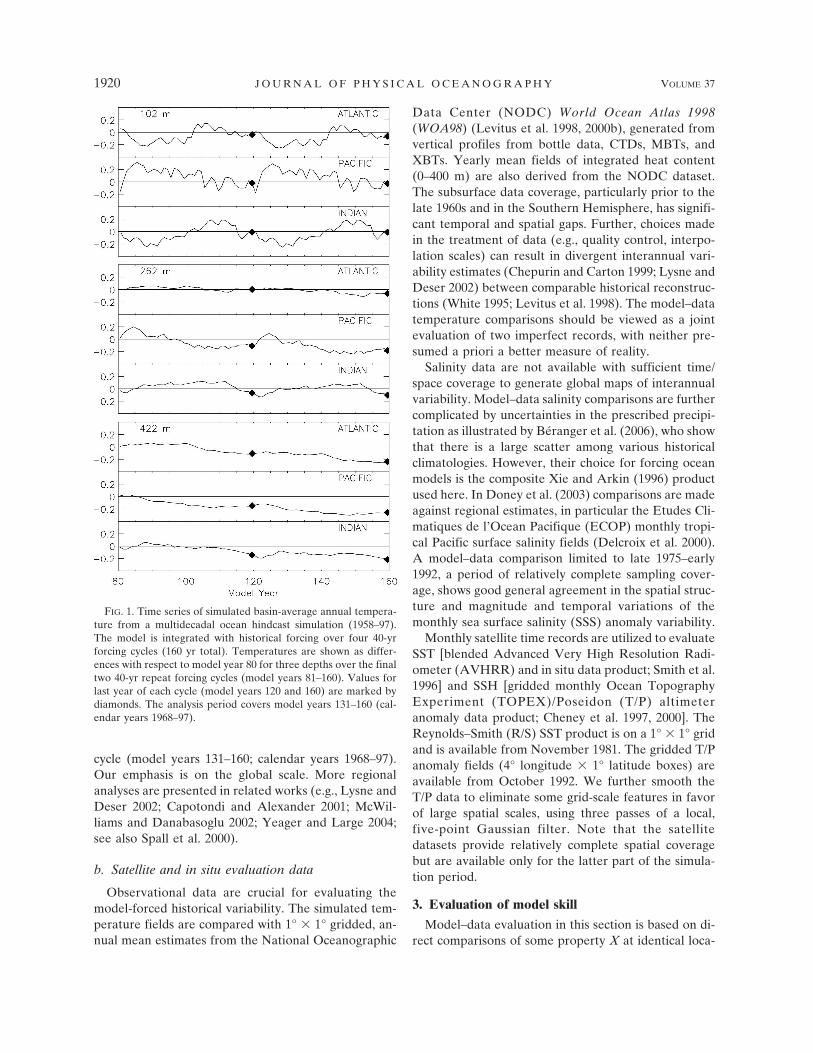
cycle (model years 131–160; calendar years 1968–97).Our emphasis is on the global scale. More regionalanalyses are presented in related works (e.g., Lysne andDeser 2002; Capotondi and Alexander 2001; McWil-liams and Danabasoglu 2002; Yeager and Large 2004;see also Spall et al. 2000).

b. Satellite and in situ evaluation data

Observational data are crucial for evaluating themodel-forced historical variability. The simulated tem-perature fields are compared with 1° � 1° gridded, an-nual mean estimates from the National Oceanographic

Data Center (NODC) World Ocean Atlas 1998(WOA98) (Levitus et al. 1998, 2000b), generated fromvertical profiles from bottle data, CTDs, MBTs, andXBTs. Yearly mean fields of integrated heat content(0–400 m) are also derived from the NODC dataset.The subsurface data coverage, particularly prior to thelate 1960s and in the Southern Hemisphere, has signifi-cant temporal and spatial gaps. Further, choices madein the treatment of data (e.g., quality control, interpo-lation scales) can result in divergent interannual vari-ability estimates (Chepurin and Carton 1999; Lysne andDeser 2002) between comparable historical reconstruc-tions (White 1995; Levitus et al. 1998). The model–datatemperature comparisons should be viewed as a jointevaluation of two imperfect records, with neither pre-sumed a priori a better measure of reality.

Salinity data are not available with sufficient time/space coverage to generate global maps of interannualvariability. Model–data salinity comparisons are furthercomplicated by uncertainties in the prescribed precipi-tation as illustrated by Béranger et al. (2006), who showthat there is a large scatter among various historicalclimatologies. However, their choice for forcing oceanmodels is the composite Xie and Arkin (1996) productused here. In Doney et al. (2003) comparisons are madeagainst regional estimates, in particular the Etudes Cli-matiques de l’Ocean Pacifique (ECOP) monthly tropi-cal Pacific surface salinity fields (Delcroix et al. 2000).A model–data comparison limited to late 1975–early1992, a period of relatively complete sampling cover-age, shows good general agreement in the spatial struc-ture and magnitude and temporal variations of themonthly sea surface salinity (SSS) anomaly variability.

Monthly satellite time records are utilized to evaluateSST [blended Advanced Very High Resolution Radi-ometer (AVHRR) and in situ data product; Smith et al.1996] and SSH [gridded monthly Ocean TopographyExperiment (TOPEX)/Poseidon (T/P) altimeteranomaly data product; Cheney et al. 1997, 2000]. TheReynolds–Smith (R/S) SST product is on a 1° � 1° gridand is available from November 1981. The gridded T/Panomaly fields (4° longitude � 1° latitude boxes) areavailable from October 1992. We further smooth theT/P data to eliminate some grid-scale features in favorof large spatial scales, using three passes of a local,five-point Gaussian filter. Note that the satellitedatasets provide relatively complete spatial coveragebut are available only for the latter part of the simula-tion period.

3. Evaluation of model skill

Model–data evaluation in this section is based on di-rect comparisons of some property X at identical loca-

FIG. 1. Time series of simulated basin-average annual tempera-ture from a multidecadal ocean hindcast simulation (1958–97).The model is integrated with historical forcing over four 40-yrforcing cycles (160 yr total). Temperatures are shown as differ-ences with respect to model year 80 for three depths over the finaltwo 40-yr repeat forcing cycles (model years 81–160). Values forlast year of each cycle (model years 120 and 160) are marked bydiamonds. The analysis period covers model years 131–160 (cal-endar years 1968–97).


tion and time in the observations and hindcast; that is,Xmodel(x, y, t) versus Xobs(x, y, t). When observationalsampling is sufficiently dense and spatially extensive,empirical orthogonal functions (EOFs) and their prin-cipal component (PCs) time series are preferred to dis-play concisely the most important spatial and temporalvariability in the model and observations. The PC timeseries are normalized to have a variance of 1.0, and theprojection of the original data onto an EOF at anyparticular point in time is recovered by PC(t) � EOF(x,y). When the observational coverage is not uniform,with large regions/times with poor sampling, we insteadmap the spatial patterns of rms variability and the localpoint cross correlation of the model and observationsover time.

One measure of model skill is whether the correla-tion between the model and observed variability is sta-tistically significant; that is, is the absolute value of thelinear correlation coefficient |r | greater than that ex-pected statistically for two uncorrelated, random vari-ables. We evaluate the statistical significance of r forthe PC time series, EOF spatial patterns, and localpoint temporal cross correlations using a two-tailed testat a significance level of 0.05 (95% confidence level)(Bevington and Robinson 2003). For example, thethreshold value is |rcrit | � 0.361 for a comparison of 30yr of model and data annual means (1968–97). We alsoassess the impact of the reduction in the effective de-grees of freedom in the linear correlation analysis dueto low-frequency variability (i.e., time/space autocorre-lation) (Emery and Thomson 2004).

The analyses utilize monthly mean properties X,from which we compute annual means X, long-termmeans �X �, and mean annual cycles Xa (i.e., mean Janu-ary, mean February, etc.). Various anomalies are thenformed:

X� � X � �X�,

X� � X � �X�, and

X* � X � Xa, �1

where X are the annual mean anomalies, X� are themonthly anomalies, and X* are the monthly deseason-alized anomalies. To exclude some particularly datasparse years and transients resulting from cycling backfrom 1997 to 1958 forcing, we focus solely on the the30-yr span 1968–97.

a. Sea surface height

With the availability of nearly global coverage fromsatellite altimeters, SSH variability provides a usefulmetric for evaluating the hindcast. On scales larger than

the mesoscale (�500 km), the dominant factors con-tributing to intraseasonal and interannual SSH varia-tions include barotropic and baroclinic adjustments tosurface wind stress variations and steric anomalies dueto heat and freshwater surface fluxes and lateral heatand freshwater convergence.

A main focus here is on the SSH signatures gener-ated by interannual variability in upper-ocean tempera-ture or equivalently heat content. Because seawater ex-pands as it warms, a positive monthly deseasonalizedtemperature anomaly T* results in a positive SSHanomaly �*:

�* � �0

�z0

�T* dz, �2

where is the thermal expansion coefficient, and z0 isan appropriate upper-ocean depth scale. For an ap-propriate to the tropical and midlatitude upper ther-mocline (T � 15°C), a uniform 0.1°C anomaly over theupper 400 m leads to an �* � l cm; as drops sharplywith temperature, the steric SSH anomaly for the sametemperature anomaly at polar latitude would be 3–4times smaller. A similar calculation could be done toestimate the generally smaller effect of freshwater (sa-linity) anomalies on �* using �S*.

To reduce the data size for the EOF analysis, themodel SSH is binned in boxes 7.2° in longitude, varyingbetween 1.2° and 2.4° in latitude. The monthly T/P SSHis binned in latitude using 2° boxes. The first two EOFs,accounting for about one-half of the respective vari-ances (47% for T/P and 55% for model), are presentedin Fig. 2 together with the principal component timeseries. The majority of the monthly rms variability inthe model deseasonalized SSH signal from the modelarises because of dynamic adjustments to surface windforcing and resulting advective redistribution of upper-ocean heat and salt content, consistent with previousfindings (e.g., Stammer 1997; Fu 2003).

The hindcast simulation reproduces well the domi-nant space/time patterns of SSH variability seen in theT/P data, particularly in the Tropics. The agreement ofprincipal component time series is quite encouraging,with temporal model–data correlations of 0.99 and 0.98for EOF1 and EOF2, respectively. EOF1 is well sepa-rated from EOF2 and is associated with ENSO vari-ability. The onset and evolution of the 1997 ENSOevent is clearly depicted in the EOF1 principal compo-nent time series. The second EOF is weaker and con-centrated in the Indian Ocean, with a stronger exten-sion into tropical South Pacific in the observations thanin the model; EOF2 is sometimes referred to as theIndian Ocean zonal mode (e.g., Saji et al. 1999; Yu and

JULY 2007 D O N E Y E T A L . 1921

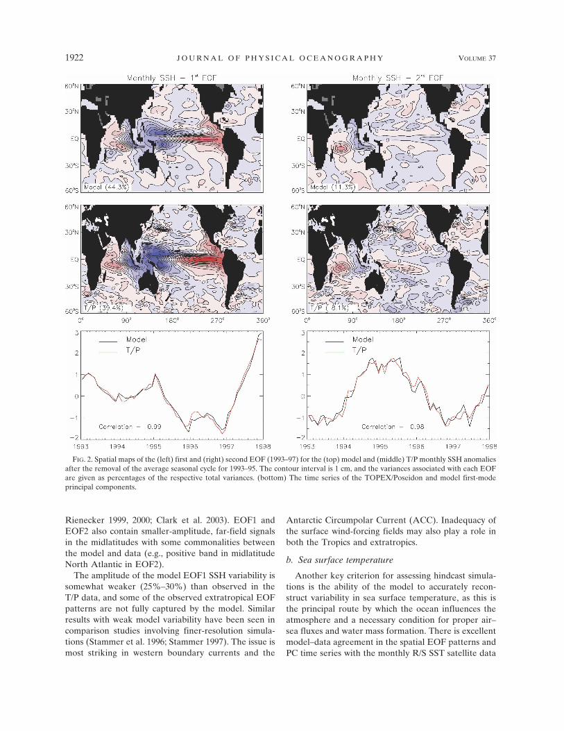
Rienecker 1999, 2000; Clark et al. 2003). EOF1 andEOF2 also contain smaller-amplitude, far-field signalsin the midlatitudes with some commonalities betweenthe model and data (e.g., positive band in midlatitudeNorth Atlantic in EOF2).

The amplitude of the model EOF1 SSH variability issomewhat weaker (25%–30%) than observed in theT/P data, and some of the observed extratropical EOFpatterns are not fully captured by the model. Similarresults with weak model variability have been seen incomparison studies involving finer-resolution simula-tions (Stammer et al. 1996; Stammer 1997). The issue ismost striking in western boundary currents and the

Antarctic Circumpolar Current (ACC). Inadequacy ofthe surface wind-forcing fields may also play a role inboth the Tropics and extratropics.

b. Sea surface temperature

Another key criterion for assessing hindcast simula-tions is the ability of the model to accurately recon-struct variability in sea surface temperature, as this isthe principal route by which the ocean influences theatmosphere and a necessary condition for proper air–sea fluxes and water mass formation. There is excellentmodel–data agreement in the spatial EOF patterns andPC time series with the monthly R/S SST satellite data

FIG. 2. Spatial maps of the (left) first and (right) second EOF (1993–97) for the (top) model and (middle) T/P monthly SSH anomaliesafter the removal of the average seasonal cycle for 1993–95. The contour interval is 1 cm, and the variances associated with each EOFare given as percentages of the respective total variances. (bottom) The time series of the TOPEX/Poseidon and model first-modeprincipal components.


Fig 2 live 4/C

product (1982–97) (Fig. 3). The first SST EOF captures20%–25% of the total variance and displays the classicENSO pattern, with anomalies in the eastern tropicalPacific and along the North American west coast out ofphase with those in the western tropical Pacific andsubtropical gyres (Neelin et al. 1998). The second EOF(6%–8% of total variance) projects more into the tem-perate and subpolar North Pacific and North Atlantic.Quantitative measures of model skill are high with spa-tial and temporal correlations of 0.96 and 0.98 (EOF1)and 0.84 and 0.89 (EOF2). Similar spatial variabilitypatterns and model–data agreement are found for an-nual mean SST anomalies from the model and the in

situ WOA98 data for the full analysis time period(1968–97; Doney et al. 2003).

The model skill in replicating observed SST interan-nual variability could, in theory, represent compensat-ing errors in model physics and surface heat fluxes. Forocean models forced by a prescribed atmospheric state,the atmosphere has a large effective heat capacity, andthe ocean SST will, perhaps incorrectly, closely trackthe prescribed air temperature (e.g., Seager et al. 1995).To examine this issue, we include here a short diversioninto the mechanisms underlying interannual SST vari-ability. Figure 4 displays the correlation coefficient ateach model grid point between the annual average heat

FIG. 3. Spatial maps of the (left) first and (right) second EOF mode for the (top) model and (middle) R/S monthly SST anomalies(1982–97) after removal of the average seasonal cycle. The spatial pattern correlation is 0.96. The contour interval is 0.2°C, and thevariances associated with each EOF are given as percentages of the respective total variances. (bottom) The time series of theReynolds–Smith (red) and model (black) first-mode principal components.

JULY 2007 D O N E Y E T A L . 1923

Fig 3 live 4/C

flux anomaly and change in SST for the correspondingyear. The “observational” fluxes are obtained by simplyreplacing the model SST with R/S SST in the bulk forc-ing procedure. The spatial patterns in the model andobservation correlation maps are similar but with lowercorrelation values in the observations, perhaps due tomeasurement error and data sparseness in either the

SSTs or atmospheric forcing and because in the modelsurface fluxes do not alter the air temperature and hu-midity as they do in nature.

High positive correlations, such as in the subtropics,indicate regions where interannual SST variabilitycould result largely from the specified atmosphericforcing. At midlatitudes the correlation tends to be

FIG. 4. Spatial distributions of the local correlation coefficient at each grid point between theannual average heat flux and change in SST over the corresponding year from the (top)observation record and the (bottom) model hindcast.


Fig 4 live 4/C

lower, suggesting at least some role for ocean processes,for example, variability in the effective depth to whichsurface fluxes are mixed or lateral circulation. Negativecorrelations occur at high latitudes where sea ice pro-cesses appear to play a dominant role; colder SSTs areindicative of ice formation, which tends to reduce air–sea heat loss leading to negative correlation. There arealso significant regions of high negative correlationalong the equator of both the Atlantic and Pacific ba-sins. The negative correlation arises when the oceansurface is cooling despite anomalous surface flux warm-ing, or the reverse. This can only occur if internal oceanprocesses are generating the SST changes. The surfaceheat flux anomalies are then likely a response, in part,to the SST anomalies, and in terms of the upper-oceanheat budget are acting to damp the ocean-driven vari-ability, cooling warm anomalies and heating cold ones.

To demonstrate, consider the thermal budget for thetropical Pacific, shown in more detail in Fig. 5 as a timeseries of the first EOF principal components for themodel and diagnosed net surface heat fluxes (upperpanel) and the model net surface heat flux and tempo-ral derivative of model SST (lower panel). The similar-ity of the model and diagnosed net heat flux EOFs,indicative of ENSO variability, is marked by high spa-

tial pattern (0.73: Doney et al. 2003) and temporal(0.79) correlations over the eastern tropical Pacific. Thetemporal heat flux correlation is somewhat lower thanthat for the first SST EOF (0.98; Fig. 3, left panels)because of nonlinearities in the heat flux calculationand the different spatial domains. The | r |crit valuewould be 0.14 for the temporal correlation with N �192 samples if the individual months were independent.In actuality, the effective degrees of freedom are closerto �16 due to the temporal autocorrelation of about ayear; this leads to a revised |r |crit � 0.47, which is stillgreatly below the observed value of 0.79. A similar ex-ercise for the spatial EOF patterns comes to the samebasic conclusion, balancing the large number of gridpoints with the reduction in degrees of freedom due tothe spatial correlation scales (500–5000 km dependingon meridional or zonal direction).

If SST in the model was simply being driven by netsurface heat fluxes, one would expect a positive corre-lation near 1 for �SST/�t and qnet; in fact, the correlationfor the tropical Pacific is essentially zero (0.004). Thewarming associated with the ENSO events of 1982–83,1986–87, 1991–92, and 1997–98 is accompanied by nega-tive (cooling) net heat flux, as indicated by the shadingin Fig. 5. There are also significant regions of high nega-

FIG. 5. Time series of the first EOF principal components (1982–97) for the thermal budgetfor the tropical Pacific (from 10°S to 10°N east of 150°E). (top) The model (solid) anddiagnosed (dashed) net surface heat flux qnet EOFs, where the diagnosed fluxes are computedusing the R/S SST and the same atmospheric forcing as the model simulations. (bottom) Thefirst EOFs for model net surface heat flux (solid) and the temporal derivative of the modelSST, �SST/�t (dashed). Shading denotes periods when the model temporal derivative is op-posite in sign to the net heat flux.

JULY 2007 D O N E Y E T A L . 1925

tive correlation along the equator of both the Atlanticand Pacific basins. The out-of-phase SST–heat flux re-lationship shows that the model net heat flux anomaliesare mostly a response to increasing SST (not the re-verse) and that the model SST signal (and thus model–data skill) reflects success in replicating the oceanicphysics.

c. Heat content and subsurface temperature

We utilize integrated annual-mean heat contentanomalies from the surface to 400 m as a third evalua-tion metric for the hindcast. Heat content provides asingle, compact method for displaying upper-oceantemperature variability, and variability in upper-oceanheat content can be estimated with some confidencefrom observations over many parts of the ocean. Theannual mean heat content anomaly H is computedfrom

H� � �0

400

�cpT� dz, �3

where cp and � are the specific heat and density. Theuniform temperature anomaly of 0.1°C discussed abovefor scaling �* anomalies with representative cp and �values produces H � 0.16 GJ m�2; an anomaly of thissize would be generated by a net surface heat fluxanomaly of about 5 W m�2 applied over a full year.

The main spatial patterns of rms(H) (Fig. 6) arecomparable across the hindcast and WOA98 data, withmaxima in the tropical Indo–Pacific, western boundarycurrents, Southern Ocean, and subpolar North Atlan-tic. The spatial patterns of SST and heat content vari-ability differ considerably. In the Tropics, temperaturevariability shifts progressively westward and off equa-tor moving down the water column, decoupled from thesurface due to stratification. In the extratropics, tem-perature anomalies are more coherent in the verticalbecause of deep winter mixing and because the vari-ability in the location and strength of the westernboundary currents and the ACC tend to span the upperthermocline.

Relative to WOA98, the model heat content variabil-ity in the tropical Pacific is more localized into discrete,zonal off-equatorial bands (Lysne and Deser 2002).The hindcast also contains considerably weaker vari-ability in the Agulhas retroflection and Brazil–Malvinasconfluence, which almost certainly reflects the fact thatthe coarse-resolution model is still too viscous to cap-ture fully the dynamics in these regions. The modelvariability is lower than that in WOA98 along the Ant-arctic Circumpolar Current in the Southern Ocean, buthere the model–data differences likely are a combina-

tion of model and forcing errors together with inad-equate in situ sampling.

The model–data cross correlations for the local an-nual heat storage anomalies (Fig. 6, bottom panel) arelarge and significant (�0.6) in the North Pacific, tropi-cal Pacific, and northern North Atlantic. The compari-son shows essentially no relationship in the SouthernOcean and the Brazil–Malvinas confluence, where theobserved data coverage is more limited, and the fielddata provide poor estimates of heat content variability.Even specific features such as the sampling hole in thecentral and eastern tropical North Atlantic (Levitus etal. 1998; see also Fig. 2 in Doney et al. 2003) show updistinctly as minima in the cross-correlation field. AnEOF analysis for 1968–97 of the annual heat contentanomalies (not shown) highlights the same basicENSO-driven tropical spatial patterns as found for theSSH analysis.

FIG. 6. Spatial maps of the rms annual heat storage (integrated0–400 m) variability (1968–97) for the (top) model and (middle)observed WOA98 (Levitus et al. 1998) datasets and (bottom) thespatial map of the anomaly cross correlation.


Fig 6 live 4/C

4. Dynamics of interannual variability

We then use the model solutions to explore themechanisms generating the variability, focusing on in-terannual variability of the dominant upper-ocean heatbudget terms. For many ocean regions, subsurface ob-servations are too sparse to reconstruct historical varia-tions in the storage, ocean transport, and, to some ex-tent, even surface flux terms. The hindcast simulation,on the other hand, computes a dynamically consistent,closed heat budget for the global ocean from which wecan develop hypotheses testable against past and/or fu-ture observations on more regional scale.

a. Net annual heat storage anomalies

Over the course of a year, upper-ocean (400 m) heatcontent H changes by an amount �H, the net annualheat storage, due to the combined effect of the netsurface heat flux and the divergence of ocean heattransport. From the hindcast simulation, we compute�H over the depth interval 0–400 m (GJ m�2) (or ef-fectively the annual heat budget imbalance integratedover that depth range; see below) for each year at eachgrid point using monthly mean model output. Becausemodel temperature was stored as monthly means ratherthan as instantaneous values at the end of months, �His computed using H values averaged for December andthe following January. To remove the effects of anylong-term model drift, net annual heat storage anoma-lies �H are computed by subtracting ��H � [Eq. (1)].With this normalization, we also remove any net long-term, secular warming (Levitus et al. 2000a; Willis et al.2004). The annual heat content anomaly (section 3c) isapproximately the net integral over time of the past netannual heat storage anomalies, H � � �H dt, differ-ences arising from the different temporal averaging/analysis periods (cf. top panel, Fig. 7 with Fig. 6).

b. Partitioning heat budget variability bymechanism

We partition the contributions to the net annual heatstorage anomalies (GJ m�2) into specific physical com-ponents:

�H� � Q� � A� � E� � V� � R, �4

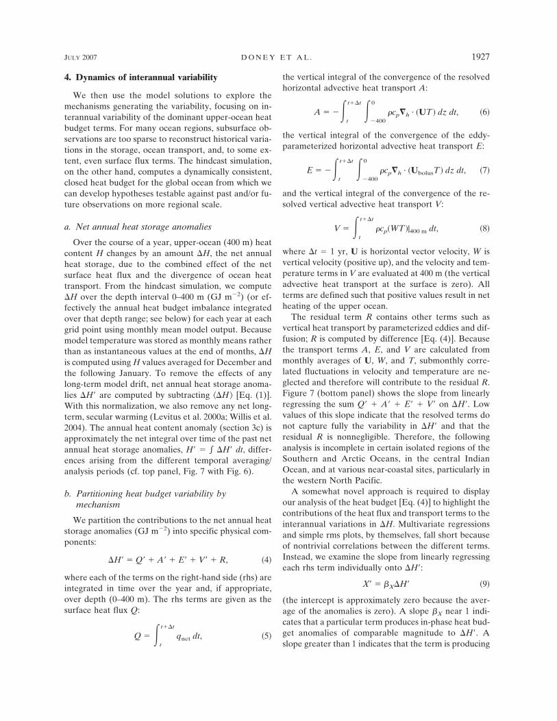
where each of the terms on the right-hand side (rhs) areintegrated in time over the year and, if appropriate,over depth (0–400 m). The rhs terms are given as thesurface heat flux Q:

Q � �t

t��t

qnet dt, �5

the vertical integral of the convergence of the resolvedhorizontal advective heat transport A:

A � ��t

t��t ��400

0

�cp�h · �UT dz dt, �6

the vertical integral of the convergence of the eddy-parameterized horizontal advective heat transport E:

E � ��t

t��t ��400

0

�cp�h · �UbolusT dz dt, �7

and the vertical integral of the convergence of the re-solved vertical advective heat transport V:

V � �t

t��t

�cp�WT |400 m dt, �8

where �t � 1 yr, U is horizontal vector velocity, W isvertical velocity (positive up), and the velocity and tem-perature terms in V are evaluated at 400 m (the verticaladvective heat transport at the surface is zero). Allterms are defined such that positive values result in netheating of the upper ocean.

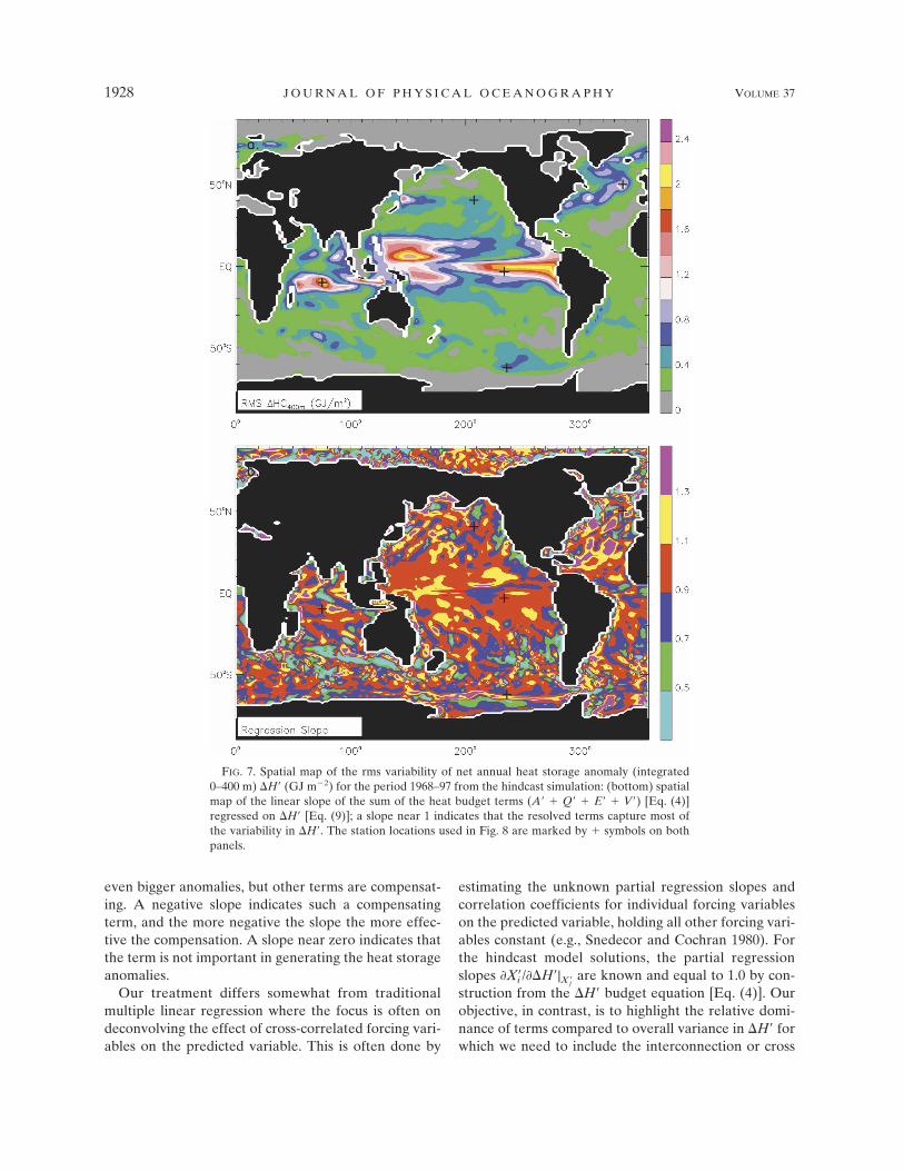
The residual term R contains other terms such asvertical heat transport by parameterized eddies and dif-fusion; R is computed by difference [Eq. (4)]. Becausethe transport terms A, E, and V are calculated frommonthly averages of U, W, and T, submonthly corre-lated fluctuations in velocity and temperature are ne-glected and therefore will contribute to the residual R.Figure 7 (bottom panel) shows the slope from linearlyregressing the sum Q � A � E � V on �H. Lowvalues of this slope indicate that the resolved terms donot capture fully the variability in �H and that theresidual R is nonnegligible. Therefore, the followinganalysis is incomplete in certain isolated regions of theSouthern and Arctic Oceans, in the central IndianOcean, and at various near-coastal sites, particularly inthe western North Pacific.

A somewhat novel approach is required to displayour analysis of the heat budget [Eq. (4)] to highlight thecontributions of the heat flux and transport terms to theinterannual variations in �H. Multivariate regressionsand simple rms plots, by themselves, fall short becauseof nontrivial correlations between the different terms.Instead, we examine the slope from linearly regressingeach rhs term individually onto �H:

X� � �X�H� �9

(the intercept is approximately zero because the aver-age of the anomalies is zero). A slope �X near 1 indi-cates that a particular term produces in-phase heat bud-get anomalies of comparable magnitude to �H. Aslope greater than 1 indicates that the term is producing

JULY 2007 D O N E Y E T A L . 1927

even bigger anomalies, but other terms are compensat-ing. A negative slope indicates such a compensatingterm, and the more negative the slope the more effec-tive the compensation. A slope near zero indicates thatthe term is not important in generating the heat storageanomalies.

Our treatment differs somewhat from traditionalmultiple linear regression where the focus is often ondeconvolving the effect of cross-correlated forcing vari-ables on the predicted variable. This is often done by

estimating the unknown partial regression slopes andcorrelation coefficients for individual forcing variableson the predicted variable, holding all other forcing vari-ables constant (e.g., Snedecor and Cochran 1980). Forthe hindcast model solutions, the partial regressionslopes �Xi /��H|Xj

are known and equal to 1.0 by con-struction from the �H budget equation [Eq. (4)]. Ourobjective, in contrast, is to highlight the relative domi-nance of terms compared to overall variance in �H forwhich we need to include the interconnection or cross

FIG. 7. Spatial map of the rms variability of net annual heat storage anomaly (integrated0–400 m) �H (GJ m�2) for the period 1968–97 from the hindcast simulation: (bottom) spatialmap of the linear slope of the sum of the heat budget terms (A � Q � E � V) [Eq. (4)]regressed on �H [Eq. (9)]; a slope near 1 indicates that the resolved terms capture most ofthe variability in �H. The station locations used in Fig. 8 are marked by � symbols on bothpanels.


Fig 7 live 4/C

correlation among the different budget terms. The re-gression slopes �X [Eq. (9)] reflect this and differ from1.0 either because the variance of variable Xi is sub-stantially smaller than other forcing terms or becauseXi is out of phase or anticorrelated with more dominantterms. Further, the model regression slopes can be usedwith observed ocean heat content anomalies to givediagnoses typically unknown and difficult to measureprocesses.

Time series for �H and corresponding local budgetterms from Eq. (4) are shown in Fig. 8 for five locationswhere rms(�H) is relatively high (marked by plus signsin Figs. 7, 9, and 10). The primary driver for interannualvariability is A (green), especially in the Tropics; V(magenta) is the next most significant term in the bud-get and tends to be anticorrelated to �H. These pat-terns are well defined in the scatterplots from the tropi-cal Pacific (Fig. 8, top panel) and Indian (Fig. 8, secondpanel from top) Oceans (right column) where the slopeof A on �H is greater than 1, the slope of V on �His smaller and less than 0, and the small scatter aboutstraight lines indicates that the forcing terms are highlycorrelated with the net heat storage response. The op-posing signals in A and V reflect the fact that thehorizontal and vertical components are partiallycoupled due to mass conservation; the regression slopeof their sum (not shown) on �H is positive and close to1.0, indicating the dominance of advection.

At extratropical sites A remains positive, but �Hevolution is often governed by a mix of forcing terms.The net heat flux term Q (dark blue) contributes tointerannual net heat storage anomalies while the eddy-parameterized transport term E (light blue) evolves onlonger, multiyear scales. The linear correlations for in-dividual terms tend to be lower than in the Tropics(more scatter about the regression lines). At the South-ern Ocean site (Fig. 8, second panel from bottom), Qis as significant as A, although the variance in �H atthis location is much lower than in the Tropics. At atemperate North Atlantic site (bottom panel), the bal-ance of terms is time dependent. Whereas A driveslarge �H variations in the 1980s, significant E anoma-lies in the early 1970s and 1990s damp the effects of theresolved heat transport, resulting in lower �H duringthese periods. The inclusion of only four rhs terms(Q, A, E, and V) in the heat budget analysis is cer-tainly justified at the tropical locations (top two pan-els), as the sum of the four (red line) is very nearlyequal to the storage anomaly (black line). The exclu-sion of other budget terms introduces somewhat largerdiscrepancies in the extratropics (Fig. 8, bottom threepanels).

Figure 9 displays global spatial maps of the regres-

sion slopes of the four rhs physical terms regressed on�H. The maps are masked (gray) in regions whererms(�H) is small and/or the regression slope is statis-tically insignificant. In those regions of the Tropics andNorthern Hemisphere extratropics where rms(�H)(Fig. 7) is substantial, A dominates (slopes of 0.8–1.2),is often partially compensated by other terms (slope�1.2; mostly V), and is strongly correlated with �H(not shown). The A regression slope decreases (0.3 ��A � 0.8) in the Southern Ocean, where other termsgrow in importance. The slope of the resolved verticaladvective heat convergence V regressed on �H slopeis negative for most of the global ocean, with largeregions in the subtropics with values between �0.8 and�0.3 (and in some locations �1.2 � �V � �0.8).

The Q regression slope is small and often slightlynegative in the Tropics, damping net heat storage vari-ability. Local heat fluxes play a larger, more statisticallysignificant, and positive forcing role in the extratropics(regression slopes of 0.3–0.8). Note, however, that largeQ regression slopes tend to occur in areas whererms(�H) is relatively weak; for example, in the NorthAtlantic and most of the Southern Ocean, the bands oflarge Q regression slope surround, but do not include,the rms(�H) maxima along the track of the GulfStream/North Atlantic current and ACC. An exceptionis the region near �60°S in the Pacific sector of theSouthern Ocean included as one of the locations in(Fig. 8). The eddy-parameterized term E plays a minorrole in interannual thermal variability except for a fewlocalized spots along the equator in the Indo–Pacificbasins, Southern Ocean, subpolar North Atlantic, andArctic. In summary, the partitioning of the heat budgetshows that anomalies in the convergence of the advec-tive heat transport (A and V) dominate net annualheat storage variability in the well-stratified Tropicsand subtropics; at mid- to high latitudes, local anoma-lies in air–sea heat flux Q also play a significant role.

c. Decomposing mean and time-varying velocityand temperature components

The A term [Eq. (6)] can be decomposed based onthe mean and time-varying components of velocity andtemperature:

A� � ��t

t��t ��400

0

�cp�h · ��U�T � � U��T�

� �U*T*�� dz dt. �10

The three terms on the rhs represent, respectively, theannual net heat storage anomaly due to the conver-gence of the mean velocity acting on temperatureanomalies, velocity anomalies acting on mean tempera-

JULY 2007 D O N E Y E T A L . 1929

FIG. 8. Time series of model upper-ocean heat budgets for five model locations with large rmsvariability in net annual heat storage anomaly, rms(�H) (see Fig. 7): (from top to bottom) easterntropical Pacific; tropical Indian; northern central Pacific; Southern Ocean; and subpolar North Atlantic.(left) Time series of the annual change in net heat storage anomaly (integrated 0–400 m) �H (blackwith � symbols) together with the annual heat budget anomalies [Eq. (4)]: surface heat flux Q (blue);convergence of resolved A (green) and eddy-parameterized E (cyan) horizontal advective heat trans-port; and convergence of the resolved vertical advective heat convergence V (magenta). The sum of thefour rhs terms is shown in red. (right) Display of x–y scatterplots of the individual budget terms ( y axis)vs �H (x axis); all variables: GJ m�2.


Fig 8 live 4/C

ture, and the correlation arising from monthly desea-sonalized velocity and temperature anomalies, U* andT* [Eq. (1)]. The third term is generally small (Jayneand Marotzke 2001, 2002) and will be neglected. In asimilar fashion as in Fig. 9, the remaining two terms areregressed on A (Fig. 10).

Over much of the model ocean, A is dominated by�h · U�T � (Fig. 10). The �h · �U�T term becomes im-portant in the south equatorial Indian Ocean, westernNorth Atlantic, and ACC where the mean advectivecurrents are moderate to strong. Note the regions ofstrong negative �h · �U�T regression slope (�0.8 � � ��0.3) in the ACC and Gulf Stream, indicating that ve-locity anomalies and temperature anomalies are work-ing against each other. Correlated U and T anomalies

arise due to changes in current strength and lateralshifts in current location.

The vertical term V can be decomposed in a similarmanner:

V� � �t

t��t

�cp��W�T � � W��T� � �W*T*�� dt. �11

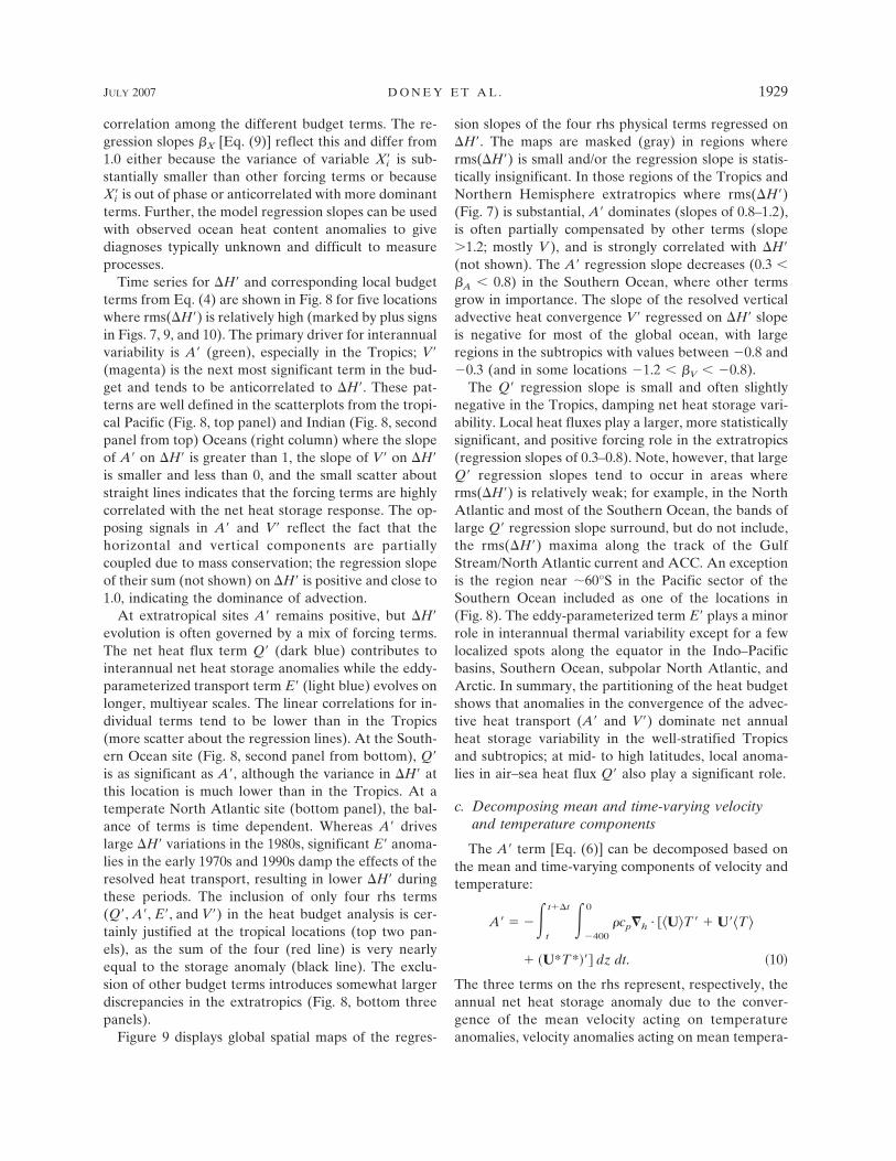
As with horizontal convergence, V is dominated byW�T � (not shown). Indeed, the spatial patterns ofrms(W) at the base of the analysis domain (396 m)(bottom left panel of Fig. 11) match well those of theoff-equator tropical rms(�H) variability (Fig. 7).

To examine the degree to which vertical velocityvariability rms(W) is related to anomalies in local windforcing, we compare W with the anomalies in vertical

FIG. 9. Spatial maps displaying linear slope of heat budget anomaly terms regressed on hindcast net annual heat storageanomaly �H [Eq. (4)]: (top left) the convergence of resolved horizontal advective heat transport A; (top right) surfacenet heat flux Q; (bottom left) convergence of vertical advective heat transport V; and (bottom right) convergence ofeddy-parameterized horizontal advective heat transport E. A slope near 1 indicates a dominant forcing term. A slopegreater than 1 indicates that the term is producing even bigger anomalies, but other terms are compensating. A negativeslope indicates such a compensating term, and the more negative the slope the more effective the compensation. A slopenear zero indicates that the term is not important in generating the heat budget anomalies. The maps are grayed out inregions where the regression correlation is not significant at the 95% level and where rms(�H) � 0.16 GJ m�2 (Fig. 7).

JULY 2007 D O N E Y E T A L . 1931

Fig 9 live 4/C

Ekman velocity WEk computed from the curl of thewind stress (Fig. 11). We concentrate on two depths, theapproximate base of the surface wind-driven layer (50m) and the base of the analysis domain (396 m). Theright column of Fig. 11 displays spatial maps of theregression slope of WEk on W; WEk is not computedright on the equator because f, the Coriolis parameter,vanishes. Not surprisingly local wind forcing and Ek-man pumping generally dominate in the upper watercolumn (50 m). The regression slopes are typically0.8 � � � 1.2 with large regions of the Southern Hemi-sphere Tropics where � � 1.2, suggesting some cancel-lation by other terms. Interestingly, the slopes are oftensomewhat lower (0.3 � � � 0.8) in the Northern Hemi-sphere Tropics. Deeper in the water column remoteforcing plays a stronger role, especially in the Tropicsand subtropics, western boundary currents, and parts ofthe ACC. Furthermore, the advective heat transportvariability in the Tropics and subtropics mostly reflectsvelocity anomalies times the mean temperature fieldwhile variability in mid- to high latitudes arises fromboth velocity and temperature anomalies.

d. Heave and spice analysis of T and S anomalies

The vertically integrated heat budget analysis of �Hconceals the considerable vertical structure of the in-terannual tracer anomalies in the upper 400 m. Aver-aged over basin to global scales, the subsurface inter-annual rms(T) in the hindcast and observations peaksat about 0.45°C between 50 and 150 m before decliningwith depth to about 0.15°C by 400 m (not shown; see

Doney et al. 2003). The magnitude of model rms(T ) isabout 25% lower than that in the WOA98 observa-tional data. Globally, model rms(S) peaks shallower inthe water column (50–100 m) at about 0.06 psu. Salinityobservations are limited, especially at depth, so thehindcast provides a view to interannual subsurface sa-linity variability.

The simulated subsurface temperature and salinityfields often vary in phase, indicating a common under-lying mechanism. To explore this behavior, we partitionthe subsurface temperature and salinity variability at agiven location and depth into two terms: changes in thewater mass characteristics on surfaces of constant den-sity (spice) and changes due to vertical displacement ofisopycnal surfaces (heave). Both vertical and lateralprocesses could contribute to the heaving of isopycnalsat a given location. Similarly, a spice anomaly couldarise through either lateral advection along an isopyc-nal or through vertical diapycnal mixing across anisopycnal (Yeager and Large 2004). The derivation out-lined below differs somewhat from other methods pro-posed in the literature (e.g., Bindoff and McDougall1994), but the overall objective is similar.

The analysis starts with the annual mean tracer val-ues X, long-term means �X�, and anomalies X com-puted for both T and S at each model grid cell for yeary on fixed depth surfaces z. The spice anomaly for agiven year is defined then as the difference between theannual mean tracer value and the long-term mean ofthe tracer �X��(y) on the isopycnal �(y) found at depthz in year y:

FIG. 10. Spatial maps displaying the decomposition of the convergence of the resolved horizontal advective heattransport anomaly A [Eq. (10)] based on the mean and time-varying components of velocity and temperature. Each panelshows the linear slope of the individual terms regressed on A: (left) heat convergence anomalies due to velocity anomaliestimes mean temperature U��T � and (right) mean velocity time temperature anomalies �U�T. The maps are grayed out inregions where the regression correlation is not significant at the 95% level and where rms(�H) � 0.16 GJ m�2 (Fig. 7).


Fig 10 live 4/C

X�S � X � �X�� y. �12

Because the density field evolves in time, �(y) and�X ��(y) also vary with time and are computed separatelyfor each individual year. The heave component of thetracer anomaly is defined as the difference between theclimatological mean of the tracer on the isopycnal sur-face and on the fixed depth surface:

X�H � �X��y � �X�z. �13

By construction, the annual mean tracer anomaly is thesum of the spice and heave anomalies:

X� � X�S � X�H. �14

In the special case where water mass characteristicson isopycnal surfaces remain constant in time andtracer anomalies are due solely to vertical isopyc-nal displacement, then T S � SS � 0, T � T H, and S �

SH (pure heave). In the opposite extreme of no verti-cal displacement of isopycnal surfaces, �(y) � ��z,�X ��(y) � �X�z, and T � T S, S � SS (pure spice). Ingeneral, both XS and XH are nonzero, with the firstterm reflecting processes creating tracer anomalies onthe �(y) isopycnal and the second term associated withisopycnal displacements.

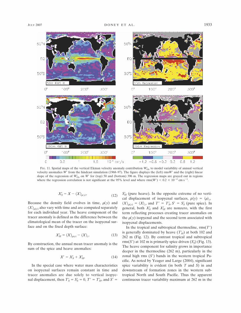
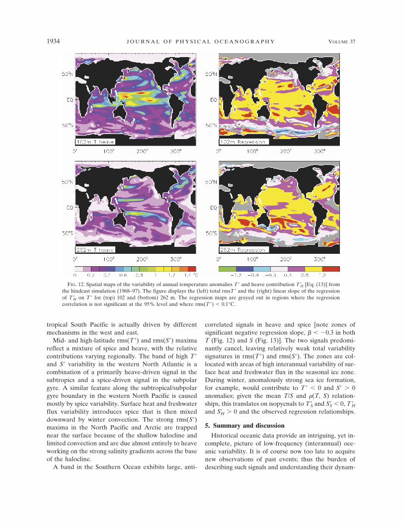
In the tropical and subtropical thermocline, rms(T )is generally dominated by heave (T H) at both 102 and262 m (Fig. 12). By contrast tropical and subtropicalrms(S) at 102 m is primarily spice driven (SS) (Fig. 13).The heave component for salinity grows in importancedeeper in the thermocline (262 m), particularly in thezonal high rms (S) bands in the western tropical Pa-cific. As noted by Yeager and Large (2004), significantspice variability is evident (in both T and S) in anddownstream of formation zones in the western sub-tropical North and South Pacific. Thus the apparentcontinuous tracer variability maximum at 262 m in the

FIG. 11. Spatial maps of the vertical Ekman velocity anomaly contribution WEk to model variability of annual verticalvelocity anomalies W from the hindcast simulation (1968–97). The figure displays the (left) rmsW and the (right) linearslope of the regression of WEk on W for (top) 50 and (bottom) 396 m. The regression maps are grayed out in regionswhere the regression correlation is not significant at the 95% level and where rms(W) � 0.2 � 10�4 cm s�1.

JULY 2007 D O N E Y E T A L . 1933

Fig 11 live 4/C

tropical South Pacific is actually driven by differentmechanisms in the west and east.

Mid- and high-latitude rms(T ) and rms(S) maximareflect a mixture of spice and heave, with the relativecontributions varying regionally. The band of high T and S variability in the western North Atlantic is acombination of a primarily heave-driven signal in thesubtropics and a spice-driven signal in the subpolargyre. A similar feature along the subtropical/subpolargyre boundary in the western North Pacific is causedmostly by spice variability. Surface heat and freshwaterflux variability introduces spice that is then mixeddownward by winter convection. The strong rms(S)maxima in the North Pacific and Arctic are trappednear the surface because of the shallow halocline andlimited convection and are due almost entirely to heaveworking on the strong salinity gradients across the baseof the halocline.

A band in the Southern Ocean exhibits large, anti-

correlated signals in heave and spice [note zones ofsignificant negative regression slope, � � �0.3 in bothT (Fig. 12) and S (Fig. 13)]. The two signals predomi-nantly cancel, leaving relatively weak total variabilitysignatures in rms(T ) and rms(S). The zones are col-located with areas of high interannual variability of sur-face heat and freshwater flux in the seasonal ice zone.During winter, anomalously strong sea ice formation,for example, would contribute to T � 0 and S � 0anomalies; given the mean T/S and �(T, S) relation-ships, this translates on isopycnals to T S and SS � 0, T Hand SH � 0 and the observed regression relationships.

5. Summary and discussion

Historical oceanic data provide an intriguing, yet in-complete, picture of low-frequency (interannual) oce-anic variability. It is of course now too late to acquirenew observations of past events; thus the burden ofdescribing such signals and understanding their dynam-

FIG. 12. Spatial maps of the variability of annual temperature anomalies T and heave contribution T H [Eq. (13)] fromthe hindcast simulation (1968–97). The figure displays the (left) total rmsT and the (right) linear slope of the regressionof T H on T for (top) 102 and (bottom) 262 m. The regression maps are grayed out in regions where the regressioncorrelation is not significant at the 95% level and where rms(T ) � 0.1°C.


Fig 12 live 4/C

ics falls jointly on data synthesis and modeling studies,with data assimilation playing an increasingly signifi-cant role. We demonstrate that a significant fraction ofthe observed low-frequency signal in upper-ocean tem-perature can be captured in an unconstrained simula-tion forced with atmospheric reanalysis and satellitedata.

The model–data agreement is encouraging becauseneither the ocean model nor the atmospheric forcingwere specifically tuned to improve the skill of the in-terannual simulations, though significant efforts havebeen invested to improve the underlying simulatedmean ocean state (Large et al. 1997; Gent et al. 1998).This suggests that numerical simulation of many basicaspects of the observed large-scale ocean variability isrobust to particular details of the formulation of themodel and surface forcing.

Satellite data records (SST, SSH), apart from beingconfined to the surface and of limited duration, serve as

excellent comparative datasets because of the relativelyfrequent global coverage. Model agreement with thesedata is generally very good in both magnitude andphase of interannual variability, with the exception ofthe weak midlatitude SSH variability. The model com-parison with in situ (WOA98) SST variability is alsofavorable. Not surprisingly, large model–data differ-ences emerge in regions of sparse sampling, and inmany regions the model simulations may provide theonly viable, historical estimate of oceanic variability.

Our hindcast simulation is conducted in fully prog-nostic mode, reserving the oceanic observationaldatasets as independent measures of model skill. Dataassimilation and state estimation provide a complemen-tary approach for describing and quantifying oceanicvariability (e.g., Ji et al. 1995; Rosati et al. 1995; Cartonet al. 2000a,b; Stammer et al. 2003). The experiencefrom synoptic weather forecasting suggests that im-proved understanding of the system depends critically

FIG. 13. Spatial maps of variability of annual salinity anomalies S and spice contribution SS [Eq. (12)] from the hindcastsimulation (1968–97). The figure displays the (left) rms(S) and (right) linear slope of the regression of SS on S for (top)102 and (bottom) 262 m. The regression maps are grayed out in regions where the regression correlation is not significantat the 95% level and where rms (S) � 0.02.

JULY 2007 D O N E Y E T A L . 1935

Fig 13 live 4/C

on identifying and incorporating the correct physicaldynamics into the underlying prognostic ocean modelsand on continuously evaluating those models in for-ward mode against observations.

The hindcast simulation provides a tool for quantify-ing the underlying mechanisms relating surface forcingto ocean response. Globally, the most significant inter-annual variability modes for SSH, heat content, andSST arises from ENSO and the Indian Ocean zonalmode, with substantial extension beyond the Tropicsinto the midlatitudes (e.g., Willis et al. 2004). In thewell-stratified Tropics and subtropics, thermal variabil-ity is dominated by the convergence of the resolvedheat transport, mostly due to velocity anomalies timesthe mean temperature field. The impact of local air–seaheat flux anomalies on heat content in the tropical Pa-cific are typically small and often oppose changes inSST and upper-ocean heat content; that is, ocean dy-namics associated with ENSO changes in circulationgenerates SST changes, and the surface heat flux re-sponse is a negative feedback that cools (heats) warm(cold) anomalies. Tropical and subtropical subsurfacetemperature variations arise almost entirely due to thevertical and lateral displacements of isopycnal surfaces(heave) governed predominately by remote wind forc-ing rather than local Ekman pumping. Thus the highdegree of skill of the hindcast in replicating tropical/subtropical thermal variability is tied, largely, to theability of the model to properly move water in responseto wind variations.

The dynamics at mid- to high latitudes are qualita-tively different and vary regionally. Interannual tem-perature variability is more coherent with depth be-cause of deep winter mixing and variations in strengthand location of western boundary currents and the Ant-arctic Circumpolar Current that span the upper ther-mocline. Net annual heat storage variability is forced bylocal air–sea heat fluxes and convergence of advectiveheat transport, the latter reflecting both velocity andtemperature anomalies. Density-compensated tem-perature changes on isopycnal surfaces (spice) is quan-titatively significant.

Roemmich et al. (2005) present an observationalanalysis of heat budget for the “Tasman box” in west-ern South Pacific, which is centered about 30°S andincludes the East Australian western boundary current.Similar to our hindcast, they find that interannual vari-ability in the convergence of horizontal advective heattransport is a significant factor in ocean heat contentvariability. Air–sea heat fluxes and the heat transportterm tend to oppose each other; net heat storage occurswhen variability in the two are offset in magnitude orphase.

In agreement with our analysis, related modelingstudies also show a dominance of the advective heattransport terms to interannual heat budget variability inother western boundary current regions in the NorthPacific (e.g., Kelly 2004) and North Atlantic (Dong andKelly 2004). Dong and Kelly (2004) found that the ad-vective term arises in the western Gulf Stream fromadvection of temperature anomalies; anomalous advec-tion of the mean field comes into play in the easternGulf Stream and south of Gulf Stream. This differssomewhat from our findings, which suggest that�h · U�T � dominates in the western Gulf Stream and isopposed by �h · �U�T .

We outline here an analysis method for partitioningthe mechanisms driving historical regional patterns ofinterannual variability in the upper-ocean heat budget.Although we use a purely unconstrained, forward hind-cast simulation, a similar approach could be applied todata assimilation solutions as long as care is taken toaccount for any subsurface diabatic heat terms intro-duced as part of the assimilation technique. Such arti-ficial diabatic terms can arise, for example, in objectiveanalysis and variational methods that directly adjustsubsurface temperature and salinity over the evolutionof the solution when model and data fields are mergedduring each analysis step; this is in contrast to assimi-lation approaches that indirectly affect subsurface fieldsby modifying surface forcing fields, though this mayhave the effect of transferring internal ocean dynamicserrors to the poorly constrained surface fluxes (e.g.,Stammer et al. 2002). The hindcast simulations illus-trate the rich, regional-scale texture of local and remotedynamical processes driving ocean climate variabilityand highlight the difficulties and opportunities in inter-preting the growing satellite and in situ ocean observingnetwork.

Acknowledgments. This work would not have beenpossible without the hard work and collaboration of thenumerous programmers and scientists involved in theNCAR Oceanography Section and the Community Cli-mate System Model project. We express especialthanks to P. Gent for his comments, encouragement,and insight. This work was supported in part fromNOAA Office of Global Programs ACCP GrantNA86GP0290, NSF Grant OCE96-33681, and theWHOI Ocean and Climate Change Institute.

REFERENCES

Béranger, K., B. Barnier, S. Gulev, and M. Crépon, 2006: Com-paring 20 years of precipitation estimates from differentsources over the World Ocean. Ocean Dyn., 56, 104–138.

Bevington, P. R., and D. K. Robinson, 2004: Data Reduction andError Analysis. 3d ed. McGraw-Hill, 320 pp.


Bindoff, N. L., and T. J. McDougall, 1994: Diagnosing climatechange and ocean ventilation using hydrographic data. J.Phys. Oceanogr., 24, 1137–1152.

Bishop, J. K. B., and W. B. Rossow, 1991: Spatial and temporalvariability of global surface solar irradiance. J. Geophys. Res.,96, 16 839–16 858.

——, ——, and E. G. Dutton, 1997: Surface solar irradiance fromthe International Satellite Cloud Climatology Project 1983–1991. J. Geophys. Res., 102, 6883–6910.

Capotondi, A., and M. A. Alexander, 2001: Rossby waves in thetropical North Pacific and their role in decadal thermoclinevariability. J. Phys. Oceanogr., 31, 3496–3515.

Carton, J. A., G. Chepurin, X. Cao, and B. Giese, 2000a: A simpleocean data assimilation analysis of the global upper ocean1950–95. Part I: Method. J. Phys. Oceanogr., 30, 294–309.

——, ——, and ——, 2000b: A simple ocean data assimilationanalysis of the global upper ocean 1950–95. Part II: Results.J. Phys. Oceanogr., 30, 311–326.

Cheney, R., L. Miller, and J. Kuhn, cited 1997: TOPEX/Poseidonaltimeter gridded sea level deviation analysis. [Available on-line at http://ibis.grdl.noaa.gov/SAT/hist/tp_products/topex.html.]

——, ——, C.-K. Tai, J. Kuhn, and J. Lillibridge, cited 2000:TOPEX/Poseidon altimeter along-track sea level deviationanalysis. [Available online at http://ibis.grdl.noaa.gov/SAT/hist/tp_products/topex.html.]

Chepurin, G. A., and J. A. Carton, 1999: Comparison of retro-spective analyses of the global ocean heat content. Dyn. At-mos. Oceans, 29, 119–145.

Clark, C. O., P. J. Webster, and J. E. Cole, 2003: Interdecadalvariability of the relationship between the Indian Oceanzonal mode and East African coastal rainfall anomalies. J.Climate, 16, 548–554.

Danabasoglu, G., J. C. McWilliams, and P. R. Gent, 1994: Therole of mesoscale tracer transports in the global ocean circu-lation. Science, 264, 1123–1126.

Delcroix, T., C. Henin, F. Masia, and D. Varillon, 2000: Threedecades of in situ sea surface salinity measurements in thetropical Pacific Ocean 1969–1999. CD-ROM Version 1.0.[Available online at http://www.ird.nc/ECOP/notcd/bucket.htm.]

Deser, C., M. A. Alexander, and M. S. Timlin, 1996: Upper-oceanthermal variations in the North Pacific during 1970–1991. J.Climate, 9, 1840–1855.

Doney, S. C., W. G. Large, and F. O. Bryan, 1998: Surface oceanfluxes and water-mass transformation rates in the coupledNCAR Climate System Model. J. Climate, 11, 1422–1443.

——, S. Yeager, G. Danabasoglu, W. G. Large, and J. C. McWil-liams, 2003: Modeling global oceanic inter-annual variability(1958–1997): Simulation design and model-data evaluation.NCAR Tech. Note NCAR/TN-452�STR, 48 pp.

Dong, S., and K. A. Kelly, 2004: The heat budget in the GulfStream region: The importance of heat storage and advec-tion. J. Phys. Oceanogr., 34, 1214–1231.

Emery, W. J., and R. E. Thomson, 2004: Data Analysis Methods inPhysical Oceanography. 2d ed. Elsevier, 638 pp.

Fu, L.-L., 2003: Wind-forced intraseasonal sea level variability ofthe extratropical oceans. J. Phys. Oceanogr., 33, 436–449.

Gent, P. R., and J. C. McWilliams, 1990: Isopycnal mixing inocean circulation models. J. Phys. Oceanogr., 20, 150–155.

——, F. O. Bryan, G. Danabasoglu, S. C. Doney, W. R. Holland,W. G. Large, and J. C. McWilliams, 1998: The NCAR Cli-

mate System Model global ocean component. J. Climate, 11,1287–1306.

Jayne, S. R., and J. Marotzke, 2001: The dynamics of ocean heattransport variability. Rev. Geophys., 39, 385–411.

——, and ——, 2002: The oceanic eddy heat transport. J. Phys.Oceanogr., 32, 3328–3345.

Ji, M., A. Leetmaa, and J. Derber, 1995: An ocean analysis systemfor seasonal to interannual climate studies. Mon. Wea. Rev.,123, 460–481.

Kalnay, E., and Coauthors, 1996: The NCEP/NCAR 40-Year Re-analysis Project. Bull. Amer. Meteor. Soc., 77, 437–471.

Kelly, K. A., 2004: The relationship between oceanic heat trans-port and surface fluxes in the western North Pacific: 1970–2000. J. Climate, 17, 573–588.

Large, W. G., J. C. McWilliams, and S. C. Doney, 1994: Oceanicvertical mixing: A review and a model with a nonlocal bound-ary layer parameterization. Rev. Geophys., 32, 363–403.

——, G. Danabasoglu, S. C. Doney, and J. C. McWilliams, 1997:Sensitivity to surface forcing and boundary layer mixing in aglobal ocean model: Annual-mean climatology. J. Phys.Oceanogr., 27, 2418–2447.

——, ——, J. C. McWilliams, P. R. Gent, and F. O. Bryan, 2001:Equatorial circulation of a global ocean climate model withanisotropic horizontal viscosity. J. Phys. Oceanogr., 31, 518–536.

Levitus, S., T. Boyer, M. Conkright, D. Johnson, T. O’Brien, J.Antonov, C. Stephens, and R. Gelfeld, 1998: Introduction.Vol. 1, World Ocean Database 1998, NOAA Atlas NESDIS18, 346 pp.

——, J. I. Antonov, T. P. Boyer, and C. Stephens, 2000a: Warmingof the World Ocean. Science, 287, 2225–2229.

——, C. Stephens, J. Antonov, and T. P. Boyer, 2000b: Yearly andYear-Season Upper Ocean Temperature Anomaly Fields,1948–1998. NOAA Atlas NESDIS 40, 23 pp.

Lysne, J., and C. Deser, 2002: Wind-driven thermocline variabilityin the Pacific: A model–data comparison. J. Climate, 15, 829–845.

Maltrud, M. E., R. D. Smith, A. J. Semtner, and R. C. Malone,1998: Global eddy-resolving ocean simulations driven by1985–1995 atmospheric winds. J. Geophys. Res., 103, 30 825–30 853.

McWilliams, J. C., and G. Danabasoglu, 2002: Eulerian and eddy-induced meridional overturning circulations in the Tropics. J.Phys. Oceanogr., 32, 2054–2071.

NCAR Oceanography Section, 1996: The NCAR CSM OceanModel. NCAR Tech. Note NCAR/TN-423�STR, 84 pp.[Available from NCAR, P.O. Box 3000, Boulder, CO 80307.]

Neelin, J. D., D. S. Battisti, A. C. Hirst, F. F. Jin, Y. Wakata, T.Yamagata, and S. E. Zebiak, 1998: ENSO theory. J. Geophys.Res., 103, 14 261–14 290.

Roemmich, D., J. Gilson, J. Willis, P. Sutton, and K. Ridgeway,2005: Closing the time-varying mass and heat budgets forlarge ocean areas: The Tasman Box. J. Climate, 18, 2330–2343.

Rosati, A., R. Gudgel, and K. Miyakoda, 1995: Decadal analysisproduced from an ocean assimilation system. Mon. Wea.Rev., 123, 2206–2228.

Rossow, W. B., and R. A. Schiffer, 1991: ISCCP cloud data prod-ucts. Bull. Amer. Meteor. Soc., 72, 2–20.

Saji, N. H., B. N. Goswami, P. N. Vinayachandran, and T. Yama-gata, 1999: A dipole mode in the tropical Indian Ocean. Na-ture, 401, 360–363.

Seager, R., Y. Kushnir, and M. A. Cane, 1995: On heat flux

JULY 2007 D O N E Y E T A L . 1937

boundary conditions for ocean models. J. Phys. Oceanogr.,25, 3219–3230.

Smith, T. M., R. W. Reynolds, R. E. Livezey, and D. C. Stokes,1996: Reconstruction of historical sea surface temperaturesusing empirical orthogonal functions. J. Climate, 9, 1403–1420.

Snedecor, G. W., and W. G. Cochran, 1980: Statistical Methods.7th ed. Iowa State University Press, 507 pp.

Spall, M. A., R. A. Weller, and P. W. Furey, 2000: Modeling thethree-dimensional upper ocean heat budget and subductionrate during the Subduction Experiment. J. Geophys. Res.,105, 26 151–26 166.

Spencer, R. W., 1993: Global oceanic precipitation from the MSUduring 1979–91 and comparisons to other climatologies. J.Climate, 6, 1301–1326.

Stammer, D., 1997: Steric and wind-induced changes in TOPEX/Poseidon large-scale sea surface topography observations. J.Geophys. Res., 102, 20 987–21 009.

——, R. Tokmakian, A. Semtner, and C. Wunsch, 1996: How welldoes a 1/4° global circulation model simulate large-scale oce-anic observations? J. Geophys. Res., 101, 25 779–25 811.

——, and Coauthors, 2002: Global ocean circulation during 1992–1997, estimated from ocean observations and a general cir-culation model. J. Geophys. Res., 107, 3118, doi:10.1029/2001JC000888.

——, and Coauthors, 2003: Volume, heat, and freshwater trans-ports of the global ocean circulation during 1993–2000, esti-mated from a general circulation model constrained by

World Ocean Circulation Experiment (WOCE) data. J. Geo-phys. Res., 108, 3007, doi:10.1029/2001JC001115.

White, W., 1995: Design of a global observing system for gyre-scale upper ocean temperature variability. Progress in Ocean-ography, Vol. 36, Pergamon Press, 169–217.

——, and C.-K. Tai, 1995: Inferring interannual changes in globalupper ocean heat storage from TOPEX altimetry. J. Geo-phys. Res., 100, 24 943–24 954.

Willis, J. K., D. Roemmich, and B. Cornuelle, 2003: Combiningaltimetric height with broadscale profile data to estimatesteric height, heat storage, subsurface temperature, and sea-surface temperature variability. J. Geophys. Res., 108, 3292,doi:10.1029/2002JC001755.

——, ——, and ——, 2004: Interannual variability in upper oceanheat content, temperature, and thermosteric expansion onglobal scales. J. Geophys. Res., 109, C12036, doi:10.1029/2003JC002260.

Xie, P., and P. A. Arkin, 1996: Analyses of global monthly pre-cipitation using gauge observations, satellite estimates, andnumerical model predictions. J. Climate, 9, 840–858.

Yeager, S. G., and W. G. Large, 2004: Late-winter generation ofspiciness on subducted isopycnals. J. Phys. Oceanogr., 34,1528–1547.

Yu, L. S., and M. M. Rienecker, 1999: Mechanisms for the IndianOcean warming during the 1997–1998 El Niño. Geophys. Res.Lett., 26, 735–738.

——, and ——, 2000: Indian Ocean warming of 1997–1998. J.Geophys. Res., 105, 16 923–16 939.


Documents

Mechanisms Governing Interannual Variability of … · Mechanisms Governing Interannual Variability of Upper-Ocean Temperature in a Global Ocean Hindcast Simulation SCOTT C. DONEY