Embed Size (px)
Citation preview
NASA Contractor Report 202336
l/j- ?
Mechanical System Reliability and CostIntegration Using a Sequential Linear
Approximation Method
Michael T. Kowal
Vanderbilt UniversityNashville, Tennessee
April 1997
Prepared forLewis Research Center
Under Grant NAG3-1352
Na_onal Aeronautics andSpace Administration
https://ntrs.nasa.gov/search.jsp?R=19970017405 2018-07-13T23:30:55+00:00Z


ACKNOWLEDGEMENTS
The author wishes to express his gratitude for the technical and financial support through NASA
under Grant NAG3-1352, Lewis Research Center, Dr. C. C. Chamis, Technical Advisor.
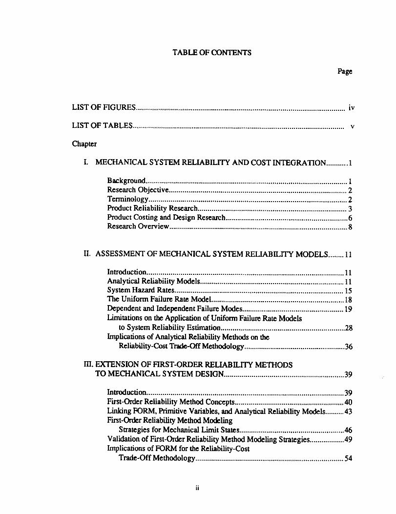
TABLE OF CONTENTS
Page
LIST OF FIGURES ........................................................................................................ iv
LIST OF TABLES ......................................................................................................... v
Chapter
I. MECHANICAL SYSTEM RELIABILITY AND COST INTEGRATION ........... 1
Background .................................................................................................... 1
Research Objective ......................................................................................... 2
Terminology ................................................................................................... 2
Product Reliability Research ........................................................................... 3
Product Costing and Design Research ............................................................. 6
Research Overview ......................................................................................... 8
II. ASSESSMENT OF MECHANICAL SYSTEM RELIABILITY MODELS ........ 11
Introduction .................................................................................................. 11
Analytical Reliability Models ......................................................................... 11
System Hazard Rates .................................................................................... 15
The Uniform Failure Rate Model ................................................................... 18
Dependent and Independent Failure Modes ................................................... 19
Limitations on the Application of Uniform Failure Rate Models
to System Reliability Estimation ............................................................... 28
Implications of Analytical Reliability Methods on the
Reliability-Cost Trade-Off Methodology .................................................. 36
llI. EXTENSION OF FIRST-ORDER RELIABILITY METHODS
TO MECHANICAL SYSTEM DESIGN ............................................................ 39
Introduction .................................................................................................. 39
First-Order Reliability Method Concepts ....................................................... 40
Linking F'ORM, Primitive Variables, and Analytical Reliability Models .......... 43
F'Lrst-Order Reliability Method Modeling
Strategies for Mechanical Limit States ..................................................... 46
Validation of First-Order Reliability Method Modeling Strategies .................. 49
Implications of FORM for the Reliability-Cost
Trade-Off Methodology .......................................................................... 54
IV. PHYSICS-BASEDRELIABILITY MODELING...............................................56
Introduction .................................................................................................. 56
Review of Physics-Basod Failure Rate Reliability Prediction Techniques ........ 57
Linking Physics Failure Rate Methods andTraditional Reliability Techniques ............................................................ 58
Assumptions Made in l)edving Physics Failure Rate Techniques ................... 64
Implications of Physics-Based Methods for the Reliability-Cost
Trade-Off Methodology .......................................................................... 66
V. INTEGRATED PRODUCT DESIGN: A SEQUENTIAL LINEAR
APPROXIMATION METHOD .......................................................................... 69
Introduction .................................................................................................. 69
Defining Product Cost and Reliability Trade-Off Issues ................................. 70
Improving Product Reliability ........................................................................ 72
Product Design Using Sequential Linear Approximation ................................ 73
Sequential Linear Approximation-Overview .................................................. 76
Applying the Sequential Linear Approximation Method ................................. 80
Implications of the Sequential Linear Approximation Methodology ............... 94
VI. CONCLUSIONS AND FUTURE RESEARCH .................................................. 96
Conclusions .................................................................................................. 96
Future Research ........................................................................................... 98
Appendices
A. COMPENDIUM OF MECHANICAL LIMIT STATES ............................... 99
B. MECHANICAL LIMIT STATES USED INFIRST-ORDER RELIABILITY MODELS ................................................ 152
REFERENCES ............................................................................................................ 156
iii
Figure
1.
2.
3.
LIST OF FIGURES
Page
Two Failure Modes with Separate Aging Mechanisms ......................................... 21
Combined and Individual Failure Mode PDF's .................................................... 24
Hazard Rate for Individual and System Failure When Failure Resets All
Failure Modes ..................................................................................................... 25
4. Combined and Individual Failure Mode PDF's-O(0.1) Case ................................ 26
5. Combined and Individual Failure Mode Hazard Rates-O(0.1) Case ..................... 27
6. Hazard Rate-Normal Distribution (COV--0.10) ................................................... 30
7. Hazard Rate-Normal Distribution (COV=0.20) ................................................... 31
8. Hazard Rate-Normal Distribution (COV=0.30) ................................................... 31
9. Influence of Changes in Mean on Hazard Rates ................................................... 33
10. Bi-Modal Time to Failure Distribution ................................................................ 34
1 I. Bi-Modal Distribution Hazard Rate ..................................................................... 35
12. Sequential Linear Approximation Method ........................................................... 80
iv
Table
LIST OF TABLES
Page
1. Limit State Kolmogorov-Smimov Test Results .................................................. 51
2. Monte Carlo and FORM Failure Probability Differences ..................................... 53
3. Pump Shaft Initial Variable Parameters .............................................................. 81
4. Pump Shaft Permissibility Matrix ....................................................................... 84
5. Most Probable Point Vector Values ................................................................... 85
6. Probability of Failure Sensitivities-First Iteration Results .................................... 88
7. Cost Sensitivities-First Iteration Results ............................................................. 89
8. Updated Most Probable Point Vector Values ..................................................... 92
9. Updated Pump Shaft Variable Parameters .......................................................... 93

CHAPTERI
MECHANICAL SYSTEMRELIABILITY AND COSTINTEGRATION
The development of new products is dependent on product designs that
incorporate high levels of reliability along with a design configuration that meets
predetermined levels of system life-cycle costs. Additional constraints on the product
include explicit and implicit performance requirements. In response to the increasing
awareness of product reliability and cost, numerous techniques have been advocated as
methodologies best suited to address the need for improved reliability or cost estimates.
Despite the availability of diverse approaches to product reliability and cost predictions,
little work on integrating product cost and performance has been done.
The separation of reliability and cost prediction methods results in no direct
linkage existing between variables affecting these two dominant product amibutes.
Techniques linking cost and reliability would provide engineers with information on the
trade-off that exists between variables affecting product performance and cost, thereby
permitting a rational design approach for complex mechanical systems.
Research Obiecfive
The objectiveof theresearchistodevelop a methodology to permitmanufacturing
costand reliabilitywade-offsina component design.
We now define the following tem_ology that will be used:
A mechanical system is an organization of multiple subsystems, which in turn
may be composed of multiple components, so as to be capable of performing a specified
physical function.
Reliabifity is the probability that a component will perform in a satisfactory
manner for a given period of time when used under specified operating conditions.
Primitive variables are the stochastically independent variables that define the
behavior of a system. The variables are not only stochastically independent, but also
independent in terms of their physical properties.
A response surface describes the behavior of a system as a function of several
primitive variables.
A failure mode is a physically measurable system behavior that requires the
termination of system use.
A failure mechanism is a predictable, physical deterioration in a system which if
unrepaired results in failure of the system from a specific failure mode.
Analytical reliability models predict failures based on the system time to failure
distribution.
2
Physics-basedfailure rate reliability methodspredictsystemfailureratesbased
onahistorical system failure rate modified by correction factors that consider alternative
primitive variable values.
Product Reliabili_ Research
The development of reliability assessment and prediction methods has been a
recent area of investigation. The reliability techniques currently used can be traced
through two distinctive historical paths. The first developmental path evolved from an
examination of the failure of mechanical systems and developed analytical reliability and
physics-based failure rate techniques. The second developmental path considered the
problems inherent in assessing structural reliability and developed first order reliability
methods. We will briefly review each of these different evolutionary processes.
The initial interest in the study of reliability was undertaken to examine the
question of machine maintenance. Khintchine I and Palm 2 attempted to use methods
suggested I_y Erlang and PaLm that had focused on the problems associated with telephone
u'unking problems.
At the same time Lotka suggested the use of renewal theory as a means of
modeling equipment replacement problems. 3 Other early authors who considered using
renewal theory to model equipment replacement problems were Campbell 4 and Feller. s
The study of extreme value theory was initiated by Weibull 6 7 and Gumbel. s
WeibuU was to propose the extreme value distribution named after him, as best describing
the fatigue behavior of materials.
3
The advent of World War II increased interest in assessing and predicting
mechanical system reliability. The realization that a high percentage of military equipment
was never used, due to its being unserviceable, was a major impetus to examining
reliability methods. 9 The wartime experience led the Air Force to form an ad hoc Group
on Reliability of Electronic Equipment in 1950. In 1951 both the Navy and Army began
investigating equipment reliability issues. In order to coordinate these various
investigations, the Department of Defense, in 1952, established the Advisory Group on
Reliability of Electronic Equipment (AGREE). 1° The first report from AGREE was
published in 1957, and established minimum reliability requirements, testing procedures,
and suggested requiring equipment suppliers demonstrate a confidence level for equipment
reliability. The report suggested using mean time between failures as the equipment
reliability measure.l_
The result of the initial AGREE report was to begin requiring reliability assessment
and engineering in military applications. More importantly, it began a ongoing
investigation of reliability methods by the Depar_nent of Defense (DOD) that has resulted
in periodic reassessment of procedures for prediction and evaluation of reliability.
Following the introduction of the AGREE report, the DOD reissued the report as a
military standani, M[I_STD-781, which has been subsequently revisedJ e
In addition, the introduction of MIL-STD-785B: Reliability Programs for Systems
and Equipment, mandated the integration of reliability planning and assessment in the
engineering design and development of a productJ 3 Its aim was to allow for the earlier
determination and detection of reliability problems.
4

Thedesireby theDOD to developpredictivemethodologiesled to the creation of
physics-based failure rate models that allow for component reliability predictions
depending on operating and design primitive variable values. The initial effort in
developing physics-based failure rate models focused on models for electronic equipment
and these efforts led to the release of MIL-HDBK-217. Recently, a similar approach has
been proposed for use with mechanical components, beginning in 1990 with the release of
the Handbook of Reliability_ Prediction Procedures for Mechanical Eouipment. _4
In the development of structural reliability methods, the initial interest focused on
the development of engineering theory to accurately reflect the conditions existing in
various structural elements. This initial interest in stress analysis understood that loading
and strength were uncertain, but that the situation could be realistically modeled if upper
and lower limits on load and strength respectively were considered. Is Given this approach
to reliability, the engineering community strove to develop a set of design codes that set
out the requirements for different strucuaal designs, with the inclusion of appropriate
safety factors to accommodate the diverse sources of uncertainty in the design.
Two problems hindered the development of probabilistic reliability techniques.
Ftrst, the error in the mathematical models of engineering phenomenon is unknown.
Second, with a system subjected to a wide variety of possible failure modes, using
statistical methods to predict its reliability seemed infeasible. _
In 1967 Cornell proposed the second-moment approach to reliability assessment. _
Lind then proposed a way of relating the safety index suggested by Comell to regular
safety factors suggested in most building codes. _s
_ly following this work, the problem of invariance of the reliability index
was ur_vered by both Ditlevsen 19and Lind. z° The invariance problem was finally
resolved by Hasofer and Lind. 21
The solution of the reliability problem using first-order methods for non-linear limit
states is presented by Rackwitz and Fiessler." The authors present an algorithm to
update estimates of the most probable point using a gradient search approach.
The determination of system reliability estimates for systems with 2 limit states was
presented by Ditlevsen. _ The case involving numerot_s limit states was solved by
deriving upper and lower bounds by Cruse et al._
Thus, by the 1990's the underlying reliability concepts had been established for
mechanical systems using analytical and physics-based failure rate reliability methods, and
for structural systems using probabilistic methods. The extension of probabillsfic methods
to mechanical systems remained to be examined.
Product Costing and Desi_ Research
Methods to determine product configuration and cost have evolved recently into
several divergent areas. The design and costing methods currently in use can be identified
as belonging to three distinctive approaches, namely design-based, tirne-bas_ and cost-
based methods. All three methods have been recent areas of research interest.
In 1983 Boothroyd presented a report entitled "'Design for Assembly" 25 which
presented a method to evaluate competing product designs with respect to ease of
assembly. The methodology focuses on reducing the number of parts used in a

component,with emphasison simple assembly methods. An alternative approach to
assessing assembly ease of design was proposed by Hitachi in 1983. _ The Hitachi
approach, known as 'Assemblability Evaluation Method', has been favored owing to its
lower level of complexity as compared to the Boothroyd approach. Both methods focus
exclusively on product design with respect to assembly, and do not consider product cost
in assessing a proposed design configuration.
Time-based methods focus on reducing the product development time through the
application of techniques such as concurrent engineering. The idea underlying concurrent
engineering is that the majority of the product cost is determined in the concept stage of
product development, and that sequential development processes increase product
development time. 2_Tune-basod methods view time reduction as critical to the success of
a product in the marketplace. 28
Cost-based methods, such as target costing, were developed to examine ways of
incorporating final product cost into the product development process. 29 Such methods
do not consider the impact of product performance on cost, but rather they seek to
allocate product manufacturing costs to each assembly or component.
By the 1990's several competing methodologies exist to manage product
development. The integration of product cost and reliability into a comprehensive and
analytically rigorous framework remained to he examined.
Research Overview
Inorder todevelop a designmethodology thepermitscostand reliabilitytrade-
offs,we must firstexamine existingreliabilityestimationtechniques.In chapter2 we
review analytical reliability models as they are presently being used for mechanical
systems. We examine the statistical concepts that form the foundations of this approach,
and consider the limitations and shortcomings inherent in applying analytical reliability
models. We shall demonstrate that four limitations of analytical reliability models preclude
theft use in assessing the impact of design changes on component reliability. First,
analytical reliability methods do not consider the physical variables that define component
behavior. We shall show that the absence of physical variables in analytical methods
prevents assessment of changes in variables values on reliability. Second, analytical
methods do not consider component operating conditions. Third, analytical methods are
only applicable in the estimation of the reliability of systems that have attained a steady-
state failure rate. We will demonstrate that many mechanical systems operate in a
u'ansient failure rate regime, for which the application of reliability estimates based on
analytical methods is inappropriate. Fourth, analytical methods do not consider the impact
of variance reduction on component reliability. We will examine how the absence of
variance information in analytical methods prevents their use in assessing primitive variable
variancechanges on reliability.
Chapter 3 examines theextensionof first-orderreliabilitymethods (T-ORM) to
rnechanicalsystem design. CmTenfly, themajorityofapplicationsof FORM have bccn in
structuralproblems,with few mechanical phenomena being analyzed.We will

demonstrate methods to model specific r_.,chanical limit states, and determine the validity
of alternative limit state modeling strategies. We will show how the use of FORM
provides one of two major elements of the proposed design paradigm by providing a
means of calculating the reliability sensitivity to changes in the distributional paran_tcrs of
the primiuve variables. We will detailed how FORM techniques are a less resuictive
means of assessing component reliability.
In chapter 4 we will examine the physics-based failure ram reliability estimation
method. We will demonstrate that although physics-based methods provide a means of
assessing the impact of changes in the primitive variable means, they have two major
limitations. First, we will show that physics-based methods are only applicable for
changes in the mean value of a primitive variable. Second, physics-based methods suffer
from a large degree of uncertainty in their estimated based failure rates due to the small
sample sizes used. We will demonstrate that these two limitations preclude the application
of physics-based methods in the reliability-cost trade-off methodology.
Chapter 5 presents the proposed sequential linear approximation method for
assessing component design. We will show how the proposed methodology incorporates
two elements to assess component design, reliability and cost. The first principle elerrcnt
of the methodology is the utilization of FORM results to determine the reliability
sensitivities to changes in primitive variable distributional paran_ters. The second element
is a means of determining the manufacturing cost sensitivities to changes in the primitive
variable distributional parameters. The method will demonstrate that the sensitivity of the
cost to design changes is rcqui_red to determine how the design should be modified. The
9
totalproductcostis not required to assess the component design. We will demonstrate
how these two elements can be combined into an overall methodology to permit
reliability-cost trade-off analysis. A sequential linear approximation methodology is
presented to determine the product configuration with respect to either cost or reliability.
An example problem is presented to demonstrate the application of the methodology.
Chapter 6 concludes by briefly reviewing the research findings and identifies areas
forfurtherresearch.We willreview how theproposed designmethodology utilizes
FORM and costinginformationtoprovideengineerswith an effectivemeans of addressing
thereliability-costtrade-offproblem. We conclude with some suggestionsforfuture
research.
10
CHAPTERII
ASSESSMENTOF MECHANICAL SYSTEM RELIABILITY MODELS
In order to determine the appropriate method for the prediction of mechanical
system reliability, we must first define the existing methodologies in use. We will begin
by outlining common statistical concepts used in reliability estimation which will be
referred to throughout this document. Next, alternative reliability models based on
differing system component arrangements will be examined. The uniform failure rate
model based on the exponential distribution will be examined. The assumptions and
limitations that are inherent in the application of uniform failure rate models to reliability
estimation practice are detailed. Finally, the implications of the limitations of uniform
failure rate models and their application to mechanical systems is discussed.
Analytical Reliability Models
Any component subject to failure has a random time to failure, t, and the time to
failure of the component has a failure probability density function, (PDF),f(O, defined as
f(t)=P(t=t) t>O (2.1)
11
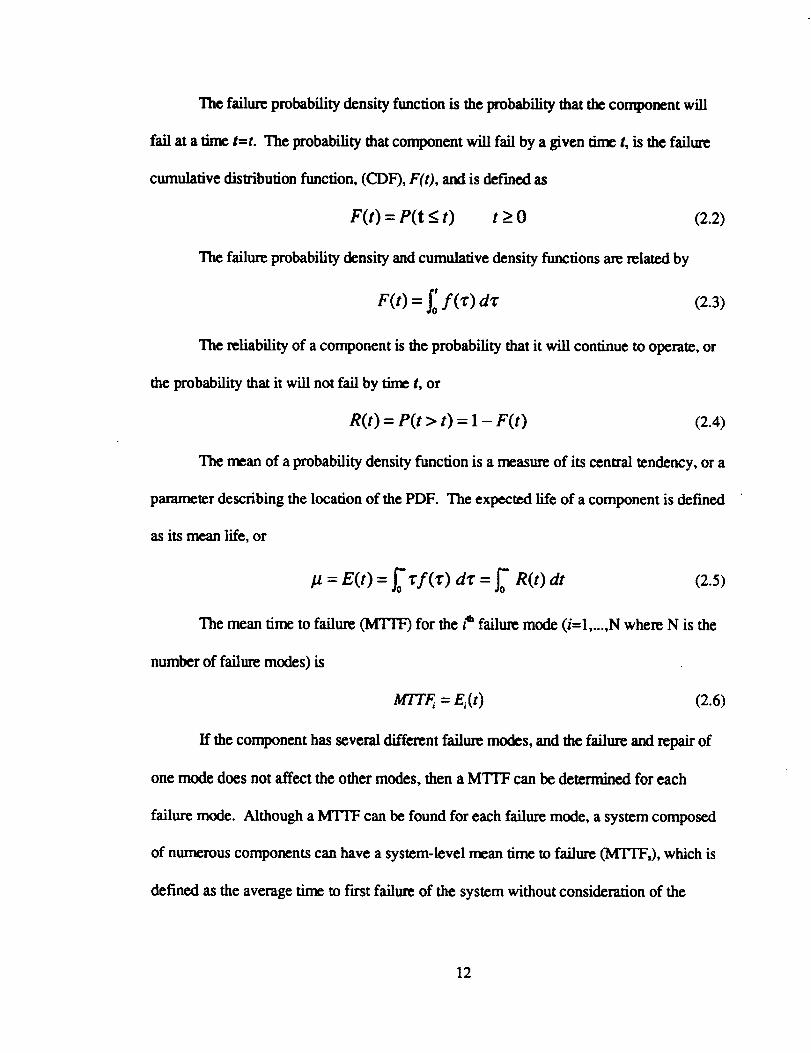
The failure probability density function is the probability that the component will
fail at a lime t=t. The probability that component will fail by a given time t, is the failure
cumulative disuibution function, (CDF), F(t), and is def'med as
F(t)=P(t<t) t>_O
The failure probability density and cumulative density functions arc related by
F(t) = _ f('c) d_
(2.2)
(2.3)
The reliability of a component is the probability that it will continue to operate, or
the probability that it will not fail by time t, or
R(t) = P(t > t) = 1 - F(t) (2.4)
The mean of a probability density function is a measure of its cenu'al tendency, or a
parameter describing the location of the PDF. The expected life of a component is defined
as its mean life, or
= E(t) = _ _f(_) d_: = _ R(t) at# (2.5)
The mean time to failure (hfI3V) for the 4h failure mode (i=1 ..... N where N is the
number of failure modes) is
MTTF_ = Ei(t ) (2.6)
If the component has several different failure modes, and the failure and repair of
one mode does not affect the other modes, then a MTIT can be determined for each
failure mode. Although a MTFF can be found for each failure mode, a system composed
of nun_rous components can have a system-level mean time to failure (M'IWF,), which is
defined as the average time to fast failure of the system without consideration of the
12
failure mode. The mean time between failure (MTBF) is the average of the mean time to
failure for the system due to all failure modes and for any number of failure tLrnes. Letting
I.tTjrepresent the weighted time to the j'_ failure of a system, then if m generations of parts
are repaired or replaced, the MTBF can be determined as 3°,
MTBF = I ___IZTj (2.7)• ,6 ._1
When the system being considered is perfectly renewed through repair and
maintenance, the expected life is equivalent to both the MTFF, and the MTBF.
The failure rate is the probability that a component will fail in a given period of
time. The hazard rate is defined as the instantaneous failure rate, and is given as31
h(t) = f (t_..._) (2.8)
R(t)
The hazard rate is the probability that a component surviving to a specific time, t,
will fail in the next small time interval, t+dt.
Quantifying the degree of dispersion of a variable is done by determining its
variance. The variance of a random variable, t is defined as 32
(2.9)
The square root of the variance is simply defined at the standard deviation, o.
When more than one possible event may affect a component, or system, it is
important to be able to determine the interaction between the various event variables as
well as the individual impact of any specific variable. If the variables are independent, then
changes in one variable value are independent of the other variable, that is changes in one
13
variable will have no effect on any other variable. When two variables are independent
their joint PDF is the product of their individual PDFs, or 33
fx.r(x,y) = fx(x), fi(y) (2.10)
linear relationship between any two variables is described by twoA treasure of the
related parameters, covariance and correlation. IfX and Y are two random variables
having means gx and txr, then the covariance of X and Y is defined as _
Cov(X,Y): E[(X- I._)(Y- I.I,)]: E(XY)- I.ld.I, (2.11)
Since covariance is not dimensionless, a dimensionless measure of the linear
relationship termed the correlation coefficient is often used. The correlation coefficient is
Cov(X,Y)p(X,Y)= (2.12)
definedas3s
Gx . ar
The correlation coefficient has a range of values between -1 and +1, and is a
measure of the linearrelationshipbetween two random variables.Ifp---!-_l,then thetwo
variablesare linearlyrelated;ifO=0, thenthereisno linearrelationship,but thisdoes not
precludethe possibilitythe variablesmay be relatedina non-linearmanner. Iftwo
variablesare independent,thenboth thecovarianceand the correlationare 0.
The independence ofthe variablesdoes not reflectwhether itispossibleto have
more thanone event occurringata particulartime. Ifwe denote theprobabilityof an
event A occurringas P(A), and thatof event B occurringas P(B),then we see thatthe
two possibleoutcomes involvingthesetwo event arethatthey areindependentand have
no intersection,or theyare independentand have some intersection.The occurrence of
14
the intersection event is not related to the independence of the two events, since an
intersection probability can occur even if the events are independent.
System Hazard Rates
We consider the determination of the hazard rates for a system composed of a
number of components. The two alternative system configurations that will be considered
are, series and parallel.
The parallel system configuration requires that only one system component be
functioning in order for the system to operate. If a paraUel arrangement of n components
is assume, d, the system reliability is36
Rs(t) = 1 - Qs(t) = 1 - P[tl < t c_ t2 < t_.. .C'_tn < t]
If the events are assumed to be independent, then the reliability becomes,
Rs(t) = 1- P(tl < t). P(t2 < t)---P(tn < t)
Recall that the reliability of a single component is
Ri(t) = P(ti > t)
(2.13)
(2.14)
(2.15)
Substituting equation (2.15) into equation (2.14) yields the following equation for
the system reliability,
/1
Rs(t) = 1- l"I[1 - Ri(t)] (2.16)
i=1
For the parallel case, the determination of the system hazard rote is not easily
accomplished. This is due to the fact that no similar derivation to that outlined in equation
(2.16) can be found for the parallel configuration case.
15
The series configuration requires that all system components be functioning in
order for the system to operate. If a series arrangement of n components is assumed, and
the time histories of the components are assumed to be independent, then the hazard rate
for the system can be determined. Initially, let the assumption be added that the time each
I
elements of the system has been operating is the same. If t represents the time to failure of
the i_ component, then the reliability for n components is3_
Rs (t)= P(t, > t)c_ P(t2 > t)c_.._P(t. > t) (2.17)
R s (t)= P[h > t _t2 > t_...nt. > t] (2.18)
If the events axe assumed to be independent, then the system reliability becomes
Rs (t)= P(h > t). P(t2 > t).....P(t. > t) (2.19)
Recall that the reliability of a single component is
Ri (t) = P(ti > t) (2.20)
Hence the system reliability is
n
Rs(t) = l'I Ri(t)i=l
Now taking the logarithms of equation (2.21) gives
n
In Rs(t)= _'_In Ri(t)i=l
For any component the reliability can be expressed as
Or alternatively
Ri(t)= ex[_-_ h(l:)dl:]
(2.21)
(2.22)
(2.23)
16
_ h(_:)d_: = - In Ri(t)
h(t) = -d In Ri(t)dt
Substituting equations (2.24) and (2.25) into equation (2.22) yields
n d-d In Rs(t) = _.,---In Ri(t)
dt i=l dt
This yields a system hazard rate
n
hs(t) = _hi(t)'
(2.24)
(2.25)
(2.26)
(2.27)
i=1
Therefore, the system hazard rote is the sum of the component hazard rates if the
following assumptions are made:
1. a series system configuration is used
2. the components are assumed to have independent event histories
3. the components are assumed to have the same initial starting time.
If the assumption that the components have the same starting time is not valid and
the replacement or starting time of component i is t_,, the relationship given in equation
(2.27) becomes,
hs(t) = £ h_(t - tn) (2.28)i=1
The system hazard rate relationships derived in equations (2.27) and (2.28) are
usually difficult to apply since the hazard functions are complex. However, most of the
difficulties encountered in applying the relationships for the system hazard rate can be
17
avoided if the underlying component time to failure distribution is assumed to be
exponential.
The Uniform Failure Rate Model
We will now examine system hazard rates when the underlying time to failure
distribution is assumed to be exponential and then define the uniform failure rate model.
The form of the exponential PDF is given by 38
] -t
f(t) = -_-eT t < 0 ,71,> 0 (2.29)
If the exponential PDF is assumed for the time to failure of the components, then
the results from equations (2.8), (2.23), and (2.29) can be used to determine the individual
hazard function for a component to be,
1
hi (t)= MTTF_ = _-. (2.30)
where the failure rate of the exponential distribution is defined as _.. If we assume a series
system configuration, independent component event histories, common component
starting times, and all components exhibiting exponential time-to-failure PDF's, we can
use the results of equation (2.27) to determine the system hazard rate to be,
n 1 n 1
From equations (2.30) and (2.31), the system M'ITF can be defined as
A
i=l
(2.31)
(2.32)
18
The application of system hazard rate relationships under the assumption of an
cxponential component time to failure distribution is defined as the uniform failure rate
model approach to system reliability estimation.
Dc_lgndent and Independent Failure Modes
The results for the system hazard rate and _ apply to cases where the system
is composed of a number of units, each unit possessing its own t_me-to-failure PDF.
Multiple failure modes can result in a different system reliability depending on the
interaction of the failure modes. Two aitemative failure mode interactions are possible:
I. The failure modes are independent, Under this condition, the failure and repair
of the system with respect to one failure mode renews the time history of the
corresponding failure mechanism. The time histories of the remaining failure
modes acting remain unchanged.
2. The failure modes are dependent. Under this condition, the failure and repair of
the system with respect to one failure mode renews the time history of all active
failure mechanisms. If the time history is reset, the effect is one of perfect renewal
of the system, however the repair of a failure typically does not result in perfect
renewal of the system.
For the case of dependent failure modes, repairing the system due to any failure
results in the entire system being renewed. For example, a sealed ball bearing used to
support a heavy rotating shaft. The two failure modes which affect the bearing would be
19
spalling of the ball bearings and failure of the bearing seal. A failure of the bearing due to
either of these two failure mechanism results in replacement of the entire bearing
assembly. Upon replacement, the time histories of both the spalling and seal failure
r_chanisms are reset.
Dependency of failure modes does not imply either corre lal_i_ between the failure
mechanism, or common random variables. The dependency of the failure modes is not
determix_ by the interaction effects of the random variables, but is a specification of the
type of replacement/repair policy employed and the pliysical limitations of the systems. In
the case cited of the ball bearing, the failure of the bearing seal or due to spalling may be
due to separate and independent failure mechanisms involving stochastically and physically
independent random variables. The failure of the bearing due to either failure mechanism
would physically necessitate the replacement of the entire bearing assembly, thereby
resetting the failure time histories for all active failure modes.
Determining the conditions under which either of the two cases of failure mode
dependency hold is necessary in order to correctly apply reliability prediction methods.
Specifically, we seek to determine the restrictions inherent in the application of reliability
techniques based on uniform failure rate models. Simulation models were developed for
both the dependent and independent failure mode conditions. Two different failure modes
were assumed to affect the hypothetical system under consideration.
Ftrst, we will examine the case of the independent failure modes. Second, we will
examine the case of dependent failure modes. Finally, we will examine the impact of
2O
changes in the failure probability density function distribution parameters on system failure
rate and MTBF.
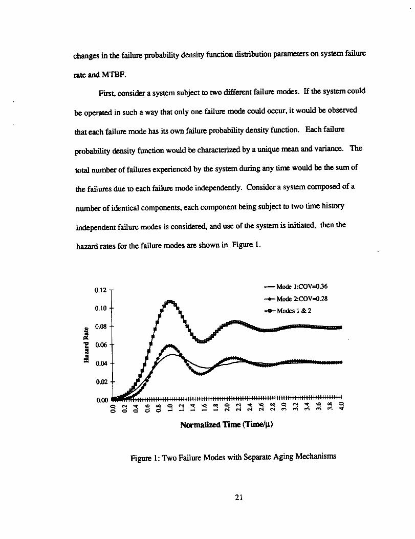
F'trst, consider a system subject to two different failure modes. If the system could
be operated in such a way that only one failure mode could occur, it would be observed
that each failure mode has its own failure probability density function. Each failure
probability density function would be characterized by a unique mean and variance. The
total number of failures experienced by the system during any time would be the sum of
the failures due to each failure mode independently. Consider a system composed of a
number of identical components, each component being subject to two time history
independent failure modes is considered, and use of the system is initiated, then the
hazard rates for the failure modes are shown in Figure 1.
A
ee
0.12
O.lO
0.08
o.06
0.04
0.02
o.0o
O O
_Mode 1:COV=0.36
-4_ Mode 2:COV=0.28
Modes I & 2
Normalized Time (Time/p.)
Figure 1" Two Failure Modes with Separate Aging Mechanisms
21
Theindividualfailuredensityfunctionswereassumedto havethesamemean
value, _t, but different coefficients of variation. Given that each failure density function
has the same mean, the hazard rate of the system due to each individual failure mechanism
should eventually stabilize at its failure rate, or 1/_t. Since the repair of a component due
to a single failure mechanism does not affect the time history of the remaining failure
mechanism, the expected number of units failing due to both failure modes at any time is
the sum of the individual failure rates. Once the system has reachod a steady-state failure
rate, its behavior can be approximated by an exponential failure density function. Under
the assumptions of independent failure modes and approximation of steady-state behavior
by the exponential density function, the system hazard rate is
1 1 2hs(t) = h,(t) + h,(t)=--+-- =-- (2.33)
From equation (2.32) system MTBF is
1 2 (2.34) rrBFs h,(t) U
Note in Figure 1, that there is a transient period following start-up of the system
during which time the individual and system failure rates are not constant. This transient
behavior was noted by Kaput and Lamberson 39 Since the MTBF of a system is a
constant, it can be concluded that the use of MTBF for estimating system reliability
behavior is valid, a long time following start-up, for series systems with independent
failure modes, but is not appropriate for predicting system behavior during the transient
period of operation.
22
Now considerasystemwherethefailuremodesaredependent;the failure and
repair of the system due to either failure mode results in the time histories of both failure
nw,chanisms being reset. Each failure mechanism has its own time-to-failure distribution
described by a unique mean and variance. However, when considered as system subjected
to two failure mechanisms simultaneously, the system behavior is characterized by the time
to first failure resulting fi'om the failure of either of the two possible failure mechanisms.
The resulting failure rate for the system cannot be determined by the application of the
results for series systems which were derived earlier, equations (2.27) through (2.32),
since the relative contribution to the overall system failure rate is dependent on the mean
and standard deviation of each failure mode. This case represents a situation of
conditional reliability, since the probability of failure due to a failure mode is dependent on
the system having not previously failed.
Consider two cases, the first where the area of intersection of the two failure mode
probability density functions is 0(1), the second where the area of intersection of the two
failure mode probability density functions is 0(0.1). Note that O denotes the order measure
of the area of intersection of the two time-to-failure PDF's. Thus 0(0.1) would signify
that the area of intersect was in the range of 0-1% of the total PDF area. Complete
intersection of the PDF's would be denoted as O(10).
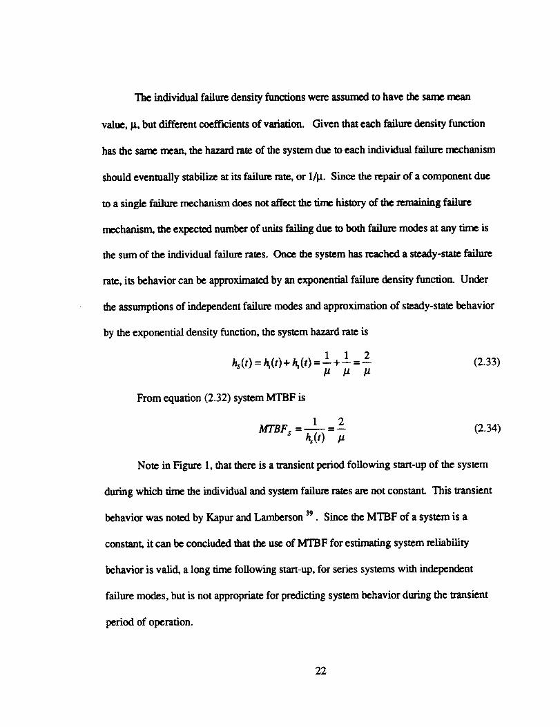
When the area of intersection of the two failure mode PDF's is 0(1) both failure
n'r..chanisms conu'ibute to the system behavior. Consider the following 0(1) PDF area of
23
intersectioncase. Monte Carlo simulation was used to determine the two failure
mechanisms PDF's as wen as the resulting system PDF's shown in Figure 2.
0.05 T _ -a-Mode 1:U_=1.25, Cov--0.32
0.05 t // _\ --Mode 2:p,=l.O, COV--O.20
II \\0.04 _Modes 1 & 2
o.o_t tl _,\"_o.o_t II
t ly0.020.01
0.01
0.{30
0.00 0.25 0.50 0.75 1.00 1.25 1.50 1.75 2.00 2.25 2.50
Normalized Time (Time/g2)
Figure 2: Combined and Individual Failure Mode PDF's
Note that the system failure PDF is different from both failure PDF's due to the
fact that the system can exhibit failures from each of the two failure mechanisms. The
resulting hazard rate for a system comprised of nurmrous identical components, each of
which subjected to the two dependent failure modes is depicted in Figure 3.
24
0.06
0.05
0.04
0.03
[] 0.02
0.01
0
Normalized Time (Timedl, t2)
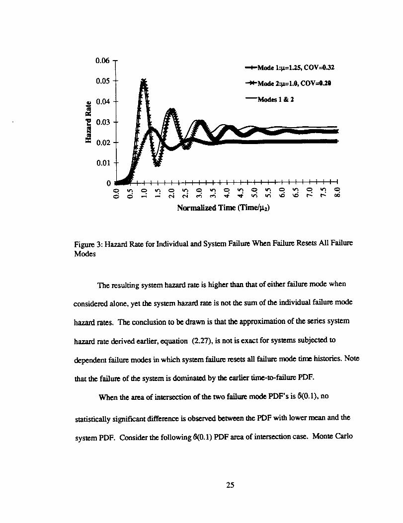
Figure 3: Hazard Rate for Individual and System Failure When Failure Resets All Failure
Modes
The resulting system hazard rate is higher than that of either failure mode when
considered alone, yet the system hazard rate is not the sum of the individual failure mode
hazard rates. The conclusion to be drawn is that the approximation of the series system
hazard rate dedvod earlier, equation (2.27), is not is exact for systems subjected to
dependent failure modes in which system failure resets all failure mode time histories. Note
that the failure of the system is dominated by the earlier time-to-failure PDF.
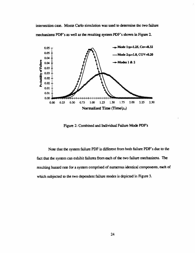
When the area of intersection of the two failure mode PDF's is 8(0.1), no
statistically significant difference is observed between the PDF with lower mean and the
system PDF. Consider the following 8(0.1) PDF area of intersection case. Monte Carlo
25
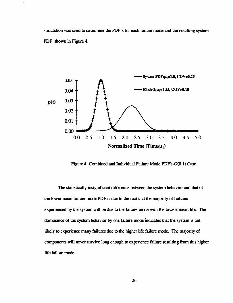
simulation was used to determine the PDF's for each failure mode and the resulting system
PDF shown in Figure 4.
p(t)
--4--" System PDF:I/,t=I.0, COV--0.7.00.05
0.04 _ : = -
0.03
0.02
0.01
0.00
0.0 0.5 1.0 1.5 2.0 2.5 3.0 3.5 4.0 4.5 5.0
Normalized Time (Time311_)
Figure 4: Combined and Individual Failure Mode PDF's-O(0.1) Case
The statistically insignificant difference between the system behavior and that of
the lower mean failure mode PDF is due to the fact that the majority of failures
experienced by the system will be due to the failure mode with the lowest mean life. The
dominance of the system behavior by one failure mode indicates that the system is not
likely to experience many failures due to the higher life failure mode. The majority of
components will never survive long enough to experience failure resulting from this higher
life failure mode.
26
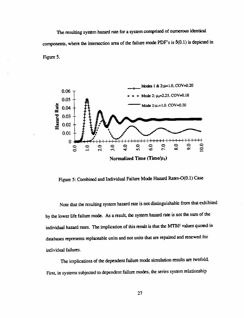
The resulting system hazard rate for a system comprised of numerous identical
components, where the intersection area of the failure mode PDF's is _(0.1) is depicted in
Figure 5.
Modes 1 & 2:p=l.O, COV=0.20
0.06 ""+'-
00 tA -- Mode l:u,=l.O. COV--0.20
0.04
0.02
..0
Normalized Time (Time/pl)
Figure 5: Combined and Individual Failure Mode Hazard Rates-O(0.1) Case
Note that the resulting system hazard rate is not distinguishable from that exhibited
by the lower life failure mode. As a result, the system hazard rate is not the sum of the
individual hazard rates. The implication of this result is that the MTBF values quolod in
databases represents replaceable units and not units that are repaired and renewed for
individual failures.
The implications of the dependent failure mode simulation results are twofold.
First, in systems subjected to dependent failure modes, the series system relationship
27
clef'ruing the system hazard rate (equation (2.27)) is not applicable. Second, in cases of
multiple failure modes, the overall system hazard rate closely approximates the behavior of
the failure mode with the lowest MTTF.
From these simulation results, the following conclusions can be drawn:
1. Use of MTBF for estimates of system reliability based on the summation of
component MTBF values is only valid for series systems in which the failure
modes are independent.
2. Use of MTBF for predicting the system behavior during the transient period of
system start-up and operation is not appropriate.
3. Use of the lowest MTBF values are appropriate for estimating system
reliability.
Limitations on the Application of Uniform Failure Rate Models to System Reliability_Estimation.
In &e simulation results presented, once the sysmm was activated, a transient
period during which the system did not display s_dy-state hazard rate behavior occurred.
Eventually the system auained a steady-state hazard rate, at which point the behavior of
the system could be reasonably approximated by the uniform failure rate modeL Since we
concluded that the transient period of system behavior could not be estimated using
MTBF, we would like to determine the transient response behavior of the system. If the
transient period were found to be of extremely short duration when compared with the
component MTFF, then it may be argued that the overall system behavior can be
28
reasonableapproximatedbyusingtheuniformfailureratemodel. If thedurationof the
u'ansientperiodis notsubstantiallyshorterthanthecomponentMTTF, thenwewouldlike
todetermine if it is possible to estimate system reliability using MTBF estimation methods.
We will now examine the impact of changes in the failure probability density
function diswibufion parameters on the system failure rate and system MTBF. We wiU
examine how the system wansient response behavior is affected by the underlying failure
probability density function, and whether or not the system witl ever approach steady-state
conditions. The assumptions underlying this analysis are:
i. The system behaviorcan be describedby a singlePDF.
2. There areseveralidenticalcomponents inoperation.
3. All components are activated at the same time.
4. Failed units are replaced or perfectly renewed instantaneously.
5. The time the system operates is much greater than the component MT1T.
We willexamine theimpact of thetime tofailurePDF coefficientof variationand
mean on both the time requiredtoreach a steady-statehazardrate,and themaximum
hazard rateexperiencedby thesystem. We willdefinethe time toreach steady-stateas
the time required by the system to exhibit a ± 5% deviation in peak-to-peak hazard rate.
First, consider the impact of changes in the coefficient of variation of the
component time to failure distribution on the time to attain steady-state hazard rate
conditions. A normal failure distribution wiU be assumed. Initially, the impact of
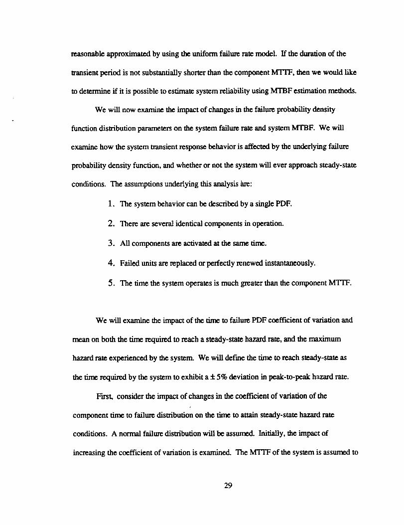
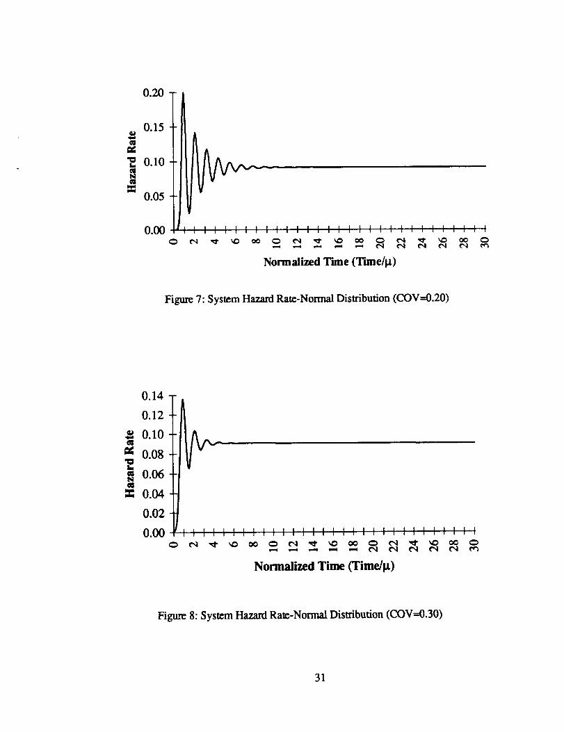
increasing the coefficient of variation is examined. The MTFF of the system is assumed to
29
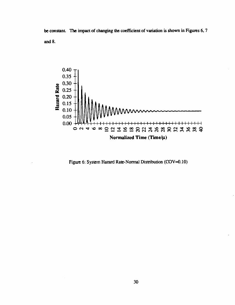
be constant. The impact of changing the coefficient of variation is shown in Figures 6, 7
and 8.
0.40
0.35
0.30
0.25
0.20
_0.15
0.10
0.05
0.00_eq
Normalized Time (Time/l_)
Figure 6: System Hazard Rate-Normal Distribution (COV=0.10)
30
at
L.
t_
m
Normalized Tune (T'une/_)
Figure 7: System Hazard Rate-Normal Distribution (COV=0.20)
0.14
0.12
0.10
0.08
0.06
_ 0.04
0.02
0.00
Normalized Time (Time/It)
Figure 8: System Hazard Rate-Normal Distribution (COV=0.30)
31
Note that decreasing the coefficient of variation by a factor of 2 from 0.2 to 0.1,
results in higher maximum failure rate (40% .vs. 20% of the population). Decreasing the
coefficient of variation by a factor of 2 resulted in an increase in the time to reach steady
state by a factor of 3.
If all units are started at the same time, it is possible that by sufficiently reducing
the coefficient of variation of the component time to failure distribution the system will
never reach a steady-state behavior and will exhibit a regular spike pauem of failures. In
most real mechanical systems, units are started at different times, reducing the impact of
such transient spike failure rates.
As the coefficient of variation is decreased, a threshold value is reached below
which further reductions in the coefficient of variation results in the system never attaining
a steady-state failure rate. For components exhibiting small deviations in life from their
MTFF values, predicting system performance using the uniform failure rate model is not
appropriate.
Second, consider the impact of changes in the component MTIT on the time to
attain steady-state hazard rate conditions. A Gaussian time to failure distribution is
assumed. The impact of increasing the MTFF is examined. The coefficient of variation of
the time to failure distribution is held constant. Compare the system response for the two
different MTYF's shown in Figure 9.
32
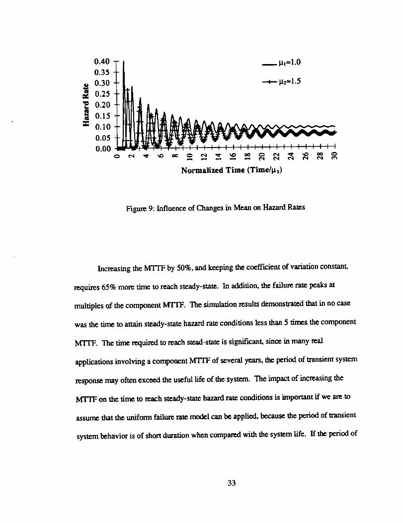
0.40 __ l.tl=l.O
0.35
0.30 =-
0.250.20
0.15
[] 0.10
0.05
0.00
Normalized Time (Time/ttt)
Figure 9: Influence of Changes in Mean on Hazard Rates
Increasing the MTIT by 50%, and keeping the coefficient of variation constant,
requires 65% more time to reach steady-state. In addition, the failure rate peaks at
multiples of the component MTTF. The simulation results demonstrated that in no case
was the time to attain steady-state hazard rate conditions less than 5 times the component
MTI'F. The time required to reach stead-state is significant, since in many real
applications involving a component MTIT of several years, the period of transient system
response may oftenexceed theusefullifeof thesystem. The impact of increasingthe
MTTF on the time toreach steady-statehazard rateconditionsisimportantifwe areto
assume that the uniform failure rate model can be applied, because the period of transient
system behavior is of short duration when compared with the system life. If the period of
33
transient system response accounts for much of the useful life of the system, then clearly
the application of uniform failure rate reliability prediction techniques cannot be justified.
From these simulation results we can conclude that the mean of the failure
distribution is positively correlated with the time required to reach steady-state, while
coefficient of variation is negatively correlated with the time required to reach steady-
state.
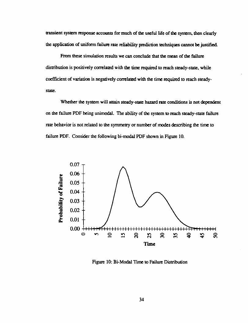
Whether the system will attain steady-state hazard rate conditions is not dependent
on the failure PDF being unirnodai. The ability of the system to reach steady-state failure
rate behavior is not related to the symmetry or number of modes describing the time to
failure PDF. Consider the following bi-modal PDF shown in Figure 10.
0.07
0._
0.05
o._
0.03
0.020.01
0._ _i iiiiiiii
Time
Figure 10: Bi-Modal Time to Failure Distribution
34
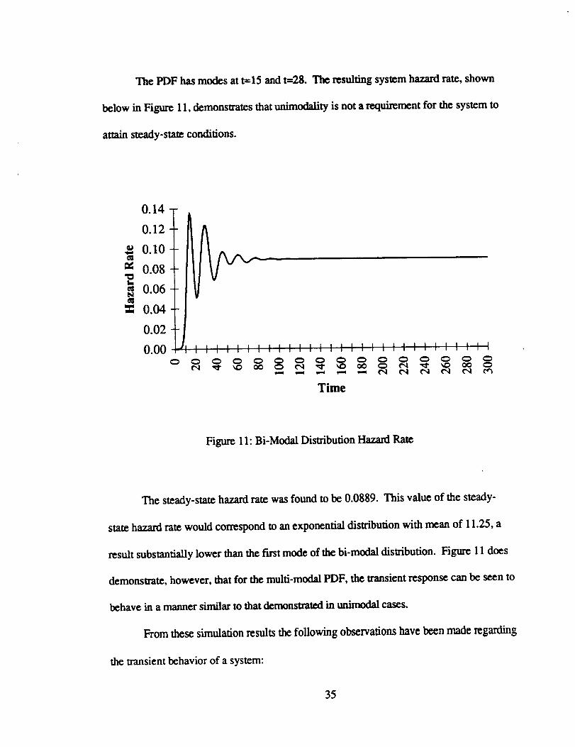
The PDF has modes at t=15 and t=28. The resulting system hazard rate, shown
below in Figure 11, demonstrates that unimodality is not a requirement for the system to
attain steady-state conditions.
0.14 !0.12
0.I0
0.08t..eu 0.06
_ 0.04
0.02
0.00 ,,''lll'''lllll''llllll'''lllIIII II1 II III
Time
Figure 11: Bi-Modal Distribution Hazard Rate
The steady-state hazard rate was found to be 0.0889. This value of the steady-
state hazard ram would correspond to an exponential distribution with mean of 11.25, a
result substantially lower than the first mode of the bi-modal diswibufion. Figure 11 does
demonstrate, however, that for the multi-modal PDF, the wansient response can be seen to
behave in a manner similar to that demonstrated in unimodal cases.
From these simulation results the following observations have been made regarding
the transient behavior of a system:
35
1. Increasing the component MT'FF leads to the system requiring a greater period
of time to attain steady=state conditions.
2. Decreasing the coefficient of variation of the component time to failure results
in a higher maximum failure rate. In addition, the system requires a greater
period of time to attain steady=state conditions if the coefficient of variation is
decreased.
3. In order for a system to attain steady-state conditions, there exists a lower limit
on the coefficient of variation of the component time-to failure distribution.
4. Unimodal and multi-modal PDF's result in the system reaching steady-state.
5. Peaks in the transient failure rates coincide with multiples of the component
MTIt:.
6. The time required to reach steady state conditions is significantly greater than
the MTTF for the system. The time required to reach :t:.5%of the steady-state
failure rate was never less than 5 times the MTTF.
Implications of Analytical Reliabili _tyMethods on the Rel_ia_bility-CostTra_-Off
Having demonstrated the limitations inherent in the application of analytical
reliability methods several implications are evident. We have shown that analytical
reliability methods do not consider the physical variables that define either the failure
modes or operating environment that the component experiences. If we consider
equations (2.6) and (2.32) which define MTrF and the system failure rate, it is clear that
36
the uniform failure rate model does not include physical variables. The inability of the
uniform failure rate model to include physical variables prevents its use to esdmate
component reliabilityresultingfrom changes ineitherprimitivevariablesor operating
environment. This is due to the inability to determine the reliability sensitivity to changes
in the physical variables. Without a means of estimating the impact of changes in variables
on reliability, analytical methods cannot be integrated into a methodology to explore
reliability-cost tradc-offs that result from variable changes.
The absence of physical random variables in the analytical reliability method
precludes thcir use in determining the impact of variance reduction on reliability and cost.
Reduction of variance or truncation of physical variable distributions can affect the
component reliability. Methods ,such as Taguchi methods and statistical process control,
focus on variance reduction or control as a means of reducing cost and improving
reliability. Without distributional information of physical variables in analytical methods,
the cost of variance cannot be determined.
We have demonstrated that analytical reliability methods can only be used to
estimatethe behavior of systems thathave attaineda steady-statefailurerate.Also we
determined that the time to attain steady-state failure rates is significantly greater than the
component MTTF. The fact that the time to achieve steady-state conditions is so long
indicates that most mechanical systems operate in the transient failure rate regime.
Assessing component reliability in the transient failure rate regime cannot be accomplished
with analytical reliability methods, requiring the application of alternative reliability
estimation methods in these cases.
37
Where analytical reliability methods can be used in reliability-cost trade-offs is
when examining alternative existing components versus costs directly rela_i to MTTF.
Analytical methods could then be used to examine different available component
reliabilities as compared to an estimated replacement or warranty cost. In this case, the
reliability-cost trade-off does not consider the configuration or design of the component,
but rather the selection of one of many alternative designs.
Having demonstrated the assumptions and limitations of analytical reliability
methods and their unsuitability for use in a reliability-cost trade-off methodology, we now
examine physics-based reliability methods.
38
CHAPTER HI
EXTENSION OF FIRST-ORDER RELIABILITY METHODS TO MECHANICAL
SYSTEM DESIGN
We have examined analyticalreliabilitymo_Is, and have demonstrated their
inherentlimitationsand underlyingassumptions. These analyticalmethods arenot
physics-basedapproaches toreliabilityestimation.The absence ofphysicalvariablesin
analyticalreliabilitymodels createsseveralweaknesses. First,analyticalreliabilitymodels
areunable tomodel specificoperatingconditionsaffectinga system. Second, analytical
reliabilitymodels areunableto specifythemode of failurefora system. Third,analytical
reliabilitymodels areunabletodeterminetherelativeimportance thatindividualphysical
variablesplayin specificfailuremodes.
To counterthe shortcomingsinvolvedinusinganalyticalreliabilitymodels, we
considerthe applicationofphysics-basedreliabilitymethods tomechanical systems. First,
we willoutlinethe basicconceptsof physics-basedreliabilitymethods. Second, we will
determinethelinkagesthatexistbetween physics-basedreliabilitymethods, primitive
variables,and theuniform failureratemodel. Third, we willbrieflyoutlinethephysics-
based failure models that affect mechanical systems, and define limit states for the failure
models. Fourth, we will examine the validity of alternative modeling strategies for
physics-based limit state models. We seek to demonswate the applicability of physics-
39
based reliability methods to mechanical systems as well as their relationship to analytical
reliability models.
First-Order Reliability Method Concepts
We will consider the fmxlauental principles which define physics-based reliability
models, in particular fwst-order reliability methods (FORM). The reliability of system
components is defined by the limit states that affect the system. A limit state is a
characteristic of the system component which can be observed, and is defmed to represent
the failure of the component due to a specific failure mechanism. The failure of the
component need not be represented by the cataslxophic failure of the component, but may
be defined as a measurable degree of degradation in one or more properties of the
component.
The response function relates a limit state of the system component to the
primitive variables that characterizes tile system perfornmnce. The primitive variables are
defined as being both statistically as well as physically independent variables. The
response function is defined as:
g( )=gtxl,x2.....where X = XI, X 2..... X n = vector of primitive variables
spon funcuon
The limit state of the system is defined as:
whereg(_)>O= SafeState
o=
(3.1)
(3.2)
4O
The limit state relationship given by equation (3.2), is an n-dimensional surface.
One side of the surface is the failure region, on the other side is the safe region. The
joint probability density function of the variables is
pf = probability of failure
=
(3.3)
Note that the probability of the failure state is the volume integral over the failure
_giOn.
The reliability index, [3, represents the minimum distance from the origin to the
limit state function. In order for the reliability index to be invariant, it is necessary for the
primitive variables to be transformed to uncorrelated standard normal variables. If the
variables are correlated they must first be transformed into equivalent uncorrelated
variables. If the variables are nonnormal, then they must first be transformed into
equivalent normal variables using either a two or three parameter fit. Once transformed
into standard normal variables, the limit state function becomes,
g(17) = f(Yl,Y2, .... Yn) (3.4)
The reliability index, 13,is the minimum distance to the lincarized limit state
surface. The point on the linearized limit surface that is closest to the origin is called the
most probable point, y', and satisfies the following relationship,
/5 = min(y *r- (3.5)
41
Determiningthe relationship between the most probable point and the reliability
index involves the gradient vector of the limit state function in standard normal space,
defined as,
' O,_Y2 '''"
Then the reliability index and the most probable point are given as: 4o
y =
Ifwe consideronly a first-orderTaylor seriesapproximation tothe limitstate
functionatthe most probable point,thenthe directioncosinesof theoutward normal
vector at the most probable point are:
aye
(3.6)
(3.7)
(3.8)
The direction cosines, _, represent the sensitivity of the reliability index, 13, to
changes in yi, at the most probable point. This sensitivity measure assumes that the
distribution parameters of the variable concerned remains the same. The direction cosine,
o_, relates the i '_ component of the most probable point, yi, to the reliability index, as
shown in equation (3.9).
42
S
Y i = -ai* ,6 i = 1,2, .... n (3.9)
In addition to being the minimum distance from the limit state to the origin, the
most probable point is used as the expansion point for the Taylor series expansion used to
linearize the limit state function.
The most probable point is found by minimizing the reliability index subject to the
constraint that the point lie on the limit state function, or g(Y)=0. If a linearized
approximation m the limit state function is used, then the direction cosines are constant
along the function making the determination of the most probable point easy. Amongst
the most useful methods used for the linearized limit state case, it that proposed by
Rackwitz and Ficssler 41. If a non-linear approximation to the limit state function is used, if
the limit state constraint is satisfied, then it is possible to use either Lagrangian multipliers
or gradient projection methods to determine the most probable poinL
Li_king FORM. Primitive Variables and Analytical Reliability Models
We now examine the relationship between first-order reliability methods, the limit
state primitive variables, and analytical reliability models. Specifically, we will examine the
relationship between changes in first-order reliability results, changes in limit state
primitive variables, and MTI'F me,asurcs of reliability.
We begin by considering the sensitivity of reliability index to changes in the
parameters of the primitive variables. Although R would be possible to determine the
sensitivity of the reliability index to changes in the primitive variables using numerical
methods, we desire a closed-form solution. A closed-form result for the reliability index
43
sensitivitywouldavoidrepeatedapplicationof FORM necessaryfor estimationof
reliability sensitivities.Let theparametersof theprimitivevariablesbedenotedbyp.
Previously in equation (3.5) the reliability index was defined as
:) (3.10)
The sensitivity of the reliability index to changes in the distribution parameters of a
primitive variable was demonstrated by Madsen et al.42 to be,
d..O_fl0p,(Po) =°r(y*Tcgp`[__. .y')'/2] - _[f(y"_2 +(y2)2o3pk̀_\ 1, " +'''+(y:)2 )1/2] (3.11)
This can be rewritten as:
--*T t) --*
_ifl(po)= N_.___[Y 1 --*T 03 --* 1 *T a T[z*.po)
•(3.12)
Note that y" is the most probable point on the limit state function. In addition T is
defined as the Rosenblatt transformation, which is used to wansform correlated non-
normal variables into equivalent uncorrelated normal variables. Finally, we define z as,
Z* : T'l(._*,po) (3.13)
Madsen et al. also demonstrated the sensitivity of the probability of failure with
respect to the sensitivity factors for the reliability index, given as,
.__oOO0_ip (F(y, po) ) = _i,(_fl(po)). "_q_(-flCPo)) Opi (Po)
where P(F(_, Po)) = probability of failure
q_ = normal cumulative disu'ibution function
¢ = normal probability density function
(3.14)
44
We will now use the results enumerated in equations (3.10) through (3.14) to
determine the sensitivity of the MTI'F to changes in the primitive variables distribution
parameters.
The MTIV of any component is defined as 43,
&_/'irF - _O_: f(_')d_'-- SO R(t)dt - Jo[I- F(t)] dt (3.15)
We seek to determine the sensitivity of MTI'F to changes in the distribution
parameters of one of the primitive variables, p_. The partial derivative of the MTFF with
respect to the primitive variable Pi is given by,
_MTFF(Po) = 3 [00[1 - F(_)]d_ (3.16)i oPi "u
Now recall that the probability of failure of failure for the system evaluated at any
point y and dependent on the primitive variable parameter po is,
Probability of Failure = P(F(_,po)) (3.17)
Substituting equation (3.17) into equation (3.16) yields,
We now apply Liebnitz's rule to equation (3.18) to give,
(3.19)
But the partial derivative of 1 with respect to the primitive variable parameter pi is
zero, so we are left with,
45
Now substituting the results of equation (3.14) into equation (3.20) gives,
_i MTTF(Po) = IO _i -,(po)_ (3.21)
_ii MTTF (P o) - IO ,(-_ (p o) ) _ii,(Po)d'¢ (3.22)
By way of equation (3.22) we have demonstrated the sensitivity of the MTrF to
changes in the primitive variables paran_ters. The linkage of MTTF to both changes in
the primitive variables and the reliability index provides as means of comparing FORM and
analytical reliability methods. In addition, by way of equation (3.22), we have means of
estimating the MTI'F sensitivity to changes in the primitive variable distributional
parameters. This MTTF sensitivity estimate could be used in the reliability-cost trade-off
methodology to incorporate MTTF related costs such as warranty and replacement costs.
First-Order Reliabili_ Method Modeling Strateoes for Mechanical Limit States
Having examined the theoretical basis for fast-order reliability methods as well as
the linkage between FORM and analytical reliability methods, we examine appropriate
methods of modeling mechanical limit states to be employed when conducting FORM
reliability estimates. Specifically, we seek to identify the relationships that can be used to
model the failure modes the define mechanical limit states.
To determine the best modeling approach for first-order reliability methods applied
to mechanical limit states several of the limit states, identified in the compendium of limit
states (see Appendix),were selected and tested. The majority of the limit states that were
deemed relevant to mechanical systems were found to be power law relationships. Two
46
limit states were found to follow Arrhenius relationships, namely, uniform corrosion and
thermal degradation. The limit states that were modeled included:
1. wear
2. fretting wear
3. pitting
4. erosion-corrosion
5. galvanic corrosion
6. low-cycle fatigue
With the exception of low-cycle fatigue, all the noted limit-states were considered
to have a response function of the form:
g( R,S) = R - S (3.23)
In this case R represents either the resistance of the system to the specific
degradation effect being modeled, or some maximum allowable degree of system
deterioration. Similarly, S represents the actual degree of material stress induced on the
system, or the actual degree of degradation of the system due to the degradation process
under consideration.
When R represented the maximum allowable degree of system deterioration, it was
assumed to be a random variable with a specified distribution and parameters. In all limit
states modeled, the actual deterioration experienced by the system, S, was a function of
several random variables. The functional form taken by S was dependent on the particular
mechanical limit state being considered. The exact nature the mechanical limit states
considered is outlined in Appendices A and B.
47
In the case of low-cycle fatigue, the response function was of the form:
g( N MIN ,N ACTUAL) = --N MIN + N ACTUAL (3.24)
Here Nu_v is the _n_um number of cycles the system must operate while in
service, and NAc_ is the number of cycles to failure. N_v was assumed to be randomly
distributed variable, and NACTUALWas a function of several primitive variables.
After extensive examination of the available scientific literature, little information
on the disWibution of specific limit state primitive variables was found. In the majority of
cases where information on primitive variables distribution parameters could not be
found, the variables were assumed to be either normal or log-normally distributed. The
primitive variables defined in each limitstate were assumed to be independent.
The first-order reliability method applied to each response function included both
the mean value first-order method (MVFO) and the advanced mean value first-order
method (AMVFO). If the response function (or Z function) is assumed to be smooth,
then we can take a Taylor's series expansion of the response function at the mean value _.
The mean and variance of the response function can be determined if we consider only the
first-older terms. 4s If the distributions of the primitive variables and their parameters are
det-med, and if we consider only first-order terms in the Taylor series approximation, then
the cumulative density function (CDF) of the response function is also defined. The
estimation of the response function CDF by linear function is referred to mean value first-
order (MVFO) approach.
If the response function is non-linear, then its approximation by a first-order Taylor
series witl result in some error. The inclusion of higher order terms in the Taylor series
48
will improve the accuracy of the analysis, although the approach is more difficult. The
advanced mean value first-order (AMVFO) method includes a simple function, H(ZI), to
approximate the higher order terms of the Taylor series.
The application of first-order reliability methods to each response functions was
conducted using the NESSUS/FPI software developed by Southwest Research Institute
under funding by the NASA Lewis Research Center _. The NESSUS/FPI software allows
for the response function to be incorporated in several alternative formats. The two
approaches that were used are:
1. The user defined subroutine of the form:
g(X)- f(X1,X2,...Xn,Zo)
In this case the response function can have any specified form.
2. A response function of the form:
(3.25)
X1 = f (X2,X3,...Xn,Zo) (3.26)
In the second approach defined in equation (3.26) one primitive variable must be
separable from the others, and the response function written with the separable variable on
the left-hand side. In some cases this is not feasible given the functional form of the limit
state relationship. The various modeling techniques used and the validation of the
techniques used for each limit state are now discussed.
Validation of First-Order Reliability_ Method Modeling Stramoes
The accuracy of the first-order reliability method modeling strategies were
validated using Monte Carlo simulation. In all cases conventional Monte Carlo analysis
49
was used, and no effort was undertaken to use importance sampling approaches. For
each limit state a Monte Carlo simulations using 50,000 samples was employed.
Since many primitive variables distribution parameters were unknown, FORM was
applied assuming normally disu'ibuted variables and again assuming log-normally
distributed variables. Additional FORM analyses were conducted assuming different
coefficients of variation (COV) for the primitive variables. The different coefficients of
variation were used to examine the effect of primitive variable variance on limit state
modeling validity.
A comparison was made between those results obtained using Monte Carlo
simulation and fast-order reliability methods. The cumulative density functions for each
response function modeled were obtained and plotted for both the first-order reliability
method and Monte Carlo simulation.
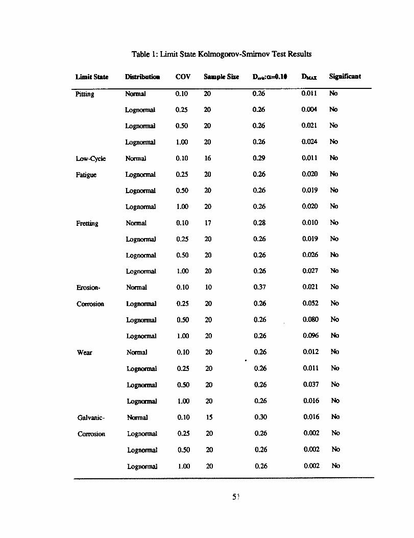
A Kolmogorov-Smirnov test was applied to each limit-state modeled to de:ermine
if the CDF found using fast-order reliability methods differed from that obtained using
Monte Carlo. The Koimogorov-Smimov test considers the maximum difference between
the two cumulative density functions to determine if they are the same, 4_ or:
(3.27)
Here F(x) represents the theoretical or assumed value of the CDF, and S(x) the
observed or experimentally determined value of the CDF.
For the seven limit states considered, the results of the Kolmogorov-Smirnov tests
are given below.
5O
Limit State
Table 1" Limit State Kolmogorov-Smimov Test Results
Distrilmtioa COV Sample Size De_:ct--0.10 D_c_x Sigaificant
Pitting
Low-Cycte
Fatigue
Fretting
Erosion-
Corrosion
Wear
Galvanic-
Corrosion
Normal 0.10 20 0.26 0.011
Lognotmal 0.25 20 0.26 0.004
Lognonnal 0.50 20 0.26 0.021
Lognomml 1.00 20 0.26 0.024
Normal 0.10 16 0.29 0.011
Lognormal 0.25 20 0.26 0.020
Lognonnal 0.50 20 0.26 0.019
Lognormal 1.00 20 0.26 0.020
Normal 0.I0 17 0.28 0.010
Lognormal 0.25 20 0.26 0.019
Lognonnal 0.50 20 0.26 0.026
Log_ 1.00 20 0.26 0.027
Normal 0.10 10 0.37 0.021
Lognormal 0.25 20 0.26 0.052
Lognotmal 0.50 20 0.26 0.080
Lognormal 1.00 20 0.26 0.096
Normal 0.10 20 0.26 0.012
Lognormal 0.25 20 0.26 0.011
Lognotmal 0.50 20 0.26 0.037
Logmmnal 1.00 20 0.26 0.016
Normal 0.10 15 0.30 0.016
Lognormal 0.25 20 0.26 0.002
Lognonnal 0.50 20 0.26 0.002
Lognormal 1.00 20 0.26 0.002
No
No
No
No
No
No
No
No
No
No
No
No
No
No
No
No
No
No
No
No
No
No
No
No
5,_
From these results, we conclude that there is no statistically signifr.ant difference
between the cumulative density functions obtained using first-order and Monte Carlo
methods for each limit state. However, this statistical comparison of first-order and
Monte Carlo methods using the Kolmogorov-Smimov test is based on the maximum
difference in the CDF of the failure distribution, which would occur about the center of
the distribution. We would like to determine the validity of FORM methods when the
probability of failure is very low. This involves examination of the behavior of FORM
methods in lthe tail of the probability of failure distribution, and its comparison with
Monte Carlo results.
Since no statistical test exists to compare two CDF's at low probability values, we
will show the probability of failure results obtained for both FORM and Monte Carlo. In
each case a specific probability of failure was selected from the Monte Carlo results, the
corresponding performance function value (referred to as a Z-level) was noted, and the
corresponding FORM-based probability of failure at the specific performance function
value was found. The two probabilities of failure for the various limit states, and the
precentage difference between them is shown below.
52
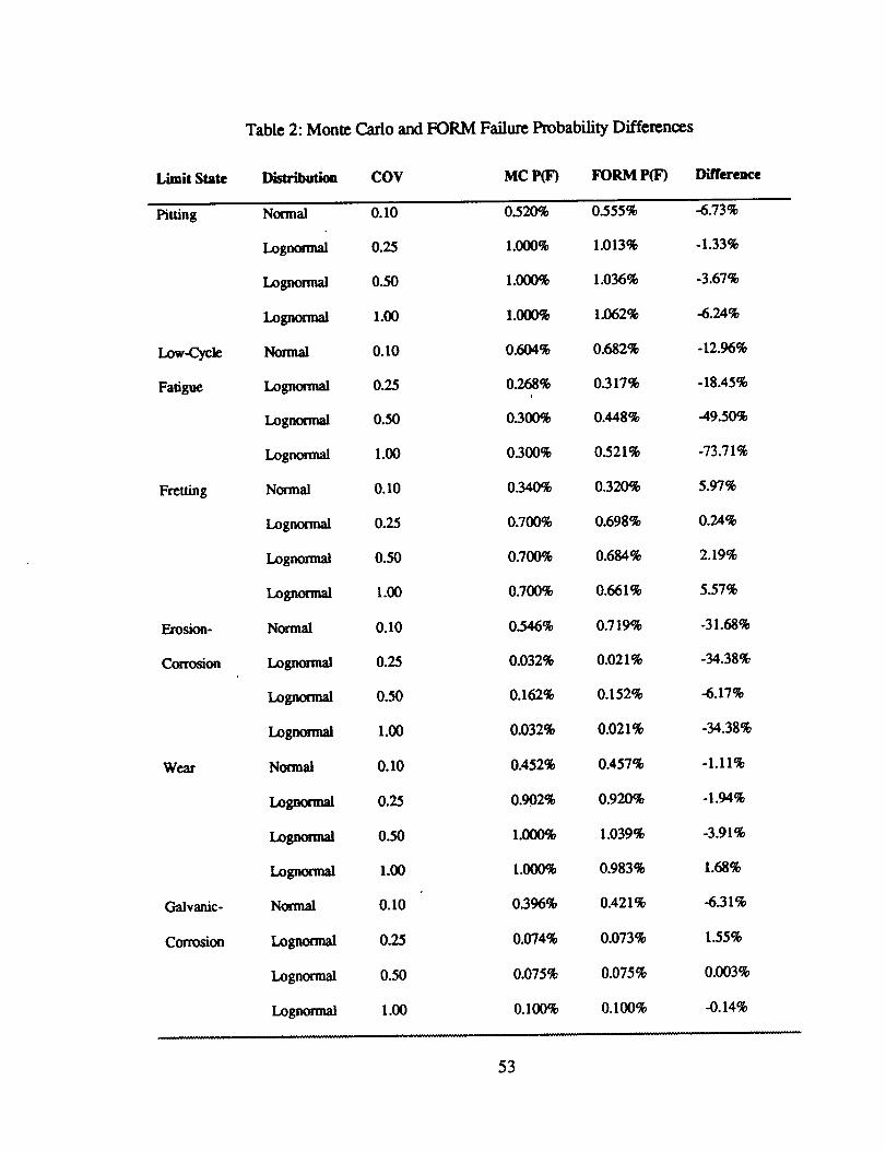
Limit State
Table 2: Monte Carlo and FORM Failure Probability Differences
Distribution COV MC P(F) FORM P(F) Difference
Pitting
Low-Cycle
Fatigue
Fretting
Erosion -
Corrosion
Wear
Galvanic°
Corrosion
Normal 0.10 0.520% 0.555% -6.73%
Lognormal 0.25 1.000% 1.013% -1.33%
Lognormal 0.50 1.000% 1.036% -3.67%
Lognormal 1.00 1.000% 1.062% -6.24%
Normal 0.10 0.604% 0.682% -12.96%
Logm3nnal 0.25 0.268% 0.317% - 18.45%
Lognonnal 0.50 0.300% 0.448% -49.50%
Lognormal 1.00 0300% 0.521% -73.71%
Normal 0.10 0.340% 0.320% 5.97%
Lognormal 0.25 0.700% 0.698% 0.24%
Lognonnal 0.50 0.700% 0.684% 2.19%
Lognonnal 1.00 0.700% 0.661% 5.57%
Normal 0.10 0.546% 0.719% -31.68%
Lognormal 0.25 0.032% 0.021% -34.38%
Lognormal 0.50 0.162% 0.152% -6.17%
Lognonnal 1.00 0.032% 0.021% -34.38%
Normal 0.10 0A52% 0A57% -1.11%
Lognonnal 0.25 0.902% 0.920% -1.94%
Lognot'mal 0.50 1.000% 1.039% -3.91%
Lognorma] 1.00 1.000% 0.983% 1.68%
Normal 0.10 0396% 0.421% -6.31%
Lognormal 0.25 0.074% 0.073% 1.55%
Lognormal 0.50 0.075% 0.075% 0.003%
Lognonnal 1.00 0.100% 0.100% -0.14%
53
From these results, it can be seen that with the exception of low=cycle fatigue and
erosion=corrosion the failure probabilities obtained from FORM and Monte Carlo are
similar. Low=cycle fatigue and erosion-corrosion did display marked differences in their
resulting probabilities of failure. It should be noted that in every case the difference
between FORM and Monte Carlo results was less than an order of magnitude despite the
fact that the results wer compared at low probability of failure values.
Implications of FORM for the Reliability-Cost Trade-Off Methodology
Having demonstrated a relationship for the sensitivity of the _ to changes in
the distributional parameters of primitive variables, as well as identifying and validating
modeling strategies for various mechanical limit states, several implications are evident.
We have the extended first-order reliability method to mechanical systems by
demonstrating and validating specific modeling strategies for a number of mechanical limit
states. The validation of FORM for mechanical systems provides reliability engineers with
a viable alternative to analytical reliability methods.
The sensitivity of component reliability to changes in the distributional parameters
that can be estimated from FORM results provides one of two principle elements required
for the proposed design paradigm. FORM, by providing a means to determine the
reliability sensitivity, provides a means of estimating the impact on component reliability of
changes in the distributional parameters of the primitive variables.
Being a physics-based estimation method, FORM is a less restrictive means of
assessing component reliability. The less restrictive nature of FORM permits its
54
application to both existing and neoteric designs, as well as for systems subjected to
unique operating conditions. FORM can also be used to estimate the reliability of
components at any time in their economic life. This allows FORM to be used to estimate
reliability during the wansient failure rate regime of operation. Reliability estimations for
components in the transient failure regime would provide more accurate measures of
anticipated unit failures, and permit better estimation of maintenance requirements. The
ability to estimate component behavior in the transient failure rate period is in marked
contrast to other reliability methods.
In equation (3.22) we derived a relationship to estimate the sensitivity of the
to changes in the distributional pararaeters of the primitive variables using FORM
results. This relationship can be used in the reliability-cost trade-off method to
incorporate MTI'F related costs, such as warranty and liability costs. The inclusion of such
costs in a trade-off methodology would permit engineers to approximate the impact of
design modifications on non-manufacturing costs. This ability to estimate non-
manufacturing costs provides unique information to engineering and management
regarding the relationship between product design and cost.
Having extended and validated FORM to mechanical systems, and having
demonstrated its principle contributions to the reliability-cost trade-off methodology, we
will now examine physics-based failure rate estimations methods.
55

CHAFFER IV
PHYSICS-BASED RELIABILITY MODELING
Introduction
We have examined analytical reliability methods which focus on mean time to
failure and mean time between failure. Analytical method reliability predictions based on
M'ITF/MTBF do not consider the impact of changes in operating conditions or design
specifications. Consequently, it is difficult for the engineer to use results from analytical
methods to improve a product's design. Using first-order reliability methods does provide
the engineer with information needed to de_ design improvements.
The drawbacks of using FORM techniques are the computational time and effort
required to conduct an assessment of component reliability. A simple computational
approach to measure the impact of primitive variables on component reliability would
provide the engineer with a simple guide to product improvement. Physics-based failure
rate reliability prediction techniques are a likely candidate for such approximate
assessments of component reliability.
To assess the validity of physics-based failure rate reliability prediction techniques
we will examine the assumptions required for their successful application to mechanical
systems. First, we will outline the basic concepts of physics-based failure rate reliability
prediction techniques. Second, we will establish linkages between physics-based failure
rate reliability prediction techniques and analytical reliability models by way of example.
56
Third,wewill outlinetheassumptionsthat must hold in order to apply physics-basod
reliability prediction techniques to mechanical systems.
Review of Physics-Based Failure Rate Reliability_ Prediction Techniques
Previously we examined analytical reliability models. We demonstrated that the
analytical reliability models were linked to the component time to failure PDF, and were
directly influenced by its distribution parameters. Analytical reliability models do not
incorporate primitive variables accounting for differing component designs or operating
environments. A methodology that incorporates design and environment primitive
variables is physics-based failure rate reliability prediction techniques, hereafter referred to
as physics failure rate techniques.
Analytical reliability techniques depend on measures of component and system
MTrF to assess reliability. Physics failure rate techniques use failure rates as a n'easure of
component reliability. Unlike analytical reliability techniques, physics failure rate
techniques derive a component failure rate by modifying a base failure rate by a number of
correction factors. Each correction factor represents the anticipated deviation of a specific
design or environmental primitive variable fi'om the conditions under which the base
failure rate was determined. The physics failure rate is that outlined in the H_ndbook of
Reliability_ Pre0iction Procedures for Mechanical Eo_uipment 48.
The failure rate models axe typically of the form:
i.,i
where: ;kc_,_=failure rate of componem
57

_.o_-base failure ram of component
C_=correction factor i.
In order to predict the component failure rate, kco_, it is necessary for the
engineer to know:
1. The component base failure rate, _
2. The values of the design and environnm_t primitive variables for the
component base failure rate
3. The values of the design and environment primitive variables under which
the component will operate.
The consideration of changes in component primitive variables allows the engineer
to measure the impact of changes in variable values on component reliability.
To use physics failure rate techniques it is apparent that some form of empirical
data on component failure rates is required. In addition to empirical data on component
failure rates, information regarding the service or experimental conditions under which the
data was gathered is also needed.
Linking Physics Failure Rate Methods and Traditional Reliability_ Techniques
We now determine the relationship between physics failure rate methods and
analytical reliability methods. Specifically, we seek to determine the assumptions and
limitations that must hold in order for physics failure rate methods to be valid. We will
first determine the general form that the physics failure rate models must follow in order to
58
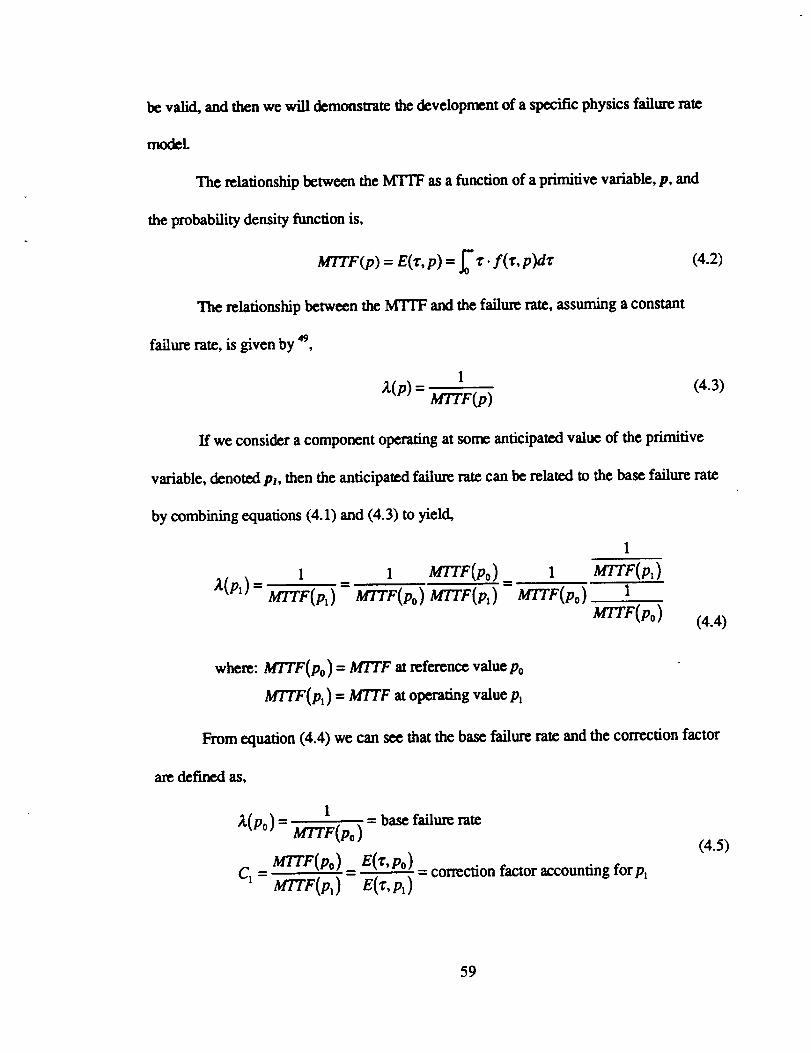
be valid, and then we will demonstrate the development of a specific physics failure rate
model
The relationship between the MTTF as a function of a primitive variable, p, and
the probability density function is,
MTrF(p)= E(_,p) = _ z. f(_, p)d_ (4.2)
The relationship between the MTrF and the failure rate, assuming a constant
failurerate,isgiven by 49,
I,_(p)=
M_r(p)(4.3)
If we consider a component operating at some anticipated value of the primitive
variable, denoted Pl, then the anticipated failure rate can be related to the base failure rate
by combining equations (4.1) and (4.3) to yield,
1 1 MTTF(Po)a,Cp_)= MTTF(p_)=MrTF(P0)MrrF(p_)=
1 MTTF(pl)
_:rrr(po) 1MTTF(Po)
(4.4)
where: MTTF(p o) = MTTF at reference value P0
MTTF(p_) = MTTF at operating value Pl
From equation (4.4) we can see that the base failure rate and the correction factor
are defined as,
1
:t(P°) = MTTF(po ) = base failure rate
M'ITF(Po) E(_',Po) =correction factor accounting for Plc, = MrrF(p,)= e(_,p,)
(4.5)
59
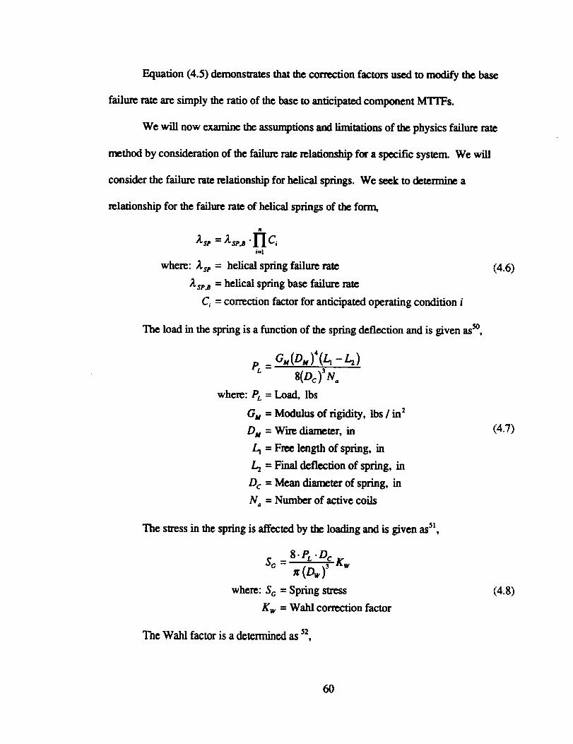
Equation (4.5) demonstrates that the correction factors used to modify the base
failure rate are simply the ratio of the base to anticipated component M'FFFs.
We will now examine the assumptions and limitations of the physics failure rate
method by consideration of the failure rate relationship for a specific system. We will
consider the failure rate relationship for helical springs. We seek to determine a
relationship for the failure rate of helical springs of the form,
Zsr --Zsr , .l Ici=1
where: Xsp = helical spring failure rate
2sp _ = helical spring base failure rate
Ci = correction factor for anticipated operating condition i
The load in the spring is a function of the spring deflection and is given asso,
8(Dc )3 N.
where: PL = Load, Ibs
Gu = Modulus of rigidity, lbs / in _
D M = Wire diameter,in
/.,I= Free lengthof spring,in
L2 = Finaldeflectionof spring,in
D c = Mean diameter of spring,in
N a = Number of activecoils
The stressin the springisaffectedby the loadingand isgiven ass_,
where: So = Spring stress
Kw = Wahl correction factor
The Wahl factor is a determined as 52,
(4.6)
(4.7)
(4.8)
60
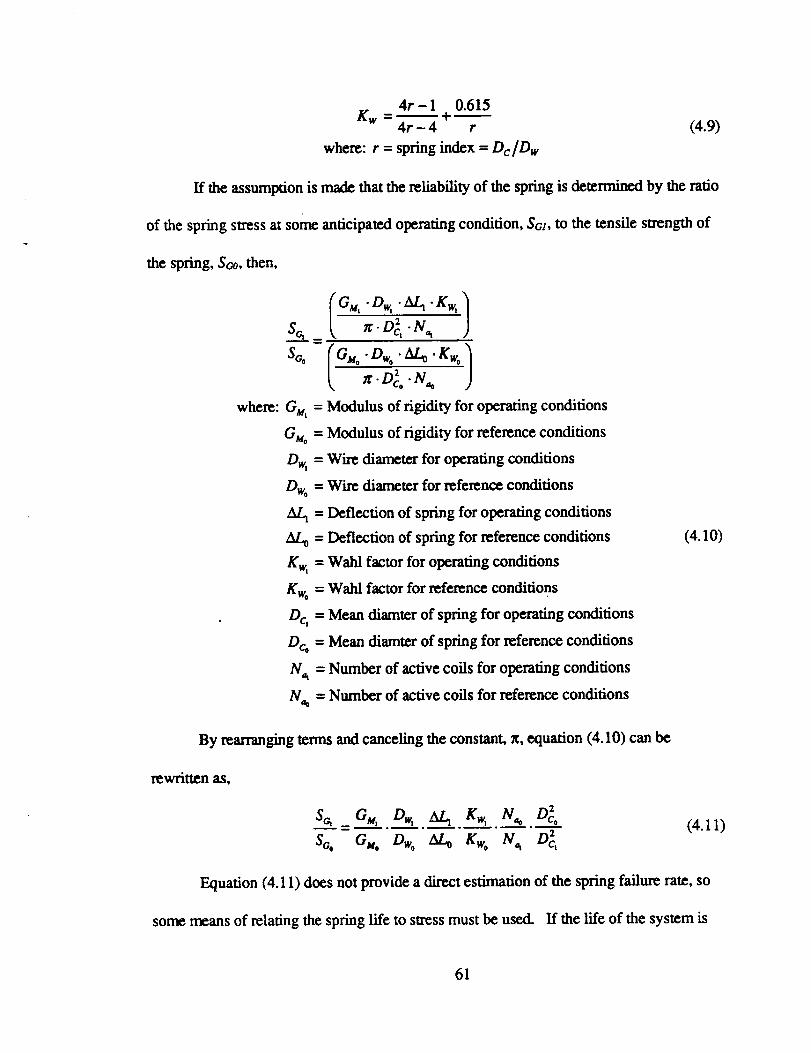
4r- I 0.615fw =--+.--
4r-4 r
where: r = springindex --Dc/Dw
(4.9)
If the assumption is made that the reliability of the spring is determined by the ratio
of the spring stress at some anticipated operating condition, Sc_, to the tensile strength of
the spring, Soo, then,
where:
m_
GMI _"
G_ =
Dw-
Dw° -
-
Kw_ =
Dc, =
N_
IGMo .Dwo" M._. Kwo;g. D 2 • No,Co
Modulus of rigidity for operating conditions
Modulus of rigidity for reference conditions
Wire diameter for operating conditions
Wire diameter for reference conditions
Deflection of spring for operating conditions
Deflection of spring for reference conditions
Wahl factor for operating conditions
Wahl factor for reference conditions
Mean diamter of spring for operating conditions
= Mean cliamter of spring for reference conditions
= Number of active coils for operating conditions
= Number of active coils for reference conditions
(4.10)
By rearranging terms and canceling the constant, x, equation (4.10) can be
rewritten a.%
S_ Gu, Dw, Al.q Kw, N, o DeCo
$60 Gsl° Dwo ALo Kwo N_ D 2c,
(4.11)
Equation (4.11) does not provide a direct estimation of the spring failure rate, so
some means of relating the spring life to stress must be used. If the life of the system is
61
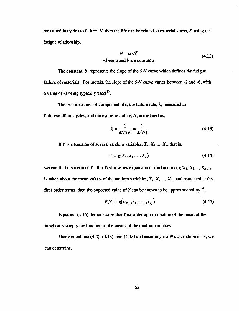
measuredincyclesto failure,N, then the life can be related to material stress, S, using the
fatigue relationship,
N =a.S b(4.12)
where a and b are constants
The constant, b, represents the slope of the S-N curve which defines the fatigue
failure of materials. For metals, the slope of the S-N curve varies between -2 and -6, with
a value of-3 being typically used 53
The two measures of component life, the failure rate, X, measured in
failures/million cycles, and the cycles to failure, N, are related as,
1 12 = _ = _ (4.13)
MTTF E(N)
If Y is a function of several random variables, XI, X2 ..... X,, that is,
Y = g(Xl,X 2..... X,) (4.14)
If a Taylor series expansion of the function, g(X:, X2 ..... X, ),we can find the mean of Y.
is taken about the mean values of the random variables, X_, X2 ..... X,, and truncated at the
first-order terms, then the expected value of Y can be shown to be approximated by 54,
E(Y) =_g(t_x, ,btx2 ..... btx. ) (4.15)
Equation (4.15) demonstrates that first-order approximation of the mean of the
function is simply the function of the means of the random variables.
Using equations (4.4), (4.13), and (4.15) and assuming a S-N curve slope of-3, we
can determine,
62
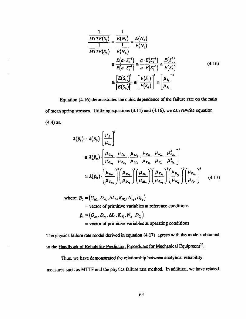
1 1
m'rr(s_)=__E(N,)_ e(No)1 1 E(N,)
m'rp(So) e(No)_e(a.#)_ a.e(#)_ e(S_)- e(a.s?)- ,, e(s?)- E(s;)
t ,s.,r--[e(So)]'-Lg(So)J=
(4.16)
Equation (4.16) demonslrates the cubic dependence of the failure rate on the ratio
of mean spring stresses. Utilizing equations (4.11) and (4.16), we can rewrite equation
(4.4) as,
3Z(p,)= 2,,(_o)L_-_J
--X(po)L_o.. "..'ST"/a_,o /_ ,ujr,,° ,uN., /Ja_,J
(4.17)
where:t0= (G,..D,.._.K...N,.Oc.)= vector of primitive variables at reference conditions
P, =(GIe,,Dw,,ALI,Kw,,N,,,Dc,)
= vector of primitive variables at operating conditions
The physics failure rate model derived in equation (4.17) agrees with the models obtained
in the H_ndbook of Reliability. Prediction Procedures for Mechanical Eo_uipmcnt 55.
Thus, we have demonstrated the relationship between analytical reliability
measures such as M'ITF and the physics failure rate method. In addition, we have related
63
the correction factors employed by the physics failure rate method to the changes in the
primitive variables and the mean of the component probability density function.
Assumptions Made in Deriving Physiq_ F_lure R_te Techniques
We have outlined the basic concepts of the physics failure rate technique as well as
linking it to analytical reliability models. We now examine the assumptions and conditions
that must hold in order for the physics failure rate techniques to yield valid results.
First, the base failure rate and the primitive variable values at the reference
condition must be known. A consequence of this is that generic database failure rates
cannot be used to establish the base failure rates of components since they do not include
information on the primitive variable values at the reference condition.
Second, in order to estimate the expected life of a component, the physics failure
rate models use a first-order Taylor series approximation of the performance function
defining component life. For highly non-linear performance functions, the expected value
of the component life based on a Taylor series approximation should include higher order
terms.
Third, the models use a life relationship which defines the component life as a
function of several primitive variables. The utilization of a life relationship allows for the
incorporation of primitive variables into the failure rate model.
Fourth, as demonstrated in equation (4.17), each correction factor represents the
ratio of a primitive variable mean value at the reference condition to its mean value at the
operating conditions. Hence, the physics failure rate models do not incorporate any
64
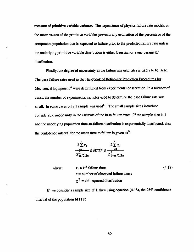
measure of prirnifive variable variance. The dependence of physics failure rate models on
the mean values of the primitive variables prevents any estimation of the percentage of the
component population that is expected to failure prior to the predicted failure rate unless
the underlying primitive variable distribution is either Gaussian or a one paran_ter
distribution.
Finally, the degree of uncertainty in the failure rate estimates is likely to be large.
The base failure rates used in the Handbook of Reliability_ Prediction Procedures for
Mechanical Equipment _ were determined from experimental observation. In a number of
cases, the number of experimental samples used to determine the base failure rate was
small. In some cases only 1 sample was used 5_. The small sample sizes introduce
considerable uncertainty in the estimate of the base failure rates. If the sample size is 1
and the underlying population time-to-failure distribution is exponentially distributed, then
the confidence interval for the mean time to failure is given asSS:
n n
2_,Xi 2_,Xi
i=1 _<MTTF _< i=12 2
_, a12,2n X l-a/2,2n
where: x i = i th failure time (4.18)
n = number of observed failme times
Z 2 = chi- squared distribution
If we consider a sample size of 1, then using equation (4.18), the 95% confidence
interval of the population MTrF:
65
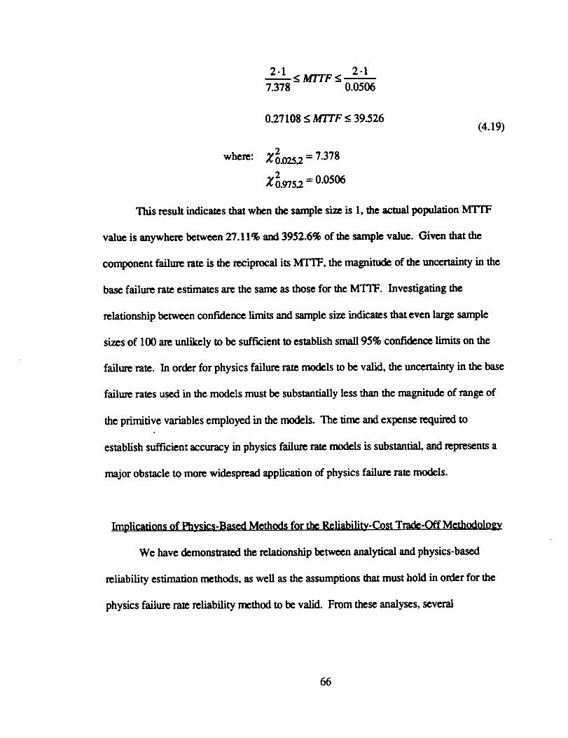
2-1 2-I--< MTTF_<--7.378 0.0506
0.27108 < MTTF < 39.526
where: Z 2 = 7.378O.O25,2
_2 = 0.05060.975,2
(4.19)
This result indicates that when the sample size is 1, the actual population M'VrF
value is anywhere between 27.11% and 3952.6% of the sample value. Given that the
component failure rate is the reciprocal its MTrF, the magnitude of the uncertainty in the
base failure rate estimates are the same as those for the MTFF. Investigating the
relationship between confidence limits and sample size indicates that even large sample
sizes of 100 are unlikely to he sufficient to establish small 95% confidence limits on the
failure rate. In order for physics failure rate models to he valid, the uncertainty in the base
failure rates used in the models must he substantially less than the magnitude of range of
the primitive variables employed in the models. The time and expense required to
establishsufficientaccuracy inphysicsfailmeratemodels issubstantial,and representsa
major obstacleto more widespread applicationof physicsfailureratemodels.
Implications of Physics-Basod Methods for the Reliabiliw-Cost Trade-Off Methodology
We have demonstrated the relationshipbetween analyticaland physics-based
reliability estimation methods, as well as the assumptions that must hold in order for the
physicsfailureratereliabilitymethod tobe valid.From theseanalyses,several
66
implications for the applicability of physics failure rate methods to product design are
evident.
Although the physics-based failure rate methods incorporates primitive variables in
its reliability estimates, equation (4.17) demonstrates that the method is only applicable for
changes in the mean value of the primitive variables. As such, physics-based failure rate
methods do not consider the impact of changes in variance or truncation of the variables
on component reliability. The inability to deumnine the effect of variance reduction or
truncation on component reliability is a limitation on the use of physics-based methods in
any u'ade-off methodology.
The changes in primitive variables are with respect to an established base
component configuration, which are obtained from available historical databases of
component failure rates. The reliance on historical databases for the base failure rate
values imposes two limitations on physics-based methods. First, neoteric component
designs cannot be analyzed since no historical failure data exists. Second, reliability
estimates cannot be made for systems with anticipated operating conditions that differ
from those reflected in the base failure values. These limitations preclude the
incorporation of physics-based methods in the wade-off methodology.
As we have demonstrated, the physics-based failure rate method suffers from a
large degree of uncertainty in the estimated base failure rates. The large degree of
uncertainty in the estimated base failure rates is the result of the small sample sizes used.
In order to ensure that the magnitude of the uncertainty in the estimated base failure rates
are substantiallylessthan theallowablerange of primitivevariables,thenumber of
67
samples required will be several orders of magnitude larger than those comprising existing
failure rate databases. The urgertamty in the physics-based failure rate ngthod is larger
than the range of feasible change in the primitive variables. Hence any estimation of the
impact of changes in the primitive variables cannot be statistically distinguished from the
random error in the methodology. Such large estimating errors precludes the inclusion of
the physics-based failure rate method in a trade-off methodology.
We have examined the validity of analytical, physics failure rate, and first-order
reliability methods. Having demonstrated the assumptions and restrictions of each
method, we will now examine how engineers and managers can incorporate reliability
estimation methods into the product design.
68
CHAPTER V
INTEGRATED PRODUCT DESIGN: A SEQUENTIAL LINEAR APPROXIMATION
METHOD
We have examined both analytical and physics-based reliability techniques from the
perspective of usefulness to the designer/engineer. These methods allow the engineer to
improve the performance of a proposed product, yet the impact of design changes
motivated by performance criteria that include product cost has not been addressed.
Considered in isolation, methodologies based solely on engineering evaluations of
performance are unlikely to yield a product that represents an acceptable compromise
between cost and performance.
We begin by defining the cost/reliability problem encountered in product design.
Second, we outline the various means of improving product reliability. Third, a
methodological approach to rationally explore product reliability/cost trade-offs and
determine the product configuration is presented. Fourth, an example problem
demonstrating the application of the design methodology is presented. Finally, we outline
the implications of the use of the suggested methodology on design, manufacturing, and
product management.
69

Defining Product Cost and Reliability_ Trade-Off Issues
We examine the nature of the reliability and cost trade-off problem that confronts
engineers and management. In Chapter 1, a number of alternative methods have been
suggested to incorporate cost considerations in the product design process. Most methods
focus on product simplification or target costing as the fundamental means of controlling
product cost. 59_o Yet these approaches do not consider the interaction between product
performance and cost, and offer no systematic approach to assessing the impact of
product configuration changes on cost.
There are three current approaches to product configuration management. First,
design based methods, such as design for manufacture, focus on restricting product design
to a subset of feasible product configurations. The underlying premise of design based
techniques is that the restriction of acceptable product configurations to a subset
composed of simplified component designs results in lower manufactmSng costs. Several
shortcomings of this approach have been pointed out, most importantly, that focusing on
reducing product assembly may yield designs requiring longer development lead times,
thereby lowering net present values for the future income stream from the product. 6t
Second, time-based methods, such as concurrent engineering, focus on
coordinating and paralleling design activities in order to minimize the lime needed to
introduce a product The assumption of time-based methods is that product market share
is determined by the rapidity with which new products are introduced, and the time a
product may have an effective monopoly due to the absence of competitors.
Concentrating on development time can result in poor product design due to inadequate
70

testing. Evidence on time-based product development indicates market advantages accrue
to the firms introducing neoteric products, ca By contrast, many products are evolved
from previous designs, conditions wherein improved product performance would confer
marketing advantages. The inability of time-based development techniques to assess and
improve the design configuration of a product is an obstacle to its implementation as an
engineering-management tool.
Third, cost=based methods, such as target costing, focus on restricting overall
product cost and allocating component cost as a portion of the total product cost. Target
costing requires management to identify the appropriate selling price and the resulting
manufacturing cost of the product prior to the initiation of the design process. 43 64 The
overall manufacturing cost is then allocated among the component parts. The problem in
applying cost-based approaches to product design is the preference it places on reducing
manufacturing costs without considering product performance.
The difficulty confronting engineers is that no existing techniques provide
guidelines to enhancing product performance and assessing the impact of design changes
on product cost. In order to undertake the rational design of a product, engineers and
management require a design methodology that provides a consistent, technically valid
means of assessing a product design configuration, and to rationally explore trade-offs
between product reliability and cost. In assessing component reliability the designer
would like to address two fundamental questions. First, determine the minimum cost
required to attain a desired level of product reliability. Second, the maximum reliability
71
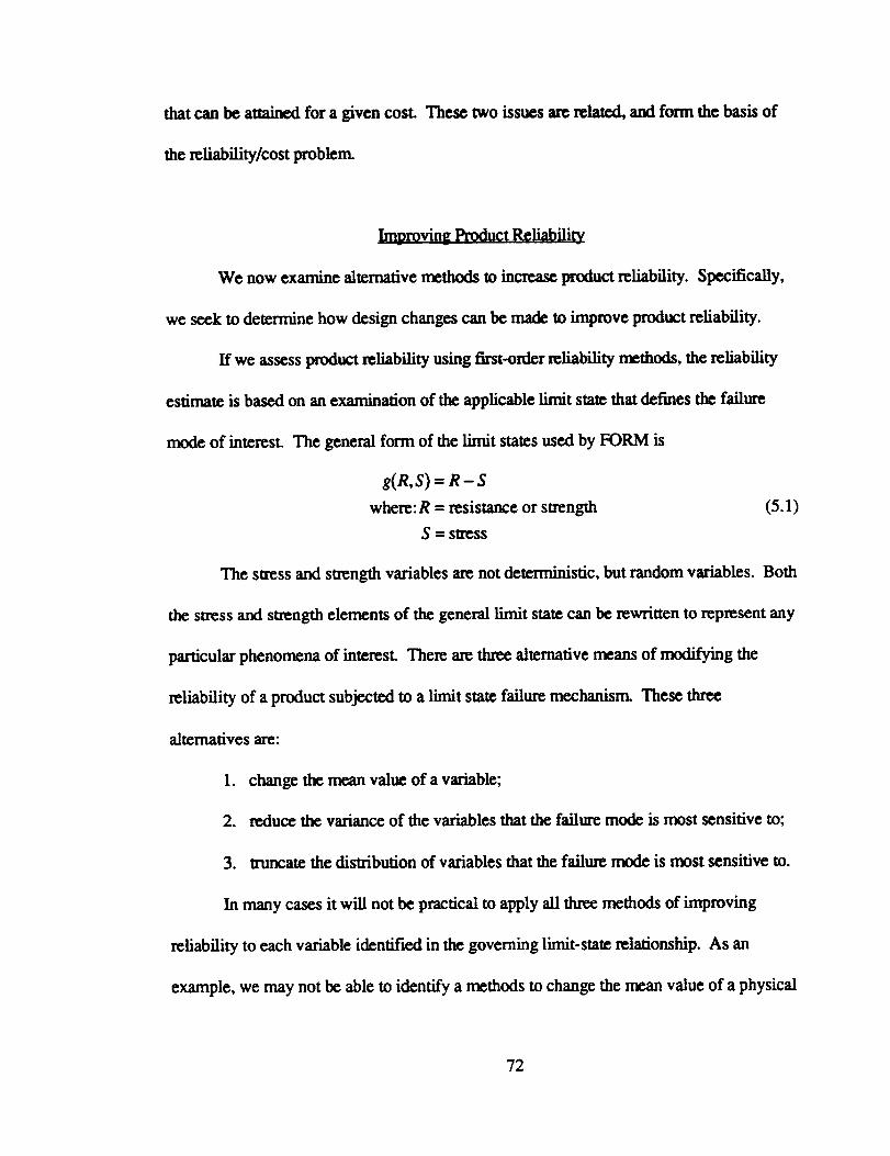
that can be attained for a given cost.
the reliability/cost problem.
These two issues are related, and form the basis of
Improving Product Reliability_
We now examine alternative methods to increase product reliability. Specifically,
we seek to determine how design changes can be made to improve product reliability.
If we assess product reliability using first-order reliability methods, the reliability
estimate is based on an examination of the applicable limit state that defines the failure
mode of interest. The general form of the limit states used by FORM is
g(R,S) = R- S
where: R = resistance or strength (5.1)
S = StreSS
The stress and strength variables are not deterministic, but random variables. Both
the stress and strength elements of the general limit state can be rewritten to represent any
particular phenomena of interest. There are three alternative means of modifying the
reliability of a product subjected to a limit state failure mechanism. These three
alternatives are:
1. change the mean value of a variable,
2. reduce the variance of the variables that the failure mode is most sensitive to;
3. U'uncate the distribution of variables that the failure mode is most sensitive to.
In many cases it will not be practical to apply all three methods of improving
reliability to each variable identified in the governing limit-state relationship. As an
example, we may not be able to identify a methods to change the mean value of a physical
72
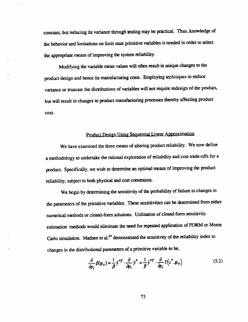
constant, but reducing its variance through testing may be practical. Thus, knowledge of
the behavior and limitations on limit state primitive variables is needed in order to select
the appropriate means of improving the system reliability.
Modifying the variable mean values will often result in unique changes to the
product design and hence its manufacturing costs. Employing techniques to reduce
variance or mmcate the distributions of variables will not require redesign of the product,
but will result in changes to product manufacturing processes thereby affecting product
COSL
Product Design Using Sequential Linear A_vproximation
We have examined the three means of altering product reliability. We now define
a methodology to undertake the rational exploration of reliability and cost trade-offs for a
product. Specifically, we wish to determine an optimal means of improving the product
reliability, subject to both physical and cost constraints.
We begin by determining the sensitivity of the probability of failure to changes in
the parameters of the primitive variables. These sensitivities can be determined from either
numerical methods or closed-form solutions. U_zation of closed-form sensitivity
estimation methods would eliminate the need for repeated application of FORM or Monte
Carlo simulation. Madsen et al._ demonstrated the sensitivity of the reliability index to
changes in the distributional parameters of a primitive variable to be,
1 -*T o3 * (5.2)
73
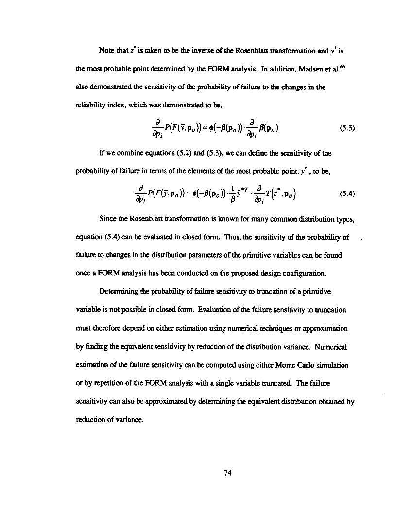
Note that z" is taken to be the inverse of the Rosenblatt transformation and y" is
the most probable point determined by the FORM analysis. In addition, Madsen et aL_
also demonstrated the sensitivity of the probability of failure to the changes in the
reliability index, which was demonstrated to be,
If we combine equations (5.2) and (5.3), we can define the sensitivity of the
probability of failure in terms of the elements of the most probable point, y", to be,
1 -*Y _3 ,
-_ii P(F(y, Po )) -" O(-_(Po ))'_Y ""_ii T( z ,Po) (5.4)
Since the Rosenblatt transformation is known for many common distribution types,
equation (5.4) can be evaluated in closed form. Thus, the sensitivity of the probability of
failure to changes in the dislribufion parameters of the primitive variables can be found
once a FORM analysis has been conducted on the proposed design configuration.
Determining the probability of failure sensitivity to truncation of a primitive
variable is not possible in closed form. Evaluation of the failure sensitivity to truncation
must therefore depend on either estimation using numerical techniques or approximation
by finding the equivalent sensitivity by reduction of the distribution variance. Numerical
estimation of the failure sensitivity can be computed using either Monte Carlo simulation
or by repetition of the FORM analysis with a single variable truncated. The failure
sensitivity can also be approximated by determining the equivalent distribution obtained by
reduction of variance.
74
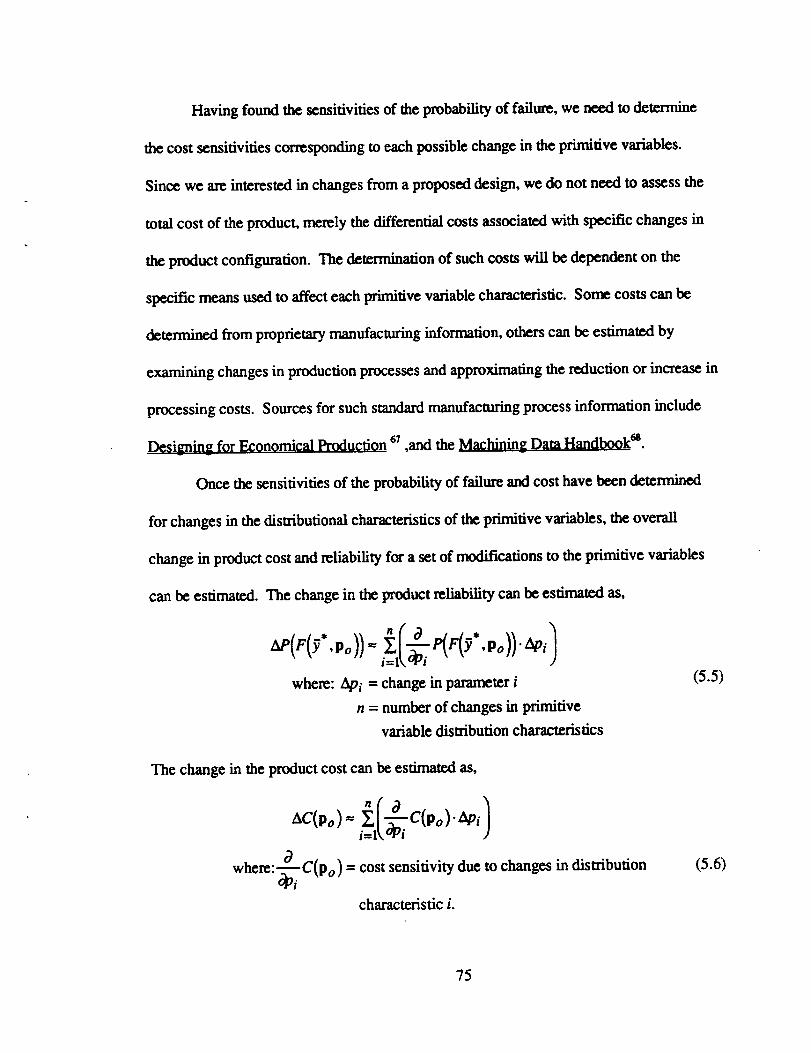
Havingfound the sensitivities of the probability of failure, we need to determine
the cost sensitivities corresponding to each possible change in the primitive variables.
Since we are interested in changes from a proposed design, we do not need to assess the
total cost of the product, merely the differential costs associated with specific changes in
the product configuration. The determination of such costs will be dependent on the
specific means used to affect each primitive variable characteristic. Some costs can be
determined from proprietary manufacturing information, others can be estimated by
examining changes in production processes and approximating the reduction or increase in
processing costs. Sources for such standard manufacturing process information include
Desiring for Economical Production 67 ,and the Mschining Data Handbook _.
Once the sensitivities of the probability of failure and cost have been determined
for changes in the distributional characteristics of the primitive variables, the overall
change in product cost and reliability for a set of modifications to the primitive variables
can be estimated. The change in the product reliability can be estimated as,
where: _i - change in parameter i (5.5)
n = number of changes in primitive
variable distribution characteristics
The change in the product cost can be estimated as,
Ac( o)= C(po). ii=l\_'Yi
where:_-_-C(Po) = cost sensitivity due to changes in distribution (5.6)
characteristic i.
75
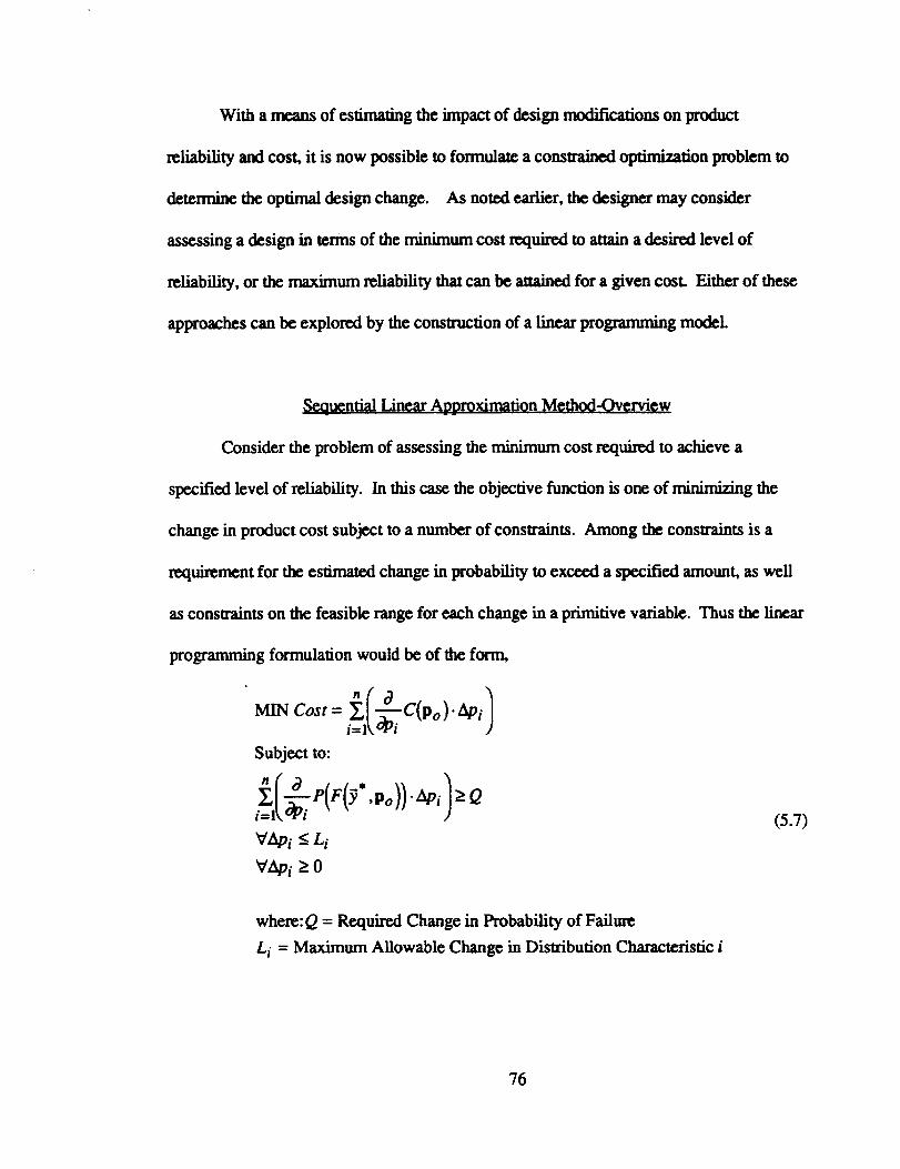
With a means of estimating the impact of design nxxlWw, ations on product
reliability and cost, it is now possible to formulae a constrained optimization problem to
determine the optimal design change. As noted earlier, the designer may consider
assessing a design in terms of the minimum cost required to attain a desired level of
reliability, or the maximum reliability that can be attained for a given cost. Either of these
approaches can be explored by the construction of a linear programming modeL
S_ucntial Linear Approximation Method-Overview
Consider the problem of assessing the minimum cost required to achieve a
specified level of reliability. In this case the objective function is one of minimizing the
change in product cost subject to a number of constraints. Among the constraints is a
requirement for the estimated change in probability to exceed a specified amount, as well
as constraints on the feasible range for each change in a primitive variable. Thus the linear
programming formulation would be of the form,
Co t=
Subject to:
VApi < L i
VAp_ > 0
where:Q = Required Change in Probability of Failure
L i = Maximum Allowable Change in Distribution Characteristic i
76
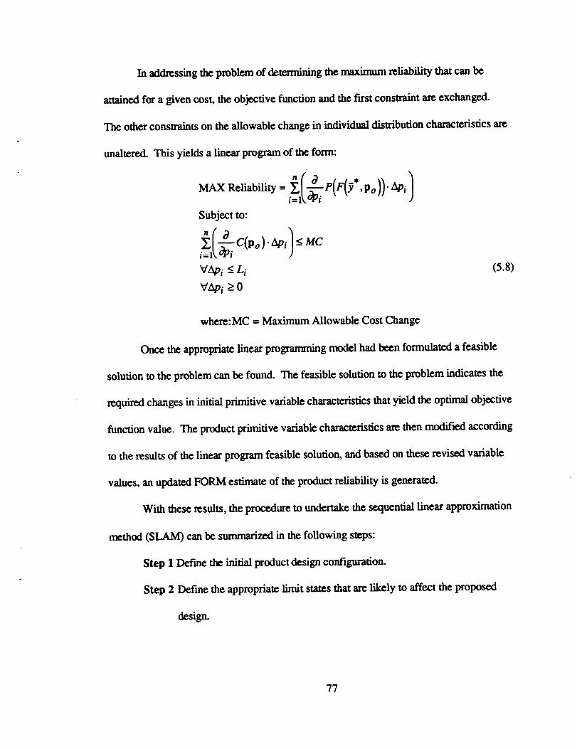
In addressingtheproblem ofdeterminingthemaximum reliabilitythatcan be
attainedfora given cost,theobjectivefunctionand thefirstconswaintare exchanged.
The otherconstraintson the allowablechange inindividualdistributioncharacteristicsare
unaltered.This yieldsa linearprogram of theform:
n 0 --*
Subject to:
£ ['--c.po). -.MCi=l_.O_i
VApi < Li (5.8)
Vtp i ___0
where:MC = Maximum Allowable Cost Change
Once the appropriate linear programming model had been formulated a feasible
solution to the problem can be found. The feasible solution to the problem indicates the
required changes in initial primitive variable characteristics that yield the optimal objective
function value. The product primitive variable characteristics are then modified according
to the results of the linear program feasible solution, and based on these revised variable
values, an updated FORM estimate of the product reliability is generated.
With these resdts, the procedure to undertake the sequential linear approximation
method (SLAM) can be summarized in the following steps:
Step 1 Define the initial product design configuration.
Step 2 I)efme the appropriate limit states that are likely to affect the proposed
design.
77
Step 3 Constructa pexmissibilitymatrixwhich identifiesthefeasiblechanges inthe
disuibution characteristics of every primitive variable in the limit state.
Step 4 Use FORM to estimate the probability of failure, P(F), and the most
probable point,y'. Iftheprobabilityoffailuremeets performance
sw.cifications,stop;otherwisecontinue tostep5.
Step $ Calculatetheprobabilityof failuresensitivities,OP(F)/Opi,forthefeasible
changes indistributioncharacteristicsofevery primitivevariable.
Step 6 Calculatethecostsensitivities,OC/Op_, forthe feasiblechanges in
distributioncharacteristicsof every prirnitivcvariable.
Step 7 Formulate thelinearprogramming model required.
Step 8 Use theLinearprogram todeterminethe requiredchanges inprimitive
variabledistributioncharacteristics,Api. Using theestimatedchanges in
distributioncharacteristicsfound instep8,returntostep4,and update the
estimated product reliability.
A flowchart detailing the methodology enumerated above is presented in Figure 12.
78
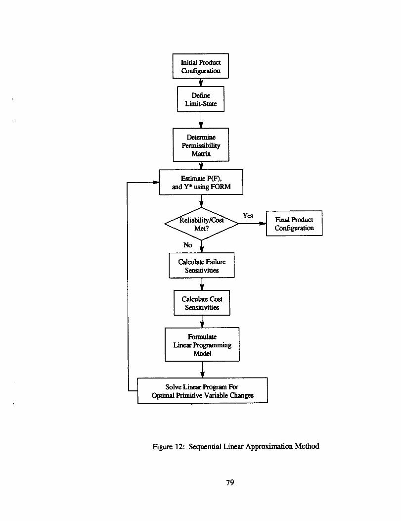
r
Initial Product [Configuration
V
DefineLimit-State
Pe_ibility
EstimateP(F),and Y* using FORM
I Calculate FailureSe_itivities
Calcula_ Cost ISensitivities
F_rmul_
Linca Programming
Model
SolveLinearProgram For
OptimalPrimitiveVariableChanges
VanalProduct
Configuration
Figure 12: Sequential Linear Approximation Method
79
Applying the Sequential Linear Avproximation Method
We now demonstrate the application of the sequential linear approximation
method by way of example. Consider the design of a water pump for a large stationary
emergency diesel generator. The unit is an 8 cylinder, 4-cycle diesel engine rated at 3500
kW, operating at 450 rpm. From analysis of the engine cooling needs, approximately 800
gpm of coolant water will be required during engine operation. Based on shear stress and
allowable torsional twist, the water pump shaft should be at least 1.5 inches in diameter
and 12 inches long. The pump rotates at 300 rpm and drives an 8 inch diameter steel
impeller. The shaft rotates in a solid bushing bearing. The allowable wear on the shaft
after 2 years of operation must not exceed 0.007 inches in order to maintain acceptable
alignment of the drive gear train. We are interested in examining the pump design to
demonstrate how to attain a desired reliability for minimum cost, as well as how much
improvement in reliability can be attained for a fixed cost level.
The initial pump shaft design parameters are presented below.
8O
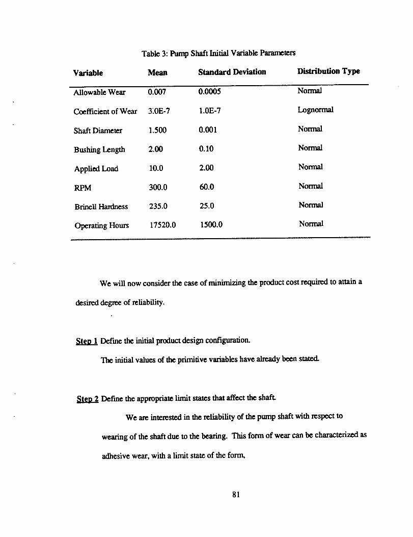
Variable
Table 3: Pump Shaft Initial Variable Parameters
Mean Standard Deviation Distribution Type
Allowable Wear 0.007 0.0005 Normal
Coefficient of Wear 3.0E-7 1.0E-7 Lognormal
Shaft Diameter 1.500 0.001 Normal
Bushing Length 2.00 0.10 Normal
Applied Load 10.0 2.00 Normal
RPM 300.0 60.0 Normal
BrineU Hardness 235.0 25.0 Normal
Operating Hours 17520.0 1500.0 Normal
We will now consider the case of minimizing the product cost required to attain a
desired degree of reliability.
Steel Define the initial product design configuration.
The initial values of the primitive variables have already been stated.
Step2 Define the appropriate limit states that affect the shall
We are interested in the reliability of the pump shaft with respect to
wearing of the shaft due to the bearing. This form of wear can be characterized as
adhesive wear, with a limit state of the form,
81
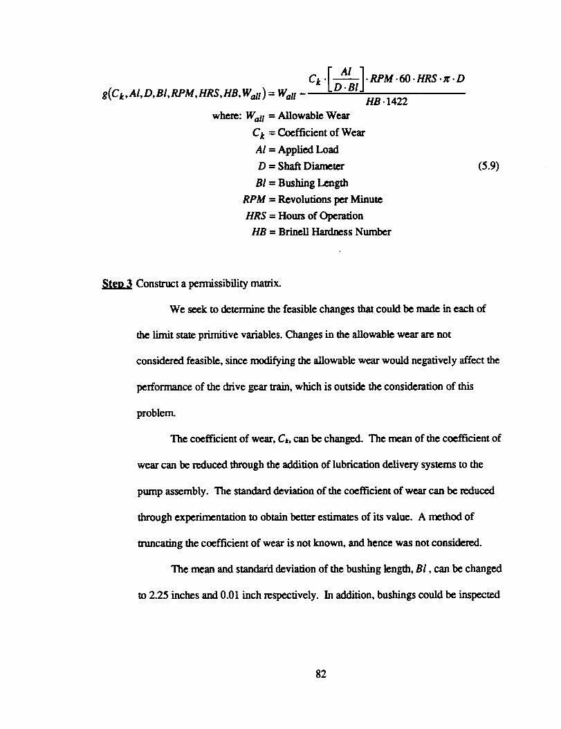
g(Ck,AI, D, BI, RPM, HRS,HB, Wall) = Wai i
c,.r ]. .,Rs.,,.LD.BIJ
liB. 1422
where: Wal I = Allowable Wear
Ck
Al
D
Bl
RPM
HRS
lib
= Coefficient of Wear
= Applied Load
= Shaft Diameter
= Bushing Length
= Revolutions per Minute
= Hours of Operation
= Brinell Hardness Number
(5.9)
Stev3 Construct a permissibility matrix.
We seek to determine the feasible changes that could be made in each of
the limit state primitive variables. Changes in the allowable wear are not
considered feasible, since modifying the allowable wear would negatively affect the
performance of the drive gear train, which is outside the consideration of this
problem.
The coefficient of wear, C,, can be changed. The mean of the coefficient of
wear can be reduced through the addition of lubrication delivery systems to the
pump assembly. The standard deviation of the coefficient of wear can be reduced
through experimentation to obtain better estimates of its value. A method of
truncating the coefficient of wear is not known, and hence was not considered.
The mean and standaht deviation of the bushing length, Bl, can be changed
to 2.25 inches and 0.01 inch respectively. In addition, bushings could be inspected
82
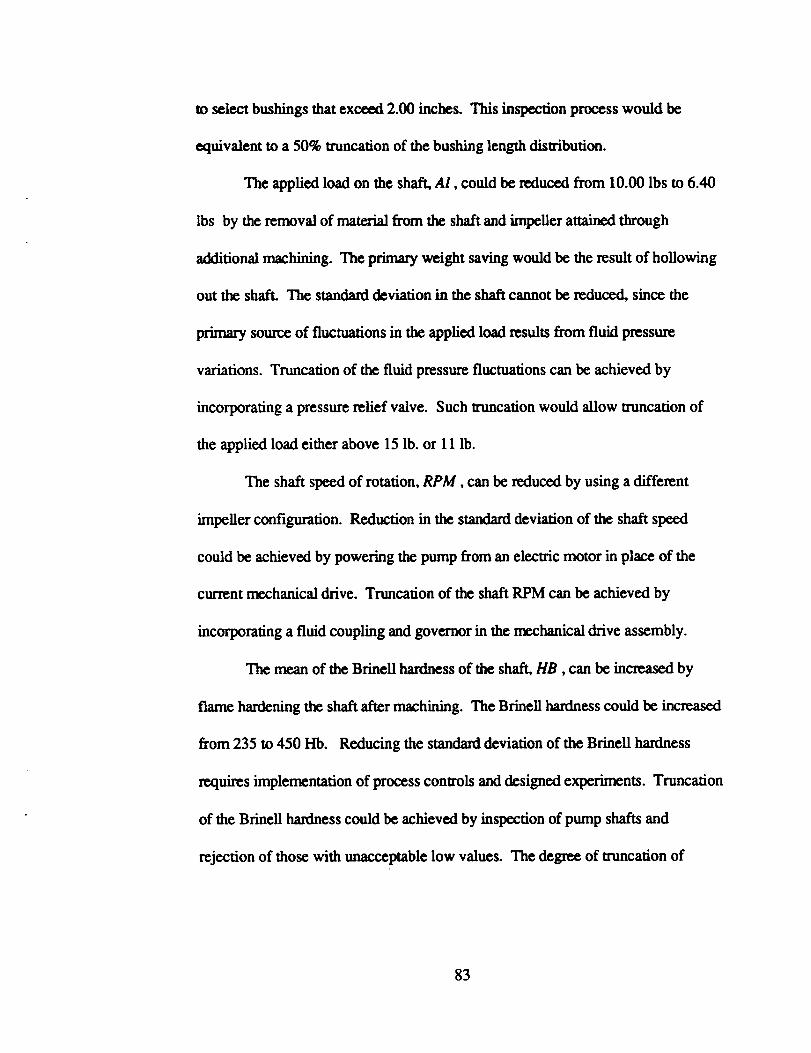
to select bushings that exceed 2.00 inches. This inspection process would be
equivalent to a 50% u'uncation of the bushing length distribution.
The appLied load on the shaft, Al, could be reduced from 10.00 lbs to 6.40
lbs by the removal of material from the shaft and impeller attained through
additional machining. The primary weight saving would he the result of hollowing
out the shaft. The standard deviation in the shaft cannot be reduced, since the
primary source of fluctuations in the appLied load results from fluid pressure
variations. Truncation of the fluid pressure fluctuations can be achieved by
incorporating a pressure relief valve. Such truncation would allow truncation of
the applied load either above 15 lb. or 11 lb.
The shaft speed of rotation, RPM, can be reduced by using a different
impeller configuration. Reduction in the standard deviation of the shaft speed
could be achieved by powering the pump from an electric motor in place of the
current mechanical drive. Truncation of the shaft RPM can be achieved by
incorporating a fluid coupling and governor in the mechanical drive assembly.
The mean of the Brinell hardness of the shaft, liB, can be increased by
flame hardening the shaft after machining. The Brinell hardness could be increased
from 235 to 450 Hb. Reducing the standard deviation of the Brinell hardness
requires implementation of process controls and designed experiments. Truncation
of the Brinell hardness could he achieved by inspection of pump shafts and
rejection of those with unacceptable low values. The degree of truncation of
83
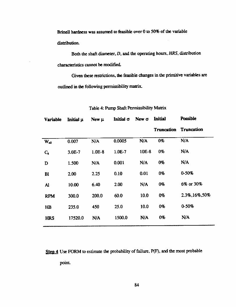
Brinell hardnesswasassumed to feasible over 0 to 50% of the variable
distribution.
Both the shaft diameter, D, and the operating hours, HRS, distribution
characteristics cannot be modified.
Given these restrictions, the feasible changes in the primitive variables are
outlined in the following permissibility matrix.
Variable Initial I_
Table 4: Pump Shaft Permissibility Mau'ix
New I.t Initial a New o Initial
Truncation
Possible
Truncation
W,n 0.007 N/A 0.0005 N/A 0% N/A
C_ 3.0E-7 1.0E-8 1.0E-7 10E-8 0% N/A
D 1.500 N/A 0.001 N/A 0% N/A
131 2.00 2.25 0.10 0.01 0% 0-50%
AI 10.00 6.40 2.00 N/A 0% 6% or 30%
RPM 300.0 200.0 60.0 10.0 0% 2.3%,16%,50%
HB 235.0 450 25.0 10.0 0% 0-50%
HRS 17520.0 N/A 1500.0 N/A 0% N/A
Stea4 Use FORM to estimate the probability of failure, P(F), and the most probable
point.
84
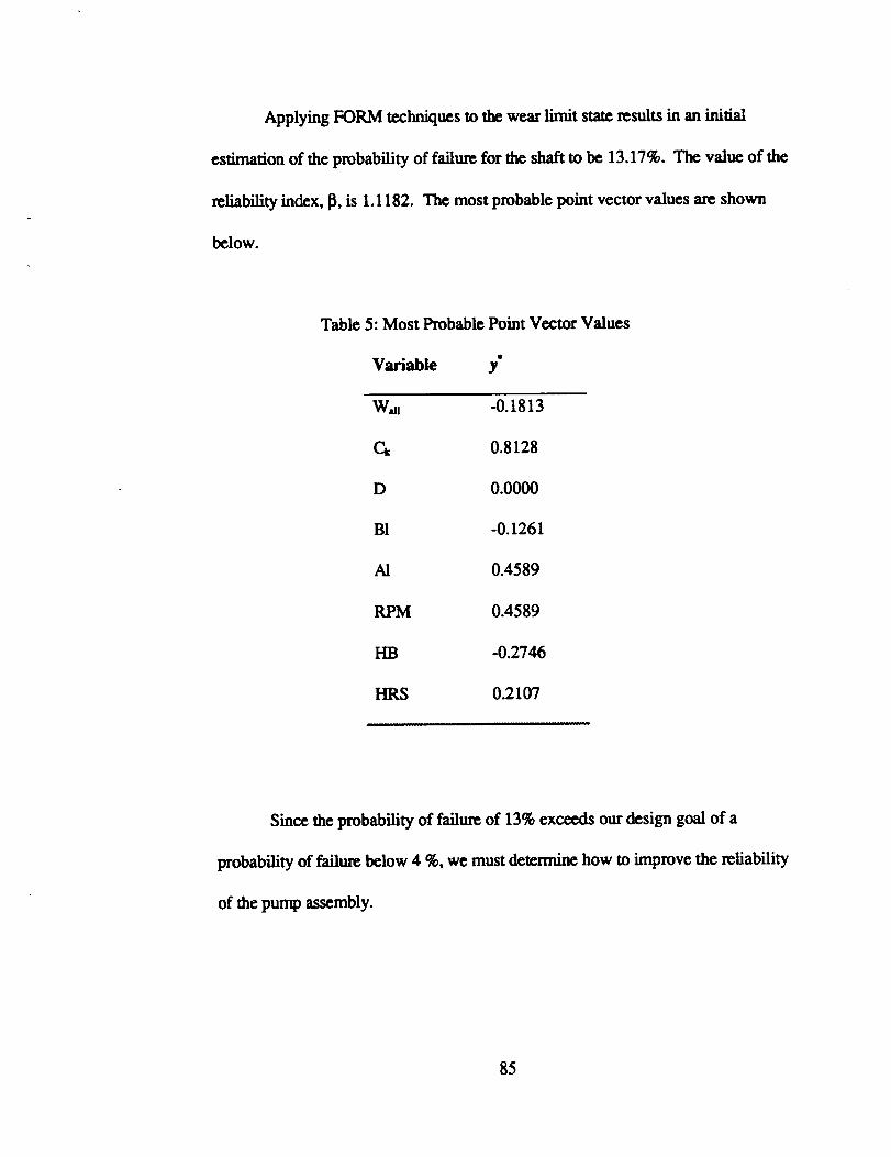
Applying FORM techniques to the wear limit state results in an initial
es1L,nation of the probability of failure for the shaft to be 13.17%. The value of the
reliability index, 13, is 1.1182. The most probable point vector values are shown
below.
Table 5: Most Probable Point Vector Values
g
Variable y
W_ -0.1813
C_ 0.8128
D 0.0000
131 -0.1261
AI 0.4589
RPM 0.4589
HB -0.2746
HRS 0.2107
Since theprobabilityof failureof 13% exceeds our designgoalof a
probabilityoffailurebelow 4 %, we must determinehow toimprove the reliability
of thepump assembly.
85
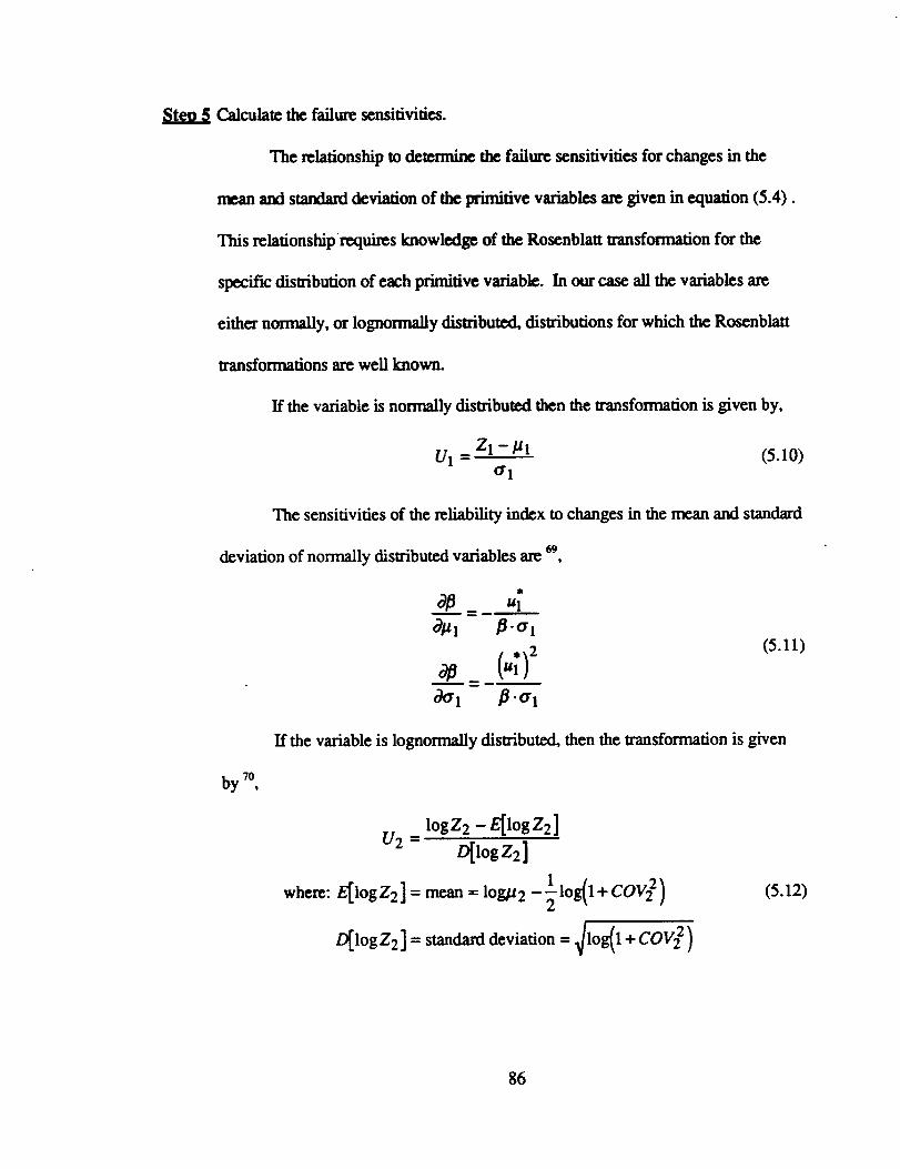
Steo5 Calculate the failure sensitivities.
The relationship to determine the failure sensitivities for changes in the
mean and standard deviation of _e primitive variables are given in equation (5.4).
This relationship requires knowledge of the Rosenblau transformation for the
specific dis_bution of each primitive variable. In our ease all the variables are
either normally, or lognormally disu'ibuted, distributions for which the Rosenblatt
wansformafions are well known.
If the variable is normally distributed then the wansformation is given by,
U l = Zt -_ut (5.10)al
The sensitivities of the reliability index to changes in the mean and standard
deviation of normally distributed variables are 69,
o_fl u 1
0_1 fl .o l
Oal fl .ol
by 7o
(5.11)
If the variable is lognormally distributed, then the wansformation is given
logz -E[logZ ]O[logZz]
w.o : = -1,o O+Cov )D[logZ2] = standarddeviation=7log(1 +COV 2)
(5.12)
86
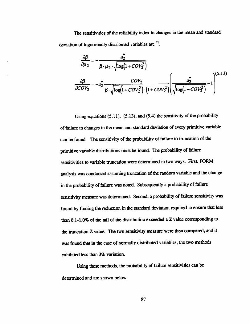
The sensitivities of the reliability index to changes in the mean and standard
deviation of lognonmUy distributed variables am 71,
d/_ u2
/4 "• COV 2 u2
o- 2 -0÷ (5.13)
Using equations (5.11), (5.13), and (5.4) the sensitivity of the probability
of failure to changes in the mean and standard deviation of every primitive variable
can be found. The sensitivity of the probability of failure to truncation of the
primitive variable distributions must be found. The probability of failure
sensitivities to variable truncation were determined in two ways. First, FORM
analysis was conducted assuming truncation of the random variable and the change
in the probability of failure was noted. Subsequently a probability of failure
sensitivity measure was determined. Second, a probability of failure sensitivity was
found by finding the reduction in the standard deviation required to ensure that less
than 0.1-1.0% of the tail of the distribution exceeded a Z value corresponding to
the truncation Z value. The two _nsitivity measure were then compared, and it
was found that in the case of normally distributed variables, the two methods
exhibited less than 3% variation.
Using these methods, the probability of failure sensitivities can be
determined and are shown below.
87
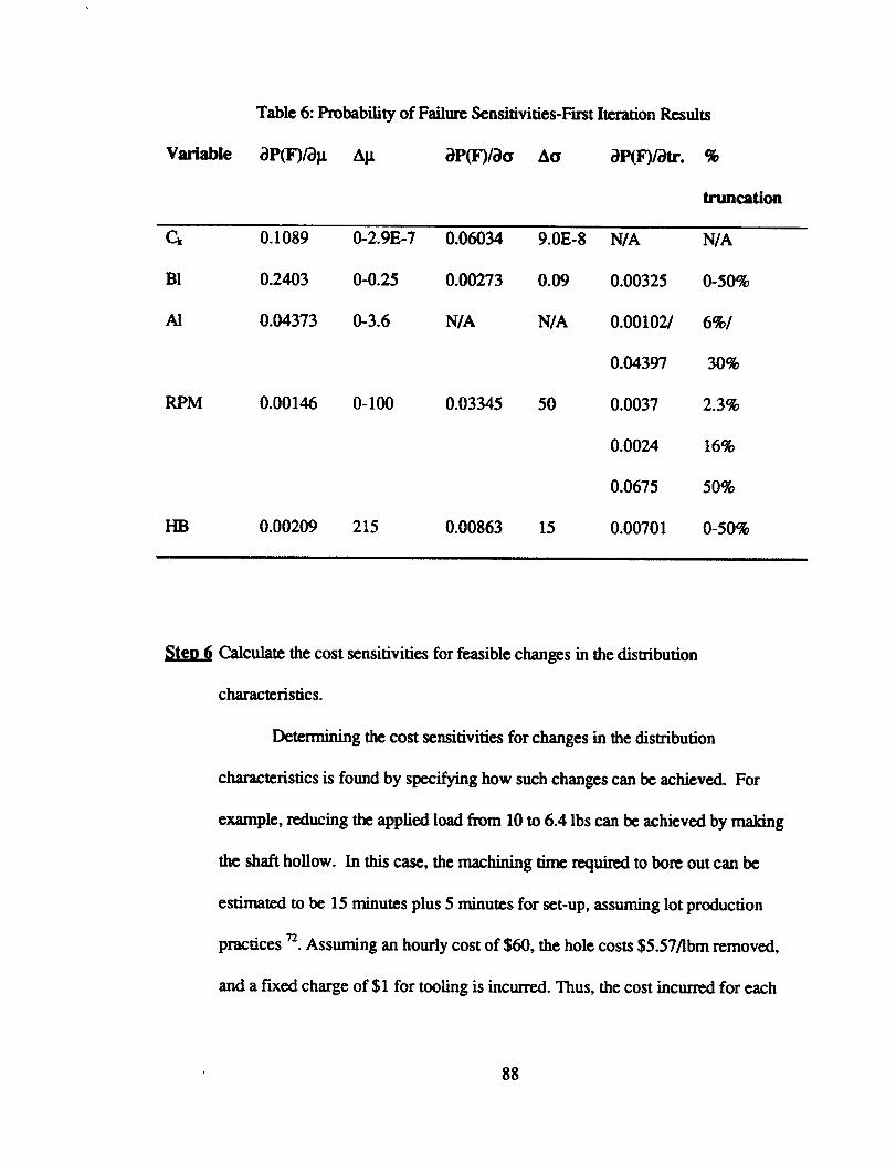
Variable
Table 6: Probability of Failure Sensitivities-Ftrst Iteration Restflts
0P(F)/_g Ag BP(F)/ao Ao BP(10/'Otr. %
truncation
0.1089 0-2.9E-7 0.06034 9.0E-8 N/A N/A
B1 0.2403 0-0.25 0.00273 0.09 0.00325 0-50%
A1 0.04373 0-3.6 N/A N/A 0.00102/ 6%1
0.04397 30%
RPM 0.00146 0-100 0.03345 50 0.0037 2.3%
0.0024 16%
0.0675 50%
HB 0.00209 215 0.00863 15 0.00701 0-50%
Stea6 Calculate the cost sensitivities for feasible changes in the distribution
characteristics.
Determining the cost sensitivities for changes in the distribution
characteristics is found by specifying how such changes can be achieved. For
example, reducing the applied load from 10 to 6.4 lbs can be achieved by making
the shaft hollow. In this case, the machining time required to bore out can be
estimated to be 15 minutes plus 5 minutes for set-up, assuming lot production
practices 72. Assuming an hourly cost of $60, the hole costs $5.57/lbm removed,
and a fixed charge of $1 for tooling is incurred. Thus, the cost incmred for each
88
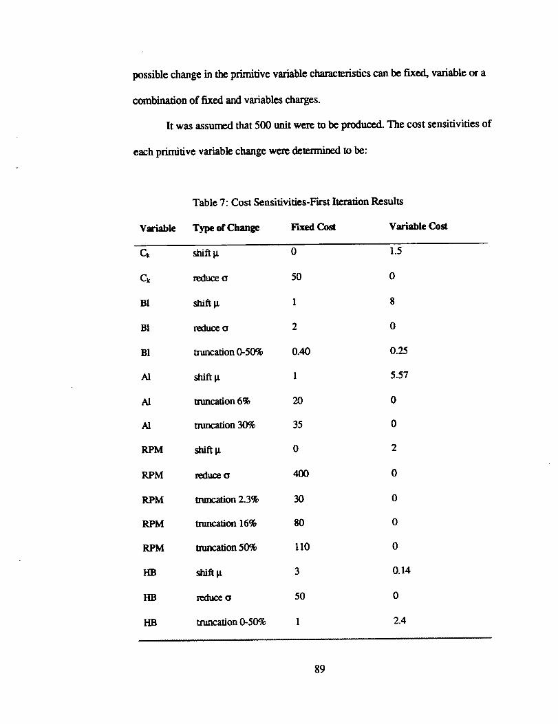
possiblechange in the primitive variable characteristics can be fixed, variable or a
combination of fixed and variables charges.
It was assumed that 500 unit were to be produced. The cost sensitivities of
each primitive variable change were determined to be:
Variable
Table 7: Cost Sensitivities-First Iteration Results
Type of Change F'u_ed Cost Variable Cost
Ck shift St 0 1.5
Ck reduce a 50 0
B1 shift St 1 8
BI rexlu_ a 2 0
BI truncation 0-50% 0.40 0.25
A1 shift St 1 5.57
A1 mmcation 6% 20 0
A1 mmcation 30% 35 0
RPM shift St 0 2
RPM reduce a 400 0
RIM tnmcation 2.3% 30 0
RIM truncation 16% 80 0
RPM ffuncafion 50% 110 0
IIB shift St 3 0.14
HB reduce o 50 0
I-IB truncation 0-50% 1 2.4
89
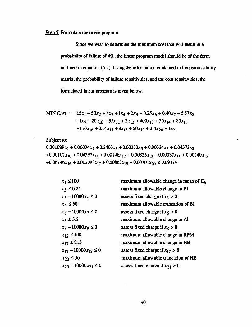
Step7 Formulate the linear program.
Since we wish to determine the minimum cost that will result in a
probability of failure of 4%, the linear program model should be of the form
outlined in equation (5.7). Using the information contained in the permissibility
matrix, the probability of failure sensitivities, and the cost sensitivities, the
formulated linear program is given below.
MIN Cost = 1.5x I + 50x 2 + 8x 3 + IX 4 + 2X 5 + 0.25X 6 + 0.40X 7 + 5.57X8
+lx9 + 20X10 + 35Xl I + 2X12 + 400X13 + 30X14 + 80X15
+110X16 + 0.14X17 + 3X18 + 50X19 + 2.4X20 + lx21
Subjectto:
0.001089xI + 0.06034x2 + 0.2403x3 + 0.00273x5 + 0.00324x 6 + O.IM373x$
+O.O0102xlo + 0.04397xii+ 0.00146x12 + 0.00335x13 + 0.00037x14 + 0.00240x15
+0.06746x16 + 0.002093x17 + 0.00863x19 + 0.00701x2o __.0.09174
x 1 < 100
x 3 < 0.25
x 3 - 10000x 4 < 0
x 6 < 50
x 6 - 10000x 7 < 0
x 8 < 3.6
x 8 - 10000x 9 < 0
x12 < 100
x17 _<215
x17 - 10000x18 < 0
x20 < 50
x20 - 10000x21 < 0
maximum allowable change in mean of C k
maximum allowable change in B1
assess fixed charge ifx 3 > 0
maximum allowable truncation of BI
assess fixed charge ifx 6 > 0
maximum allowable change in AI
assess fixed charge ifx 8 > 0
maximum allowable change in RPM
maximum allowable change in liB
assess fixed charge ifxl7 > 0
maximum allowable truncation of liB
assess fixed charge if x21 > 0
90
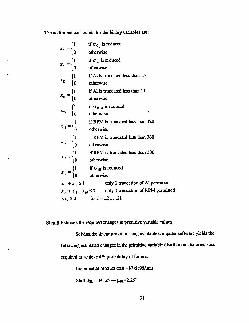
Theadditionalconstraintsfor the binary variables are:
. :{10, :{'0XI° = {10
Xt| - {10
X13 = {10
Xl 4 "-- {10
X15 = 0
Xl6 = {10
XI9 -- {I0
at0 + all
x14'+ x15
Vx_ > 0
if Oc_ is reduced
otherwise
if OB_ is reduced
otherwise
if AI is truncated less than 15
otherwise
if Al is tnmcated less than 11
otherwise
if O_M is reduced
othe_
if RPM is truncated less than 420
otherwise
if RPM is truncated less than 360
otherwise
if RPM is truncated less than 300
otherwise
if o_ is reduced
otherwise
_<1 only 1 truncation of AI permitted
+ xt6 < 1 only 1 u'uncation of RPM permitted
for i = 1,2,...,21
Ste¢8 Estimate the required changes in primitive variable values.
Solving the linear program using available computer software yields the
following estimated changes in the primitive variable distribution characteristics
required to achieve 4% probability of failure.
Incremental product cost =$7.6195/unit
Shift _tBL= +0.25 --->_tBL=2.25"
91
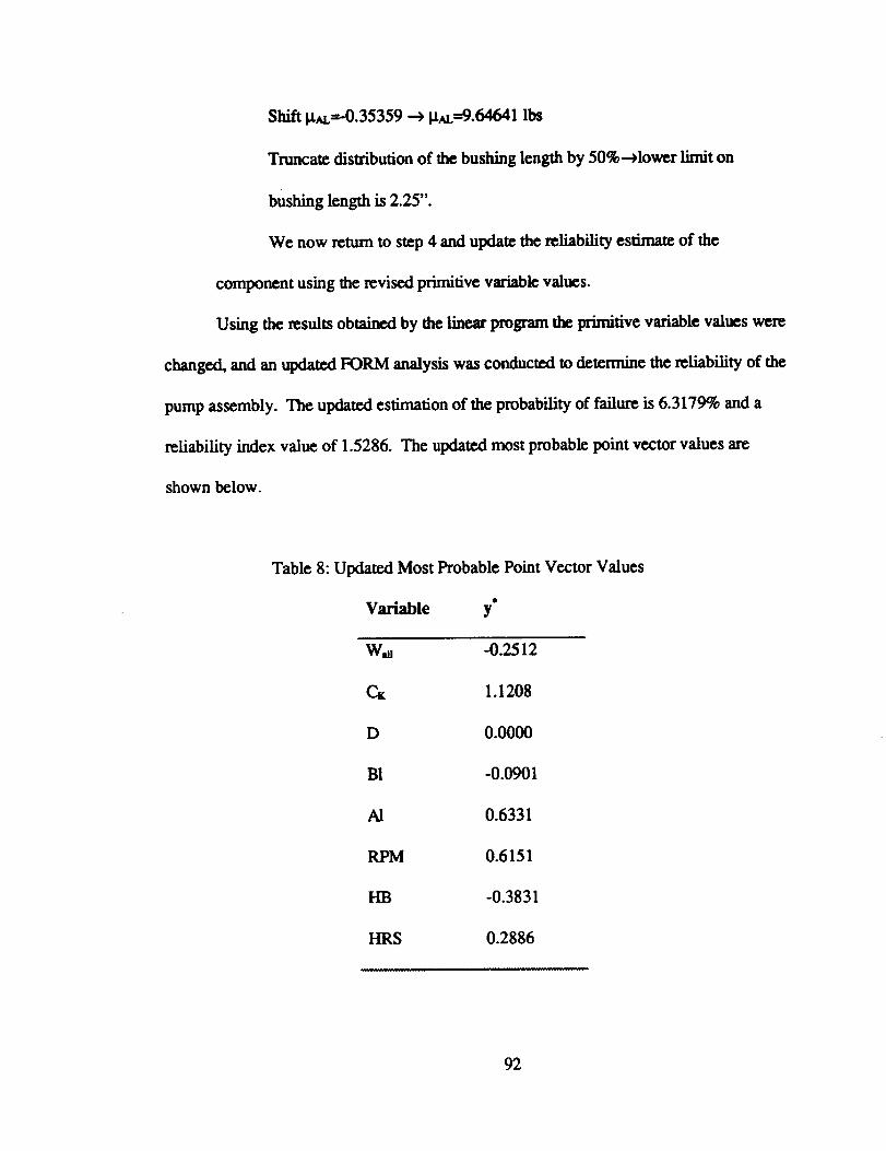
Shift I.t_L=-0.35359 --_ IX_----'9.64641 lbs
Truncate disu'ibution of the bushing length by 50%--_lower limit on
bushing length is 2.25".
We now return to step 4 and update the reliability estimate of the
component using the revised primitive variable values.
Using the results ob_ned by the linear program the primitive variable values were
changed, and an updated FORM analysis was conducted to determine the reliability of the
pump assembly. The updated estimation of the probability of failure is 6.3179% and a
reliability index value of 1.5286. The updated most probable point vector values are
shown below.
Table 8: Updated Most Probable Point Vector Values
o
Variable y
W_ -0.2512
CK 1.1208
D 0.0000
BI -0.0901
AI 0.6331
RPM 0.6151
HB -0.3831
HRS 0.2886
92
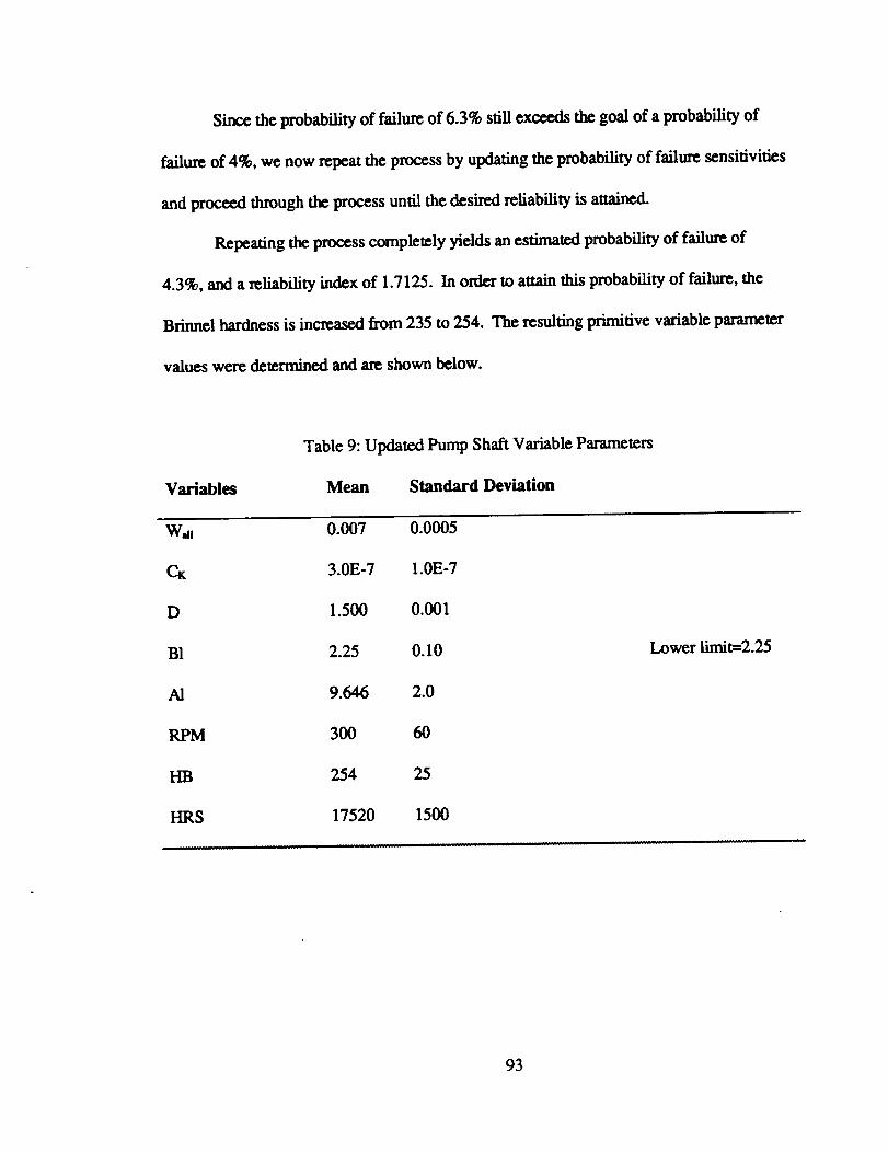
Sincethe probability of failure of 6.3% still exceeds the goal of a probability of
failure of 4%, we now repeat the process by updating the probability of failure sensitivities
and proceed through the process until the desired reliability is attained.
Repeating the process completely yields an estimated probability of failure of
4.3%, and a reliability index of 1.7125. In order to attain this probability of failure, the
Brinnel hardness is increased f_om 235 to 254. The resulting primitive variable parameter
values were determined and are shown below.
Variables
Table 9: Updated Pump Shaft Variable Parameters
Mean Standard Deviation
W_ 0.007 0.0005
Ct 3.0E-7 1.0E-7
D 1.500 0.001
B1 2.25 0.10
A1 9.646 2.0
RIM 300 60
HB 254 25
HRS 17520 1500
Lower limit=2.25
93
The overall cost associated with these changes in the primitive variables is
estimated to be $13.232Amit. Additional repetition of the process would yield a probability
of failure less than 4%.
In considering the case of the maximizing the product reliability for a given
increase in cost, the procedure is identical with the exception of the formulation of the
linear programming model. In this case, the reliability constraint becomes the objective
function, and the previous cost minimization objective function becomes a consu'aint. The
determination of the coefficients for reliability maximi_tion is accomplished in the same
manner as outlined.
When the reliability maximization problem is considered for the pump shaft
problem restricted to a maximum allowable cost increment of $7.62, the resulting changes
in the primitive variable distributional characteristics are identical to those found for the
cost minimization case.
Implications of the Seouential Linear Agproximation Methodolog'y
Having defined and demonswated the sequential linear approximation
methodology, two implications are evident. First the application of the proposed
methodology will permit the designer/engineer to rationally explore the trade-off between
component reliability and cost. More importandy, the designer will be provided with
information as to the optimal means 0f improving a proposed design, with respect to either
cost or reliability. The ability to directly link reliability and cost of proposed product
94

designs provides management with the ability to directly treasure the impact of changes in
a design on product costs.
The second implication of the methodology is that it provides designers and
management with a rapid means of assessing the potential reliability of competing designs.
By investigating a proposed design and focusing on the maximum reliability attainable for
a specified cost increase, management can evaluate differing alternative designs to
determine those designs that offer the greatest potential for improvement.
These two benefits provide mangers and engineers with more useful information
regarding product cost and reliability than alternative design methodologies.
95
CHAFFERVI
CONCLUSIONS AND FUTURE RESEARCH
We have developed a design rr_thodology that allows engineers to undertake
reliability and cost trade-off analysis. We have shown how current analytical reliability
methods cannot be incorporated into the design methodology due to four limitations on
their use. First, the absence of physical variables in analytical methods was shown to
prevent their use in the assessment of variable changes on reliability. Second, analytical
reliability methods were shown not to include the unique operating conditions experience
by the component in the reliability estimates. Third, the restriction of analytical reliability
methods to the estimation of systems that have attained steady-state failure ram conditions
was demonstrated. The time to attain steady state failure rates was shown to be several
time greater than the component MTTF, indicating the need to be able to estimate
component reliability during this operating time. Fourth, analytical reliability methods
were shown not to consider the impact of variance reduction on reliability and cost.
These four limitations precluded the use of analytical methods in reliability-cost trade-off
methodology.
We have demonstrated the feasibility and validity of extending FORM to
mechanical system design. We demonstrated thateven atlow probabilitiesoffailure
FORM and Monte Carlo yieldmarkedly similarresults.We detailedhow FORM provides
96
one of two major elements needed in the design paradigm by providing a means of
estimating reliability sensitivity to primitive variable distributional changes. We examined
how FORM represents a less restrictive reliability methodology since it can be applied to
systems that are unique, as well as being valid for the reliability assessment of a system in
either steady-state or transient failure rate regimes.
We showed that although the physics-based failure rate reliability method provides
for the assessment of the impact of changes in the primitive variable on component
reliability, it has several limitations. Physics-based failure rate methods were demonstrated
to involve changes in the mean of primitive variables, and consequently, does not allow for
the estimation of the impact of variance reduction on component reliability. The reliance
of physics-based methods on base failure rates was shown to restrict its application to
components with design and operating conditions similar to existing components.
We proved that the base failure rates used by the physics-based failure rate method
have a large degree of uncertainty, and that such uncertainty will result in inaccurate
reliability estimates. We demonstrated that the uncertainty in the base failure rates
exceeds the allowable range of change for the primitive variables, making reliability
estimates indistinguishable from the random error of the method. For these reason, the
physics-based failure rate method could not be incorporated in the design trade-off
method.
Finally, we developed the sequential linear approximation method for assessing
component design. We outlined how the method uses reliability and cost to evaluate a
component design. Using the sequential linear approximation method, we have
97
demonstratedhow FORM estimates can be incorporated into the methodology to optimize
product design. The determination of cost sensitivities to changes in primitive variable
distributional parameters, and how such sensitivities are employed by the methodology
was developed. The sequential linear approximation method (SLAM) was demonswa_l
to be an effective means of optimizing the product design with respect to either product
reliability or cost. Using the SLAM approach engineers can determine the optimal means
to improve product design or to assess the ultimate attainable reliability of a proposed
design.
The examination of the existing reliability methods has identified several areas for
future research. First, determination of a mathematical relationship for the transient period
following system comndssioning would provide an assessment tool for new systems.
Second, the lack of information on primitive variable distributions and parameter
values requires substantial basic research. Additional information on the primitive variable
distribution and parameter values would significantly increase the utility of FORM
techniques.
98
APPENDIX A
COMPENDIUM OF MECHANCIAL LIMIT STATES
I. Compendium of Mechanical Limit States
I.I Purpose
The creation of a compendium of mechanical limit states was undertaken in order to
provide a reference base for the application of F'trst-Onter Reliability Methods to
mechanical systems inthecontextof thedevelopment of a system leveldesign
methodology. The compendium was conceived as a referencesource,specifictothe
problem of developing the noted design methodology, and not an exhaustive or exclusive
compilationofmechanical limitstates.The compendium isnot intendedtobe a handbook
of mechanical limitstatesforgeneraluse.
1.2 Proposed Use of Compendium
The compendium provides a diverse set of limit-state relationships for use in
demonslrating the application of probabilistic reliability methods to mechanical systems.
The different limit-state relationships will be used to analyze the reliability of a candidate
mechanical system.
1.3 Selection of Limit-States
In determining the limit-states to be included in the compendium, a comprehensive listing
of thepossiblefailuremodes thatcould affectmechanical systems was generated.
Previous literature defming mechanical modes of failure was studied, and cited failure
modes were included. From this, the following classifications for failure modes were
derived:
-Wear
.Corrosion
-Fatigue
•Material Degradation
With the definition of the differem failure modes, a titeramre search for each was
conducted, with the aim of establishing relationships for each failure mechanism to be used
in formulating mechanical limit-states.
100
The individual failure modes that were determined for each classification are:
Wear
•Adhesive wear
•Abrasive wear
•Lubricated wear
•Fretting wear
•Surface fatigue wear
•Liquid impact erosion
Fatigue
•Low-cycle fatigue
•High-cycle fatigue
•Crack growth
Coffro_on
-Erosion-corrosion
•Galvanic corrosion
•Uniform attack
•Pitting corrosion
.Cavitation
•Crevice corrosion
• Stress corrosion cracking
• Selective leaching
• Inter-granular corrosion
Material Degradation
•Thermal degradation
•Radiation damage
Although it was possible to determine the different failure modes that could affect a
rm.chanical system, the identification of relationships for all noted failure modes was not
possible. The difficulty in identifying some of the limit-state relationships is due to a lack
of accurate analytical models. Consequently, the compendium consists of relationships for
those failure modes for which reasonably robust relationships exist.
1.4 Distribution Properties
The coml_ndium does not contain information on the distribution properties of the
individual primitive variables. With the exception of fatigue and wear related primitive
variables, little research was uncovenxl that dealt with the distribution properties of limit-
state primitive variables. There is significant research available on the best estimates of
variables values, and when appropriate some of these values have been included in the
relevant sections. The lack of much information on the distribution properties of many
primitive variables indicates the need for additional research efforts in this area.
1.5 Form of Limit-State Relationships
The result of the investigation into mechanical fimit-smtes indicate that the vast majority of
identified relationships are of the form of a power law. All the limit states cited within the
compendium, with the exception of those for uniform attack and thermal degradation, take
a power law form.
101

2. Wear
Wear is the removal of material from solid surfaces as a result of mechanical action. In
most cases the amount of the material removed from the surfaces is small in relation to the
ovcraU material mass of the components involved.
Wear processes have been identified to conform to four different forms. The four major
forms of wear enumerate by Rabinowicz (1965) are:
1. Adhesive wear,
2. Abrasive wear;,
3. Corrosive wear,
4. Surface fatigue wear.
In addition to these four major wear processes, there are a number of minor processes that
axe often categorized as being a wear process.
Models for the following wear processes are presented in subsections 1 through 5:
1. Adhesive wear
2. Abrasive wear
3. Lubricated wear
4. Fretting wear
5. Liquid impact erosion.
References
Rabinowicz, E., Friction and Wear of Material, J. Wiley, 1965.
102
2.1 Adhesive Wear
Definition
"Adhesive wear occurs when two smooth bodies are slid over each other, and fragments
are pulled off one surface to adhere to the other" (Rabinowicz, 1965). Once the fragraents
have been tom from their original surface and attached to the opposing surface, they may
reattach to their original surface, or become loose fragments.
Limit-State Formulation
Experimental data indicates that there are three laws of adhesive wear, namely;
o
2.
3.
The amount of wear is generally directly proportional to the load L;
The amount of wear is generally proportional to the distance slid, x;
The amount of wear is generally inversely proportional to the hardness, p,
of the surface being worn away.
Holm (1946) proposed that the volume worn away could be described by:
cLxV-" m
P
where c = material dependent nondimensional constant
Evidence for this relationship is mixed, with some result being very close to the predicted
volumes and other being widely different. Archard (1953) presented a model of sliding
which allows for the derivation of the above equation, while providing insight into the
meaning of the constant, c. From his model we get the following model for the volume of
material worn away through adhesive wear,
103
kLxV- m
where k = coefficient of wear
= probability of any junction
forming a fragment
p = flow pressure of softer metal
As can be seen the difference in these equations is that we have replaced c with k/3. The
only important requirement for the second equation to hold is that the volume of the
fragment should be proportional to the cube of the juncdon diameter.
An alternative form of the second equation is:
V=k_r X
3
where Ar = actual area of contact
Although knowledge of the volume worn is important, typically we are more interested in
the depth of material worn away. The extension of the above relations to yield the depth
of material worn away is given in the W¢_r Comrol Handbook (ASME, 1980);
d KP
L H
where d = depth of wear
P = nominalpressure
L = sliding distance
H = material hardness
104
This form of the wear relationship now pert'nits the estimation of the Life of the surface. If
we let the sliding distance, L, be expressed as the velocity, v, and the time, t, the
relationship becomes:
dH
KPv
The authors go on to demonsWate that the coefficient of wear, K is the proportional of
volume wom away to the theoretical wom volume that would have resulted if every
asperity contact produced a worn particle.
Model Assumptions
The assumptions of the model are:
I. k--probability of any junction forming a fragment
2. Each junction is in existence throughout the sliding distance, d.
Notes
Values for k can be found in Proceedings of the Conference on Lubrication and Wear
(1957 on), and the Transactions of the American Society of Lubrications Engineers (1958-
1963).
References
Rabinowicz, E., Frietign and Wear of Materials, J. Wiley, New York, 1965.
Holm, R., El_tric Contacts, Almquist and Wiksells, Stockholm, 1946.
Archard, J.F., Contact and Rubbing of Flat Surfaces, Journal of Applied Physics, vol. 24,
pp. 981-988.
M.B. Peterson and W.O. Winer, eds., Wear Control Handbook, ASME, New York, 1980.
105
2.2 Abrasive Wear
Definition
Abrasive wear occurs when a rough hard surface, or a soft surface containing hard
particles, slides on a softer surface. As a result of the sliding action, the softer surface has
a series of grooves ploughed into its surface. The material removed in the creation of the
grooves is typically found to be loose particles.
Limit-State Formulation
Rabinowicz (1965), assuming that the hard surface was composed of conical asperities,
derived the following relationship:
OV L tanO
This equation has the same form as the equation derived for adhesive wear. Thus we can
use the same relationship as that for adhesive wear with the following value of the
coefficient of wear:.
k abr = 0.96 tan 0
106
References
Avient_ B.W.E., J. Goddard, and M. Wilman, An Experimental Study of Friction and
Wear During Abrasion of Metals, Proceedings of Royal Socie_, Vol. A-258, pp. 159-
180, 1960.
Kruchov, M.M., and M.A. Babichev, Resistance to Abrasive Wear of Structurally
Inhomogeneous Materials, Friction and Wear in Machinery, Vol. 12, pp. 5-23, ASME,
New York, 1958.
Rabinowicz, E., L.A. Dunn, and P.G. Russell, The Abrasive Wear Resistance of Some
Bearing Steels, Lubrication En/fineering, Vol. 17, pp.587-593, 1961.
Rabinowicz, E., Friction and Wear of Materials, J. Wiley, New York, 1965.
107
2.3 Lubricated Wear
Defmition
Lubricated wear occurs when two smooth surfaces axe slid over each other in the presence
of a lubricating media. The lubricating media serves to partially or completely separate the
surface asperities of the opposing surfaces, thereby reducing or eliminating the formation
of worn particles.
Failure Mechanism
Lubricated wear occurs when the degree of lubricant separating the two surfaces is
insufficient to prevent asperity contacL If asperity contact occurs, then other wear
mechanisms can be used to determine the wear.
Even under dry conditions, absorbed gas molecules act as a lubricant, thereby yielding less
wear than predicted by theoretical relationships. A more accurate form of the standard
wear relationship is (see: Rowe, C.N., Labircated Wear, Wear Control Handbook, eds.,
M.B. Peterson and W.O. Winer, ASMe, New York, 1980.):
V L
-_= kmAm= kmlT.A = kmO_-_
where km= adhesive wear coefficient free of contaminants
Am = area of metallic contact
¢x = fraction of true area which is metal to metal
Rowe then demonstrated:
X E
U toe RTs
where X = diameter of area of absorbed lubricant molecule
to = fundamental time of vibration of molecule in absorbed state
U = sliding velocity
E = energy of absorption
T s = surface temperature
108
Thetemperaturerise in the contact surfac¢ can be approximated by:
AT=# ¢U8 JK tc r
where g = gravitational constant
J = mechanical equivalent of heat
K tc = thermal conductivity
f = coefficient off fiction
r = radius of contact area
When wear particles begin to interact they breakdown the lubricant film and increase
lubricant temperature. The result is collapse of lubricant film and catastrophic wear. This
transition is marked by the end of mild wear processes, and the move to insufficient
lubrication and catastrophic wear.
L Hto V E
U Km Xd eRTs
If it is assumed that,
V-- = Constant at onset of transitiond
Then,
L =C e_TT
where:
C, B are constants
T = transition load- speed ratio and temperature
109
2.4 Fretting Wear
Definition
Fretting wear is the removal of material at a comtxmcnt interface that is the result of
relative movemem of the components, usually of such small magnitude that the movement
is not detected by visual inspection.
Failure Mechanism
Fretting wear involves 3 possible basic processes (Wa_rhouse, 1972):
° Mechanical action disrupts oxide films on the surface exposing clean and
possibly strained metal, which would be reactive and in atmosphere would
oxidize rapidlyduring the colf cycle after disruption.
, Removal of metal particles from the surface in a finely divided form by a
mechanical grinding action or by formatio of welds at points of contact
which are broken at a surface other thatn the original interface by shearing
or fatigue.
. Oxide debris resulting from either process 1, or 2 is an abrasive powder
that damages the surfaces.
In observation of fretting behavior, research has found that (Waterhouse, 1972)::
1. Fretting damage is reduced in a vacuum or inert atmosphere.
2. Debris formed be fretting of iron is largely composed of FC203.
° Greater damage occurs at low frequencies for a given number of cycles
compared with high frequencies.
4. Metal loss increases with load and relative slip.
, Greater damage occurs below room temperature compared with above
room temperature.
° Damage is greater in dry atmospheric conditions than humid atmosphericconditions.
110
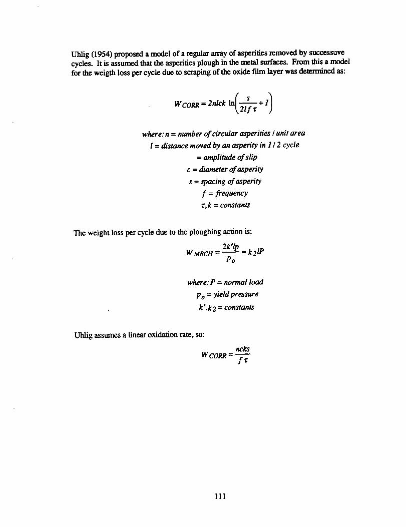
Uhlig (1954)proposed a model of a regulararrayof asperitiesremoved by suc.,cessuve
cycles. It is assumed that the asperities plough in the metal surfaces. From this a model
for the weigth loss per cycle due to scraping of the oxide fdm layer was determined as:
WCORR=2nlck in(2--:--fz+ 1)
where: n = number of circular asperities / unit area
l - distance moved by an asperity in 1 / 2 cycle
= amplitude of slip
c = diameter of asperity
s = spacing of asperity
f = frequency
z, k = constants
The weight loss per cycle due to the ploughing action is:
2 'lpW MECH = _ = k 21P
Po
where: P = normal load
Po = yield pressure
k', k 2 = constants
Uhlig assumes a linear oxidation rate, so:
ncksW CORR =
111
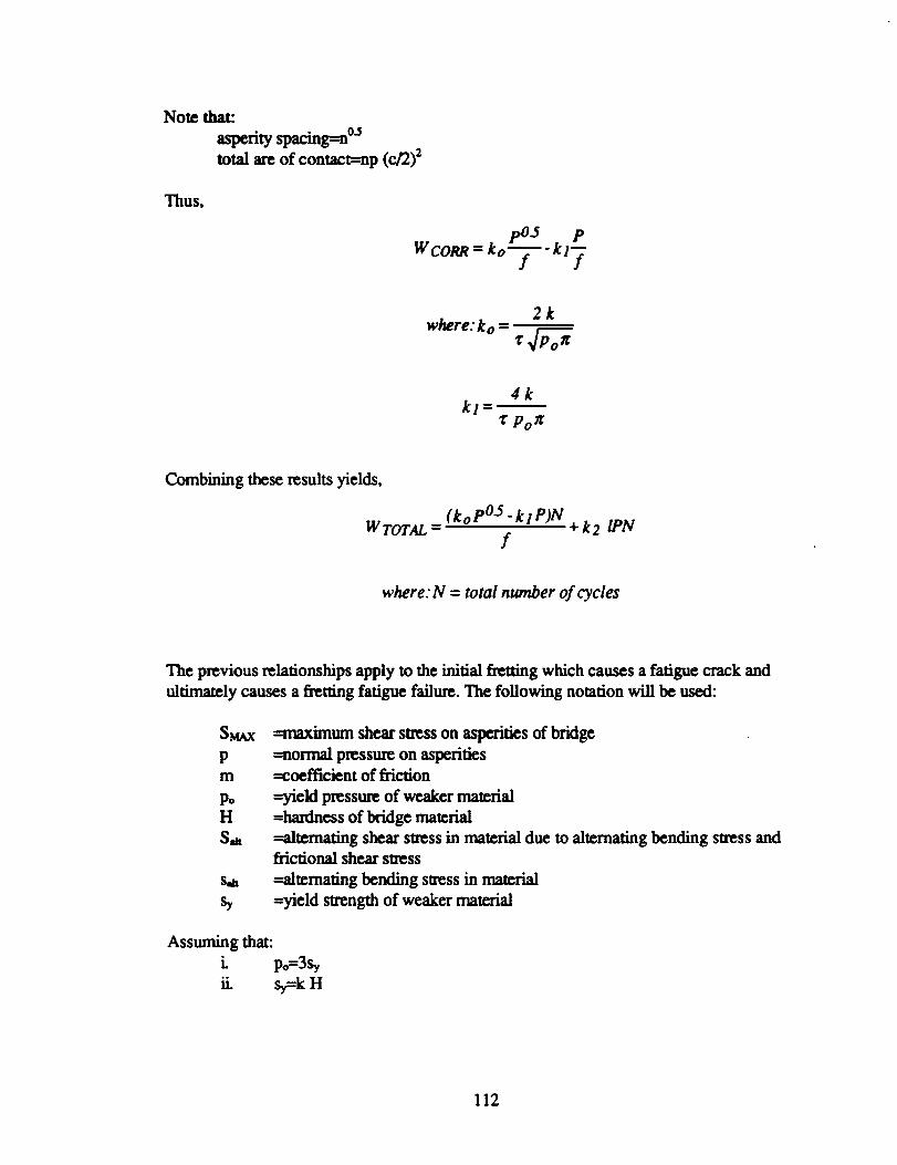
Note that:
asperity spacing=n °'_
total are of contact--rip (c/2) 2
Thus,
pO3
WCOP.R-ko--T-kl f
2kwhere: ko = r-'-
T ,Ip
4kkl =_
"¢po _
Combining these results yields,
(ko p03. kl P)NW TOTAL = + k 2 IPN
f
where: N = total number of cycles
The previous relationships apply to the initial fretting which causes a fatigue crack and
ultimately causes a fretting fatigue failure. The following notation will be used:
SMAX
Pm
PoH
S_
Salt
sy
--maximum shear stress on asperities of bridge
--normal pressure on asperities
=coefficient of friction
--_eld pressure of weaker material
=hardness of bridge material
_temating shear stress in material due to alternating bending stress andfrictional shear stress
---alternating bending stress in material
=yield strength of weaker material
Assuming that:
i. po=3Sy
ii. sr=k H
112
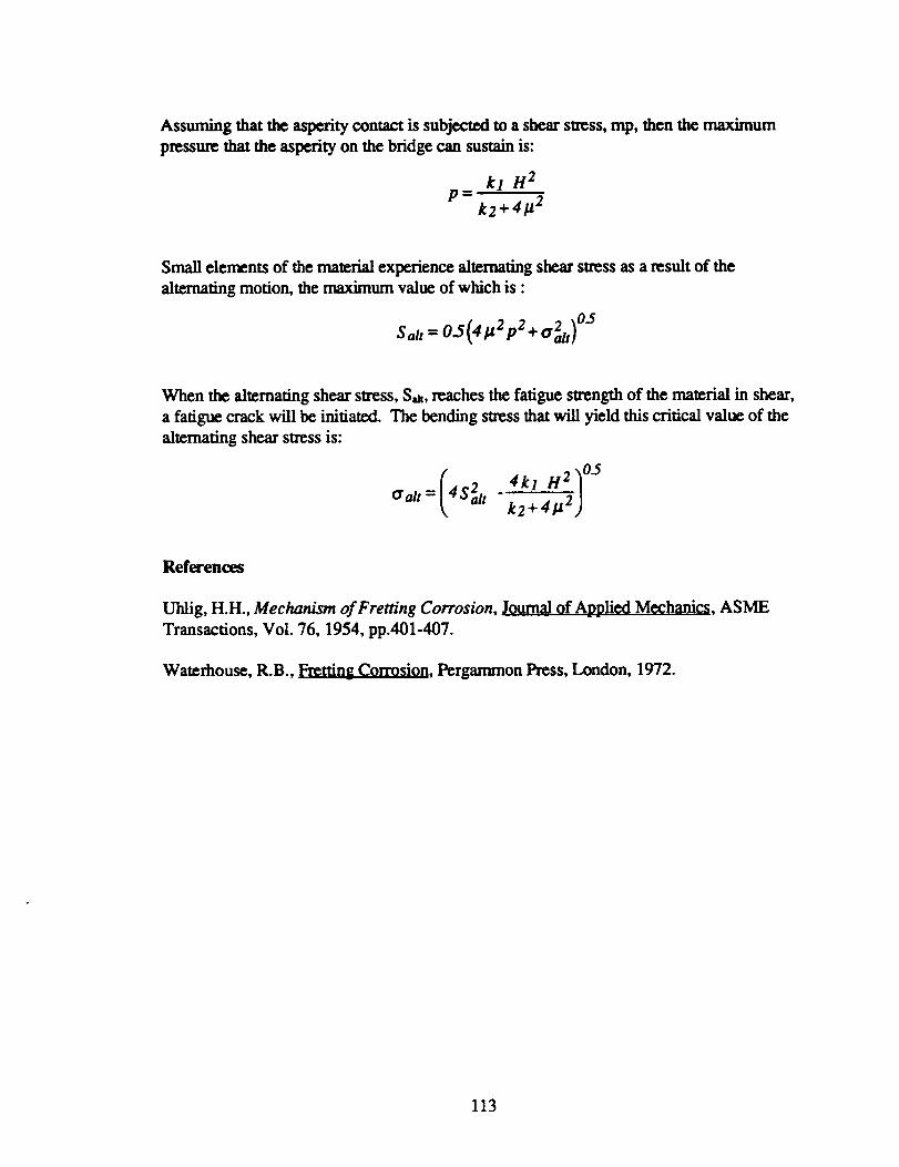
Assumingthat the asperity contact is subjected to a shear stress, mp, then the maximum
pressure that the asperity on the bridge can sustain is:
kl H 2p=
k2+4# 2
Small elements of the material experience alternating shear stress as a result of the
alternating motion, the maximum value of which is :
S alt = O.5(4122 p 2 + 02t) 05
When the alternating shear stress, S_t, reaches the fatigue strength of the material in shear,
a fatigue crack will be initiated. The bending saess that will yield this critical value of the
alternating shear stress is:
H2 _05trait = 4 S 21t 4 k lk2+4"-_)
References
Uhlig, H.H., Mechanism of Fretting Corrosion, Journal of Applied Mechanics, ASME
Transactions, Vol. 76, 1954, pp.401-407.
Waterhouse, R.B., Fretting Corrosion, Pergammon Press, London, 1972.
113
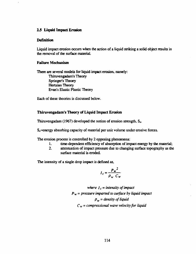
2.5 Liquid Impact Erosion
Definition
Liquid impact erosion occurs when the action of a liquid striking a solid object results in
the removal of the surface material.
Failure Mechanism
Thee are several models for liquid impact erosion, namely:
Thiruvengadam's Theory
SpringeesTheoryHertzian Theory
Evan's Elastic Plastic Theory
Each of these theories is discussed below.
Thiruvengadam's Theory of Liquid Impact Erosion
Thiruvengadam (1967) developed the notion of erosion strength, S¢.
So=energy absorbing capacity of material per unit volume under erosive forces.
The erosion process is controlled by 2 opposing phenomena:
1. time-dependent efficiency of absorption of impact energy by the material;
2. attenmation of impact pressure due to changing surface topography as thesurface material is eroded.
The intensity of a single drop impact is defined as,
pw 2[c =
Pw Cw
where I c = intensity of impact
Pw = pressure imparted to surface by liquid impact
P w = density of liquid
C w = compressional wave velocity for liquid
114
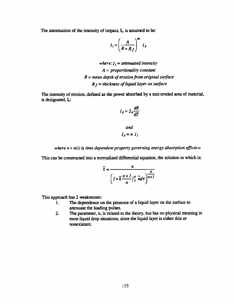
The auentuarion of the intensity of impact, I_, is assumed to be:
where: l i = attenuated intensity
A = proportionality constant
R = mean depth of erosion from original surface
R f = tlu'ckness of liquid layer on surface
The intensity of erosion, defined as the power absorbed by a unit eroded area of material,
is designated, I,:
dR
le = Se'_
and
le=n li
where n + n(t) is time dependent property governing energy absorption efficieiu
This can be constructed into a normalized differential equation, the solution to which is;
3= nn
This approach has 2 weaknesses:
1. The dependence on the presence of a liquid layer on the surface to
attenuate the loading pulses.
2. The paran_ter, n, is related to the theory, but has no physical meaning in
most liquid drop situations, since the liquid layer is either thin or
nonexistant.
!i5
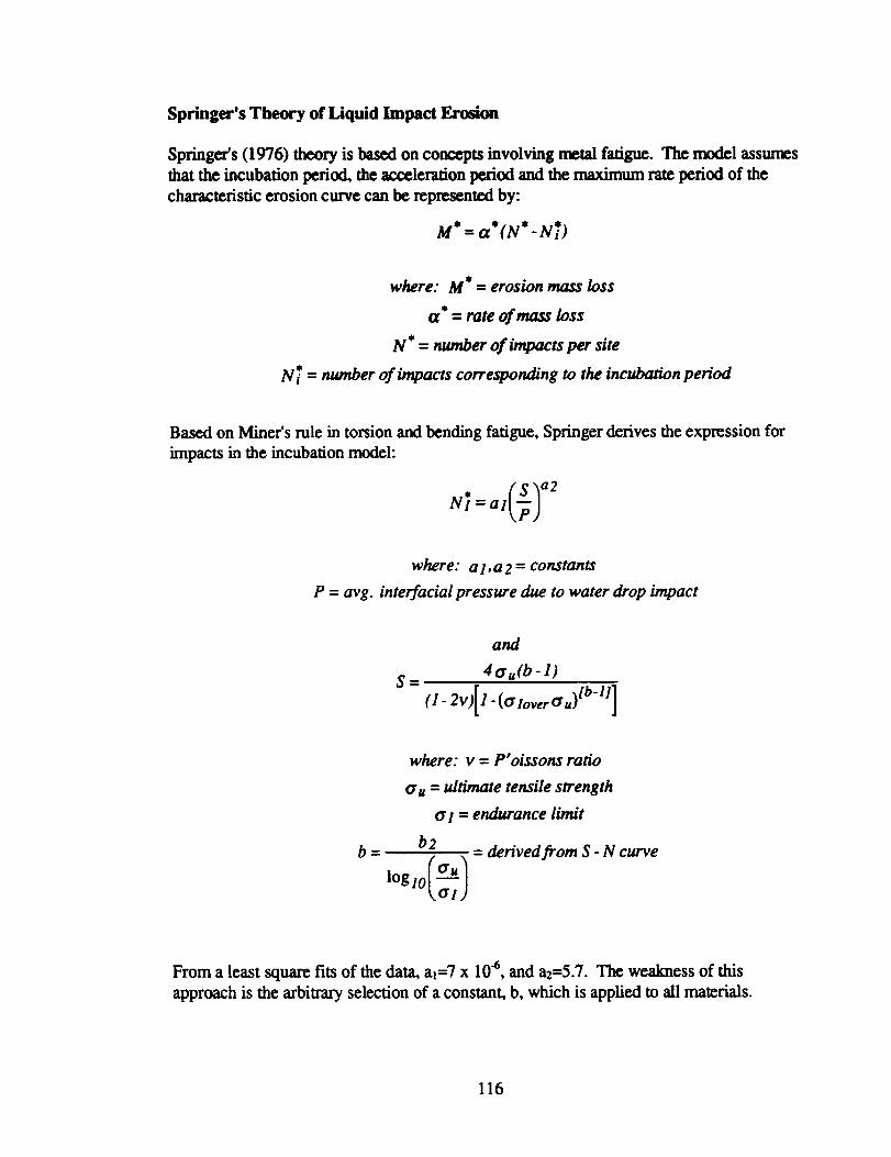
Springer's Theory of Liquid Impact Erosion
Springer's(1976) theoryisbased on concepts involvingmetal fatigue.The model assmnes
that the incubation period, the acceleration period and the maximum rate period of the
characteristic erosion curve can be represented by:
M• f a• (N•. N *)
where: M • = erosion mass loss
ot = rateof mass loss
N* = number of impacts per site
N_ = number of impacts corresponding to the incubation period
Based on Miner's rule in torsion and bending fatigue, Springer derives the expression for
impacts in the incubation model:
where: al,a2 = constants
P = avg. interfacial pressure due to water drop impact
S_
and
4au(b-1)
.m
where: v = P" oissons ratio
¢ru = ultimate tensile strength
¢71 = endurance limit
b2 = derived from S - N curve
From a least square fits of the data, a,=7 x 10 "6, and a2=5.7. The weakness of this
approach is the arbitrary selection of a constant, b, which is applied to all materials.
116
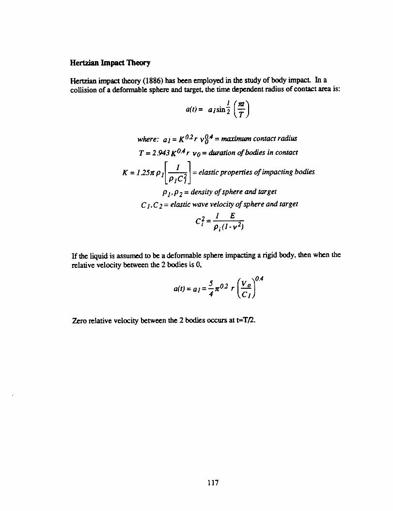
Hertzian Impact Theory
Hertzian impact theory (1886) has been employed in the study of body impact. In a
collision of a deformable sphere and target, the time dependent radius of contact area is:
a(t)= alsin-_
where: a l = K 0"2r V 0"4 -- maximum contact radius
T = 2.943 KO.4r vo = duration ofbodies in contact
K= 125_rPllp--_l=elasticpropern'es of impacting bodiest._.l
P l , P 2 = density of sphere and target
C1, C2 = elastic wave velocity of sphere and target
C2 = 1 EP i (I - V 2)
If the liquid is assumed to be a deformable sphere impacting a rigid body, then when the
relative velocity between the 2 bodies is O,
5_r02 r(Vo_ 0"4a(t) = a1= 7 _,-_1)
Zero relative velocity between the 2 bodies occurs at t=T/2.
117
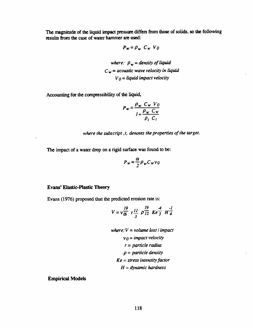
The rmgnimde of the liquid impact pressure differs from those of solids, so the following
results from the case of water hammer are used:
Pw =pw Cw VO
where: Pw = density of liquid
C w = acoustic wave velocity in liquid
V O = liquid impact velocity
Accounting for the compressibility of the liquid,
Pw Cw VOPw-
Pw Cw1+
Pt Ct
where the subscript ,t, denotes the properties of the target.
The impact of a water drop on a rigid surface was found to be:
Pw='_PwCwvO
Evans' Elastic-Plastic Theory
Evans (1976) proposed that the predicted erosion rate is:
19 19 -4 -1
V=v_- r 11 P-_ Ke 7 H_3
Empirical Models
where: V = volume lost / impact
v O= impact velocity
r = particle radius
,p = particle density
Ke = stress intensity factor
H = dynamic hardness
118
Due to the complex nature of the processes involved in impact erosion, the u'aditionai
approach has been the utilization of models fitted to empirical data. Schmitt (1970) has
proposed that impact erosion be modelled using equations of the form:
MDPR = KV a sin E 0
where: MDPR = mean depth of penetration rate
K ffi constant
V = velocity
8 = impact angle
a,]_ = empirically determined exponents
Schmitt notes that uncouated 2-dimensionally reinforced composite materials, beta of 2 is
a best fit for velocities between 450 and 1700 m/sec.
References
Evans, A.G., et al., Impact Damage in Brittle Material.¢ in the Plastic Response Re,me,
Contract No. 00014-75-C-0069, Report No. SC5023.9TR, Rockwell International Center,
Thousand Oaks, CA., 1976.
Hertz, H., Miscellaneous Pa_rs, Macmillan and Company, London, 1886.
Schmitt, G.F., Erosion Rate-Veloc#y Dependence for Materials at Supersonic Speeds,
CharacteriT_don and Determination of Erosion Resistance, ASTM-STP-474, American
Society for Testing and Materials, 1970.
Springer, G.S., Erosion by Liquid Impact, Scripta Publishing Co, J. Wiley, Washington,
D.C., 1976.
Thiruvengadam, A., The Concept of Erosion Strength, Erosion by Cavitation or
ASTM-STP-408, American Society for Testing and Materials, 1967.
119
3._
Corrosion is the destructive attack of a metal by cherr6cal or electrochemical reaction with
it environment (Uhlig, 1971). The destruction of a metal surface by physical causes is not
classified as corrosion.
The major classifications of corrosion given by Fontana (1986) are:
.
2.
3.
4.
5.
6.
7.
8.
9.
Erosion-corrosion
Galvanic corrosion
Uniform attack
Pitting corrosionCavitation
Crevice corrosion
Stress corrosion cracking
Selective leaching
Intergranular corrosion
Models for the first six forms of corrosion were found, and are presented in sub-sections 1
through 6 that follow. At this time no deterministic relationships were found that
accurately predict stress corrosion cracking, selective leaching, or intergranular corrosion.
References
Fontana, M., Corrosion Engineering, 3rd Edition, McGraw-Hill Book Co., San Francisco,
1986.
Uhlig, H., Corrosion and Corrosion Control, 2nd Edition, I. Wiley & Sons, New York,
1971.
120
3.1 Erosion-Corrosion
Definition
Erosion-corrosionis definedastheacceleratedcorrosionof a metal as a result of a
flowing fluid disrupting or thinning a protective film of corrosion products.
Failure Mechanism
The transition from laminar to turbulent flow occurs over a velocity range and is
dependent on the geometry, surface roughness, and liquid viscosity. The conditions of
fluid flow and the wansition to turbulent flow is predicted using the Reynolds number:
VdRe =_
Y
where:V = velocity( m / s)
d = characteristic specimen length (m)
y = kinematic viscosity (m 21 s)
When a liquid exhibits predominantly turbulent flow, a thin laminar sublayer, of thickness
dh, exists near the metal surface as a result of viscous drag. If material is being removed
from the metal surface there will be a diffusional boundary layer of thickness &l, (Poulson,
1983). The Schmidt number describes the relationship between these two boundary
layer5"
D
where: D = diffusivity of the relevant species (m / s)
As the value of the Schmidt number increases the diffusion layer will become thinner, and
its formation occur more rapidly (Poulson, 1983).
In most cases the resistance of the surface to mass transfer, both laminar and turbulent
regions of flow, is accomplished through the definition of the mass transfer coefficient, K,
as:
--.
rate of reaction
concentration driving force
121
Themasstransferrateis moreconvenientlydescribedby adimensionlessnumber,theSherwoodnumber,
KdSh =
D
For reactions that are governed by mass lransfer, the relationship between the Sherwood,
Reynolds, and the Schmidt numbers is found by empirical results to be of the form,
Sh = constant * Re x * Sc Y
Typical experimental results indicate that x is usually 0.3-1, and y is 0.33. These values
are applicable in cases where the surface is initially smooth. The case of rough surfaces
subjected to mass transfer is outlined below. In addition, the consideration of different
surface configurations that may be subject to erosion-corrosion is accommodated by the
constant in the above equation, a constant that is geometry dependent. The most
cormnon geometries studied, and some results are outlined in the next section.
When a metal is subjected to erosion corrosion it will develop scallop shaped ridges. The
roughening due to the creation of these ridges tends to increase the mass transfer rate, and
the rateof erosioncorrosion.The availabilityofrelationshipsdef'mingeithermass transfer
orerosioncorrosionfrom rough surfacesisextremelylimited.Recent work has indicated
thatonce a surfaceisroughened, the roteof mass transferisgoverned by roughness, not
the geometry of the surface(Poulson,1990). More importantly,the resultsindicatethata
universalgoverning relationshipformass transferforroughened surfacesmay exist,
namely,
Sh = 0.01 Re Sc 033
The results indicating such a result axe shown in Figure 1, taken from Poulson (Corr. Sc.,
1990). Poulson does indicate that the main differences between geometries is their
tendency to roughen; he cites that bends in pipes tend to roughen faster, probably as a
result of their attaining a critical Reynolds number more easily. Although the smooth
surfacemass transferrelationshipsareusefulforthe predictionof initialratesoferosion
corrosion,the roughened surfacerelationshipwillgovern theerosioncorrosionprocess
once the surfaceisno longersmooth. The precisepointatwhich theroughened surface
relationshipisapplicablehas yet tobe established.
122
References
Abdulsalam, M., and J.T. Stanley, Steady-State Model for Erosion-Corrosion of
Feedwater Piping, Corrosion, Vol. 48, no. 7, pp. 587-593, 1992.
Heitz, E., Chemo-Mechanical Effects of Flow on Corrosion, Corrosion Eng_ineering, Vol.
47, no. 2, pp. 135-145, 1991.
Kappesser, R., I. Comet, and R. Greif, Mass Transfer to a Rough Rotating Cylinder,
ElectrQchemical Science, Dec. 1971, pp. 1957-1959.
Markin, A.N., I.S. Sivokin, and A.G. Krushodov, Mathematical Simulation of Corrosion-
Electrochemical Processes, Corrosion, Vol. 47, no. 9, pp. 659-664, 1991.
Nesic, S., and J. Postlethewaite, Relationship between the Structure of Disturbed Flow
and Erosion-Corrosion, Corrosion, Vol. 46, no. 11, pp. 874-880, 1990.
Nesic, S., and J. Postlethewaite, A Predictive Model for Localized Erosion-Corrosion,
Corrosion, Vol. 47, no. 8, pp. 582-589, 1991.
Nesic, S., and J. Postlethewaite, Hydordynamics of Disturbed Flow and Erosion-
Corrosion: Part 1-Single-Phase Flow Study, Canadian Journal of Chemical En_ncering,
Vol. 69, pp.698-710, June 1991.
Poulson, B., Electrochemical Measurements in Flowing Solutions, Corrosion Science,
Vol. 23, no. 4, pp. 391-430, 1983.
Poulson, B., Mass Transfer.from Rough Surfaces, Corrosion Science, Vol. 30, no. 6/'7,
pp. 743-746, 1990.
123
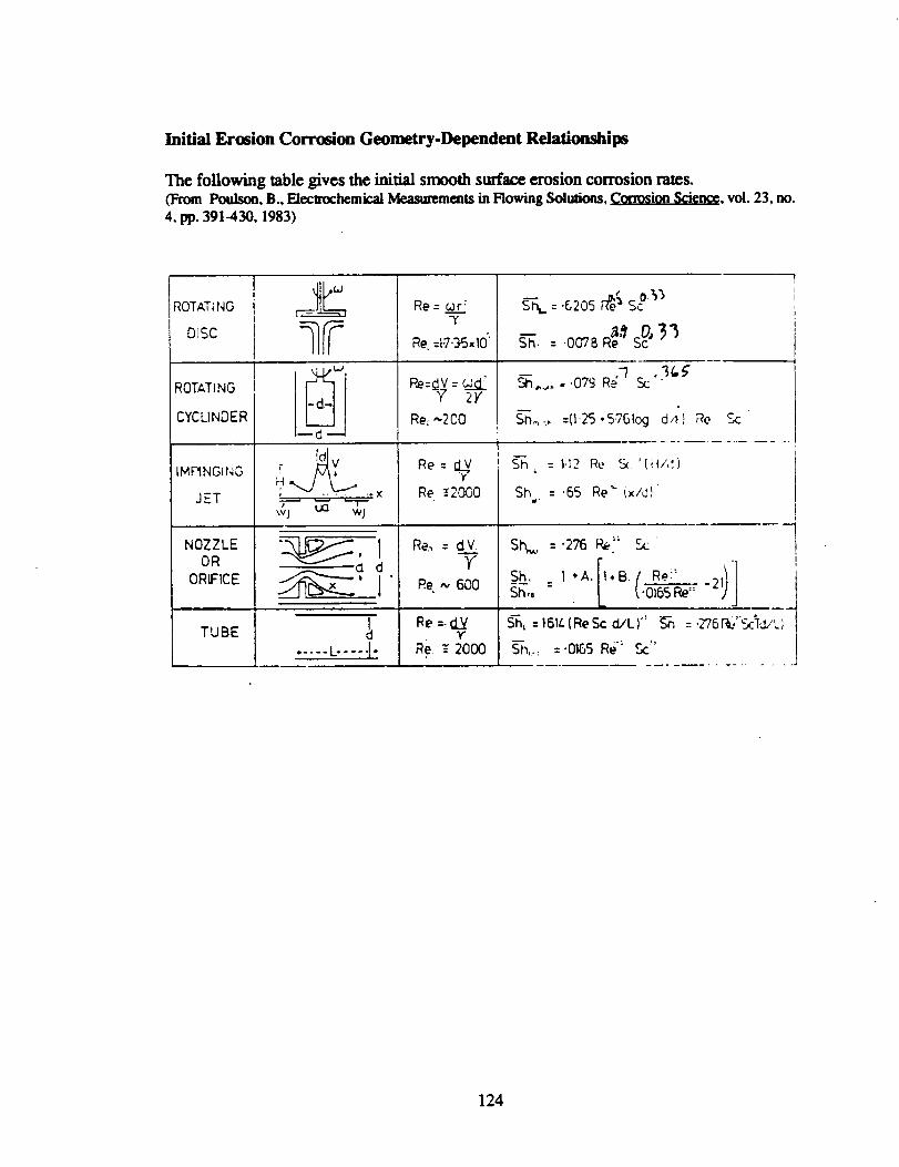
Initial Erosion Corrosion Geometry-Dependent Relationships
The following table gives the initial smooth surface erosion corrosion rates.(From Poulson, B., Eleclrochemicai Measurements in Rowing Solutions, Corrosion Science, vol. 23, no.
4, pp. 391-430, 1983)
;ROTATING
D}SC
ROTATING
CYCLINDER
IMPINGING
JET
NOZZLE
OR
ORIFICE
TUBE
"--t.-v_j ua wj
Re -- _r:h"
Re,=1-7-35xI0:
Re=_Re _2000
Re,_ = dV.
YRe. ,,, 6O0
_,,.,...079 R#-7s_ "t('_
s-g_:, =I_-25.576bg d,{)Re
Sh = 1.12Re Sc 'fill,i)
Sin = .65 Re _"(x/d)w'
Si'_, = '276 Re:: Sc
,)gh-',o: .0_'-_'; - 2i
Re =._y-
i% :-2000
S-h, =t61LlReSc d/L)" _ =-2"/6_,"_14,/LJ
SI--_.... = "0165 Re_ Sc_'
124
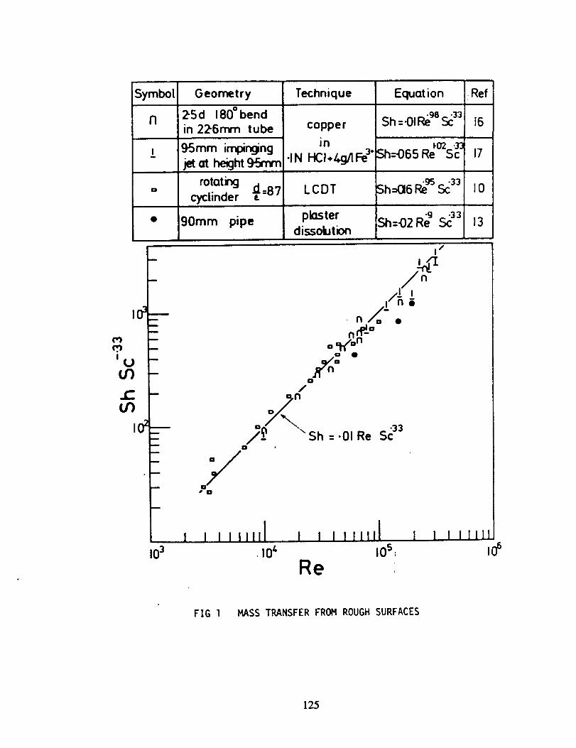
Symbol
n
I
O
Geometry
2-5d 180° bendin 22"6rWTI tube
95mm impinging
jet at height 9=Jr_n,
rotating d=87cyclinder t
Technique
copper
in
•IN HCI.,.Z,_JIFe3°
LCDT
Equot ion .Ref
Sh=431Re98Sc33 16
sh_-06sR;°_S_,7
Sh=O6Re9sSc33
90ram pipe plasterdissolution
sh=o2R_,_sc_
10
13
io_
qlI
UU')
JEul
io;
n
m
I
m
m
D
m
m
m
103
/I
LI a
n/_=- ,,
o •
fO
_ "Sh=.OIRe Sc330
0
0JO
I0 _" 10si
Re
FIG l MASS TRANSFER FROM ROUGH SURFACES
125
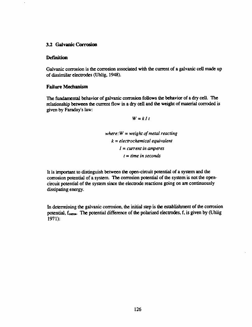
3.2 Galvanic Corrosion
Definition
Galvanic corrosionisthe corrosionassociatedwith thecurrentof a galvaniccellmade up
of dissimilarelectrodes(Uhlig,1948).
Failure Mechanism
The fundamental behaviorof galvaniccorrosionfollowsthebehaviorof a dry ceil.The
relationship between the current flow in a dry cell and the weight of material corroded is
given by Faraday's law:
W=klt
where: W = weight of metal reacting
k = electrochemical equivalent
I = current in amperes
t = time in seconds
k is important to distinguish between the open-circuit potential of a system and the
corrosion potential of a system. The corrosion potential of the system is not the open-
circuit potential of the system since the electrode reactions going on are continuously
dissipating energy.
In determining the galvanic corrosion, the initial step is the establishment of the corrosion
potential, f,_. The potential difference of the polarized electrodes, f, is given by (Uhlig
1971):
126
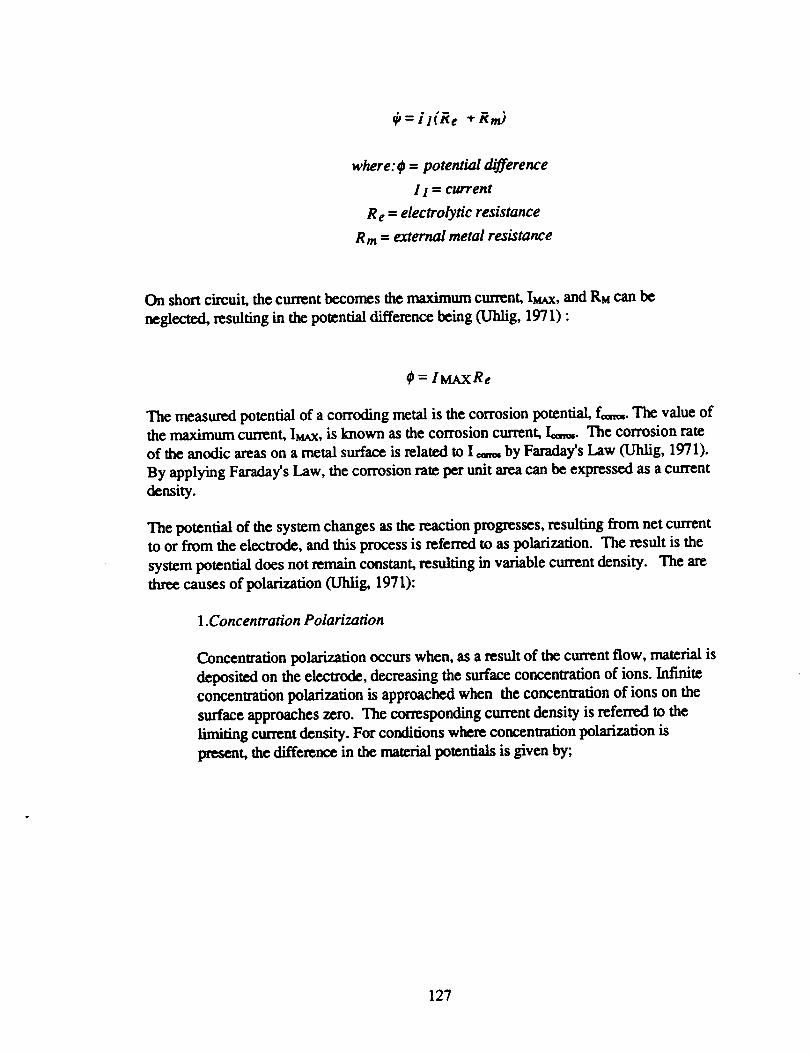
- il(Re * Rr_
where: _ = potential difference
I 1 = current
Re = electrolytic resistance
Rm = external metal resistance
On short circuit, the current becomes the maximum current, IMAX, and RM call be
neglected, resulting in the potential difference being (Uhlig, 1971) :
??= I MAX R e
The measured potential of a corroding metal is the corrosion potential, f¢,_.. The value of
the maximum current, I_x, is known as the corrosion current, I,_o.. The corrosion rate
of the anodic areas on a metal surface is related to I _ by Faraday's Law (Uhlig, 1971).
By applying Faraday's Law, the corrosion rate per unit area can be expressed as a current
density.
The potential of the system changes as the reaction progresses, resulting from net current
to or from the electrode, and this process is referred to as polarization. The result is the
system potential does not remain constant, resulting in variable current density. The are
three causes of polarization CtJldig, 1971):
1.Concentration Polarization
Concentration polarization occurs when, as a result of the current flow, material is
deposited on the electrode, decreasing the surface concentration of ions. Infinite
concentration polarization is approached when the concentration of ions on the
surface approaches zero. The corresponding current density is referred to the
limiting current density. For conditions where concentration polarization is
present, the difference in the material potentials is given by;
127
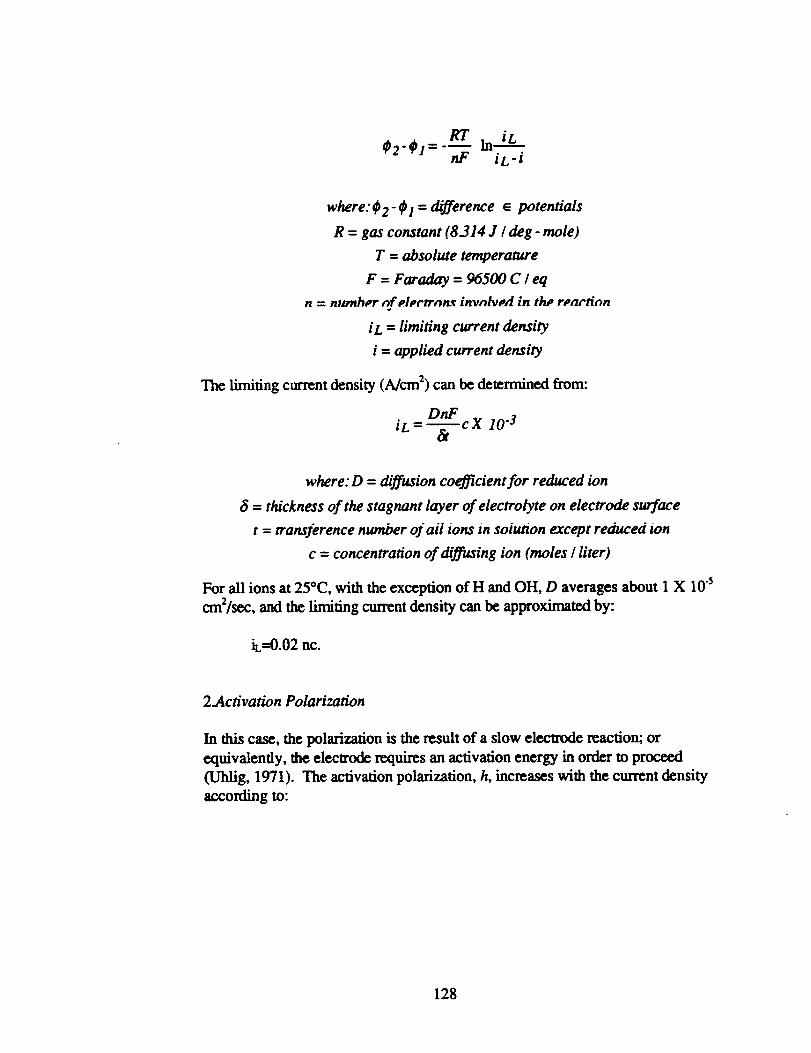
RT In i...A._L¢12" ¢_1= "-_ i L - i
where: ¢ 2-¢ l = difference _ potentials
R = gas constant (8314 J / deg - mole)
T = absolute temperature
F = Faraday = 96500 C I eq
n = manher of electrnn_ invalw,d in the reaction
i L = limiting current density
i = applied current density
The limiting current density (A/cm 2) can be determined from:
DnFiL = _c X 10 -3
&
where: D = _'ff'usion coefficient for reduced ion
5 = thickness of the stagnant layer of electrolyte on electrode surface
t = transference number ofaii ions tn soiunon except reduced ion
c = concentration of&'ffusing ion (moles / liter)
For all ions at 25"C, with the exception of H and OH, D averages about 1 X 10 "s
crn2/sec, and the limiting current density can be approximated by:
iL=0.02 nc.
2.Acn'vation Polarization
In this case, the polarization is the result of a slow electrode reaction; or
equivalently, the electrode requires an activation energy in order to proceed
(Uhlig, 1971). The activation polarization, h, increases with the current density
according to:
128
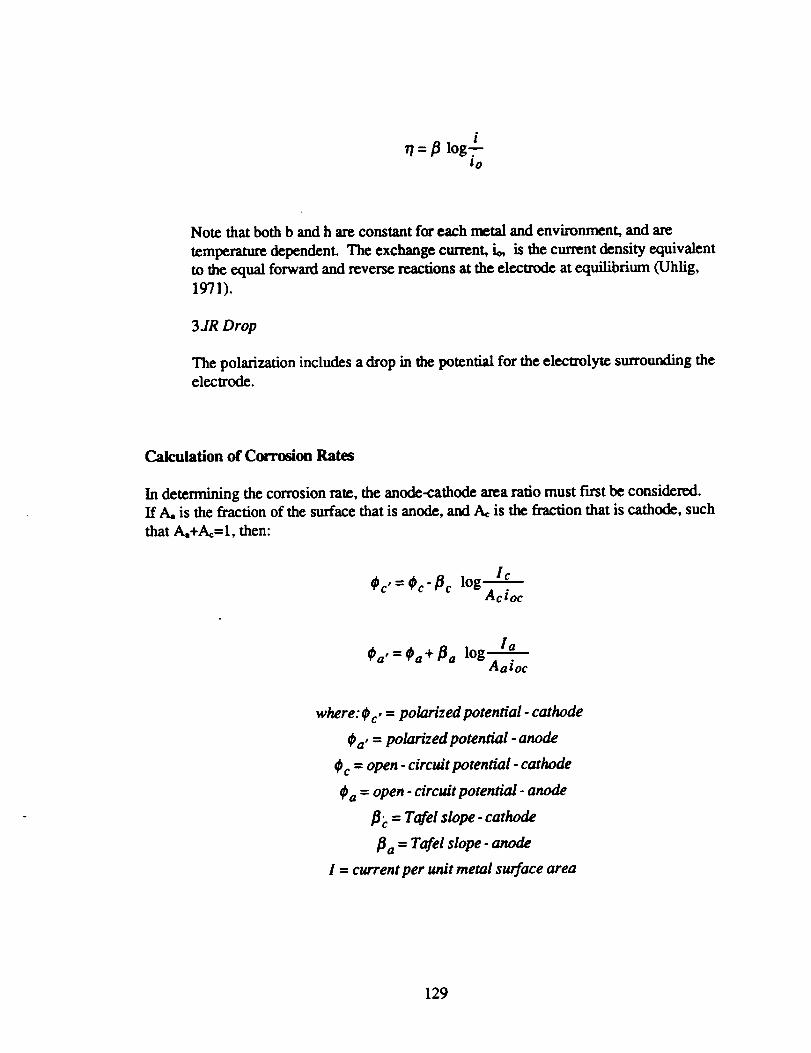
77= _ log _-_-lo
Note that both b and h axe constant for each metal and environment, and are
temperature dependent. The exchange current, io, is the current density equivalent
to the equal forward and reverse reactions at the electrode at equilibrium COhlig,
1971).
31R Drop
The polarization includes a drop in the potential for the elecu_lyte surrounding the
electrode.
Calculation of Corrosion Rates
In determining the corrosion rate. the anode-cathode area ratio must first be considered.
If A, is the fraction of the surface that is anode, and A_ is the fraction that is cathode, such
that A.+A_=I. then:
¢c,=#pc-Oc log IcAcioc
0a' =0a +_a log laAaioc
where: ¢ c, = polarized potential - cathode
Oa' = polarized potential - anode
¢ c = open - circuit potential - cathode
¢ a = open - circuit potential - anode
_'c = Tafel slope - cathode
_ a = Tafel slope - anode
I = current per unit metal surface area
129
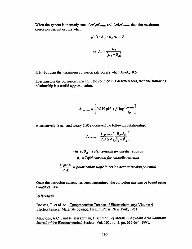
When the system is in steady state, fc---f°=£_,,., and I.=L-I_, then the maximum
corrosion current occurs when:
_c(l "Ac)"_cAc = 0
Oc
orAc- +/Ja)
If b_-=b,, then the maximum corrosion rate occurs when Ac=A_==0.5.
In estimating the corrosion cun'cnt, if the solution is a dearatexl acid, then the following
relationship is a useful approximation:
¢corros =-[O.O59 pH + fl log_]_o .1
Alternatively, Stem and Geary (1958), derived the following relationship:
I corros 23A tJ- -L)
A¢
where: fla = Tafel constant for anodic reach'on
_c = Tafel constant for cathodic reaction
= polarization slope in region near corrosion potential
Once the corrosion current has been determined, the corrosion rate can be found using
Faraday's Law.
References
Bockris, J., et al. ed., Comprehensive Treatise of Electrochemistry: Vloume 4
Electrochemical Materials Science, Plenum Press, New York, 1981.
Makrides, A.C., and N. Hackerman, Dissolution of Metals in Aqueous Acid Solutions,
Journal of the Electrochemical Society, Vol. 105, no. 3, pp. 612-634, 1991.
130

Stem,M., and A. Geary, Journal of the Electrochemical Society_, Vol. 104, No. 56, 1958.
Uhlig, H., The Corrosion Handbook, J. Wiley & Sons, New York, 1948.
Uhfig, H., Corrosion and Corrosion Control, Second Edition, J. Wiley & Sons, New
York, 1971.
131
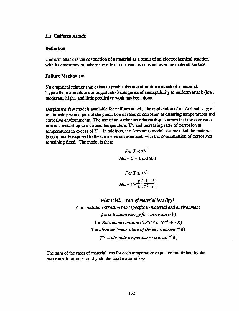
3.3 Uniform Attack
Definition
Uniform attack is the destruction of a material as a result of an electrochemical reaction
with its environment, where the rate of corrosion is constant over the material surface.
Failure Mechanism
No empirical relationship exists to predict the rate of uniform attack of a material.
Typically, materials are arranged into 3 categories of susceptibility to uniform attack (low,
moderate, high), and little predictive work has been done.
Despite the few models available for uniform attack, _e application of an Arrhenius type
relationship would permit the prediction of rates of corrosion at differing temperatures and
corrosive environments. The use of an Arrhenius relationship assumes that the corrosion
rate is constant up to a critical temperature, Tc, and increasing rates of corrosion at
temperatures in excess of Tc. In addition, the An'henius model assumes that the material
is con_ually exposed to the corrosive environment, with the concentration of corrosives
remaining fixed. The model is then:
For T < T C
ML = C = Constant
For T < T C
1 1
where: ML = rate of material loss (ipy)
C = constant corrosion rate: specific to material and environment
¢ = activation energy for corrosion (eV)
k = Boltzmann constant (0.8617x lO'4eV I K)
T = absolute temperature of the environment (°K)
T ¢ = absolute temperature - critical (o K)
The sum of the rates of material loss for each temperature exposure multiplied by the
exposure duration should yieldthetotalmaterialloss.
132
References
Uhlig,H.,The Corrosion Handbook, J.Wiley & Sons, New York, 1948.
Cruse ct al., Space Tran._portation System Life Management System Development. Phase
2, SwRI Project No. 06-2924, Report No. 06-2924-1A, Southwest Research Institute,
San Antonio, TX, 1989.
Cruse et al., STS Life M_a_ement System Development. SwRI Project No. 06-2148,
Report No. 06-2148-1A, Southwest Research Institute, San Antonio, TX, 1988.
133
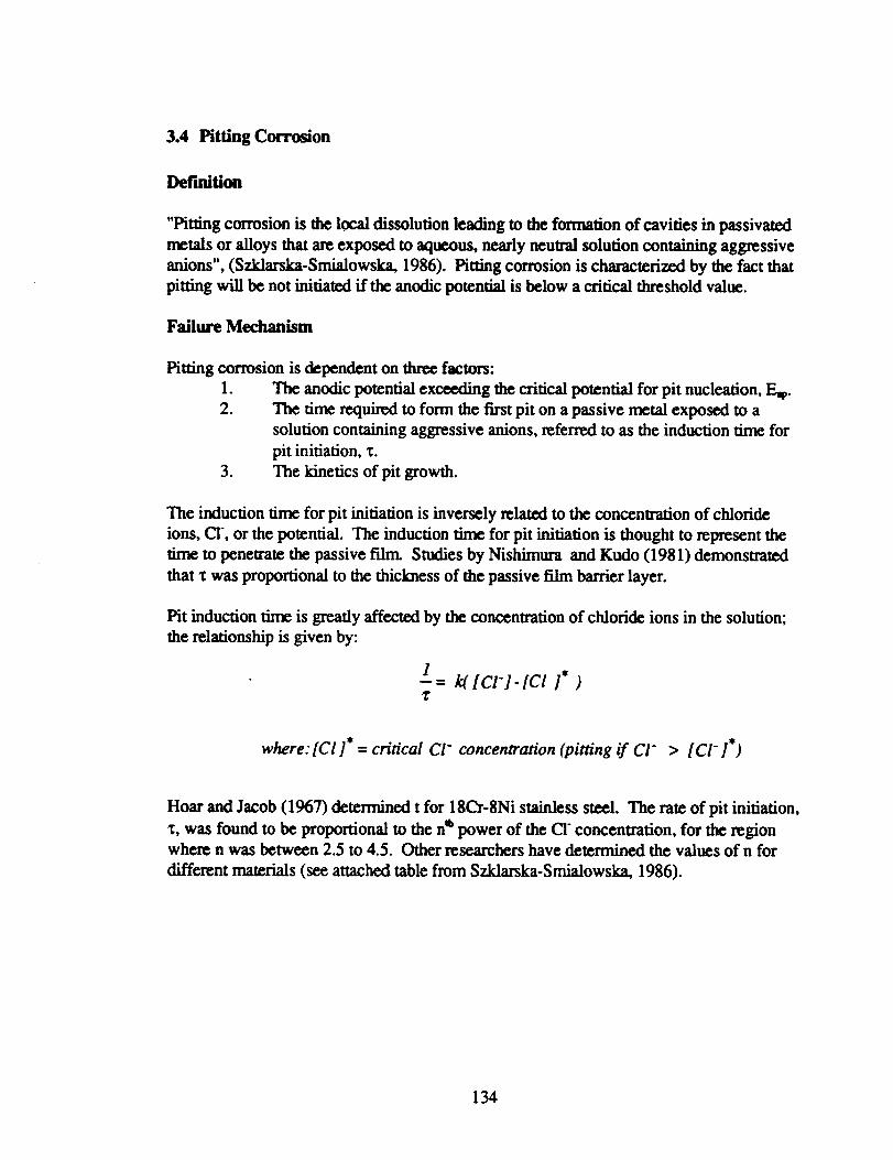
3.4 Pitting Corrosion
Definition
"Pitting corrosion is the local dissolution leading to the formation of cavities in passivated
metals or alloys that are exposed to aqueous, nearly neutral solution containing aggressive
anions", (Szklarska-Smialowska, 1986). Pitting corrosion is characterized by the fact that
pitting will be not initiated if the anodic potential is below a critical threshold value.
Failure Mechanism
Pitting corrosion is dependent on three factors:
1. The anodic potential exceeding the critical potential for pit nucleation, F__.
2. The time required to form the first pit on a passive metal exposed to a
solution containing aggressive anions, referred to as the induction time for
pit initiation, _.
3. The kinetics of pit growth.
The induction time for pit initiation is inversely related to the concentration of chloride
ions, CI', or the potential. The induction time for pit initiation is thought to represent the
time to penetrate the passive film. Studies by Nishimura and Kudo (1981) demonstrated
that x was proportional to the thickness of the passive film barrier layer.
Pit induction time is greatly affected by the concentration of chloride ions in the solution;
the relationship is given by:
1__= [CI']- [el l* )T
where: [Cl ]* = critical Cl" concentration (pitting if CI" > [Cl" ]* )
Hoar and Jacob (1967) determined t for 18Cr-8Ni stainless steel. The rate of pit initiation,
_, was found to be proportional to the n" power of the CI" concentration, for the region
where n was between 2.5 to 4.5. Other researchers have determined the values of n for
different materials (see attached table from Szklarska-Smialowska, 1986).
134
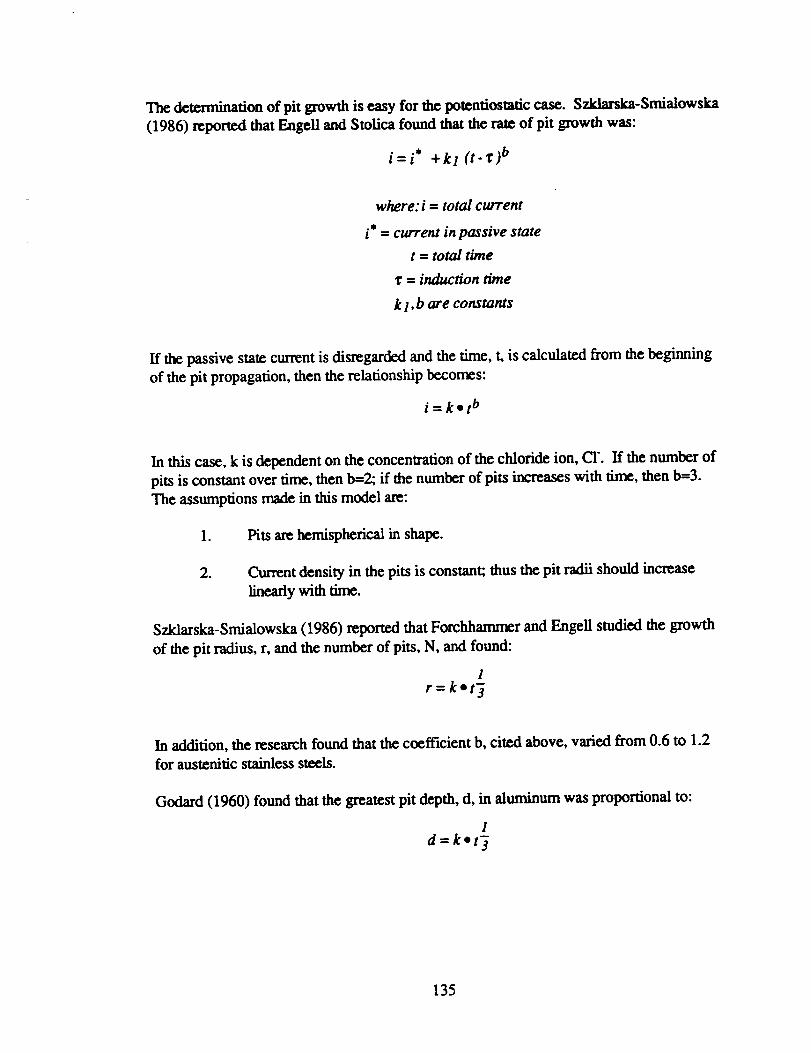
The determination of pit growth is easy for the potentiostatic case. Szklarska-Smialowska
(1986) reported that Eager and Stolica found that the rate of pit growth was:
i=t +kl (t'g) b
l
where: i = total current
= current in passive state
t = total time
x = induction time
k 1 ,b are constants
If the passive state current is disregarded and the time, t, is calculated from the beginning
of the pit propagation, then the relationship becomes:
i=ketb
In this case, k is dependent on the concentration of the chloride ion, el. If the number of
pits is constant over time, then b=2; if the number of pits increases with time, then b=3.
The assumptions made in this model are:
1. Pits are hemispherical in shape.
. Current density in the pits is constant; thus the pit radii should increase
linearly with time.
Szklarska-Smialowska (1986) reported that Forchhammer and Engell studied the growth
of the pit radius, r, and the number of pits, N, and found:
1r=kot_
In addition, the research found that the coefficient b, cited above, varied from 0.6 to 1.2
for austenitic stainless steels.
Godard (1960) found that the greatest pit depth, d, in aluminum was proportional to:
I
d=k't'_
135
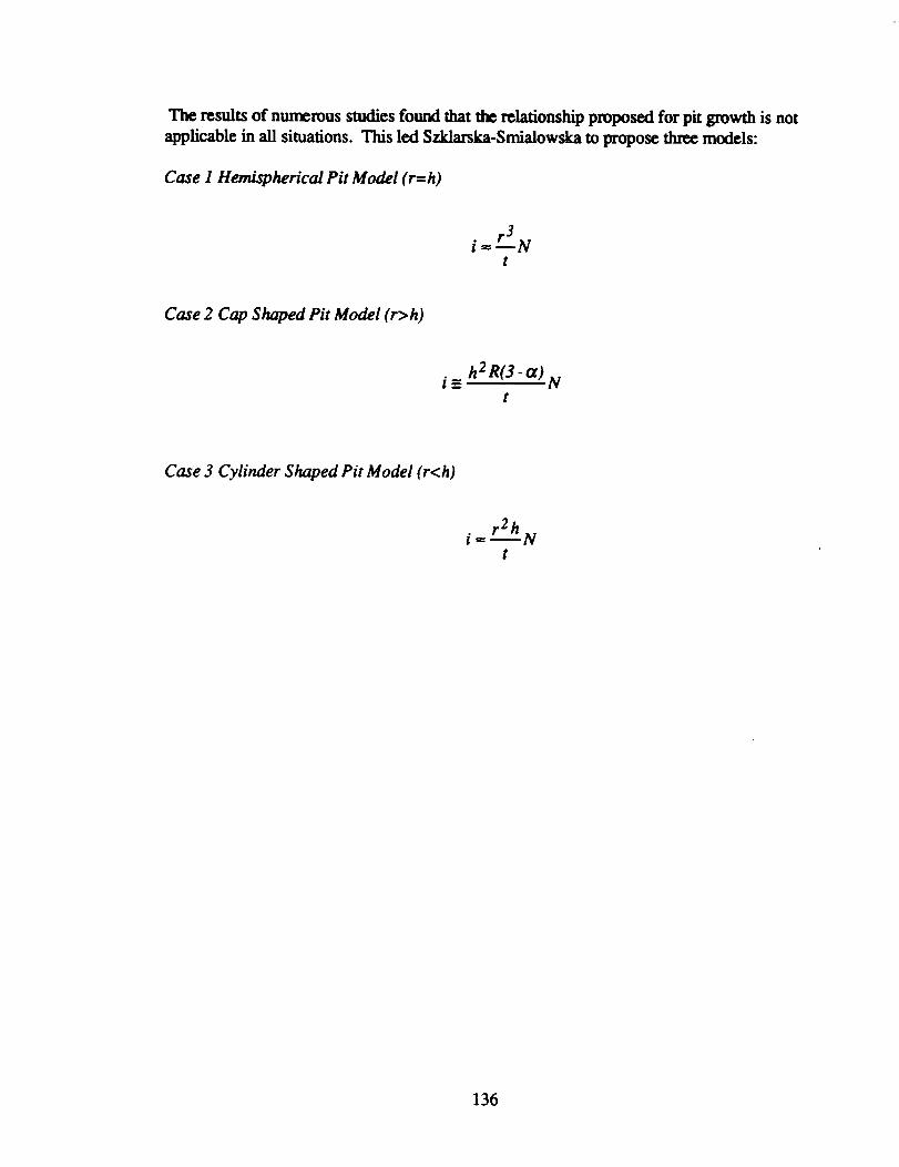
The results of nurr_rous studies found that the relationship proposed for pit growth is not
applicable in all situations. This led Szldarska-Smialowska to propose three models:
Case I Hemispherical Pit Model (r=h)
i= r3Nt
Case 2 Cap Shaped Pit Model (r>h)
i =_ h2 R(3a) N
Case 3 Cylinder Shaped Pit Model (r<h)
i=r2hNt
136
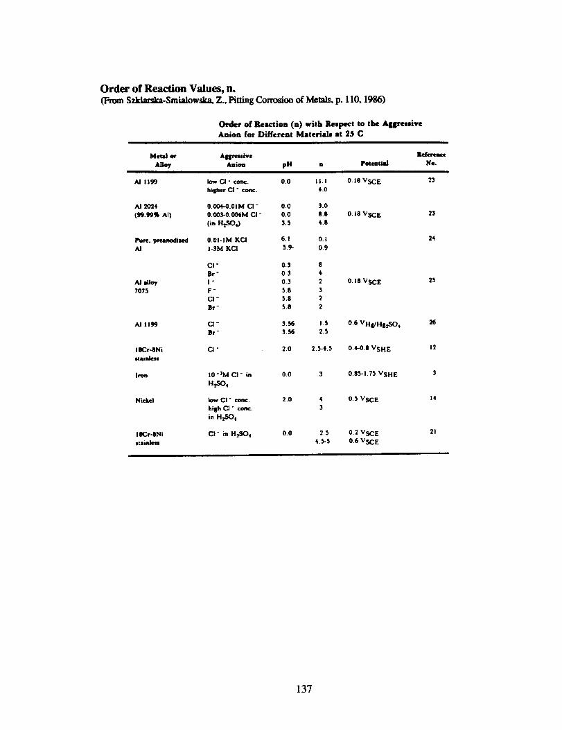
Order of Reaction Values, n.(From Szklarska-Smialowska, Z., Pitting Corrosion of Metals, p. 110, 1986)
Order of Reaction (n) with Reepect to the Aggre_iveAnion for Different Materials st 25 C
Metal or AIIIv_ive
Alloy Amiom pH n Pmmtiai
Al 1199 low Ci- cone. 0.0 li.I 0.18 VSC E
hisher CI - conc. 4.0
AI 2024 O.O04-O.OIM CI- 0.0 3.0
(99.99% AI) 0.003-0.004M CI - 0.0 8.8 O. 18 VSC E
(in H_C),) 3.5 4.8
Pure, pceanodised 0.01-1M KCI 6.1 0.1AI I-3M KCI 5.9- 0.9
CI - 0.3 8
Br- 03 4
AI alloy I " 0.3 2 O. 18 VSC E
7075 F " $,8 3
CI - 5.8 2
Br - 5.8 2
AI 1199 CI ° 3.56 I.$ 0.6 VH|/H82SO 0
Br" 3.56 2.5
IBCr-SNi CI " 2.0 2.5-4+5 [email protected] VSH E
.miak._
Iron 10 "3M CI" in 0.0 3 0185-1.75 VSH E
ti_3,
Nickel low CI" ¢on¢. 2.0 4 0.5 VSC E
high CI" come. 3
in H_._O,
18Cr-SNi Ci" in Hp_O, 0.0 2.5 0.2 VSC E
stainJess 4.5-5 0.6 V_CE
23
23
24
25
26
12
3
14
21
137
Refexenees
Godard, H.P., Pitting Kinetics, Canl_lian Journal of Chemical Engineering, Vol. 38, p.
167, 1960.
Nishimura, R., and K. Kudo, Effect of Thickness and Composition of Films on the
Breakdown of Passivity oflron, Proceedings of the 8th Intemalional Congress on Metal
Corrosion, Mainz, DECHEMA, Frankfurt am Main, Vol. 1, p.6, 1981.
Szklarska-Smialowska, Z., pitting Corrosion of Metals, NACE, Houston, TX, 1986.
138
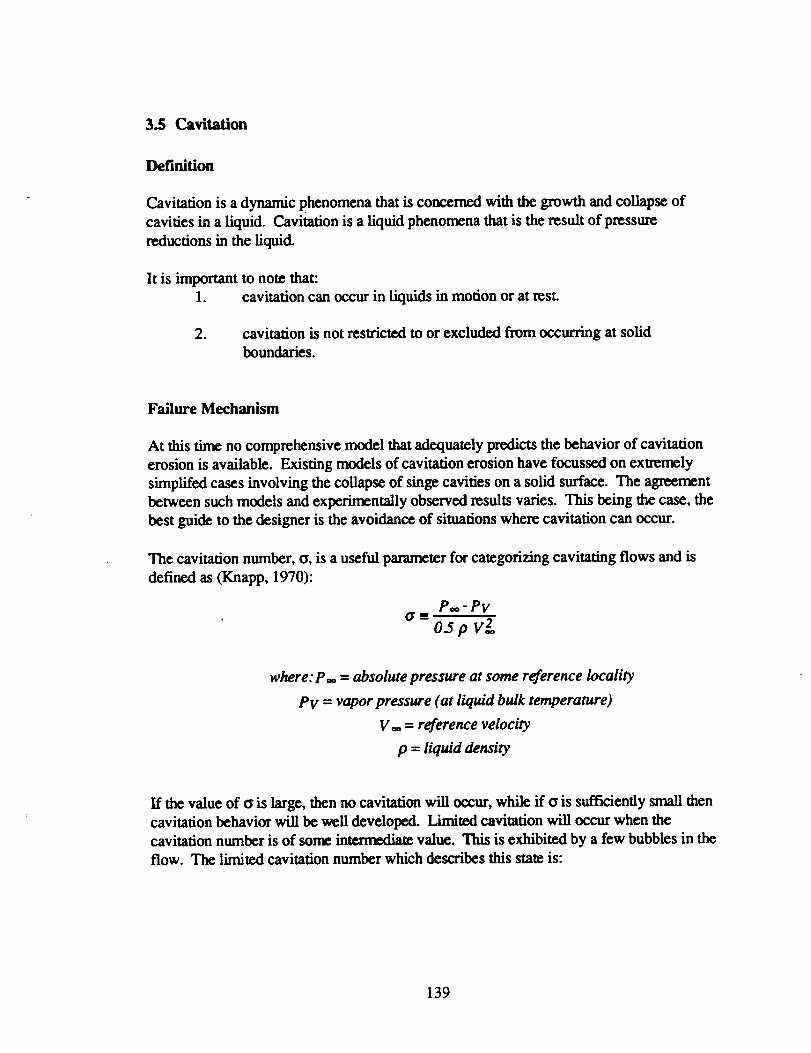
3.5 Cavitation
Definition
Cavitation is a dynamic phenomena that is concerned with the growth and collapse of
cavities in a liquid. Cavitation is a liquid phenomena that is the result of pressure
reductions in the liquid.
It is important to note that:
1. cavitation can occur in liquids in motion or at rest.
2. cavitation is not restricted to or excluded from occurring at solid
boundaries.
Failure Mechanism
At this time no comprehensive model that adequately predicts the behavior of cavitation
erosion is available. Exisling models of cavitation erosion have focussed on extremely
simplifed cases involving the collapse of singe cavities on a solid surface. The agreement
between such models and experimentally observed results varies. This being the case, the
best guide to the designer is the avoidance of situations where cavitation can occur.
The cavitation number, o, is a useful parameter for categorizing cavitating flows and is
defined as (Knapp, 1970):
Po. - PVCYm
o.5 p v 2.
where: P.o = absolute pressure at some reference locality
PV = vapor pressure (at liquid bulk temperature)
V.. = reference velocity
p = liquid density
If the value of o is large, then no cavitation will occur, wlKie if o is sufficiently small then
cavitation behavior will be well developed. Limited cavitation will occur when the
cavitation number is of some intermediate value. This is exhibited by a few bubbles in the
flow. The limited cavitation number which describes this state is:
139
P**L "PV¢yL =-
o.5p
Here, P..L is the absolute pressure at the reference locality that corresponds to the state of
limited cavitation.
The determination of the nature of cavitation has been studied with two different
approaches:
1.
.
Desinent Cavitation
In this case cavitation is established while holding the velocity constant,
and then increasing the pressure until the cavitation disappears at a
pressure value, referred to as the desinence pressure, P.o. The desinentcavitation number is determined from the same relation at that above, with
the exception that P. is replaced by P.o.
Incipient Cavitation
In this case velocity is held constant, eliminating all cavitation, and then the
pressure is decreased until cavitation appear at the inception pressure,P.._.
The incipient cavitation number is determinde by replacing P.. by P.._ and
applying the above relationships.
References
Holl, J.W., Limited Cavitation, Proceedings of the ASME Fluids Engineering and Applied
Mechanics Conference, Norhtwestern University, Evanston, IL, June 16-18, 1969.
Knapp, R.T., J.W. Daily, and F.D. Hammitt, Cavitation, McGraw-Hill Book Co., New
York, 1970.
140
3.6 Crevice Corrosion
Definition
"Crevice corrosion occurs when two or more surfaces in close proximity lead to the
creation of a locally occluded region where enhanced dissolution can occur", (SharlantL
1992). The rate of crevice corrosion is usually a function of the depth and width of the
crevice. The distinction between crevice corrosion and pitting is that crevice corrosion
proceeds at a much faster rate than pitting. This more rapid corrosion rate is a result of
the restrictive crevice geometry which permits the crevice electrolytic solution to under
change much more rapidly than a pit.
Failure Mechanism
The complex nature of crevice corrosion has made prediction of crevice corrosion rates
difficult. At present, no accurate deterministic model of crevice corrosion exits. The
current approach favored for the evaluation of crevice corrosion is the application of finite
element methods. A number of packaged computer programs are available to predict
crevice corrosion based on finite element methods, including:
CHEQMATE-CHemical EQuih'brium with Migration And Transport Equations
developed by A. Haworth, S.M. Sharland, P.W. Tasker, and C.J. Tweed outlined
in Harwell Laboratory Report, NSS-R113, 1988.
HARWELL-presented by C.P. Jackson, The TSGL Finite-Element Subroutine
Library, AERE Report AERE-R10713, 1982.
141
Governing Equations
'The transportation of aqueous species i is governed by the mass-balance equation. The
mass-balance equation describes the diffusion under concentration gradients,
electromigration under potential gradients, and chemical reaction', (Sharland, 1989). The
mass-balance equation is:
_C....._=Di A 2 Ci + zi UiFA(CiAcP) + Ri&
where: C i = concentration of species i
D i = effective diffusion coefficient
z i = charge number
Ri = rate of production / depletion of species i by chemical reaction
U i = mobility = D_..i.iRT
For a crevice geometry that is assumed to be rectangular, the steady-state transport
equations for species i is:
(_2Ci+_2Ci_+zi DiF [_x(Ci _O)+ _ (el _)]+Ri= 0
The boundary conditions are usually then determined.
References
Sharland, $.M., and P.W. Tasker, A Mathematical Model of Crevice and Pitting
Corrosion-1. The Physical Model, Corrosion Science, Vol. 28, no. 6, pp. 603-620, 1988.
$harland, S.M., and P.W. Tasker, A Mathematical Model of Crevice and Pim'ng
Corrosion-I. The Mathematical Solution, Corrosion Science, Vol. 28, no. 6, pp. 621-630,
1988.
$harland, $.M., C.P. Jackson, and A.J. Diver, A Finite-Element Model of the Propagation
of Corrosion Crevices and Pits, Corrosion Science, Vol. 29, no. 9, pp. 1149-1166, 1989.
Sharland, S.M., A Mathematical Model of the Initiation of Crevice Corrosion in Metals,
Corrosion Science, Vol. 33, no. 2, pp. 183-201, 1992.
142
Walton,J.C.,Mathematical Modeling of Mass Transport and Chemical Reaction in
Crevice and Pim'ng Corrosion, Corrosion Science, Vol. 30, no. 8/9, pp. 915-928, 1990.
Watson, M.K., and J. Postlethewait¢, Numerical Simulation of Crevice Corrosion: The
Effect of the Crevice Gap Profile, Corrosion Science, Vol. 32, no. 11, pp. 1253-1262,
1991.
Watson, M.K., and J. Posflethewalte, Numerical Simulation of Crevice Corrosion of
Stainless Steel and Nickel Alloys in Chloride Solutions, Corrosion Science, Vol. 46, no.
7, pp. 522-530, 1990.
143
4. Fatigue
Definition
Fatigue failure is a general term given to the sudden and catastrophic separation of a
machine part into two or more pieces as a result of the application of fluctuating loads or
deformations over a period of time.
The major forms of fatigue are:
1. High-cycle fatigue
2. Low-cycle fatigue
3. Crack growth
4. Surface fatigue
Of the various types of fatigue, high-cycle fatigue, low-cycle fatigue, and crack growth.
Physical Process of Fatigue
The fatigue process consists of three stages:
°
2.
3.
Crack initiation phase
Subcritical crack propagationFmal fracture
Of these stages, most designers are concerned with crack initiation and subcritical crack
propagation.
Probability models of fatigue life
Because many of the factors involved are random in nature, the appropriate development
of analysis and design methodologies should be probabilistic. Two distributions that have
been widely used in fatigue studies are the loguormal and Weibull distributions. Use of the
lognormal distribution has been based primarily on arguments of mathematical expediency.
However, it has been pointed out that the hazard function for the lognormal model
decreases for large values of N. This does not agree with our physical understanding of
progressive deterioration resulting from the fatigue process. Nevertheless, the loguormal
distribution often seems to provide a'"good fit" of cycles to failure data. The WeibuU
distribution is based on more physical convincing arguments. Moreover, the WeibuU
distribution is well-suited for certain procedures of statistical extrapolation to large
systems.
144
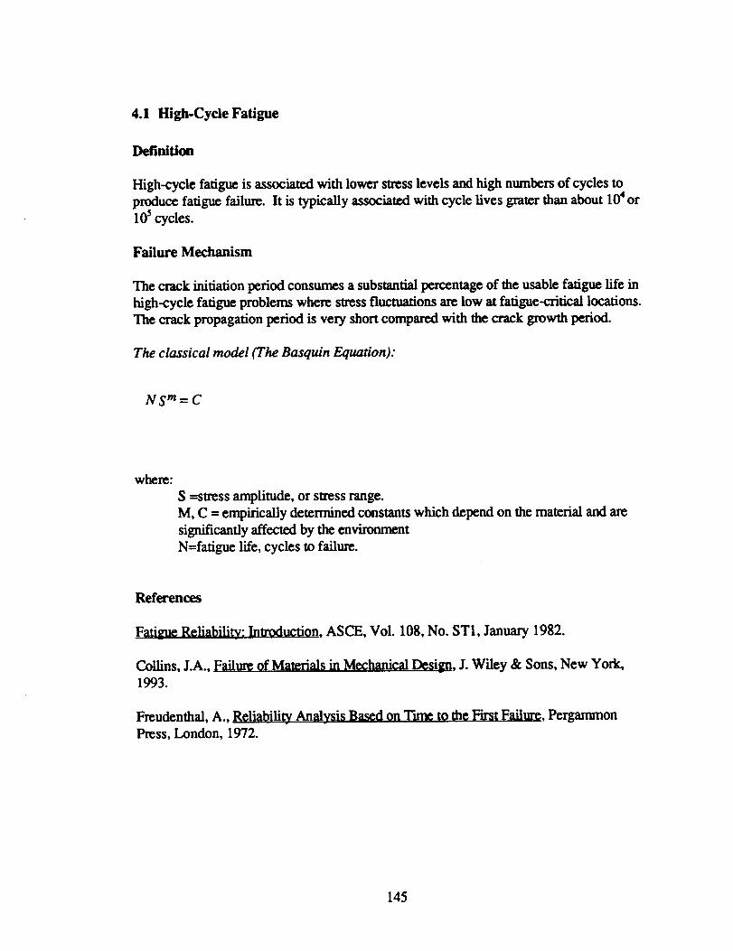
4.1 High-Cycle Fatigue
Definition
High-cycle fatigue is associated with lower stress levels and high numbers of cycles to
produce fatigue failure. It is typically associated with cycle lives grater than about 10 4 or
105 cycles.
Failure Mechanism
The crack initiation period consmr_s a substantial percentage of the usable fatigue life in
high-cycle fatigue problems where stress fluctuations are low at fatigue-critical locations.
The crack propagation period is very short compared with the crack growth period.
The classical model (The Basquin Equation):
NS m= C
where:
S =stress amplitude, or stress range.
M, C = empirically determined constants which depend on the material and are
significantly affected by the environment
N=fatigue life, cycles to failure.
References
F_tigue Reliability: Introduction, ASCE, Vol. 108, No. STI, January 1982.
Collins, J.A., Failure of Materials in Mechanical Desi__n, J. Wiley & Sons, New York,
1993.
Freudenthal, A., Reliabili _tyAnalysis Based on Time to the First Failure, Pergammon
Press, London, 1972.
145
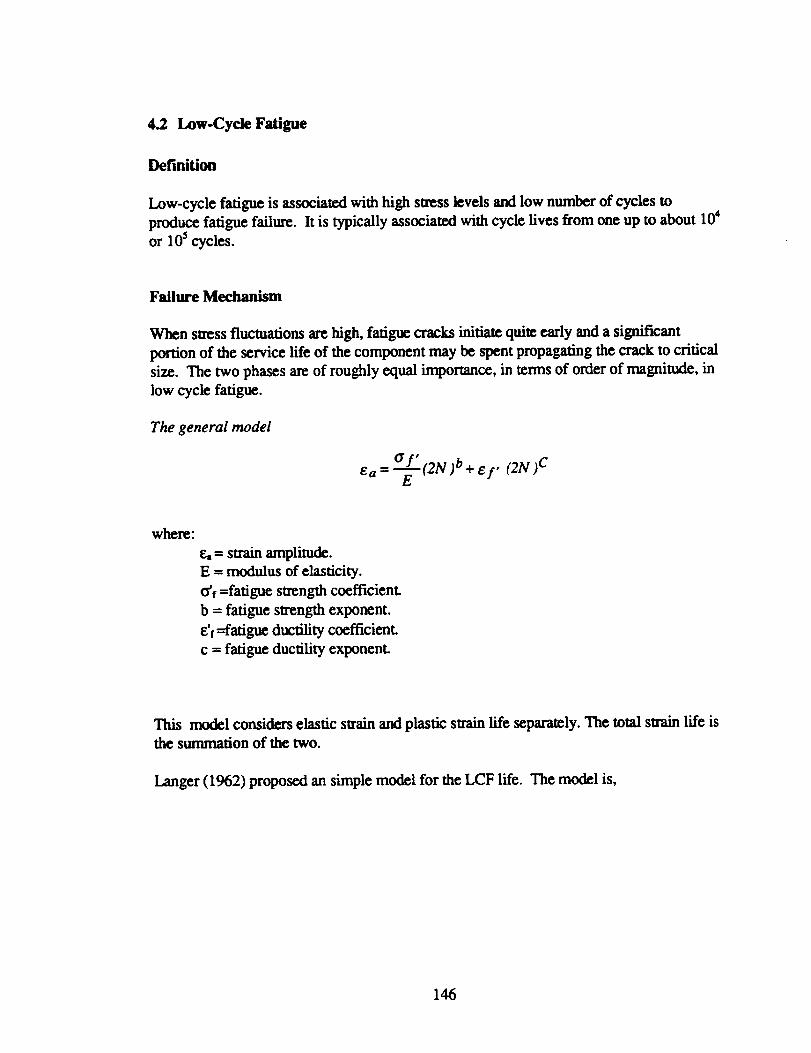
4.2 Low-Cycle Fatigue
Definition
Low-cycle fatigue is associated with high stress levels and low number of cycles to
produce fatigue failure. It is typically associated with cycle fives from one up to about 104
or 10 5 cycles.
Failure Mechanism
When stress fluctuations are high, fatigue cracks initiate quite early and a significant
portion of the service life of the component may be spent propagating the crack to critical
size. The two phases are of roughly equal importance, in terms of order of magnitude, in
low cycle fatigue.
The general model
ea = a-'_--_(2N )b+ Ef" (2N )C
where:
= strain amplitude.
E = modulus of elasticity.
¢¢f =fatigue strength coefficient.
b = fatigue strength exponent.
e'f-----'fatiguc ductility coefficient.
c = fatigue ductility exponent.
This model considers elastic swain and plastic slrain life separately. The total strain life is
the summation of the two.
Langer (1962) proposed an simple model for the LCF life. The model is,
146
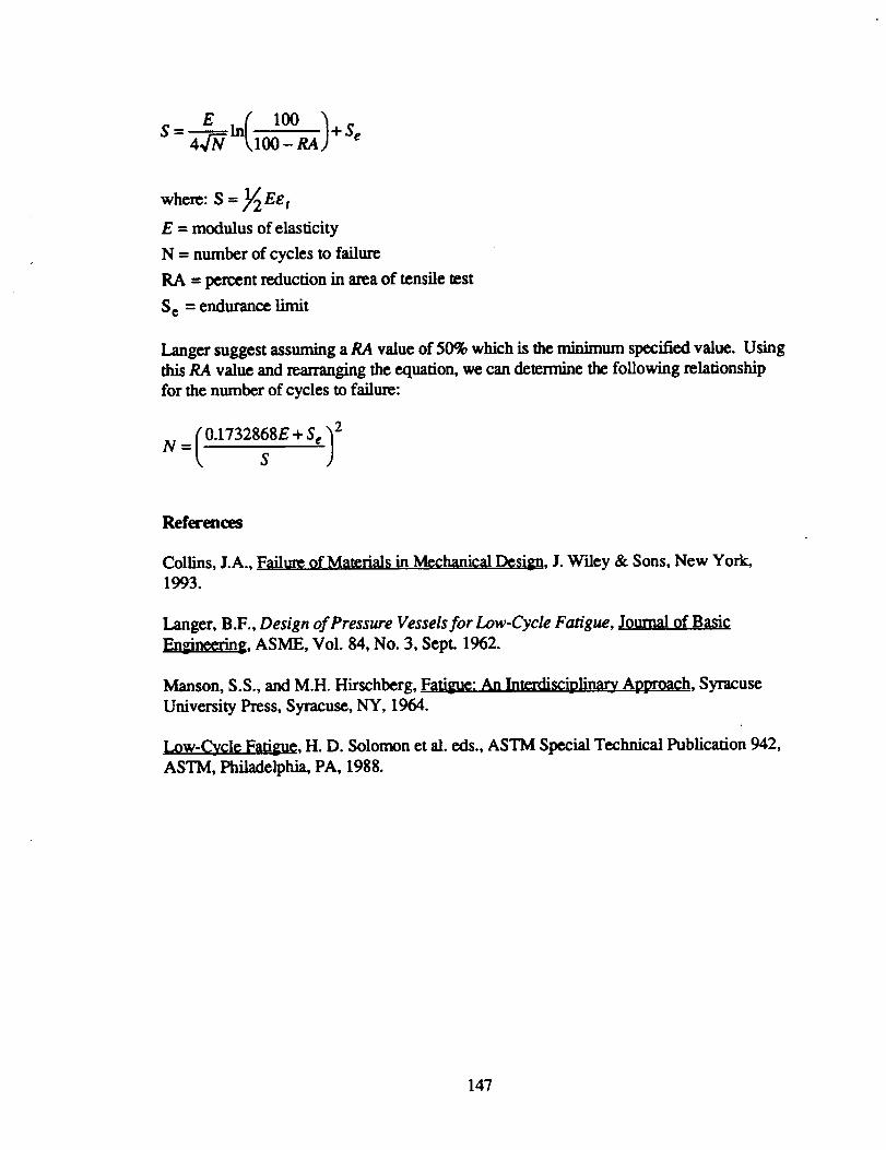
in(, loo ).s,s-- ,lOO-ea
where: S = _/2Eet
E = modulus of elasticity
N = number of cycles to failure
RA = percent reduction in area of tensile test
S e = endurance limit
Langer suggest assuming a RA value of 50% which is the minimum specified value. Using
this RA value and rearranging the equation, we can determine the following relationship
for the number of cycles to failure:
N =(O'17328_SE + Se ) 2
References
Collins, J.A., Failure of Materials in Mechanical Design, J. Wiley & Sons, New York,
1993.
Langer, B.F., Design of Pressure Vessels for Low-Cycle Fatigue, Journal of Basic
_, ASME, Vol. 84, No. 3, Sept. 1962.
Manson, S.S., and M.H. Hirschberg, Fatim_e: An Interdisciplinary_ Ap_m'oach, Syracuse
University Press, Syracuse, NY, 1964.
Low-Cycle Fatigue, H. D. Solomon et al. eds., ASTM Special Technical Publication 942,
ASTM, Philadelphia, PA, 1988.
147
4.3 Crack growth fatigue
Failure Mechanism
The crack growth rate is given by:
da= C(AK) n
dN
K = F(a)S.4_
where:
a = crack depth for a surface flaw or half-width for a penetration flaw.
F(a)= finite geometry correction factor which may depend on a.
K = stress intensity factor.
S = applied stress.
n, c =experimentally determined constants which depend on the mean cycling
streSS.
Reference
Collins, J.A., Failure of Materials in Mechanical Design, J. Wiley & Sons, New York,
1993.
148
5. Thermal Degradation
Definition
Thermal degradation is the deterioration of the functionality or physical properties of a
material due to the effects of temperature. The degradation is due solely to the effects of
temperature and does not involve other materials.
Failure Mechanism
The interest in thermal degradation lies in materials that are non-metallic, since thermal
influences on metals can result in changes in the grain structure. The material properties
of metals possessing different grain structures is well documented. As a result, this
examination of thermal degradation will focus primarily on polymers and insulating
materials.
In the case of polymers, the two main types of degradation are (Grassie, 1985) •
° Depolymerisation, which is the breaking of the main polymer chain
backbone so that at any intermediate stage the products are similar to the
parent material in that the monomer units remain distinguishable. The
products of the degradation may be monomer, or they may be volatile
chain fragments.
. Substitient reactions result in the attachment of substitients to the backbone
of the polymer molecules involved so that the chemical nature of the repeat
unit is changed even though the chain structure may remain intact.
In the case of polystyrene, if the chain scission occurs in a polymer molecule without
volatilisation, then (Grassie, 1985):
PoPt =_
(s+ l)
where: Po = initial chain length of the polymer
Pt = chain length of the polymer after time t
s = average number ofscissions per molecule
From this equation the fraction of broken bonds, _ can be found. If the chain scission is
random then e,=kt where k--rate constant for chain scission. If the chain contains weak
and strong links, then ¢x=_+kt, where _ is the fraction of weak links in the molecule.
149
In practice the approach is to determine the lifetime of polymers using approaches based
on An'henius equations. Bumay (1990) reports that a relationship that accounts for both
thermal and radiation degradation on polymers is:
where: E = activation energy
R = gas constant
T = absolute temperature polymer environment
T ref = reference temperature
k = radiation degradation reaction constant
D = dose rate
Note that E, k, and x are empirical constants. The parameter E can be determined from
the polymer where radiation is not a problem. Thus, k and x are empirically determined
from irradiation data. Burnay further reports that the majority of polymers studied have
been found to have x=l. For cases where x=l, the above relation is simply:
÷1a(T, D) = exp Tref " + k.D
This relationship is simply the sum of the thermal degradation described by the Arrhenius
relationship plus a dose rate component, D, multiplied by a radiation degradation reaction
constant, k. In cases where radiation is not significant, the relationship for simple thermal
degradation results.
Note that the parameter, a(T,D), is used as the constant deterioration rate in the Axrhenius
equation. By using the above relationships to determine the modified the deterioration
rate constant, the Arrhenius equation can consider the effects temperature and radiation on
polymer degradation.
References
Burnay, S.G., A Practical Model for Prediction of the Lifetime of Elastomeric Seals in
Nuclear Environments, Proceedings from 200th National Meeting of the American
Chemical Society, Washington, August 26-31, 1990 (Published in Radiation Effects on
Polymers. ACS Svm_tmsium Series #475)
150
Grassie, N., and G. Scott, Polymer Dcm'adation and Stabilization, Cambridge University
Press, Cambridge, U.K., 1985.
Schnabcl,W., Polymer Degradation,Macmillan PublishingCo.,New York, 1981.
Troitskii, B.B. and L.S. Troitskaya, Mathematical Models of the Initial Stage of the
Thermal Degradation of Poly (Vinyl Chloride), Journal of Polymer Science: Part A:
Polymer Chemistry, Vol. 28, pp. 2695-2709, 1990.
Proceedings from 200th National Meeting of the American Chemical Society,
Washington, August 26-31, 1990.
151
APPENDIXB
MECHANCIAL LIMIT STATES
USED
IN
FIRST-ORDER RELIABILITY MODELS
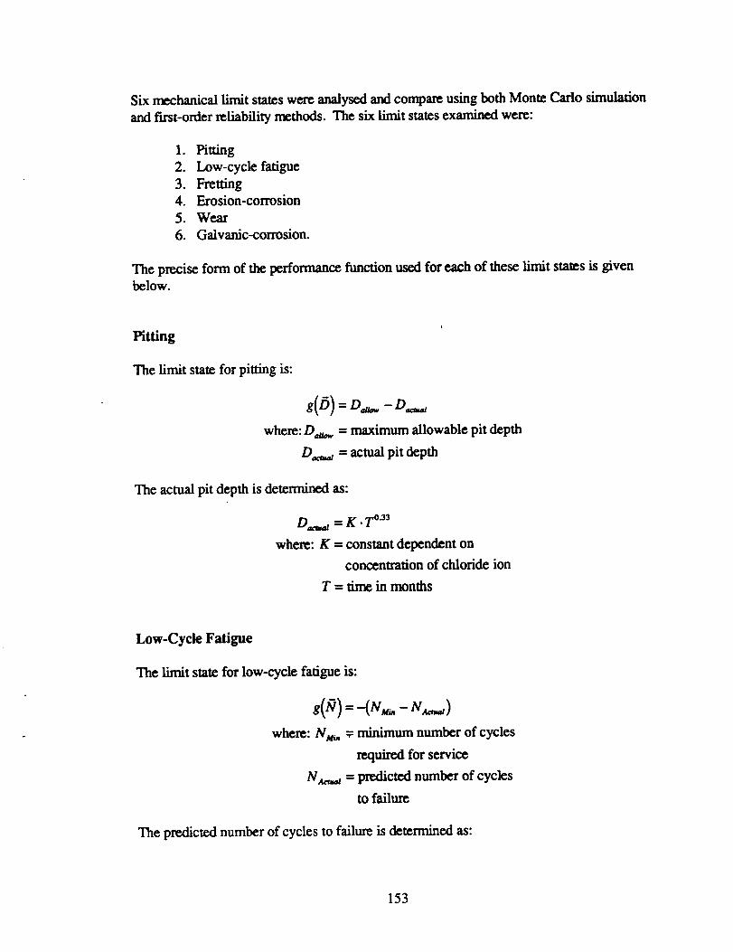
Six mechanical limit states were analysed and compare using both Monte Carlo simulation
and first-order reliability methods. The six limit states examined were:
1. Pitting
2. Low-cycle fatigue
3. Fretting
4. Erosion-corrosion
5. Wear
6. Galvanic-corrosion.
The precise form of the performance function used for each of these limit states is givenbelow.
Pitting
The limit state for pitting is:
where: D,_,. = maximum allowable pit depth
Dn,_ = actual pit depth
The actual pit depth is determined as:
D,_,,I = K. T °'33
where: K = constant dependent on
concentration of chloride ion
T = time in months
Low-Cycle Fatigue
The limit state for low-cycle fatigue is:
where: NM_, -_ minimum number of cycles
required for service
NA,,_ = predicted number of cycles
to failure
The predicted number of cycles to failure is determined as:
153
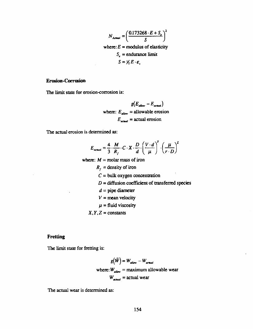
N,_,.,, a =(.0"17326_'E + S'.) 2
where: E = modulus of elasticity
S. = endurance limit
S = F2E.e.
Erosion-Corrosion
The limit state for erosion-corrosion is:
g(e.__- e._)where: E.,_ = allowable erosion
E,_,_ = actual erosion
The actual erosion is determined as:
° 1z=3 R_ 7_ " r-----_where: M = molar mass of iron
R/= density of iron
C = bulk oxygen concentration
D = diffusion coefficient of transferred species
d = pipe diamet.r
V = mean velocity
/a = fluid viscosity
X, Y, Z = constants
Fretting
The limit state for fretting is:
where: W,a_ = maximum allowable wear
W,_.,,a = actual wear
The actual wear is determined as:
154
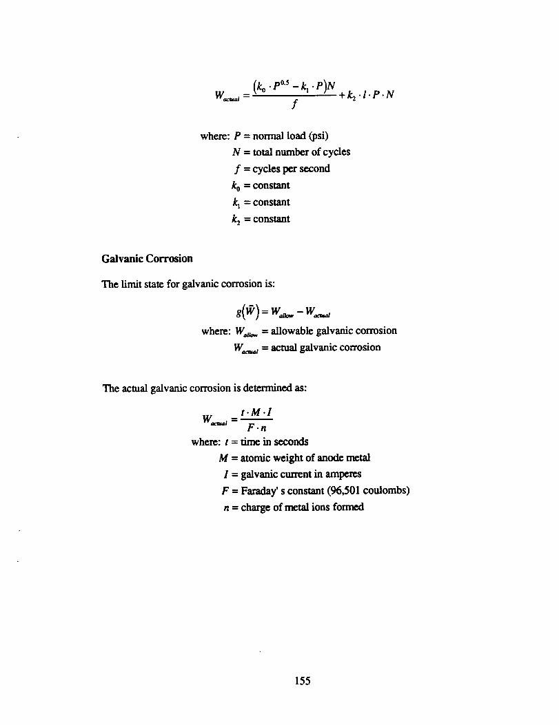
Wactua/ =(k0.,°°'5_ k_.p)/v
f
where: P
N
fk0
ks
= normal load (psi)
= total number of cycles
= cycles per second
= constant
= constant
= COP-stant
Galvanic Corrosion
The limit state for galvanic corrosion is:
where:
g( # ) = Wa_ - W_
W_ = allowable galvanic corrosion
W,_ = actual galvanic corrosion
The actual galvanic corrosion is determined as:
t.M.lW_=
F.n
where: t = time in seconds
M = atomic weight of anod¢ metal
I = galvanic current in amperes
F = Faraday' s constant (96,501 coulombs)
n = charge of rmtal ions formed
155
REFERENCES
1 Khmtchine, A. Ya., "Mathematisches uber die Erwartung yon einen offentlicher
SchaRer", MatemaRicbe Sborn_ 1932, quoted by R.E. Barlow and F. Proschan,
Mathematical Tbeo_ of Reliability_, J. Wiley and Sons, New York, 1965, p.1.
2 Palm, C., "Arbetskraftens Fordelning rid betjaning av automatskiner",
Indusuitidningen Norden, 1947, p.75, quoted by R.E. Barlow and F. Proschan,
Matl_matical Tbeo_ of Reliabili_, J. Wiley and Sons, New York, 1965, p.1.
3 Lotl_ A.L, "A Contribution to the Theory of Self-Renewing Aggregates with Special
Reference to Industrial Replacement", Annual of Mathematical Statistics, V. 10, 1939,
pp.1-25.
4 Campbell, N.R, "The Replacement of Perishable Members of a Continually Operating
System", Journal of the Royal Statistical Socie_, V. 7, 1941, pp. 110-130.
5 Feller, W., "On the Integral Equation of Renewal Theory", Annual of Mathematical
Statistics, V. 12, 1941, pp. 243-267.
6 Weibull, W., "A Statistical Theory of the Strength of Materials", Proceedings. Royal
Swedish Institute of Encneering Research, Stockholm, Sweden, No. 151, 1939.
7 Weibull, W,. "The Phenomenon of Rupture in Solids", Proceedings. Royal Swedish
Institute of En_neering Research, Stockholm, Sweden, No. 153, 1939.
8 Gumbel, E.J., "Les Valeurs Extremes des Distributions Statistiques", Annales de
l'Institute Henri Poincare, V. 4, Fasc. 2, 1935, p.115.
9 Rao, S.S., Reliabili_-Based Desi_, McGraw-Hill, New York, 1992, p. 15.
10 Rao, S.S., Reliabili_-Based Design, McGraw-Hill, New York, 1992, p. 15.
11 Rao, S.S., Reliabili_-Based Desi_, McGraw-HiU, New York, 1992, p.16.
12 Rao, S.S., Reliabili_-Based Desi_, McGraw-Hill, New York, 1992, p.16.
13 Rao, S.S., Reli_bili_-Based Desi_, McGraw-Hill, New York, 1992, p.16.
14 H_ndbook of ReliabilityPredictionProceduresforMechanical Equipment,
CARDEROCKDIV, NSWC-92/L0 I,Cardcrock Division,Naval SurfaceWarfare
Center,Bethesda, MD, 1992.
15 Madsen, H.O., S. Krenk, and N.C. Lind, Methods of Structm'al Safety, Prentice-Hall,
Englewood Cliffs, NJ, 1986, p. 2.
156
16 Madsen,H.O.,S. Krcnk, and N.C. Lind, Methods of Structural Safety, Prentice-Hall,
Englewood Cliffs, NJ, 1986, p. 3.
17 Cornell, C.A., "Bounds on the Reliability of Structural Systems", Journal of the
Structural Division, ASCE, V. 93, 1967, pp.171-200.
18 Lind, N.C., "The Design of Structural Design Norms", Journal of Stnmmral
Mechanics, V. 1, No. 3, 1973, pp. 35?-3?0.
19 Ditlevsen, O., "Structural Reliability and the Invariance Problem", Research Report
No. 22, Solid Mechanics Division, University of Waterloo, Waterloo, Canada, 1973.
20 Lind, N.C., "The Design of Structural Design Norms", Journal of Su'uctural
Mechanics, V. 1, No. 3, 1973, pp. 35?-3?0.
21 Hasofer, A.M., and N.C. Lind, "'Exact and Invariant Second Moment Code Format".
Journal of the Engineering Mechanics Division, ASCE, V. 100, 1974, pp. 111-121.
22 Rackwitz, R., and B. Fiessler, "Slxucmral Reliability Under Combined Random Load
Sequences", Computers and Structures, V. 9, 1978, pp. 489-494.
23 Diflevsen, O., "Narrow Reliability Bounds for Structural Systems", Journal of
Structural Mechanics, B. 7(4), 1979, pp. 453-472.
24 Cruse, T.C., Q. Huang, S. Mehta, and S. Mahadevan, "System Reliability and Risk
Assessment", Paper No. AIAA-92-2345, Proceedings of the 33rd Structures.
Structural Dynamics and Materials Conference, Dallas, Texas, 1992, pp. 424-432.
25 Boothroyd, G., and P. Dewhurst, Desi_m for Assembly, University of Massachusetts,
Department of Mechanical Engineering, Amherst, MA, 1983.
26 Miyakawa, S., and T. Ohashi, "The Hitachi Assemblability Evaluation Method
(AEM)", Pr___e_fings. First International Conference on Product Desi_ for
Assembly, April 1986.
27 Vasilash, G.S., "Simultaneous Engineering: management's new competitiveness
tool.", production, July 1987.
28 Hour, T.M., and G. Stalk, jr., Competing Against Time:How Timebased Com_tition
is Reshaping Global Markets, Free Press, NY, 1990.
29 Sahaxi, M., "Target Costing and How to Use It", Journal of Cost Management,
Summer 1989, pp. 39-50.
157
30 Vinogradov, O., Ilatroduction to Mechanical Reliabili _ty:A Desi_maer's Approach,
Hemisphere Publishing Corporation, New York, 1991, p. 102.
31 Kaput', K.C., and L.R. Lamberson, Reliability in Engineering Desi_ John W'dey &
Sons, New York, 1977, p.12.
32 Hogg, R.V., and A.T. Craig, Introduction to Mathematical Statistics,
Publishing, New York, 1978, p.49.
33 Hogg, R.V., and A.T. Craig, llal_'oduction to Mathematical Statistics, Maeminan
Publishing, New York, 1978, p. 80.
34 Hogg, R.V., and A.T. Craig, Introduction t9 Mathematical Statistics, Macmillan
Publishing, New York, 1978, p. 73.
35 Hogg, R.V., and A.T. Craig, Introduction to Mathematical Statistics, Macmillan
Publishing, New York, 1978, p.73.
36 Kapur, K.C., and L.R. Larnberson, Reliability_ in Engineering Design ,John W'dey &
Sons, New York, 1977, p.216.
37 Kapur, K.C., and L.R. Lamberson, Reliability_ in Engineering Desima ,John W'dey &
Sons, New York, 1977, pp. 213-213.
38 Kapur, K.C., and L.R. Lamberson, Reliability in Engineering Desi_ ,john W'dey &
Sons, New York, 1977, p. 15.
39 Kapur, K.C., and L.R. Lamberson, Reliability_ in Engineering Desi_ ,john Wiley &
Sons, New York, 1977, pp. 233-237.
40 Melchers, R.E., Structural Reliability_: Analysis and Prediction, Ellis Horwood Ltd.,
West Sussex, England, 1987, pp. 108-112.
41 Rackwitz, R., and B. Fiessler, "Structural Reliability Under Combined Random Load
Sequences", Computers and Structures, Vol. 9, pp. 489-494, 1978.
42 Madsen, H.O., S. Krenk, and N.C. Lind, Methods of Structural Safety_, Prentice-Hall,
Englewood Cliffs, New Jersey, 1986, pp. 120-121.
43 Kaput-, K.C., and L.R. Lamberson, P_li_bility_ in Engineering Design ,John Wiley &
Sons, New York, 1977, p.10.
44 Wu, Y.-T., Fast Probability_ Intem'ation :Theoretical Manual, FPI Version 4.2,
Southwest Research Institute, San Antonio, 1989, p. 36.
158
45 Wu, Y.-T., Fast Probability_ Inte/n-adon :Theoretical Manual, FPI Version 4.2,
Southwest Research Institute, San Antonio, 1989, p. 36.
46 NESSUS/FPI User's Manual, Version 1.0, Southwest Research Institute, San
Antonio, TX, 1991.
47 Ang, A. H-S., and W.H. Tang, Probability Concepts in Engineering Planning and
D¢$i_: Volumcl-Basic Principles, J. Wiley, New York, 1975, pp. 2??-2?9.
48 Handbook of Reliability Prediction Procedures for Mechanical Equipment,
CARDEROCKDIV, NSWC-92/L01, Carderock Division, Naval Surface Warfare
Center, Bethesda, MD, 1992.
49 Kapur, K.C., and L.R. Lamberson, Reliability in Engineering Design john W'dey &
Sons, New York, 1977, p.234.
50 Handbook of Reliability_ Prediction Procedures for Mechanical Equipment,
CARDEROCKDIV, NSWC-92/L01, Carderock Division, Naval Surface Warfare
Center, Bethesda, MD, 1992, p. 44.
51 Handbook of Reliability Prediction Procedures for Mechanical Equipment,
CARDEROCKDIV, NSWC-92A,01, Cazderock Division, Naval Surface Warfare
Center, Bethesda, MD, 1992, p.44.
52 Handbook of Reliability_ Prediction Procedures for Mechanical EquipmcnL
CARDEROCKDIV, NSWC-92JL01, Carderock Division, Naval Surface Warfare
Center, Bethesda, MD, 1992, p.44.
53 McClintock, F.A., and A.S. Argon, ¢ds., Mechanical Behavior of Materials, Addison-
Wesley Publishing Co., Reading, MA, 1966, p. 587.
54 Ang, A. H-S., and W.H. Tang, Probability Concepts in Enoneering Planning and
Dcsi_: Volumel-Basic Principles, J. Wiley, New York, 1975, pp. 196-201.
55 Handbook of Reliability Prediction Procedures for Mechanical Equipment,
CARDEROCKDIV, NSWC-92/L01, Carderock Division, Naval Surface Warfare
Center, Bethesda, MD, 1992, pp. 44-45.
56 Handbook of Reliability_ Prediction Procedures for Mechanical Equipment,
CARDEROCKDIV, NSWC-9Z/L01, Carderock Division, Naval Surface Warfare
Center, Bethesda, MD, 1992, p.12.
57 H.andbookof Reliability_Prediction Procedures for Mechanical Equipment,CARDEROCKDIV, NSWC-92A.01, Carderock Division, Naval Surface Warfare
Center, Bethesda, MD, 1992, p.14.
15,_
58 Kapur, ICC., and L.R. Lambcrson, R_iiability in Enlfineering Design ,John Wiley &
Sons, New York, 1977, pp. 252-254.
59 Boothroyd" G. and P. Dcwhurst, "Design for Assembly", Mechanical Engineering,
February 1988, pp. 28-31.
60 Sakurai, M., "Target Costing and How to Use It", Journal of Cost Management,
Summer 1989, pp. 39-50.
61 Ulrich, K, D. Sartorius, S. Pearson, land M. Jakiels, "Including the Value of Tune in
Design-for-Manufacturing Decision Making", Management Science, Vol. 39, No. 4,
April 1993, pp. 429-447.
62 Hour, T.M., and G. Stalk, jr., Competing Against Time: How Timebased Competition
i_ R¢_haning Global Markets, Free Press, NY, 1990.
63 Sakurai, M., "Target Costing and How to Use It", Journal of Cost ManagcmenL
Summer 1989, pp. 39-50.
64 Monden, Y. and M. Sakuari, "Target Costing and Kaizen Costing in Japanese
Automobile Companies", Journal of Mana_ment Accounting Research, No. 3, FaU
1991.
65 Madsen, H.O., S. Krenk, and N.C. Lind, Methods of Structural Safety, prentice-Hall,
Englewood Cliffs, NJ, 1986, p. 121.
66 Madsen, H.O., S. Krenk, and N.C. Lind, Methods of Structural Safety, prentice-Hall,
Englewood Cliffs, NJ, 1986, p. 122.
67 Trucks, H.E., Designing for Economical Production, Second Edition, Society of
Manufacturing Engineers, Dearborn, ML 1987.
68 Machining Data Handbook., 3rd ed., Machinability Data Center, Cincinnati, OH,
1980.
69 Madsen, H.O., S. Krenk, and N.C. Lind, Methods of Swactural Safe_, Prentice-Hall,
Englewood Cliffs, NJ, 1986, pp. 121-122.
70 Madsen, H.O., S. Krenk, and N.C. Lind, Methods of Structural Safety, Prentice-HaiL
Englewood Cliffs, NJ, 1986, p. 122.
7 1 Madsen, H.O., S. Krenk, and N.C. Lind, Methods of Structural Safety, Prentice-Hall,
Englewood Cliffs, NJ, 1986, p. 122.
160

72 Machining Data Handbook., 3rd ed., Machinability Dam Center, Cincinnati, OH,
1980, pp.3-28.
161
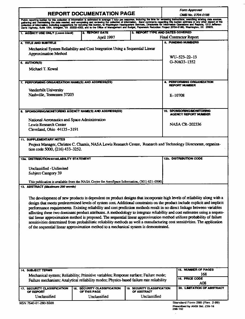
Fo.. Aoprove_REPORT DOCUMENTATION PAGE oMeNoo7o_o1_
l=ublk=_ bu_eamlot_ co¢Imceea_ Inl(mnm_mk mtJmm=od_ _ i hourl_=fmponN. Inclu,_Irbomare_ lotmdmtnl) Inmmctloa_m.s4mn:hlnllm_ _ m.
¢=amm _ m,,mm. _ _ ,¢_ wmNn_e, Hemqeanm . DC 20e0_Davis Hlghmay. S_to 1204. Arlington.VA 22202-4302. and to the Ollim d Managenmntand Budget.Papemod( Rodudion Projea (070401118). Wath_.
1. AGENCY _ ONLY (Leave b/ank) 2. REPORT DATE & REPORT TYPE AND DATES CO_m_D
Alail 19974. TI1LE ,t.ND SI_11T_
Mechanical System Reliability and Cost Integration Using a Sequential LinearApproximation Method
e. _UTHOR(S)
Michael T. I_wal
7. PERFORMING Of IGAJNIIZATION NAME(S) AND ADDRr_ES)
Vanderbilt UniversityNashville, Tennessee 37203
9. SPONSORI_ORING AGENCY NAME(S) AND ADDRESS(ES)
National Aeronautics and Space AdministrationLewis Research CenterCleveland, Ohio 44135-3191
Final Contractor Report5. RINDU_ NIJI_EFIS
WU--523-22--13G-NAG3--1352
8. PERFORMING OFIGANIZA'DONREPOFIT NUMBP_q
E---10708
10. SPON_R)mNGnUCN41TORING
AGENCY REPORT NUMBER
NASA CR-202336
11. SUPPLEMENTARY NOTES
Project Manage=',Christos C. Chamis, NASA Lewis Research Center, Research and Technology Direct(rate, organiza-tion code 5000, (216) 433-3252.
121. DISTRIBUTION/AVAILABILI13' STATEMENT 12b. DISTRIBUTION CODE
Unclassified -Unlimited
Subject Category 39
This publicalion is available fi-om the NASA Centc'r for AeroSpace Information, (301) 621--0390
13. ABSTRACT(Max/mum 200 words)
The development of new products is dependent on product designs that incorporate high levels of reliability along with adesign that meets predetermined levels of system COSLAdditional constraints on the product include explicit and implicitperformance requirements. Existing reliability and cost prediction methods result in no direct linkage between variablesaffecting these two dominant product attributes. A methodology to integrate reliability and cost estimates using a sequen-tial linear approximation method is proposed. The sequential linear approximation method utilizes probability of failuresensitivities determined from probabilistic reliability methods as well a manufacturing cost sensitivities. The applicationof the sequential linear approximation method to a mechanical system is demonstrated.
14. SUBJECT TERMS
Mechanical system; Reliability; Primitive variables; Re_m._ surface; Failure mode;Failure mechanism; Analytical reliability modes; Physics-based failure rate reliability
17. SECURITY CLASSIFICATIONOF REPORT
Unclassified
NSN 7540-0%280-5500
18. SECURITY CLASSIFICATIONOF THIS PAGE
Unclassified
19. SECURITY CLASSIFICATIONOF ABSTRACT
Unclassified
15. NUMBEROFPAGES
16816. PPJCE COOE
A0820. uMrrATION OF ABSTRACT
Standard Form 298 (Rev. 2-89)
Presori3ed by ANSI Std. Z39-18298-102