Matrix Stiffness Method 1011

Structural Analysis IV

Matrix Stiffness Method

4th Year

Structural Engineering

2010/11

Dr. Colin Caprani

Dr. C. Caprani 1


Contents

1. Introduction ......................................................................................................... 4

1.1 Background...................................................................................................... 4

1.2 Basic Concepts................................................................................................. 5

1.3 Matlab Truss Analysis Program ...................................................................... 7

2. Basic Approach.................................................................................................... 9

2.1 Individual Element .......................................................................................... 9

2.2 Assemblies of Elements................................................................................. 11

2.3 Example 1 ...................................................................................................... 13

2.4 General Methodology .................................................................................... 19

2.5 Member contribution to global stiffness matrix ............................................ 21

2.6 Interpretation of Stiffness Matrix .................................................................. 26

2.7 Restricting a Matrix ....................................................................................... 28

3. Plane Trusses ..................................................................................................... 31

3.1 Introduction.................................................................................................... 31

3.2 Truss Element Stiffness Matrix ..................................................................... 34

3.3 Element Forces .............................................................................................. 39

3.4 Example 2: Basic Truss ................................................................................. 42

3.5 Example 3: Adding Members........................................................................ 51

3.6 Example 4: Using Symmetry......................................................................... 55

3.7 Self-Strained Structures................................................................................. 58

3.8 Example 5 – Truss with Differential Temperature........................................ 62

3.9 Example 6 – Truss with Loads & Self Strains .............................................. 68

3.10 Problems..................................................................................................... 73

4. Beams.................................................................................................................. 75

4.1 Beam Element Stiffness Matrix..................................................................... 75

4.2 Beam Element Loading ................................................................................. 80

4.3 Example 7 – Simple Two-Span Beam........................................................... 82

Dr. C. Caprani 2


4.4 Example 8 – Non-Prismatic Beam ................................................................ 86

4.5 Problems ........................................................................................................ 90

5. Plane Frames...................................................................................................... 92

5.1 Plane Frame Element Stiffness Matrix.......................................................... 92

5.2 Example 9 – Simple Plane Frame ............................................................... 101

5.3 Example 10 –Plane Frame Using Symmetry .............................................. 106

5.4 Problems ...................................................................................................... 112

6. Appendix .......................................................................................................... 114

6.1 Plane Truss Element Stiffness Matrix in Global Coordinates..................... 114

6.2 Coordinate Transformations ........................................................................ 123

6.3 Past Exam Questions ................................................................................... 131

7. References ........................................................................................................ 141

Dr. C. Caprani 3


1. Introduction

1.1 Background

The matrix stiffness method is the basis of almost all commercial structural analysis

programs. It is a specific case of the more general finite element method, and was in

part responsible for the development of the finite element method. An understanding

of the underlying theory, limitations and means of application of the method is

therefore essential so that the user of analysis software is not just operating a ‘black

box’. Such users must be able to understand any errors in the modelling of structures

which usually come as obtuse warnings such as ‘zero pivot’ or ‘determinant zero:

structure unstable: aborting’. Understanding the basics presented herein should

hopefully lead to more fruitful use of the available software.

Note: LinPro is very useful as a study aid for this topic: right click on a member and

select “Stiffness Matrix” to see the stiffness matrix for any member.

Dr. C. Caprani 4


1.2 Basic Concepts

Node

The more general name for a connection between adjacent members is termed a node.

For trusses and frames the terms joint and node are interchangeable. For more

complex structures (e.g. plates), they are not.

Element

For trusses and frames element means the same as member. For more complex

structures this is not the case.

Degree of Freedom

The number of possible directions that displacements or forces at a node can exist in

is termed a degree of freedom (dof). Some examples are:

Plane truss: has 2 degrees of freedom at each node: translation/forces in the x and y

directions.

Beams: have 2 degrees of freedom per node: vertical displacement/forces and

rotation/moment.

Plane Frame: has 3 degrees of freedom at each node: the translations/forces similar

to a plane truss and in addition, the rotation or moment at the joint.

Space Truss: a truss in three dimensions has 3 degrees of freedom: translation or

forces along each axis in space.

Space Frame: has 6 degrees of freedom at each node: translation/forces along each

axis, and rotation/moments about each axis.

Dr. C. Caprani 5


Thus a plane truss with 10 joints has 20 degrees of freedom. A plane frame with two

members will have three joints (one common to both members) and thus 9 degrees of

freedom in total.

Local and Global

Forces, displacements and stiffness matrices are often derived and defined for an axis

system local to the member. However there will exist an overall, or global, axis

system for the structure as a whole. We must therefore transform forces,

displacements etc from the local coordinate system into the global coordinate system.

Dr. C. Caprani 6


1.3 Matlab Truss Analysis Program

Description

To support the ideas developed here we will introduce some Matlab scripts at each

point to demonstrate how the theory described can be implemented for computer

calculation. This collection of scripts will build into a program that can analyse pin-

jointed trusses. The scripts will only demonstrate the calculations process, and do not

have any graphical user interface facilities. This keeps the calculation process

unencumbered by extra code. (In fact probably 90+% of code in commercial

programs is for the graphical user interface and not for the actual calculations

process.) Of course, this is not to say that graphical displays of results are

unimportant; gross mistakes in data entry can sometimes only be found with careful

examination of the graphical display of the input data.

The scripts that are developed in these notes are written to explain the underlying

concepts, and not to illustrate best programming practice. The code could actually be

a lot more efficient computationally, but this would be at cost to the clarity of

calculation. In fact, a full finite element analysis program can be implemented in

under 50 lines (Alberty et al, 1999)!

It is necessary to use a scripting language like Matlab, rather than a spreadsheet

program (like MS Excel) since the number of members and member connectivity can

change from structure to structure.

The program will be able to analyse plane pin-jointed-trusses subject to nodal loads

only. It will not deal with member prestress, support stiffness or lack of fits: it is quite

rudimentary on purpose.

Dr. C. Caprani 7


Use

To use the program, download it from the course website (www.colincaprani.com).

Extract the files to a folder and change the current Matlab directory to that folder.

After preparing the data (as will be explained later), execute the following statement

at the command line:

>> [D F R] = AnalyzeTruss(nData,eData)

This assumes that the nodal data is stored in the matrix nData, and the element data

matrix is stored in eData – these names are arbitrary. Entering the required data into

Matlab will also be explained later.

Dr. C. Caprani 8

http://www.colincaprani.com/


Dr. C. Caprani 9

2. Basic Approach

2.1 Individual Element

We consider here the most basic form of stiffness analysis. We represent a structural

member by a spring which has a node (or connection) at each end. We also consider

that it can only move in the x-direction. Thus it only has 1 DOF per node. At each of

its nodes, it can have a force and a displacement (again both in the x-direction):

Notice that we have drawn the force and displacement vector arrows in the positive x-

direction. Matrix analysis requires us to be very strict in our sign conventions.

Using the basic relationship that force is equal to stiffness times displacement, we can

determine the force at node 1 as:

1 net displacement at 1F k

Thus:

1 1 2 1F k u u ku ku 2 (2.1)

Similarly for node 2:

2 2 1 1F k u u ku ku 2 (2.2)


Dr. C. Caprani 10

We can write equations (2.1) and (2.2) in matrix form to get the element stiffness

matrix for a 1-DOF axial element:

(2.3) 1

2 2

F uk k

F uk k

1

Ands using matrix notation, we write:

e F k ue (2.4)

Here:

eF is the element force vector;

k is the element stiffness matrix;

eu is the element displacement vector.

It should be clear that the element stiffness matrix is of crucial importance – it links

nodal forces to nodal displacements; it encapsulates how the element behaves under

load.

The derivation of the element stiffness matrix for different types of elements is

probably the most awkward part of the matrix stiffness method. However, this does

not pose as a major disadvantage since we only have a few types of elements to

derive, and once derived they are readily available for use in any problem.


Dr. C. Caprani 11

2.2 Assemblies of Elements

Real structures are made up of assemblies of elements, thus we must determine how

to connect the stiffness matrices of individual elements to form an overall (or global)

stiffness matrix for the structure.

Consider the following simple structure:

Note that the individual elements have different stiffnesses, and . Thus we can

write the force displacement relationships for both elements as:

1k 2k

(2.5) 1 1 1

2 1 1

F k k u

F k k u

1

2

2

1

2

(2.6) 2 2 2

3 32 2

F uk k

F uk k

We can expand these equations so that they encompass all the nodes in the structure:

1 1 1

2 1 1

3 3

0

0

0 0 0

F k k u

F k k u

F u

(2.7)

(2.8) 1 1

2 2 2

3 2 2

0 0 0

0

0

F u

F k k

F k k

2

3

u

u


Dr. C. Caprani 12

We can add equations (2.7) and (2.8) to determine the total of both the forces and

displacements at each node in the structure:

1 1 1

2 1 1 2 2

3 2 2

0

0

F k k u

F k k k k u

F k k

1

2

3u

2

(2.9)

As can be seen from this equation, by adding, we have the total stiffness at each node,

with contributions as appropriate by each member. In particular node 2, where the

members meet, has total stiffness 1k k . We can re-write this equation as:

F K u (2.10)

In which:

F is the force vector for the structure;

K is the global stiffness matrix for the structure;

u is the displacement vector for the structure.


2.3 Example 1

Problem

The following axially-loaded structure has loads applied as shown:

The individual member properties are:

Member Length (m) Area (mm2) Material, E (kN/mm2)

1 0.28 400 70

2 0.1 200 100

3 0.1 70 200

Find the displacements of the connections and the forces in each member.

Dr. C. Caprani 13


Dr. C. Caprani 14

Solution

Our first step is to model the structure with elements and nodes, as shown:

Calculate the spring stiffnesses for each member:

3

1

1

70 400100 10 kN/m

0.28

EAk

L

(2.11)

3

2

2

100 200200 10 kN/m

0.1

EAk

L

(2.12)

3

3

3

200 70140 10 kN/m

0.1

EAk

L

(2.13)

Next we calculate the individual element stiffness matrices:

(2.14) 1 3

2 2

100 10010

100 100

F u

F u

1

2 (2.15) 2 3

3 3

200 20010

200 200

F u

F u


Dr. C. Caprani 15

(2.16) 3 3

4 4

140 14010

140 140

F u

F u

3

We expand and add the element stiffness matrices to get:

(2.17)

1 1

2 23

3 3

4 4

100 100 0 0

100 100 200 200 010

0 200 200 140 140

0 0 140 140

F u

F u

F u

F u

Notice how each member contributes to the global stiffness matrix:

Node 1 Node 2 Node 3 Node 4

Node 1

0 0

Node 2 0

Node 3 0

Node 4 0 0

Notice also that where the member stiffness matrices overlap in the global stiffness

matrix that the components (or entries) are added. Also notice that zeros are entered

where there is no connection between nodes, e.g. node 1 to node 3.


Dr. C. Caprani 16

We cannot yet solve equation (2.17) as we have not introduced the restraints of the

structure: the supports at nodes 1 and 4. We must modify equation (2.17) in such a

way that we will obtain the known results for the displacements at nodes 1 and 4.

Thus:

1

22 3

33

4

0 1 0 0 0

0 100 200 200 010

0 200 200 140 0

0 0 0 0 1

u

uF

uF

u

2

(2.18)

What we have done here is to ‘restrict’ the matrix: we have introduced a 1 on the

diagonal of the node number, and set all other entries on the corresponding row and

column to zero. We have entered the known displacement as the corresponding entry

in force vector (zero). Thus when we now solve we will obtain . 1 4 0u u

For the remaining two equations, we have:

(2.19) 2 3

3 3

300 20010

200 340

F u

F u

And so:

2 3

33

340 200 50 31 1 110 m

200 300 100 2010 300 340 200 200 62

0.048 mm

0.322

u

u

(2.20)

To find the forces in the bars, we can now use the member stiffness matrices, since

we know the end displacements:


Dr. C. Caprani 17

Member 1

(2.21) 1 3

2

100 100 0 4.810 10

100 100 0.048 4.8

F

F

3

Thus Member 1 has a tension of 4.8 kN, since the directions of the member forces are

interpreted by our sign convention:

Also note that it is in equilibrium (as we might expect).

Member 2

(2.22) 2 3

3

200 200 0.048 54.810 10

200 200 0.322 54.8

F

F

3

3

Member 2 thus has tension of 54.8 kN.

Member 3

(2.23) 3 3

4

140 140 0.322 45.0810 10

140 140 0 45.08

F

F

Thus Member 3 has a compression of 45.08 kN applied to it.


Problem

Find the displacements of the connections and the forces in each member for the

following structure:

Dr. C. Caprani 18


2.4 General Methodology

Steps

The general steps in Matrix Stiffness Method are:

1. Calculate the member stiffness matrices

2. Assemble the global stiffness matrix

3. Restrict the global stiffness matrix and force vector

4. Solve for the unknown displacements

5. Determine member forces from the known displacements and member stiffness

matrices

6. Determine the reactions knowing member end forces.

Dr. C. Caprani 19


Matlab Program - Implementation

These steps are implemented in the Matlab Program as follows:

function [D F R] = AnalyzeTruss(nData,eData) % This function analyzes the truss defined by nData and eData: % nData = [x, y, xLoad, yLoad, xRestraint, yRestraint] % eData = [iNode, jNode, E, A]; kg = AssembleTrussK(nData, eData); % Assemble global stiffness matrix fv = AssembleForceVector(nData); % And the force vector [kgr fv] = Restrict(kg, fv, nData); % Impose restraints D = fv/kgr; % Solve for displacements F = ElementForces(nData,eData,D); % Get the element forces R = D*kg; % Get the reactions

The output from the function AnalyzeTruss is:

D: vector of nodal deflections;

F: vector of element forces;

R: vector of nodal forces (indicating the reactions and applied loads).

The input data required (nData and eData) will be explained later.

Dr. C. Caprani 20


2.5 Member contribution to global stiffness matrix

Consider a member, ij, which links node i to node j. Its member stiffness matrix will

be:

Node i Node j

Node i k11ij k12ij

Node j k21ij k22ij

Its entries must then contribute to the corresponding entries in the global stiffness

matrix:

… Node i … Node j …

… … … … … …

Node i … k11ij … k12ij …

… … … … … …

Node j … k21ij … k22ij …

… … … … … …

If we now consider another member, jl, which links node j to node l. Its member

stiffness matrix will be:

Dr. C. Caprani 21


Node j Node l

Node j k11jl k12jl

Node l k21jl k22jl

And now the global stiffness matrix becomes:

… Node i … Node j … Node l …

… … … … … … … …

Node i … k11ij … k12ij … … …

… … … … … … … …

Node j … k21ij … k22ij + k11jl

… k12jl …

… … … … … … … …

Node l … … k21lj … k22jl …

… … … … … … … …

In the above, the identifiers k11 etc are sub-matrices of dimension:

ndof × ndof

where ndof refers to the number of degrees of freedom that each node has.

Dr. C. Caprani 22


Matlab Program – Element Contribution

Considering trusses, we have 2 degrees of freedom (DOFs) per node, the x direction

and the y direction. Thus, for a truss with nn number of nodes, there are 2nn DOFs in

total. The x-DOF for any node i is thus located at 2i-1 and the y-DOF at 2i.

Consider a truss member connecting nodes i and j. To add the 4×4 truss element

stiffness matrix into the truss global stiffness matrix, we see that each row adds into

the following matrix columns:

2i-1 2i 2j-1 2j

The rows in the global stiffness matrix corresponding to the rows of the element

stiffness matrix are:

1. Row 1: Adds to row 2i-1 of the global stiffness matrix;

2. Row 2: Adds to row 2i;

3. Row 3: adds to row 2j-1;

4. Row 4: adds to row 2j.

Note of course that the column and row entries occur in the same order.

These rules are implemented for our Truss Analysis Program as follows:

function kg = AddElement(iEle,eData,ke,kg) % This function adds member iEle stiffness matrix ke to the global % stiffness matrix kg. % What nodes does the element connect to? iNode = eData(iEle,1); jNode = eData(iEle,2); % The DOFs in kg to enter the properties into DOFs = [2*iNode-1 2*iNode 2*jNode-1 2*jNode]; % For each row of ke for i = 1:4 % Add the row to the correct entries in kg kg(DOFs(i),DOFs) = kg(DOFs(i),DOFs) + ke(i,:); end

Dr. C. Caprani 23


Matlab Program – Global Stiffness Matrix Assembly

The function that assembles the truss global stiffness matrix for the truss is as

follows:

function kg = AssembleTrussK(nData, eData) % This function assembles the global stiffness matrix for a truss from the % joint and member data matrices % How many nodes and elements are there? [ne ~] = size(eData); [nn ~] = size(nData); % Set up a blank global stiffness matrix kg = zeros(2*nn,2*nn); % For each element for i = 1:ne E = eData(i,3); % Get its E and A A = eData(i,4); [L c s] = TrussElementGeom(i,nData,eData); % Geometric Properties ke = TrussElementK(E,A,L,c,s); % Stiffness matrix kg = AddElement(i,eData,ke,kg); % Enter it into kg end

Note that we have not yet covered the calculation of the truss element stiffness

matrix. However, the point here is to see that each element stiffness matrix is

calculated and then added to the global stiffness matrix.

Dr. C. Caprani 24


Matlab Program – Force Vector

Examine again the overall equation (2.10) to be solved:

F K u

We now have the global stiffness matrix, we aim to calculate the deflections thus we

need to have a force vector representing the applied nodal loads. Again remember

that each node as two DOFs (x- and y-loads). The code for the force vector is thus:

function f = AssembleForceVector(nData) % This function assembles the force vector % How may nodes are there? [nn ~] = size(nData); % Set up a blank force vector f = zeros(1,2*nn); % For each node for i = 1:nn f(2*i - 1) = nData(i, 3); % x-load into x-DOF f(2*i) = nData(i, 4); % y-load into y-DOF end

Dr. C. Caprani 25


Dr. C. Caprani 26

2.6 Interpretation of Stiffness Matrix

It is useful to understand what each term in a stiffness matrix represents. If we

consider a simple example structure:

We saw that the global stiffness matrix for this is:

11 12 13 1 1

21 22 23 1 1 2 2

31 32 33 2 2

0

0

K K K k k

K K K k k k k

K K K k k

K

If we imagine that all nodes are fixed against displacement except for node 2, then we

have the following:


Dr. C. Caprani 27

From our general equation:

(2.24) 1 11 12 13 1

2 21 22 23 2

3 31 32 33 3

0

1

0

F K K K K

F K K K K

F K K K K

2

2

2

2

Thus:

1 12 1

2 22 1

3 32 2

F K k

F K k k

F K k

(2.25)

These forces are illustrated in the above diagram, along with a free-body diagram of

node 2.

Thus we see that each column in a stiffness matrix represents the forces required to

maintain equilibrium when the column’s DOF has been given a unit displacement.

This provides a very useful way to derive member stiffness matrices.


Dr. C. Caprani 28

2.7 Restricting a Matrix

In Example 1 we solved the structure by applying the known supports into the global

stiffness matrix. We did this because otherwise the system is unsolvable; technically

the determinant of the stiffness matrix is zero. This mathematically represents the fact

that until we apply boundary conditions, the structure is floating in space.

To impose known displacements (i.e. supports) on the structure equations we modify

the global stiffness matrix and the force vector so that we get back the zero

displacement result we know.

Considering our two-element example again, if node 1 is supported, . Consider

the system equation:

1 0u

(2.26) 1 11 12 13

2 21 22 23

3 31 32 33

F K K K u

F K K K u

F K K K u

1

2

3

2

3

u

u

Therefore to obtain from this, we change K and F as follows: 1 0u

(2.27) 1

2 22 23

3 32 33

0 1 0 0

0

0

u

F K K

F K K

Now when we solve for we will get the answer we want: 1u 1 0u . In fact, since we

now do not need this first equation, we could just consider the remaining equations:

(2.28) 2 22 23

3 32 33

F K K u

F K K u

2

3


And these are perfectly solvable.

Thus to summarize:

To impose a support condition at degree of freedom i:

1. Make the force vector element of DOF i zero;

2. Make the i column and row entries of the stiffness matrix all zero;

3. Make the diagonal entry ,i i of the stiffness matrix 1.

Dr. C. Caprani 29


Matlab Program – Imposing Restraints

To implement these rules for our Truss Analysis Program, we will first create of

vector which tells us whether or not a DOF is restrained. This vector will have a zero

if the DOF is not restrained, and a 1 if it is.

Once we have this vector of restraints, we can go through each DOF and modify the

force vector and global stiffness matrix as described before. The implementation of

this is as follows:

function [kg f] = Restrict(kg, f, nData) % This function imposes the restraints on the global stiffness matrix and % the force vector % How may nodes are there? [nn ~] = size(nData); % Store each restrained DOF in a vector RestrainedDOFs = zeros(2*nn,1); % For each node, store if there is a restraint for i = 1:nn % x-direction if nData(i,5) ~= 0 % if there is a non-zero entry (i.e. supported) RestrainedDOFs(2*i-1) = 1; end % y-direction if nData(i,6) ~= 0 % if there is a support RestrainedDOFs(2*i) = 1; endend % for each DOF for i = 1:2*nn if RestrainedDOFs(i) == 1 % if it is restrained f(i) = 0; % Ensure force zero at this DOF kg(i,:) = 0; % make entire row zero kg(:,i) = 0; % make entire column zero kg(i,i) = 1; % put 1 on the diagonal end end

Dr. C. Caprani 30


3. Plane Trusses

3.1 Introduction

Trusses are assemblies of members whose actions can be linked directly to that of the

simple spring studied already:

EA

kL

(3.1)

There is one main difference, however: truss members may be oriented at any angle

in the xy coordinate system (Cartesian) plane:

Thus we must account for the coordinate transformations from the local member axis

system to the global axis system.

Dr. C. Caprani 31


Matlab Program – Data Preparation

In the following sections we will put the final pieces of code together for our Truss

Analysis Program. At this point we must identify what information is required as

input to the program, and in what format it will be delivered.

The node data is stored in a matrix nData. Each node of the truss is represented by a

row of data. In the row, we put the following information in consecutive order in

columns:

1. x-coordinate;

2. y-coordinate;

3. x-load: 0 or the value of load;

4. y-load: 0 or the value of load;

5. x-restraint: 0 if unrestrained, any other number if restrained;

6. y-restraint: 0 if unrestrained, any other number if restrained.

The element data is stored in a matrix called eData. Each element has a row of data

and for each element the information stored in the columns in order is:

1. i-Node number: the node number at the start of the element;

2. j-Node number: the other node the element connects to;

3. E: the Modulus of Elasticity of the element material;

4. A: the element area;

We will prepare input data matrices in the above formats for some of the examples

that follow so that the concepts are clear. In doing so we keep the units consistent:

Dimensions are in m;

Forces in kN

Elastic modulus is in kN/mm2;

Area is mm2.

Dr. C. Caprani 32


Matlab Program – Data Entry

To enter the required data, one way is:

1. Create a new variable in the workspace (click on New Variable);

2. Name it eData for example;

3. Double click on the new variable to open the Matlab Variable Editor;

4. Enter the necessary input data (can paste in from MS Excel, or type in);

5. Repeat for the nodal data.

Dr. C. Caprani 33


Dr. C. Caprani 34

3.2 Truss Element Stiffness Matrix

For many element types it is very difficult to express the element stiffness matrix in

global coordinates. However, this is not so for truss elements. Firstly we note that the

local axis system element stiffness matrix is given by equation (2.3):

1 1

1 1

k kk

k k

k

(3.2)

Next, introducing equation (3.1), we have:

1 1

1 1

EA

L

k (3.3)

However, this equation was written for a 1-dimensional element. Expanding this to a

two-dimensional axis system is straightforward since there are no y-axis values:

1 0 1 0

0 0 0 0

1 0 1 0

0 0 0 0

i

i

j

j

x

yEAxL

y

k

(3.4)

Next, using the general element stiffness transformation equation (See the Appendix):

Tk = T k T (3.5)

And noting the transformation matrix for a plane truss element from the Appendix:


Dr. C. Caprani 35

cos sin 0 0

sin cos 0 0

0 0 cos sin

0 0 sin cos

P

P

T 0T =

0 T (3.6)

We have:

1cos sin 0 0 1 0 1 0

sin cos 0 0 0 0 0 0

0 0 cos sin 1 0 1 0

0 0 sin cos 0 0 0 0

cos sin 0 0

sin cos 0 0

0 0 cos sin

0 0 sin cos

EA

L

k

(3.7)

Carrying out the multiplication gives:

2 2

2 2

2 2

2 2

cos cos sin cos cos sin

cos sin sin cos sin sin



EA

L

k (3.8)

If we examine the nodal sub-matrices and write cosc , sins :

2 2

2 2

2 2

2 2

c cs c cs

cs s cs sEA

L c cs c cs

cs s cs s

k (3.9)


Labelling the nodal sub-matrices as:

k11 k12k

k21 k22 (3.10)

Then we see that the sub-matrices are of dimension 2 × 2 (No. DOF × No. DOF) and

are:

2

2

c csEA

L cs s

k11 (3.11)

And also note:

(3.12) k11 = k22 = -k12 = -k21

Therefore, we need only evaluate a single nodal sub-matrix ( ) in order to find the

total element stiffness matrix in global coordinates.

k11

Dr. C. Caprani 36


Matlab Program – Element Stiffness Matrix

Calculating the element stiffness matrix for our Truss Analysis Program is easy. The

only complexity is extracting the relevant data from the input node and element data

matrices. Rather than try determine the angle that the truss member is at (remember

we only have the nodal coordinates), we can calculate cos and sin directly (e.g.

adjacent/hypotenuse). Further, the element length can be found using Pythagoras,

given the nodal coordinates. These element properties are found in the script below:

function [L c s] = TrussElementGeom(iEle,nData,eData); % This function returns the element length % What nodes does the element connect to? iNode = eData(iEle,1); jNode = eData(iEle,2); % What are the coordinates of these nodes? iNodeX = nData(iNode,1); iNodeY = nData(iNode,2); jNodeX = nData(jNode,1); jNodeY = nData(jNode,2); % Use Pythagoras to work out the member length L = sqrt((jNodeX - iNodeX)^ 2 + (jNodeY - iNodeY)^ 2); % Cos is adjacent over hyp, sin is opp over hyp c = (jNodeX - iNodeX)/L; s = (jNodeY - iNodeY)/L;

The E and A values for each element are directly found from the input data element

matrix as follows:

E = eData(i,3); % Get its E and A A = eData(i,4);

Thus, with all the relevant data assembled, we can calculate the truss element

stiffness matrix. In the following Matlab function, note that we make use of the fact

that each nodal sub-matrix can be determined from the nodal sub-matrix k1 : 1

Dr. C. Caprani 37


function k = TrussElementK(E,A,L,c,s) % This function returns the stiffness matrix for a truss element k11 = [ c^2 c*s; c*s s^2]; k = (E*A/L) * [ k11 -k11; -k11 k11];

Dr. C. Caprani 38


Dr. C. Caprani 39

3.3 Element Forces

The forces applied to a member’s ends are got from the element equation:

e F k ue

i

(3.13)

Expanding this in terms of nodal equations we have:

i

j j

F δk11 k12

F δk21 k22 (3.14)

Thus we know:

j i j F k21 δ k22 δ (3.15)

From which we could determine the member’s axial force. However, for truss

members, we can determine a simple expression to use if we consider the change in

length in terms of the member end displacements:

x jx ixL (3.16)

y jyL iy (3.17)

And using the coordinate transforms idea:

cos sinx yL L L (3.18)

Also we know that the member force is related to the member elongation by:


Dr. C. Caprani 40

EA

F LL

(3.19)

Thus we have:

cos sinx y

EAF L L

L (3.20)

And introducing equations (3.16) and (3.17) gives:

cos sin jx ix

jy iy

EAF

L

(3.21)

A positive result from this means tension and negative compression.


Matlab Program – Element Force

Once the element nodal deflections are known, the element forces are found as

described above. Most of the programming effort is dedicated to extracting the nodal

deflections that are relevant for the particular member under consideration:

function F = TrussElementForce(nData, eData, d, iEle) % This function returns the element force for iEle given the global % displacement vector, d, and the node and element data matrices. % What nodes does the element connect to? iNode = eData(iEle,1); jNode = eData(iEle,2); % Get the element properties E = eData(iEle,3); % Get its E and A A = eData(iEle,4); [L c s] = TrussElementGeom(iEle,nData,eData); % Geometric Properties dix = d(2*iNode-1); % x-displacement at node i diy = d(2*iNode); % y-displacement at node i djx = d(2*jNode-1); % x-displacement at node j djy = d(2*jNode); % y-displacement at node j F = (E*A/L) * (c*(djx-dix) + s*(djy-diy));

Note also that the way the program is written assumes that tension is positive and

compression is negative. We also want to return all of the element forces, so we use

the function just described to calculate all the truss elements’ forces:

function F = ElementForces(nData,eData,d) % This function returns a vector of the element forces % How many elements are there? [ne ~] = size(eData); % Set up a blank element force vector F = zeros(ne,1); % For each element for i = 1:ne % Get its force and enter into vector F(i) = TrussElementForce(nData, eData, d, i); end

Dr. C. Caprani 41


3.4 Example 2: Basic Truss

Problem

Analyse the following truss using the stiffness matrix method.

Note that:

2200 kN/mmE ;

The reference area is 2 . 100mmA

Dr. C. Caprani 42


Dr. C. Caprani 43

Solution

STEP 1: Determine the member stiffness matrices:

Member 12

The angle this member makes to the global axis system and the relevant values are:

21 1cos cos45

22c c

21 1sin sin 45

2 22s s 1

cs

Therefore:

2

12 212

0.5 0.5200 100 2

0.5 0.510 2

c csEA

L cs s

k11

Thus:

3

12

0.5 0.510

0.5 0.5

k11 (3.22)

Notice that the matrix is symmetrical as it should be.


Dr. C. Caprani 44

Member 23

The angle this member makes to the global axis system and the relevant values are:

21 1cos cos315

22c c

21 1sin sin315

2 22s s 1

cs

Therefore:

2

23 223

0.5 0.5200 100 2

0.5 0.510 2

c csEA

L cs s

k11

Thus:

3

23

0.5 0.510

0.5 0.5

k11 (3.23)

Again the matrix is symmetrical.


Dr. C. Caprani 45

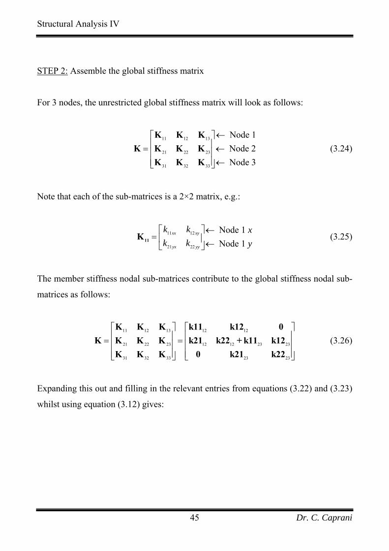
STEP 2: Assemble the global stiffness matrix

For 3 nodes, the unrestricted global stiffness matrix will look as follows:

11 12 13

21 22 23

31 32 33

Node 1

Node 2

Node 3

K K K

K K K K

K K K

(3.24)

Note that each of the sub-matrices is a 2×2 matrix, e.g.:

11 12

21 22

Node 1

Node 1 xx xy

yx yy

k k x

k k y

11K (3.25)

The member stiffness nodal sub-matrices contribute to the global stiffness nodal sub-

matrices as follows:

(3.26) 11 12 13 12 12

21 22 23 12 12 23 23

31 32 33 23 23

K K K k11 k12 0

K K K K k21 k22 + k11 k12

K K K 0 k21 k22

Expanding this out and filling in the relevant entries from equations (3.22) and (3.23)

whilst using equation (3.12) gives:


Dr. C. Caprani 46

3

0.5 0.5 0.5 0.5 0 0

0.5 0.5 0.5 0.5 0 0

0.5 0.5 1 0 0.5 0.510

0.5 0.5 0 1 0.5 0.5

0 0 0.5 0.5 0.5 0.5

0 0 0.5 0.5 0.5 0.5

K (3.27)

STEP 3: Write the solution equation in full

F = K δ (3.28)

Thus, keeping the nodal sub-matrices identifiable for clarity:

1 1

1 1

23

2

3 3

3 3

0.5 0.5 0.5 0.5 0 0

0.5 0.5 0.5 0.5 0 0

0 0.5 0.5 1 0 0.5 0.510

100 0.5 0.5 0 1 0.5 0.5

0 0 0.5 0.5 0.5 0.5

0 0 0.5 0.5 0.5 0.5

x x

y y

x

y

x x

y y

R

R

R

R

(3.29)

In which we have noted:

1xR is the reaction at node 1 in the x-direction (and similarly for the others);

The force at node 2 is 0 in the x-direction and -100 kN (downwards) in the y-

direction.


Dr. C. Caprani 47

STEP 4: Restrict the equation.

Now we impose the boundary conditions on the problem. We know:

1 1 0x y since node 1 is pinned;

3 3 0x y again, since node 3 is pinned.

Thus equation (3.29) becomes:

1

1

23

2

3

3

0 1 0 0 0 0 0

0 0 1 0 0 0 0

0 0 0 1 0 0 010

100 0 0 0 1 0 0

0 0 0 0 0 1 0

0 0 0 0 0 0 1

x

y

x

y

x

y

(3.30)

Since both DOFs are restricted for nodes 1 and 3, we can thus write the remaining

equations for node 2:

23

2

0 1 010

100 0 1x

y

(3.31)

STEP 5: Solve the system

The y-direction is thus the only active equation:

3

2100 10 y (3.32)

Thus:

2 0.1 m 100 mmy (3.33)


Dr. C. Caprani 48

STEP 6: Determine the member forces

For truss member’s we outlined a simple method encompassed in equation (3.21). In

applying this to Member 12 we note:

1 1 0x y since it is a support;

2 0x by solution;

2 0.1y again by solution.

Thus:

cos sin jx ix

jy iy

EAF

L

30 01 1 100

10 50 2 kN0.1 02 2 2

F

(3.34)

And so Member 12 is in compression, as may be expected. For Member 23 we

similarly have:

3

0 01 1 10010 50 2 kN

0 0.12 2 2F

(3.35)

And again Member 23 is in compression. Further, since the structure is symmetrical

and is symmetrically loaded, it makes sense that Member’s 12 and 23 have the same

force.

STEP 7: Determine the reactions

To determine the remaining unknown forces we can use the basic equation now that

all displacements are known:


1

1

3

3

3

0.5 0.5 0.5 0.5 0 0 0

0.5 0.5 0.5 0.5 0 0 0

0 0.5 0.5 1 0 0.5 0.5 010

100 0.5 0.5 0 1 0.5 0.5 0.1

0 0 0.5 0.5 0.5 0.5 0

0 0 0.5 0.5 0.5 0.5 0

x

y

x

y

R

R

R

R

(3.36)

Thus we have:

(3.37) 1

00.5 0.5 50kN

0.1xR

(3.38) 1

00.5 0.5 50kN

0.1yR

(3.39) 3

00.5 0.5 50kN

0.1xR

(3.40) 3

00.5 0.5 50kN

0.1yR

Again note that the sign indicates the direction along the global coordinate system.

We can now plot the full solution:

Dr. C. Caprani 49


Matlab Program – First Use

All necessary functions have been explained. The main function is given on page 20.

This also gives the single line of code that finds the reactions. The input data for the

example truss just given is:

Node Data Element Data

x y Fx Fy Rx Ry Node i Node j E A

0 0 0 0 1 1 1 2 200 70.71

10 10 0 -100 0 0 2 3 200 70.71

20 0 0 0 1 1

And the results from the program are:

Node DOF D R Element F

1 x 0 50 1 -70.71

y 0 50 2 -70.71

2 x 0 0

y -0.100 -100

3 x 0 -50

y 0 50

These results, of course, correspond to those found by hand.

The importance of the graphical display of the results should also be noted: there

could have been clear mistakes made in the preparation of the input data that would

not reveal themselves unless the physical interpretation of the results is appreciate by

drawing the deflected shape, the member forces, and the directions of the reactions.

Dr. C. Caprani 50


Dr. C. Caprani 51

3.5 Example 3: Adding Members

Problem

Analyse the truss of Example 2 but with the following member 14 added:

Solution

With the addition of node 4 we now know that the nodal sub-matrices global stiffness

equation will be 4×4 with the fully expanded matrix being 16×16. Rather than

determine every entry in this, let’s restrict it now and only determine the values we

will actually use. Since nodes 1, 3 and 4 are pinned, all their DOFs are fully restricted

out. The restricted equation thus becomes:

2 2F K22 δ (3.41)

Next we must identify the contributions from each member:

We already know the contributions of Members 12 and 23 from Example 2.

The contribution of Member 24 is to nodes 2 and 4. Since node 4 is restricted, we

only have the contribution 24k11 to K22 .

Thus K2 becomes: 2


Dr. C. Caprani 52

12 23 24 K22 k22 k11 k11 (3.42)

Next determine : this member makes an angle of 270° to the global axis system

giving:

24k11

2cos cos270 0 0c c

2sin sin 270 1 1 0s s cs

Therefore:

2

3

24 224

0 0 0 0200 1002 10

0 1 0 110

c csEA

L cs s

k11

Thus:

3

24

0 010

0 2

k11 (3.43)

Hence the global restricted stiffness matrix becomes:

(3.44) 3 3 31 0 0 0 1 0

10 10 100 1 0 2 0 3

K22

Writing the restricted equation, we have:

23

2

0 1 010

100 0 3x

y

(3.45)


Dr. C. Caprani 53

From which we find the only equation

3

2100 10 3 y (3.46)

Thus:

(3.47) 2 0.033 m 33.3 mmy

The member forces are:

3

12

0 01 110 23.6kN

0.033 02 2F

(3.48)

3

23

0 01 110 23.6kN

0 0.0332 2F

(3.49)

(3.50) 3

24

0 010 0 2 66.6kN

0.033 0F

Thus we have the following solution:


Matlab Program – Input/Output

The input data for this example is:

Node Data Element Data

x y Fx Fy Rx Ry Node i Node j E A

0 0 0 0 1 1 1 2 200 70.71

10 10 0 -100 0 0 2 3 200 70.71

20 0 0 0 1 1 2 4 200 100

10 0 0 0 1 1

The results are:

Node DOF D R Element F

1 x 0 16.66 1 -23.57

y 0 16.66 2 -23.57

2 x 0 0 3 66.66

y -0.033 -100

3 x 0 -16.66

y 0 16.66

4 x 0 0

y 0 66.66

Dr. C. Caprani 54


3.6 Example 4: Using Symmetry

Problem

Analyse the truss of Example 3 taking advantage of any symmetry:

Solution

Looking at the structure it is clear that by splitting the structure down the middle

along member 24 that we will have two equal halves:

Notice that we have changed the following:

Dr. C. Caprani 55


Dr. C. Caprani 56

The load is halved since it is now equally shared amongst two halves;

Similarly the area of member 24 is halved.

We now analyse this new truss as usual. However, we can make use of some previous

results. For Member 12:

3

12

0.5 0.510

0.5 0.5

k11 (3.51)

And for Member 24

3 3

24

0 0 0 0110 10

0 2 0 12

k11

(3.52)

Since the area is halved from that of Example 3, its stiffnesses are halved.

In restricting we note that the only possible displacement is node 2 in the y-direction.

However, we will keep using the node 2 sub-matrices until the last moment:

(3.53) 3 3 30.5 0 0 0 0.5 0

10 10 100 0.5 0 1 0 1.5

K22

Thus:

23

2

0 0.5 010

50 0 1.5x

y

(3.54)

And now imposing the boundary condition 2 0x :


Dr. C. Caprani 57

3

250 10 1.5 y (3.55)

From which we solve for the displacement:

3

2

2

50 10 1.5

0.033 m 33.3 mm

y

y

(3.56)

This (of course) is the same result we obtained in Example 3. For the member forces

we have:

3

12

0 01 110 23.6kN

0.033 02 2F

(3.57)

3

24

0 010 0 1 33.3kN

0 0.033F

(3.58)

Member 12 has the same force as per Example 3 as is expected.

It might appear that Member 24 has an erroneous force result. It must be remembered

that this is the force in the half-member (brought about since we are using symmetry).

Therefore the force in the full member is 2 33.3 66.6 kN as per Example 3.


3.7 Self-Strained Structures

Introduction

A self-strained structure is one where strains are induced by sources other than

externally applied loads. The two main examples are temperature difference and lack

of fit of a member. For example consider the effect if member 13 in the following

structure was too long and had to be ‘squeezed’ into place:

It should be intuitively obvious that to ‘squeeze’ the member into place a

compressive force was required to shorten it to the required length:

Dr. C. Caprani 58


Once the member has been put in place, the source of the ‘squeezing’ is removed.

Since the member wants to spring back to its original length, it pushes on its joints:

In this way members 12 and 14 will now go into tension whilst member 13 will

remain in compression, but a smaller compression than when it was ‘squeezed’ into

place since joint 1 will deflect to the right some amount.

In a similar way to lack of fit, examined above, if member 13 had been subject to a

temperature increase it would try to elongate. However this elongation is restrained

by the other members inducing them into tension and member 13 into some

compression.

Dr. C. Caprani 59


Dr. C. Caprani 60

Lack of Fit

We consider a member with original length of OL that is required to be of length

Req'dL . Thus a change in length of L must be applied:

Req'd OL L L (3.59)

Thus:

L is positive: the member is too short and must be lengthened to get into place;

L is negative, it is too long and must be shortened to get into place.

Thus we must apply a force to the member that will cause a change in length of L .

From basic mechanics:

OFLL

EA (3.60)

Thus the force required is:

O

LF EA

L

(3.61)

From the above sign convention for L :

F is positive when the member must be put into tension to get it in place;

F is negative when the member must be put into compression to get it in place.

Lastly, remember to apply the member force in opposite direction to the member’s

nodes.


Dr. C. Caprani 61

Temperature Change

We consider a member that is subject to a differential (i.e. different to the rest of the

structure) temperature change of T degrees Celsius. Also we must know the

coefficient of linear thermal expansion, , for the material. This is the change in

length, per unit length, per unit change in temperature:

O

LC

L

(3.62)

Thus the thermal strain induced in the member is:

T T (3.63)

And so the change in length is:

OL L T (3.64)

Also, since E , we find the force in the member:

T TF A EA T (3.65)

So finally, from equation (3.63), the force required to suppress the temperature

change is:

TF EA T (3.66)

Once again, apply this force in the opposite direction to the member’s nodes.


3.8 Example 5 – Truss with Differential Temperature

Problem

Member 13 of the following truss is subject to a temperature change of +100 °C.

Calculate the deflections of node 1 and the final forces in the members.

Take: 5 12 10 C ; 42 10 kNEA ; the area of member 12 as 2A; the area of

member 13 as A; and, the area of member 14 as A√2.

Dr. C. Caprani 62


Dr. C. Caprani 63

Solution

First we must recognize that there are two stages to the actions in the members:

Stage I: all displacements are suppressed and only the temperature force in

member 13 is allowed for;

Stage II: displacements are allowed and the actions of the temperature force in

member 13 upon the rest of the structure are analyzed for.

The final result is then the summation of these two stages:

The force induced in member 13 when displacements are suppressed is:

4 52 10 2 10 100

40kN

TF EA T

(3.67)


Dr. C. Caprani 64

Stage I

All displacements are suppressed. Thus:

1 0; 0x 1y (3.68)

(3.69) 12 13 140; ; 0I I

TF F F F I

Stage II

Displacements are allowed occur and thus we must analyse the truss. Using the

matrix stiffness method, and recognizing that only joint 1 can displace, we have:

1 1F K11 δ (3.70)

Also, since we cleverly chose the node numbers, the member contributions are just:

12 13 14 K11 k11 k11 k11 (3.71)

Member 12:

21 1cos cos120

2 4c c

23 3sin sin120

2 4s s 3

4cs

2 4

12 223

1 32 10 2 4 4

2.0 3 3

4 4

c csEA

L cs s

k11


Dr. C. Caprani 65

Member 13:

2cos cos180 1 1c c 2sin sin180 0 0 0s s cs

2 4

13 223

1 02 10

0 01.0

c csEA

L cs s

k11

Member 14:

21 1cos cos225

22c c

21 1sin sin 225

2 22s s 1

cs

42

14 223

2 10 2 0.5 0.5

0.5 0.51.0 2

c csEA

L cs s

k11

Thus from equation (3.71) we have:

4 7 2 32 10

4 2 3 5

K11 (3.72)

From the diagram for Stage II, we can see that the force applied to joint 1 is acting to

the right and so is positive. Thus:


Dr. C. Caprani 66

4

1

1

40 7 2 32 10

0 4 2 3 5

x

y

(3.73)

Solve this to get:

1

241

3

5 3 2 44 1

02 10 3 2 77 5 2 3

1.1510 m

0.06

x

y

0

(3.74)

Using equation (3.21) we can now find the member forces for Stage II:

4

3

12

0 1.152 10 2 1 310 12.54 kN

0 0.062.0 2 2IIF

(3.75)

43

13

0 1.152 101 0 10 23.0 kN

0 0.061.0IIF

(3.76)

4

3

14

2 10 2 0 1.151 110 15.4 kN

0 0.061.0 2 2 2IIF

(3.77)


Final

The final member forces are the superposition of Stage I and Stage II forces:

(3.78) 12 12 12 0 12.54 12.54 kNI IIF F F

(3.79) 13 13 13 40 23.0 17.0 kNI IIF F F

(3.80) 14 14 14 0 15.4 15.4 kNI IIF F F

Thus the final result is:

Dr. C. Caprani 67


3.9 Example 6 – Truss with Loads & Self Strains

Problem

Analyse the same truss as Example 5, allowing for the following additional load

sources:

80 kN acting horizontally to the left at node 1;

100 kN acting vertically downwards at node 1;

Member 14 is 5√2 mm too short upon arrival on site.

All as shown below:

Dr. C. Caprani 68


Dr. C. Caprani 69

Solution

Again we will separate the actions into Stage I and Stage II scenarios.

Stage I

Displacements are suppressed and as a result the only sources of forces are self-

straining forces:

The forces and displacements for Stage I are thus:

40kNTF as before,

3

4 5 2 102 2 10 100 2 kN

2L

LF EA

L

(3.81)

1 0; 0x 1y (3.82)

12 13 140; 40; 100 2I I IF F F (3.83)


Dr. C. Caprani 70

Stage II

In this stage displacements are allowed and the forces in the self-strained members

are now applied to the joints, in addition to any external loads. Thus we have:

Clearly we need to resolve the forces at node 1 into net vertical and horizontal forces:

Since the members have not changed from Example 5, we can use the same stiffness

matrix. Therefore we have :

4

1

1

140 7 2 32 10

200 4 2 3 5

x

y

(3.84)


Dr. C. Caprani 71

Solve this:

1

241

3

5 3 2 144 1

2002 10 3 2 77 5 2 3

3.710 m

7.8

x

y

0

(3.85)

Using equation (3.21) we can find the member forces for Stage II:

4

3

12

0 3.72 10 2 1 310 98.1 kN

0 7.82.0 2 2IIF

(3.86)

43

13

0 3.72 101 0 10 74.0 kN

0 7.81.0IIF

(3.87)

4

3

14

2 10 2 0 3.71 110 162.6 kN

0 7.81.0 2 2 2IIF

(3.88)


Final

As before, the final member forces are the Stage I and Stage II forces:

(3.89) 12 12 12 0 98.1 98.1 kNI IIF F F

(3.90) 13 13 13 40 74.0 114.0 kNI IIF F F

14 14 14 100 2 162.6 21.6 kNI IIF F F (3.91)

Thus the final result is:

Dr. C. Caprani 72


3.10 Problems

1. Determine the displacements of joint 1 and the member forces for the following

truss. Take 42 10 kNEA .

2. Determine the displacements of joint 1 and the member forces for the following

truss. Take 42 10 kNEA , the area of both members is A√2.

Ans. 1 5 mmx , 1 0y

Dr. C. Caprani 73


3. Using any pertinent results from Problem 3, determine the area of member 14

such that the horizontal displacement of node 1 is half what is was prior to the

installation of member 14. Determine also the force in member 14. Take 42 10 kNEA ,

Ans. 14A A , 14 50 kNF

Dr. C. Caprani 74


4. Beams

4.1 Beam Element Stiffness Matrix

To derive the beam element stiffness matrix, we recall some results obtained

previously, summarized here:

Next we must adopt strict local element sign convention and node identification:

Dr. C. Caprani 75


Anti-clockwise moments and rotations (i.e. from the x-axis to the y-axis) are positive

and upwards forces are positive.

Thus for a vertical displacement of at node i, now labelled iy , we have the

following ‘force’ vector:

3

2

3

2

12

6

12

6

iy

i

iy

jy

j

EI

LF EIM LF EI

LMEI

L

(4.1)

Similarly, applying the same deflection, but at node j, jy , gives:

3

2

3

2

12

6

12

6

iy

i

jy

jy

j

EI

LF EIM LF EI

LMEI

L

(4.2)

Next, applying a rotation to node i, i , gives:

Dr. C. Caprani 76


Dr. C. Caprani 77

2

2

6

4

6

2

iy

i

i

jy

j

EI

LF EIM LF EI

LMEI

L

(4.3)

And a rotation to node j, j , gives:

2

2

6

2

6

4

iy

i

j

jy

j

EI

LF EIM LF EI

LMEI

L

(4.4)

Since all of these displacement could happen together, using superposition we thus

have the total force vector as:

3 2 3 2

2 2

3 2 3

2 2

12 6 12 6

6 4 6 2

12 6 12 6

6 2 6 4

iy

i

iy i jy

jy

j

EI EI EI EI

L L L LF EI EI EI EIM L L L LF EI EI EI EI

L L L LMEI EI EI EI

L L L L

2

j

(4.5)

Writing this as a matrix equation, we have:


Dr. C. Caprani 78

3 2 3 2

2 2

3 2 3 2

2 2

12 6 12 6

6 4 6 2

12 6 12 6

6 2 6 4

iy iy

i i

jy jy

j j

EI EI EI EI

L L L LF EI EI EI EIM L L L LF EI EI EI EI

L L L LMEI EI EI EI

L L L L

(4.6)

This is in the typical form:

e F k ue (4.7)

And so the beam element stiffness matrix is given by:

3 2 3 2

2 2

3 2 3

2 2

12 6 12 6

6 4 6 2

12 6 12 6

6 2 6 4

2

EI EI EI EI

L L L LEI EI EI EI

L L L LEI EI EI EI

L L L LEI EI EI EI

L L L L

k (4.8)

Next we note a special case where the vertical displacements of the beam nodes are

prevented and only rotations of the beam ends is allowed. In this case, all terms

relating to the translation DOFs are removed giving us the reduced stiffness matrix

for a beam on rigid vertical supports:


Dr. C. Caprani 79

4 2

2 4

EI EI

L LEI EI

L L

k (4.9)

As we did for trusses, we will often write these equations in terms of nodal sub-

matrices as:

i i

j j

F δk11 k12

F δk21 k22 (4.10)


4.2 Beam Element Loading

Applied Loads

Beam loads are different to truss loads since they can be located anywhere along the

element, not only at the nodes – termed intermodal loading Beams can also have

loads applied to the nodes – nodal loading. We deal with these two kinds of loads as

follows:

Nodal loads: apply the load to the joint as usual;

Inter-nodal loads: apply the equivalent concentrated loads to the joints (these are

just fixed end moment reactions to the load, with the direction reversed).

If a member’s nodes are locked against rotation, the member end forces due to inter-

nodal loading will just be the fixed end moment and force reaction vector we are

familiar with FF . If a member also displaces, the total member end forces are:

Tot FF F k δ (4.11)

Thus the general stiffness equation becomes:

F K δ (4.12)

Where F is now the vector of net nodal loads:

Net Nodal Load Nodal Load Fixed End Reactions (4.13)

Dr. C. Caprani 80


Lastly, we must note that inter-nodal loads on adjacent members will result in

multiple loads on a node. Thus we must take the algebraic sum of the forces/moments

on each node in our analysis, bearing in mind the sign convention.

As an example, the equivalent nodal loads for a UDL applied to a beam element are:

Member End Forces

After the deformations of the beam are known, we can use the element stiffness

matrices to recover the end forces/moments on each element due to both

deformations and the inter-nodal loading directly from equation (4.11).

Dr. C. Caprani 81


Dr. C. Caprani 82

4.3 Example 7 – Simple Two-Span Beam

Problem

For the following beam, find the rotations of joints 2 and 3 and the bending moment

diagram. Take 3 26 10 kNmEI .

Solution

First we write the general equation in terms of nodal sub-matrices:

(4.14) 1 11 12 13

2 21 22 23

3 31 32 33

F K K K δ

F K K K δ

F K K K δ

1

2

3

1

2

3

Next we note that the only possible displacements are the rotations of joints 2 and 3.

Thus we can restrict the equation by eliminating joint 1 as follows:

(4.15) 1 11 12 13

2 21 22 23

3 31 32 33

F K K K δ

F K K K δ

F K K K δ

To give:


Dr. C. Caprani 83

(4.16) 2 22 23

3 32 33

F K K δ

F K K δ2

3

2

3

Since this beam is on rigid vertical supports, we can use the beam stiffness matrix

given by equation (4.9). Thus we are left with two equations:

2 22 23

3 32 33

M k k

M k k

(4.17)

The member contributions to each of these terms are:

; 22 Term 22 of Member 12 + Term 11 of Member 23k

; 23 Term 12 of Member 23k


33 Term 22 of Member 23k

Thus, for Member 12 we have:

3

12

4 6 2 64 24 26 610 10

2 4 2 42 6 4 6

6 6

EI EI

L LEI EI

L L

3

k (4.18)

And for Member 23:

3

23

4 6 2 64 26 610 102 42 6 4 6

6 6

3

k (4.19)


Dr. C. Caprani 84

Thus the global stiffness equation is:

2 3

3 3

8 210

2 4

M

M2

(4.20)

To find the moments to apply to the nodes, we determine the fixed-end moments

caused by the loads on each members. Only Member 23 has load, and its fixed end

moments are:

Our sign convention is anti-clockwise positive. Thus the moments to apply to the

joints become (refer to equation (4.13)):

23

3

30 8 210

30 2 4

(4.21)

Solving the equation:

2 3

33

4 2 30 90 141 110 rads

2 8 30 150 1410 8 4 2 2

(4.22)

Since we know that anti-clockwise is positive, we can draw the displaced shape (in

mrads):


Using the member stiffness matrices we can recover the bending moments at the end

of each member, now that the rotations are known, from equation (4.11):

1 3 3

2

0 4 2 0 12.910 10 kNm

0 2 4 90 14 25.7

M

M

(4.23)

2 3 3

3

30 4 2 90 14 25.710 10 kNm

30 2 4 150 14 0

M

M

(4.24)

Thus the final BMD can be drawn as:

Dr. C. Caprani 85


Dr. C. Caprani 86

4.4 Example 8 – Non-Prismatic Beam

Problem

For the following beam, find the vertical deflection of joint 2 and the bending

moment diagram. Take 3 212 10 kNmEI .

Solution

First we write the general equation in terms of nodal sub-matrices:

(4.25) 1 11 12 13

2 21 22 23

3 31 32 33

F K K K δ

F K K K δ

F K K K δ

1

2

3

Next we note that the only possible displacements are those of joint 2. Thus we can

restrict the equation to:

2 22 2F K δ (4.26)

The member contributions to are: 22K

Sub-matrix k22 of member 12;

Sub-matrix k11 of member 23.


Dr. C. Caprani 87

That is:

22 12 23 K k22 k11 (4.27)

For member 12, we have, from equation (4.8):

3 2 3 2

3 3

12

2 2

12 6 12 12 6 122.25 4.54 410 10

6 4 6 12 4 12 4.5 12

4 4

EI EI

L LEI EI

L L

k22 (4.28)

And for member 23:

3 2 3 2

3 3

23

2 2

12 6 12 24 6 244.5 94 410 10

6 4 6 24 4 24 9 2

4 4

EI EI

L LEI EI

L L

4

k11 (4.29)

Since the load is a directly applied nodal load we can now write equation (4.26),

using equations (4.27), (4.28), and (4.29), as:

2 3

2 2

100 6.75 4.510

0 4.5 36yF

M2 y

(4.30)

Solving:

2 3 3

2

36 4.5 100 16.16110 10

4.5 6.75 0 2.026.75 36 4.5 4.5y

(4.31)


Dr. C. Caprani 88

Thus we have a downwards (negative) displacement of 16.2 mm and an

anticlockwise rotation of 2.02 mrads at joint 2, as shown:

Next we recover the element end forces. For member 12, from equation (4.6) we

have:

1

1 3 3

2

2

2.25 4.5 2.25 4.5 0 45.5

4.5 12 4.5 6 0 84.810 10

2.25 4.5 2.25 4.5 16.16 45.5

4.5 6 4.5 12 2.02 97.0

y

y

F

M

F

M

(4.32)

And for member 23:

2

2 3 3

3

3

4.5 9 4.5 9 16.16 54.5

9 24 9 12 2.02 97.010 10

4.5 9 4.5 9 0 54.5

9 12 9 24 0 121.2

y

y

F

M

F

M

(4.33)

Thus the member end forces are:


As can be seen, the load is split between the two members in a way that depends on

their relative stiffness.

The total solution is thus:

Dr. C. Caprani 89


4.5 Problems

1. Determine the bending moment diagram and rotation of joint 2. Take 3 210 10 kNmEI .

2. Determine the bending moment diagram and the vertical displacement under the

100 kN point load. Take 3 210 10 kNmEI .

Dr. C. Caprani 90


3. Determine the bending moment diagram and the rotations of joints 1 and 2. Take 3 210 10 kNmEI .

Dr. C. Caprani 91


5. Plane Frames

5.1 Plane Frame Element Stiffness Matrix

A plane frame element is similar to a beam element except for some differences:

The presence of axial forces;

The member may be oriented at any angle in the global axis system;

The inter-nodal loads may be applied in the local or global coordinates.

These points are illustrated in the following:

Lastly, an easy way to deal with inter-nodal point loads ( , ) is to introduce a

node under the point load (splitting the member in two), then it is no longer inter-

nodal and so no transformations or equivalent load analysis is required. The downside

to this is that the number of equations increases (which is only really a problem for

analysis by hand).

GP LP

Dr. C. Caprani 92


Dr. C. Caprani 93

Axial Forces

To include axial forces, we can simply expand the beam element stiffness matrix to

allow for the extra degree of freedom of x-displacement at each node in the member

local coordinates. Thus expanding equation (4.8) to allow for the extra DOFs gives:

11 14

3 2 3 2

2 2

41 44

3 2 3

2 2

0 0 0 0

12 6 12 60 0

6 4 6 20 0

0 0 0 0

12 6 12 60 0

6 2 6 40 0

X X

2

EI EI EI EI

L L L LEI EI EI EI

L L L LX X

EI EI EI EI

L L L LEI EI EI EI

L L L L

k (5.1)

However, these terms that account for axial force are simply those of a plane truss

element in its local coordinate system:

1 1

1 1

EA

L

k (5.2)



Dr. C. Caprani 94

3 2 3 2

2 2

3 2 3

2 2

0 0 0 0

12 6 12 60 0

6 4 6 20 0

0 0 0 0

12 6 12 60 0

6 2 6 40 0

EA EA

L L

2

EI EI EI EI

L L L LEI EI EI EI

L L L LEA EA

L LEI EI EI EI

L L L LEI EI EI EI

L L L L

k (5.3)

This is the stiffness matrix for a plane frame element in its local coordinate system

and can also be written in terms of nodal sub-matrices as:

k11 k12k

k21 k22 (5.4)

Where the nodal sub-matrices are as delineated in equation (5.3).

Note that if axial forces are neglected, we can just use the regular beam element

stiffness matrix instead, though coordinate transformation may be required.


Dr. C. Caprani 95

Transformation to Global Coordinates

From the Appendix, the plane frame element stiffness matrix in global coordinates is:

Te K = T k T (5.5)

As a consequence, note that we do not need to perform the transformation when:

1. The member local axis and global axis system coincide;

2. The only unrestrained DOFs are rotations/moments.

Again from the Appendix, the transformation matrix for a plane frame element is:

cos sin 0 0 0 0

sin cos 0 0 0 0

0 0 1 0 0

0 0 0 cos sin

0 0 0 sin cos

0 0 0 0 0

T0

0

0

1

(5.6)


Inter-nodal Loads

In plane frames, loads can be applied in the global axis system, or the local axis

system. For example, if we consider a member representing a roof beam, we can have

the following laods:

Case 1: Gravity loads representing the weight of the roof itself;

Case 2: Horizontal loads representing a horizontal wind;

Case 3: Net pressure loads caused by outside wind and inside pressures.

Case 1 Case 2 Case 3

Most structural analysis software will allow you to choose the axis system of your

loads. However, in order to deal with these loads for simple hand analysis we must

know how it works and so we consider each case separately.

In the following the member local axis system has a prime (e.g. x’) and the global

axis system does not (e.g. x).

Dr. C. Caprani 96


Case 1: Vertically Applied Loads

In this case we can consider an equivalent beam which is the projection of the load

onto a horizontal beam of length XL :

Since the resulting nodal forces and moments are in the global axis system no further

work is required.

Dr. C. Caprani 97


Case 2: Horizontally Applied Loads:

Similarly to vertically applied loads, we can consider the horizontal projection of load

onto an equivalent member of length YL .

Again the resulting nodal loads are in the global axis system and do not require any

modification.

Dr. C. Caprani 98


Case 3: Loads Applied in Local Member Axis System

In this case there is no need for an equivalent beam and the fixed-fixed reactions are

worked out as normal:

However, there is a complication here since the reactions are now not all in the global

axis system. Thus the forces (not moments) must be transformed from the local axis

to the global axis system. Thus there is a simple case:

If axial forces are neglected, only moments are relevant and so no transformations are

required.

For generality though we can use the transformations given in the Appendix:

'TF = T F (5.7)

Writing this out in full for clarity, we have:

Dr. C. Caprani 99


Dr. C. Caprani 100

'

'

'

'

cos sin 0 0 0 0

sin cos 0 0 0 0

0 0 1 0 0 0

0 0 0 cos sin 0

0 0 0 sin cos 0

0 0 0 0 0 1

ij ij

ix ix

ij ij

iy iy

ij ij

i i

ij ij

jx jx

ij ij

jy jy

ij ij

j j

F F

F F

M M

F F

F F

M M

(5.8)


Dr. C. Caprani 101

5.2 Example 9 – Simple Plane Frame

Problem

For the following frame, determine the rotation of the joints and the bending moment

diagram. Neglect axial deformations. Take 3 21 10 kNmEI .

Solution

The fact that we can neglect axial deformation makes this problem much simpler. As

a consequence, the only possible displacements are the rotations of joints 1 and 2.

Since node 3 is fully restricted out, we have the following partially-restricted set of

equations in terms of nodal sub-matrices:

(5.9)

1

2 2

F δK11 K12

F δK21 K221

If we expand this further, we will be able to restrict out all but the rotational DOFs:


Dr. C. Caprani 102

1 33 36 1

2 63 66 2

M k k

M k k

(5.10)





. 66 Term 66 of Member 12 Term 33 of Member 23k

Member 12:

Looking at equation (5.3):

3

3

12

4 4 10Term 33 4 10

1

EI

L

(5.11)

3

3

12

2 2 10Term 36 2 10

1

EI

L

(5.12)

3

3

12

2 2 10Term 63 2 10

1

EI

L

(5.13)

3

3

12

4 4 10Term 66 4 10

1

EI

L

(5.14)

Member 23:

Again, from equation (5.3):


Dr. C. Caprani 103

3

3

23

4 4 10Term 33 4 10

1

EI

L

(5.15)

Thus the system equation becomes:

1 3

2 2

4 210

2 8

M

M1

(5.16)

Next we must find the net moments applied to each node. There are no directly

applied nodal moment loads, so the ‘force’ vector is, from equation (4.13):

FF F (5.17)

Member 12 Moments:

2 212

1

2 212

2

12 11 kNm

12 1212 1

1 kNm12 12

wLM

wLM

(5.18)

Member 23 Moments:


Dr. C. Caprani 104

23

2

23

3

16 12 kNm

8 816 1

2 kNm8 8

PLM

PLM

(5.19)

Thus the net nodal loads become:

1

2

1 1kNm

1 2 1

M

M

FF F (5.20)

And so equation (5.16) is thus:

13

2

1 4 210

1 2 8

(5.21)

Which is solved to get:

1 3

32

8 2 1 3 141 110 rads

2 4 1 1 1410 4 8 2 2

(5.22)

The negative results indicate both rotations are clockwise.


Lastly, we must find the member end forces. Since we only need to draw the bending

moment diagram so we need only consider the terms of the member stiffness matrix

relating to the moments/rotations (similar to equation (4.9)). Also, we must account

for the equivalent nodal loads as per equation (4.11):

Member 12:

12

1 3 3

12

2

1 4 2 3 14 010 10 kNm

1 2 4 1 14 12 7

M

M

(5.23)

Member 23:

23

2 3 3

23

3

2 4 2 1 14 12 710 10 kNm

2 2 4 0 17 7

M

M

(5.24)

Dr. C. Caprani 105


5.3 Example 10 –Plane Frame Using Symmetry

Problem

For the following frame, determine the rotation of the joints, the displacement under

the 8 kN point load and the bending moment diagram. Neglect axial deformations.

Take 3 21 10 kNmEI .

Solution

Again, the fact that we can neglect axial deformation makes this problem much

simpler. Since the structure is symmetrical and it is symmetrically loaded, it will not

sway. Further, because of this symmetry, we can adopt the following model for

analysis:

Dr. C. Caprani 106


Dr. C. Caprani 107

Notice two things from this model:

we have renumber the joints – there is no need to retain the old numbering system;

The remaining DOFs are 2 and 3 y - we can restrict all other DOFs. Thus in terms

of nodal sub-matrices we immediately have:

(5.25) 2

3 3

F δK11 K12

F δK21 K222

And expanding this further, we restrict out all other restrained DOFs:

2 66 68

3 86 88y y

M k k

F k k

2

3

(5.26)


; 66 Term 66 of Member 12 Term 33 of Member 23k



. 66 Term 55 of Member 23k

Transformation of the member stiffness matrices is not required. Member 12 only has

a rotational DOF and Member 23’s local member coordinate system is parallel to the

global axis coordinate system.


Dr. C. Caprani 108

Member 12:

From equation (5.3):

3

3

12

4 4 10Term 66 4 10

1

EI

L

(5.27)

Member 23:

Again, from equation (5.3):

3

3

23

4 4 10Term 33 4 10

1

EI

L

(5.28)

3

3

2 223

6 6 10Term 35 6 10

1

EI

L

(5.29)

3

3

2 223

6 6 10Term 53 6 10

1

EI

L

(5.30)

3

3

3 323

12 12 10Term 55 12 10

1

EI

L

(5.31)

Thus the system equation becomes:

22 3

33

8 610

6 12 yy

M

F

(5.32)

The 4 kN point load is directly applied to node 3 so this causes no difficulty. The

equivalent nodal loads for the UDL are:


Dr. C. Caprani 109

2 212

1

2 212

2

12 11 kNm

12 1212 1

1 kNm12 12

wLM

wLM

(5.33)

Notice that we do not need to find the vertical reaction forces as there is no sway of

the frame and we are neglecting axial deformation.

The nodal load vector, from equation (4.13) is thus:

0 1

4 0 4

1

FF F F (5.34)

And so equation (5.32) is thus:

23

3

1 8 610

4 6 12 y

(5.35)

Which is solved to get:

2 3

33

12 6 1 0.2 rads1 110

6 8 4 0.43 m10 8 12 6 6y

(5.36)


Dr. C. Caprani 110

The negative results indicate the rotation is clockwise and the displacement

downwards, as may be expected:

Lastly then we find the bending moments. For member 12 only the terms relating to

bending moments are relevant.

Member 12:

(5.37) 12

1 3 3

12

2

1 4 2 0 0.610 10 kNm

1 2 4 0.2 1.8

M

M

However, for member 23, the downwards deflection also causes moments and so the

relevant DOFs are rotation of node i and vertical movement of node j (as calculated

earlier). It is easier to see this if we write the member equation in full:

Member 23:

23

2 3

23

3

4 6 0.210 10

0.43

2 6

M

M

3

(5.38)


Thus:

(5.39) 23

2

23

3

1.8kNm

2.2

M

M

And so the BMD is:

Dr. C. Caprani 111


5.4 Problems

1. Determine the bending moment diagram and the rotation of joint 2. Take 3 210 10 kNmEI and neglect axial deformations.

(Ans. 2 5 6 mrads )

2. For the frame of Problem 1, determine the bending moment diagram and the

rotation and vertical displacement of joint 2 if member 24 has 310 10 kNEA .

Neglect axial deformation in the other members.

(Ans. 2 0.833 mrads; 0.01mmy )

Dr. C. Caprani 112


3. Determine the bending moment diagram, the rotation of joint 2, and the vertical

displacement under the 80 kN point load. Take 3 210 10 kNmEI and neglect

axial deformations.

(Ans. 2 1.071 mrads; 1.93mmy )

4. Determine the bending moment diagram, the rotation of joint 2, and the horizontal

displacements of joints 2 and 3. Take 3 210 10 kNmEI and neglect axial

deformations.

(Ans. 2 211.33 mrads; 44.0mmx )

Dr. C. Caprani 113


6. Appendix

6.1 Plane Truss Element Stiffness Matrix in Global Coordinates

Compatibility Conditions

Firstly we indentify the conditions of compatibility of a truss element nodal

deflections and the member elongation. We use the following notation for the

deflections at each node of the truss:

If we now consider the deflected position of the truss member, we have:

Dr. C. Caprani 114


Obviously the change in length of the truss will be related to the difference between

the nodal deflections. Hence, we define the changes in movements such that an

elongation gives positive changes:

x jx ix y jy iy

Moving the deflected position of node i back to its original location gives:

Looking more closely at the triangle of displacements at node j, and remembering

that we are assuming small deflections—which in this case means the deflected

position of the member is still at a rotation of . Hence we have:

Dr. C. Caprani 115


Dr. C. Caprani 116

And so the elongation is given by:

cos sin

cos sin

x y

jx ix jy iy

e

(6.1)

Now multiply out and re-order to get:

cos sin cos sinix iy jx jye

(6.2)

If we define a direction vector, , and a displacement vector, δ , as: α

cos

sin

cos

sin

ix

iy

jx

jy

α

δ (6.3)

Then, from (6.2) and (6.3), we can say:


te α δ (6.4)

Thus we have related the end displacements to the elongation of the member which

therefore maintain compatibility of displacement.

Dr. C. Caprani 117


Virtual Work for Element Forces

Looking at the forces acting on the nodes of the bar element, we have:

This is a force system in equilibrium—the external nodal loading is in equilibrium

with the internal bar force, N. If we consider a pattern of compatible displacements

such as the following:

Dr. C. Caprani 118


Dr. C. Caprani 119

We can apply virtual work to this:

0

E I

W

W W

And we have:

Substituting in our notations for the bar element:

ix ix iy iy jx jx jy jyeN F F F F (6.5)

If we define the force vector, , as: F

ix

iy

jx

jy

F

F

F

F

F (6.6)

Then we can write (6.5) as:

t eNF δ (6.7)

i i iF y P ei

Set of forces in

equilibrium

Set of compatible

displacements


Dr. C. Caprani 120

If we use (6.4) we how have:

t t NF δ α δ (6.8)

Post-multiply both sides by , and noting that N is a scalar, gives: 1δ

t t NF α

NF α (6.9)

Expanding this out gives:

cos

sin

cos

sin

ix

iy

jx

jy

F N

F N

F N

F N

(6.10)

Which are the equations of equilibrium of the bar element:


Dr. C. Caprani 121

Relating Forces to Displacements

Lastly, in order to relate the end forces to the element nodal displacements, we note

from the constitutive law:

EA

N eL

(6.11)

And so from (6.9) we have:

EA

eL

F α (6.12)

And using equation (6.4) gives:

tEA

LF α α δ (6.13)

Hence the term tEA

Lα α relates force to displacement and is called the stiffness

matrix, k , which is evaluated by multiplying out terms:

cos

sincos sin cos sin

cos

sin

tEA

L

EA

L

k α α

(6.14)

And multiplying this out gives:


Dr. C. Caprani 122

2 2

2 2

2 2

2 2





EA

L

k (6.15)

And for clarity, we write out the final equation in matrix form and in full:

F kδ (6.16)

2 2

2 2

2 2

2 2





ix ix

iy iy

jx jx

jy jy

F

F EAF L

F

(6.17)

So for example, the stiffness that relates a horizontal force at node j to the horizontal

displacement at node j is:

2cosjx j

EAF

L x

And other relationships can be found similarly.


6.2 Coordinate Transformations

Point Transformation

We consider the transformation of a single point P from one coordinate axis system

xy to another x’y’:

From the diagram, observe:

' coordinate of

' coordinate of

OC x P

PC y P

(6.18)

Also:

coordinate of

coordinate of

OB x P

PB y P

(6.19)

Dr. C. Caprani 123


Next we can say:

OC OA AC (6.20)

PC PD CD (6.21)

Introducing the relevant coordinates:

cos cosOA OA x (6.22)

sin sinAC BD PB y (6.23)


' cos sinOC x x y (6.24)

Next we have:

cos cosPD PB y (6.25)

sin sinCD AB OB x (6.26)


' cos sinPC y y x (6.27)

Writing equations (6.24) and (6.27) together:

' cos sinx x y (6.28)

Dr. C. Caprani 124


Dr. C. Caprani 125

' sin cosy x y (6.29)

And now in matrix form gives:

' cos sin

' sin cos

x x

y y

(6.30)

Often we write:

cos

sin

c

s

(6.31)

To give:

'

'

x c s x

y s c

y

(6.32)

Lastly, if we generically name the two coordinate systems as q and q’, we then have

in matrix form:

Nq' = T q (6.33)

Where is the nodal transformation matrix given by: NT

cos sin

sin cosN

T (6.34)


Dr. C. Caprani 126

Force/Displacement Transformation

Forces and moments can be oriented in the local member axis system or in the global

structure axis system. In general we will need to transform the forces and

displacements of both nodes, thus we write:

'

'i N i

j jN

F FT 0=

F 0 T F (6.35)

And finally we can write:

'F = T F (6.36)

Where:

N

N

T 0T =

0 T (6.37)

Similarly for deflections:

'δ = T δ (6.38)

A very useful property of the transformation matrix (not derived here) is that it is

orthogonal. This means that its transpose is equal to its inverse:

1T T T (6.39)


Thus when either a force or displacement is known for the local axis system, it can be

found in the global axis system as follows:

'TF = T F (6.40)

'Tδ = T δ (6.41)

Dr. C. Caprani 127


Dr. C. Caprani 128

Transformations for Plane Truss Element

For a plane truss member, there will be x and y components of force at each of its

nodes. Using the transformation for a point, we therefore have:

(6.42) '

'

cos sin

sin cosx

y y

F F

F

x

F

And so for a truss element, we have directly from equation (6.34):

cos sin

sin cosN

T (6.43)

And so, from equation (6.37),

cos sin 0 0

sin cos 0 0

0 0 cos sin

0 0 sin cos

T

(6.44)

For clarity, we write the transformation out in full:

'

'

'

'

cos sin 0 0

sin cos 0 0

0 0 cos sin

0 0 sin cos

ix ix

iy iy

jx jx

jy jy

F F

F F

F F

F F

(6.45)


Dr. C. Caprani 129

Transformations for Plane Frame Element

Based on the DOF transformation matrix for a plane truss member (in terms of

forces), we can determine the transformation matrix for a plane frame node quite

easily:

cos sin 0

sin cos 0

0 0 1

e

x x

e

y

e

F F

F yF

M M

(6.46)

This is because a moment remains a moment in the plane. So for a single node, and

both nodes, we have, respectively:

' NF = T F (6.47)

'

'i N i

j jN

F FT 0=

F 0 T F (6.48)

Thus, we can now write the final transformation matrix for a plane frame element as:

cos sin 0 0 0 0

sin cos 0 0 0 0

0 0 1 0 0

0 0 0 cos sin

0 0 0 sin cos

0 0 0 0 0

T0

0

0

1

(6.49)


Dr. C. Caprani 130

Element Stiffness Matrix Transformation

Using the general expression for a single element:

(6.50) e eF = K δe

Regardless of member type or the number of dimensions, we will always have some

coordinate transform from local to global coordinates such that:

(6.51) eF = TF

(6.52) eδ = Tδ

Hence from equation (6.50) we can write:

(6.53) eTF = K Tδ

And so the force-displacement relationship in the global axis system is:

1 e F = T K T δ (6.54)

The term in brackets can now be referred to as the element stiffness matrix in global

coordinates. Thus, using equation (6.39), we write:

(6.55) e T e

GK = T K TL


6.3 Past Exam Questions

Summer 2001

Dr. C. Caprani 131


Summer 2002

Dr. C. Caprani 132


Summer 2004

Dr. C. Caprani 133


Summer 2006

Dr. C. Caprani 134


Sample Paper 2006/7

1. (a) Using the stiffness method, determine the displacement of the joints of the pin-jointed truss shown in Fig. Q1(a), under the load as shown.

(10 marks)

FIG. Q1(a)

100 kN

3

21

4

3 m

3 m

3 m

(b) Members 15 and 16 are added to the truss of Fig. 1(a) to form the truss shown in Fig. Q1(b). However,

member 16 is found to be 15 mm too long and is forced into place. The same load of 100 kN is again to be applied. Using the stiffness method, determine the displacement of the joints and the force in member 16.

(15 marks) Take EA = 2×104 kN and the cross sectional areas of the members as:

Members 12, 13, and 16: 3A; Diagonal Members 14 and 15: 3√2A.

FIG. Q1(b)

100 kN

3

21

4

3 m

3 m

3 m

5

6

Ans. (a) 25 kN; 75 kN; 25√2 kN;

(b) 50√2 kN; 156.1 kN; 60.4 kN; -100√2 kN; -50√2 kN

Dr. C. Caprani 135


Semester 1 2006/7

1. Using the stiffness method, determine the displacement of the joints and the forces in the members of the pin-jointed truss shown in Fig. Q1, allowing for:

(i) The 100 kN vertical load as shown, and; (ii) A lack of fit of member 12, which was found to be 5 mm too short upon arrival at site, and

which was then forced into place.

Take EA = 2×104 kN and the cross sectional areas of the members as: • Members 12: 3A; • Members 13 and 14: 3√2A.

(25 marks)

FIG. Q1

100 kN

1

3 m 3 m

2

3

3 m

4

Ans. 50 kN; -75√2 kN; -25√2 kN.

Dr. C. Caprani 136


Semester 1 Repeat 2006/7

1. Using the stiffness method, determine the displacement of the joints and the forces in the members of the pin-jointed truss shown in Fig. Q1, allowing for:

(ii) The 100 kN vertical load as shown, and; (ii) A lack of fit of member 12, which was found to be 10√2 mm too short upon arrival at site, and

which was then forced into place.

Take EA = 2×104 kN and the cross sectional areas of all members as 3√2A. (25 marks)

FIG. Q1

100 kN

1

3 m 3 m

2

3

3 m

4

Ans. 125√2 kN; -50√2 kN; -75√2 kN.

Dr. C. Caprani 137


Semester 1 2007/8

QUESTION 1 Using the stiffness method, determine the displacement of the joints and the forces in the members of the pin-jointed truss shown in Fig. Q1, allowing for: (i) The 100 kN load as shown, and; (ii) A lack of fit of member 13, which was found to be 4 mm too short upon arrival at site, and which was then

forced into place; (iii) A temperature rise of 20 ˚C in member 24. Note:

Take and the coefficient of thermal expansion 3125 10 kNEA -5 -12 10 C . (25 marks)

FIG. Q1

100 kN1

4 m

2

3

3 m

4

Ans. -55.7 kN; +69.7 kN; -55.3 kN.

Dr. C. Caprani 138


Semester 1 2008/9

QUESTION 1 Using the stiffness method, for the continuous beam shown in Fig. Q1, do the following:

(i) determine the displacement of the joints; (ii) draw the bending moment diagram;

(iii) determine the reactions.

Note:

Take . 3 210 10 kNmEI (25 marks)

FIG. Q1

AB C

30 kN/m

4 m 6 m

D

4 m

100 kN

4EI4 m

3EI 4EI

Ans. 98.7 kNm; 102.6 kNm; 60.9 kNm.

Dr. C. Caprani 139


Semester 1 2009/10

QUESTION 1 Using the stiffness method, for the frame shown in Fig. Q1, do the following:

(i) determine the vertical displacement at the centre of the middle span; (ii) draw the bending moment diagram;

(iii) determine the reactions.

Note:

Take . 3 210 10 kNmEI (25 marks)

FIG. Q1

48 kN/m

3 m 6 m

80 kN

3 m 3 m

80 kN

3 m

EI

3 m EI

2EI 2EI

Ans. -11.88 mm

Dr. C. Caprani 140


Dr. C. Caprani 141

7. References

Alberty, J., Carstensen, C. and Funken, S.A. (1999), ‘Remarks around 50 lines of

Matlab: short finite element implementation’, Numerical Algorithms, 20, pp. 117-

137, available at: http://www.math.huberlin.de/~cc/download/public/software/do-

cumentation/acf.pdf.

Brown, D.K. (1990), An Introduction to the Finite Element Method using Basic

Programs, 2nd Edn., Taylor and Francis, London.

Carroll, W.F. (1999), A Primer for Finite Elements in Elastic Structures, John

Wiley & Sons, New York.

Coates, R.C., Coutie, M.G. and Kong, F.K. (1987), Structural Analysis, Chapman

and Hall.

Davies, G.A.O. (1982), Virtual Work in Structural Analysis, John Wiley & Sons.

Desai, C.S. and Abel, J.F. (1972), Introduction to the Finite Element Method: A

Numerical Method for Engineering Analysis, Van Nostrand Reinhold, New York.

Ghali, A. and Neville, A.M. (1997), Structural Analysis – A unified classical and

matrix approach, 4th edn., E&FN Spon, London.

McGuire, W., Gallagher, R.H. and Ziemian, R.D. (2000), Matrix Structural

Analysis, 2nd Edn., John Wiley & Sons.

Meek, J.L. (1991), Computer Methods in Structural Analysis, 2nd Edn., E&FN

Spon.

Przemieniecki, J.S. (1968), Theory of Matrix Structural Analysis, McGraw-Hill,

New York.

Sack, R.L. (1989), Matrix Structural Analysis, Waveland Press, Prospect Heights,

Illinois, US.

Thompson, F., and Haywood, G.G. (1986), Structural Analysis Using Virtual

Work, Chapman and Hall.

Weaver, W. and Gere, J.M (1990), Matrix Analysis of Framed Structures, 3rd

Edn., Van Nostrand Reinhold, New York.

http://www.math.hu-berlin.de/%7Ecc/download/public/software/documentation/acf.pdf

http://www.math.hu-berlin.de/%7Ecc/download/public/software/documentation/acf.pdf

Documents

Matrix Stiffness Method 1011