Embed Size (px)
Citation preview
Mathematisches Forschungsinstitut Oberwolfach
Report No. 44/2016
DOI: 10.4171/OWR/2016/44
Adaptive Algorithms
Organised byCarsten Carstensen, Berlin
Rob Stevenson, Amsterdam
18 September – 24 September 2016
Abstract. Overwhelming empirical evidence in computational science andengineering proved that self-adaptive mesh-generation is a must-do in real-life problem computational partial differential equations. The mathemati-cal understanding of corresponding algorithms concerns the overlap of twotraditional mathematical disciplines, numerical analysis and approximationtheory, with computational sciences. The half workshop was devoted to themathematics of optimal convergence rates and instance optimality of theDorfler marking or the maximum strategy in various versions of space dis-cretisations and time-evolution problems with all kind of applications in theefficient numerical treatment of partial differential equations.
Mathematics Subject Classification (2010): 65N30, 65N12, 65N50, 65M12, 41A25.
Introduction by the Organisers
The efficient numerical solution of PDEs requires an adaptive solution process inthe sense that the discretization that is employed should depend in a proper, orrather optimal way on the solution. Since this solution is a priorily unknown, theadaptive algorithm has to extract the information where to refine from a sequenceof increasingly more accurate computed numerical approximations, in a loop thatis commonly denoted as solve–estimate–mark–refine. This loop has alreadybeen introduced by Babuska and co-workers in the seventies (eg. [1]), but is wasnot before 1997 that in [5], for linear elliptic PDEs in more than one dimensions,an adaptive finite element method (AFEM) was proven to converge to the exactsolution.
2514 Oberwolfach Report 44/2016
Although this result meant an important step forward, it did not show thatadaptive methods provide advantages over non-adaptive methods. These advan-tages are apparent from practical results, which often even show that adaptivityis paramount to be able to solve certain classes of complicated problems. Thistheoretical gap was closed some years later in [2, 6, 4], where it was shown thatasymptotically AFEM converges with the best possible rate among all possiblechoices of the underlying partitions.
These initial results were restricted to model second order linear elliptic PDEs,discretized with standard conforming finite elements of a fixed polynomial degree,but they were a starting point for many researchers for proving similarly strongresults for much larger classes of problems and discretizations. An abstract frame-work based on four assumptions (‘axioms’) (A1)-(A4), which identifies the basicmechanisms that underly the convergence and rate optimality proofs, and withthat foster further applications was recently given in [3].
It was the purpose of this workshop to bring together experts that contributedto the recent developments in this field in order to exchange ideas, to stimulatefurther collaborations, and to identify or to make first steps in tackling remainingopen challenges as hp-adaptivity, and optimal adaptive methods for instationaryproblems to name two important ones.
Moving to the contents of the in total 20 presentations, the aforementioned ax-ioms do not not cover AFEMs with so-called separate marking for controlling dataoscillation, as required for mixed and least squares problems. In her talk, HellaRabus presented an even more general framework that applies to both collectiveand separate marking strategies.
The AFEM convergence theory was initially developed for symmetric posi-tive definite (elliptic) problems, whereas later it was shown that possibly non-symmetric compact perturbations could be added. In his talk, Michael Feischlpresented his recent ideas about how the framework could be extended to includestrongly non-symmetric problems.
The application of the axioms for examples with non-conforming finite elementschemes was discussed for the discrete reliability (A3) by Dietmar Gallistl and forboundary element schemes by Markus Melenk in terms of inverse estimates for thestability (A1) and (A2).
The Simons-professor Jun Hu presented three recent results on mixed finiteelement methods: an innovative class of novel mixed finite element methods withpointwise symmetric stress approximations in elasticity, an abstract frameworkfor the convergence of adaptive algorithms, and preconditioners for the resultingsystem. He pointed out that there exist no convergence results for the Hellinger-Reissner formulation even in linear elasticity.
Joscha Gedicke presented the first robust a posteriori error estimators towardssuch an adaptive strategy and some numerical illustrations, where –to the surpriseof the experienced audience– the bulk parameter in the Dorfler marking needed tobe significantly smaller than 1/2. This and the size of the crucial bulk parameterin the framework of the aforementioned axioms showed the limitations of our
Adaptive Algorithms 2515
current understanding. Theoretical estimates in a worst case scenario suggestthat it needs to be unrealistically small in comparison with the overall empiricalknowledge of the workshop’s participants. Speculations arose whether this impliesthat the current understanding of the optimal convergence rates leave out someundiscovered essentials. In the discussion, Carsten Carstensen also pointed outsome difficulties in the treatment of vertices at the traction boundary in elasticitycaused by the fact that the new and older symmetric stress approximations havenodal degrees of freedom whose naive approximation leads to contradictions evenin simple benchmark examples and enforce a pre-asymptotic effect. The relaxedatmosphere in Oberwolfach allowed discussions amongst the experts and indeedsorted out this difficulty during the week, which will be visible in future researche.g. in ongoing projects of the SPP 1748 of the German research foundation.
Using techniques developed in the context of AFEM for eigenvalue problems,Alan Demlow demonstrated his proof of convergence and optimality of AFEM forharmonic forms. A major technical difficulty was the non-nestedness of the trialspaces under refinements. Another interesting class of non-standard problems isthat of linear operator equations posed on Banach spaces. For those problems,Kris van der Zee presented a generalization of the Petrov-Galerkin methods withoptimal test spaces, which methods in the generalized setting become nonlinear.
The class optimality result proven for AFEM says that if a solution can beapproximated at a certain algebraic rate s, then the sequence of approximationsproduced by AFEM converges with that rate. Gantumur Tsogtgerel spoke aboutthe question which functions can be approximated at rate s, characterized in termsof their smoothness. He presented new subtle results on the relation betweenapproximation classes and classical smoothness spaces as Besov spaces.
Nearly all convergence results of AFEM are for bulk chasing, also known asthe Dorfler marking strategy. An exception is given by a recent paper of Diening,Kreuzer and Stevenson in which, for the Poisson problem in two dimensions, eveninstance optimality is proven for an AFEM with a modified maximum markingstrategy. In her talk, Mira Schedensack presented a generalization of this resultto both Poisson and Stokes problems discretized with nonconforming CrouzeixRaviart finite elements.
Parameter dependent PDEs with a possibly infinite number of parameters arenowadays studied intensively. They arise for example by replacing a random coef-ficient field in a PDE by its Karhunen-Loeeve expansion. In order to cope with thecurse of dimensionality, one considers sparse (polynomial) expansions, or low rankapproximations. In his talk, Wolfgang Dahmen presented an optimally convergingadaptive solver in either of both formats. He showed that depending on the modeleither of the formats can realize the desired tolerance with the smallest number ofterms.
For linear elliptic PDEs, it is known that AFEM does not only converge opti-mally in terms of the number of unknowns, but also in terms of the computationalcost. For the latter it is needed that the exact solution of the arising Galerkinproblems is replaced by an optimal iterative solution within a sufficiently small
2516 Oberwolfach Report 44/2016
relative tolerance. Dirk Praetorius spoke about a generalization of this result tononlinear strongly monotone operators. As a first step he showed convergence ofan AFEM with an iterative solver based on a Picard iteration. A related topic wasdiscussed by Lars Diening. He presented a new algorithm of Kacanov type thatcan be used as an iterative solver of the nonlinear Galerkin problems that arisefrom the p-Laplacian.
So far most results about convergence of AFEM are for stationary (elliptic)problems. It can be foreseen that convergence and perhaps optimality of adaptivemethods for time-dependent problems, in particular those of parabolic type, willan important topic in the coming years. In his talk, Omar Lakkis presented aposteriori error bounds for fully discrete Galerkin time-stepping methods usingelliptic and time reconstruction operators.
The solution of a nonlinear parabolic problem may blow up in finite time. Em-manuil Georgoulis presented a conditional a posteriori bound for a fully-discretefirst order in time implicit-explicit interior penalty discontinuous Galerkin in spacediscretization of a non self-adjoint semilinear parabolic PDE with quadratic non-linearity. When used in a space-time adaptive algorithm to control the time steplengths and the spatial mesh modifications, the method detects and converges tothe blow-up time without surpassing it.
Adaptive methods based on piecewise polynomial approximation of fixed de-gree can give at best algebraic convergence rates. Spectral- or hp finite elementmethods can yield even exponential convergence rates. Claudio Canuto showedhow a convergent hp-afem can be turned into an instance optimal hp-afem by theaddition of coarsening. An hp-adaptive tree algorithm that is perfectly suited forthis task was presented by Peter Binev.
Having a p-robust a posteriori estimator is instrumental for the design of anhp-afem. In his talk, Martin Vohralık showed that the so-called equilibrated fluxestimator, that is known to p-robust in two dimensions, is also p-robust in threedimensions. Serge Nicaise showed that this kind of error estimator is reliable andefficient for a magnetodynamic harmonic formulation of Maxwell’s system.
Marco Verani considered adaptive spectral methods. He showed that exponen-tial convergence rates can be achieved even without coarsening by the applicationof an ‘aggressive’ dynamic marking strategy.
References
[1] I. Babuska and M. Vogelius. Feedback and adaptive finite element solution of one-dimensional boundary value problems. Numer. Math., 44(1):75–102, 1984.
[2] P. Binev, W. Dahmen, and R. DeVore. Adaptive finite element methods with convergencerates. Numer. Math., 97(2):219 – 268, 2004.
[3] C. Carstensen, M. Feischl, M. Page, and D. Praetorius. Axioms of adaptivity. Comput.Math. Appl., 67(6):1195–1253, 2014.
[4] J.M. Cascon, Ch. Kreuzer, R.H. Nochetto, and K.G. Siebert. Quasi-optimal convergencerate for an adaptive finite element method. SIAM J. Numer. Anal., 46(5):2524–2550, 2008.

Adaptive Algorithms 2517
[5] W. Dorfler. A convergent adaptive algorithm for Poisson’s equation. SIAM J. Numer. Anal.,33:1106–1124, 1996.
[6] R.P. Stevenson. Optimality of a standard adaptive finite element method. Found. Comput.Math., 7(2):245–269, 2007.
Acknowledgement: The MFO and the workshop organizers would like to thank theNational Science Foundation for supporting the participation of junior researchersin the workshop by the grant DMS-1049268, “US Junior Oberwolfach Fellows”.Moreover, the MFO and the workshop organizers would like to thank the SimonsFoundation for supporting Professor Jun Hu in the “Simons Visiting Professors”program at the MFO.

Adaptive Algorithms 2519
Workshop: Adaptive Algorithms
Table of Contents
Serge Nicaise (joint with E. Creuse, R. Tittarelli)A guaranteed equilibrated error estimator for the A − ϕ and T − Ωmagnetodynamic harmonic formulations of Maxwell’s system . . . . . . . . . . 2521
Hella Rabus (joint with Carsten Carstensen)Axioms of adaptivity for separate marking . . . . . . . . . . . . . . . . . . . . . . . . . . 2523
Jun HuAdaptive and Multilevel Mixed Finite Element Methods . . . . . . . . . . . . . . . 2525
Peter BinevOn Adaptivity in Tree Approximation . . . . . . . . . . . . . . . . . . . . . . . . . . . . . . 2527
Claudio Canuto (joint with Ricardo H. Nochetto, Rob Stevenson, andMarco Verani)Convergence and Optimality of hp-AFEM . . . . . . . . . . . . . . . . . . . . . . . . . . 2530
Joscha Gedicke (joint with Carsten Carstensen)Robust residual-based a posteriori Arnold-Winther mixed finite elementanalysis in elasticity . . . . . . . . . . . . . . . . . . . . . . . . . . . . . . . . . . . . . . . . . . . . . 2532
Michael FeischlTowards optimal adaptivity of strongly non-symmetric problems . . . . . . . 2534
Dirk Praetorius (joint with Gregor Gantner, Alexander Haberl, andBernhard Stiftner)Rate optimal adaptive FEM with inexact solverfor strongly monotone operators . . . . . . . . . . . . . . . . . . . . . . . . . . . . . . . . . . . 2537
Alan DemlowConvergence and optimality of adaptive FEM for harmonic forms . . . . . 2540
Emmanuil H. Georgoulis (joint with Andrea Cangiani, Irene Kyza, StephenMetcalfe)Adaptivity and blowup detection for nonlinear parabolic problems . . . . . . 2541
Lars Diening (joint with M. Wank, M. Fornasier, R. Tomasi)Linearization of the p-Poisson equation . . . . . . . . . . . . . . . . . . . . . . . . . . . . 2542
Omar Lakkis (joint with E.H. Georgoulis and T.P. Wihler)Aposteriori analysis of discontinuous Galerkin timestepping methods . . . 2545
Wolfgang Dahmen (joint with Markus Bachmayr, Albert Cohen)Adaptive sparse and low-rank methods for parametric PDEs . . . . . . . . . . . 2548
2520 Oberwolfach Report 44/2016
Dietmar Gallistl (joint with Carsten Carstensen, Mira Schedensack)On the discrete reliability for nonconforming finite element methods . . . 2550
Mira Schedensack (joint with C. Kreuzer)Instance optimal Crouzeix-Raviart adaptive FEM for the Poisson andStokes problems . . . . . . . . . . . . . . . . . . . . . . . . . . . . . . . . . . . . . . . . . . . . . . . . . 2552
Marco Verani (joint with Claudio Canuto, Ricardo H. Nochetto and RobStevenson)On Adaptive Spectral Galerkin Methods with Dynamic Marking . . . . . . . . 2554
Martin Vohralık (joint with Alexandre Ern)Stable broken H1 and H(div) polynomial extensions . . . . . . . . . . . . . . . . . 2557
Gantumur TsogtgerelOn approximation classes of adaptive methods . . . . . . . . . . . . . . . . . . . . . . 2559
Kristoffer G. van der Zee (joint with Ignacio Muga)Adaptive discretization in Banach spaces with the nonlinearPetrov–Galerkin method . . . . . . . . . . . . . . . . . . . . . . . . . . . . . . . . . . . . . . . . . . 2562
Jens Markus Melenk (joint with Markus Faustmann)Local error analysis of the boundary element method forpolygonal/polyhedral domains . . . . . . . . . . . . . . . . . . . . . . . . . . . . . . . . . . . . . 2565

Adaptive Algorithms 2521
Abstracts
A guaranteed equilibrated error estimator for the A − ϕ and T − Ωmagnetodynamic harmonic formulations of Maxwell’s system
Serge Nicaise
(joint work with E. Creuse, R. Tittarelli)
In this talk a guaranteed equilibrated error estimator for the harmonic magneto-dynamic formulation of Maxwell’s system is proposed [Creuse, S. Nicaise and R.Tittarelli, A guaranteed equilibrated error estimator for the A − ϕ and T − Ωmagnetodynamic harmonic formulations of the Maxwell system, IMA Journal ofNumerical Analysis, 2016]. First of all, since the estimator is based on two dualproblems, these two equivalent potential formulations of Maxwell’s system arepresented. Secondly, the proof of the two key properties for an a posteriori equi-librated error estimator are proved: the reliability and efficiency results withoutgeneric constants. Finally, two numerical simulations validate the applicability ofour estimator.
Let D be an open simply connected bounded polyhedral domain with a sim-ply connected boundary Γ and let Dc ⊂ D be the conductor domain supposedto be simply connected with a simply connected boundary Γc. The model of in-terest is given by the quasi-static approximation of Maxwell’s equations in themagnetoharmonic regime, completed by the constitutive laws:
B = µH in the whole domain D
and
Je = σ E in the conductor domain Dc .
HereB, H, Je and E represent respectively the magnetic flux density, the magneticfield, the eddy current density and the electric field. Moreover, for the magneticpermeability µ ∈ L∞(D) and the electrical conductivity σ ∈ L∞(D), we assumethat σ ≡ 0 on D\Dc and that there exist µ0 > 0 and σ0 > 0 such that µ > µ0 andσ > σ0 in Dc.
The a posteriori error estimator is built starting from the numerical solutionsof two classical potential formulations. On one hand, the original system can berewritten by a magnetic vector potential A, defined in D, as well as an electricalscalar potential ϕ, defined in Dc. The finite element method resolution of thatA−ϕ formulation, based on Nedelec and Lagrange elements, provides the followingnumerical solutions:
Bh = curl Ah in D and Eh = −iωAh −∇ϕh in Dc .
On the other hand, the original system can be also rewritten by an electric vectorpotential T, defined in Dc, as well as a magnetic scalar potential Ω, defined in
2522 Oberwolfach Report 44/2016
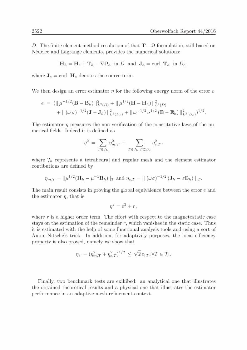
D. The finite element method resolution of that T−Ω formulation, still based onNedelec and Lagrange elements, provides the numerical solutions:
Hh = Hs +Th −∇Ωh in D and Jh = curl Th in Dc ,
where Js = curl Hs denotes the source term.
We then design an error estimator η for the following energy norm of the error e
e = (||µ−1/2(B−Bh) ||2L2(D) + ||µ1/2(H−Hh) ||2L2(D)
+ || (ω σ)−1/2(J− Jh) ||2L2(Dc)+ ||ω−1/2 σ1/2 (E−Eh) ||2L2(Dc)
)1/2.
The estimator η measures the non-verification of the constitutive laws of the nu-merical fields. Indeed it is defined as
η2 =∑
T∈Th
η2m,T +∑
T∈Th,T⊂Dc
η2e,T ,
where Th represents a tetrahedral and regular mesh and the element estimatorcontibutions are defined by
ηm,T = ||µ1/2(Hh − µ−1Bh)||T and ηe,T = || (ωσ)−1/2 (Jh − σEh) ||T .
The main result consists in proving the global equivalence between the error e andthe estimator η, that is
η2 = e2 + r ,
where r is a higher order term. The effort with respect to the magnetostatic casestays on the estimation of the remainder r, which vanishes in the static case. Thusit is estimated with the help of some functional analysis tools and using a sort ofAubin-Nitsche’s trick. In addition, for adaptivity purposes, the local efficiencyproperty is also proved, namely we show that
ηT = (η2m,T + η2e,T )1/2 ≤
√2 e|T , ∀T ∈ Th.
Finally, two benchmark tests are exihibed: an analytical one that illustratesthe obtained theoretical results and a physical one that illustrates the estimatorperformance in an adaptive mesh refinement context.
Adaptive Algorithms 2523
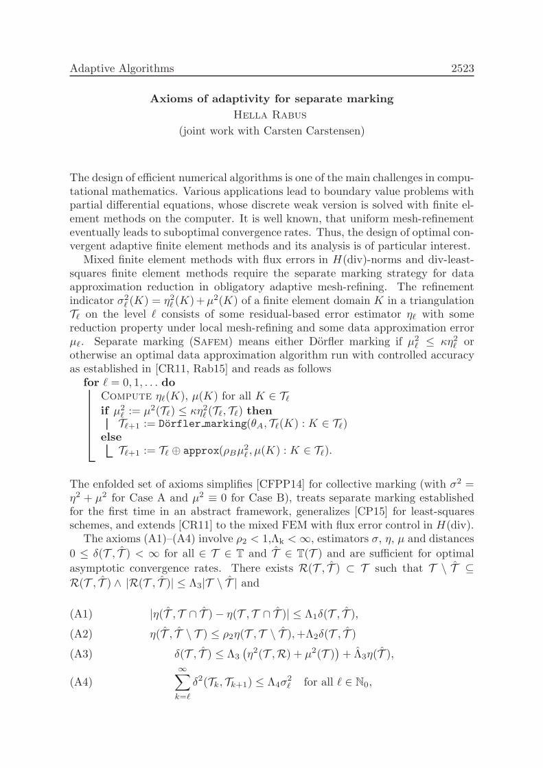
Axioms of adaptivity for separate marking
Hella Rabus
(joint work with Carsten Carstensen)
The design of efficient numerical algorithms is one of the main challenges in compu-tational mathematics. Various applications lead to boundary value problems withpartial differential equations, whose discrete weak version is solved with finite el-ement methods on the computer. It is well known, that uniform mesh-refinementeventually leads to suboptimal convergence rates. Thus, the design of optimal con-vergent adaptive finite element methods and its analysis is of particular interest.
Mixed finite element methods with flux errors in H(div)-norms and div-least-squares finite element methods require the separate marking strategy for dataapproximation reduction in obligatory adaptive mesh-refining. The refinementindicator σ2
ℓ (K) = η2ℓ (K)+µ2(K) of a finite element domain K in a triangulationTℓ on the level ℓ consists of some residual-based error estimator ηℓ with somereduction property under local mesh-refining and some data approximation errorµℓ. Separate marking (Safem) means either Dorfler marking if µ2
ℓ ≤ κη2ℓ orotherwise an optimal data approximation algorithm run with controlled accuracyas established in [CR11, Rab15] and reads as follows
for ℓ = 0, 1, . . . doCompute ηℓ(K), µ(K) for all K ∈ Tℓif µ2
ℓ := µ2(Tℓ) ≤ κη2ℓ (Tℓ, Tℓ) thenTℓ+1 := Dorfler marking(θA, Tℓ(K) : K ∈ Tℓ)
elseTℓ+1 := Tℓ ⊕ approx(ρBµ
2ℓ , µ(K) : K ∈ Tℓ).
The enfolded set of axioms simplifies [CFPP14] for collective marking (with σ2 =η2 + µ2 for Case A and µ2 ≡ 0 for Case B), treats separate marking establishedfor the first time in an abstract framework, generalizes [CP15] for least-squaresschemes, and extends [CR11] to the mixed FEM with flux error control in H(div).
The axioms (A1)–(A4) involve ρ2 < 1,Λk <∞, estimators σ, η, µ and distances
0 ≤ δ(T , T ) < ∞ for all ∈ T ∈ T and T ∈ T(T ) and are sufficient for optimal
asymptotic convergence rates. There exists R(T , T ) ⊂ T such that T \ T ⊆R(T , T ) ∧ |R(T , T )| ≤ Λ3|T \ T | and
|η(T , T ∩ T )− η(T , T ∩ T )| ≤ Λ1δ(T , T ),(A1)
η(T , T \ T ) ≤ ρ2η(T , T \ T ),+Λ2δ(T , T )(A2)
δ(T , T ) ≤ Λ3
(η2(T ,R) + µ2(T )
)+ Λ3η(T ),(A3)
∞∑
k=ℓ
δ2(Tk, Tk+1) ≤ Λ4σ2ℓ for all ℓ ∈ N0,(A4)
2524 Oberwolfach Report 44/2016
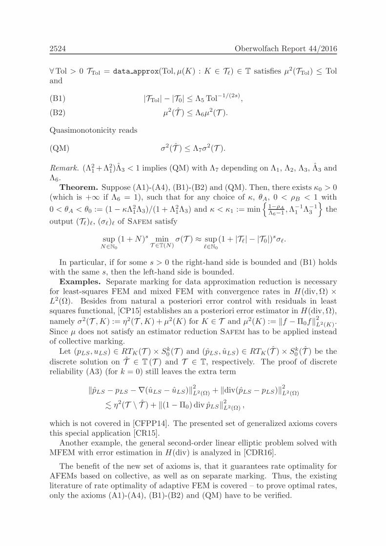
∀Tol > 0 TTol = data approx(Tol, µ(K) : K ∈ Tℓ) ∈ T satisfies µ2(TTol) ≤ Toland
|TTol| − |T0| ≤ Λ5 Tol−1/(2s),(B1)
µ2(T ) ≤ Λ6µ2(T ).(B2)
Quasimonotonicity reads
σ2(T ) ≤ Λ7σ2(T ).(QM)
Remark. (Λ21+Λ2
1)Λ3 < 1 implies (QM) with Λ7 depending on Λ1, Λ2, Λ3, Λ3 andΛ6.
Theorem. Suppose (A1)-(A4), (B1)-(B2) and (QM). Then, there exists κ0 > 0(which is +∞ if Λ6 = 1), such that for any choice of κ, θA, 0 < ρB < 1 with
0 < θA < θ0 := (1 − κΛ21Λ3)/(1 + Λ2
1Λ3) and κ < κ1 := min
1−ρA
Λ6−1 ,Λ−11 Λ−1
3
the
output (Tℓ)ℓ, (σℓ)ℓ of Safem satisfy
supN∈N0
(1 +N)s minT ∈T(N)
σ(T ) ≈ supℓ∈N0
(1 + |Tℓ| − |T0|)sσℓ.
In particular, if for some s > 0 the right-hand side is bounded and (B1) holdswith the same s, then the left-hand side is bounded.
Examples. Separate marking for data approximation reduction is necessaryfor least-squares FEM and mixed FEM with convergence rates in H(div,Ω) ×L2(Ω). Besides from natural a posteriori error control with residuals in leastsquares functional, [CP15] establishes an a posteriori error estimator in H(div,Ω),
namely σ2(T ,K) := η2(T ,K) + µ2(K) for K ∈ T and µ2(K) := ‖f −Π0f‖2L2(K).
Since µ does not satisfy an estimator reduction Safem has to be applied insteadof collective marking.
Let (pLS , uLS) ∈ RTK(T ) × Sk0 (T ) and (pLS , uLS) ∈ RTK(T ) × Sk
0 (T ) be the
discrete solution on T ∈ T (T ) and T ∈ T, respectively. The proof of discretereliability (A3) (for k = 0) still leaves the extra term
‖pLS − pLS −∇(uLS − uLS)‖2L2(Ω) + ‖div(pLS − pLS)‖2L2(Ω)
. η2(T \ T ) + ‖(1−Π0) div pLS‖2L2(Ω) ,
which is not covered in [CFPP14]. The presented set of generalized axioms coversthis special application [CR15].
Another example, the general second-order linear elliptic problem solved withMFEM with error estimation in H(div) is analyzed in [CDR16].
The benefit of the new set of axioms is, that it guarantees rate optimality forAFEMs based on collective, as well as on separate marking. Thus, the existingliterature of rate optimality of adaptive FEM is covered – to prove optimal rates,only the axioms (A1)-(A4), (B1)-(B2) and (QM) have to be verified.
Adaptive Algorithms 2525
References
[CDR16] C. Carstensen, A. Dond, H. Rabus. Quasi-optimality of adaptive mixed FEMs forgeneral second-order linear elliptic problems. in preparation.
[CFPP14] C. Carstensen, M. Feischl, M. Page, and D. Praetorius. Axioms of adaptivity. Comput.Methods Appl. Math., 67(6):1195–1253, 2014.
[CP15] C. Carstensen and E.-J. Park. Convergence and optimality of adaptive least squaresfinite element methods. SIAM J. Numer. Anal., 53:43–62, 2015.
[CR11] C. Carstensen and H. Rabus. An optimal adaptive mixed finite element method. Math.Comp., 80(274):649–667, 2011.
[CR15] C. Carstensen and H. Rabus. Axioms of adaptivity for separate marking.arXiv:1606.02165 [math.NA], 2016.
[Rab15] H. Rabus. Quasi-optimal convergence of AFEM based on separate marking – Part Iand II. Journal of Numerical Analysis, 23(2):137–156, 57–174, 2015.
[Ste08] R. Stevenson. The completion of locally refined simplicial partitions created by bisec-tion. Math. Comp., 77:227–241, 2008.
Adaptive and Multilevel Mixed Finite Element Methods
Jun Hu
This talk consists of three parts. In the first part, we developed a new frameworkto design and analyze the mixed FEM for elasticity problems by establishing thefollowing three main results:
(1) A crucial structure of the discrete stress space: on simplicial grids, the dis-crete stress space can be selected as the symmetric matrix-valued Lagrangeelement space, enriched by a symmetric matrix-valued polynomial H(div)bubble function space on each simplex; a corresponding choice applies toproduct grids.
(2) Two basic algebraic results: (1) on each simplex, the symmetric matrices ofrank one produced by the tensor products of the unit tangent vectors of the(n+1)n/2 edges of the simplex, form a basis of the space of the symmetricmatrices; (2) on each simplex, the divergence space of the above H(div)bubble function space is equal to the orthogonal complement space of therigid motion space with respect to the corresponding discrete displacementspace (Asimilar result holds on a macroelement for the product grids).
These define a two-step stability analysis which is new and different from theclassic one in literature. As a result, on both simplicial and product grids, we wereable to define the first families of both symmetric and optimal mixed elements withpolynomial shape functions in any space dimension. Furthermore, the discretestress space has a simple basis which essentially consists of symmetric matrix-valued Lagrange element basis functions.
On the simplicial grids, in order to avoid enriching H(div,Ω; S)-Pn+1 face-bubble functions of piecewise polynomials or H(div)-Pk nonconforming face-bubble spaces for each n − 1 dimensional simplex for the cases 1 ≤ k ≤ n, wealso designed two classes of stabilized mixed finite element methods. In the firstclass of elements, we use H(div,Ω; S)-Pk and L2(Ω;Rn)-Pk−1 to approximate the

2526 Oberwolfach Report 44/2016
stress and displacement spaces, respectively, for 1 ≤ k ≤ n, and employ a stabi-lization technique in terms of the jump of the discrete displacement over the facesof the triangulation under consideration; in the second class of elements, we useH1
0 (Ω;Rn)-Pk to approximate the displacement space for 1 ≤ k ≤ n, and adopt
the stabilization technique suggested by Brezzi, Fortin, and Marini.In the second part, we developed a block diagonal preconditioner with the min-
imal residual method and a block triangular preconditioner with the generalizedminimal residual method for the aforementioned mixed finite element methods oflinear elasticity. They are based on a new stability result of the saddle point systemin mesh-dependent norms. The mesh-dependent norm for the stress correspondsto the mass matrix which is easy to invert while the displacement it is spectralequivalent to Schur complement. A fast auxiliary space preconditioner based onthe H1 conforming linear element of the linear elasticity problem is then designedfor solving the Schur complement. For both diagonal and triangular precondition-ers, it is proved that the conditioning numbers of the preconditioned systems arebounded above by a constant independent of both the crucial Lame constant andthe mesh-size. Numerical examples are presented to support theoretical results.
In the third part, we studied the convergence and optimality of adaptive mixedfinite element methods (AMFEMs) for the Poisson equations and Stokes equa-tions in an abstract setting. We generalized 6 Hypotheses for the finite elementsubspaces no matter the dimension d = 2 or 3. Under these hypotheses, the con-vergence and optimality can be obtained. As an application, We showed that theRaviart-Thomas elements and the Brezzi-Douglas-Martins elements satisfy thesehypotheses.
References
[1] L. Chen, J. Hu, and X. - H. Huang,Stabilized mixed finite element methods for linearelasticity on simplicial grids in Rn, arXiv:1512.03998, (2015).
[2] L. Chen, J. Hu, and X. - H. Huang, Fast Auxiliary Space Preconditioner for LinearElasticity in Mixed Form, arXiv:1604.02568,2016.
[3] J. Hu, Finite element approximations of symmetric tensors on simplicial grids in Rn: thehigher order case, J. Comput. Math., 33 (2015), pp. 283–296.
[4] J. Hu, A new family of efficient conforming mixed finite elements on both rectangular andcuboid meshes for linear elasticity in the symmetric formulation, SIAM J. Numer. Anal.,53 (2015), pp. 1438–1463.
[5] J. Hu and R. Ma, Conforming mixed triangular prism and nonconforming mixed tetrahedralelements for the linear elasticity problem, arXiv:1604.07903, 2016.
[6] J. Hu, H. Man, and S. Zhang, A simple conforming mixed finite element for linear elas-ticity on rectangular grids in any space dimension, J. Sci. Comput., 58 (2014), pp. 367–379.
[7] J. Hu, H. Man, J. -Y. Wang, and S. Zhang The simplest nonconforming mixed finite
element method for linear elasticity in the symmetric formulation on n-rectangular grids,Comput. Math. Appl., 71(2016), pp. 1317–1336.
[8] J. Hu and Z.-C. Shi, Lower order rectangular nonconforming mixed finite elements forplane elasticity, SIAM J. Numer. Anal., 46 (2007), pp. 88–102.
[9] J. Hu and G.-Z Yu, A unified analysis of quasi-optimal convergence for adaptive mixedfinite element methods, arXiv:1601.00.00132, 2016.
[10] J. Hu and S. Zhang, A family of conforming mixed finite elements for linear elasticity ontriangular grids, arXiv:1406.7457, (2015).

Adaptive Algorithms 2527
[11] J. Hu and S. Zhang, A family of symmetric mixed finite elements for linear elasticity ontetrahedral grids, Sci. China Math., 58 (2015), pp. 297–307.
[12] J. Hu and S. Zhang, Finite element approximations of symmetric tensors on simplicialgrids in Rn: the lower order case, M3AS 26 (2016), pp. 1649–1669.
[13] H.-Y. Man, J. Hu, and Z.-C. Shi, Lower order rectangular nonconforming mixed finiteelement for the three-dimensional elasticity problem, Math. Models Methods Appl. Sci., 19(2009), pp. 51–65.
On Adaptivity in Tree Approximation
Peter Binev
The tree approximation is a convenient way to describe an adaptive approximationinvolving partitioning of a domain in which the next finer partition is formedby subdividing some elements of the current partition into several subsets in aprescribed way. In our considerations we replace ”several” by ”two” mentioningthat this does not restrict the generality since a subdivision into several elementscan be replaced by a sequence of binary subdivisions. The process of the adaptivepartitioning is then described by a full binary tree (a graph in which exactly onenode R, called root, has degree 2 and the other nodes have either degree 1 and arecalled leaves, or degree 3 and are called internal nodes). Naturally, the domainis related to the root R and the current partition is composed by the subsetscorresponding to the leaves L(T ) of the tree T . A subdivision of an element ∆ isperformed by adding two new leaf nodes, ∆′ and ∆′′, to the graph and connectingthem to ∆ which becomes an internal node. We call ∆′ and ∆′′ children of ∆ andrefer to ∆ as their parent. The set A(∆) of ancestors of ∆, including ∆ itself, iscomposed of all nodes on the unique path connecting ∆ with the root R.
A generic adaptive approximation is defined via error functionals e(∆) relatedto the nodes ∆ of a tree T . Each of these functionals represents (an estimate of)the local error of approximation on the subset related to ∆. For example, if weapproximate a function f by piecewise polynomials in Lq, 0 < q < ∞ and P∆ isthe polynomial approximating f on the subset related to ∆, then one can choosee(∆) =
∫∆ |f − P∆|qdx.
We choose no particular form of the error functional but require that it satisfiesthe following subadditivity property:
(1) e(∆) ≥ e(∆′) + e(∆′′) for each node ∆ with children ∆′ and ∆′′ .
It is easy to see that this property is satisfied by (the q-th power of) any integralnorm. However, in the case of local error indicators it should be replaced by itsweak variant discussed in [4]. Here we use (1) for simplicity and to derive resultswith small constants.
The total error of approximation related to a given tree T is defined by E(T ) :=∑∆∈L(T ) e(∆) . The property (1) guarantees that the process of growing the tree T
decreases the error E(T ). To assess how effective this process is, we should compareE(T ) with the smallest possible such error for a tree with similar complexity.
2528 Oberwolfach Report 44/2016
Designating the complexity n := #L(T ) as the number of elements in the partitiongiven by T , we define the best n-term approximation by
σn := minT : #L(T )≤n
E(T ) .
The goal of the adaptive approximation is to design a course-to fine process ofmaking adaptive decisions based only on the information from the errors at thenodes in the current tree. It was proven in [4] that for a particular algorithm, theerror of approximation is compatible to the best one given by σn. Here we presentthe variant of this algorithm provided in [1, 3]. The direct greedy approach, namelysubdividing the leaf ∆ with the largest error e(∆), while being computationallyefficient, does not give an optimal performance. Instead, we define a modifiederror e(∆), setting e(R) := e(R) and then inductively
(2) e(∆) :=e(∆∗) + e(∆)
e(∆∗)e(∆)=
∑
∇∈A(∆)
1
e(∇)
−1
,
where ∆∗ is the parent of ∆. The adaptive algorithm is very simple:
subdivide the leaf ∆ with the largest e(∆).
This type of algorithms are often referred to as h-adaptive since they use the samefixed approximation tool at each node and the improvements come from decreasingof the diameters of the elements of the partition sometimes denoted by h. Thefollowing is the main result about the above algorithm [1, 3].
Theorem 1 Let the tree TN be received by applying a greedy refinement strategywith respect to the quantities e(∆) defined by (2). Then the tree TN provides anear-best h-adaptive approximation
(3) E(TN ) ≤ N
N − n+ 1σn
for any integer n ≤ N . The complexity of the algorithm for obtaining TN is O(N)safe for the sorting of e(∆) that requires O(N logN) operations.
The sorting can be avoided by binning the values of e(∆) into binary bins andchoosing for subdivision any of the ∆ from the largest nonempty bin. This in-creases the constant in (3) by 2 but the total complexity of the algorithm is O(N).
The approximation can be further adapted by varying the number of degrees offreedom p = p(∆) used at each individual element ∆ of the partition. For everyp = 1, 2, ... we consider the corresponding error functional at ∆ denoted by ep(∆).It is reasonable to assume that these errors decrease as p increases, namely
ep(∆) ≥ ep+1(∆) , p ≥ 1 .
In addition, we assume that the subadditivity property (1) also holds but only forthe error functionals e1(∆).
The process of adapting both the partition and the number of degrees of freedomp(∆) at each element ∆ of the partition is known as hp-adaptivity. The approxima-tion is described by the pair (T,P(T )), where P(T ) := p(∇) : ∇ ∈ L(T ) is the
Adaptive Algorithms 2529
list of the assigned degrees of freedom. We define |P(T )| :=∑∇∈L(T ) p(∇) and use
it as a measure of complexity of this approximation. The total error is calculatedas Ehp(T, P (T )) =
∑∇∈L(T ) ep(∇) and the best hp-adaptive approximation is
σhpn := min
Tmin
P(T ) : |P(T )|≤nEhp(T, P (T )) .
An alternative description of the best approximation is using a ”ghost tree” Gwith #L(G) = |P(T )| to distribute the degrees of freedom and for any node ∆ ∈ Gdefines p(∆,G) := #∇ ∈ L(G) : ∆ ∈ A(∇) to match the assignments given byP . In this way, the pair (G, T ) defines an hp-adaptive approximation and it is easyto see that
σhpn = min
G : #L(G)≤nminT⊂G
Ehp(G, T ) .
The following hp-adaptive algorithm describes how to find the ghost tree GN ofcomplexity N = Nmax and the corresponding tree TN :
(1) set G1 := R, T1 := R, e(R) := e(R), E1(R) := e(R), E1(R) := e(∇),q(R) := e(R), s(R) := R, p(R) := 1, and N = 2;
(2) set ∆ := s(R) and expand the current tree GN−1 to GN by subdividing ∆and adding two children nodes ∆′
N and ∆′′N to it;
(3) define TN as the minimal full binary tree containing TN−1, ∆′N , and ∆′′
N ;
(4) for ∇ = ∆′N and ∇ = ∆′′
N calculate the quantities: e(∇) := e(∇)e(∆)e(∇)+e(∆) ,
E1(∇) := e(∇), E1(∇) := e(∇), q(∇) := e(∇), s(∇) := ∇, p(∇) := 1;(5) set p(∆) := p(∆) + 1 and calculate ep(∆)(∆);(6) set ∆′ and ∆′′ to be the children of ∆;(7) set Ep(∆)(∆) := minEp(∆′)(∆
′) + Ep(∆′′)(∆′′) , ep(∆)(∆);
(8) if Ep(∆)(∆) = ep(∆)(∆), then trim T at ∆ making ∆ a leaf node of T ;
(9) set Ep(∆)(∆) :=Ep(∆)(∆)Ep(∆)−1(∆)
Ep(∆)(∆)+Ep(∆)−1(∆);
(10) set D := argmaxq(∆′), q(∆′′) and update
q(∆) := minq(D), Ep(∆)(∆)
, s(∆) := s(D);
(11) if ∆ 6= R, then replace ∆ with its parent and go to (5)(12) else set N := N + 1 and go to (2) or exit if N > Nmax
A near-best performance of the above algorithm is established in [2, 3].
Theorem 2 The pair (GN , TN) provides a near-best hp-adaptive approximation
(4) Ehp(GN , TN) ≤ 2N − 1
N − n+ 1σhpn
for any integer n ≤ N .
The algorithm performs∑
∆∈GNp(∆,GN ) steps, a quantity that varies between
O(N logN) for well balanced trees to O(N2) for highly unbalanced ones. Thiscomplexity can be significantly decreased if ep(∆) changes only at a lacunarysequence of indices p, e.g. at p = 2k setting ep(∆) := e2k(∆) for 2k ≤ p < 2k+1.
2530 Oberwolfach Report 44/2016
This hp-adaptive algorithm was used by Canuto, Nochetto, Stevenson, andVerani in a recent paper [5] to find optimal convergence rates in the univariatecase for a model problem.
References
[1] P. Binev, Adaptive Methods and Near-Best Tree Approximation, Oberwolfach Reports 29(2007), 1669–1673.
[2] P. Binev, Instance optimality for hp-type approximation, Oberwolfach Reports 39 (2013),2192–2194.
[3] P. Binev, Tree approximation for hp-adaptivity, IMI Preprint Series 2015:07[4] P. Binev and R. DeVore, Fast computation in adaptive tree approximation, Numer. Math.
97 (2004), 193–217.[5] C. Canuto, R. H. Nochetto, R. Stevenson, and M. Verani, Convergence and Optimality of
the hp-AFEM, Numer. Math. (2016). doi:10.1007/s00211-016-0826-x
Convergence and Optimality of hp-AFEM
Claudio Canuto
(joint work with Ricardo H. Nochetto, Rob Stevenson, and Marco Verani)
We describe a recently proposed adaptive hp-type finite element algorithm, termedhp-AFEM, for the solution of operator equations such as, e.g., elliptic boundaryvalue problems; the details can be found in [4]. The algorithm produces a se-quence of hp-partitions of the domain (i.e., conforming finite element partitionsequipped with a distribution of polynomial degrees over the elements) and corre-sponding Galerkin discrete solutions, with the following properties: the error inthe energy norm decays at a fixed rate, and is instance optimal, meaning that itis comparable to the best hp-approximation error that can be obtained using acomparable number of degrees of freedom. In particular, if the solution admitshp-type approximations for which the error decays exponentially fast in the num-ber of activated degrees of freedom, the same exponential behavior occurs for theGalerkin approximations built by our algorithm.
A result of this type (exponential convergence through a judicious selection ofh-refinements and p-enrichments) was first obtained by Gui and Babuska [7, 8] forfunctions with localized singularities. However, these pioneering results implicitlyexploit the particular structure of the considered singularities, thus avoiding therisk of making ‘wrong’ choices in the adaptive procedure. Unfortunately, this isnot the generic situation; indeed, it is not difficult to build examples of functions(see again [4] for details) for which early choices between h-refinement and p-enrichment, based on the currently available information, must be subsequentlycorrected in order to stay close to the optimal hp-approximation. In other words,an hp-adaptive algorithm which works for a large class of functions (solutions anddata) should incorporate the possibility of stepping-back, i.e., creating a new hp-partition starting from the available information on the current one, in view ofguaranteeing optimality in the forthcoming steps. This stage is often referred toas ‘coarsening’.
Adaptive Algorithms 2531
Our algorithm hp-AFEM hinges on two routines, termed REDUCE and hp-NEARBEST. The former, starting from the current hp-partition on which dataare already replaced by suitable polynomial approximations (thus in a situationof no ‘data oscillation’) reduces the energy norm of the Galerkin error by a pre-scribed amount. The latter performs the coarsening as indicated above, in orderto guarantee instance optimality of the coarsened approximations; it relies on theadaptive hp-tree approximation routine recently introduced by Binev ([1, 2], seealso his contribution in this Report).
Our algorithm consists of a repetition of calls of hp-NEARBEST and RE-DUCE with decreasing error tolerances. Each call of hp-NEARBEST takes ininput the data and the current Galerkin solution and produces a (nonconforming)hp-partition and a piecewise polynomial approximation of the input functions onthis partition, in such a way that a specific error functional is less than a prescribedtolerance. Such a coarsening procedure, however, may increase the energy normof the Galerkin error by up to a constant factor. This must be compensated by ajudicious choice of the reduction factor of REDUCE so that the concatenation ofthe two routines produces a converging sequence.
The routine REDUCE is implemented as an AFEM consisting of the usual loopover SOLVE, ESTIMATE, MARK, and REFINE. In dimension 1, we construct anestimator that is reliable and discretely efficient, uniformly in p. Consequently, thenumber of iterations to achieve some fixed error reduction is independent on themaximal polynomial degree. In dimension 2, one may employ in ESTIMATE theresidual-based a posteriori error estimator analyzed by Melenk and Wohlmuth [9],which however turns out to be p-sensitive. We show that with this choice, in orderto achieve a fixed error reduction, it suffices to grow the number of iterations morethan quadratically with respect to the maximal polynomial degree. This introducesan optimality degradation at stages intermediate between two consecutive calls ofhp-NEARBEST.
As an alternative, one may resort to the equilibrated flux estimator, whichhas been shown to be p-robust in [3] (see also [6]). We use this estimator tomark stars for refinement, namely patches of elements around vertices, and toexecute p-refinements only. In [5], we provide numerical evidence that a uniformsaturation property holds provided the local polynomial degree p in each markedstar is increased by any quantity proportional to p. Under this choice, the numberof iterations in REFINE needed to reduce the Galerkin error by a fixed amount isuniformly bounded in h and p, thus guaranteeing overall optimality.
References
[1] P. Binev. Instance optimality for hp-type approximation. In Oberwolfach Reports, volume 39,pages 14–16, 2013.
[2] P. Binev. Tree approximation for hp-adaptivity. (in preparation).[3] D. Braess, V. Pillwein, and J. Schoberl. Equilibrated residual error estimates are p-robust.
Comput. Methods Appl. Mech. Engrg., 198(13-14):1189–1197, 2009.[4] C. Canuto, R.H. Nochetto, R. Stevenson, and M. Verani. Convergence and optimality of
hp-AFEM. Numer. Math., 10.1007/s00211-016-0826-x, 2016

2532 Oberwolfach Report 44/2016
[5] C. Canuto, R.H. Nochetto, R. Stevenson, and M. Verani. p-robust saturation property forhp-AFEM, in preparation.
[6] A. Ern and M. Vohralık. Polynomial-degree-robust a posteriori estimates in a unified settingfor conforming, nonconforming, discontinuous Galerkin, and mixed discretizations. SIAMJ. Numer. Anal., 53(2):10581081, 2015.
[7] W. Gui and I. Babuska. The h, p and h-p versions of the finite element method in 1dimension. II. The error analysis of the h- and h-p versions. Numer. Math., 49(6):613–657,1986.
[8] W. Gui and I. Babuska. The h, p and h-p versions of the finite element method in 1dimension. III. The adaptive h-p version. Numer. Math., 49(6):659–683, 1986.
[9] J. M. Melenk and B. I. Wohlmuth. On residual-based a posteriori error estimation in hp-FEM. Adv. Comput. Math., 15(1-4):311–331, 2002.
Robust residual-based a posteriori Arnold-Winther mixed finiteelement analysis in elasticity
Joscha Gedicke
(joint work with Carsten Carstensen)
This talk presents a residual-based a posteriori error estimator for the Arnold-Winther mixed finite element that utilises a post-processing for the skew-symmetricpart of the strain [1]. Numerical experiments verify the proven reliability and ef-ficiency for suitable approximation of the skew-symmetric deformation gradient.Numerical evidence supports that the L2-stress error estimator is robust in thePoisson ratio and allows stable error control even in the incompressible limit.
The problem in linear elasticity considers the connected reference configurationof the elastic body Ω ⊂ R2 with polygonal boundary ∂Ω = ΓD∪ΓN with closed andconnected ΓD of positive surface measure and ΓN = ∂Ω\ΓD for applied tractions.Given a volume force f : Ω → R2, a displacement uD : ΓD → R2, and a tractiong : ΓN → R2, find a displacement u : Ω → R2 and a stress tensor σ : Ω → S :=τ ∈ R2×2 : τ = τT such that
− div σ = f, σ = Cε(u) in Ω,
u = uD on ΓD, σν = g on ΓN ,
where, C denotes the bounded and positive definite fourth-order elasticity tensorfor isotropic linear elasticity.
The a posteriori error analysis for the symmetric Arnold-Winther mixed finiteelement method [2] may follow the ideas of [3] to derive a stress error control
||σ − σAW ||2C−1 ≤ min
v∈V||C−1σAW − ε(uD + v)||2C
+ C1osc2(f, T ) + C2osc
2(g, E(ΓN ))
for the stress error σ−σAW even with a rather explicit estimate of the constant infront of the oscillations and the (unwritten) multiplicative constant 1 in front of thefirst term that measures the quality of the approximation C−1σAW of symmetric
Adaptive Algorithms 2533
gradients ε(v) := (Dv + DT v)/2 for v ∈ V . The space V consists of all square-integrable displacements with homogeneous boundary conditions along ΓD andwith a square-integrable functional matrix Dv.
A severe additional difficulty of this approximation is that only the symmetricpart is approximated and not the full gradient Dv. Other mixed finite elementschemes like PEERS [4] involve some additional variable to approximate the asym-metric part of the gradient. This talk presents an explicit error estimate whichinvolves an arbitrary asymmetric approximation γh and provides an abstract a pos-teriori error control of the residual type, which is useful for adaptive mesh-refiningalgorithms,
η2ℓ = osc2(f, T ) + osc2(g, E(ΓN ))
+∑
T∈T
h2T ‖Curl(C−1σAW + γh)‖2L2(T )
+∑
E∈E(Ω)
hE‖[C−1σAW + γh]τE |2L2(E)
+∑
E∈E(ΓD)
hE‖(C−1σAW + γh −DuD)τ‖2L2(E).
For any (piecewise smooth) choice of γh, this a posteriori error estimator is reliablein the sense that
‖σ − σAW‖C−1 ≤ Crelηℓ
with some λ-independent constant Crel ≈ 1. One opportunity to ensure efficiencyis a global minimisation over all piecewise polynomial γh of the error estimator ηℓ.The bubble function technique shows that the particular choice of γh enters theefficiency estimates with some λ-independent constant Ceff ≈ 1,
ηℓ ≤ Ceff
(‖σ − σAW‖C−1+‖skew(Du)− γh‖L2(Ω)
).
Hence, one efficient choice for γh is to choose it as a sufficiently accurate poly-nomial approximation of the asymmetric gradient skew(Du) := (Du − DTu)/2.Since a global approximation or even minimisation may be too costly, this talkproposes to apply a post-processing step to compute such a sufficiently accurateapproximation γh = skew(Du∗AW ) for the post-processed displacement u∗AW inthe spirit of Stenberg [5]. The approximation γh = skew(Du∗AW ) is proven to berobust in the Poisson ratio ν → 1/2 for sufficiently smooth functions. For domainswith re-entrant corners or incompatible boundary conditions, numerical experi-ments confirm that the proposed computation of γh leads empirically to reliableand efficient a posteriori error control independent of the Poisson ratio ν → 1/2.
References
[1] C. Carstensen and J. Gedicke, Robust residual-based a posteriori Arnold-Winther mixedfinite element analysis in elasticity, Comput. Methods Appl. Mech. Engrg., 300 (2016),245–264.
2534 Oberwolfach Report 44/2016
[2] D. N. Arnold and R. Winther, Mixed finite elements for elasticity, Numer. Math. 92 (2002),401–419.
[3] C. Carstensen and G. Dolzmann, A posteriori error estimates for mixed FEM in elasticity,Numer. Math. 81(2) (1998), 187–209.
[4] D. N. Arnold, F. Brezzi, and J. Douglas, PEERS: A new mixed finite element for planeelasticity, Jpn. J. Appl. Math. 1 (1984), 347–367.
[5] R. Stenberg, A family of mixed finite elements for the elasticity problem, Numer. Math.53(5) (1988), 513–538.
Towards optimal adaptivity of strongly non-symmetric problems
Michael Feischl
Rate optimality of adaptive algorithms has been an active research field since theseminal works [3, 4]. Initially, the research focused on simple symmetric PDEs likethe Poisson equation, but nowadays, many interesting positive definite problemslike (in general non-symmetric) second-order elliptic PDEs, non-local boundaryelement formulations of PDEs, and even certain non-linear problems are under-stood. For a good overview on the known results, we refer to [2]. In stark contrastto this is the development of the theory for strongly non-symmetric problems, i.e.,problems which are more than a compact perturbation of a symmetric equation.The task of proving rate optimality of adaptive algorithms for positive definitenon-symmetric problems is equivalent to proving rate optimality of indefinite sym-metric problems. Hence, the goal of this talk is to understand how non-symmetricor indefinite problems fit into the theory of rate optimality.
1. Rate optimal adaptivity
Let X be a separable Hilbert space of functions on some domain Ω ⊆ Rd. LetT0 denote a triangulation of Ω into compact simplices T ∈ T0. Given a stronglypositive definite and bounded linear operator A : X → X⋆, i.e., 〈Ax , x〉 ≥ c‖x‖2Xfor all x ∈ X , we consider the equation
Ax = f ∈ X⋆.(1)
Moreover, given a refinement (e.g., generated by newest-vertex-bisection) Tℓ of T0,let Xℓ ⊂ X denote the associated finite dimensional subspace of functions (e.g.,piecewise polynomials on Tℓ). We consider the finite-dimensional system: Findxℓ ∈ Xℓ such that
〈Axℓ , y〉 = 〈f , y〉 for all y ∈ Xℓ.(2)
With this, the adaptive algorithm reads:Input: T0. For ℓ = 0, 1, 2, . . . do
a) solve (2),b) compute error estimator to determine elements Mℓ ⊆ Tℓ,c) refine at least the elements in Mℓ to design new triangulation Tℓ+1.

Adaptive Algorithms 2535
By definition, an adaptive algorithm of the above structure is said to be rateoptimal, if the adaptively generated triangulations Tℓ satisfy
err(Tℓ) ≤ C(#Tℓ)−s for all ℓ ∈ N(3)
for all s > 0 which allow for a sequence T optℓ of optimal triangulations (with
T opt0 = T0), generated by the refinement rule of step (c) of the algorithm, such
that err(T optℓ ) ≤ C(#T opt
ℓ )−s. This means that the adaptive algorithm performsat least as good as any other algorithm using the same mesh-refinement. Theerror term err(Tℓ) is usually an upper bound for the error ‖x−xℓ‖X . The work [2]specifies four sufficient (and partly necessary) requirements of the different parts ofthe adaptive algorithm to prove (3). For non-symmetric (or indefinite) problems,the major difficulty appears to be the so called general quasi-orthogonality.
2. General quasi-orthogonality
The most simple form of general quasi-orthogonality reads
∞∑
k=ℓ
‖xk+1 − xk‖2X ≤ C‖x− xℓ‖2X for all ℓ ∈ N.(4)
There exist several generalizations of (4), e.g., for sufficiently small ε ≥ 0
∞∑
k=ℓ
‖xk+1 − xk‖2X − εχ2ℓ ≤ Cerr(Tℓ)2 for all ℓ ∈ N,(5)
where χℓ ∈ err(Tℓ), ‖x− xℓ‖X. This general quasi-orthogonality is the key toolto prove linear convergence of the error in the sense that there exist 0 < q < 1 andC > 0 such that
err(Tℓ+k) ≤ Cqkerr(Tℓ) for all ℓ, k ∈ N.(6)
Furthermore, linear convergence is one of the key tools to prove optimality (3).Moreover, with linear convergence, one can even improve the rate optimality tooptimal complexity in the sense that given some γ > 0, even
err(Tℓ) ≤ C(
ℓ∑
k=0
#T γk )−s for all ℓ ∈ N(7)
holds for all possible s > 0. Since∑ℓ
k=0 #T γk is equivalent to the the overall cost
of the adaptive algorithm (for the right choice of γ, i.e., if each solve-step requiressolving one sparse linear system, we choose γ = 1), this shows that the algorithm isoptimal with respect to computational work. Finally, general quasi-orthogonalityis a direct consequence linear convergence [2, Proposition 4.11], and thus provesto be a central concept of the theory.

2536 Oberwolfach Report 44/2016
3. Towards a proof of general quasi-orthogonality
For symmetric operators A, general quasi-orthogonality (4) follows immediatelyfrom the equivalence ‖ · ‖A := 〈A(·) , (·)〉1/2 ≃ ‖ · ‖X , Galerkin orthogonality
‖xk+1 − xk‖2A = ‖x− xk‖2A − ‖x− xk+1‖2A,(8)
and convergence limℓ→∞ xℓ = x. For strongly non-symmetric (or indefinite) prob-lems, however, (8) does not hold and new ideas are required. The basic approachcan be sketched as follows. Assume that A ∈ RN×N is a lower triangular matrixand let Xℓ = Rℓ ⊂ X := RN . Then, we have xℓ = (A|Rℓ×Rℓ)−1f |Rℓ for all ℓ ∈ N
and hence (up to identification of Rℓ as a subset of RN)
xk+1 − xk = (A|Rk+1×Rk+1)−1f |Rk+1 − (A|Rk×Rk)−1f |Rk = αk+1ek+1,
for the (k + 1)-st unit vector ek+1 ∈ RN and some αk+1 ∈ R. This shows general
quasi-orthogonality (4) by∑N
k=ℓ ‖xk+1 − xk‖2X =∑N
k=ℓ α2k+1 = ‖x− xℓ‖2X .
For a general operator A, the strategy is to find a suitable Riesz basis (wk)k∈N
such that Xℓ := spanw1, . . . , wNℓ for some Nℓ ∈ N and all ℓ ∈ N. Then, the
problems (1)–(2) are equivalent to
Ax = f and A|1,...,Nℓ×1,...,Nℓxℓ = f |1,...,Nℓ,
where A ∈ RN×N, Aij := 〈Awi , wj〉, xℓ ∈ RNℓ , and x,f ∈ RN. The Rieszbasis property guarantees that A : ℓ2 → ℓ2 is a bounded and strongly elliptic
operator. Moreover, there holds xℓ =∑Nℓ
j=1 xℓ,jwj and x =∑∞
j=1 xjwj . Asthe above motivation for the finite dimensional case might suggest, general quasi-orthogonality (4) holds for the original problem (1) if A is sufficiently close to atriangular matrix.
Theorem 1. General quasi-orthogonality (5) holds if A admits a stable (block)LU-factorization, that is, A = LU for matrices L,U ∈ RN×N which are (block)lower resp. upper triangular
(∃ℓ ∈ N, j > Nℓ ≥ i
)=⇒ Lij = Uji = 0
and satisfy that for all ε > 0 there exists Uε ∈ RN×N such that Uε,U−1ε : ℓ2 → ℓ2
are bounded operators and ‖Uε −U‖ℓ2→ℓ∞ ≤ ε.
This theorem leads to several interesting questions.
• When does an infinite matrix posses a stable LU-factorization in the abovesense? Little is known for non-symmetric matrices, see e.g. [1]. Numericalevidence suggests that not every strongly positive definite matrix doeshave a stable LU-factorization. Hence, this class of matrices might be toobig.
• How to characterize the closure L(ℓ2, ℓ2) ⊂ L(ℓ2, ℓ∞)? It is well-knownthat the space of linear operators L(ℓ2, ℓ2) is not dense in L(ℓ2, ℓ∞).
• Can we find a Riesz basis such that A has a simple structure? Wavelettechniques might allow to obtain quasi-sparse matrices A. This can helpto prove the existence of a stable LU-factorization.
Adaptive Algorithms 2537
• What is a general characterization of matrices A which have a stable LU-factorization? This would allow to characterize the class of operatorsA forwhich linear convergence (6) and thus optimal complexity (7) is achievable.
So far, none of the above questions is completely solved. It is the author’sopinion that answering one of those questions can significantly advance the theoryof rate optimality for adaptive algorithms.
References
[1] K. T. Andrews, J. D. Ward, LU-factorization of order bounded operators on Banach se-quence spaces, J. Approx. Theory 48 (1986), 169–180.
[2] C. Carstensen, M. Feischl, M. Page, D. Praetorius, Axioms of adaptivity, Comput. Math.Appl. 67 (2014), 1195–1253.
[3] J. M. Cascon, C. Kreuzer, R. Nochetto, K. G. Siebert, Quasi-optimal convergence rate foran adaptive finite element method, SIAM J. Numer. Anal. 46 (2008), 2524–2550.
[4] R. Stevenson, Optimality of a standard adaptive finite element method, Found. Comput.Math. 7 (2007), 245–269.
Rate optimal adaptive FEM with inexact solverfor strongly monotone operators
Dirk Praetorius
(joint work with Gregor Gantner, Alexander Haberl, and Bernhard Stiftner)
Meanwhile, the mathematical understanding of adaptive FEM has reached a ma-ture state; see [9, 14, 3, 15, 6, 11] for some milestones for linear elliptic PDEs, [17,8, 2, 13] for non-linear problems, and [4] for some general framework. Optimaladaptive FEM with inexact solvers has already been addressed in [15, 1, 4] forlinear PDEs and in [5] for eigenvalue problems. However, for problems involv-ing nonlinear operators, optimal adaptive FEM with inexact solvers has not beenanalyzed yet. Our work [12] aims to close the gap between convergence analysis(e.g. [4]) and empirical evidence (e.g. [10]) by analyzing an algorithm from [7].
Model problem. We follow [4] and present our results from [12] in an abstractframework, while precise examples for our setting are given, e.g., in [2, 13]. Let Hbe a separable Hilbert space over K ∈ R,C with norm ‖ · ‖ and scalar product(·, ·)H. With the duality pairing 〈·, ·〉 between H and its dual H∗, let A : H → H∗
be a nonlinear operator which satisfies the following assumptions:
(O1) A is strongly monotone: There exists α > 0 such that
α ‖u− v‖2 ≤ Re 〈Au −Av, u− v〉 for all u, v ∈ H.(O2) A is Lipschitz continuous: There exists L > 0 such that
‖Au−Av‖∗ := supw∈H\0
〈Au−Av,w〉‖w‖ ≤ L ‖u− v‖ for all u, v ∈ H.
2538 Oberwolfach Report 44/2016
(O3) A has a potential: There exists a Gateaux differentiable function P :H → K with Gateaux derivative dP = A, i.e.,
〈Au, v〉 = limr→0
P (u+ rv)− P (u)
rfor all u, v ∈ H.
Let F ∈ H∗. According to the main theorem on strongly monotone opera-tors [18], (O1)–(O2) imply the existence and uniqueness of u⋆ ∈ H such that
〈Au⋆, v〉 = 〈F, v〉 for all v ∈ H.(1)
To sketch the proof, let I : H → H∗ denote the Riesz mapping defined by 〈Iu, v〉 =(u, v)H for all u, v ∈ H. Then, Φ : H → H, Φ(u) := u− α
L2 I−1(Au− F ) satisfies
‖Φ(u)− Φ(v)‖ ≤ q ‖u− v‖ for all u, v ∈ H, where q := (1− α2/L2)1/2 < 1.(2)
Hence, the Banach fixpoint theorem proves the existence and uniqueness of u⋆ ∈ Hwith Φ(u⋆) = u⋆ which is equivalent to (1). In particular, the Picard iterationun := Φ(un−1) with arbitrary initial guess u0 ∈ H converges to u⋆, and it holds
‖u⋆ − un‖ ≤ q
1− q‖un − un−1‖ ≤ qn
1− q‖u1 − u0‖ for all n ≥ 1.(3)
With (O3), (1) (resp. (4) below) is equivalent to energy minimization, and ‖v−u⋆‖2is equivalent to the energy difference. This guarantees the quasi-orthogonality [4].
FEM with iterative solver based on Picard iteration. Let X• ⊂ H be adiscrete subspace. As in the continuous case, there is a unique u⋆• ∈ X• such that
〈Au⋆•, v•〉 = 〈F, v•〉 for all v• ∈ X•.(4)
According to (O1)–(O2), it holds the Cea-type quasi-optimality ‖u⋆ − u⋆•‖ ≤Lα ‖u⋆ − v•‖ for all v• ∈ X•. To solve the nonlinear system (4), we use the Picard
iteration (applied in X•): Given un−1• ∈ X•, we compute un• = Φ•(u
n−1• ) as follows:
• Solve the linear system (w•, v•)H = 〈Aun−1• − F, v•〉 for all v• ∈ X•.
• Define un• := un−1• − α
L2 w•.
Applying (3) on the discrete level, we infer from [7] that
‖u⋆−un•‖ ≤ ‖u⋆−u⋆•‖+q
1−q ‖un•−un−1
• ‖ ≤ L
αminv•∈X•
‖u⋆−v•‖+qn
1−q ‖u1•−u0•‖.(5)
A posteriori error estimator. We suppose that all considered discrete spacesX• ⊂ H are associated with a conforming triangulation T• of a bounded Lipschitzdomain Ω ⊂ Rd, d ≥ 2. For all T ∈ T• and all v• ∈ X•, we suppose an a posterioricomputable refinement indicator η•(T, v•) ≥ 0. We then define
η•(v•) := η•(T•, v•) and η•(U•, v•)2 :=
∑
T∈U•
η•(T, v•)2 for U• ⊆ T•.(6)
We suppose that there exist constants Cax > 0 and 0 < ax < 1 such that for allT• and all refinements T of T•, the following properties (A1)–(A3) from [4] hold:
(A1) Stability on non-refined element domains:
|η(T• ∩ T, v)− η•(T• ∩ T, v•)| ≤ Cax ‖v − v•‖ for all v• ∈ X•, v ∈ X.

Adaptive Algorithms 2539
(A2) Reduction on refined element domains:
η(T\T•, v) ≤ ax η•(T•\T, v•) + Cax ‖v − v•‖ for all v• ∈ X•, v ∈ X.
(A3) Discrete reliability:
‖u⋆ − u⋆•‖ ≤ Cax η•(T•\T, u⋆•).Note that (A1)–(A2) are required for all discrete functions (and follow from inverseestimates), while (A3) is only required for the discrete solutions u⋆ resp. u⋆• of (4).
Adaptive algorithm. With adaptivity parameters 0 < θ ≤ 1, λ > 0, andCmark ≥ 1, an initial conforming triangulation T0, and an initial guess u00 ∈ X0,our adaptive algorithm iterates the following steps (i)–(iii) for all ℓ = 0, 1, 2, . . .
(i) Repeat (a)–(b) for all n = 1, 2, 3, . . . , until ‖unℓ − un−1ℓ ‖ ≤ λ ηℓ(u
nℓ ).
(a) Compute discrete Picard iterate unℓ ∈ Xℓ.(b) Compute refinement indicators ηℓ(T, u
nℓ ) for all T ∈ Tℓ
(ii) Define uℓ := unℓ and determine a set Mℓ ⊆ Tℓ of minimal cardinality, upto the multiplicative factor Cmark, such that θ ηℓ(uℓ) ≤ ηℓ(Mℓ, uℓ).
(iii) Employ newest vertex bisection [16] to generate the coarsest conformingrefinement Tℓ+1 of Tℓ such that Mℓ ⊆ Tℓ\Tℓ+1 (i.e., all marked elementshave been refined) and define u0ℓ+1 := uℓ ∈ Xℓ ⊆ Xℓ+1.
In step (iii), we suppose that mesh-refinement leads to nested discrete spaces.Lucky break-down of adaptive algorithm. First, if the repeat loop in
step (i) does not terminate, it holds u⋆ ∈ Xℓ. Moreover, there exists C > 0 with
‖u⋆ − unℓ ‖+ ηℓ(unℓ ) ≤ C qn
n→∞−−−−→ 0.(7)
Second, if the repeat loop in step (i) terminates with Mℓ = ∅ in step (ii), thenu⋆ = uk as well as Mk = ∅ for all k ≥ ℓ. Overall, we may thus suppose that therepeat loop in step (i) terminates and that #Tℓ < #Tℓ+1 for all ℓ ≥ 0.
Bounded number of Picard iterations in step (i). There exists C > 0such that nested iteration u0ℓ := uℓ−1 ∈ Xℓ−1 ⊆ Xℓ guarantees
uℓ = unℓ with n ≤ C[1 + log
(max
1,ηℓ−1(uℓ−1)
ηℓ(uℓ)
)]for all ℓ ≥ 1.(8)
Linear convergence. For 0 < θ ≤ 1 and all sufficiently small λ > 0, thereexist constants 0 < < 1 and C > 0 such that
ηℓ+n(uℓ+n) ≤ Cn ηℓ(uℓ) for all ℓ, n ≥ 0.(9)
In particular, there exists C′ > 0 such that
‖u⋆ − uℓ‖ ≤ C′ ηℓ(uℓ) ≤ C′Cℓη0(u0)ℓ→∞−−−→ 0.(10)
Optimal algebraic convergence rates. For sufficiently small 0 < θ ≪ 1,sufficiently small λ > 0, and all s > 0, there exists C > 0 such that
ηℓ(uℓ) ≤ C(#Tℓ −#T0 + 1)−s for all ℓ ≥ 0,(11)
provided that the rate s is possible with respect to certain nonlinear approximationclasses [4, 6].
2540 Oberwolfach Report 44/2016
Optimal computational complexity. Currently, the proof of optimal com-putational complexity is open, but it is observed in numerical experiments.
References
[1] Arioli, Georgoulis, Loghin. SIAM J. Sci. Comput., 35(3):A1537–A1559, 2013.[2] Belenki, Diening, Kreuzer. IMA J. Numer. Anal., 32(2):484–510, 2012.[3] Binev, Dahmen, DeVore. Numer. Math., 97(2):219–268, 2004.[4] Carstensen, Feischl, Page, Praetorius. Comput. Math. Appl., 67(6):1195–1253, 2014.[5] Carstensen, Gedicke. SIAM J. Numer. Anal., 50(3):1029–1057, 2012.[6] Cascon, Kreuzer, Nochetto, Siebert. SIAM J. Numer. Anal., 46(5):2524–2550, 2008.
[7] Congreve, Wihler. J. Comput. Appl. Math., 311:457–472, 2017.[8] Diening, Kreuzer. SIAM J. Numer. Anal., 46(2):614–638, 2008.[9] Dorfler. SIAM J. Numer. Anal., 33(3):1106–1124, 1996.
[10] Ern, Vohralık. SIAM J. Sci. Comput., 35(4):A1761–A1791, 2013.[11] Feischl, Fuhrer, Praetorius. SIAM J. Numer. Anal., 52(2):601–625, 2014.[12] Gantner, Haberl, Praetorius, Stiftner. in preparation, 2016.[13] Garau, Morin, Zuppa. Numer. Math. Theory Methods Appl., 5(2):131–156, 2012.[14] Morin, Nochetto, Siebert. SIAM J. Numer. Anal., 38(2):466–488, 2000.[15] Stevenson. Found. Comput. Math., 7(2):245–269, 2007.[16] Stevenson. Math. Comp., 77(261):227–241, 2008.[17] Veeser. Numer. Math., 92(4):743–770, 2002.[18] Zeidler. Part II/B, Springer, 1990.
Convergence and optimality of adaptive FEM for harmonic forms
Alan Demlow
Harmonic forms arise in computational electromagnetics. More broadly they arean important part of the finite element exterior calculus (FEEC) framework forapproximating solutions to problems of Hodge-Laplace types posed on domainspossibly having nontrivial topology. In the three-dimensional setting, they consistof curl- and divergence-free vector fields satisfying certain boundary conditions.In this talk we prove convergence and rate optimality of adaptive FEM for con-trolling L2 (equivalently, energy) errors in the approximation of harmonic forms.Admissible finite element methods include standard mixed methods based on deRham complex-conforming finite element complexes in all space dimensions.
Proving AFEM convergence results for harmonic forms requires overcoming sev-eral hurdles. The first is non-nestedness, that is, that is, there is no subset relation-ship between spaces of harmonic forms on adjacent mesh levels even if the meshesthemselves are nested. We instead use properties of broader portions of the Hodgedecomposition, resulting in sufficient nestedness and orthogonality properties toobtain AFEM convergence. A second challenge is nonalignment of bases for thespaces of discrete harmonic forms on nested meshes. This is a technical problemthat occurs more generally when approximating multidimensional invariant-typespaces. Typical computational methods do not produced fixed alignments of thebases, so these alignments can change from mesh level to mesh level. We use re-cent techniques developed in the context of eigenvalue AFEM in order to meet thischallenge [1]. Finally, computation of harmonic forms may be either a linear or
Adaptive Algorithms 2541
mildly nonlinear problem, depending on the method used to compute them. Themost general viewpoint, which we take, views the problem as a mildly nonlinearproblem. The result is that some constants in our estimates depend on the degreeof overlap between the space of discrete harmonic forms on the initial mesh andthe (target) space of continuous harmonic forms. We however are able to showthat the dependence of these constants on the initial overlap disappears as themesh is refined.
We finally obtain rate optimality. First we prove a local discrete upper bound.Using essentially standard techniques we then obtain rate optimality using a newargument based on the commuting and locally defined projecting quasi-interpolantof Falk and Winther [2]. As when proving that AFEM contracts, we also discussdependence of various constants on the initial overlap between the continuous anddiscrete spaces of harmonic forms.
References
[1] A. Bonito and A. Demlow, Convergence and optimality of higher-order adaptive finite ele-ment methods for eigenvalue clusters, SIAM J. Numer. Anal. 54 (2016), 2379–2388.
[2] R. Falk and R. Winther Local bounded cochain projections, Math. Comp. 83 (2014), 2631–2656.
Adaptivity and blowup detection for nonlinear parabolic problems
Emmanuil H. Georgoulis
(joint work with Andrea Cangiani, Irene Kyza, Stephen Metcalfe)
In this work, we derive a practical conditional a posteriori bound for a fully-discrete first order in time implicit-explicit (IMEX) interior penalty discontinuousGalerkin (dG) in space discretization of a non self-adjoint semilinear parabolicPDE with quadratic nonlinearity. The choice of an IMEX discretization and,in particular, the explicit treatment of the nonlinearity, offers advantages in thecontext of finite time blow-up – this is highlighted below via the discretization ofthe related ODE problem with various time-stepping schemes. The choice of a dGmethod in space offers stability of the spatial operator in convection-dominatedregimes on coarse meshes; we stress, however, that the theory presented belowis directly applicable to the case of conforming finite element approximations inspace. The conditional a posteriori error bounds are derived in the L∞(L2) +L2(H1)-type norm. The derivation is based on energy techniques combined withthe Gagliardo-Nirenberg inequality while retaining the key idea introduced in [6]– judicious usage of Gronwall’s lemma. A key novelty of our approach is theuse of a local-in-time continuation argument in conjunction with a space-timereconstruction. Global-in-time continuation arguments have been used to deriveconditional a posteriori error estimates for finite element discretizations of PDEswith globally bounded solutions, cf. [1, 4, 5]. A useful by-product of the localcontinuation argument used in this work is that it gives a natural stopping criterionfor approach towards the blow-up time. The use of space-time reconstruction,

2542 Oberwolfach Report 44/2016
introduced in [7, 8] for conforming finite element methods and in [2, 3] for dGmethods, allows for the derivation of a posteriori bounds in norms weaker thanL2(H1) and offers great flexibility in treating general spatial operators and theirrespective discretizations.
Furthermore, a space-time adaptive algorithm is proposed which uses the con-ditional a posteriori bound to control the time step lengths and the spatial meshmodifications. The adaptive algorithm is a non-trivial modification of typicaladaptive error control procedures for parabolic problems. In the proposed adap-tive algorithm, the tolerances are adapted in the run up to blow-up time to allowfor larger absolute error in an effort to balance the relative error of the approxima-tion. The space-time adaptive algorithm is tested on three numerical experiments,two of which exhibit point blow-up and one which exhibits regional blow-up. Eachtime the algorithm appears to detect and converge to the blow-up time withoutsurpassing it.
References
[1] S. Bartels, A posteriori error analysis for time-dependent Ginzburg-Landau type equations,Numer. Math., 99 (2005), pp. 557–583.
[2] A. Cangiani, E. H. Georgoulis, and S. Metcalfe, Adaptive discontinuous Galerkinmethods for nonstationary convection-diffusion problems, IMA J. Numer. Anal., 34 (2014),pp. 1578–1597.
[3] E. H. Georgoulis, O. Lakkis, and J. M. Virtanen, A posteriori error control for dis-continuous Galerkin methods for parabolic problems, SIAM J. Numer. Anal., 49 (2011),pp. 427–458.
[4] E. H. Georgoulis and C. Makridakis, On a posteriori error control for the Allen-Cahnproblem, Math. Method. Appl. Sci., 37 (2014), pp. 173–179.
[5] D. Kessler, R. H. Nochetto, and A. Schmidt, A posteriori error control for the Allen-Cahn problem: circumventing Gronwall’s inequality, ESAIM Math. Model. Numer. Anal.,38 (2004), pp. 129–142.
[6] I. Kyza and C. Makridakis, Analysis for time discrete approximations of blow-up solutionsof semilinear parabolic equations, SIAM J. Numer. Anal., 49 (2011), pp. 405–426.
[7] O. Lakkis and C. Makridakis, Elliptic reconstruction and a posteriori error estimates forfully discrete linear parabolic problems, Math. Comp., 75 (2006), pp. 1627–1658.
[8] C. Makridakis and R. H. Nochetto, Elliptic reconstruction and a posteriori error esti-mates for parabolic problems, SIAM J. Numer. Anal., 41 (2003), pp. 1585–1594.
Linearization of the p-Poisson equation
Lars Diening
(joint work with M. Wank, M. Fornasier, R. Tomasi)
The p-Poisson problem consists in finding the solution u ∈W 1,p0 (Ω) of
− div(|∇u|p−2∇u
)= f
for 1 < p <∞ and suitable f . The function umay be scalar or vectorial. For p = 2this is the standard Poisson problem, but for p 6= 2 the problem is non-linear.
Our goal is to approximate the solution by means of the finite element method.Many results have appeared in this direction. The a priori analysis goes back to
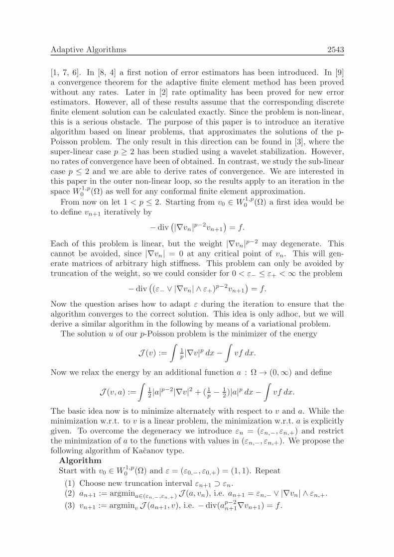
Adaptive Algorithms 2543
[1, 7, 6]. In [8, 4] a first notion of error estimators has been introduced. In [9]a convergence theorem for the adaptive finite element method has been provedwithout any rates. Later in [2] rate optimality has been proved for new errorestimators. However, all of these results assume that the corresponding discretefinite element solution can be calculated exactly. Since the problem is non-linear,this is a serious obstacle. The purpose of this paper is to introduce an iterativealgorithm based on linear problems, that approximates the solutions of the p-Poisson problem. The only result in this direction can be found in [3], where thesuper-linear case p ≥ 2 has been studied using a wavelet stabilization. However,no rates of convergence have been of obtained. In contrast, we study the sub-linearcase p ≤ 2 and we are able to derive rates of convergence. We are interested inthis paper in the outer non-linear loop, so the results apply to an iteration in thespace W 1,p
0 (Ω) as well for any conformal finite element approximation.
From now on let 1 < p ≤ 2. Starting from v0 ∈ W 1,p0 (Ω) a first idea would be
to define vn+1 iteratively by
− div(|∇vn|p−2vn+1
)= f.
Each of this problem is linear, but the weight |∇vn|p−2 may degenerate. Thiscannot be avoided, since |∇vn| = 0 at any critical point of vn. This will gen-erate matrices of arbitrary high stiffness. This problem can only be avoided bytruncation of the weight, so we could consider for 0 < ε− ≤ ε+ <∞ the problem
− div((ε− ∨ |∇vn| ∧ ε+)p−2vn+1
)= f.
Now the question arises how to adapt ε during the iteration to ensure that thealgorithm converges to the correct solution. This idea is only adhoc, but we willderive a similar algorithm in the following by means of a variational problem.
The solution u of our p-Poisson problem is the minimizer of the energy
J (v) :=
∫1p |∇v|p dx−
∫vf dx.
Now we relax the energy by an additional function a : Ω → (0,∞) and define
J (v, a) :=
∫12 |a|p−2|∇v|2 + ( 1p − 1
2 )|a|p dx−∫vf dx.
The basic idea now is to minimize alternately with respect to v and a. While theminimization w.r.t. to v is a linear problem, the minimization w.r.t. a is explicitlygiven. To overcome the degeneracy we introduce εn = (εn,−, εn,+) and restrictthe minimization of a to the functions with values in (εn,−, εn,+). We propose thefollowing algorithm of Kacanov type.AlgorithmStart with v0 ∈W 1,p
0 (Ω) and ε = (ε0,−, ε0,+) = (1, 1). Repeat
(1) Choose new truncation interval εn+1 ⊃ εn.(2) an+1 := argmina∈(εn,−,εn,+) J (a, vn), i.e. an+1 = εn,− ∨ |∇vn| ∧ εn,+.(3) vn+1 := argminv J (an+1, v), i.e. − div(ap−2
n+1∇vn+1) = f .
2544 Oberwolfach Report 44/2016
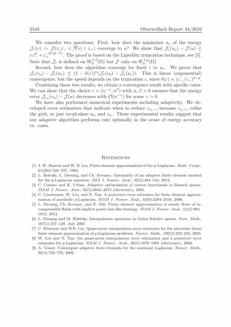
We consider two questions: First, how does the minimizer uε of the energyJε(v) := J (v, ε− ∨ |∇v| ∧ ε+) converge to u? We show that Jε(uε) − J (u) ≤c εp−+ε
−d/(p−1)+ . The proof is based on the Lipschitz truncation technique, see [5].
Note that Jε is defined on W 1,20 (Ω) but J only on W 1,p
0 (Ω).Second, how does the algorithm converge for fixed ε to uε. We prove that
Jε(vn) − Jε(uε) ≤ (1 − δ(ε))n(Jε(v0) − Jε(uε)). This is linear (exponential)convergence, but the speed depends on the truncation ε, since δ(ε) h (ε−/ε+)
2−p.Combining these two results, we obtain a convergence result with specific rates.
We can show that the choice ε = (n−α, nβ) with α, β > 0 ensures that the energyerror Jεn(vn)− J (u) decreases with O(n−γ) for some γ > 0.
We have also performed numerical experiments including adaptivity. We de-veloped error estimators that indicate when to reduce εn,−, increase εn,+, refinethe grid, or just recalculate an and vn. These experimental results suggest thatour adaptive algorithm performs rate optimally in the sense of energy accuracyvs. costs.
References
[1] J. W. Barrett and W. B. Liu. Finite element approximation of the p-Laplacian.Math. Comp.,61(204):523–537, 1993.
[2] L. Belenki, L. Diening, and Ch. Kreuzer. Optimality of an adaptive finite element methodfor the p-Laplacian equation. IMA J. Numer. Anal., 32(2):484–510, 2012.
[3] C. Canuto and K. Urban. Adaptive optimization of convex functionals in Banach spaces.SIAM J. Numer. Anal., 42(5):2043–2075 (electronic), 2005.
[4] C. Carstensen, W. Liu, and N. Yan. A posteriori error estimates for finite element approxi-mation of parabolic p-Laplacian. SIAM J. Numer. Anal., 43(6):2294–2319, 2006.
[5] L. Diening, Ch. Kreuzer, and E. Suli. Finite element approximation of steady flows of in-compressible fluids with implicit power-law-like rheology. SIAM J. Numer. Anal., 51(2):984–1015, 2013.
[6] L. Diening and M. Ruzicka. Interpolation operators in Orlicz Sobolev spaces. Num. Math.,
107(1):107–129, July 2007.[7] C. Ebmeyer and WB. Liu. Quasi-norm interpolation error estimates for the piecewise linear
finite element approximation of p-Laplacian problems. Numer. Math., 100(2):233–258, 2005.[8] W. Liu and N. Yan. On quasi-norm interpolation error estimation and a posteriori error
estimates for p-Laplacian. SIAM J. Numer. Anal., 40(5):1870–1895 (electronic), 2002.[9] A. Veeser. Convergent adaptive finite elements for the nonlinear Laplacian. Numer. Math.,
92(4):743–770, 2002.
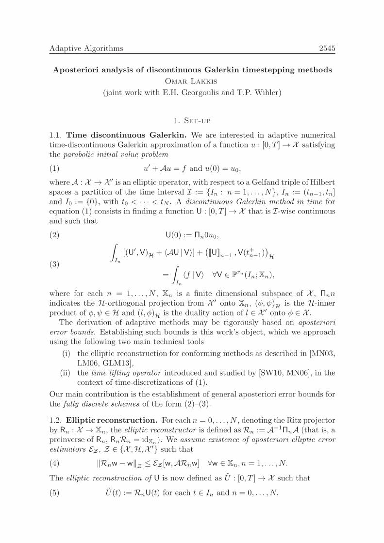
Adaptive Algorithms 2545
Aposteriori analysis of discontinuous Galerkin timestepping methods
Omar Lakkis
(joint work with E.H. Georgoulis and T.P. Wihler)
1. Set-up
1.1. Time discontinuous Galerkin. We are interested in adaptive numericaltime-discontinuous Galerkin approximation of a function u : [0, T ] → X satisfyingthe parabolic initial value problem
(1) u′ +Au = f and u(0) = u0,
whereA : X → X ′ is an elliptic operator, with respect to a Gelfand triple of Hilbertspaces a partition of the time interval I := In : n = 1, . . . , N, In := (tn−1, tn]and I0 := 0, with t0 < · · · < tN . A discontinuous Galerkin method in time forequation (1) consists in finding a function U : [0, T ] → X that is I-wise continuousand such that
U(0) := Πn0u0,(2)∫
In
[(U′,V)H + 〈AU |V〉] +([[U]]n−1 ,V(t
+n−1)
)H
=
∫
In
〈f |V〉 ∀V ∈ Prn(In;Xn),
(3)
where for each n = 1, . . . , N , Xn is a finite dimensional subspace of X , Πnnindicates the H-orthogonal projection from X ′ onto Xn, (φ, ψ)H is the H-innerproduct of φ, ψ ∈ H and (l, φ)H is the duality action of l ∈ X ′ onto φ ∈ X .
The derivation of adaptive methods may be rigorously based on aposteriorierror bounds. Establishing such bounds is this work’s object, which we approachusing the following two main technical tools
(i) the elliptic reconstruction for conforming methods as described in [MN03,LM06, GLM13],
(ii) the time lifting operator introduced and studied by [SW10, MN06], in thecontext of time-discretizations of (1).
Our main contribution is the establishment of general aposteriori error bounds forthe fully discrete schemes of the form (2)–(3).
1.2. Elliptic reconstruction. For each n = 0, . . . , N , denoting the Ritz projectorby Rn : X → Xn, the elliptic reconstructor is defined as Rn := A−1
ΠnA (that is, apreinverse of Rn, RnRn = idXn). We assume existence of aposteriori elliptic errorestimators EZ , Z ∈ X ,H,X ′ such that
(4) ‖Rnw− w‖Z ≤ EZ [w,ARnw] ∀w ∈ Xn, n = 1, . . . , N.
The elliptic reconstruction of U is now defined as U : [0, T ] → X such that
(5) U(t) := RnU(t) for each t ∈ In and n = 0, . . . , N.
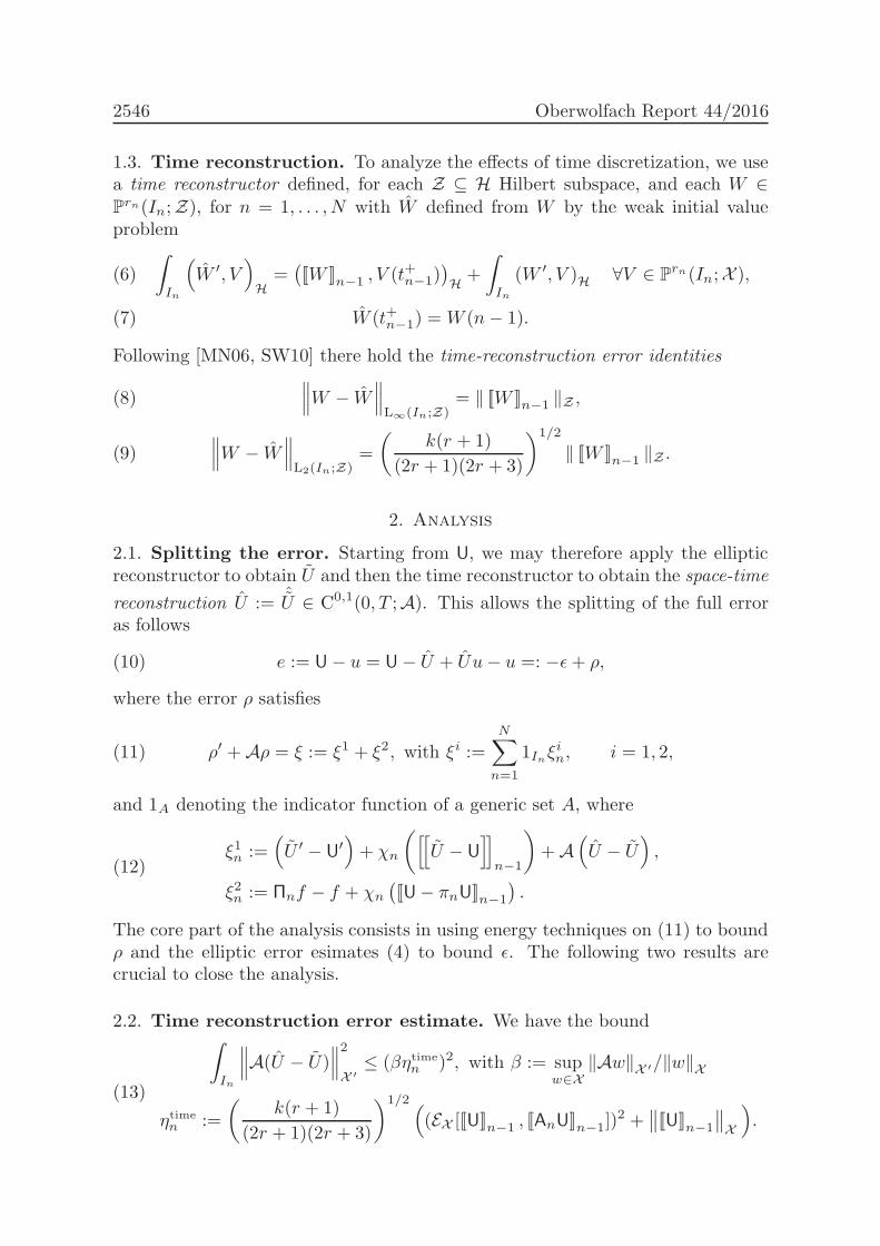
2546 Oberwolfach Report 44/2016
1.3. Time reconstruction. To analyze the effects of time discretization, we usea time reconstructor defined, for each Z ⊆ H Hilbert subspace, and each W ∈Prn(In;Z), for n = 1, . . . , N with W defined from W by the weak initial valueproblem
∫
In
(W ′, V
)H
=([[W ]]n−1 , V (t+n−1)
)H+
∫
In
(W ′, V )H ∀V ∈ Prn(In;X ),(6)
W (t+n−1) =W (n− 1).(7)
Following [MN06, SW10] there hold the time-reconstruction error identities∥∥∥W − W
∥∥∥L∞(In;Z)
= ‖ [[W ]]n−1 ‖Z ,(8)
∥∥∥W − W∥∥∥L2(In;Z)
=
(k(r + 1)
(2r + 1)(2r + 3)
)1/2
‖ [[W ]]n−1 ‖Z .(9)
2. Analysis
2.1. Splitting the error. Starting from U, we may therefore apply the ellipticreconstructor to obtain U and then the time reconstructor to obtain the space-time
reconstruction U := ˆU ∈ C0,1(0, T ;A). This allows the splitting of the full erroras follows
(10) e := U− u = U− U + Uu− u =: −ǫ+ ρ,
where the error ρ satisfies
(11) ρ′ +Aρ = ξ := ξ1 + ξ2, with ξi :=
N∑
n=1
1Inξin, i = 1, 2,
and 1A denoting the indicator function of a generic set A, where
(12)ξ1n :=
(U ′ − U
′)+ χn
([[U − U
]]n−1
)+A
(U − U
),
ξ2n := Πnf − f + χn
([[U− πnU]]n−1
).
The core part of the analysis consists in using energy techniques on (11) to boundρ and the elliptic error esimates (4) to bound ǫ. The following two results arecrucial to close the analysis.
2.2. Time reconstruction error estimate. We have the bound
(13)
∫
In
∥∥∥A(U − U)∥∥∥2
X ′
≤ (βηtimen )2, with β := sup
w∈X‖Aw‖X ′/‖w‖X
ηtimen :=
(k(r + 1)
(2r + 1)(2r + 3)
)1/2 ((EX [[[U]]n−1 , [[AnU]]n−1])
2 +∥∥[[U]]n−1
∥∥X
).
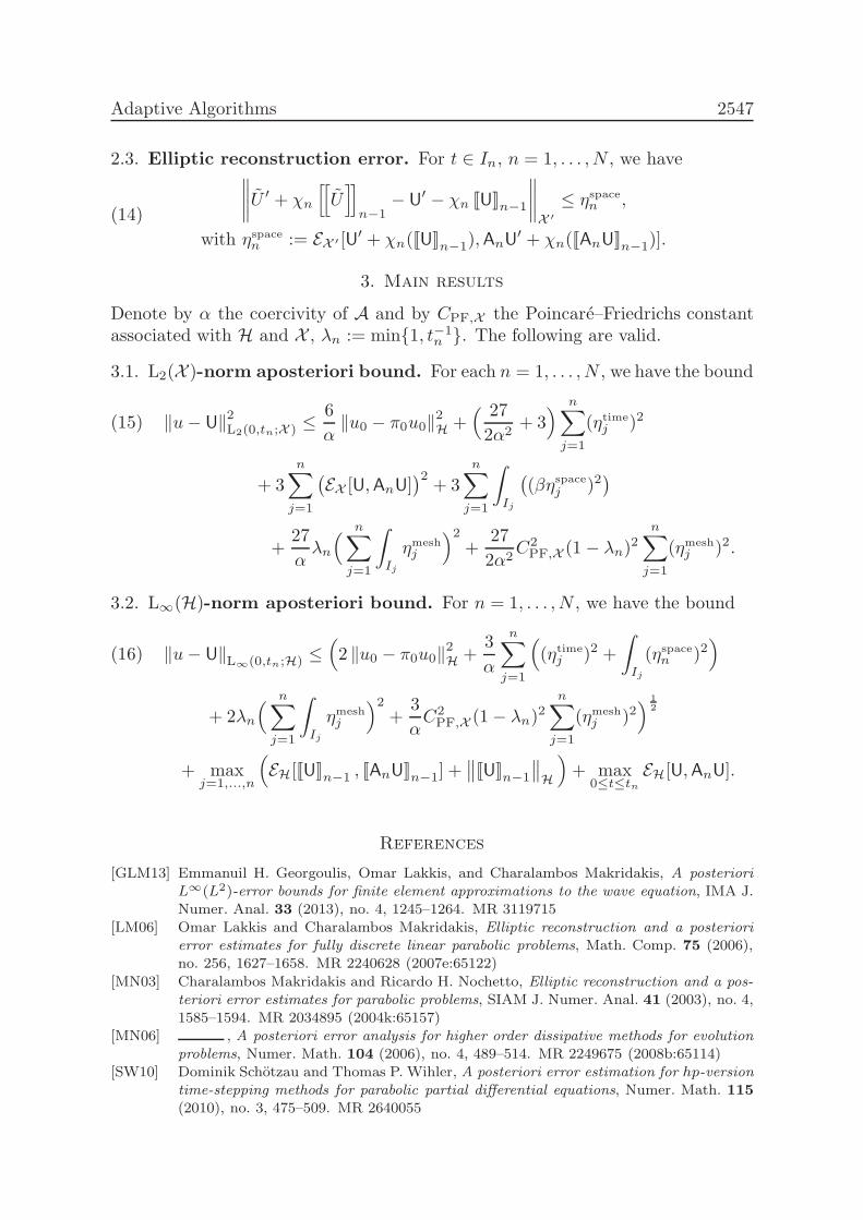
Adaptive Algorithms 2547
2.3. Elliptic reconstruction error. For t ∈ In, n = 1, . . . , N , we have
(14)
∥∥∥∥U′ + χn
[[U]]
n−1− U
′ − χn [[U]]n−1
∥∥∥∥X ′
≤ ηspacen ,
with ηspacen := EX ′ [U′ + χn([[U]]n−1),AnU′ + χn([[AnU]]n−1)].
3. Main results
Denote by α the coercivity of A and by CPF,X the Poincare–Friedrichs constantassociated with H and X , λn := min1, t−1
n . The following are valid.
3.1. L2(X )-norm aposteriori bound. For each n = 1, . . . , N , we have the bound
(15) ‖u− U‖2L2(0,tn;X ) ≤6
α‖u0 − π0u0‖2H +
( 27
2α2+ 3) n∑
j=1
(ηtimej )2
+ 3
n∑
j=1
(EX [U,AnU]
)2+ 3
n∑
j=1
∫
Ij
((βηspacej )2
)
+27
αλn
( n∑
j=1
∫
Ij
ηmeshj
)2+
27
2α2C2
PF,X (1 − λn)2
n∑
j=1
(ηmeshj )2.
3.2. L∞(H)-norm aposteriori bound. For n = 1, . . . , N , we have the bound
(16) ‖u− U‖L∞(0,tn;H) ≤(2 ‖u0 − π0u0‖2H +
3
α
n∑
j=1
((ηtime
j )2 +
∫
Ij
(ηspacen )2)
+ 2λn
( n∑
j=1
∫
Ij
ηmeshj
)2+
3
αC2
PF,X (1− λn)2
n∑
j=1
(ηmeshj )2
) 12
+ maxj=1,...,n
(EH[[[U]]n−1 , [[AnU]]n−1] +
∥∥[[U]]n−1
∥∥H
)+ max
0≤t≤tnEH[U,AnU].
References
[GLM13] Emmanuil H. Georgoulis, Omar Lakkis, and Charalambos Makridakis, A posterioriL∞(L2)-error bounds for finite element approximations to the wave equation, IMA J.Numer. Anal. 33 (2013), no. 4, 1245–1264. MR 3119715
[LM06] Omar Lakkis and Charalambos Makridakis, Elliptic reconstruction and a posteriorierror estimates for fully discrete linear parabolic problems, Math. Comp. 75 (2006),no. 256, 1627–1658. MR 2240628 (2007e:65122)
[MN03] Charalambos Makridakis and Ricardo H. Nochetto, Elliptic reconstruction and a pos-teriori error estimates for parabolic problems, SIAM J. Numer. Anal. 41 (2003), no. 4,1585–1594. MR 2034895 (2004k:65157)
[MN06] , A posteriori error analysis for higher order dissipative methods for evolutionproblems, Numer. Math. 104 (2006), no. 4, 489–514. MR 2249675 (2008b:65114)
[SW10] Dominik Schotzau and Thomas P. Wihler, A posteriori error estimation for hp-versiontime-stepping methods for parabolic partial differential equations, Numer. Math. 115(2010), no. 3, 475–509. MR 2640055

2548 Oberwolfach Report 44/2016
Adaptive sparse and low-rank methods for parametric PDEs
Wolfgang Dahmen
(joint work with Markus Bachmayr, Albert Cohen)
Parameter dependent families of partial differential equations (PDEs) arise in adiversity of contexts. For instance, Karhunen-Loeve, polynomial chaos or othertypes of expansions of random coefficient fields in a PDE, in principle, give riseto even infinitely many parameters. Therefore, we consider a class of parametricoperator equations where the involved parameters could either be of deterministicor stochastic nature. Specifically, we focus on scenarios involving a large numberof parameters in the context of elliptic boundary value problems of the type
(1) −div(a(y)∇u) = f in Ω, u = 0 on ∂Ω, y ∈ Y := [−1, 1]I,
where the coefficient field is given as an expansion
(2) a(x, y) = a0(x) +∑
j∈I
yjθj(x)
subject to suitable conditions on the θj that ensure convergence of the expansionas well as uniform ellipticity of the operator. Thus, (1) has a unique solution(as a function of the spatial variables x as well as of the parametric variablesy ∈ Y = [−1, 1]I) in L2(Y, H1
0 (Ω)) = H10 (Ω) ⊗ L2(Y). As mentioned before,
#(I) = ∞ is permitted in which case u(y) = u(·, y) can be understood as thelimit of solutions to finitely parametrized problems obtained by truncating theexpansion (2). Hence, in this case the anisotropy of the parameter dependence,induced by the decay conditions on the expansion (2), is essential.
From a practical point of view a typical “forward” simulation task concernsthe approximate computation of a quantity of interest such as the expectationof the solution in the stochastic case or local spatial averages as functions of theparameters. In either case one is confronted in one way or the other with whatis commonly referred to as “curse of dimensionality”. Therefore, understandingthe whole parameter-to-solution map y 7→ u(y) is of fundamental importance, seee.g. [6, 7, 11] and the references therein. On the theoretical side the vast majorityof contributions to this problem area are concerned with sparse polynomial para-metric expansions. One such strategy is based on performing sparse best n-termapproximations of the solution map in an a priori chosen system of tensor productform in the parametric variables. This approach has been extensively analyzed inthe case of tensor product Legendre polynomial bases, for which approximationrates have been established, see e.g. [3, 3]. On the practical side, a prominent ap-proach is to combine such expansions with collocation, see e.g. [4]. The complexityanalysis of such methods is essentially based on a priori estimates.
An alternative strategy for addressing the challenges posed by high dimension-ality is to use low-rank approximations of solutions based on a separation of spatialand parametric variables. In this respect we review here some recent results from[2] which, in particular, ask what can be gained by exploiting further low rankstructures, in particular using optimized systems of basis functions obtained by

Adaptive Algorithms 2549
singular value decomposition techniques. Based on the concepts from [1], a genericadaptive solver is proposed that is guaranteed to achieve a given target accuracyafter finitely many steps without requiring any a priori knowledge about the solu-tion. Moreover, it can be specified so as to produce approximate solutions to (1)in each of the following approximation formats: (a) sparse n-term approximationwith respect a fixed background basis for H1
0 (Ω)⊗L2(Y), (b) Hilbert-Schmidt typelow-rank approximations separating spatial and parametric variables, as well as (c)approximate solutions in hierarchical tensor formats separating also all paramet-ric variables. The latter variant is suited best for a possibly large but fixed finitenumber of parametric variables with “equal importance“. Although it involvesa similar format as [10] it is conceptually different and can be shown to exhibitnear-optimal performance with respect to relevant approximation classes, see [2].Therefore, we confine the subsequent discussion to the two former variants (a), (b)focusing on the case of ininitely many parameters of “anisotropic importance”, re-marking that for variant (a) the scheme agrees in essence with the one proposedin [5] in the wavelet context and extended to parametric PDEs in [12, 13].
On the theoretical side, inspired by the findings in [3], several model scenariosare presented which show that optimized low-rank expansions can either bringsignificant or no improvement over sparse polynomial expansions, regarding thenumber of terms needed to realize a given target accuracy. On the computationalside, the complexity of the adaptive solver is analyzed for its respective specifica-tion to (b) low-rank structure as well as (a) sparse background basis expansions.First, guided by the above mentioned model scenarios, benchmark classes areintroduced which quantifiy the expceted approximability properties of solutionswith respect to the decay of singular values, sparsity of the (lower-dimensional)Hilbert-Schmidt factors, or of expansions in terms of the fixed background basisfor H1
0 (Ω) ⊗ L2(Y). Moreover, it is indicated that specific types of parametricexpansions (2) have a significant effect on the performance on algorithms based ona posteriori residual evaluations. Specifically, in contrast to Karhunen-Loeve typerepresentations, expansion functions θj of multilevel or wavelet type allow one tofully exploit the approximability properties given in the benchmark classes. Infact, the algorithm is shown to realize then near-best convergence and complexityrates for both variants (a) and (b) improving somewhat on the results in [13] withregard to (a). Adaptive solvers based on finite element discretizations in the spa-tial variable have been proposed also in [8, 9] where, however, the complexity withrespect to the parametric components does not seem to be controled. An essentialdifference between the algorithm discussed here from those in [10, 8, 9] lies in: (i) anew adaptive operator application scheme using a posteriori information througha judicious decomposition of the current aproximation and a careful compressibil-ity analysis of the operator components; (ii) threshold based tensor-recompressionand coarsening schemes in the spirit of [5, 1]. Some numerical experiments quan-tify the theoretical findings and support the predictions derived from the above
2550 Oberwolfach Report 44/2016
mentioned model scenarios. On the other hand, the price for the obtained near-optimal performance is a high level of intrusiveness, i.e., standard numerical toolscannot easily be incorporated.
References
[1] M. Bachmayr, W. Dahmen, Adaptive near-optimal rank tensor approximation for high-dimensional operator equations, Found. Comput. Math., 15 (No. 4) (2015), 839–898, DOI10.1007/s10208-013-9187-3.
[2] M. Bachmayr, A. Cohen, W. Dahmen, Parametric PDEs: Sparse or low-rank approxima-tions? July 2016, http://arxiv.org/abs/1607.04444 [math.NA].
[3] M. Bachmayr, A. Cohen, G. Migliorati, Sparse polynomial approximation of parametricelliptic PDEs. Part I: affine coefficients, 2015, arXiv:1509.07045 [math.NA],
[4] J. Beck, R. Tempone, F. Nobile, L. Tamellini, On the optimal polynomial approximation ofstochastic PDEs by Galerkin and collocation methods, Math. Models Methods Appl. Sci.,22 (No.9), (2012), DOI 10.1142/S0218202512500236,
[5] A. Cohen, W. Dahmen, R. DeVore, Adaptive wavelet methods II – beyond the elliptic case,Foundations of Computational Mathematics, 2 (No. 3) (2002), 203–245.
[6] A. Cohen, R. DeVore, Approximation of high-dimensional parametric PDEs, Acta Numer.,24, (2015), 1–159, DOI 10.1017/S0962492915000033.
[7] A. Cohen, R. DeVore, Ch. Schwab, Convergence rates of best N-term Galerkin approxima-tions for a class of elliptic sPDEs, Found. Comput. Math., 10, (No.6) (2010), 615–646, DOI10.1007/s10208-010-9072-2.
[8] M. Eigel,C.J. Gittelson, Ch. Schwab, E. Zander, Adaptive stochastic Galerkin FEM, Com-put. Methods Appl. Mech. Engrg., 270 (2014), 247–269, DOI10.1016/j.cma.2013.11.015.
[9] M. Eigel, C.J. Gittelson, Ch. Schwab, E. Zander, A convergent adaptive stochastic Galerkinfinite element method with quasi-optimal spatial meshes, ESAIM: M2AN, 49, (No.5) (2015),1367–1398.
[10] M. Eigel,M. Pfeffer, R. Schneider, Adaptive stochastic Galerkin FEM with hierarchical ten-sor representions, Preprint 2153, 2015, WIAS Berlin,
[11] C.J. Gittelson, Ch. Schwab, Sparse tensor discretization of high-dimensional parametricand stochastic PDEs, Acta Numerica, 20 (2011),
[12] C.J. Gittelson, An adaptive stochastic Galerkin method for random elliptic operators, Math-ematics of Computation, 82 (2013), 1515–1541.
[13] C.J. Gittelson, Adaptive wavelet methods for elliptic partial differential equations with ran-dom operators, Numer. Math., 126 (2014), 471–513.
On the discrete reliability for nonconforming finite element methods
Dietmar Gallistl
(joint work with Carsten Carstensen, Mira Schedensack)
Let T be a simplicial partition of the bounded Lipschitz polytope Ω ⊆ Rn, n ≥ 2.Classical a posteriori error estimates for finite element discretizations of ellipticpartial differential equations (PDEs) posed in the Sobolev space H1
0 (Ω) (for in-stance Poisson’s equation) usually take the form
‖∇(u− uT )‖2L2(Ω) ≤ Crel
∑
T∈T
η2T (uT )
where u is the solution to the PDE and uT is its finite element approximation withrespect to the mesh T . The bound on the right hand side consists of the sum of

Adaptive Algorithms 2551
computable a posteriori error estimator contributions η2T (uT ) for each cell T ∈ T .Such an error estimate is referred to as reliability estimate. It was observed in [4]that, for conforming finite elements, the comparison of uT with the finite element
solution uT with respect to a refinement T of T leads to the so-called discretereliability
‖∇(uT − uT )‖2L2(Ω) ≤ Cdrel
∑
T∈T \T
η2T (uT ).
Only the error estimator contributions on those elements of T that are refined
and therefore not contained in T enter the upper bound. The constant Cdrel
is universal and only depends on the shape-regularity of the triangulations. It
does not depend on the mesh-size or the grade of refinement from T to T . Thislocalization argument is a key argument in the proof of optimal convergence ratesof adaptive finite element methods [4].
In the case of nonconforming finite element methods, proofs of the discretereliability are not obvious because the discrete spaces on refined triangulations arenot nested. This contribution presents a proof of the discrete reliability [1] for thenonconforming P1 finite element method (Crouzeix-Raviart method). For a giventriangulation T , the discrete space V (T ) consists of piecewise affine functions thatare continuous in the midpoints of the interior (n−1)-dimensional hyper-faces andvanish in the midpoints of the (n−1)-dimensional hyper-faces on the boundary ∂Ω.Existing results in the literature were based on discrete Helmholtz decompositionsand, thus, restricted to simply-connected planar domains. The new result is validin general Lipschitz polytopes in Rn. The crucial estimate is the discrete distancecontrol
infvT∈V (T )
‖vT − vT ‖2L2(Ω) ≤ Cddc
∑
F∈F(T \T )
h−1F ‖[vT ]F ‖
2L2(F )
for any vT ∈ V (T ). Here, F(T \T ) is the set of all (n−1)-dimensional hyper-faces
that belong to the simplices of T but not to those of T . For any hyper-face F , itsdiameter is denoted by hF and the bracket [·]F denotes the jump across F (if Fbelongs to ∂Ω, it denotes the trace). The stated version was presented in [3] andis slightly sharper than the result of [1]. The proof of discrete distance control isbased on fine properties [2] of the employed mesh-refinement procedure (NewestVertex Bisection).
References
[1] C. Carstensen, D. Gallistl, M. Schedensack, Discrete reliability for Crouzeix-Raviart FEMs,SIAM J. Numer. Anal., 51 (2013), 2935–2955.
[2] D. Gallistl, M. Schedensack, R. Stevenson, A remark on newest vertex bisection in anyspace dimension, Comput. Methods Appl. Math. 14 (2014), 317–320.
[3] Ch. Kreuzer, M. Schedensack, Instance optimal Crouzeix-Raviart adaptive finite elementmethods for the Poisson and Stokes problems, IMA J. Numer. Anal., 36 (2016), 593–617.
[4] R. Stevenson, The completion of locally refined simplicial partitions created by bisection,Math. Comp., 77 (2008), 227–241.

2552 Oberwolfach Report 44/2016
Instance optimal Crouzeix-Raviart adaptive FEM for the Poisson andStokes problems
Mira Schedensack
(joint work with C. Kreuzer)
Recently, the seminal contribution [5] proved instance optimality for an adaptivealgorithm based on a (modified) maximum marking strategy. The consideredproblem is the Poisson problem in R2 approximated with P1 conforming finiteelements.
This talk is based on [7] and considers an adaptive algorithm with the samemodified maximum marking strategy for the Poisson problem and the Stokes equa-tions in R2 approximated with P1 nonconforming finite elements, also named afterCrouzeix and Raviart [4]. Let IT denote the nonconforming interpolation operatorwhich satisfies [2]
1
Λ‖h−1
T (v − IT v)‖L2(T ) ≤ ‖∇NC(v − IT v)‖L2(T ) ≤ ‖∇NCv‖L2(T ),
where ∇NC denotes the piecewise gradient and hT denotes the piecewise constantmesh-size function which equals
√area(T ) on each triangle T . For a fixed γ >
2Λ2 > 0, we define the energy
G(T ) := −∫
Ω
(12 |∇NCuT |2 − fuT
)dx+ γ‖hT f‖2L2(Ω).
Then we have for any admissible refinement T⋆ of T the equivalence of discreteerrors and energy differences in the sense that
G(T )− G(T⋆) ≈ ‖∇NC(uT⋆ − uT )‖2L2(Ω) + ‖hT f‖2L2(Ω(T \T⋆)),(1)
where Ω(T \T⋆) denotes the union of all triangles that are refined in T⋆ and A ≈ Babbreviates that there exist constants C1 and C2 that are independent of the meshsize such that C1A ≤ B ≤ C2A. This in particular implies that the sequence ofenergies is monotonically decreasing on a sequence of refined triangulations. Definethe local error estimator on each side S of T by
E2T (S) := ‖hT f‖2L2(ωS)
+ hS‖[∇NCuT · τ ]S‖2L2(S),
where ωS denotes the patch around S, [•]S denotes the jump across S and τdenotes the tangent of S. Let S(T ) denote the set of sides of T and define for any
subset S ⊆ S(T )
E2T (S) :=
∑
S∈S
E2T (S).
Then we have for any admissible refinement T⋆ of T discrete efficiency and discretereliability in the sense that
E2T (S(T ) \ S(T⋆)) ≈ ‖∇NC(uT⋆ − uT )‖2L2(Ω) + ‖hT f‖2L2(Ω(T \T⋆))
.(2)
The proof of the discrete reliability employs a transfer operator from [1].
Adaptive Algorithms 2553
The third important property is the lower diamond estimate. A lower diamond(T ∧, T∨; T1, . . . , Tm) consists of regular triangulations T ∧, T∨, T1, . . . , Tm such thatT ∧ is the finest common coarsening of T1, . . . , Tm, and T∨ is the coarsest commonrefinement of T1, . . . , Tm and the areas of coarsening Ω(Tj \ T∨) are pairwise dis-joint [5]. Then the lower diamond estimate holds
G(T ∧)− G(T∨) ≈m∑
j=1
(G(Tj)− G(T∨)
).(3)
A similar assertion follows directly from the definition of a lower diamond for thedifference of the discrete solution on the finest triangulation T∨ and its noncon-forming interpolant on the triangulations T ∧ and T1, . . . , Tm. Then a discretebest-approximation result, which can be regarded as a discrete version of the re-sults from [6, 3] and which is not immediate due to the nonconformity of themethod, allows to conclude the lower diamond estimate in terms of the energydifferences (3).
The three ingredients (1)–(3) allow for the proof of instance optimality of theadaptive algorithm up to data oscillations in the following sense. There existconstants C, C ≥ 1 such that the sequence of triangulations (Tk)k∈N created bythe adaptive algorithm satisfies
‖∇NC(u − uTk)‖L2(Ω) + osc(f, Tk) ≤ C
(‖∇NC(u− uT )‖L2(Ω) + osc(f, T )
)
for all admissible refinements T of the initial triangulation T0 with
C#(T \ T0) ≤ #(Tk \ T0).This instance optimality can be generalised to the nonconforming P1 discreti-
sation of the Stokes equations. The key ingredients for this generalisation are thetwo conservation properties
divNC IT vT⋆ = 0 for all vT⋆ ∈ CR10(T⋆) with divNC vT⋆ = 0,
∫
T
divNC(KT⋆vT ) dx = 0 for all vT ∈ CR10(T ) with divNC vT = 0,
where T⋆ is an admissible refinement of T and KT⋆ maps P1 nonconforming func-tions on the coarse triangulation to P1 nonconforming functions on the refinementT⋆.
References
[1] C. Carstensen, D. Gallistl and M. Schedensack, Discrete reliability for Crouzeix–Raviart
FEMs, SIAM J. Numer. Anal., 51 (2013), 2935–2955.[2] C. Carstensen and J. Gedicke, Guaranteed lower bounds for eigenvalues, Math. Comp., 83
(2014), 2605–2629.[3] C. Carstensen, D. Peterseim and M. Schedensack, Comparison results of finite element
methods for the Poisson model problem, SIAM J. Numer. Anal., 50 (2012), 2803–2823.[4] M. Crouzeix and P.-A. Raviart, Conforming and nonconforming finite element methods for
solving the stationary Stokes equations. I, Rev. Francaise Automat. Informat. RechercheOperationnelle Ser. Rouge, 7 (1973), 33–75.
2554 Oberwolfach Report 44/2016
[5] L. Diening, C. Kreuzer, and R. Stevenson, Instance optimality of the adaptive maximumstrategy, Found. Comput. Math., 16 (2016), 33–68.
[6] T. Gudi, A new error analysis for discontinuous finite element methods for linear ellipticproblems, Math. Comp., 79 (2010), 2169–2189.
[7] C. Kreuzer and M. Schedensack, Instance optimal Crouzeix-Raviart adaptive finite elementmethods for the Poisson and Stokes problems, IMA J. Numer. Anal., 36 (2016), 593–617.
On Adaptive Spectral Galerkin Methods with Dynamic Marking
Marco Verani
(joint work with Claudio Canuto, Ricardo H. Nochetto and Rob Stevenson)
The convergence and optimality theory of adaptive Galerkin methods for linearelliptic PDEs is almost exclusively based on the Dorfler marking. This entails afixed marking parameter and leads to a contraction constant bounded below awayfrom zero. More precisely, the convergence is proven to be linear, i.e., a certainexpression controlling the error (a norm, or a combination of norm and estimator)contracts with some fixed parameter ρ < 1 from one iteration to the next one,e.g., ‖u− uk+1‖ ≤ ρ‖u− uk‖. This is typically achieved if the adaptation strategyis based on some form of Dorfler marking (or bulk chasing) with fixed parameterθ < 1: assuming that
∑i∈I η
2i is some additive error estimator at iteration k, one
identifies a minimal subset I ′ ⊂ I such that∑
i∈I′ η2i ≥ θ2∑
i∈I η2i and utilizes
I ′ for the construction of the new discretization at iteration k + 1. For waveletor h-type fem discretizations, optimality is guaranteed by performing cautioussuccessive adaptations, i.e., by choosing a moderate value of θ, say 0 < θ ≤θmax < 1 [4]. This avoids the need of cleaning-up the discrete solution from timeto time, by subjecting it to a coarsening stage.
On the other hand, the resulting contraction factor ρ = ρ(θ) turns out to bebounded from below by a positive constant, say 0 < ρmin ≤ ρ < 1 (related to the‘condition number’ of the exact problem), regardless of the choice of θ. This isnot restrictive for fixed-order methods [4, 3], but for spectral Galerkin methodsit is a severe limitation which affects performance. Indeed, when a method ofspectral type is used, one expects a fast (possibly, exponentially fast) decay of thediscretization error for smooth solutions. In such a situation, a slow convergenceof the iterations of the adaptive algorithm would spoil the overall performance ofthe method; from this perspective, it is useful to be able to make the contractionfactor as close to 0 as desired.
Yet, linear convergence of the adaptive iterations is not enough to guarantee theoptimality of the method. In order for the marking strategy to guarantee super-linear convergence, one needs to adopt a dynamic choice of Dorfler’s parameter θ,which pushes its value towards 1 as the iterations proceed. We accomplish thisrequirement by equating the quantity 1 − θ2k to some function of the dual normof the residual rk, which is monotonically increasing and vanishing at the origin.This defines our dynamic marking strategy introduced in [2]. The order of the root
Adaptive Algorithms 2555
at the origin dictates the exponent q in the super-linear convergence estimate ofour adaptive algorithm.
In the following, using an idealized setting for the ease of presentation, weexplain why linear convergence does not guarantee the optimality of the algorithm,and why a super-linear convergence is preferable. We refer to [2] for more details.
As customary in Nonlinear Approximation, we consider the best N -term ap-proximation error EN (u) of the exact solution u, in a suitable norm, using com-binations of at most N functions taken from a chosen basis. We prescribe a decaylaw of EN (u) as N increases, which classically for fixed-order approximations isalgebraic and reads
(1) supNNsEN (u) <∞,
for some positive s. However, for infinite-order methods such as spectral approxi-mations an exponential law is relevant that reads
(2) supN
eηNα
EN (u) <∞
for some η > 0 and α ∈ (0, 1], where α < 1 accommodates the inclusion ofC∞-functions that are not analytic. This defines corresponding algebraic andexponential sparsity classes for the exact solution u. These classes are related toBesov and Gevrey regularity of u respectively.
We now assume the ideal situation that at each iteration of our adaptive algo-rithm 1
(3) ‖u− uk‖ h N−sk or ‖u− uk‖ h e−ηNα
k ,
where Nk is the cardinality of the discrete solution uk, i.e., the dimension of theapproximation space activated at iteration k. We assume in addition that theerror decays linearly from one iteration to the next, i.e., it satisfies precisely
(4) ‖u− uk+1‖ = ρ ‖u− uk‖.If u belongs to a sparsity class of algebraic type, then one easily getsNk h ρ−k/s,
i.e., cardinalities grow exponentially fast and
∆Nk := Nk+1 −Nk h Nk h ‖u− uk‖−1/s,
i.e., the increment of cardinality between consecutive iterations is proportionalto the current cardinality as well as to the error raised to the power −1/s. Theimportant message stemming from this ideal setting is that for a practical adaptivealgorithm one should be able to derive the estimates ‖u− uk+1‖ ≤ ρ ‖u−uk‖ and∆Nk . ‖u− uk‖−1/s, because they yield, employing a geometric-series argument,
Nn =
n−1∑
k=0
∆Nk .
n−1∑
k=0
‖u− uk‖−1/s ≤ ‖u− un‖−1/sn−1∑
k=0
ρ(n−k)/s . ‖u− un‖−1/s.
1We write Ak . Bk to indicate that Ak can be bounded by a multiple of Bk, independentlyof the iteration counter k and other parameters which Ak and Bk may depend on; Ak h Bk
means Ak . Bk and Bk . Ak.
2556 Oberwolfach Report 44/2016
The performance of a practical adaptive algorithm is thus quasi-optimal.If u belongs to a sparsity class of exponential type, instead, the situation changes
radically. In fact, assuming (3) and (4), one has e−ηNαk h ρk, and so
limk→∞
k−1/αNk =(| log ρ|/η
)1/α,
i.e., the cardinality Nk grows polynomially. One of the key points of [2] is theobservation that if the convergence of the adaptive algorithm is super-linear, thenone is back to the simpler case of exponential growth of cardinalities which isameanable to a sharper performance analysis. To see this, let us assume a super-linear relation between consecutive errors:
(5) ‖u− uk+1‖ = ‖u− uk‖q
for some q > 1. If additionally uk satisfies (3), then one infers that e−ηNαk+1 h
e−ηqNαk , whence
limk→∞
∆Nk
Nk= q1/α − 1, lim
k→∞
| log ‖u− uk‖|1/αNk
= η1/α,
the latter being just a consequence of (3). This suggests that the geometric-series argument may be invoked again in the optimality analysis of the adaptivealgorithm.
This ideal setting does not apply directly to a practical adaptive algorithm.Indeed, in [2] we prove estimates that are consistent with the preceding derivationto some extent, namely
‖u− uk+1‖ ≤ ‖u− uk‖q, ∆Nk ≤ Q| log ‖u− uk‖|1/α,
with constants Q > 0 and α ∈ (0, α]. Invoking ‖u− un‖ ≤ ‖u− uk‖qn−k
, we thenrealize that
Nn =n−1∑
k=0
∆Nk ≤ Qn−1∑
k=0
∣∣ log ‖u− uk‖∣∣1/α ≤ Qq1/α
q1/α − 1
∣∣ log ‖u− un‖∣∣1/α.
Setting η :=(
Qq1/α
q1/α−1
)−α, we deduce the estimate
supn
eηNαn ‖u− un‖ ≤ 1,
which is similar to (2), albeit with different class parameters. The most importantparameter is α. Its possible degradation relative to α is mainly caused by thefact that the residual, the only computable quantity accessible to our practicalalgorithm, belongs to a sparsity class with a main parameter generally smallerthan that of the solution u. This perhaps unexpected property is typical of theexponential class and has been elucidated in [1].

Adaptive Algorithms 2557
References
[1] C. Canuto, R. H. Nochetto, and M. Verani. Adaptive Fourier-Galerkin methods. Math.Comp., 83(288):1645–1687, 2014.
[2] C. Canuto, R. H. Nochetto, R. Stevenson, and M. Verani. Adaptive Spectral Galerkin Meth-ods with Dynamic Marking. arXiv:1511.00233. Accepted for publication on SINUM.
[3] J. M. Cascon, C. Kreuzer, R. H. Nochetto, and K. G. Siebert. Quasi-optimal convergencerate for an adaptive finite element method. SIAM J. Numer. Anal., 46(5):2524–2550, 2008.
[4] R. Stevenson. Optimality of a standard adaptive finite element method. Found. Comput.Math., 7(2):245–269, 2007.
Stable broken H1 and H(div) polynomial extensions
Martin Vohralık
(joint work with Alexandre Ern)
Braess et al. showed in [1] that equilibrated flux a posteriori error estimates leadto local efficiency and polynomial-degree robustness. This means that the estima-tors give local lower bounds for the error, up to a generic constant independentof the polynomial degree of the approximate solution. These results apply to con-forming finite element methods in two space dimensions and require solving localhomogeneous Neumann hat-function-weighted residual problems posed on vertex-centered patches of elements via the mixed finite element method. The proof ofthe p-robustness relies on two key components: uniform stability with respect tothe polynomial degree of the right inverse of the divergence operator of Costabeland McIntosh [2, Corollary 3.4], and uniform stability with respect to the poly-nomial degree of the right inverse of the normal trace of Demkowicz et al. [4,Theorem 7.1]. In our contribution [5], we extended p-robustness to any numericalmethod satisfying a couple of clearly identified assumptions, including various non-conforming, discontinuous Galerkin, and mixed finite elements. Here one is led tosolve additionally local homogeneous Dirichlet conforming finite element problemon each vertex-centered patch, with a hat-function-weighted piecewise continu-ous datum. The results of [5] still only hold in two space dimensions, and theirproof proceeds through the same stability arguments as in [1], i.e. those of [2, 4].In particular, advantage of the two-dimensional setting is taken to formulate thelocal conforming Dirichlet problems using rotated Raviart–Thomas mixed finiteelements. We present in this contribution the extension of these results to threespace dimensions, with necessarily a different concept for the local Dirichlet prob-lems. We do so in an abstract setting not necessarily linked to a posteriori erroranalysis.
Let a shape-regular patch of simplicial elements sharing the given vertex (wetreat both interior patches and patches around a vertex on the boundary of a com-putational domain) be given, together with a p-degree polynomial rF associatedwith each interior face F of the patch in the H1 setting. In the H(div) setting,let the data be a p-degree polynomial rF per face F and a p-degree polynomialrK per element K of the patch. These data need to satisfy some compatibility
2558 Oberwolfach Report 44/2016
conditions. We want to extend them to a piecewise polynomial of degree p overthe patch such that the jumps over the interior faces are prescribed by rF in theH1 setting. In the H(div) setting, we want to find a piecewise Raviart–Thomas–Nedelec function of degree p such that its normal component jumps are given byrF and its piecewise divergence is given by rK . The goal is to show that theseextensions are, up to a constant only depending on the patch shape regularity, sub-ordinate in the broken energy norm to the best possible (minimizing the brokenenergy norm) extensions in the whole broken H1 or H(div) spaces. This resultcan also equivalently be reformulated as the statement that 1) best-approximationof a discontinuous piecewise scalar polynomial is as good by continuous piecewisepolynomials of the same degree as it is by all H1
0 Sobolev functions on the patch; 2)best-approximation of a normal-trace-discontinuous piecewise vector polynomialis as good by H(div)-conforming Raviart–Thomas–Nedelec functions of the samedegree as it is by all H(div) functions on the patch.
In contrast to [1], where the work with dual norms was essential, our proofs onlywork with the (broken) energy norms. They are constructive and also indicate apossible practical replacement of the local Neumann mixed finite element / localDirichlet conforming finite element problems by a single explicit run through thepatch, with possibly a solve on each element only. The key ingredients on asingle element are still the right inverse of the divergence [2, Corollary 3.4] andthe right inverse of the normal trace [4, Theorem 7.1] in the H(div) setting, butthis becomes the right inverse of the trace of Demkowicz et al. [3, Theorem 6.1]in the H1 setting. Gluing the elemental contributions together turns out to bea rather involved ingredient of the proofs in three space dimensions, since thetwo-dimensional argument of turning around a vertex can no longer be invoked.To achieve a suitable enumeration of the mesh cells composing the vertex-centeredpatch in three dimensions, we crucially rely on the notion of shelling for polytopes,as presented in, e.g., [7]. Finally, parts of the proofs additionally rely on a graphresult concerning the existence of two- and three-coloring of the vertices in thepatch or a suitable sub-patch. All the details can be found in [6].
References
[1] D. Braess, V. Pillwein, and J. Schoberl, Equilibrated residual error estimates are p-robust,Comput. Methods Appl. Mech. Engrg. 198 (2009), 1189–1197.
[2] M. Costabel and A. McIntosh, On Bogovskiı and regularized Poincare integral operatorsfor de Rham complexes on Lipschitz domains, Math. Z. 265 (2010), 297–320.
[3] L. Demkowicz, J. Gopalakrishnan, and J. Schoberl, Polynomial extension operators. PartI, SIAM J. Numer. Anal. 46 (2008), 3006–3031.
[4] , Polynomial extension operators. Part III, Math. Comp. 81 (2012), 1289–1326.
[5] A. Ern and M. Vohralık, Polynomial-degree-robust a posteriori estimates in a unified settingfor conforming, nonconforming, discontinuous Galerkin, and mixed discretizations, SIAMJ. Numer. Anal. 53 (2015), 1058–1081.
[6] A. Ern and M. Vohralık, Stable broken H1 and H(div) polynomial extensions forpolynomial-degree-robust potential and flux reconstruction in three space dimensions, tobe sumbitted, 2016.
[7] G. M. Ziegler, Lectures on polytopes, vol. 152 of Graduate Texts in Mathematics, Springer-Verlag, New York, 1995.
Adaptive Algorithms 2559
On approximation classes of adaptive methods
Gantumur Tsogtgerel
A crucial notion in the theory of adaptive finite element methods is that of approx-imation classes, which we discuss here in a simple but very paradigmatic setting.Given a polygonal domain Ω ∈ R2, a conforming triangulation P0 of Ω, and anumber s > 0, we say that a function u ∈ H1(Ω) belongs to the approximationclass A s if
minP∈P:#P≤N
infv∈SP
‖u− v‖H1 ≤ cN−s,
for all N ≥ #P0 and for some constant c, where P is the set of conformingtriangulations of Ω that are obtained by a sequence of newest vertex bisectionsfrom P0, and SP is the space of continuous piecewise affine functions subordinateto the triangulation P . In a certain sense, A s is the collection of all functions thatcan be approximated with the error ∼ N−s given the budget of N triangles.
When u ∈ A s is the solution of a boundary value problem, a natural questionis if the convergence rate N−s can be achieved by any practical algorithm, andit was answered in the seminal works [1, 6]: These papers established that theconvergence rates of certain adaptive finite element methods are optimal, in thesense that if u ∈ A s for some s > 0, then the method converges with the rate notslower than s. This approach was greatly clarified and improved upon in [3].
Having established that the smallest approximation class A s in which the solu-tion u belongs to essentially determines how fast adaptive finite element methodsconverge, the next issue is to determine how large these classes are and if the solu-tion to a typical boundary value problem would belong to an A s with large s. Afirst step towards addressing this issue is to characterize the approximation classesin terms of classical smoothness spaces, and the main work in this direction so farappeared is [2], which, upon tailoring to our situation and a slight simplification,tells that Bα
p,p ⊂ A s ⊂ Bσp,p for 2
p = σ < 1 + 1p and σ < α < max2, 1 + 1
pwith s = α−1
2 . Here Bαp,q are the standard Besov spaces defined on Ω. This result
has recently been generalized to higher order Lagrange finite elements by [5]. Inparticular, they show that the direct embedding Bα
p,p ⊂ A s holds in the larger
range σ < α < m + max1, 1p, where m is the polynomial degree of the finite
element space, see Figure 1(a). However, the restriction σ < 1 + 1p on the inverse
embedding A s ⊂ Bσp,p cannot be removed, since for instance, any finite element
function whose derivative is discontinuous cannot be in Bσp,p if σ ≥ 1 + 1
p and
p < ∞. To get around this problem, Gaspoz and Morin proposed to replace theBesov space Bσ
p,p by the approximation space Aσp,p associated to uniform refine-
ments. We call the spaces Aσp,p multilevel approximation spaces. For the purposes
of this abstract, and roughly speaking, the space Aσp,p is the collection of functions
u ∈ Lp for which
infv∈SPk
‖u− v‖Lp ≤ chσk ,
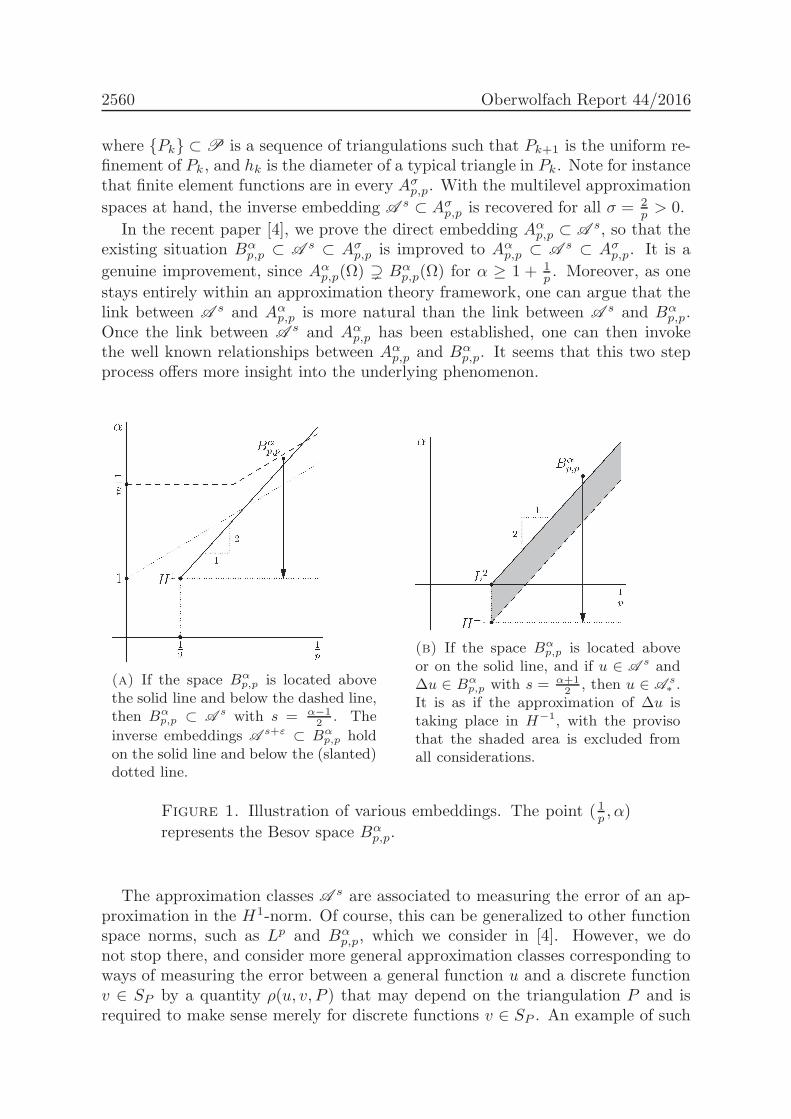
2560 Oberwolfach Report 44/2016
where Pk ⊂ P is a sequence of triangulations such that Pk+1 is the uniform re-finement of Pk, and hk is the diameter of a typical triangle in Pk. Note for instancethat finite element functions are in every Aσ
p,p. With the multilevel approximation
spaces at hand, the inverse embedding A s ⊂ Aσp,p is recovered for all σ = 2
p > 0.
In the recent paper [4], we prove the direct embedding Aαp,p ⊂ A
s, so that theexisting situation Bα
p,p ⊂ A s ⊂ Aσp,p is improved to Aα
p,p ⊂ A s ⊂ Aσp,p. It is a
genuine improvement, since Aαp,p(Ω) ) Bα
p,p(Ω) for α ≥ 1 + 1p . Moreover, as one
stays entirely within an approximation theory framework, one can argue that thelink between A s and Aα
p,p is more natural than the link between A s and Bαp,p.
Once the link between As and Aα
p,p has been established, one can then invokethe well known relationships between Aα
p,p and Bαp,p. It seems that this two step
process offers more insight into the underlying phenomenon.
(a) If the space Bαp,p is located above
the solid line and below the dashed line,then B
αp,p ⊂ A
s with s = α−1
2. The
inverse embeddings As+ε
⊂ Bαp,p hold
on the solid line and below the (slanted)dotted line.
(b) If the space Bαp,p is located above
or on the solid line, and if u ∈ As and
∆u ∈ Bαp,p with s = α+1
2, then u ∈ A
s∗.
It is as if the approximation of ∆u istaking place in H
−1, with the provisothat the shaded area is excluded fromall considerations.
Figure 1. Illustration of various embeddings. The point ( 1p , α)
represents the Besov space Bαp,p.
The approximation classes A s are associated to measuring the error of an ap-proximation in the H1-norm. Of course, this can be generalized to other functionspace norms, such as Lp and Bα
p,p, which we consider in [4]. However, we donot stop there, and consider more general approximation classes corresponding toways of measuring the error between a general function u and a discrete functionv ∈ SP by a quantity ρ(u, v, P ) that may depend on the triangulation P and isrequired to make sense merely for discrete functions v ∈ SP . An example of such

Adaptive Algorithms 2561
an error measure is
ρ(u, v, P ) =
(‖u− v‖2H1 +
∑
τ∈P
(diam τ)2‖f −Πτf‖2L2(τ)
) 12
,
where f = ∆u, and Πτ : L2(τ) → Pd is the L2(τ)-orthogonal projection onto Pd,the space of polynomials of degree not exceeding d. It has been shown in [3] thatif the solution u of the boundary value problem
∆u = f in Ω and u|Ω = 0,
satisfiesmin
P∈P:#P≤Ninf
v∈SP
ρ(u, v, P ) ≤ cN−s,
for all N ≥ #P0 and for some constants c and s > 0, then a typical adaptivefinite element method converges with the rate not slower than s. Moreover, thereare good reasons to consider that the approximation classes A s
∗ defined by thepreceding equation are more attuned to certain practical adaptive finite elementmethods than the standard approximation classes. Obviously, we have A s
∗ ⊂ A s
but we cannot expect the inclusion A s ⊂ A s∗ to hold in general. In [3], an effective
characterization of As∗ was announced as an important pending issue.
The general results in [4] imply a characterization of A s∗ in terms of member-
ships of u and f = ∆u into suitable approximation spaces, which in turn arerelated to Besov spaces. For instance, we show that if u ∈ A s and f ∈ Bα
p,p
with α2 ≥ 1
p − 12 and s = α+1
2 , then u ∈ A s∗ , see Figure 1(b). Note that the
approximation rate s = α+12 is as if we were approximating f in the H−1-norm,
which is illustrated by the arrow downwards. However, the parameters must sat-isfy α
2 ≥ 1p − 1
2 (above or on the solid line), which is more restrictive compared
to α+12 > 1
p − 12 (above the dashed line), the latter being the condition we would
expect if the approximation was indeed taking place in H−1. This situation cannotbe improved in the sense that if α
2 <1p − 1
2 then Bαp,p 6⊂ L2, hence the quantity ρ
would be infinite in general for f ∈ Bαp,p.
References
[1] P. Binev, W. Dahmen, and R. DeVore, Adaptive finite element methods with convergencerates, Numer. Math. 97 (2004), 219–268.
[2] P. Binev, W. Dahmen, R. DeVore, and P. Petrushev, Approximation classes for adaptivemethods, Serdica Math. J., 28 (2002), 391–416.
[3] J. M. Cascon, C. Kreuzer, R. H. Nochetto, and K. G. Siebert, Quasi-optimal convergencerate for an adaptive finite element method, SIAM J. Numer. Anal., 46 (2008), 2524–2550.
[4] T. Gantumur, Convergence Rates of Adaptive Methods, Besov Spaces, and Multilevel Ap-proximation, Found. Comp. Math., (2016), 1–40.
[5] F. D. Gaspoz and P. Morin, Approximation classes for adaptive higher order finite elementapproximation, Math. Comp., 83 (2014), 2127–2160.
[6] R. P. Stevenson, Optimality of a standard adaptive finite element method, Found. Comput.
Math., 7 (2007), 245–269.
2562 Oberwolfach Report 44/2016
Adaptive discretization in Banach spaces with the nonlinearPetrov–Galerkin method
Kristoffer G. van der Zee
(joint work with Ignacio Muga)
This short note reviews some initial results and open problems for the adaptive dis-cretization of linear problems in Banach-space settings with the nonlinear Petrov–Galerkin method. This is relevant to, for example, PDEs with rough data ornonsmooth solutions.
1. The nonlinear Petrov–Galerkin method
In the setting of Banach spaces, consider the linear problem:
Find u ∈ U :⟨Bu, v
⟩V∗,V
=⟨f, v⟩V∗,V
∀v ∈ V ,
where B ∈ L(U;V∗) is a linear continuous operator, f ∈ V∗, U is a Banach spaceand V is a strictly-convex reflexive Banach space with strictly-convex dual V∗.1 Intypical examples, U and V are distinct reflexive Sobolev spaces (e.g., Lp or W 1,p,1 < p <∞).
To ensure well-posedness of the above problem (by the Banach closed-rangetheorem and open-mapping theorem), we assume that B is bounded below, i.e.,
‖Bw‖V∗ ≥ γ‖w‖U ∀w ∈ U ,
for some γ > 0, and that its dual operator has a trivial kernel, i.e., Ker(B∗) = 0.Given a discrete subspace Un ⊂ U, the nonlinear Petrov–Galerkin (NPG) dis-
cretization, proposed in [11], is given by:
(1) Find un ∈ Un :⟨Bwn , J
−1Vm
(f −Bun
)⟩V∗,V
= 0 ∀wn ∈ Un ,
where Vm ⊆ V is a subspace, and JVm : Vm → V∗m is the bijective duality map
for Vm. The duality map for a Banach space X with strictly convex X∗ is a(generally nonlinear) map defined by ‖JX(x)‖X∗ = ‖x‖X and
⟨JX(x), x
⟩X∗,X
=
‖x‖2Xfor all x ∈ X. It is a linear map only in Hilbert spaces, in which case it
coincides with the (linear) Riesz map.
2. Connections and tractability
The NPG method builds on recent ideas in Petrov–Galerkin and residual mini-mization methods: It extends the seminal optimal Petrov–Galerkin methodologyof Demkowicz and Gopalakrishnan [7] to Banach spaces; it provides for a (mono-tone) nonlinear extension of the corresponding mixed formulation, cf. Dahmen etal [6]; and it extends the Lp residual-minimization method of Guermond [10] toarbitrary dual Banach spaces.
1A normed space X is strictly convex iff ‖θx+ (1 − θ)y‖X < 1 for all θ ∈ (0, 1), where x 6= y,and ‖x‖X = ‖y‖X = 1.
Adaptive Algorithms 2563
The case Vm = V corresponds to the ideal setting, and delivers the best ap-proximation in Un as measured in the norm ‖B(·)‖V∗ . The NPG method becomestractable however for discrete Vm. In that case, the (discrete) well-posednessand the quasi-optimality of the NPG method are guaranteed under the follow-ing Fortin compatibility condition for the pair (Un,Vm): There exists a boundedprojection Π : V → Vm such that
(2)⟨Bwn, v −Π(v)
⟩V∗,V
= 0 ∀wn ∈ Un ,
for all v ∈ V. Hence, the NPGmethod needs, in particular, that dimVm ≥ dimUn.Another generalization provided by the NPG method is the following: Upon
choosing a special compatible pair (Un,Vm) for which dimVm = dimUn, onerecovers the standard (linear) Petrov–Galerkin method! See [11] for more details.
3. Adaptive discretization: Challenges
The NPG method is a general discretization method which aims to deliver, withguaranteed stability, near-best approximations to problems in functional settingsbeyond Hilbert spaces, thereby opening up the possibility to address a range ofnew applications. From a theoretical point of view, further research is required,e.g., to clarify how to tackle the Fortin condition (which is likely to be problemdependent), and to devise good solvers for the nonlinear system contained in (1).
Significant research is also needed to develop and understand adaptive dis-cretization strategies with the NPG method. The key ingredient in the efficientadaptive generation of (nested) subspaces Un are a posteriori error estimates.Coincidentally, the NPG method has a natural a posteriori error analysis, whichcan be employed, in standard manners, to generate adaptively-refined subspaces(as in, e.g., adaptive finite element methods):
Theorem (A posteriori error analysis) Assume that the Fortin condi-tion (2) holds. Let un ∈ Un denote the (well-defined) approximation given by theNPG method (1), and let rm := J−1
Vm(f −Bun) ∈ Vm denote its discrete residual
representation. Then
1
‖B‖‖rm‖V ≤ ‖u− un‖U ≤ ‖Π‖γ
‖rm‖V +1
γosc(f) ,
where the data oscillation is defined by osc(f) :=∥∥f (I −Π)
∥∥V∗ .
The proof of this result can be found [11]. It is perhaps striking that thea posteriori result is exactly the same as the one in Hilbert-space settings [4, 1];this is not true for the a priori error analysis, which simplifies in Hilbert spacesbecause of linearity and Kato’s identity for projectors.
The above theorem is a first result that is needed to understand adaptiv-ity. However, since the NPG method is a nonstandard, nonlinear discretizationmethodology, the established theories for the analysis of adaptive methods do notseem to apply. There are many open problems that need to be addressed; we closethis note by mentioning some exciting questions:
2564 Oberwolfach Report 44/2016
• Can one guarantee that a sequence of adaptively-computed approxima-tions un converges to the solution u, and if so, is this convergence optimalwith respect to a suitable adaptive-approximation class (cf. [12, 3, 2])?
• Is it possible to avoid the (intractable) computation of osc(f), e.g., byresorting to suitable (adaptive) data approximation (cf. [5]) or adaptivecomputation of Vm (cf. [6])?
• Can one design optimally-convergent goal-oriented adaptive NPG algo-rithms that aim to efficiently resolve output-quantities of interest (cf. [9])?
• How should one include linearization errors which results from the solutionof the nonlinear discrete system (cf. [8])?
References
[1] C. Carstensen, L. Demkowicz, J. Gopalakrishnan, A posteriori error control for DPG meth-ods, SIAM J. Numer. Anal., 52 (2014), pp. 1335–1353.
[2] C. Carstensen, M. Feischl, M. Page, D. Praetorius, Axioms of adaptivity, Comput. Math.Appl., 67 (2014), pp. 1195–1253.
[3] J. M. Cascon, C. Kreuzer, R. H. Nochetto, K. G. Siebert, Quasi-optimal convergence ratefor an adaptive finite element method, SIAM J. Numer. Anal., 46 (2008), pp. 2524–2550.
[4] A. Cohen, W. Dahmen, G. Welper, Adaptivity and variational stabilization for convection-diffusion equations, M2AN Math. Model. Numer. Anal., 46 (2012), pp. 1247–1273.
[5] A. Cohen, R. DeVore, R. H. Nochetto, Convergence rates of AFEM with H−1 data, Found.Comput. Math., 12 (2012), pp. 671–718.
[6] W. Dahmen, C. Huang, C. Schwab, G. Welper, Adaptive Petrov–Galerkin methods for firstorder transport equations, SIAM J. Numer. Anal., 50 (2012), pp. 2420–2445.
[7] L. Demkowicz, J. Gopalakrishnan, An overview of the Discontinuous Petrov Galerkinmethod, in Recent Developments in Discontinuous Galerkin Finite Element Methods
for Partial Differential Equations: 2012 John H Barrett Memorial Lectures, X. Feng,O. Karakashian and Y. Xing (eds.), pp. 149–180, Springer, (2014)
[8] A. Ern, M. Vohralık, Adaptive inexact Newton methods: A posteriori error control andspeedup of calculations, SIAM News, 46 (2013).
[9] M. Feischl, D. Praetorius, K. G. van der Zee, An abstract analysis of optimal goal-orientedadaptivity, SIAM J. Numer. Anal., 54 (2016), pp. 1523–1448.
[10] J. L. Guermond, A finite element technique for solving first-order PDEs in Lp, SIAM J.Numer. Anal., 42 (2004), pp. 714–737
[11] I. Muga, K. G. van der Zee, Discretization of linear problems in Banach spaces: Residualminimization, nonlinear Petrov–Galerkin, and monotone mixed methods, arXiv:1511.04400[math.NA].
[12] R. Stevenson, Optimality of a standard adaptive finite element method, Found. Comput.Math., 7 (2007), pp. 245–269.
Adaptive Algorithms 2565
Local error analysis of the boundary element method forpolygonal/polyhedral domains
Jens Markus Melenk
(joint work with Markus Faustmann)
Energy projection methods such as many finite element methods (FEM) or bound-ary element methods (BEM) minimize the error in some global norm. Locally, i.e.,on fixed subdomains, the convergence may be better, especially, if the sought so-lution is smoother there. In the context of the FEM, the numerical analyses ofthis setting goes back at least to [4]; subsequent generalizations include [9, 1] andthe references there. These estimates take the following form: The error in thelocal H1-norm is estimated by a local best approximation error in H1 and an er-ror in a weaker norm (L2-norm or negative norm). Significantly fewer works areconcerned with local error estimates for the BEM. The case of smooth curves isstudied in [5, 8], and [7] analyze screen domains. For the case of piecewise smoothgeometries, sharp local error estimates that exploit the maximum local regularityof the solution do not seem to be available. Additionally, the local estimates in[5, 8, 7] focus on the energy norm and do not provide sharp estimates in strongernorms. For the case of Symm’s integral equation, Theorem 1 below presents sharpestimates in the local L2-norm, which is stronger than the local energy norm. Ournumerics illustrate the sharpness of these a priori bounds. Full proofs are given inthe forthcoming paper [3].
Main results. We study polygonal (d = 2) or polyhedral (d = 3) Lipschitz do-main Ω ⊂ Rd with boundary Γ := ∂Ω. An important fact is that for such domainsan elliptic shift theorem for the interior and exterior Dirichlet problem holds inan extended range, which we denote by a parameter αD ∈ (0, 1/2). Specifically,let the ball BRΩ(0) be so large that Ω ⊂ BRΩ(0). Then we require for every
0 < ǫ ≤ αD and both Ω = Ω and Ω = BRΩ(0) \Ω the validity of the shift theorem
(1) ‖u‖H3/2+ǫ(Ω) ≤ Cε ‖f‖H−1/2+ǫ(Ω) ,
where u denotes the solution of −∆u = f in Ω, u = 0 on ∂Ω. We mention thatfor d = 2 the parameter αD can be determined explicitly terms of the largestinterior and exterior angles of the polygon, viz., any αD with 1/2 < αD + 1/2 <miniπ/ωi, π/(2π − ωi), where the ωi are the internal angles of the polygon.
We consider Symm’s integral equation of finding φ ∈ H−1/2(Γ) such that V φ =g, where g ∈ H1/2(Γ) is given and V : H−1/2(Γ) → H1/2(Γ) denotes the single-layer boundary integral operator (see [6, p. 119]).
On a regular quasi-uniform triangulation Th of Γ with mesh size h, we considera lowest order Galerkin discretization in the space of piecewise constant functionson Th, which we denote by S0,0(Th).Theorem 1. Let (1) hold. Let φ ∈ H−1/2(Γ) and φh ∈ S0,0(Th) satisfy theGalerkin orthogonality condition
〈V (φ− φh), ψh〉 = 0 ∀ψh ∈ S0,0(Th).
2566 Oberwolfach Report 44/2016
Let Γ0, Γ be open subsets of Γ with Γ0 ⊂ Γ ( Γ and R := dist(Γ0, ∂Γ) > 0.
Assume φ ∈ L2(Γ). Then,
‖φ− φh‖L2(Γ0)≤ C
(inf
χh∈S0,0(Th)‖φ− χh‖L2(Γ) + ‖φ− φh‖H−1−αD (Γ)
),
where C > 0 depends only on Γ, Γ0, d, R, and the γ-shape regularity of Th.The norm ‖ · ‖H−1−αD (Γ) is the dual norm of ‖ · ‖H1+αD (Γ), which is defined as
‖w‖H1+αD (Γ) := inf‖W‖H3/2+αD (Ω) : W |Γ = w.The key step of the local error analysis of the FEM [4, 9, 1] is a Caccioppoli-
type inequality for discrete harmonic functions. The corresponding estimate forthe BEM is likewise key and stated in the following proposition:
Proposition 1 ([2, Lemma 3.9]). Let ζh ∈ S0,0(Th) and define the potential u :=
V ζh ∈ H1ℓoc(R
d). Let B1 ⊂ B2 be two concentric balls with radii R1 < R2. Thenthere is C > 0 (depending only on R1, R2, and Γ) such that for h sufficiently smallthe following holds: If 〈V ζh, ψh〉 = 0 for all ψh ∈ S0,0(Th) with suppψh ⊂ B2,then
‖∇u‖L2(B1) ≤ C[h‖∇u‖L2(B2) + ‖u‖L2(B2)
].
By assuming the solution φ of V φ = g to be in the Sobolev space H−1/2+α(Γ),α > 0, and to have locally even better Sobolev regularity Hβ , β ∈ [0, 1], we canbe explicit in the local convergence rates:
Corollary 1. Let the assumptions of Theorem 1 be fulfilled. Let Γ ⊂ Γ be a subset
with Γ ( Γ and dist(Γ, ∂Γ) = R > 0. Additionally, assume φ ∈ H−1/2+α(Γ) ∩Hβ(Γ) with α ≥ 0, β ∈ [0, 1]. Then, with a constant C > 0 depending only on
Γ, Γ, d, R, α, β, and the γ-shape regularity of Th,‖φ− φh‖L2(Γ0)
≤ Chmin1/2+α+αD ,β.
The error term ‖φ − φh‖H−1−αD (Γ) in Theorem 1 is treated with a duality ar-gument that utilizes the maximum amount of regularity provided by the shifttheorem given in (1). Therefore, one does not expect that replacing the contribu-tion ‖φ−φh‖H−1−αD (Γ) in Theorem 1 with an even weaker norm (which is possible)leads to improvements in the convergence rate. Indeed, the numerics below showthat our estimates are sharp.
Numerical Example. In order to underline that our local estimates are opti-mal, we study the behavior of the local error on the L-shaped domain in the L2(Γ0)-
norm and theH−1/2(Γ0)-norm, computed by ‖φ‖2H−1/2(Γ0)∼ 〈V (χ0φ), χ0φ〉, where
χ0 is the characteristic function for Γ0 ⊂ Γ. Here, Γ0 is fixed and a union ofelements away from the reentrant corner at the origin. For the L-shaped do-main, we may choose αD = 1/6 − ǫ for any ǫ > 0. We prescribe the solutionu(r, θ) = rα cos(αθ) of Poisson’s equation in polar coordinates. Then, the normalderivative φ = ∂nu solves V φ = (K + 1/2)γ0u with the double layer operator K.We have φ ∈ H−1/2+α(Γ) ∩ H1(Γ0), and with the choice α = 1/6, Corollary 1leads to an expected local rate of O(hα+1/2+αD ) = O(h5/6−ǫ).
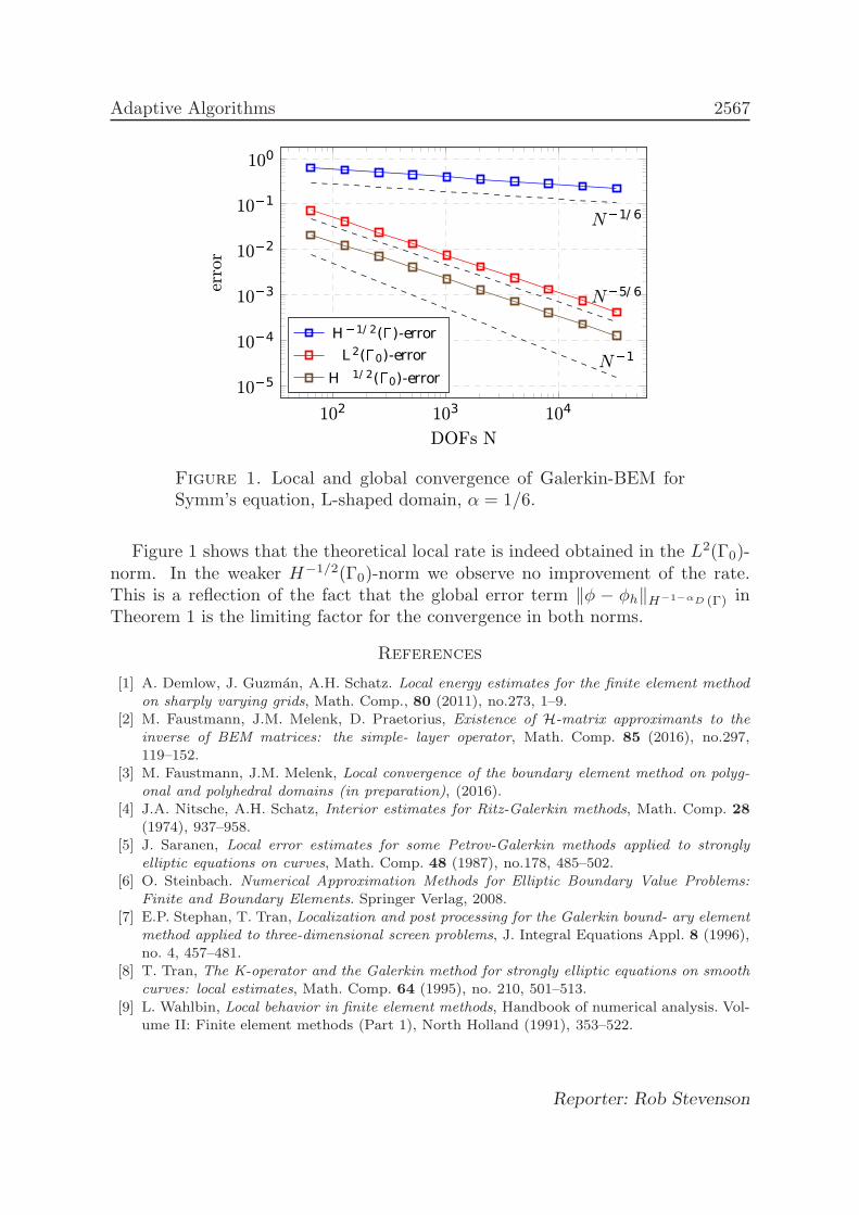
Adaptive Algorithms 2567
102 103 104
105
104
103
102
101
100
N1
N5/ 6
N1/ 6
DOFs N
error
H 1/ 2()-error
L 2(0)-error
H 1/ 2(0)-error
Figure 1. Local and global convergence of Galerkin-BEM forSymm’s equation, L-shaped domain, α = 1/6.
Figure 1 shows that the theoretical local rate is indeed obtained in the L2(Γ0)-norm. In the weaker H−1/2(Γ0)-norm we observe no improvement of the rate.This is a reflection of the fact that the global error term ‖φ − φh‖H−1−αD (Γ) inTheorem 1 is the limiting factor for the convergence in both norms.
References
[1] A. Demlow, J. Guzman, A.H. Schatz. Local energy estimates for the finite element methodon sharply varying grids, Math. Comp., 80 (2011), no.273, 1–9.
[2] M. Faustmann, J.M. Melenk, D. Praetorius, Existence of H-matrix approximants to theinverse of BEM matrices: the simple- layer operator, Math. Comp. 85 (2016), no.297,119–152.
[3] M. Faustmann, J.M. Melenk, Local convergence of the boundary element method on polyg-onal and polyhedral domains (in preparation), (2016).
[4] J.A. Nitsche, A.H. Schatz, Interior estimates for Ritz-Galerkin methods, Math. Comp. 28(1974), 937–958.
[5] J. Saranen, Local error estimates for some Petrov-Galerkin methods applied to stronglyelliptic equations on curves, Math. Comp. 48 (1987), no.178, 485–502.
[6] O. Steinbach. Numerical Approximation Methods for Elliptic Boundary Value Problems:Finite and Boundary Elements. Springer Verlag, 2008.
[7] E.P. Stephan, T. Tran, Localization and post processing for the Galerkin bound- ary elementmethod applied to three-dimensional screen problems, J. Integral Equations Appl. 8 (1996),no. 4, 457–481.
[8] T. Tran, The K-operator and the Galerkin method for strongly elliptic equations on smoothcurves: local estimates, Math. Comp. 64 (1995), no. 210, 501–513.
[9] L. Wahlbin, Local behavior in finite element methods, Handbook of numerical analysis. Vol-ume II: Finite element methods (Part 1), North Holland (1991), 353–522.
Reporter: Rob Stevenson
2568 Oberwolfach Report 44/2016
Participants
Prof. Dr. Peter G. Binev
Department of MathematicsUniversity of South CarolinaColumbia, SC 29208UNITED STATES
Prof. Dr. Zhiqiang Cai
Department of MathematicsPurdue UniversityWest Lafayette, IN 47907-1395UNITED STATES
Prof. Dr. Claudio Canuto
Dipartimento di MatematicaPolitecnico di TorinoCorso Duca degli Abruzzi, 2410129 TorinoITALY
Prof. Dr. Carsten Carstensen
Institut fur MathematikHumboldt-Universitat zu BerlinUnter den Linden 610099 BerlinGERMANY
Prof. Dr. Wolfgang Dahmen
Institut fur Geometrie undPraktische MathematikRWTH AachenTemplergraben 5552056 AachenGERMANY
Prof. Dr. Alan Demlow
Department of MathematicsTexas A & M UniversityCollege Station, TX 77843-3368UNITED STATES
Prof. Dr. Lars Diening
Fachbereich Mathematik/InformatikUniversitat OsnabruckAlbrechtstrasse 28 A49076 OsnabruckGERMANY
Dr. Michael Feischl
School of Mathematics and StatisticsUniversity of New South WalesSydney NSW 2033AUSTRALIA
Dr. Dietmar Gallistl
Institut fur Angewandteund Numerische MathematikKarlsruher Institut fur Technologie(KIT)76128 KarlsruheGERMANY
Dr. Joscha Gedicke
Fakultat fur MathematikUniversitat WienOskar-Morgenstern-Platz 11090 WienAUSTRIA
Dr. Emmanuil H. Georgoulis
Department of MathematicsUniversity of LeicesterUniversity RoadLeicester LE1 7RHUNITED KINGDOM
Friederike Hellwig
Institut fur MathematikHumboldt-Universitat zu BerlinUnter den Linden 610117 BerlinGERMANY
Adaptive Algorithms 2569
Prof. Dr. Jun Hu
School of Mathematical SciencesPeking UniversityNo. 5 Yiheyuan RoadBeijing 100 871CHINA
Dr. Omar Lakkis
Department of MathematicsUniversity of SussexFalmer CampusBrighton BN1 9RHUNITED KINGDOM
Prof. Dr. Jens M. Melenk
Institut fur Analysis und ScientificComputingTechnische Universitat WienWiedner Hauptstrasse 8 - 101040 WienAUSTRIA
Prof. Dr. Neela Nataraj
Department of MathematicsIndian Institute of Technology BombayPowai, Mumbai 400 076INDIA
Prof. Dr. Serge Nicaise
ISTV, LAMAVUniversite de ValenciennesLe Mont Houy59313 Valenciennes Cedex 9FRANCE
Prof. Dr. Daniel Peterseim
Institut fur Numerische SimulationRheinischeFriedrich-Wilhelms-Universitat BonnWegelerstrasse 653115 BonnGERMANY
Prof. Dr. Dirk Praetorius
Institut fur Analysis und ScientificComputingTechnische Universitat WienWiedner Hauptstrasse 8 - 101040 WienAUSTRIA
Dr. Hella Rabus
Institut fur MathematikHumboldt-Universitat zu BerlinUnter den Linden 610099 BerlinGERMANY
Dr. Mira Schedensack
Institut fur Numerische SimulationUniversitat BonnWegelerstraße 653115 BonnGERMANY
Prof. Dr. Rob Stevenson
Korteweg-de Vries InstituutUniversiteit van AmsterdamPostbus 942481090 GE AmsterdamNETHERLANDS
Prof. Dr. Gantumur Tsogtgerel
Department of Mathematics andStatisticsMcGill University805, Sherbrooke Street WestMontreal, P.Q. H3A 2K6CANADA
Dr. Kris G. van der Zee
School of Mathematical SciencesThe University of NottinghamUniversity ParkNottingham NG7 2RDUNITED KINGDOM

2570 Oberwolfach Report 44/2016
Prof. Dr. Marco Verani
Dipartimento di MatematicaPolitecnico di MilanoVia Bonardi 920133 MilanoITALY
Prof. Dr. Martin Vohralik
INRIA RocquencourtDomaine de VoluceauBP 10578153 Le Chesnay CedexFRANCE