Mathematical Foundations of Computing - Stanford Universityweb.stanford.edu/class/archive/cs/cs103/cs103.1126... · Mathematical Foundations of Computing-1 / 74-Mathematical Foundations

Mathematical Foundations of Computing -1 / 74-

Mathematical Foundations of Computing

Preliminary Course Notes

Keith Schwarz

Spring 2012

This is a work-in-progress draft of what I hope will become a full set of course notes for CS103. Right now, the notes only cover up through the end of the first week.

I hope that you find these notes useful! If you have any comments, criticisms, or suggestions, please email me at [email protected]. I'd love to make these notes as good as possible for future quarters.

mailto:[email protected]


Table of ContentsMathematical Foundations of Computing.......................................................................................1Chapter One: Set Theory and Cantor's Theorem.............................................................................4

What is a Set?..............................................................................................................................4Operations on Sets.......................................................................................................................6Special Sets...............................................................................................................................10Set-Builder Notation.................................................................................................................12

Filtering Sets.........................................................................................................................12Transforming Sets.................................................................................................................14

Relations on Sets.......................................................................................................................15Set Equality..........................................................................................................................15Subsets and Supersets...........................................................................................................16The Empty Set and Vacuous Truths......................................................................................17

The Power Set...........................................................................................................................19Cardinality.................................................................................................................................21

What is Cardinality?.............................................................................................................21The Difficulty With Infinite Cardinalities............................................................................22A Formal Definition of Cardinality......................................................................................24

Cantor's Theorem......................................................................................................................28How Large is the Power Set?...............................................................................................28Cantor's Diagonal Argument................................................................................................30Formalizing the Diagonal Argument....................................................................................33Proving Cantor's Theorem....................................................................................................35

Why Cantor's Theorem Matters................................................................................................36The Limits of Computation.......................................................................................................37

What Does This Mean?........................................................................................................38Chapter Summary......................................................................................................................39

Chapter Two: Introduction to Formal Proofs.................................................................................40What is a Proof?........................................................................................................................40

What Can We Assume?........................................................................................................41Direct Proofs.............................................................................................................................41

Proof by Cases......................................................................................................................44Proofs about Sets..................................................................................................................46Lemmas................................................................................................................................49Proofs with Vacuous Truths..................................................................................................53

Indirect Proofs...........................................................................................................................55Logical Implication..............................................................................................................55Proof by Contradiction.........................................................................................................57Rational and Irrational Numbers..........................................................................................61Proof by Contrapositive........................................................................................................64

Chapter Three: Graphs, Functions, and Relations.........................................................................67Chapter Four: The Pigeonhole Principle........................................................................................69Chapter Five: Mathematical Induction..........................................................................................70Chapter Six: Proofs about Programs..............................................................................................71


Chapter Seven: Formal Logic........................................................................................................72

Chapter One: Set Theory and Cantor's Theorem -4 / 74-

Chapter One: Set Theory and Cantor's TheoremOur journey into the realm of mathematics begins with an exploration of a surprisingly nuanced concept: the set. Informally, a set is just a collection of things, whether it's a set of numbers, a set of clothes, a set of nodes in a network, or a set of other sets. Amazingly, given this very simple starting point, it is possible to prove a result known as Cantor's Theorem that provides a striking and profound limit on what problems a computer program can solve. In this introductory chapter, we'll build up some basic mathematical machinery around sets, then will see how the simple notion of asking how big a set can lead to incredible and shocking results.

What is a Set?

Let's begin with a simple definition:

A set is an unordered collection of distinct elements.

What exactly does this mean? Intuitively, you can think of a set as a group of things. Those things must be distinct, which means that you can't have multiple copies of the same object in a set. Additionally, those things are unordered, so there's no notion of a “first” thing in the group, a “second” thing in a group, etc.

We need two additional pieces of terminology to talk about sets:

An element is something contained within a set.

To denote a set, we write the elements of the set within curly braces. For example, the set {1, 2, 3} is a set with three elements: 1, 2, and 3. The set { cat, dog } is a set containing the two elements “cat” and “dog.”

Because sets are unordered collections, the order in which we list the elements of a set doesn't matter. This means that the sets {1, 2, 3}, {2, 1, 3}, and {3, 2, 1} are all descriptions of exactly the same set. Also, because sets are unordered collections of distinct elements, no element can appear more than once in the same set. In particular, this means that if we write out a set like {1, 1, 1, 1, 1}, it's completely equivalent to writing out the set {1}, since sets can't contain duplicates. Similarly, {1, 2, 2, 2, 3} and {3, 2, 1} are the same set, since ordering doesn't matter and duplicates are ignored.

When working with sets, we are often interested in determining whether or not some object is an element of a set. We use the notation x ∈ S to denote that x is an element of the set S. For example, we would write that 1 {1, 2, 3}, or that cat { cat, dog }. If spoken aloud, you'd∈ ∈ read x S as “x is an element of S.” Similarly, we use the notation x ∈ ∉ S to denote that x is not an element of S. So, we would have 1 {2, 3, 4}, dog {1, 2, 3}, and ibex {cat, dog}. You∉ ∉ ∉ can read x S as “x is not an element of S.”∉


Sets appear almost everywhere in mathematics because they capture the very simple notion of a group of things. If you'll notice, there aren't any requirements about what can be in a set. You can have sets of integers, set of real numbers, sets of lines, sets of programs, and even sets of other sets. Through the remainder of your mathematical career, you'll see sets used as building blocks for larger and more complicated objects.

As we just mentioned, it's possible to have sets that contain other sets. For example, the set { {1, 2}, 3 } is a set containing two elements – the set {1, 2} and the number 3. There's no requirement that all of the elements of a set have the same “type,” so a single set could contain numbers, animals, colors, and other sets without worry. That said, when working with sets that contain other sets, it's important to note what the elements of that set are. For example, consider the set

{{1, 2}, {2, 3}, 4}

has just three elements: {1, 2}, {2, 3}, and 4. This means that

{1, 2} {{1, 2}, {2, 3}, 4}∈

{2, 3} {{1, 2}, {2, 3}, 4}∈

4 {{1, 2}, {2, 3}, 4}∈

However, it is not true that 1 {{1, 2}, {2, 3}, 4}. Although {{1, 2}, {2, 3}, 4} contains the set∈ {1, 2} which in turn contains 1, 1 itself is not an element of {{1, 2}, {2, 3}, 4}. In a sense, set containment is “opaque,” in that it just asks whether the given object is directly contained within the set, not whether it is contained with that set, a set contained within that set, etc. Consequently, we have that

1 {{1, 2}, {2, 3}, 4}∉

2 {{1, 2}, {2, 3}, 4}∉

3 {{1, 2}, {2, 3}, 4}∉

But we do have that

4 {{1, 2}, {2, 3}, 4}∈

Because 4 is explicitly listed as a member of the set.

In the above example, it's fairly time-consuming to keep writing out the set {{1, 2}, {2, 3}, 4} over and over again. Commonly, we'll assign names to mathematical objects to make it easier to refer to them in the future. In our case, let's call this set “S.” Mathematically, we can write this out as

S = {{1, 2}, {2, 3}, 4}

Given this definition, we can rewrite all of the above discussion much more compactly:

{1, 2} ∈ S

{2, 3} ∈ S

4 ∈ S

1 ∉ S


2 ∉ S

3 ∉ S

Throughout this book, and in the mathematical world at large, we'll be giving names to things and then manipulating and referencing those objects through those names. Hopefully you've used variables before when programming, so I hope that this doesn't come as too much of a surprise.

Before we move on and begin talking about what sorts of operations we can perform on sets, we need to introduce a very special set that we'll be making extensive use of: the empty set.

The empty set is the set that does not contain any elements.

It may seem a bit strange to think about a collection of no things, but that's precisely what the empty set is. You can think of the empty set as representing a group that doesn't have anything in it. One way that we could write the empty set is as { }, indicating that it's a set (the curly braces), but that this set doesn't contain anything (the fact that there's nothing in-between them!) However, in practice this notation is not used, and we use the special symbol Ø to denote the empty set.

The empty set has the nice property that there's nothing in it, which means that for any object x that you ever find anywhere, x Ø. This means that the statement x Ø is always false.∉ ∈

Let's return to our earlier discussion of sets containing other sets. It's possible to build sets that contain the empty set. For example, the set { Ø } is a set with one element in it, which is the empty set. Thus we have that Ø { Ø }. More importantly, note that Ø and { Ø } are ∈ not the same set. Ø is a set that contains no elements, while { Ø } is a set that does indeed contain an element, namely the empty set. Be sure that you understand this distinction!

Operations on Sets

Sets represent collections of things, and it's common to take multiple collections and ask questions of them. What do the collections have in common? What do they have collectively? What does one set have that the other does not? These questions are so important that mathematicians have rigorously defined them and given them fancy mathematical names.

First, let's think about finding the elements in common between two sets. Suppose that I have two sets, one of US coins and one of chemical elements. This first set, which we'll call C, is

C = { penny, nickel, dime, quarter, half-dollar, dollar }

and the second set, which we'll call E, contains these elements:

E = { hydrogen, helium, lithium, beryllium, boron, carbon, …, ununseptium }

(Note the use of the ellipsis here. It's often acceptable in mathematics to use ellipses when there's a clear pattern present, as in the above case where we're listing the elements in order. Usually, though, we'll invent some new symbols we can use to more precisely describe what we mean.)


The sets C and E happen to have one element in common: nickel, since

nickel ∈ C

and

nickel ∈ E

However, some sets may have a larger overlap. For example, consider the sets {1, 2, 3} and {1, 3, 5}. These sets have both 1 and 3 in common. Other sets, on the other hand, might not have anything in common at all. For example, the sets {cat, dog, ibex} and {1, 2, 3} have no elements in common.

Since sets serve to capture the notion of a collection of things, we might think about the set of elements that two sets have in common. In fact, that's a perfectly reasonable thing to do, and it goes by the name intersection:

The intersection of two sets S and T, denoted S ∩ T, is the set of elements contained in both S and T.

For example, {1, 2, 3} ∩ {1, 3, 5} = {1, 3}, since the two sets have exactly 1 and 3 in common. Using the set C of currency and E of chemical elements from earlier, we would say that C ∩ E = {nickel}.

But what about the intersection of two sets that have nothing in common? This isn't anything to worry about. Let's take an example: what is {cat, dog, ibex} ∩ {1, 2, 3}? If we consider the set of elements common to both sets, we get the empty set Ø, since there aren't any common elements between the two sets.

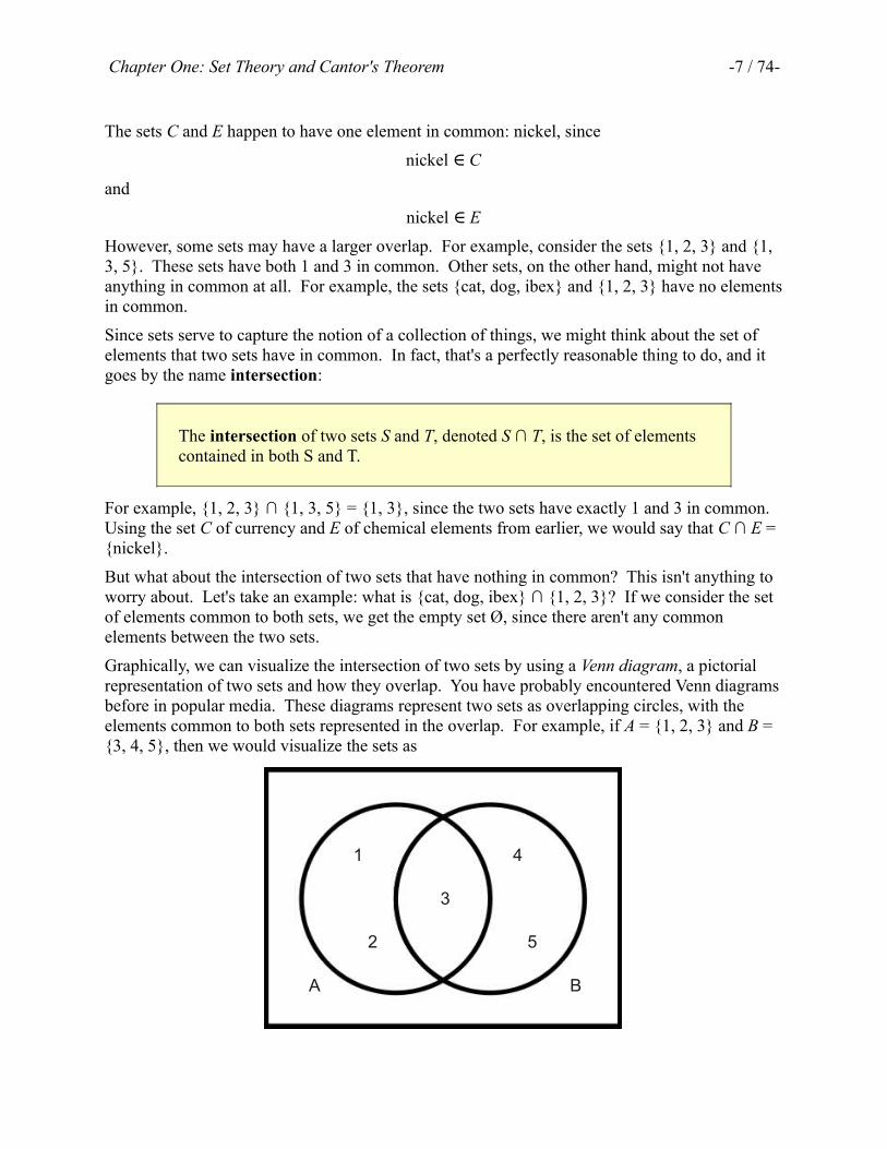
Graphically, we can visualize the intersection of two sets by using a Venn diagram, a pictorial representation of two sets and how they overlap. You have probably encountered Venn diagrams before in popular media. These diagrams represent two sets as overlapping circles, with the elements common to both sets represented in the overlap. For example, if A = {1, 2, 3} and B = {3, 4, 5}, then we would visualize the sets as

A B

1

2

4

5

3


Given a Venn diagram like this, the intersection A ∩ B is the set of elements in the intersection, which in this case is {3}.

Just as we may be curious about the elements two sets have in common, we may also want to ask what elements two sets contain collectively. For example, given the sets A and B from above, we can see that, collectively, the two sets contain 1, 2, 3, 4, and 5. Mathematically, the set of elements held collectively by two sets is called the union:

The union of two sets A and B, denoted A ∪ B, is the set of all elements contained in either of the two sets.

Thus we would have that {1, 2, 3} {3, 4, 5} = {1, 2, 3, 4, 5}. Note that, since sets are∪ unordered collections of distinct elements, that it would also have been correct to write {1, 2, 3, 3, 4, 5} as the union of the two sets, since {1, 2, 3, 4, 5} and {1, 2, 3, 3, 4, 5} describe the same set. That said, to eliminate redundant redundancy, typically we'd prefer to write out {1, 2, 3, 4, 5} since it gets the same message across in smaller space.

The symbols for union ( ) and intersection (∩) are similar to one another, and it's often easy to∪ get them confused. A useful mnemonic is that the symbol for union looks like a U, so you can think of the nion of two sets.∪

An important (but slightly pedantic) point is that can only be applied to two sets. This means∪ that although

{1, 2, 3} 4∪

might intuitively be the set {1, 2, 3, 4}, mathematically this statement isn't meaningful because 4 isn't a set. If we wanted to represent the set formed by taking the set {1, 2, 3} and adding 4 to it, we would represent it by writing

{1, 2, 3} {4}∪

Now, since both of the operands are sets, the above expression is perfectly well-defined. Similarly, it's not mathematically well-defined to say

{1, 2, 3} ∩ 3

because 3 is not a set. Instead, we should write

{1, 2, 3} ∩ {3}

Another important point to clarify when working with union or intersection is how they behave when applied to sets containing other sets. For example, what is the value of the following expression?

{{1, 2}, {3}, {4}} ∩ {{1, 2, 3}, {4}}

When computing the intersection of two sets, all that we care about is what elements the two sets have in common. Whether those elements themselves are sets or not is irrelevant. Here, for example, we can list off the elements of the two sets {{1, 2}, {3}, {4}} and {{1, 2, 3}, {4}} as follows:


{1, 2} {{1, 2}, {3}, {4}}∈ {1, 2, 3} {{1, 2, 3}, {4}}∈

{3} {{1, 2}, {3}, {4}}∈ {4} {{1, 2, 3}, {4}}∈

{4} {{1, 2, 3}, {4}}∈

Looking at these two lists of elements, we can see that the only element that the two sets have in common is the element {4}. As a result, we have that

{{1, 2}, {3}, {4}} ∩ {{1, 2, 3}, {4}} = {{4}}

That is, the set of just one element, which is the set containing 4.

You can think about computing the intersection of two sets as the act of “peeling off” just the outermost braces from the two sets, leaving all the elements undisturbed. Then, looking at just those elements, find the ones in common to both sets, and put all of those elements back together.

The union of two sets works similarly. So, if we want to compute

{{1, 2}, {3}, {4}} {{1, 2, 3}, {4}}∪

We would “peel off” the outer braces to find that the first set contains {1, 2}, {3}, and {4} and that the second set contains {1, 2, 3} and {4}. If we then gather all of these together into a set, we get the result that

{{1, 2}, {3}, {4}} {{1, 2, 3}, {4}} = {{1, 2}, {3}, {1, 2, 3}, {4}}∪

Given two sets, we can find what they have in common by finding their intersection and can find what they have collectively by using the union. But both of these operations are symmetric; it doesn't really matter what order the sets are in, since A ∪ B = B ∪ A and A ∩ B = B ∩ A. (If this doesn't seem obvious, try out a couple of examples and see if you notice anything). In a sense, the union and intersection of two sets don't have a “privileged” set. However, at times we might be interested in learning about how one set differs from another. Suppose that we have two sets A and B and want to find the elements of A that don't appear in B. For example, given the sets A = {1, 2, 3} and B = {3, 4, 5}, we would note that the elements 1 and 2 are unique to A and don't appear anywhere in B, and that 4 and 5 are unique to B and don't appear in A. We can capture this notion precisely with the set difference operation:

The set difference of A and B, denoted A – B or A \ B, is the set of elements contained in A but not contained in B.

Note that there are two different notations for set difference. In this book we'll use the minus sign to indicate set subtraction, but other authors use the slash for this purpose. You should be comfortable working with both.

As an example of a set difference, {1, 2, 3} – {3, 4, 5} = {1, 2}, because 1 and 2 are in {1, 2, 3} but not {3, 4, 5}. Note, however, that {3, 4, 5} – {1, 2, 3} = {4, 5}, because 4 and 5 are in {3, 4, 5} but not {1, 2, 3}. Set difference is not symmetric. It's also possible for the difference of two


sets to contain nothing at all, which would happen if everything in the first set is also contained in the second set. For instance, {1, 2, 3} – {1, 2, 3, 4} = Ø, since every element of {1, 2, 3} is also contained in {1, 2, 3, 4}.

There is one final set operation that we will touch on for now. Suppose that you and I travel the world and each maintain a set of the places that we went. If we meet up to talk about our trip, we'd probably be most interested to tell each other about the places that one of us had gone but the other hadn't. Let's say that set A is the set of places I have been and set B is the set of places that you've been. If we take the set A – B, this would give the set of places that I have been that you hadn't, and if you take the set B – A it would give the set of places that you have been that I hadn't. These two sets, taken together, are quite interesting, because they represent fun places to talk about, since one of us would always be interested in hearing what the other had to say. Using just the operators we've talked about so far, we could describe this set as (B – A) (∪ A – B). For simplicity, though, we usually define one final operation on sets that makes this concept easier to convey: the symmetric difference.

The set symmetric difference of two sets A and B, denoted A Δ B, is the set of elements that are contained in exactly one of A or B, but not both.

For example, {1, 2, 3} Δ {3, 4, 5} = {1, 2, 4, 5}, since 1 and 2 are in {1, 2, 3} but not {3, 4, 5} and 4 and 5 are in {3, 4, 5} but not {1, 2, 3}.

Special Sets

So far, we have described sets by explicitly listing off all of their elements: for example, {cat, dog, ibex}, or {1, 2, 3}. But what if we wanted to consider a collection of things that is too big to be listed off this way? For example, consider all the integers, of which there are infinitely many. Could we gather them together into a set? What about the set of all possible English sentences, which is also infinitely huge? Can we make a set out of them?

It turns out that the answer to both of these questions is “yes,” and sets can contain infinitely many elements. But how would we describe such a set? Let's begin by trying to describe the set of all integers. We could try writing this set as

{…, -2, -1, 0, 1, 2, … }

which does indeed convey our intention. However, this isn't mathematically rigorous. When working with complex mathematics, it's important that we be very precise with our notation. To standardize terminology, mathematicians have invented a special symbol used to denote the set of all integers: the symbol .ℤ

The set of all integers, denoted ℤ, is the set = {…, -2, -1, 0, 1, 2, …}ℤ

For example, 0 , -137 , and 42 , but 1.37 , cat , and {1, 2, 3} .∈ℤ ∈ℤ ∈ℤ ∉ℤ ∉ℤ ∉ℤ


Since really is the set of all integers, all of the set operations we've developed so far apply to it.ℤ For example, we could consider the set ∩ {1, 1.5, 2, 2.5}, which is the set {1, 2}. We can alsoℤ compute the union of and some other set. For example, {1, 2, 3} is the set , since 1 ℤ ℤ∪ ℤ ∈

, 2 , and 3ℤ ∈ℤ ∈ .ℤ

You might be wondering – why ? This is from the German word “zahlen,” meaningℤ “numbers.” Much of modern mathematics has its history in Germany, so many terms that we'll encounter in the course of this book (for example, “Entscheidungsproblem”) come from German. Much older terms tend to come from Latin or Greek, while results from the 8th through 13th

centuries are often Arabic (for example, “algebra” derives from the title كتاب المختصر في حساب الجبر of a book written in the 9th century by Persian mathematician al-Khwarizmi, whose name والمقابلةis the source of the word “algorithm.”) It's interesting to see how the languages used in mathematics parallel the dominant world power at the time of the discovery.

While in mathematics the integers appear just about everywhere, in computer science they don't arise as frequently as you might expect. Most languages don't allow for negative array indices. Strings can't have a negative number of characters in them. A loop never runs -3 times. More commonly, in computer science, we find ourselves working with just the numbers 0, 1, 2, 3, …, etc. These numbers are called the natural numbers, and represent answers to questions of the form “how many?” Because natural numbers are so ubiquitous in computing, the set of all natural numbers is particularly important:

The set of all natural numbers, denoted ℕ, is the set ℕ = {0, 1, 2, 3, …}

For example, 0 ∈ℕ, 137 ∈ℕ, but -3 ∉ℕ, 1.1 ∉ℕ, and {1, 2} ∉ℕ.

The natural numbers arise frequently in computing as ways of counting loop iterations, the number of nodes in a binary tree, the number of instructions executed by a program, etc.

Before we move on, I should point out that while there is a definite consensus on what is, thereℤ is not a universally-accepted definition of ℕ. Some mathematicians treat 0 as a natural number, while others do not. Thus you may find that some authors consider

ℕ = {0, 1, 2, 3, … }

while others treat ℕ as

ℕ = {1, 2, 3, … }

For the purposes of this book, we will treat 0 as a natural number, so

• the smallest natural number is 0, and (appropriately)

• 0 ∈ .ℕ

In some cases we may want to consider the set of natural numbers other than zero. We will denote this set ℕ⁺.


The set of positive natural numbers ℕ⁺ is the set ℕ⁺ = {1, 2, 3, …}

Thus 137 ∈ , but 0 ℕ ∉ℕ⁺.

There are other important sets that arise frequently in mathematics and that will appear from time to time in our exploration of the mathematical foundations of computing. We should consider the set of real numbers, numbers representing arbitrary measurements. For example, you might be 1.7234 meters tall, or weigh 70.22 kilograms. Numbers like π and e are real numbers, as are numbers like the square root of two. The set of all real numbers is so important in mathematics that we give it a special symbol.

The set of all real numbers is denoted ℝ.

The sets ℕ, , and are all quite different from the other sets we've seen so far in that theyℤ ℝ contain infinitely many elements. We will return to this topic later, but we do need one final pair of definitions:

A finite set is a set containing only finitely many elements. An infinite set is a set containing infinitely many elements.

Set-Builder Notation

Filtering Sets

So far, we have seen how to use the primitive set operations (union, intersection, difference, and symmetric difference) to combine together sets into other sets. However, more commonly, we are interested in defining a set not by combining together existing sets, but by gathering together all objects that share some common property. It would be nice, for example, to be able to just say something like “the set of all even numbers” or “the set of legal C programs.” For this, we have a tool called set-builder notation which allows us to define a set by describing some property common to all of the elements of that set.

Before we go into a formal definition of set-builder notation, let's see some examples. First, here's how we might define the set of even natural numbers:

{ n | n ∈ℕ and n is even }

We could define the set of positive real numbers this way:

{ x | x and ∈ℝ x > 0 }

Or we could define the set of legal C programs this way:

{ p | p is a legal C program }


If you'll notice, each of these sets is defined using the following pattern:

{ variable | conditions on that variable }

Let's dissect each of the above sets one at a time to see what they mean and how to read them. First, we defined the set of even natural numbers this way:

{ n | n ∈ℕ and n is even }

You would read this aloud as “the set of all n, where n is a natural number and n is even.” In other words, treat the vertical bar as the word “where” or “such that.” Here, this definition says that this is the set formed by taking every choice of n where n ∈ℕ (that is, n is a natural number) and n is even. Consequently, this is the set {0, 2, 4, 6, 8, …}.

The set

{ x | x and ∈ℝ x > 0 }

Can similarly be read off as “the set of all x where x is a real number and x is greater than zero,” which filters the set of real numbers down to just the positive real numbers.

Of the sets listed above, this set was the least mathematically precise:

{ p | p is a legal C program }

However, it's a perfectly reasonable way to define a set: we just gather up all the legal C programs (of which there are infinitely many) and put them into a single set.

When using set-builder notation, the name of the variable chosen does not matter. This means that all of the following are equivalent to one another:

{ x | x and ∈ℝ x > 0 }

{ y | y and ∈ℝ y > 0 }

{ z | z and ∈ℝ z > 0 }

Using set-builder notation, it's actually possible to define many of the special sets from the previous section in terms of one another. For example, we can define the set ℕ as follows:

ℕ = { x | x and ∈ℤ x ≥ 0 }

That is, the set of all natural numbers (ℕ) is the set of all x such that x is an integer and x is nonnegative. This precisely matches our intuition about what the natural numbers ought to be. Similarly, we can define the set ℕ as⁺

ℕ⁺ = { n | n ∈ℕ and n ≠ 0 }

Since this describes the set of all n such that n is a nonzero natural number.

So far, all of the examples above with set-builder notation have started with an infinite set and ended with an infinite set. However, set-builder notation can be used to construct finite sets as well. For example, the set

{ n | n ∈ℕ, n is even, and n < 10 }

has just five elements: 0, 2, 4, 6, and 8.


To formalize our definition of set-builder notation, we need to introduce the notion of a predicate:

A predicate is a statement about some object x that is either true or false.

For example, the statement “x < 0” is a predicate that is true if x is less than zero and false otherwise. The statement “x is an even number” is a predicate that is true if x is an even number and is false otherwise. We can build far more elaborate predicates as well – for example, the predicate “p is a legal C program that prints out a random number” would be true for C programs that print random numbers and false otherwise. Interestingly, it's not required that a predicate be checkable by a computer program. As long as a predicate always evaluates to either true or false – regardless of how we'd actually go about verifying which of the two it was – it's a valid predicate.

Given our definition of a predicate, we can formalize the definition of set-builder notation here:

The set { x | P(x) } is the set of all x such that P(x) is true.

It turns out that allowing us to define sets this way can, in some cases, lead to paradoxical sets, sets that cannot possibly exist. We'll discuss this later on when we talk about Russell's Paradox. However, in practical usage, it's almost universally safe to just use this simple set-builder notation.

Transforming Sets

You can think of this version of set-builder notation as some sort of filter that is used to gather together all of the objects satisfying some property. However, it's also possible to use set-builder notation as a way of applying a transformation to the elements of one set to convert them into a different set. For example, suppose that we want to describe the set of all perfect squares – that is, natural numbers like 0 = 02, 1 = 12, 4 = 22, 9 = 32, 16 = 42, etc. Using set-builder notation, we can do so, though it's a bit awkward:

{ n | there is some m ∈ℕ such that n = m2 }

That is, the set of all numbers n where, for some natural number m, n is the square of m. This feels a bit awkward and forced, because we need to describe some property that's shared by all the members of the set, rather than the way in which those elements are generated. As a computer programmer, you would probably be more likely to think about the set of perfect squares more constructively by showing how to build the set of perfect squares out of some other set. In fact, this is so common that there is a variant of set-builder notation that does just this. Here's an alternative way to define the set of all perfect squares:

{ n2 | n ∈ℕ }


This set can be read as “the set of all n2, where n is a natural number.” In other words, rather than building the set by describing all the elements in it, we describe the set by showing how to apply a transformation to all objects matching some criterion. Here, the criterion is “n is a natural number,” and the transformation is “compute n2.”

As another example of this type of notation, suppose that we want to build up the set of the numbers 0, ½, 1, 3/2, 2, 4/2, etc. out to infinity. Using the simple version of set-builder notation, we could write this set as

{ x | there is some n ∈ℕ such that x = n / 2 }

That is, this set is the set of all numbers x where x is some natural number divided by two. This feels forced, and so we might use this alternative notation instead:

{ n / 2 | n ∈ℕ }

That is, the set of numbers of the form n / 2, where n is a natural number. Here, we transform the set ℕ by dividing each of its elements by two.

It's possible to perform transformations on multiple sets at once when using set-builder notation. For example, let's let the set A = {1, 2, 3} and the set B = {10, 20, 30}. Then consider the following set:

C = { a + b | a ∈ A and b ∈ B }

This set is defined as follows: for any combination of an element a ∈ A and an element b ∈ B, the set C contains the number a + b. For example, since 1 ∈ A and 10 ∈ B, the number 1 + 10 = 11 must be an element of C. It turns out that since there are three elements of A and three elements of B, there are nine possible combinations of those elements:

10 20 30

1 11 21 31

2 12 22 32

3 13 23 33

This means that our set C is

C = { a + b | a ∈ A and b ∈ B } = { 11, 12, 13, 21, 22, 23, 31, 32, 33 }

Relations on Sets

Set Equality

We now have ways of describing collections and of forming new collections out of old ones. However, we don't (as of yet) have a way of comparing different collections. How do we know if two sets are equal to one another?

As mentioned earlier, a set is an unordered collection of distinct elements. We say that two sets are equal if they have exactly the same elements as one another.


If A and B are sets, then A = B precisely when they have the same elements as one another. This definition is sometimes called the axiom of extensionality.

For example, under this definition, {1, 2, 3} = {2, 3, 1} = {3, 1, 2}, since all of these sets have the same elements. Similarly, {1} = {1, 1, 1}, because both sets have the same elements (remember that a set either contains something or it does not, so duplicates are not allowed). This also means that

ℕ = { x | x and ∈ℤ x ≥ 0 }

since the sets have the same elements. It is important to note that the manner in which two sets are described has absolutely no bearing on whether or not they are equal; all that matters are what the two sets contain. In other words, it's not what's out the outside (the description of the sets) that counts; it's what's on the inside (what those sets actually contain).

Because two sets are equal precisely when they contain the same elements, we can get a better feeling for why we call Ø the empty set as opposed to an empty set (that is, why there's only one empty set, as opposed to a whole bunch of different sets that are all empty). The reason for this is that, by our definition of set equality, two sets are equal precisely when they contain the same elements. This means that if you take any two sets that are empty, they must be equal to one another, since they contain the same elements (namely, no elements at all).

Subsets and Supersets

Suppose that you're organizing your music library. You can think of one set M as consisting of all of the songs that you own. Some of those songs are songs that you actually like to listen to, which we could denote F for “Favorite.” If we think about the relationship between the sets M and F you can quickly see that M contains everything that F contains, since M is the set of all songs you own while F is only your favorite songs. It's possible that F = M, if you only own your favorite songs, but in all likelihood your music library probably contains more songs than just your favorites. In this case, what is the relation between M and F? Since M contains everything that F does, plus (potentially) quite a lot more, we say that M is a superset of F. Conversely, F is a subset of M. We can formalize these definitions below:

A set A is a subset of another set B if every element of A is also contained in B. In other words, A is a subset of B precisely if every time x ∈ A, then x

∈ B is true. If A is a subset of B, we write A ⊆ B.

If A ⊆ B (that is, A is a subset of B), then we say that B is a superset of A. We denote this by writing B ⊇ A.


For example, {1, 2} {1, 2, 3}, since every element of {1, 2} is also an element of {1, 2, 3};⊆ specifically, 1 {1, 2, 3} and 2 {1, 2, 3}. Also, {4, 5, 6} {4} because every element of {4}∈ ∈ ⊇ is an element of {4, 5, 6}, since 4 {4, 5, 6}. Additionally, we have that ∈ ℕ , since every⊆ℤ natural number is also an integer, and , since every integer is also a real number.ℤ⊆ℝ

Given any two sets, there's no guarantee that one of them must be a subset of the other. For example, consider the sets {1, 2, 3} and {cat, dog, ibex}. In this case, neither set is a subset of the other, and neither set is a superset of the other.

By our definition of a subset, any set A is a subset of itself, because it's fairly obviously true that every element of A is also an element of A. For example, {cat, dog, ibex} {cat, dog, ibex}⊆ because cat {cat, dog, ibex}, dog {cat, dog, ibex}, and ibex {cat, dog, ibex}. Sometimes∈ ∈ ∈ when talking about subsets and supersets of a set A, we want to exclude A itself from consideration. For this purpose, we have the notion of a strict subset and strict superset:

A set A is a strict subset of B if A ⊆ B and A ≠ B. If A is a strict subset of B, we denote this by writing A ⊂ B.

If A ⊂ B, we say that B is a strict superset of A. In this case, we write B ⊃ A.

For example, {1, 2} {1, 2, 3} because {1, 2} {1, 2, 3} and {1, 2} ≠ {1, 2, 3}. However, {1,⊂ ⊆ 2, 3} is not a strict subset of itself.

The Empty Set and Vacuous Truths

How does the empty set Ø interact with subsets? Consider any set S. Is the empty set a subset of S? Recall our definition of subset:

A B precisely when every element of A is also an element of B.⊆

The empty set doesn't contain any elements, so how does it interact with the above claim? If we plug Ø and the set S into the above, we get the following:

Ø S if every element of Ø is an element of S.⊆

Take a look at that last bit - “if every element of Ø is an element of S.” What does this mean here? After all, there aren't any elements of Ø, because Ø doesn't contain any elements! Given this, is the above statement true or false? There are two ways we can think about this:

1. Since Ø contains no elements, the claim “every element of Ø is an element of S” is false, because we can't find a single example of an element of Ø that is contained in S.

2. Since Ø contains no elements, the claim “every element of Ø is an element of S” is true, because we can't find a single example of an element of Ø that isn't contained in S.


The question boils down to where the burden of proof is. If we go with the first line of reasoning, we would say that if every element of Ø is also an element of S, then we should be able to find some specific example of an element of Ø that's also an element of S to substantiate the claim. Of course, there aren't any elements of Ø at all, so we can't find the example we're looking for. We'd be forced to admit that Ø is not a subset of S.

On the other hand, we could take the second line of reasoning, which is more in the spirit of an “innocent until proven guilty” argument that says that we should consider Ø to be a subset of S because we can't find any counterexamples that would disprove it. In particular, if it turns out that Ø isn't a subset of S, then we should be able to find some example of an element of Ø that isn't contained in S. Since Ø doesn't contain any elements, we can't find this counterexample, and so we'd be forced to admit that Ø actually is a subset of S.

So which line of reasoning ends up being correct? It turns out that it's the second of these two approaches, and indeed it is true that Ø ⊆ S. To understand why, we need to introduce the idea of a vacuous truth. Informally, a statement is vacuously true if it's true simply because it doesn't actually assert anything. For example, consider the statement “if I am a dinosaur, then the moon is on fire.” This statement is completely meaningless, since the statement “I am a dinosaur” is false. Consequently, the statement “if I am a dinosaur, then the moon is on fire” doesn't actually assert anything, because I'm not a dinosaur. Similarly, consider the statement “if 1 = 0, then 3 = 5.” This too doesn't actually assert anything, because we know that 1 ≠ 0.

Interestingly, mathematically speaking, the statements “if I am a dinosaur, then the moon is on fire” and “if 1 = 0, then 3 = 5” are both considered true statements! They are called vacuously true because although they're considered true statements, they're meaningless true statements that don't actually provide any new information or insights. More formally:

The statement “if P, then Q” is vacuously true if P is always false.

There are many reasons to argue in favor of or against vacuous truths. As you'll see later on as we discuss formal logic, vacuous truth dramatically simplifies many arguments and makes it possible to reason about large classes of objects in a way that more naturally matches our intuitions. That said, it does have its idiosyncrasies, as it makes statements that are meaningless, such as “if 1 = 0, then 5 = 3” true.

Let's consider another example: Are all unicorns pink? Well, that's an odd question – there aren't any unicorns in the first place, so how could we possibly know what color they are? But, if you think about it, the statement “all unicorns are pink” should either be true or false.1 Which one is it? One option would be to try rewriting the statement “all unicorns are pink” in a slightly different manner – instead, let's say “if x is a unicorn, then x is pink.” This statement conveys exactly the same idea as our original statement, but is phrased as an “if … then” statement. When we write it this way, we can think back to the definition of a vacuous truth. Since the

1 In case you're thinking “but it could be neither true nor false!,” you are not alone! At the turn of the 20th century, a branch of logic arose called intuitionistic logic that held as a tenet that not all statements are true or false – some might be neither. In intuitionistic logic, there is no concept of a vacuous truth, and statements like “if I am a dinosaur, then the moon is on fire” would simply neither be true nor false. Intuitionistic logic has many applications in computer science, but has generally fallen out of favor in the mathematical community.


statement “x is a unicorn” is never true – there aren't any unicorns! – then the statement “if x is a unicorn, then x is pink” ends up being a true statement because it's vacuously true. More generally:

The statement “Every X has property Y” is (vacuously) true if there are no X's.

Let's return to our original question: is Ø a subset of any set S? Recall that Ø is a subset of S if every element of Ø is also an element of S. But the statement “every element of Ø is an element of S” is vacuously true, because there are no elements of Ø! As a result, we have that

For any set S, Ø ⊆ S.

This means that Ø {1, 2, 3}, Ø {cat, dog, ibex}, Ø ⊆ ⊆ ⊆ℕ, and even Ø Ø.⊆

The Power Set

Given any set S, we know that some sets are subsets of S (there's always at least Ø as an option), while others are not. For example, the set {1, 2} has four subsets:

• Ø, which is a subset of every set,

• {1}

• {2}

• {1, 2}, since every set is a subset of itself.

We know that sets can contain other sets, so we may want to think about the set that contains all four of these subsets as elements. This is the set

{Ø, {1}, {2}, {1, 2}}

More generally, we can think about taking an arbitrary set S and listing off all its subsets. For example, the subsets of {1, 2, 3} are

Ø{1}{2}{3}

{1, 2}{1, 3}{2, 3}

{1, 2, 3}

Note that there are eight subsets here. The subsets of {1, 2, 3, 4} are


Ø

{1}{2}{3}{4}

{1, 2}{1, 3}{1, 4}{2, 3}{2, 4}{3, 4}

{1, 2, 3}{1, 2, 4}{1, 3, 4}{2, 3, 4}

{1, 2, 3, 4}

Note that there are 16 subsets here. In some cases there may be infinitely many subsets – for instance, the set ℕ has subsets Ø, then infinitely many subsets with just one element ({0}, {1}, {2}, etc.), then infinitely many subsets with just two elements ({0, 1}, {0, 2}, …, {1, 2}, {1, 3}, etc.), etc., and even an infinite number of subsets with infinitely many elements (this is a bit weird, so hold tight... we'll get there soon!) In fact, there are so many subsets that it's difficult to even come up with a way of listing them in any reasonable order! We'll talk about why this is toward the end of this chapter.

Although a given set may have a lot of subsets, for any set S we can talk about the set of all subsets of S. This set, called the power set, has many important applications, as we'll see later on. But first, a definition is in order.

The power set of a set S, denoted (℘ S), is the set of all subsets of S. That is, (℘ S) = { U | U ⊆ S }

For example, ({1, 2}) = {Ø, {1}, {2}, {1, 2}}, since those four sets are all of the subsets of {1,℘ 2}.

What is (Ø)? This would be the set of all subsets of Ø, so if we can determine all these subsets,℘ we could gather them together to form (Ø). We know that Ø Ø, since the empty set is a℘ ⊆ subset of every set. Are there any other subsets of Ø? The answer is no. Any set S other than Ø has to have at least one element in it (let's call it x, with x ∈ S), so if S Ø, we'd have to have⊆ that x Ø, which we know isn't true because Ø has no elements. Thus the only subset of Ø is Ø.∈ But this does not mean that (Ø) = Ø! In fact, this previous statement is false. Remember that℘

(Ø) is the ℘ set of all subsets of Ø. Since the only subset of Ø is Ø, the set of all subsets of Ø is the set {Ø}; that is, the set containing the empty set. Consequently, (Ø) = {Ø}.℘

The power set is a mathematically interesting object, and its existence leads to an extraordinary result called Cantor's Theorem that we will discuss at the end of this chapter.


Cardinality

What is Cardinality?

When working with sets, it's natural to ask how many elements are in a set. In some cases, it's easy to see: for example, {1, 2, 3, 4, 5} contains five elements, while Ø contains none. In others, it's less clear – how many elements are in ℕ, , or for example? How about the set of allℤ ℝ perfect squares? In order to discuss how “large” a set is, we will introduce the notion of set cardinality:

The cardinality of a set is a measure of the size of the set. We denote the cardinality of set A as |A|.

Informally, the cardinality of a set gives us a way to compare the relative sizes of various sets. For example, if we consider the sets {1, 2, 3} and {cat, dog, ibex}, while neither set is a subset of the other, they do have the same size. On the other hand, we can say that ℕ is a much, much bigger set than either of these two sets.

The above definition of cardinality doesn't actually say how to find the cardinality of a set. It turns out that there is a very elegant definition of cardinality that we will introduce in a short while. For now, though, we will consider two cases: the cardinalities of finite sets, and the cardinalities of infinite sets.

For finite sets, the cardinality of the set is defined simply:

The cardinality of a finite set is the number of elements in that set.

For example:

• | Ø | = 0

• | {137} | = 1

• | {cat, dog, ibex} | = 3

• | { n | n ∈ℕ, n < 10 } | = 10

Notice that the cardinality of a finite set is always an integer – we can't have a set with, say, three-and-a-half elements in it. More specifically, the cardinality of a finite set is a natural number, because we also will never have a negative number of elements in a set; what would be an example of a set with, say, negative four elements in it?


The natural numbers are often used precisely because they can be used to count things, and when we use the natural numbers to count how many elements are in a set, we often refer to them as “finite cardinalities,” since they are used as cardinalities (measuring how many elements are in a set), and they are finite. In fact, one definition of ℕ is as the set of finite cardinalities, highlighting that the natural numbers can be used to count.

When we work with infinite cardinalities, however, we can't use the natural numbers to count up how many elements are in a set. For example, what natural number is equal to |ℕ|? It turns out that saying “infinity” would be mathematically incorrect here. Mathematicians don't tend to think of “infinity” as being a number at all, but rather a limit toward which a series of numbers approaches. As you count up 0, 1, 2, 3, etc. you tend toward infinity, but you can never actually reach it.

If we can't assign a natural number to the cardinality of ℕ, then what can we use? In order to speak about the cardinality of an infinite set, we need to introduce the notion of an infinite cardinality. The infinite cardinalities are a special class of values that are used to measure the size of infinitely large sets. Just as we can use the natural numbers to measure the cardinalities of finite sets, the infinite cardinalities are designed specifically to measure the cardinality of infinite sets.

So what are the infinite cardinalities? We'll introduce the very first one here:

The cardinality of ℕ is ℵ₀, pronounced “aleph-nought,” “aleph-zero,” or “aleph-null.” That is, |ℕ| = ℵ₀.

In case you're wondering what the strange symbol is, this is the letter “aleph,” the first letter ofℵ the Hebrew alphabet. The mathematician who first developed a rigorous definition of cardinality, Georg Cantor, used this and several other Hebrew letters in the study of set theory, and the notation persists to this day.

To understand the sheer magnitude of the value implied by , you must understand that thisℵ₀ infinite cardinality is bigger than all natural numbers. If you think of the absolute largest thing that you've ever seen, it is smaller than . is bigger than anything ever built or that ever couldℵ₀ ℵ₀ be built.

The Difficulty With Infinite Cardinalities

With , we have a way of talking about |ℵ₀ ℕ|, the number of natural numbers. However, we still don't have an answer to the following questions:

• How many integers are there (what is | |)?ℤ

• How many real numbers are there (what is | |)?ℝ

• How many perfect squares are there (what is | { n2 | n ∈ℕ } |)?

Intuitively, all of these quantities are infinite, but are they all equal to ? Or is the cardinality ofℵ₀ these sets some other value?


At first, it might seem that the answer to this question would be that all of these values are ,ℵ₀ since all of these sets are infinite! However, the notion of infinity is a bit trickier than it might initially seem. For example, consider the following thought experiment. Suppose that we draw a line of some length, like this one below:

How many points are on this line? There are infinitely many, because no matter how many points you pick, I can always pick a point in-between two adjacent points you've drawn to get a new point. Now, consider this other line:

How many points are on this line? Well, again, it's infinite, but it seems as though there should be “more” points on this line than on the previous one! What about this square:

It seems like there ought to be more points in this square than on either of the two lines, since the square is big enough to hold infinitely many copies of the longer line.

So what's going on here? This question has interesting historical significance. In 1638, Galileo Galilei published Two New Sciences, a treatise describing a large number of important results from physics and a few from mathematics. In this work, he looked at an argument very similar to the previous one and concluded that the only option was that it makes no sense to talk about infinities being greater or lesser than any other infinity. [Gal] About 250 years later, Georg Cantor revisited this topic and came to a different conclusion – that there is no one “infinity,” and that there infinite sets that are indeed larger or smaller than one another! Cantor's argument is now part of the standard mathematical canon, and the means by which he arrived at this conclusion have been used to prove numerous other important and profoundly disturbing mathematical results. We'll touch on this line of reasoning later on.


A Formal Definition of Cardinality

In order for us to reason about infinite cardinalities, we need to have some way of formally defining cardinality, or at least to rank the cardinalities of different sets. We'll begin with a way of determining whether two sets have the same number of elements in them.

Intuitively, what does it mean for two sets to have the same number of elements in them? This seems like such a natural concept that it's actually a bit hard to define. But in order to proceed, we'll have to have some way of doing it. The key idea is as follows – if two sets have the same number of elements in them, then we should be able to pair up all of the elements of the two sets with one another. For example, we might say that {1, 2, 3} and {cat, dog, ibex} have the same number of elements because we can pair the elements as follows:

1 ↔ cat

2 ↔ dog

3 ↔ ibex

However, the sets {1, 2, 3} and {cat, dog, ibex, llama} do not have the same number of elements, since no matter how we pair off the elements there will always be some element of {cat, dog, ibex, llama} that isn't paired off. In other words, if two sets have the same cardinality, then we can indeed pair off all their elements, and if one has larger cardinality than the other, we cannot pair off all of the elements. This gives the following sketch of how we might show that two sets are the same size:

Two sets have the same cardinality if the elements of the sets can be paired off with one another with no elements remaining.

Now, in order to formalize this definition into something mathematically rigorous, we'll have to find some way to pin down precisely what “pairing the elements of the two sets” off means. One way that we can do this is to just pair the elements off by hand. However, for large sets this really isn't feasible. As an example, consider the following two sets:

Even = { n | n ∈ℕ and n is even }

Odd = { n | n ∈ℕ and n is odd }

Intuitively, these sets should be the same size as one another, since half of the natural numbers are even and half are odd. But using our idea of pairing up all the elements, how would we show that the two have the same cardinality? One idea might to pair up the elements like this:

0 ↔ 1

2 ↔ 3

4 ↔ 5

6 ↔ 7

…


More generally, given some even number n, we could pair it with the odd number n + 1. Similarly, given some odd number n, we could pair it with the even number n – 1. But does this pair off all the elements of both sets? Clearly each even number is associated with just one odd number, but did we remember to cover every odd number, or is some odd number missed? It turns out that we have covered all the odd numbers, since if we have the odd number n, we just subtract one to get the even number n – 1 that's paired with it. In other words, this way of pairing off the elements has these two properties:

1. Every element of Even is paired with a different element of Odd.

2. Every element of Odd has some element of Even paired with it.

As a result, we know that all of the elements must be paired off – nothing from Even can be uncovered because of (1), and nothing from Odd can be uncovered because of (2). Consequently, we can conclude that the cardinality of the even numbers and odd numbers are the same.

We have just shown that |Even| = |Odd|, but we still don't actually know what either of these values happen to be! In fact, we only know of one infinite cardinality so far: , the cardinalityℵ₀ of |ℕ|. If we can try finding some way of relating to |ℵ₀ Even| or |Odd|, then we would know the cardinalities of these two sets.

Intuitively, we would have that there are twice as many natural numbers as even numbers and twice as many natural numbers as odd numbers, since half the naturals are even and half the naturals are odd. As a result, we would think that, since there are “more” natural numbers than even or odd numbers, that we would have that |Even| < | | = . But before we jump to thatℕ ₀ℵ conclusion, let's work out the math and see what happens. We either need to find a way of pairing off the elements of Even and ,ℕ or prove that no such pairing exists.

Let's see how we might approach this. We know that the set of even numbers is defined like this:

Even = { n | n ∈ℕ and n is even }

But we can also characterize it in a different way:

Even = { 2n | n ∈ℕ }

This works because every even number is two times some other number – in fact, some authors define it this way. This second presentation of Even is particularly interesting, because it shows that we can construct the even numbers as a transformation of the natural numbers, with the natural number n mapping to 2n. This actually suggests a way that we might try pairing off the even natural numbers with the natural numbers – just associate n with 2n. For example:

0 ↔ 0

1 ↔ 2

2 ↔ 4

3 ↔ 6

4 ↔ 8

…


Wait a minute... it looks like we've just provided a way to pair up all the natural numbers with just the even natural numbers! That would mean that |Even| = |ℕ|! This is a pretty impressive claim, so before we conclude this, let's double-check to make sure that everything works out.

First, do we pair each natural number with a unique even number? In this case, yes we do, because the number n is mapped to 2n, so if we take any two natural numbers n and m with n ≠ m, then they map to 2n and 2m with 2n ≠ 2m. This means that no two natural numbers map to the same even number.

Second, does every even number have some natural number that maps to it? Absolutely – just divide that even number by two.

At this point we're forced to conclude the seemingly preposterous claim that there are the same number of natural numbers and even numbers, even though it feels like there should be twice as many! But despite our intuition rebelling against us, this ends up being mathematically correct, and we have the following result:

|Even| = |Odd| = | | = ℕ ₀ℵ

This example should make it clear just how counterintuitive infinity can be. Given two infinite sets, one of which seems like it ought to be larger than the other, we might end up actually finding that the two sets have the same cardinality!

It turns out that this exact same idea can be used to show that the two line segments from earlier on have exactly the same number of points in them. Consider the ranges [0, 1] and [0, 2], which each contain infinitely many real numbers. We will show that |[0, 1]| = |[0, 2]| by finding a way of pairing up all the elements of the two sets. Specifically, we can do this by pairing each element x in the range |[0, 1]| with the element 2x in |[0, 2]|. This pairs every element of [0, 1] with a unique element of [0, 2], and ensures that every element z [0, 2] is paired with some real∈ number in [0, 1] (namely, z / 2). So, informally, doubling an infinite set doesn't make the set any bigger. It still has the same (albeit infinite) cardinality.

Let's do another example, one which is attributed to Galileo Galilei. Consider the set of all perfect squares, which we'll call Squares:

Squares = { n | n ∈ℕ and n is a perfect square }

These are the numbers 0, 1, 4, 9, 16, 25, 36, etc. An interesting property of the perfect squares is that as they grow larger and larger, the spacing between them grows larger and larger as well. The space between the first two perfect squares is 1, between the second two is 3, between the third two is 5, and more generally between the nth and (n + 1)st terms is 2n + 1. In other words, the perfect squares become more and more sparse the further down the number line you go.

It was pretty surprising to see that there are the same number of even natural numbers as natural numbers, since intuitively it feels like there are twice as many natural numbers as even natural numbers. In the case of perfect squares, it seems like there should be substantially fewer perfect squares than natural numbers, because the perfect squares become increasing more rare as we go higher up the number line. But even so, we can find a way of pairing off the natural numbers with the perfect squares by just associating n with n2:


0 ↔ 0

1 ↔ 1

2 ↔ 4

3 ↔ 9

4 ↔ 16

…

This associates each natural number n with a unique perfect square, and ensures that each perfect square has some natural number associated with it. From this, we can conclude that

The cardinality of the set of perfect squares is .ℵ₀

This is not at all an obvious or intuitive result! In fact, when Galileo discovered that there must be the same number of perfect squares and natural numbers, his conclusion was that the entire idea of infinite quantities being “smaller” or “larger” than one another was nonsense, since infinite quantities are infinite quantities.

We have previously defined what it means for two sets to have the same size, but interestingly enough we haven't defined what it means for one set to be “bigger” or “smaller” than another. The basic idea behind these definitions is similar to the earlier definition based on pairing off the elements. We'll say that one set is no bigger than some other set if there's a way of pairing off the elements of the first set and the second set without running out of elements from the second set. For example, the set {1, 2} is no bigger than {a, b, c} because we can pair the elements as

1 ↔ a

2 ↔ b

Note that we're using the term “is no bigger than” rather than “is smaller than,” because it's possible to perfectly pair up the elements of two sets of the same cardinality. All we know is that the first set can't be bigger than the second, since if it were we would run out of elements from the second set.

We can formalize this here:

If A and B are sets, then |A| ≤ |B| precisely when each element of A can be paired off with a unique element from B.

If |A| ≤ |B| and |A| ≠ |B|, then we say that |A| < |B|.

From this definition, we can see that | |ℕ ≤ | |, because we can pair off each natural number withℝ itself. We can use similar logic to show that | | ≤ | |.ℤ ℝ


Cantor's Theorem

In the previous section when we defined cardinality, we saw numerous examples of sets that have the same cardinality as one another. Given this, do all infinite sets have the same cardinality? It turns out that the answer is “no,” and in fact there are infinite sets of differing cardinalities. A hugely important result in establishing this is Cantor's Theorem, which will build up in the last part of this chapter. Later on, when we have developed proof techniques and set theory in more depth we will repeat this proof.

As you will see, Cantor's theorem has profound implications beyond simple set theory. In fact, the key idea underlying the proof of Cantor's theorem can be used to show that

1. There are questions about computer programs that cannot be solved by computer,

2. There are true statements that cannot be proven, and

3. There are more real numbers than rational numbers.

These are huge results with a real weight to them. Let's dive into Cantor's theorem to see what they're all about.

How Large is the Power Set?

If you'll recall, the power set of a set S (denoted (℘ S)) is the set of all subsets of S. As you saw before, the power set of a set can be very, very large. For example, the power set of {1, 2, 3, 4} has sixteen elements. The power set of {1, 2, 3, 4, 5, 6, 7, 8, 9, 10} has over a thousand elements, and the power set of a set with one hundred elements is so huge that it could not be written out on all the sheets of paper ever printed.

For finite sets, we can show that | (℘ S)| = 2|S|, meaning that the power set is exponentially larger than the original set. We'll formally prove this later on in this book, but for now we can argue based on the following intuition. In each subset of S, every element of S is either present or it isn't. This gives two options for each element of the set. Given any combination of these yes/no answers, we can form some subset of S. So how many combinations are there? Let's line up all the elements in some order. There are two options for the first element, two options for the second, etc. all the way up to the very last element. Since each decision is independent of one another, the number of options ends up being 2 × 2 × … × 2 = 2n. Interestingly, we can visualize the subsets as being generated this way. For example, given the set {a, b, c, d}, the subsets are


a b c d Result

Yes Yes Yes Yes {a, b, c, d}

Yes Yes Yes No {a, b, c}

Yes Yes No Yes {a, b, d}

Yes Yes No No {a, b}

Yes No Yes Yes {a, c, d}

Yes No Yes No {a, c}

Yes No No Yes {a, d}

Yes No No No {a}

No Yes Yes Yes {b, c, d}

No Yes Yes No {b, c}

No Yes No Yes {b, d}

No Yes No No {b}

No No Yes Yes {c, d}

No No Yes No {c}

No No No Yes {d}

No No No No Ø

In summary, we can conclude the following:

If S is a finite set, |S| < | (℘ S)|, since | (℘ S)| = 2|S|.

This is the first time we've found some operation on sets that produces a set that always has strictly greater cardinality than the original set.

Does this result extend to infinite sets? That is, is it always true that |S| < | (℘ S)|? We might be tempted to think so based on our analysis of the finite case, but as we've shown before our intuition about the sizes of infinite sets is often wrong. After all, there's the same number of even natural numbers as natural numbers, even though only half the even numbers are natural numbers!

Let's take a minute to outline what we would need to do to prove whether or not this is true. Since this result will have to hold true for all infinite sets, we would need to show that any infinite set, whether it's a set of natural numbers, a set of strings, a set of real numbers, a set of other sets, etc., always has fewer elements than its power set. If this result is false, we just need to find a single counterexample. If there is any set S with |S| ≥ | (℘ S)|, then we can go home and


say that the theorem is false. (Of course, being good mathematicians, we'd then probably go ask for which sets the theorem is true!) Amazingly, it turns out that |S| < | (℘ S)|, and the proof is a truly marvelous idea called Cantor's diagonal argument.

Cantor's Diagonal Argument

Cantor's diagonal argument is based on a beautiful and simple idea. We will prove that |S| < | (℘ S)| by showing that no matter what way you try pairing up the elements of S and (℘ S), there is always some element of (℘ S) (that is, a subset of S) that wasn't paired up with anything. To see how the argument works, we'll see an example as applied to a simple finite set. We already know that the power set of this set must be larger than the set itself, but by seeing the diagonal argument in action in a concrete case it will make clearer just how powerful the argument is.

Let's take the simple set {a, b, c}, whose power set is { Ø, {a}, {b}, {c}, {a, b}, {a, c}, {b, c}, {a, b, c} }. Now, remember that two sets have the same cardinality if there's a way of pairing up all of the elements of the two sets. Since we know for a fact that the two sets don't have the same cardinality, there's no possible way that we can do this. However, we know this only because we happen to already know the sizes of the two sets. In other words, we know that there must be at least one subset of {a, b, c} that isn't paired up, but without looking at all of the elements in the pairing we can't necessarily find it. The diagonal argument gives an ingenious way of taking any alleged pairing of the elements of S and its power set and producing some set that is not paired up. To see how it works, let's begin by considering some actual pairing of the elements of {a, b, c} and its power set; for example, this one:

a ↔ {a, b}

b ↔ Ø

c ↔ {a, c}

Now, since each subset corresponds to a set of yes/no decision about whether each element of {a, b, c} is included in the subset, we can construct a two-dimensional grid like this one below:

a? b? c?

a paired with Y Y N

b pared with N N N

c paired with Y N Y

Here, each row represents the set that each element of {a, b, c} is paired with. The first row shows that a is paired with the set that contains a, contains b, but doesn't contain c, namely {a, b} (indeed, a is paired with this set). Similarly, b is paired with the set that doesn't contain a, b, or c, which is the empty set. Finally, c is paired with the set containing a and c but not b: {a, c}.

Notice that this grid has just as many rows as it has columns. This is no coincidence. Since we are pairing the elements of the set {a, b, c} with subsets of {a, b, c}, we will have one row for each of the elements of {a, b, c} (representing the pairing between each element and some subset) and one column for each of the elements of {a, b, c} (representing whether or not that


element appears in the paired set). As a result, we can take a look at the main diagonal of this matrix, which runs from the upper-left corner to the lower-right corner. This is highlighted below:

a? b? c?

a paired with Y Y N

b pared with N N N

c paired with Y N Y

Notice that this diagonal has three elements, since there are three rows and three columns (representing the three elements of the set). This means that the diagonal, as a series of Y's and N's, can potentially be interpreted as a subset of {a, b, c}! In this case, since it includes a, excludes b, and includes c, then it would correspond to the set {a, c}. This set might already be paired with some element (in this case, it is – it's paired with c), though it doesn't have to be.

Cantor's brilliant trick is the following: suppose that we complement the diagonal of this matrix. That is, we'll take the diagonal and flip all the Y's to N's and N's to Y's. In the above case, this gives the following:

a? b? c?

a paired with Y Y N

b pared with N N N

c paired with Y N Y

Complemented Diagonal N Y N

This complemented diagonal represents some subset of {a, b, c}. In this case, it's the set {b}. Now, does this set appear anywhere in the table? It turns out that we can guarantee that this set isn't paired with anything. Here's why. Let's look at the first row of the table. This row can't be the set {b}, because this row and the complemented diagonal disagree at their first position (the first row has a Y, the complemented diagonal has an N). So let's look at the second row. This row can't be the set {b} because it disagrees in the second position – there's an N in the second spot of the second row and a Y in the second spot of the complemented diagonal. Similarly, the third row disagrees in the third position, because there's a Y in the third spot of the third row and an N in the third spot of the complemented diagonal.

The deviousness of complementing the diagonal lies in the fact that we have specifically crafted a set that can't be paired with anything. The reason for this is as follows:

1. Consider any row n in the table.

2. That row can't be equal to the complemented diagonal, because it disagrees in the nth position.

3. Consequently, no row in the table is equal to the complemented diagonal.


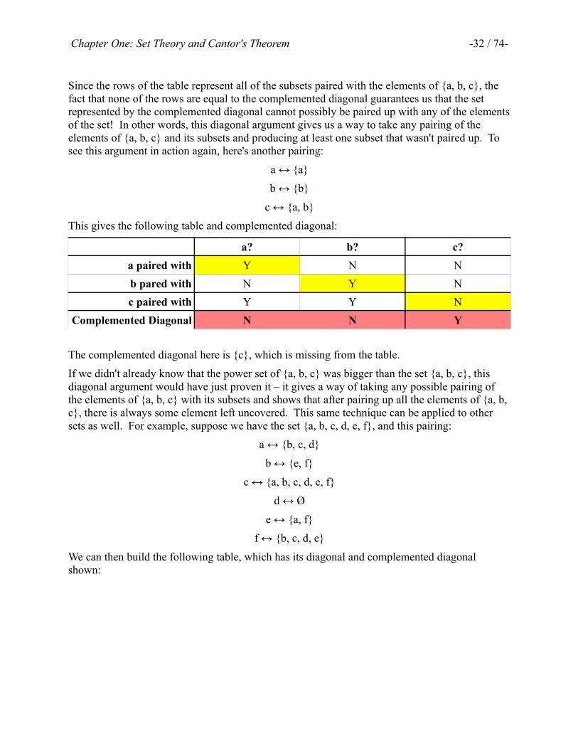
Since the rows of the table represent all of the subsets paired with the elements of {a, b, c}, the fact that none of the rows are equal to the complemented diagonal guarantees us that the set represented by the complemented diagonal cannot possibly be paired up with any of the elements of the set! In other words, this diagonal argument gives us a way to take any pairing of the elements of {a, b, c} and its subsets and producing at least one subset that wasn't paired up. To see this argument in action again, here's another pairing:

a ↔ {a}

b ↔ {b}

c ↔ {a, b}

This gives the following table and complemented diagonal:

a? b? c?

a paired with Y N N

b pared with N Y N

c paired with Y Y N

Complemented Diagonal N N Y

The complemented diagonal here is {c}, which is missing from the table.

If we didn't already know that the power set of {a, b, c} was bigger than the set {a, b, c}, this diagonal argument would have just proven it – it gives a way of taking any possible pairing of the elements of {a, b, c} with its subsets and shows that after pairing up all the elements of {a, b, c}, there is always some element left uncovered. This same technique can be applied to other sets as well. For example, suppose we have the set {a, b, c, d, e, f}, and this pairing:

a ↔ {b, c, d}

b ↔ {e, f}

c ↔ {a, b, c, d, e, f}

d ↔ Ø

e ↔ {a, f}

f ↔ {b, c, d, e}

We can then build the following table, which has its diagonal and complemented diagonal shown:


a? b? c? d? e? f?

a paired with N Y Y Y N N

b pared with N N N N Y Y

c paired with Y Y Y Y Y Y

d paired with N N N N N N

e paired with Y N N N N Y

f paired with N Y Y Y Y N

Complemented Diagonal Y Y N Y Y Y

From this, we get that the complemented diagonal is the set {a, b, d, e, f}, which indeed is not in the list of sets described in the pairing.

Formalizing the Diagonal Argument

We have just described the intuition behind Cantor's diagonal argument – we can show that in any pairing between a set S and the set (℘ S), there must be some element of (℘ S) that isn't covered by the pairing. However, so far our proof requires us to construct a table representing the pairing whose size is determined by the number of elements in S. Given this, will this argument work when we are dealing with infinite sets? We've seen a lot of strange results that appear when working with the infinite, and so it doesn't seem particularly “safe” to assume that this approach, which works in the finite case, scales up to the infinite case.

It turns out, however, that this argument can indeed be applied to infinite sets! However, to do so will require us to be more precise and formal than our reasoning above, in which we just drew a picture. We need to find a way of nicely describing what set is constructed by the diagonal argument without having to draw out a potentially infinite table. Fortunately, there is a nicely straightforward way to do this. Let's consider the previous example:

a ↔ {b, c, d}

b ↔ {e, f}

c ↔ {a, b, c, d, e, f}

d ↔ Ø

e ↔ {a, f}

f ↔ {b, c, d, e}


a? b? c? d? e? f?

a paired with N Y Y Y N N

b pared with N N N N Y Y

c paired with Y Y Y Y Y Y

d paired with N N N N N N

e paired with Y N N N N Y

f paired with N Y Y Y Y N

Complemented Diagonal Y Y N Y Y Y

Now, let's think about the diagonal of this table. Notice that each diagonal entry represents whether some element x ∈ S is paired with a set that contains itself. If the element x is paired with a set that contains it, the the entry on the diagonal is a Y, and if x is paired with a set that doesn't contain it, then the entry on the diagonal is an N. In the complemented diagonal, this is reversed – the complemented diagonal entry is a Y if x is paired with a set that doesn't contain x, and is an N if x is paired with a set that does contain x. In other words, we can think about the set defined by the complemented diagonal (let's call it D) as follows:

D = { x | there is an N in the diagonal entry for x }

Or, more concretely:

D = { x | x is paired with an set that does not contain x }

Now this is interesting – we now have a definition of the diagonal set D that doesn't require us to even construct the table! The rule for finding D is straightforward: we simply find all the elements of the set S that are paired with subsets of S that don't contain themselves, then gather those up together into a set. Does this really work? Well, if experience is a guide, then yes! Here are a few pairings from before, along with the associated diagonal set:

Pairing a ↔ {a}

b ↔ {b}

c ↔ {a, b}

a ↔ {a, b}

b ↔ Ø

c ↔ {a, c}

a ↔ {b, c, d}

b ↔ {e, f}

c ↔ {a, b, c, d, e, f}

d ↔ Ø

e ↔ {a, f}

f ↔ {b, c, d, e}

ComplementedDiagonal Set

{c} {b} {a, b, d, e, f}


You can (and should!) check that in each case, the complemented diagonal set is indeed the set of elements that aren't paired with a set that contains them. For example, in the first example since a is paired with {a} and b is paired with {b}, neither is included in the complemented diagonal set, while c, which is paired with a set that doesn't contain c, is indeed in the complemented diagonal set.

Proving Cantor's Theorem

Given this definition of the diagonal set, we can formally prove Cantor's theorem.

(Cantor's Theorem) For any set S, |S| < | (℘ S)|.

In order to prove Cantor's theorem, let's think about the definition of what it means for one set to have lesser cardinality than another. This would mean that

|S| ≤ | (℘ S)| and |S| ≠ | (℘ S)|

We can prove each part of this independently. Cantor's diagonal argument will handle the second case (which we'll handle in a minute), but first let's show that |S| ≤ | (℘ S)|. How can we show this? To do so, we need to show that we can pair off all of the elements of S with some element in (℘ S). This might seem hard, because we don't actually know what S is; we need to show that for any set S, it's always possible to find such a pairing. This actually ends up being not too difficult. Note that for each element x ∈ S, the set {x} ⊆ S. Therefore, {x} (∈℘ S). Consequently, one way of pairing up all the elements of S with elements from (℘ S) would be to associate each element x ∈ S with the element {x} ∈ (℘ S). This ensures that each element of S is paired up with a unique element from (℘ S).

Now, we need to formally prove that |S| ≠ | (℘ S)|, even though we don't actually know what S is (we're trying to prove the claim for any possible choice of S). So what does it mean for |S| ≠ |

(℘ S)|? Well, this would mean that there must be no possible way of pairing off all the elements from the two sets with one another. How can we show that this is impossible? Here, we will employ a technique called proof by contradiction. In a proof by contradiction, we try to show that some statement P is true by doing the following:

• Assume, hypothetically, that P was false.

• Show that this assumption, coupled with sound reasoning, leads us to a conclusion that is obviously false.

• Conclude, therefore, that our assumption must have been wrong, so P is true.

As an example of a proof of this style, suppose that you want to convince someone that it is not raining outside (if it's raining when you're reading this, then my apologies – please bear with me!) One way to convince someone that it's not raining is as follows:

1. Suppose, hypothetically, that it were raining.

2. Therefore, I should be soaking wet from my walk a few minutes ago.

3. But I am not soaking wet from my walk a few minutes ago.


4. Since steps (2) and (3) are logically sound, the only possible problem is step (1).

5. Conclude, therefore, that it's not raining outside.

Here, when proving that |S| ≠ | (℘ S)|, we will use a proof by contradiction. Suppose, hypothetically, that |S| = | (℘ S)|. Then there is a way of pairing up all of the elements of S an

(℘ S) together – we don't know what it is, but allegedly it exists. This should mean that any element of (℘ S) that we choose should be paired up with some element of S. Since every element of (℘ S) is a subset of S (that's how we defined the power set!), this should mean that if we choose any subset of S, it should be paired up with some element from S. But now we can employ Cantor's diagonal argument. If it's really true that any subset of S must be paired up with some element of S, then surely we should be able to find some element paired up with the set

D = {x | x ∈ S and x is paired with a set that does not x. }

Well, since D allegedly must be paired with something, let's call that element d. But if you'll recall from our discussion of the diagonal argument, we should now be able to show that D actually isn't in this table, meaning that there really isn't an element d that it could be paired with. But how do we show this? Here, we'll simply ask the following question: is d contained in D? There are two possible options: either d ∈D or d ∉D. Let's consider these two cases individually.

First, suppose that d ∈D. Recall that the definition of D says that this means that d would have to be paired with a set that doesn't contain d. Since d is paired with D, this would have to mean that d ∉ D, but this is clearly impossible, because we know that in this case d ∈D. Since if d ∈ D we conclude that d ∉D, we know that it must not be possible for d ∈ D to be true.

So this means that d ∉D. Well, let's see what that means. Since d ∉D, then by looking at the definition of the set D, we can see that this means that the set that d is paired with must contain d. Since d is paired with the set D, this would mean that d ∈ D. But this isn't true!

We have just reached a logical contradiction. If d ∈D, then we know that d ∉D, and similarly if d ∉ D, then d ∈D. In other words, D contains d if and only if D does not contain d. We have reached a logical impossibility.

All of the reasoning we've had up to this point is sound, so we are forced to admit that the only possibility remaining is that our assumption that |S| = | (℘ S)| is incorrect. Consequently, we have proven that |S| ≠ | (℘ S)|. Since earlier we proved |S| ≤ | (℘ S)|, this collectively proves Cantor's theorem.

Why Cantor's Theorem Matters

We have just proven Cantor's theorem, that the number of subsets of a set S is strictly greater than the number of elements of that set S. But why does this matter? It turns out that this is actually a hugely important result with a terrifying corollary. To begin with, note that Cantor's theorem says that there are more subsets of a set than elements of that set, even if the initial set is infinite. This suggests that there is no one concept of “infinity,” and that there are, in fact, different infinitely large quantities, each one infinitely larger than the previous! In fact this means that


• There are more subsets of natural numbers than natural numbers (|ℕ| < | (℘ ℕ)|)

• More subsets of subsets of natural numbers than subsets of natural numbers (| (℘ ℕ)| < |( (℘ ℘ ℕ))|),

• etc.

The fact that there are different infinitely large numbers has enormous significance to the limits of computing. For example, there are infinitely many problems to solve, and there are infinitely many programs to solve them. But this doesn't mean that there are the same number of problems and solutions! In fact, it might be possible that there are more problems that we might want to solve than there are programs to solve them, even though both are infinite! In fact, this is the case. Let's see why.

The Limits of Computation

Let's begin with a pair of definitions:

An alphabet is a set of symbols.

For example, we could talk about the Latin alphabet as the set A = { A, B, C, D, …, Y, Z, a, b, …, z }. The binary alphabet is the alphabet {0, 1}, and the unary alphabet is the alphabet { 1 }. Given an alphabet, what words can we make from that alphabet? The idea of a “word” is captured by this definition:

A string is a finite sequence of symbols drawn from some alphabet.

For example, hello is a string drawn from the Latin alphabet, while 01100001 is a string drawn from the binary alphabet.

Every computer program can be expressed as a string drawn from the appropriate alphabet. The program's source code is a sequence of characters (probably Unicode characters) that are translated into a program using a compiler. In most programming languages, not all strings are legal programs, but many are. As a result, we can say that the number of programs is at most the number of strings, since we can pair up the programs and strings without exhausting all strings (just pair each program with its source code).

Now, let's think about how many problems there are out there that we might want to solve. This really depends on our notion of what a “problem” is, but we don't actually need to have a formal definition of “problem” quite yet. Let's just focus on one type of problem: deciding whether a string has some “property.” For example, some strings have even length, some are palindromes, some are legal C programs, some are mathematical proofs, etc. We can think of a “property” of a string as just a set of strings that happen to share that property. For example, we could say that the property of being a palindrome (reading the same forwards and backwards) could be represented by the set


{ a, b, c, …, z, aa, bb, …, zz, aba, aca, ada, … }

While the property of having exactly four letters would be

{ aaaa, aaab, aaac, …, zzzz }

For each of these properties, we might think about writing a program that could determine whether a string has that given property. For example, with a few minutes' effort you could probably sit down and write a program that will check whether a string is a palindrome or contains just four characters, and with more effort could check if a string encoded a legal computer program, etc. In other words, each property of strings (that is, a set of strings) defines a unique problem – determine whether a given string has that property or not. As a result, the number of sets of strings is no bigger than the total number of problems we might want to solve, since there's at least one problem to solve per set of strings.

This leads to the following line of reasoning:

The number of programs is no bigger than the number of strings.

The number of strings is strictly less than the number of sets of strings (from Cantor's theorem).

The number of problems is at least the number of strings.

Combining this all together gives the following:

The number of programs is strictly less than the number of problems.

In other words:

There are more problems than there are programs to solve them.

We have just proven, without even looking at how computers work or how clever programmers are, that there are problems that cannot possibly be solved by a computer. There are simply too many problems to go around, so even if we wrote all of the infinitely many possible programs, we would not have written a program to solve every problem.

What Does This Mean?

At this point, we could throw up our hands and despair. We have just shown the existence of unsolvable problems, problems that can be formulated but not possibly solved.

Unfortunately, it gets worse. Using more advanced set theory, we can show that the infinity of problems so vastly dwarfs the infinity of solutions that if you choose a totally random problem to solve, the chance that you can is 0. Moreover, since there are more problems to solve than possible strings, some of the problems we can't solve may be so complex that there is no way to describe them; after all, a description is a way of pairing a string with a problem!

But there's no way we can give up now. We have shown that there is an infinite abyss of unsolvable problems, but everywhere we look we can see examples of places where computers have solved problems. Pretty much every aspect of our life has been improved thanks to computers.


Rather than viewing this result as a sign of defeat, treat it as a call to arms. Yes, there are infinitely many problems that we can't solve, but there are infinitely many problems that we can solve as well. What are they? What do they look like? Of the problems we can solve in theory, what can be solved in practice as well? How powerful of a computer would you need to solve them? These are questions of huge practical and theoretical importance, and its these questions that we will focus on in the rest of this book. In doing so, you'll sharpen your mathematical acumen and will learn how to reason about problems abstractly. You'll learn new ways of thinking about computation and how these novel computers can impact your practical programming skills. And you'll see some of the most interesting and fascinating results in all of computer science.

Let's get started!

Chapter Summary

• A set is an unordered collection of distinct elements.

• Sets can be described by listing their elements in some order.

• Sets can also be described using set-builder notation.

• Set can be combined via union, intersection, difference, or symmetric difference.

• Two sets are equal precisely when they have the same elements.

• One set is a subset of another if every element of that set is in the other set.

• The power set of a set is the set of its subsets.

• A statement is vacuously true if its assertion doesn't apply to anything.

• The cardinality of a set is a measure of how many elements are in that set.

• Two sets have the same cardinality if all elements of both sets can be paired up with one another.

• Cantor's diagonal argument can be used to prove Cantor's theorem, that the cardinality of a set is always strictly less than the cardinality of its power set.

Chapter Two: Introduction to Formal Proofs -40 / 74-

Chapter Two: Introduction to Formal ProofsLast chapter we concluded with Cantor's theorem, the fact that the cardinality of the power set of a set S is always greater than the cardinality of the set S itself. Although we worked through a strong argument that this should be true, did we really “prove” it? What does it mean to prove something, at least in a mathematical sense?

Proofs are at the core of the mathematical foundations of computing. Without proofs we couldn't be certain that any of our results were correct, and our definitions would be little better than an intuition to guide us. Accordingly, before we attempt to explore the limits of computation, we first need to build up the machinery necessary to reason about and firmly establish mathematical results.

Proofs are in many ways like programs – they have their own vocabulary, terminology, and structure, and you will need to train yourself to think differently in order to understand and synthesize them. In this chapter and the ones that follow, we will explore proofs and proof techniques, along with several other concepts that will serve as a “proving ground” for testing out these proof ideas.

What is a Proof?

In order to write a proof, we need to start off by coming up with some sort of definition of the word “proof.” Informally, a proof is a series of logical steps starting with one set of assumptions that ends up concluding that some statement must be true. For example, if we wanted to prove the statement

If x + y = 16, then either x ≥ 8 or y ≥ 8

Then we would begin by assuming that x + y = 16, then apply sound logical reasoning until we had arrived at the conclusion that x ≥ 8 or y ≥ 8. Similarly, if we wanted to prove that

For any set S, |S| < | (℘ S)|

(as we started doing last chapter), we would take as our starting point all of the definitions from set theory – what the power set is, what it means for one set to have smaller cardinality than another, etc. - and would proceed through logical steps to conclude that |S| < | (℘ S)|.

Writing a proof is in many ways like writing a computer program. You begin with some base set of things that you know are true (for example, how primitive data types work, how to define classes, etc.), then proceed to use those primitive operations to build up something more complicated. Also like a program, proofs have their own vocabulary, language, structure, and expectations. Unfortunately, unlike programs, there is no “compiler” for proofs that can take in a proof and verify that it's a legal mathematical proof.2 Consequently, learning how to write proofs takes time and effort.

2 Technically speaking such programs exist, but they require the proof to be specified in a very rigid format that is almost never used in formal mathematical proofs.


In this chapter, we will introduce different types of proofs by analyzing real proofs and seeing exactly how they work. We'll also see what doesn't work and the sort of logical traps you can easily fall into when writing proofs.

What Can We Assume?

One of the most difficult aspects of writing a proof is determine what you can assume going into the proof. In journals, proofs often assume that the reader is familiar with important results, and often cite them without reviewing why they're true. For our purposes, though, we will deliberately play dumb and start with a very weak set of assumptions. We will prove pretty much everything we need, even if it seems completely obvious, in order to see how to formalize intuitive concepts with a level of mathematical rigor.

In this book, we will assume that whoever is reading one of our proofs knows

1. All definitions introduced so far,

2. All theorems introduced so far, and

3. Basic algebra.

We will not assume anything more than this. For example, we're fine assuming that if x < y and y < z, then x < z, but we will not assume that for any set S, S ∩ Ø = Ø even though this seems “obvious.” As we build up our mathematical repertoire, the set of assumptions we can make will grow, and it will become easier and easier to prove more elaborate results. This is similar to writing libraries in computer programs – although it's difficult and a bit tedious to implement standard data structures like stacks, queues, and hash tables, once you've put in the work to do so it becomes possible to build up off of them and start writing much more intricate and complex programs.

Direct Proofs

Just as it's often easiest to learn how to program by jumping into the middle of a “Hello, World!” program and seeing how it works, it's useful to jump right into some fully worked-out mathematical proofs to see how to structure general proofs.

To begin our descent into proofs, we'll introduce two simple definitions, then see how to prove results about those definitions.

An integer x is called even if there is some integer k such that x = 2k.

An integer x is called odd if there is some integer k such that x = 2k + 1.

For example, 4 is even since 4 = 2 × 2. 8 is even as well, since 8 = 4 × 2. 9 is odd, because 9 = 4 × 2 + 1. We consider 0 to be an even number, since 0 = 0 × 2.

Given this, let's prove the following result:


If x is even, then x2 is even.

Proof: Let x be any even integer. Since x is even, there is some integer k such that x = 2k. This means that x2 = (2k)2 = 4k2 = 2(2k2). Since 2k2 is an integer, this means that there is some integer m (namely, 2k2) such that x2 = 2m. Thus x2 is even. ■

Let's look at how this proof works. The proof proceeds in several clean logical steps, each of which we can analyze independently.

First, note how the proof starts: “Let x be any even integer.” The goal of this proof is to show that if x is even, then x2 is even as well. This proof should work no matter what choice of x we make – whether it's 0, 2, 4, 6, 8, etc. In order for our proof to work in this general setting, the proof will proceed by using x as a placeholder for whatever even number we're interested in. If we wanted to convince ourselves that some particular even number has a square that's also even, we could just plug that even number into the proof wherever we were using x. For example, if we want to prove that 122 is even, the proof would go like this:

Proof: Since 12 is even, there is some integer k such that 12 = 2k. (This integer k is the integer 6). This means that 122 = (2 × 6)2 = 4 × 62 = 2(2 × 62) = 2 × 72. Since 72 is an integer, this means that there is some integer m (namely, 72) such that 122 = 2m. Thus 122 is even. ■

All that we've done here is substitute in the number 12 for our choice of x. We could substitute in any other even number if we'd like and the proof would still hold. In fact, that's why the proof works – we've shown that no matter what choice of an even number you make for x, you can always prove that x2 is even as well.

Let's continue dissecting this proof. After we've decided to let x be a placeholder for whatever even number we'd like, we then say

Since x is even, there is some integer k such that x = 2k

What does this statement mean? Well, we know that x is an even number, which means that it must be twice some other number. We can't really say what that number is, since we don't know what our choice of x is. However, we can say that there is some number such that x is twice that number. In order to manipulate that number in this proof, we'll give this number a name (in this proof, we call it k). Interestingly, note that nowhere in this sentence do we actually say how to figure out what this value of k is; we just say that it has to exist and move forward. From a programming perspective, this may seem strange – it seems like we'd have to show how to find


this number k in order to assert that it exists! But it turns out that it's perfectly fine to just say that it exists and leave it at that. Our definition of an even number is an integer that is equal to twice some other number, so we know for a fact that because x is even, this number k must exist.

At this point, we know that x = 2k, and our goal is to show that x2 is even. Let's think about how to do this. To show that x2 is even, we will need to find some integer m such that x2 = 2m. Right now, all that we know that is that x is even and, as a result, that x = 2k for some choice of k. Since we don't have much else to go on right now, let's try seeing if we can describe x2 in terms of x and k. Perhaps doing this will lead us to finding some choice of m that we can make such that x2 = 2m. This leads to the next part of the proof:

This means that x2 = (2k)2 = 4k2 = 2(2k2). Since 2k2 is an integer, this means that there is some integer m (namely, 2k2) such that x2 = 2m

The first of these two sentences is a simple algebraic manipulation. We know that x = 2k, so x2 = (2k)2. If we simplify this, we get x2 = 4k2, which is in turn equal to 2(2k2). This last step – factoring out the two from the expression – then makes it clearer that x2 is twice some other integer (specifically, the integer 2k2). We can then conclude that there is some natural number m such that x2 = 2m, since we've found specifically what that value was. Because we've done this, we can conclude the proof by writing:

Thus x2 is even. ■

This holds because the definition of an even number is one that can be written as 2m for some integer m. Notice that we've marked the end of the proof with the special symbol ■, which serves as a marker that we're done. Sometimes you see proofs ended with other statements like “This completes the proof” or “QED” (from the Latin “quod erat demonstrandum,” which translates roughly to “which is what we wanted to show”). Feel free to end your own proofs with one of these three endings.

Let's take a look at an example of another proof:

If m is even and n is odd, then mn is even.

Proof: Let m be any even number and n be any odd number. Then m = 2r for some integer r, and n = 2s + 1 for some integer s. This means that mn = (2r)(2s + 1) = 2(r(2s + 1)). This means that mn = 2k for some integer k (namely, r(2s + 1)), so mn is even. ■


The structure of this proof is similar to the previous proof. We want to show that the claim holds for any choice of even m and odd n, so we begin by letting m and n be any even and odd number, respectively. From there, we use the definition of even and odd numbers to write m = 2r and n as 2s + 1 for some integers r and s. As with the previous proof, we don't actually know what these numbers are, but they're guaranteed to exist. After doing some simple arithmetic, we end up seeing that mn = 2(r(2s + 1)), and since r(2s + 1) is an integer, we can conclude that mn is twice some integer, and so it must be even.

The above proofs are both instances of direct proofs, in which the proposition to be proven is directly shown to be true by beginning with the assumptions and ending at the conclusions.

Proof by Cases

Let's introduce one new definition, which you may be familiar with from your programming background:

The parity of an integer is whether it is odd or even. Two numbers have the same parity if they are both odd or both even.

For example, 1 and 5 have the same parity, because both of the numbers are odd, and 4 and 14 have the same parity because both 4 and 14 are even. However, 1 and 2 have opposite parity, because 1 is odd and 2 is even.

The following result involves the parity of integers:

If m and n have the same parity, then m + n is even.

Before we try to prove this, let's check that it's actually correct by testing it on a few simple examples. We can see that 2 + 6 = 8 is even, and 1 + 5 = 6 is even as well. But how would we prove that this is true in the general case? In a sense, we need to prove two separate claims, since if m and n have the same parity, then either both m and n are even or both m and n are odd. The definitions of odd numbers and even numbers aren't the same, and so we have to consider the two options separately. We can do this cleanly in a proof as follows:


Proof: Let m and n be any two integers with the same parity. Then there are two cases to consider:

Case 1: m and n are even. Then m = 2r for some integer r and n = 2s for some integer s. Therefore, m + n = 2r + 2s = 2(r + s). Thus m + n = 2k for some integer k (namely, r + s), so m + n is even.

Case 2: m and n are odd. Then m = 2r + 1 for some integer r and n = 2s + 1 for some integer s. Therefore, m + n = 2r + 1 + 2s + 1 = 2r + 2s + 2 = 2(r + s + 1). Thus m + n = 2k for some integer k (namely, r + s + 1), so m + n is even. ■

Note how this proof is structured as two cases – first, when m and n are even, and second, when m and n are odd. This style of proof is sometimes called a proof by cases or a proof by exhaustion (because we've exhausted all possibilities and found that the claim is true). Each of the branches of the proof reads just like a normal proof, but is individually insufficient to prove the general result. Only when we show that in both of the possible cases the result holds can we conclude that the claim is true in general.

When writing a proof by exhaustion, it's critically important to remember to check that you have covered all possible cases! If you have a proof where four options are possible and you only prove three cases, your proof is likely to be incorrect.

Let's see another example of a proof by cases:

If n is even and m is an integer, then n + m has the same parity as m.

Before proving this, it's always good to check that it works for a few test cases. If we let n = 4, then we can see that

• 4 + 3 = 7, and 7 has the same parity as 3.

• 4 + 6 = 10, and 10 has the same parity as 6.

Let's see a proof of this result:


Proof: Consider any even integer n. Now, consider any integer m and the sum n + m. We consider two possibilities for m:

Case 1: m is even. Then m and n have the same parity, so by our previous result we know that m + n is even. Therefore m and m + n have the same parity.

Case 2: m is odd. Since n is even, n = 2r for some integer r, and since m is odd, m = 2s + 1 for some integer s. Then n + m = 2r + 2s + 1 = 2(r + s) + 1. This means that n + m = 2k + 1 for some k (namely, r + s), so n + m is odd. Therefore m and m + n have the same parity. ■

This proof is interesting for two reasons. First, notice that in proving that Case 1 is true, we used the result that we have proven previously: if n and m have the same parity, then n + m is even. This means that we didn't have to try writing n = 2r and m = 2s, and we ended up saving a lot of space in our proof. Whenever you're writing a proof, feel free to cite any result that you have previously proven. In CS103, it's perfectly fine to cite proofs from lecture, this book, or the problem sessions, as long as you make it clear what result you're using.

Second, notice that in this proof the cases resulted from the parity of just one of the variables (m). We knew that the parity of n must be even, and the only thing that was unclear was whether m was odd or even.

Proofs about Sets

In the last chapter, we explored sets and some of the operations on them. You have already seen one theorem about sets (specifically, Cantor's theorem). But what else can we prove about sets? And how do we prove them?

Let's begin with a very simple proof about sets:

For any sets A and B, A ∩ B ⊆ A.

This theorem intuitively makes sense. We can think of A ∩ B as the set of things that A and B have in common. In other words, we're filtering down the elements of A by just considering those elements that also happen to be in B. As a result, we should end up with a set that's a subset of the set A. So how do we prove this? As you will see, the proof works similarly to our proof about odd and even numbers: it calls back to the definitions of intersection and subset, then proceeds from there.


Proof: Consider any sets A and B. We want to show that A ∩ B ⊆ A. By the definition of subset, this means that we need to show that for any x ∈ A ∩ B, x ∈ A. So consider any x ∈ A ∩ B. By the definition of intersection, x ∈ A ∩ B means that x ∈ A and x ∈ B. Therefore, if x ∈ A ∩ B, x ∈ A. Since our choice of x was arbitrary, A ∩ B ⊆ A. ■

Let's examine the structure of the proof. We initially wanted to prove that A ∩ B ⊆ A. To do this, we said something to the effect of “okay, I need to prove that A ∩ B ⊆ A. What does this mean?” By using the definition of subset, we were able to determine that we needed to prove that for any choice of x ∈ A ∩ B, it's true that x ∈ A. Again we ask – so what does it mean for x

∈ A ∩ B? Again we call back to the definition: x ∈ A ∩ B means that x ∈ A and x ∈ B. But at this point we're done – we needed to show that any x ∈ A ∩ B also satisfies x ∈ A, but the very definition of A ∩ B guarantees this to us!

This proof illustrates a crucial step in many proofs – if you are unsure about how to proceed, try referring to the definitions of the terms involved. Often this simplification will help you make progress toward the ultimate proof by rewriting complex logic in terms of something similar.

Let's do another simple proof:

For any sets A and B, A ⊆ A ∪ B.

This result says that if we take any collection of things (the set A) and combine it together with any other set of things (forming the set A ∪ B), then the original set is a subset of the resulting set. This seems obvious – after all, if we mix in one set of things with another, that initial set is still present! Of course, it's good to formally establish this, which we do here:

Proof: Consider any sets A and B. We want to show that A ⊆ A ∪ B. To do this, we show that for any x ∈ A, x ∈ A ∪ B as well. By definition, x ∈ A ∪ B if either x ∈ A or x ∈ B. Since we know that x ∈ A, it therefore follows that x ∈ A ∪ B as well. Since our choice of x was arbitrary, this means that A ⊆ A ∪ B. ■

Again, notice the calling back to the definitions. We use the definition of subset to prove A ⊆ A ∪ B by arguing that every x ∈ A also satisfied x ∈ A ∪ B. What does it mean for x ∈ A ∪ B?

Well, the definition of A ∪ B is the set of all x such that either x ∈ A or x ∈ B. From there we can see that we're done – if x ∈ A, then it's also true that x ∈ A or x ∈ B, so it's true that x ∈ A ∪ B.

Let's do another proof, this time proving a slightly more complex result:


For any sets A, B, and C, C – (A ∩ B) (⊆ C – A) (∪ C – B)

First, let's try to make sense of what on earth this says in the first place. What this theorem states is the following: suppose that you have some big set C and two sets A and B. If you remove from C all the elements in A ∩ B (the things in common to A and B), this is equivalent to removing everything in A from C, then removing everything in B from C, and finally combining those two sets together.

We could try to argue intuitively why this would be true, but to be more formal let's try establishing this rigorously. As in the previous case, the way to do this is simply to keep breaking down the definitions until we get to something easier to work with.

Proof: Consider any sets A, B, and C. We want to show thatC – (A ∩ B) (⊆ C – A) (∪ C – B). By definition, this is true if for any x ∈ C – (A ∩ B), we also have that x ∈ (C – A) (∪ C – B). So consider any x ∈ C – (A ∩ B). By the definition of set difference, this means that x ∈ C and x ∉ A ∩ B. Since we know that x ∉ A ∩ B, we know that it is not the case that both x ∈ A and x ∈ B. Consequently, it must be true that either x ∉ A or x ∉ B. We consider these two cases individually:

Case 1: x ∉ A. Since we know that x ∈ C and x ∉ A, we know that x ∈ C – A. By our earlier result, we therefore have that x (∈ C – A) (∪ C – B).

Case 2: x ∉ B. Since we know that x ∈ C and x ∉ B, we know that x ∈ C – B. By our earlier result, we therefore have thatx (∈ C – A) (∪ C – B).

In either case we have that x (∈ C – A) (∪ C – B). Since our choice of x was arbitrary, we have that C – (A ∩ B) (⊆ C – A) (∪ C – B) as required. ■

Notice that in the course of this proof, we ended up referring back to the proof we did above in which we claimed that for any sets A and B, A ⊆ A ∪ B. Using this theorem, we were able to conclude that if x ∈ C – A, then x (∈ C – A) (∪ C – B). This is extremely common in mathematics. We begin with a few simple terms and definitions, then build up progressively more elaborate results from simpler ones. Most major results do not work from first principles, but instead build off of earlier work by combining well-known results and clever insights.


Lemmas

Let's think about the simple result that A ⊆ A ∪ B. In itself, this isn't very surprising. The proof is simple and straightforward, and in the end we don't end up with anything particular complex. However, as you saw above, this simple result can be used as a building block for proving more elaborate results.

A result that is primarily used as a small piece in a larger proof is sometimes called a lemma. Lemmas are distinguished from theorems primarily by how they're used. Some lemmas, such as the pumping lemma (which you'll learn more about later) are actually quite impressive results on their own, but are mostly used a step in more complex proofs. Other lemmas, like the one you just saw, are simple but necessary as a starting point for future work.

When proving results about sets, lemmas like A ⊆ A ∪ B are often useful in simplifying more complex proofs. In fact, many seemingly obvious results about sets are best proven as lemmas so that we can use them later on.

The first lemma that we'll actually treat as such is the following result, which helps us prove that two sets are equal to one another:

For any sets A and B, A = B if and only if A ⊆ B and B ⊆ A.

Note the use of the phrase if and only if in this lemma. The phrase “P if and only if Q” means that whenever P is true, Q is true, and whenever Q is true, P is true. In other words, “P if and only if Q” means that P and Q have the same truth value – either both P and Q are true, or both P and Q are false. The statement “if and only if” is a very strong assertion – it says that any time we'd like to speak about whether P is true or false, we can instead speak of whether Q is true or false.

As long as we're on the subject, you sometimes see the word iff used to mean “if and only if.” This is a term that we'll use throughout this text, as it's widely used in the mathematical world. Consequently, we might rewrite the above lemma as

For any sets A and B, A = B iff A ⊆ B and B ⊆ A.

Now, let's get down to business – what does this lemma say? The above lemma tells us that two sets A and B are equal to one another if and only if (in other words, precisely when) A is a subset of B and vice-versa. Recall that two sets are equal when they have exactly the same elements; it doesn't matter how we describe or construct the sets, just that they have the same elements. The above lemma states that if we want to show that two sets are equal, all we need to do is show that all of the elements of one set are contained in the other and vice-versa.

So how exactly do we go about proving this lemma? So far, all of the proofs that we've seen have taken the form “if P, then Q.” If we want to prove a statement of the form “P iff Q,” then we need to prove two things – first, if P is true, then Q is true; second, if Q is true, then P is true as well. In other words, both P and Q imply one another.


Given this setup, here is one proof of this result:

Proof: We prove both directions of implication. First, we show that, for any sets A and B, if A = B, then A ⊆ B and B ⊆ A. If A = B, consider any x ∈ A. Since A = B, this means that x ∈ B. Since our choice of x was arbitrary, any x ∈ A satisfies x ∈ B, so A ⊆ B. Similarly, consider any x ∈ B, then since A = B, x ∈ A as well. Since our choice of x was arbitrary, any x ∈ B satisfies x ∈ A, so B ⊆ A.

Now, we prove the other direction of implication. Consider any two sets A and B where A ⊆ B and B ⊆ A. We need to prove that A = B. Since A ⊆ B, for any x ∈ A, x ∈ B as well. Since B ⊆ A, for any x ∈ B, x ∈ A as well. Thus every element of A is in B and vice-versa, so the two sets have the same elements. ■

Let's look at the structure of the proof. Notice how this proof is essentially two separate proofs that together prove a larger result; the first half proves that if two sets are equal each is a subset of the other, and the second half proves that if two sets are subsets of one another they are equal. This is because in order to prove the biconditional, we need to prove two independent results, which together combine to prove the biconditional. Within each piece of the proof, notice that the structure is similar to before. We call back to the definitions of subset and set equality in order to reason about how the elements of the sets are related to one another.

Now that we have this lemma, let's go and use it to prove some Fun and Exciting Facts about set equality! Let's begin with a simple result that teaches something about how symmetric difference works:

For any sets A and B, (A ∪ B) – (A ∩ B) = A Δ B.

Intuitively, this says that we can construct the set symmetric difference as follows. First, combine the two sets A and B together into the larger set A ∪ B. Next, take out from that set all of the elements that are in the intersection of A and B. The remaining elements form the set A Δ B.

To prove this result, we can use our lemma from above, which says that two sets are equal iff each is a subset of the other. The structure of our proof will thus be as follows – we'll show that each set is a subset of the other, then will use the previous lemma to conclude the proof.

Let's begin by showing that (A ∪ B) – (A ∩ B) ⊆ A Δ B. Since this acts a stepping stone toward the larger proof, we'll pose it as a lemma.

Lemma 1: (A ∪ B) – (A ∩ B) ⊆ A Δ B.


How might we prove this lemma? To do so, we'll just call back to the definitions of union, intersection, difference, and symmetric difference:

Proof of Lemma 1: We will show that for any x (∈ A ∪ B) – (A ∩ B), x ∈ A Δ B. So consider any x (∈ A ∪ B) – (A ∩ B). This means that x ∈ A ∪ B, but x ∉ A ∩ B. Since x ∈ A ∪ B, we know that x ∈ A or x ∈ B. Since x ∉ A ∩ B, we know that x is not contained in both A and B. We thus have that x is in at least one of A and B, but not both. Consequently, x ∈ A Δ B. Since our choice of x was arbitrary, we therefore have that (A ∪ B) – (A ∩ B) ⊆ A Δ B. ■

The other direction also will be a lemma for the same reasons. Here's the lemma and the proof:

Lemma 2: A Δ B (⊆ A ∪ B) – (A ∩ B)

This proof is a little bit more involved because there are two completely separate cases to consider when dealing with elements of A Δ B. The proof is below:

Proof of Lemma 2: We will show that for any x ∈ A Δ B,x (∈ A ∪ B) – (A ∩ B). Consider any x ∈ A Δ B. Then either x ∈ A andx ∉ B, or x ∈ B and x ∉ A. We consider these cases separately:

Case 1: x ∈ A and x ∉ B. Since x ∈ A, x ∈ A ∪ B. Since x ∉ B, x ∉ A ∩ B. Consequently, x (∈ A ∪ B) – (A ∩ B).

Case 2: x ∈ B and x ∉ A. Since x ∈ B, x ∈ A ∪ B. Since x ∉ A, x ∉ A ∩ B. Consequently, x (∈ A ∪ B) – (A ∩ B).

In either case, x (∈ A ∪ B) – (A ∩ B). Since our choice of x was arbitrary, we have that A Δ B (⊆ A ∪ B) – (A ∩ B). ■

Now that we have these two lemmas, the proof of the general result is surprisingly straightforward:

Proof of Theorem: By Lemma 1, (A ∪ B) – (A ∩ B) ⊆ A Δ B. By Lemma 2, A Δ B (⊆ A ∪ B) – (A ∩ B). Since each set is a subset of the other, by our earlier lemma we have that (A ∪ B) – (A ∩ B) = A Δ B. ■

That's all that we have to show!


Before we move on to show more applications of the lemma, let's take a minute to examine the proof of Lemma 2. I've reprinted it below:

Proof of Lemma 2: We will show that for any x ∈ A Δ B,x (∈ A ∪ B) – (A ∩ B). Consider any x ∈ A Δ B. Then either x ∈ A andx ∉ B, or x ∈ B and x ∉ A. We consider these cases separately:

Case 1: x ∈ A and x ∉ B. Since x ∈ A, x ∈ A ∪ B. Since x ∉ B, x ∉ A ∩ B. Consequently, x (∈ A ∪ B) – (A ∩ B).

Case 2: x ∈ B and x ∉ A. Since x ∈ B, x ∈ A ∪ B. Since x ∉ A, x ∉ A ∩ B. Consequently, x (∈ A ∪ B) – (A ∩ B).

In either case, x (∈ A ∪ B) – (A ∩ B). Since our choice of x was arbitrary, we have that A Δ B (⊆ A ∪ B) – (A ∩ B). ■

Notice the similarity between Case 1 and Case 2. These two cases are virtually identical, except that we've interchanged the role of the sets A and B. If you'll notice, there really isn't anything in the above proof to suggest that set A is somehow “more important” than set B. If we interchange set A and set B, we change the sets (A ∪ B) – (A ∩ B) and A Δ B to the sets (B ∪ A) – (B ∩ A) and B Δ A. But these are exactly the sets we started with! In a sense, because there really isn't an appreciable difference between A and B, it seems silly to have two completely difference cases dealing with which sets x is contained in.

This situation – in which multiple parts of a proof end up being surprisingly similar to one another – is fairly common, and mathematicians have invented some shorthand to address it. Mathematicians often write proofs like this one:

Proof of Lemma 2: We will show that for any x ∈ A Δ B,x (∈ A ∪ B) – (A ∩ B). Consider any x ∈ A Δ B. Then either x ∈ A and x ∉ B, or x ∈ B and x ∉ A. Assume without loss of generality that x ∈ A andx ∉ B. Since x ∈ A, x ∈ A ∪ B. Since x ∉ B, x ∉ A ∩ B. Consequently,x (∈ A ∪ B) – (A ∩ B). Since our choice of x was arbitrary, we have thatA Δ B (⊆ A ∪ B) – (A ∩ B). ■

Notice the use of the phrase “without loss of generality.” This phrase indicates in a proof that there are several different cases that need to be considered, but all of them are identical to one another once we change the names around appropriately. If you are writing a proof where you find multiple cases that seem identical to one another, feel free to use this phrase to write the proof just once. That said, be careful not to claim that you haven't lost generality if the cases are actually different from one another!

As another example of a proof using “without loss of generality,” let's consider the following theorem, which has nothing to do with sets:


If m and n have opposite parity, m + n is odd.

We can check this pretty easily – 3 + 4 = 7, which is odd, 137 + 42 =179, which is odd, etc. How might we prove this? Well, there are two cases to consider – either m is even and n is odd, or m is odd and n is even. But these two cases are pretty much identical to one another, since m + n = n + m and it doesn't really matter whether it's m or n that's odd. Using this, let's write a quick proof of the above result:

Proof: Without loss of generality, assume that m is odd and n is even. Since m is odd, there exists an integer r such that m = 2r + 1. Since n is even, there exists an integer s such that n = 2s. Then m + n = 2r + 1 + 2s = 2(r + s) + 1. Consequently, m + n is odd. ■

This proof is about half as long as it would be otherwise.

Proofs with Vacuous Truths

To see if we can get some more mileage out of our lemma about set equality, let's try proving some more results about sets. Let's consider the following result:

For any sets A and B, if A ⊆ B, then A – B = Ø.

Now, how might we prove this? Right now, the main tool at our disposal for proving two sets are equal is to show that those two sets are subsets of one another. In other words, to prove the above result, we might try proving two lemmas:

Lemma 1: For any sets A and B, if A ⊆ B, then Ø ⊆ A – B.

Lemma 2: For any sets A and B, if A ⊆ B, then A – B Ø.⊆

Okay, let's set out to prove them. Let's begin by trying to prove lemma 1. To do this, we need to show that every element of the empty set is also contained in A – B. But wait a minute – this doesn't make any sense, since there aren't any x Ø! But not to worry. If you'll recall from∈ Chapter 1, we introduced the idea of a vacuous truth, a statement that is true because it doesn't apply to anything. Fortunately, that's exactly what we have right here – there aren't any elements


of the empty set, so it's vacuously true that every element of the empty set is also contained inA – B, regardless of what A and B actually are. After all, it's also true that every element of the empty set is made of fire, that every element of the empty set is also your best friend, etc.

How do we formalize this in a proof? Well, we can just say that it's vacuously true! This is shown here:

Proof of Lemma 1: We need to show that every element x Ø also satisfies∈ x ∈ A – B. But this is vacuously true, as there are no x satisfying x Ø. ■∈

Well, that was surprisingly straightforward. On to the second lemma!

At first glance, this statement doesn't seem to make any sense. There are no elements of the empty set, so how could something be a subset of the empty set? This would only happen if there are no elements in the first set, since if there were some element x ∈ A – B, then it would have to be true that x Ø, which we know to be impossible. This actually gives us a hint about∈ how to approach the problem. We know that we shouldn't be able to find any x ∈ A – B, so one route for proving that A – B Ø is to directly show that the statement “for any ⊆ x ∈ A – B, x Ø”∈ is vacuously true. This is shown below:

Proof of Lemma 2: We need to show that any x ∈ A – B also satisfies x ∈ Ø. Since A ⊆ B, any x ∈ A also satisfies x ∈ B. Now, consider any x ∈ A – B. This means that x ∈ A and x ∉ B. Since x ∈ A, x ∈ B. But this means that x ∈ B and x ∉ B. Consequently, there are no x ∈ A – B, so the claim that any x ∈ A – B also satisfies x Ø is vacuously true. ■∈

Notice the structure of the proof. We begin by using definitions to tease apart what it means for an element to be in A – B, then show that, in fact, no elements can be in this set. We conclude, therefore, that the entire lemma must be vacuously true.

We can use these two lemmas to complete the proof:

Proof of Theorem: Consider any sets A and B such that A ⊆ B. By Lemma 1, we have that Ø ⊆ A – B. By Lemma 2, we have that A – B Ø. Thus by⊆ our earlier lemma, A – B = Ø as required. ■

Arguably, though, this proof is much more complex than it need be. Lemma 1 is trivially simple, and the overall proof just cites what we have shown here. Instead, let's just rewrite the proof without any lemmas at all:


Proof: We will show that for any sets A and B such that A ⊆ B, Ø ⊆ A – B and A – B Ø. To see that Ø ⊆ ⊆ A – B, note that the claim “for any x, x Ø∈ implies x ∈ A – B” is vacuously true, since there are no x Ø. To show that∈ A – B Ø, we need to show that any x A – B also satisfies ⊆ ∈ x Ø. Since∈ A B, any ⊆ x A also satisfies x B. Now, consider any ∈ ∈ x A – B. This∈ means that x A and ∈ x B. Since ∉ x A, ∈ x B. But this means that ∈ x B∈ and x B. Consequently, there are no ∉ x A – B, so the claim that any∈x A – B also satisfies x Ø is vacuously true. Since the two sets are∈ ∈ subsets of one another, A – B = Ø. ■

Indirect Proofs

The proofs that we have done so far have directly shown that a particular statement must be true. We begin with a set of assumptions, then manipulate those assumptions to arrive at a desired conclusion. However, there is an entirely different family of proof techniques called indirect proofs that indirectly prove that some proposition must be true.

This may seem a bit strange at first, but there are many familiar analogs in real life. For example, suppose that you're biking to class and can't remember whether or not you brought your keys with you. You could directly prove whether you have your keys on you by stopping, getting off your bike, and checking your pockets or purse for your keys. But alternatively, you could use the following line of reasoning. Assuming that you lock your bike (which you should!), you couldn't have unlocked your bike in the first place if you didn't have your keys. Since you definitely unlocked your bike – after all, you're riding it! – you must have your keys with you. You didn't explicitly check to see that you have your keys, but you can be confident that you do indeed have them with you.

In this section, we'll build up two indirect proof techniques – proof by contradiction, which shows that a proposition has to be true because it can't be false, and proof by contrapositive, which proves that P implies Q by proving that an entirely different connection holds between P and Q.

Logical Implication

Before we can move on to talk about proofs by contradiction and contrapositive, we need to discuss logical implication. Many of the proofs that we have done so far are proofs of the form

If P, then Q.

For example, we have proven the following:

If x is even, then x2 is even.

If m is even and n is odd, then mn is even.

If m and n have the same parity, then m + n is even.

If n is even and m is an integer, then n + m has the same parity as m.


If A ⊆ B, then A – B = Ø.

In structuring each of these proofs, the general format has been as follows: first, we assume that P is true, then we show that given this assumption Q must be true as well. To understand why this style of proof works in the first place, we need to understand what the statement “If P, then Q” means. Specifically, the statement “If P, then Q” means that any time P is true, Q is true as well. For example, consider the statement

If x ∈ A, then x ∈ A ∪ B.

This statement says that any time that we find that x is contained in the set A, it will also be contained in the set A ∪ B. If x ∉ A, this statement doesn't tell us anything. It's still possible for x ∈ A ∪ B to be true, namely if x ∈ B, but we don't have any guarantees.

Let's try this statement:

If I don't close the windows, the velociraptors will get inside.

This tells us that in the scenario where I don't close the windows, it's true that the velociraptors will get inside. This doesn't say anything at all about what happens if I do close the windows. It still might be possible for the velociraptors to get inside even if I close the windows (perhaps if I left the door open, or if the windows aren't raptorproof).

The general pattern here is that given a statement of the form

If P, then Q.

Only provides information if P is true. If P is true, we can immediately conclude that Q must be true. If P is false, Q could be true and could be false. We don't have any extra information.

An important point to note here is that implication deals purely with how the truth or falsity of P and Q are connected, not whether or not there is a causal link between the two. For example, consider this (silly) statement:

If I will it to be true, 1 + 1 = 2.

Intuitively, this statement is false: 1 + 1 = 2 because of the laws of mathematics, not because I consciously wish that it is! But mathematically, the statement is true. If I want 1 + 1 = 2 to be true, you will indeed find that 1 + 1 = 2. You'll find 1 + 1 = 2 is true regardless of whether or not I want it to be, but it is indeed true that every time I want 1 + 1 = 2 to be true, 1 + 1 = 2 will be true.

Why discuss these (seemingly pedantic) details at all? The reason for this is to make clear what exactly it means for an implication to be true so that we can discuss what it means for an implication to be false. The statement “If P, then Q” is true if whenever we find that P is true, we also find that Q is true. In order for the statement “If P, then Q” to be false, we have to find an example where P is true (meaning that we expect Q to be true as well), but to our surprise found that Q actually is false. For example, if we wanted to disprove the claim

If x + y is even, then x is odd.


we would have to find an example where x + y was even, but x was not odd. For example, we can take x = 2 and y = 2 as a counterexample, since x + y = 4, but x is not odd. However, if we were to take something like x = 3 and y = 2, it would not be a counterexample: 3 + 2 is not even, so the above claim says nothing about what's supposed to happen.

It's important to make this distinction, because it's surprisingly easy to think that you have disproven an implication that's perfectly true. For example, consider the statement

If A ⊆ B, then A – B = Ø

What happens if we take the sets A = {1, 2} and B = {3}? Then the statement A ⊆ B is false, as is the statement A – B = Ø. However, we have not contradicted the above statement! The above statement only tells us something about what happens when A ⊆ B, and since A isn't a subset of B here, the fact that A – B = Ø doesn't matter.

Proof by Contradiction

One of the most powerful tools in any mathematician's toolbox is proof by contradiction. A proof by contradiction is based on the following logical idea: If a statement cannot possibly be false, then it has to be true.

In a proof by contradiction, we prove some proposition P by doing the following:

1. Assume, hypothetically, that P is not true. This is the opposite of what we want to prove, and so we want to show that this assumption couldn't possibly have been correct.

2. Using the assumption that P is false, arrive at a contradiction – a statement that is logically impossible.

3. Conclude that, since our logic was good, the only possible mistake we could have made would be in assuming that P is not true. Therefore, P absolutely must be true.

Let's see an example of this in action. Earlier, we proved the result that if n is even, then n2 must be even as well. It turns out that the converse of this is true as well:

If n2 is even, then n is even.

Empirically, this seems to pan out. 36 is even, and 36 = 62, with 6 even. 0 is even, and 0 = 02, with 0 even as well. But how would we actually prove this? It turns out that this is an excellent use case for a proof by contradiction.

To prove this statement by contradiction, let's assume that it's false, which means that the statement “If n2 is even, then n is even” is incorrect. As we just saw, this would have to mean that n2 is even, but n itself is odd. Is this even possible? The answer is no – if n were odd, then n2 would have to be odd as well. But we're assuming that n2 is even. This is a problem, because assuming that n2 is even but n is odd causes us to conclude that n2 shouldn't have been even in the first place! This contradiction tells us that something has to be wrong here. The only thing


questionable we did was making the assumption that n is odd with n2 even, and so we can conclude that this can never happen. As a result, if n2 is even, then n would have to be even as well.

We can formalize this in a proof as follows:

Proof: By contradiction; assume that n2 is even but that n is odd. Since n is odd, n = 2k + 1 for some integer k. Therefore n2 = (2k + 1)2 = 4k2 + 4k + 1 = 2(2k2 + 2k) + 1. This means that n2 is odd, contradicting the fact that we know that n2 is even. We have reached a contradiction, so our assumption must have been wrong. Therefore, if n2 is even, n must be even. ■

Let's look at this proof in more depth. First, note how it starts off:

By contradiction; assume that n2 is even but that n is odd.

This sets up how we are going to approach the proof. We state explicitly that we are going to attempt a proof by contradiction. We immediately then say what assumption we are going to make. Here, since we want to contradict the statement “If n2 is even, n is even,” we say that the contradiction is that n2 is even, but n is odd.

Once we have set up the proof by contradiction, the remainder of our proof is a quest to show that this assumption has to have been wrong by deriving a contradiction. The middle section of the proof does just that – it arrives at the conclusion that n2 has to be both odd and even at the same time.

Now that we have our contradiction, we can finish the proof by stating that this contradiction means that we're done:

We have reached a contradiction, so our assumption must have been wrong. Therefore, if n2 is even, n must be even. ■

All proofs by contradiction should end this way. Now that you have the contradiction, explain how it means that the initial assumption was wrong, and from there how this proves the overall result.

Proof by contradiction is a powerful tool. We saw this used in Cantor's theorem in the last chapter (though, admittedly, we haven't seen the formal proof yet), and you will see it used later to prove that several specific important problems cannot be solved by a computer. For now, let's build up some other small examples of how this proof technique can be used.

One interesting application of proofs by contradiction is to show that some particular task cannot be accomplished. Consider the following problem:


You have 2,718 balls and five bins. Prove that you cannot distribute all ofthe balls into the bins such that each bin contains an odd number of balls.

This problem seems hard – there are a lot of ways to distribute those balls into the bins, though as you'll see there's no way to do it such that every bin has an odd number of balls in it. How might we show that this task is impossible? Using the idea of a proof by contradiction, let's start off by hypothetically assuming that you can indeed solve this. Could we then show that this solution leads to some sort of contradiction? Indeed we can. Think of it this way – if we have an odd number of balls in the five bins, then the total number of balls placed into those bins would have to be equal to the sum of five odd numbers. What numbers can you make this way? Well, if we add up two odd numbers, we get an even number (because we know that the sum of two numbers with the same parity is even). If we add up two more of the odd numbers, we get another even number. The sum of those two even numbers is even. If we then add in the last odd number to this even number, we get an odd total number of balls. This is extremely suspicious. We know that the total number of balls has to be odd, because we just proved that it has to. At the same time, we know that there are 2,718 balls distributed total. But this would imply that 2,718 is odd, which it most certainly is not! This is a contradiction, so something we did must have been wrong. Specifically, it has to have been our assumption that we can distribute all of the balls such that each bin has an odd number of balls in it. Therefore, there can't be a solution.

This argument is formalized below as a proof:

Proof: By contradiction; assume that there is a way to distribute all 2,718 balls into five bins such that each bin has an odd number of balls in it. Consider any such way of distributing the balls, and let the number of balls in the five bins be a, b, c, d, and e. Write the sum a + b + c + d + e as ((a + b) + (c + d)) + e. Since all five numbers have the same parity, both(a + b) and (c + d) are even. Since (a + b) and (c + d) have the same parity, ((a + b) + (c + d)) must be even. Then, since ((a + b) + (c + d)) is even, the sum ((a + b) + (c + d)) + e must have the same parity as e. Since e is odd, this means that sum of the number of balls in the five bins is odd, contradicting the fact that there are an even number of balls distributed across the bins (2,718). We have reached a contradiction, so our initial assumption must have been wrong and there is no way to distribute 2,718 balls into five bins such that each bin has an odd number of balls. ■

As an aside, I absolutely love this proof. It pulls together our discussion of direct proofs with parities along with proof by contradiction.

Before we move on, though, let's examine the structure of this proof one more time. Note that it has the same shape as the previous proof. We begin by stating that the proof is by contradiction and what that contradiction is. We then derive a contradiction, and conclude by saying that the contradiction proves the original theorem.


Here is yet another example of a classic proof by contradiction. Consider a standard 8 × 8 chessboard:

Now, suppose that we cut off two diagonally opposite corners, as shown here:

Suppose that we want to cover this chessboard with a set of 2 × 1 dominoes. These dominoes can be positioned horizontally or vertically, but never diagonally. Additionally, we cannot stack the dominoes on top of one another. The question is this – is it possible to cover every square on the modified chessboard with dominoes? Interestingly, the answer is no, and it is impossible to do so.

So why is that? Well, let's approach this from the perspective of a proof by contradiction. Suppose, hypothetically, that we can cover the chessboard with dominoes. Since each domino covers two horizontally or vertically adjacent squares, we know for a fact that each domino covers exactly one white square and exactly one black square. Moreover, since no two dominoes can stack atop one another, if we add up the total number of white squares covered by each domino and the total number of black squares covered by each domino, we should get the total number of white and black squares on the chessboard. But this is where we run into trouble. If each domino covers one white square and one black square, then the total number of white squares and black squares covered should have to be the same. Unfortunately, this isn't true. A standard chessboard has the same number of white and black squares. When we removed two opposite corners, we took away two white squares (check the picture above). This means that


there are, in fact, two more black squares than white squares, contradicting the fact that we were supposed to have the same number of white squares and black squares. This means (again!) that our assumption was wrong, and that there must be no solution to this puzzle.

Formalized as a proof, the above argument looks like this:

There is no way to tile an 8 × 8 chessboard missing two opposite corners with dominoes such that no two dominoes overlap and each domino is aligned horizontally or vertically.

Proof: By contradiction; assume that such a tiling exists. Since each domino is aligned horizontally or vertically across two tiles, each domino covers the same number of white and black squares. Since no two dominoes overlap, each square is covered by exactly one domino. Consequently, the number of white squares on the chessboard and the number of black squares on the chessboard should equal the number of dominoes. In turn, this means that the number of white squares and black squares on the chessboard must be equal. But this is impossible – there are 30 white squares and 32 black squares, and 30 ≠ 32. We have reached a contradiction, so our assumption must have been incorrect. Thus there is no solution to the puzzle. ■

Rational and Irrational Numbers

In computer science we commonly work with the natural numbers or integers because our computers are digital. However, the real numbers are quite important in mathematics, and it would be a disservice to them if we didn't spend at least a little time exploring their properties.

To begin with, we should make a distinction between two different types of real numbers – the rational numbers and the irrational numbers. Intuitively, rational numbers are real numbers that can be expressed as the ratio of two integers. For example, any integer is rational, because the integer x is the ratio x / 1. Numbers like 7/4 and 137/42 are also rational. Formally, we define the rational numbers as follows:

A real number r is called rational if there exist integers p and q such that

1. q ≠ 0,2. p / q = r, and3. p and q have no common divisors other than 1 and -1.


Let's take a minute to see what this says. Rule 1 says that q has to be nonzero, which makes sense given that Rule 2 uses it as the denominator of a fraction. Rule 2 says that the ratio of these integers has to be equal to the number r.

Rule 3 may seem a bit odd, but it's critically important. For a number to be rational, it is not enough that we can find a p and q such that p / q = r and q ≠ 0, but there has to be some “simplest” p and q that we can use. This makes sense – after all, even though 2 = 4/2, we could write it in simpler terms as 2 = 2 / 1.

One more definition is in order:

The set { r | r and ∈ℝ r is rational } is the set of all rational numbers. We denote this set .ℚ

From the definition of , it's clear that . However, is it true that = ? That is, is everyℚ ℚ⊆ℝ ℚ ℝ real number rational? It turns out that the answer to this question is “no.” There are many ways to show this using advanced mathematics, but one simple solution is to find an explicit example of an irrational number. It's not all that hard to find an example of an irrational number – numbers like e and π are irrational, for example – but to actually prove that these numbers are irrational is surprisingly difficult. Instead, we'll focus on a simple example of a number known to be irrational: √2 .

Let's go prove the following theorem, which is a beautiful example of a proof by contradiction:

√2 is irrational.

How exactly can we show this? As you might have guessed from where we are right now, this is a good spot for a proof by contradiction. Let's suppose, for the sake of contradiction, that √2 actually is rational. This means that we can find integers p and q such that q ≠ 0, p / q = √2 , and p and q have no common factors other than 1 and -1 (that is, they're the “simplest” such p and q that we can use). What to do next? Well, ultimately our goal is to derive some sort of contradiction. It's going to be hard to contradict that q ≠ 0, since we're using q in a denominator. This means that we should probably try to contradict either that p / q = √2 or that p and q have no common divisors other than 1 and -1. Of these two claims, the second (the claim about divisibility) is a lot stronger – after all, we just need to find one common divisor of p and q that isn't 1 or -1 and we're done. So let's see if we can contradict it.

Let's start off with some simple algebraic manipulations. Since we have that

p / q = √2

this means that

p2 / q2 = 2

If we then multiply both sides by 2, we get


p2 = 2q2.

What does this tell us? For one thing, we know that p2 has to be an even number, since q2 is an integer and p2 is twice q2. But if you'll recall, one of the first proofs we did by contradiction was the proof that if n2 is even, then n must be even as well. Since p2 is even, this means that p has to be even as well. This tells us that p = 2k for some integer k.

We've just shown that if p / q = √2 , then p has to be even. What can we do with this fact? Well, if we look above, we've shown that p2 = 2q2. What happens if we plug in 2k in place of p? This gives us

(2k)2 = 2q2

4k2 = 2q2

2k2 = q2

This last line tells us that q2 has to be even as well, since it's twice k2 and k2 is an integer. It's at this point that we can see that something unusual is up. Using our previous result, since q2 is even, q has to be even as well. But then both p and q are even, which means that they have to be divisible by two – contradicting the fact that p and q can't have any divisors other than 1 and -1!

In short, our proof worked as follows. Starting with p / q = √2 , we showed that p had to be even. Since p was even, q had to be even as well, meaning that p and q weren't simplified as far as possible. In fact, there's no possible way for them to be simplified – we've shown that whatever choice of p and q you make, they can always be simplified further. This contradicts Rule 3 of rational numbers, and so √2 has to be irrational.

This logic is formalized here in this proof:

Proof:By contradiction; assume that √2 is rational. Then there exists integers p and q such that q ≠ 0, p / q = √2 , and p and q have no common divisors other than 1 and -1.

Since p / q = √2 , this means that p2 / q2 = 2, which means that p2 = 2q2. This means that p2 is even, so by our earlier result p must be even as well. Consequently, there exists some integer k such that p = 2k.

Since p = 2k, we have that 2q2 = p2 = (2k)2 = 4k2, so q2 = 2k2. This means that q2 is even, so by our earlier result q must be even as well. But this is impossible, because it means that p and q have 2 as a common divisor, contradicting the fact that p and q have no common divisors other than 1 and -1.

We have reached a contradiction, so our assumption must have been incorrect. Thus √2 is irrational. ■


Proof by Contrapositive

There is one final indirect proof technique that we will address right now – proof by contrapositive.

To motivate a proof by contrapositive, let's return to our discussion of mathematical implication. Consider the following statement:

If I close the windows, the velociraptors can't get inside.

This statement says that whenever we know that the windows are closed, we know that the velociraptors won't be able to get inside. Now, let's suppose that we know that, unfortunately, the velociraptors did indeed get inside. What could we conclude from this? We know that I certainly didn't close the windows – if I had closed the window, then the raptors wouldn't be inside in the first place!

Let's try another example. Suppose that we know that

If A ⊆ B, then A – B = Ø.

Suppose we find two sets A and B such that A – B ≠ Ø. What can we conclude? Here, we can say that A is not a subset of B, because if it were, then A – B would have been equal to Ø.

There seems to be a pattern here. It seems like if we know that the statement “If P, then Q” is true and we know that Q is false, then we know that P must be false as well. In fact, that's exactly correct. Intuitively, the rationale is that if P implies Q and Q is false, P couldn't be true, because otherwise Q would be true. Given any implication “If P, then Q,” its contrapositive is the statement “If not Q, then not P.” The contrapositive represents the above idea that if Q is false, P has to be false as well.

It's getting a bit tricky to use phrases like “If P, then Q” repeatedly through this text, so let's introduce a bit of notation. We will use the notation P → Q to mean that P implies Q; that is, if P, then Q. Given an implication P → Q, the contrapositive is not Q → not P.

The contrapositive is immensely useful because of the following result:

If not Q → not P, then P → Q.

This theorem is very different from the sorts of proofs that we've done before in that we are proving a result about logic itself! That is, we're proving that if one implication holds, some other implication must hold as well! How might we go about proving this? Right now, we have two techniques at our disposal – we can proceed by a direct proof, or by contradiction. The logic we used above to justify the contrapositive in the first place was reminiscent of a proof by contradiction (“well, if Q is false, then P couldn't be true, since otherwise Q would have been true.”). Accordingly, let's try to prove this by contradiction.

How might we do this? First, let's think about the contradiction of the above statement. Since we are contradicting an implication, we would assume that not Q → not P, but that P → Q is false. In turn we would ask: what does it mean for P → Q to be false? This would only be possible if P was true but Q was not. So at this point, we know the following:


1. not Q → not P.

2. P is true.

3. Q is false.

And now all of the pieces fall into place. Since Q is false, we know that not Q is true. Since not Q implies not P, this means that not P is true, which in turn tells us that P should be false. But this contradicts the fact that P is true. We've hit our contradiction, and can conclude, therefore, that if not Q → not P, then P → Q.

Here is a formal proof of the above:

Proof: By contradiction; assume that not Q → not P, but that P → Q is false. Since P → Q is false, we know that P is true but Q is false. Since Q is false and not Q → not P, we have that P must be false. But this contradicts the fact that we know that P is true. We have reached a contradiction, so our initial assumption must have been false. Thus ifnot Q → not P, then P → Q. ■

This proof has enormous importance for how we can prove implications. If we want to prove that P → Q, we can always instead prove that not Q → not P. This then implies P → Q is true.

Let's work through an example of this. Earlier we proved the following result:

If n2 is even, then n is even.

Our proof proceeded by contradiction. What if we wanted to prove this result by contrapositive? Well, we want to show that if n2 is even, then n is even. The contrapositive of this statement is that if n is not even, then n2 is not even. More clearly, if n is odd, then n2 is odd. If we can prove that this statement is true, then we will have successfully proven that if n2 is even, then n is even. Such a proof is shown here:

Proof: By contrapositive; we prove that if n is odd, then n2 is odd. Let n be any odd integer. Since n is odd, n = 2k + 1 for some integer k. Therefore,n2 = (2k + 1)2 = 4k2 + 4k + 1 = 2(2k2 + 2k) + 1. Thus n2 is odd. ■

Notice the structure of the proof. As with a proof by contradiction, we begin by announcing that we're going to use a proof by contradiction. We then state the contrapositive of the statement that we want to prove, both so that readers know what to expect and so that we're clear on what we want to show. From there, we proceed just as we would in a normal proof – we need to show that if n is odd, n2 is odd, and so we assume that n is odd and proceed from there. The result is a remarkably clean and elegant proof.


Here's another example of a proof by contrapositive: suppose that we have 16 objects that we want to distribute into two bins. There are many ways that we might do this – we might split them evenly as an 8/8 split, or might put all of them into one bin to give a 16/0 split, or might have something only a bit lopsided, like a 10/6 split. Interestingly, though, notice that in each case we have at least one bin with at least 8 objects in it. Is this guaranteed to happen? Or is it just a coincidence?

It turns out that this isn't a coincidence, and in fact we can prove the following:

If m + n = 16, then m ≥ 8 or n ≥ 8.

To prove this by contrapositive, we first need to figure out what the contrapositive of the above statement is. Right now, we have the following:

m + n = 16 → m ≥ 8 or n ≥ 8

The contrapositive of this statement is

not (m ≥ 8 or n ≥ 8) → not (m + n = 16)

Hmmm... that's not very easy to read. Perhaps we can simplify it. Let's start with the right-hand side. We can simplify not (m + n = 16) to the easier m + n ≠ 16. This gives

not (m ≥ 8 or n ≥ 8) → m + n ≠ 16

But what about the first part? This is a bit more subtle. What is the opposite of m ≥ 8 or n ≥ 8? Well, this statement is true if either m ≥ 8 or n ≥ 8, so for it to be false we need to ensure that both m ≥ 8 and n ≥ 8 are false. This would be true if m < 8 and n < 8. This gives us the final contrapositive of

m < 8 and n < 8 → m + n ≠ 16

The important takeaway point from this process is as follows – when determining the contrapositive of a statement, be very careful to make sure that you understand how to negate things properly!

From here, the reason why the initial statement is true should be a bit clearer. Essentially, if both m and n are too small, then their sum can't be 16. This is formalized below:

Proof: By contrapositive; we show that if m < 8 and n < 8, then m + n ≠ 16. To see this, note that m + n < 8 + n < 8 + 8 = 16, so m + n < 16. Consequently, m + n ≠ 16. ■

Chapter Three: Graphs, Functions, and Relations -67 / 74-

Chapter Three: Graphs, Functions, and RelationsGeneral sketch:

• Basic terms and definitions:

• Cartesian product

• Graphs

• Basic terms and definitions

• Examples in practice

• DAGs and topological sorting

• Relations

• Basic terms and definitions

• Reflexivity

• Symmetry

• Transitivity

• Equivalence Relations

• Antisymmetry

• Partial Orders

• Total Orders

• Irreflexivity

• Strict Orders

• Composition

• Closure

• Inverse

• Functions

• Definitions

• Defining Functions

• Injective

• Surjective

• Bijective

• Cardinalities II

Chapter Three: Graphs, Functions, and Relations -68 / 74-

• Cantor's Theorem II

• Inverses

Chapter Four: The Pigeonhole Principle -69 / 74-

Chapter Four: The Pigeonhole PrincipleGeneral sketch:

• Simple counting arguments

• Statement of the principle

• Examples

• Generalized pigeonhole principle

• Examples

• Limits of data compression

Chapter Five: Mathematical Induction -70 / 74-

Chapter Five: Mathematical InductionGeneral idea:

• Definitions

• Basic examples

• Terminology

• Structuring proofs by induction

• Examples:

• Summations

• Balancing games

• Tilings

• Strong induction

• More examples

• More games

• Well-Ordering Principle

• Definition

• Examples

Chapter Six: Proofs about Programs -71 / 74-

Chapter Six: Proofs about ProgramsGeneral Outline:

• Proving properties of loops

• Initialization

• Maintenance

• Termination

• Simple Fibonacci code

• Simple adding code

• Monoids

• Binary search

• Strict total orders

• Sorting algorithms

• Strict total orders

• Counting sort

• Radix sort

Chapter Seven: Formal Logic -72 / 74-

Chapter Seven: Formal LogicGeneral outline:

• Why logic?

• Propositional logic

• FOL


Alphabetical Indexalphabet..........................................................................................................................................37axiom of extensionality..................................................................................................................16Cantor's Diagonal Argument..........................................................................................................30Cantor's Theorem...........................................................................................................................35cardinality......................................................................................................................................21contradiction..................................................................................................................................57contrapositive.................................................................................................................................64direct proof.....................................................................................................................................44element.............................................................................................................................................4empty set..........................................................................................................................................6even................................................................................................................................................41finite set..........................................................................................................................................12Galileo Galilei................................................................................................................................23Georg Cantor...............................................................................................................................22p.if and only if...................................................................................................................................49iff....................................................................................................................................................49implication.....................................................................................................................................64indirect proof..................................................................................................................................55infinite set.......................................................................................................................................12intersection.......................................................................................................................................7irrational number............................................................................................................................61lemma.............................................................................................................................................49logical implication.........................................................................................................................55natural number...............................................................................................................................11Ø.......................................................................................................................................................6odd..................................................................................................................................................41parity..............................................................................................................................................44power set........................................................................................................................................20proof by cases................................................................................................................................45proof by contradiction..............................................................................................................35, 57proof by contrapositive..................................................................................................................64proof by exhaustion........................................................................................................................45QED...............................................................................................................................................43rational number..............................................................................................................................61set.....................................................................................................................................................4set difference....................................................................................................................................9set of all integers............................................................................................................................10set of all natural numbers...............................................................................................................11set of all rational numbers..............................................................................................................62set of all real numbers....................................................................................................................12set of positive natural numbers......................................................................................................12set symmetric difference................................................................................................................10set-builder notation........................................................................................................................12


strict subset.....................................................................................................................................17strict superset.................................................................................................................................17subset..............................................................................................................................................16union................................................................................................................................................8vacuous truth............................................................................................................................18, 53Venn diagram...................................................................................................................................7without loss of generality...............................................................................................................52→....................................................................................................................................................64∈.......................................................................................................................................................4∉.......................................................................................................................................................4⊂....................................................................................................................................................17⊃....................................................................................................................................................17⊆....................................................................................................................................................16⊇....................................................................................................................................................16■.....................................................................................................................................................43ℕ....................................................................................................................................................11ℕ⁺..................................................................................................................................................12ℝ....................................................................................................................................................12ℤ.....................................................................................................................................................10ℵ₀....................................................................................................................................................22

Documents

Mathematical Foundations of Computing - Stanford Universityweb.stanford.edu/class/archive/cs/cs103/cs103.1126... · Mathematical Foundations of Computing-1 / 74-Mathematical Foundations