Embed Size (px)
Citation preview
Masterstudiengang Biologie
MASTERARBEIT
Acoustic presence of marine mammals in the Southern Ocean in 2013.
An observation of vocal presence based on year-round passive acoustic monitoring data.
vorgelegt von
Karoline Hots
Betreuende Gutachterinnen:
Prof. Dr. Gabriele Gerlach
Institut für Biologie und Umweltwissenschaf-
ten, Carl von Ossietzky University Oldenburg
Dr. Ilse van Opzeeland
Ocean Acoustics Lab, Physical Oceanography
of the Polar Seas, Alfred-Wegener-Institut
Helmholtz-Zentrum für Polar- und Meeresfor-
schung, Bremerhaven
Externe Betreuerin:
Dr. Irene Torrecilla Roca
Helmholtz Institut für Funktionelle Marine Bi-
ologie, Oldenburg
Oldenburg, 01.11. 2019
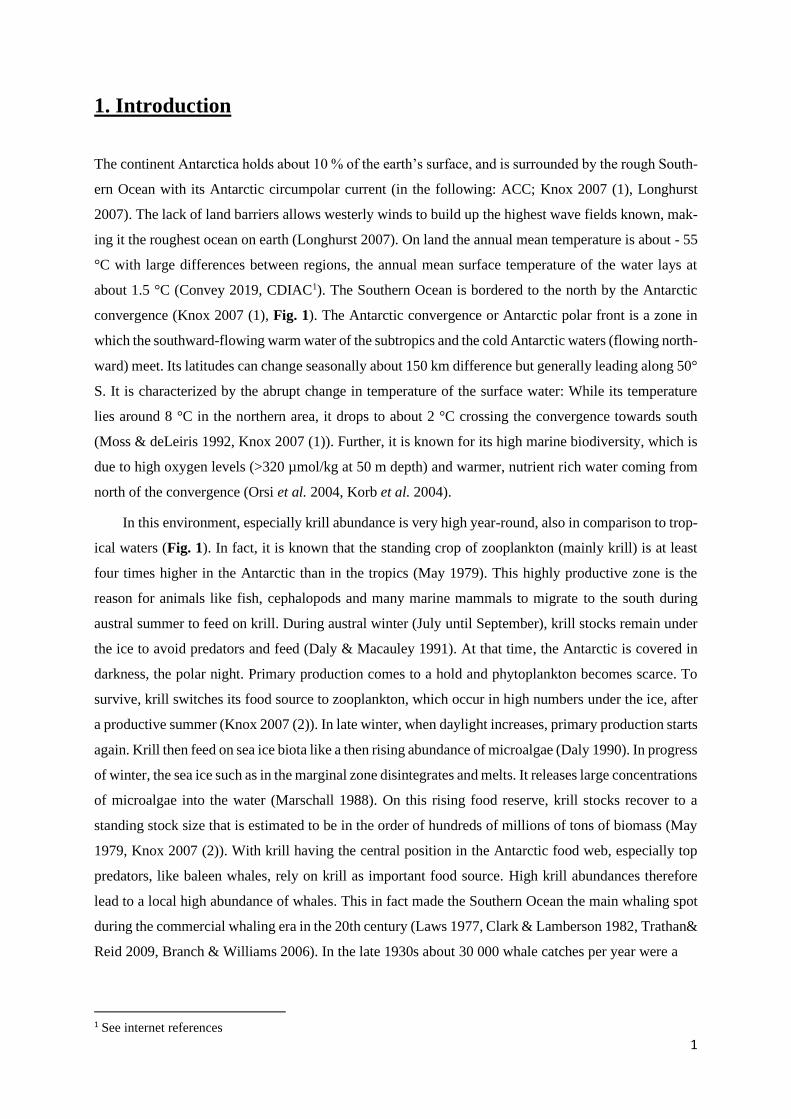
© Paul Nicklen

Acoustic presence of marine mammals in
the Southern Ocean in 2013.
An observation of vocal presence based on year-round
passive acoustic monitoring data.


Table of contents
Abstract .................................................................................................................................................. 8
1. Introduction ....................................................................................................................................... 1
2. Material and Methods ....................................................................................................................... 4
2.1 Passive acoustic data acquisition ................................................................................................... 4
2.2 Subsampling scheme ..................................................................................................................... 5
2.3 Data analysis.................................................................................................................................. 6
2.3.1 Recordings .............................................................................................................................. 6
2.3.2 Ice data ................................................................................................................................... 6
2.3.3 Biodiversity Indices ................................................................................................................ 8
3. Results ................................................................................................................................................ 8
3.1 Detected sounds ........................................................................................................................... 10
3.1.1 Baleen whales ....................................................................................................................... 10
3.1.2 Toothed whales ..................................................................................................................... 18
3.1.3 Seals...................................................................................................................................... 19
3.1.4 Other sounds ......................................................................................................................... 22
3.2 Species acoustic appearance over time ........................................................................................ 25
3.2.1. Seasonal patterns ................................................................................................................. 25
3.2.1.1 Baleen whales .................................................................................................................... 27
3.2.1.2 Toothed whales .................................................................................................................. 28
3.2.1.3 Seals................................................................................................................................... 28
3.2.2 Hourly patterns ..................................................................................................................... 29
3.3 Ice concentration ......................................................................................................................... 31
3.3.1 Baleen whales ....................................................................................................................... 32
3.3.2 Toothed whales ..................................................................................................................... 33
3.3.3 Seals...................................................................................................................................... 33
3.4 Correlations/Biodiversity indices ................................................................................................ 35
3.4.1 Species co-occurrence .......................................................................................................... 35
3.4.2 Acoustic indices ................................................................................................................... 35
4. Discussion ......................................................................................................................................... 37
4.1 Baleen whales .............................................................................................................................. 37
4.1.1 Migratory behavior ............................................................................................................... 37
4.1.2 Hourly patterns ..................................................................................................................... 39
4.1.2 Antarctic blue whales ........................................................................................................... 40
4.1.3 Fin whales ............................................................................................................................. 41
4.1.4 Humpback whales ................................................................................................................ 42
4.1.5 Antarctic minke whales ........................................................................................................ 44
4.2 Toothed whales ............................................................................................................................ 45
4.2.1 Killer whales ......................................................................................................................... 46
4.2.2 Sperm whales ....................................................................................................................... 47
4.3 Seals ............................................................................................................................................ 48
4.3.1 Seasonal behavior ................................................................................................................. 48
4.3.2 Ross seals ............................................................................................................................. 49
4.3.3 Weddell seals ........................................................................................................................ 50
4.4 Other sounds ................................................................................................................................ 51
4.4.1 Unidentified toothed whale .................................................................................................. 51
4.4.2 “February –Fish” .................................................................................................................. 51
4.4.3 Mechanical sound ................................................................................................................. 52
4.4.4 RAFOS ................................................................................................................................. 52
4.5 Correlations/Biodiversity Indices ................................................................................................ 52
4.5.1 Correlation for co-occurring species .................................................................................... 52
4.5.2 Biodiversity indices .............................................................................................................. 54
5. Conclusion ........................................................................................................................................ 55
References ............................................................................................................................................ 56
Internet References ............................................................................................................................. 72
Appendix ................................................................................................................................................. i
Appendix A: General information on analyzed data ............................................................................ i
Appendix B: Ice concentration ............................................................................................................ ii
Appendix C: Subsampling Scheme .................................................................................................... iv
Appendix D: Tables to different vocal activities ................................................................................ vi
Appendix E: Monthly acoustic presence of all species and toothed whales ..................................... vii
Appendix F: Daily appearance of detected Antarctic marine mammals. ......................................... viii
Appendix G: Vocal activity of marine mammals ............................................................................... xi
Appendix H: Missing hourly patterns for fin and sperm whales and Ross seals ............................. xiv
Appendix I: Killer whale ecotypes .................................................................................................... xv
Appendix J: Several killer and humpback whales vocalizing at the same time ............................... xvi
Acknowledgements .................................................................................................................................. i
Abstract
Over decades, various whale species suffered from commercial whaling in the Southern Ocean and are
still not recovered. Many of them still categorized as “threatened”, “near threatened” or “endangered”.
Furthermore, these days man-induced climate change poses the biggest threat to the survival of marine
mammals in the Southern Ocean. Especially ice-breeding seals are expected to be strongly effected.
Hence, there is a desperate need to collect data on marine mammals, to observe the effects of such
catastrophes and their ongoing development to make sustainable management decisions. Beside visual
surveys, passive acoustic monitoring (PAM) is getting more and more popular to collect long-term data
cost and time efficiently, especially in inhospitable regions such as the Southern Ocean during austral
winter. Collected acoustic data give the opportunity to observe the presence of vocalizing marine mam-
mals year-round and to associate it with a behavioral context. This study deals with PAM data recorded
in the Weddell Sea over 10 months in 2013. The data enabled to detect nine marine mammal species:
Four baleen and two toothed whale species and three seal species. Three of the four baleen whale spe-
cies, known to by migratory, were detected year-round. For two species, song, used in a mating context,
was recorded year-round. Further, the seasonal cycle of ice-breeding Antarctic seal species was noticed.
Results reveal that marine mammals frequent the observed area to feed, breed and mate throughout the
whole year, showing its importance and need to be protected. Beside the analysis ot PAM data, biodi-
versity indices were applied to my hand-browsed data, but yield to no reliable results.
Zusammenfassung
Über Jahrzehnte hinweg litten viele Walarten unter dem kommerziellem Walfang im Südpolarmeer und
haben sich größtenteils bis heute nicht erholt. Viele von ihnen sind immer noch als "bedroht", "fast
bedroht" oder "gefährdet" eingestuft. Darüber hinaus ist der vom Menschen verursachte Klimawandel
heutzutage die größte Bedrohung für das Überleben von Meeressäugern im Südpolarmeer. Es wird da-
von ausgegangen, dass im Besonderen antarktische Robben, die auf verschieden Weise auf Eis ange-
wiesen sind, stark betroffen sein werden. Es besteht daher ein dringender Bedarf, Daten über antarkti-
sche Meeressäuger zu sammeln, um die Auswirkungen solcher Katastrophen und deren weitere Ent-
wicklung zu beobachten und Entscheidungen für einen nachhaltigen Tier- und Naturschutz zu treffen.
Neben visuellen Erfassungen gewinnt das passive akustische Monitoring (PAM) immer mehr an Bedeu-
tung, um Langzeitdaten kosten- und zeiteffizient zu erfassen, insbesondere in unwirtlichen Regionen
wie dem Südpolarmeer im südlichen Winter. Gesammelte akustische Daten geben die Möglichkeit, das
Vorhandensein vokalisierender Meeressäuger das ganze Jahr über zu beobachten und mit ihrem Verhal-
ten in Verbindung zu bringen. Diese Studie befasst sich mit PAM-Daten, die 2013 über 10 Monate im

Weddellmeer aufgezeichnet wurden. Die Daten ermöglichten den Nachweis von neun Meeressäugerar-
ten: Vier Barten- und zwei Zahnwalarten, sowie drei Robbenarten. Drei der vier Bartenwalarten, die als
Zugwale bekannt sind, wurden das ganze Jahr über nachgewiesen. Für zwei Arten wurde typisches Sin-
gen, das in einem Paarungskontext verwendet wird, das ganze Jahr über aufgezeichnet. Ferner wurde
der saisonale Zyklus antarktischer Robbenarten festgestellt. Die Ergebnisse zeigen, dass Meeressäuger
das ganze Jahr über das beobachtete Gebiet auf der Suche nach Nahrung, zur Aufzucht und Paaren
aufsuchen. Dies zeigt, wie wichtig und schützenswert dieses Gebiet für frequentierendes Meeressäuger
ist. Neben der Analyse von PAM-Daten wurden Biodiversitätsindizes auf meine analysierten Daten an-
gewendet, die jedoch keine verlässlichen Ergebnisse lieferten.
1
1. Introduction
The continent Antarctica holds about 10 % of the earth’s surface, and is surrounded by the rough South-
ern Ocean with its Antarctic circumpolar current (in the following: ACC; Knox 2007 (1), Longhurst
2007). The lack of land barriers allows westerly winds to build up the highest wave fields known, mak-
ing it the roughest ocean on earth (Longhurst 2007). On land the annual mean temperature is about - 55
°C with large differences between regions, the annual mean surface temperature of the water lays at
about 1.5 °C (Convey 2019, CDIAC1). The Southern Ocean is bordered to the north by the Antarctic
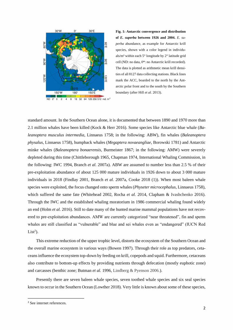
convergence (Knox 2007 (1), Fig. 1). The Antarctic convergence or Antarctic polar front is a zone in
which the southward-flowing warm water of the subtropics and the cold Antarctic waters (flowing north-
ward) meet. Its latitudes can change seasonally about 150 km difference but generally leading along 50°
S. It is characterized by the abrupt change in temperature of the surface water: While its temperature
lies around 8 °C in the northern area, it drops to about 2 °C crossing the convergence towards south
(Moss & deLeiris 1992, Knox 2007 (1)). Further, it is known for its high marine biodiversity, which is
due to high oxygen levels (>320 µmol/kg at 50 m depth) and warmer, nutrient rich water coming from
north of the convergence (Orsi et al. 2004, Korb et al. 2004).
In this environment, especially krill abundance is very high year-round, also in comparison to trop-
ical waters (Fig. 1). In fact, it is known that the standing crop of zooplankton (mainly krill) is at least
four times higher in the Antarctic than in the tropics (May 1979). This highly productive zone is the
reason for animals like fish, cephalopods and many marine mammals to migrate to the south during
austral summer to feed on krill. During austral winter (July until September), krill stocks remain under
the ice to avoid predators and feed (Daly & Macauley 1991). At that time, the Antarctic is covered in
darkness, the polar night. Primary production comes to a hold and phytoplankton becomes scarce. To
survive, krill switches its food source to zooplankton, which occur in high numbers under the ice, after
a productive summer (Knox 2007 (2)). In late winter, when daylight increases, primary production starts
again. Krill then feed on sea ice biota like a then rising abundance of microalgae (Daly 1990). In progress
of winter, the sea ice such as in the marginal zone disintegrates and melts. It releases large concentrations
of microalgae into the water (Marschall 1988). On this rising food reserve, krill stocks recover to a
standing stock size that is estimated to be in the order of hundreds of millions of tons of biomass (May
1979, Knox 2007 (2)). With krill having the central position in the Antarctic food web, especially top
predators, like baleen whales, rely on krill as important food source. High krill abundances therefore
lead to a local high abundance of whales. This in fact made the Southern Ocean the main whaling spot
during the commercial whaling era in the 20th century (Laws 1977, Clark & Lamberson 1982, Trathan&
Reid 2009, Branch & Williams 2006). In the late 1930s about 30 000 whale catches per year were a
1 See internet references
2
standard amount. In the Southern Ocean alone, it is documented that between 1890 and 1970 more than
2.1 million whales have been killed (Kock & Herr 2016). Some species like Antarctic blue whale (Ba-
leanoptera musculus intermedia, Linnaeus 1758; in the following: ABW), fin whales (Baleanoptera
physalus, Linnaeus 1758), humpback whales (Megaptera novaeangliae, Borowski 1781) and Antarctic
minke whales (Baleanoptera bonaerensis, Burmeister 1867; in the following: AMW) were severely
depleted during this time (Chittleborough 1965, Chapman 1974, International Whaling Commission, in
the following: IWC 1994, Branch et al. 2007a). ABW are assumed to number less than 2.5 % of their
pre-exploitation abundance of about 125 000 mature individuals in 1926 down to about 3 000 mature
individuals in 2018 (Findlay 2001, Branch et al. 2007a, Cooke 2018 (1)). When most baleen whale
species were exploited, the focus changed onto sperm whales (Physeter microcephalus, Linnaeus 1758),
which suffered the same fate (Whitehead 2002, Rocha et al. 2014, Clapham & Ivashchenko 2016).
Through the IWC and the established whaling moratorium in 1986 commercial whaling found widely
an end (Holm et al. 2016). Still to date many of the hunted marine mammal populations have not recov-
ered to pre-exploitation abundances. AMW are currently categorized “near threatened”, fin and sperm
whales are still classified as “vulnerable” and blue and sei whales even as “endangered” (IUCN Red
List2).
This extreme reduction of the upper trophic level, distorts the ecosystem of the Southern Ocean and
the overall marine ecosystem in various ways (Bowen 1997). Through their role as top predators, ceta-
ceans influence the ecosystem top-down by feeding on krill, copepods and squid. Furthermore, cetaceans
also contribute to bottom-up effects by providing nutrients through defecation (mostly euphotic zone)
and carcasses (benthic zone; Butman et al. 1996, Lindberg & Pyenson 2006.).
Presently there are seven baleen whale species, seven toothed whale species and six seal species
known to occur in the Southern Ocean (Lowther 2018). Very little is known about some of these species,
2 See internet references.
Fig. 1: Antarctic convergence and distribution
of E. superba between 1926 and 2004. E. su-
perba abundance, as example for Antarctic krill
species, shown with a color legend in individu-
als/m² within each 5° longitude by 2° latitude grid
cell (ND: no data, 0*: no Antarctic krill recorded).
The data is plotted as arithmetic mean krill densi-
ties of all 8127 data collecting stations. Black lines
mark the ACC, boarded to the north by the Ant-
arctic polar front and to the south by the Southern
boundary (after Hill et al. 2013).
3
like AMW or many seal species (e.g. Van Opzeeland et al. 2010, Hückstädt 2015 (1), Cooke et al. 2018).
In the past, most surveys, which observed the Antarctic biodiversity and the behavior of certain species,
were conducted visually. These observations are mostly limited to late austral spring, due to insufficient
light or rough weather conditions (e.g. Secchi et al. 2001, Thiele et al. 2004, Friedlaender et al. 2006).
Unfortunately, possibilities to observe species’ behavior are therefore limited to a short period during
the year, leaving knowledge gaps such as winter data, annual trends, community composition and be-
havior throughout different seasons. Still, marine mammal sighting data provide important insights, such
as species’ distribution, number of individuals, behavior, sex ratios or age. However, low encounter
rates of marine mammals often form a problem, given the costs and logistic effort required to survey
mostly remote and inaccessible areas (Gordon 1981, Costa & Crocker 1996). Over the last decades, an
increasing number of passive acoustic monitoring (PAM) recorders were deployed throughout the
world’s oceans, proposing a new way of data collecting. These autonomous recorders offer the chance
to record in remote and inhospitable areas, such as the Antarctic, which are widely inaccessible for most
ships during the larger part of the year (e.g. Mellinger et al. 2007, Širović et al. 2009, Samarra et al.
2010, Sousa-Lima et al. 2013). The method’s autonomous character even reduces the necessity of re-
searchers being present and consequently also the costs and effort of collecting data. In addition, this
way no ship noise or human presence biases collected data.
Sound is a crucial ability of marine mammals, since vision is often restricted underwater. This is
especially true during polar winters, when there is almost no light available. Water is the perfect medium
for sound dependent animals, it transmits sounds easily over long distances (e.g. Cummings & Thomp-
son 1971, Payne & Webb 1972, Clark 1990, Stafford et al. 1998, Širović et al. 2007, Miller et al. 2015).
Marine mammals are known to use sound in a context of mating, breeding, social context, mother-pup-
interactions, male-male interactions, orientation, localization of prey, localization of predators and con-
specifics (e.g. Rogers 1996, Croll et al. 2002, Oleson et al. 2007, Van Opzeeland 2010). PAM can help
to monitor marine mammals in the Antarctic and to solve some ecological questions (i. e. habitat-use,
behavior; Thompson et al. 1986, Jaquet et al. 2001, Croll et al. 2002, Mellinger et al. 2007, Marques et
al. 2012). Further, it gives the opportunity to provide long-term data over years in a cost efficient way.
This is especially important in the light of ongoing climate change to see long-term effects.
Nevertheless, the mostly continuous recordings yield to high amounts of data. To lessen the inevi-
table subsequent work to browse through recordings, biodiversity indices were used as aid in several
former bioacoustic studies. Commonly indices were used in terrestrial research (e.g. Magurran 2004,
Sueur et al. 2014, Gan et al. 2018) to estimate species richness, density and composition. For this pur-
pose, all acoustic signals were recorded at a fixed location over a short period of time and displayed in
a spectrogram (i. e. 30 or 60 seconds, e.g. Sueur et al. 2008). Different indices focus on different aspects,
such as a higher or lower frequency ranges, the inclusion of background noise or the limited focus on
peaks to calculate species richness. Volume, frequency and sound structure are, as well, parameters
biodiversity indices utilize to measure the acoustic biodiversity and species richness in a soundscape
4
community (Sueur et al. 2008). So far, they have been a very effective tool to analyze bioacoustic data
in terrestrial investigations and have sparsely been utilized in marine acoustic monitoring applications,
as well (Sueur et al. 2008, Harris et al. 2015, Bertucci et al. 2016, Blondel & Hatta 2017).
In this study, I present the outcomes of my analysis of passive acoustic data, which were recorded
over roughly 10 months in 2013 at a mooring location in the Weddell Sea, Atlantic sector of the Southern
Ocean. In my analysis, I concentrate on the appearance of marine mammal vocalization, associate it
with the emitting species and interpret marine mammal acoustic presence in a larger context. To date,
not much is known about this certain area and its importance for Antarctic communities and ecosystems.
In this study, I aim to provide new insights into the biodiversity, seasonal patterns, the distribution and
the habitat-use of ascertained marine mammal species, whale as well as seal species.
2. Material and Methods
2.1 Passive acoustic data acquisition
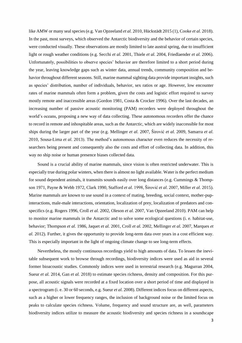
Passive acoustic data from January until November 2013 were collected about 480 km off the continent
Antarctica (Fig. 2a, 65° 58.09’ S, 12° 15.12’ W; Van Opzeeland et al. 2013 (1)). Continuous passive
acoustic recordings analyzed in this study, were conducted with the Sono.Vault recorder “AWI248-
01_SV1013” (Develogic GmbH, Hamburg, Germany) as part of the Hybrid Antarctic Float Observing
System (HAFOS, Fig. 2b) mooring network. HAFOS is a large-scale, long-term oceanographic obser-
vatory in the Weddell Sea, which contains 21 mooring positions equipped with a suite of oceanographic
devices as well as autonomous passive acoustic recorders. The utilized recorder was deployed in De-
cember 2012 during the expedition ANT-29/2 of research vessel “Polarstern” and recovered in January
2017 during the expedition PS103 with the same research ship. It was positioned in approximately 1081
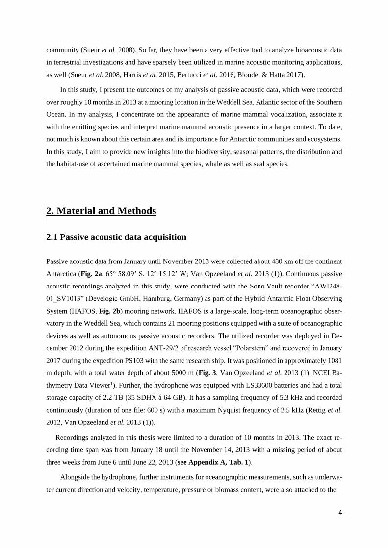
m depth, with a total water depth of about 5000 m (Fig. 3, Van Opzeeland et al. 2013 (1), NCEI Ba-
thymetry Data Viewer1). Further, the hydrophone was equipped with LS33600 batteries and had a total
storage capacity of 2.2 TB (35 SDHX á 64 GB). It has a sampling frequency of 5.3 kHz and recorded
continuously (duration of one file: 600 s) with a maximum Nyquist frequency of 2.5 kHz (Rettig et al.
2012, Van Opzeeland et al. 2013 (1)).
Recordings analyzed in this thesis were limited to a duration of 10 months in 2013. The exact re-
cording time span was from January 18 until the November 14, 2013 with a missing period of about
three weeks from June 6 until June 22, 2013 (see Appendix A, Tab. 1).
Alongside the hydrophone, further instruments for oceanographic measurements, such as underwa-
ter current direction and velocity, temperature, pressure or biomass content, were also attached to the
5
mooring station (Fig. 3, Boebel et al. 2013). Due to time restrictions, data collected by these devices
were not included in any of the analyses here.
2.2 Subsampling scheme
Since the hydrophone recorded continuously, the data needed to be subsampled so that a subset of the
data over the whole recording period was analyzed. A data subset was taken based on results from a
former unpublished analysis (Hots, unpublished). As part of the study, I ascertained the most fitting
subsampling scheme for the existing data (for approach see Appendix C). A sufficient scheme was
given by analyzing the first ten minutes of every hour. Hence, this subsampling scheme was applied to
the data that were analyzed in this thesis.
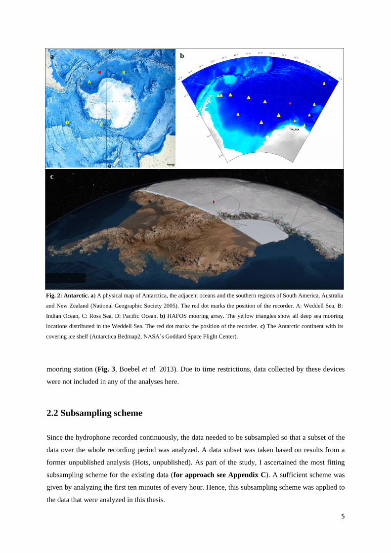
Fig. 2: Antarctic. a) A physical map of Antarctica, the adjacent oceans and the southern regions of South America, Australia
and New Zealand (National Geographic Society 2005). The red dot marks the position of the recorder. A: Weddell Sea, B:
Indian Ocean, C: Ross Sea, D: Pacific Ocean. b) HAFOS mooring array. The yellow triangles show all deep sea mooring
locations distributed in the Weddell Sea. The red dot marks the position of the recorder. c) The Antarctic continent with its
covering ice shelf (Antarctica Bedmap2, NASA’s Goddard Space Flight Center).
0
0a b
c
A
B
C D
6
2.3 Data analysis
2.3.1 Recordings
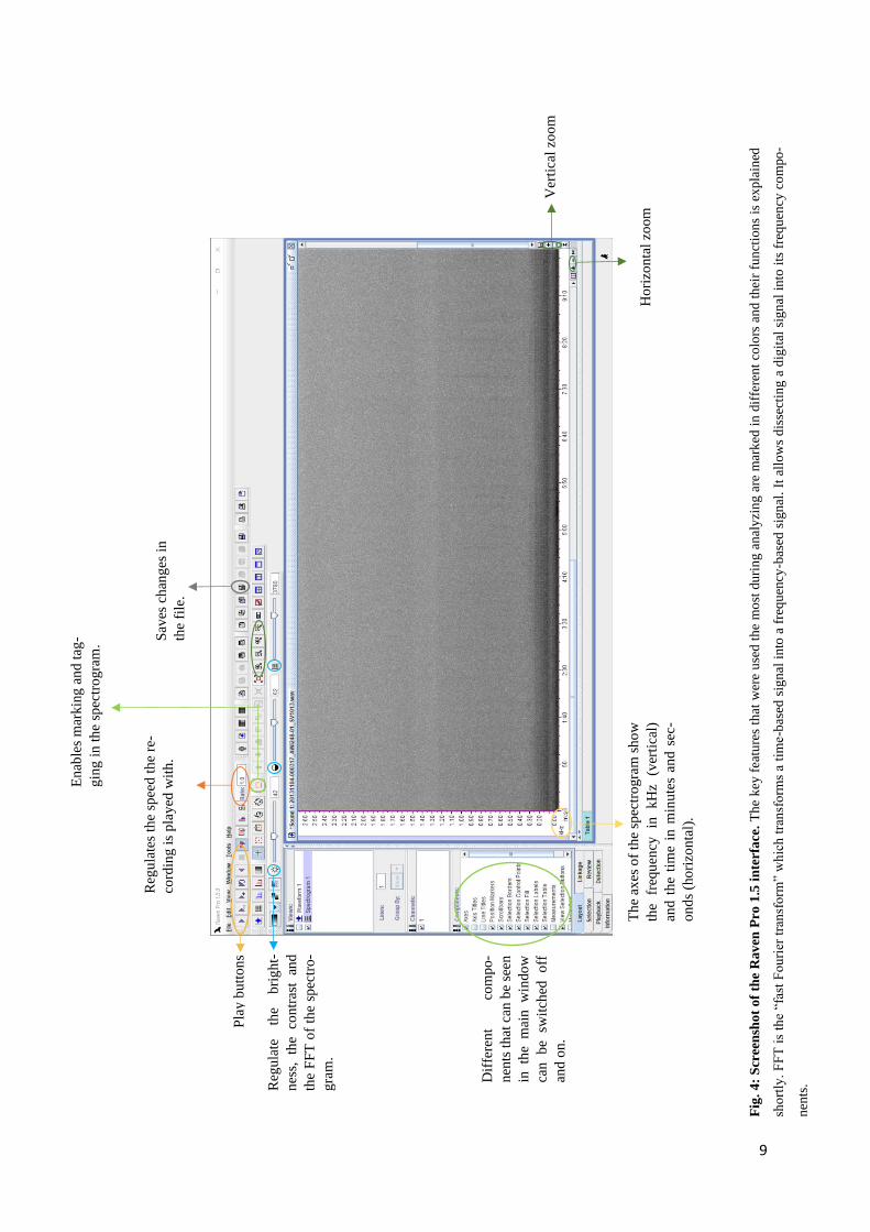
To analyze the data, I used Raven Pro 1.5 (Cornell Lab of Ornithology, Ithaca, NY, USA; Fig. 4). Since
the sound in the recordings had a low amplitude due to problems with the internal amplifier of the
recorder, each file was amplified (ampl.) by either 20 or 30 times. For every analysis, the spectrogram
parameters were set to a Hann or Hamming window, according to the sound analyzed and what window
presented a better resolution. Further, the Discrete Fourier Transform (DFT) was set to 512 samples for
every recording, the overlap, Fast Fourier Transform (FFT), brightness and contrast were adjusted inde-
pendently. FFT sizes ranged between 130 and 12714 points (pts), resulting in a time resolution (tr) with
its minimum at 0.05 s and maximum at 5 s: And a minimal and maximal frequency resolution (fr) of 0.2
Hz and 19.23 Hz. The spectrograms of the 10 min sound files were analyzed visually and aurally for the
presence of vocalization of marine mammals. Only the acoustic presence of marine mammal species-
specific acoustic signatures was logged on an hourly basis, so the number of acoustic signatures was not
counted. A species was considered present during a given hour if at least one call, known to be produced
by this species, was visually and aurally detected in the 10-min spectrogram. Detected vocalizations
were compared with already existing sound samples of the Alfred Wegener Institute, Bremerhaven,
Germany (in the following: AWI), spectrograms shown in other publications and sound-examples up-
loaded in online databases (e.g. NEFSC.NOAA.gov, Macaulaylibrary.org, Whalewatch.com3) associ-
ated to marine mammal vocalization to ensure a correct allocation between vocalization and species.
For the statistics, Excel 2010 (Microsoft Corporation, Redmond, WA, USA) and R 3.5.2 (R Core Team,
Vienna, AUT) were used.
To simplify the analysis, I refer in the following to “winter and summer months”. “Winter” here
refers to the months with forming or solid ice (October to March), whereas “summer” refers to the period
during which sea ice is (fast) retreating and ice-free months (April to September; see Appendix B).
2.3.2 Ice data
Results according the appearance of each species over the whole year, were further associated with data
of daily ice concentrations. Sea ice data were taken from satellite images of the Advanced Microwave
Scanning Radiometer for EOS (AMSR-E) satellite sensor (Spreen et al. 2008) with a resolution of 6.25
x 6.25 km per grid cell. Data were calculated for a radius of 30, 50 and 100 km off the mooring location.
Different radii were taken to include sea ice data for all observed species. Some species’ vocalization is
only transmit over some tens of kilometers (i.e. seals). However, calls of other species can travel over
3 See internet references.

7
Fig. 3: Mooring scheme of the station “AWI248-1” of the HAFOS mooring network. The scheme shows the instruments
mounted to the mooring station, as well as the depth in which they were vertically positioned. The Sono.Vault recorder was
positioned in water depth of about 1080 m. The ocean floor at that location is at 5051 m depth. It was mounted in 2012 and
recaptured in 2017. Further oceanographic instruments like SB 37 (SeaBird Electronics, Type: MicroCat, to measure Tem-
perature and Conductivity) or sound source (Develogic acoustic source for RAFOS floats, to track motion in the ocean
water) were also attached to mooring (Boebel et al. 2013; Figure by S. Spiesecke, AWI).
at
acoustic source
anchor
4 Floats
6 Floats
8
100 km (i.e. blue and fin whales). Hence, long ranged vocalization emitting animals can be distant from
the recorder by over 100 km, which is why ice data over a broad radius have to be taken into account,
when looking at acoustic data (e.g. Cumming & Thompson 1971, Payne & Webb 1971, Stafford et al.
1998, Širović et al. 2007).
2.3.3 Biodiversity Indices
In the last years, the usage of biodiversity indices for acoustic data has become more and more common
(e.g. Magurran 2004, Gan et al. 2018, Sueur et al. 2014). Indices are algorithms that can be applied to
bioacoustic recordings to obtain information on acoustic parameters of the sound environment, for ex-
ample calculating the species richness, evenness, regularity, divergence or rarity in species abundance
(Magurran 2004, Pavoine & Bonsall 2010, Magurran & McGill 2011, Sueur et al. 2014). Indices can be
categorized in within-group indices α (alpha) and between-group indices β (beta) (Whittaker 1972).
Results for each index tends towards 0 for only one pure tone in a recording and towards 1 for a high
sound diversity (Sueur et al. 2008). In this study, 13 α indices were used to automatically quantify the
overall species richness and compare it with my hand-browsed findings. The biodiversity indices were
applied on the marine bioacoustics data, using R 3.5.2.
3. Results
In this study, I was able to detect nine marine mammal species based on their species-specific vocaliza-
tions over the year of 2013. These included four baleen whale species (ABW, fin, humpback and AMW),
two toothed whale species (killer, Orcinus orca Fitzinger 1860, and sperm whales) and three seal species
(leopard, Hydrurga leptonyx Blainville 1820, crabeater, Lobodon carcinophaga Hombron & Jacquinot
1842, and Ross seals, Ommatophoca rossii Gray 1844). Some further detected sounds were likely linked
to biotic sources but could not be attributed to a specific source or species. Examples of the most com-
mon unidentified sounds are provided in section 3.4.1. The results are separated into three parts: First,
spectrograms of vocalizations that were attributed to species with certainty are provided. Detected
sounds are structured by sound emitting species (baleen whales, toothed whales, seals and unknown
sources). The second part of the results contains information on the temporal patterns in species’ acous-
tic presence and their relation to ice cover and the presence of other species. Finally, results for the
application of biodiversity indices on the analyzed recordings are provided in the third part.
9
Reg
ula
tes
the
spee
d t
he
re-
cord
ing i
s p
lay
ed w
ith
. S
aves
ch
ang
es i
n
the
file
.
Ver
tica
l zo
om
Ho
rizo
nta
l zo
om
T
he
axes
of
the
spec
tro
gra
m s
ho
w
the
freq
uen
cy
in
kH
z (v
erti
cal)
and
th
e ti
me
in m
inu
tes
and
sec
-
on
ds
(ho
rizo
nta
l).
Dif
fere
nt
com
po-
nen
ts t
hat
can
be
seen
in th
e m
ain
w
indo
w
can
b
e sw
itch
ed
off
and
on.
Reg
ula
te
the
bri
gh
t-
nes
s,
the
con
tras
t an
d
the
FF
T o
f th
e sp
ectr
o-
gra
m.
Pla
y b
utt
on
s
En
able
s m
ark
ing
an
d t
ag-
gin
g i
n t
he
spec
tro
gra
m.
Fig
. 4
: S
cree
nsh
ot
of
the
Rav
en P
ro 1
.5 i
nte
rfa
ce.
Th
e k
ey f
eatu
res
that
wer
e u
sed t
he
mo
st d
uri
ng
an
aly
zin
g a
re m
ark
ed i
n d
iffe
ren
t co
lors
an
d t
hei
r fu
nct
ion
s is
ex
pla
ined
sho
rtly
. F
FT
is
the
“fas
t F
ou
rier
tra
nsf
orm
” w
hic
h t
ran
sfo
rms
a ti
me-b
ased
sig
nal
in
to a
fre
qu
ency
-bas
ed s
ign
al.
It a
llo
ws
dis
sect
ing
a d
igit
al s
ign
al i
nto
its
fre
qu
ency
co
mpo
-
nen
ts.
10
3.1 Detected sounds
3.1.1 Baleen whales
Antarctic blue whales
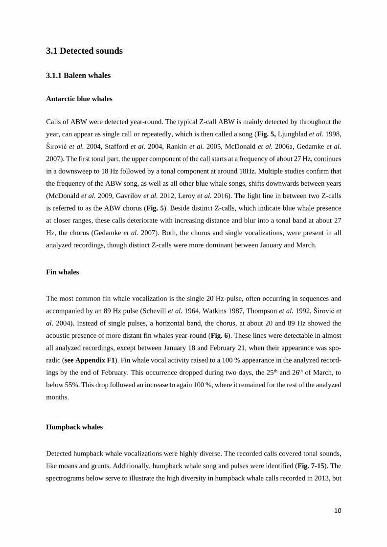
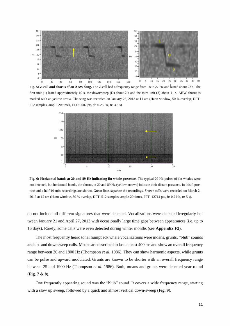
Calls of ABW were detected year-round. The typical Z-call ABW is mainly detected by throughout the
year, can appear as single call or repeatedly, which is then called a song (Fig. 5, Ljungblad et al. 1998,
Širović et al. 2004, Stafford et al. 2004, Rankin et al. 2005, McDonald et al. 2006a, Gedamke et al.
2007). The first tonal part, the upper component of the call starts at a frequency of about 27 Hz, continues
in a downsweep to 18 Hz followed by a tonal component at around 18Hz. Multiple studies confirm that
the frequency of the ABW song, as well as all other blue whale songs, shifts downwards between years
(McDonald et al. 2009, Gavrilov et al. 2012, Leroy et al. 2016). The light line in between two Z-calls
is referred to as the ABW chorus (Fig. 5). Beside distinct Z-calls, which indicate blue whale presence
at closer ranges, these calls deteriorate with increasing distance and blur into a tonal band at about 27
Hz, the chorus (Gedamke et al. 2007). Both, the chorus and single vocalizations, were present in all
analyzed recordings, though distinct Z-calls were more dominant between January and March.
Fin whales
The most common fin whale vocalization is the single 20 Hz-pulse, often occurring in sequences and
accompanied by an 89 Hz pulse (Schevill et al. 1964, Watkins 1987, Thompson et al. 1992, Širović et
al. 2004). Instead of single pulses, a horizontal band, the chorus, at about 20 and 89 Hz showed the
acoustic presence of more distant fin whales year-round (Fig. 6). These lines were detectable in almost
all analyzed recordings, except between January 18 and February 21, when their appearance was spo-
radic (see Appendix F1). Fin whale vocal activity raised to a 100 % appearance in the analyzed record-
ings by the end of February. This occurrence dropped during two days, the 25th and 26th of March, to
below 55%. This drop followed an increase to again 100 %, where it remained for the rest of the analyzed
months.
Humpback whales
Detected humpback whale vocalizations were highly diverse. The recorded calls covered tonal sounds,
like moans and grunts. Additionally, humpback whale song and pulses were identified (Fig. 7-15). The
spectrograms below serve to illustrate the high diversity in humpback whale calls recorded in 2013, but
11
do not include all different signatures that were detected. Vocalizations were detected irregularly be-
tween January 21 and April 27, 2013 with occasionally large time gaps between appearances (i.e. up to
16 days). Rarely, some calls were even detected during winter months (see Appendix F2).
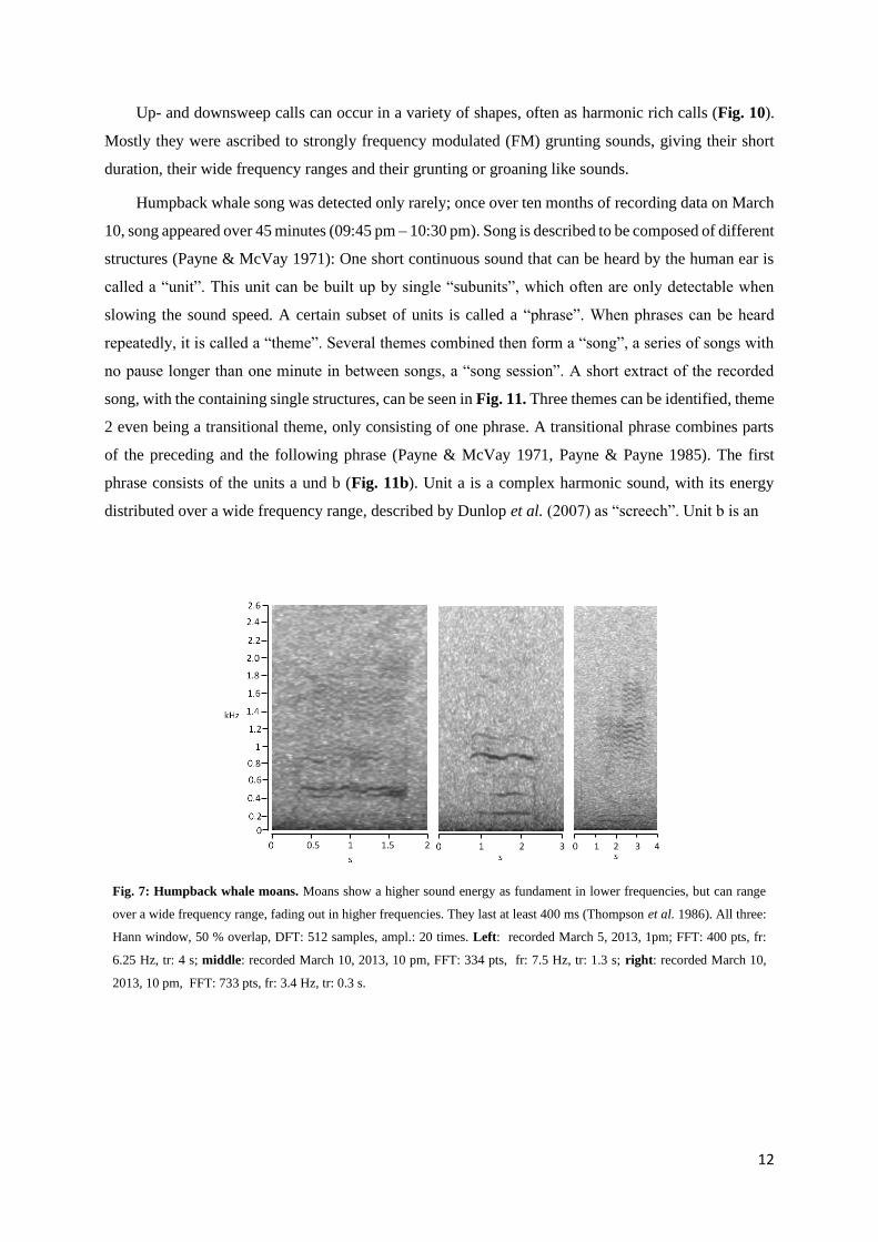
The most frequently heard tonal humpback whale vocalizations were moans, grunts, “blub” sounds
and up- and downsweep calls. Moans are described to last at least 400 ms and show an overall frequency
range between 20 and 1800 Hz (Thompson et al. 1986). They can show harmonic aspects, while grunts
can be pulse and upward modulated. Grunts are known to be shorter with an overall frequency range
between 25 and 1900 Hz (Thompson et al. 1986). Both, moans and grunts were detected year-round
(Fig. 7 & 8).
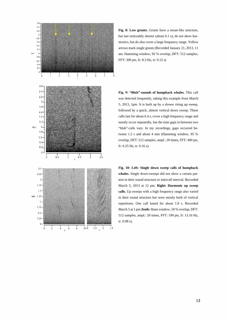
One frequently appearing sound was the “blub” sound. It covers a wide frequency range, starting
with a slow up sweep, followed by a quick and almost vertical down-sweep (Fig. 9).
Fig. 5: Z-call and chorus of an ABW song. The Z-call had a frequency range from 18 to 27 Hz and lasted about 23 s. The
first unit (1) lasted approximately 10 s, the downsweep (D) about 2 s and the third unit (3) about 11 s. ABW chorus is
marked with an yellow arrow. The song was recorded on January 28, 2013 at 11 am (Hann window, 50 % overlap, DFT:
512 samples, ampl.: 20 times, FFT: 9502 pts, fr: 0.26 Hz, tr: 3.8 s).
Fig. 6: Horizontal bands at 20 and 89 Hz indicating fin whale presence. The typical 20 Hz-pulses of fin whales were
not detected, but horizontal bands, the chorus, at 20 and 89 Hz (yellow arrows) indicate their distant presence. In this figure,
two and a half 10-min-recordings are shown. Green lines separate the recordings. Shown calls were recorded on March 2,
2013 at 12 am (Hann window, 50 % overlap, DFT: 512 samples, ampl.: 20 times, FFT: 12714 pts, fr: 0.2 Hz, tr: 5 s).
12
Up- and downsweep calls can occur in a variety of shapes, often as harmonic rich calls (Fig. 10).
Mostly they were ascribed to strongly frequency modulated (FM) grunting sounds, giving their short
duration, their wide frequency ranges and their grunting or groaning like sounds.
Humpback whale song was detected only rarely; once over ten months of recording data on March
10, song appeared over 45 minutes (09:45 pm – 10:30 pm). Song is described to be composed of different
structures (Payne & McVay 1971): One short continuous sound that can be heard by the human ear is
called a “unit”. This unit can be built up by single “subunits”, which often are only detectable when
slowing the sound speed. A certain subset of units is called a “phrase”. When phrases can be heard
repeatedly, it is called a “theme”. Several themes combined then form a “song”, a series of songs with
no pause longer than one minute in between songs, a “song session”. A short extract of the recorded
song, with the containing single structures, can be seen in Fig. 11. Three themes can be identified, theme
2 even being a transitional theme, only consisting of one phrase. A transitional phrase combines parts
of the preceding and the following phrase (Payne & McVay 1971, Payne & Payne 1985). The first
phrase consists of the units a und b (Fig. 11b). Unit a is a complex harmonic sound, with its energy
distributed over a wide frequency range, described by Dunlop et al. (2007) as “screech”. Unit b is an
Fig. 7: Humpback whale moans. Moans show a higher sound energy as fundament in lower frequencies, but can range
over a wide frequency range, fading out in higher frequencies. They last at least 400 ms (Thompson et al. 1986). All three:
Hann window, 50 % overlap, DFT: 512 samples, ampl.: 20 times. Left: recorded March 5, 2013, 1pm; FFT: 400 pts, fr:
6.25 Hz, tr: 4 s; middle: recorded March 10, 2013, 10 pm, FFT: 334 pts, fr: 7.5 Hz, tr: 1.3 s; right: recorded March 10,
2013, 10 pm, FFT: 733 pts, fr: 3.4 Hz, tr: 0.3 s.
13
Fig. 8: Low grunts. Grunts have a moan-like structure,
but last noticeably shorter (about 0.1 s), do not show har-
monics, but do also cover a large frequency range. Yellow
arrows mark single grunts (Recorded January 21, 2013, 11
am. Hamming window, 92 % overlap, DFT: 512 samples,
FFT: 300 pts, fr: 8.3 Hz, tr: 0.12 s)
Fig. 9: “Blub”-sounds of humpback whales. This call
was detected frequently, taking this example from March
5, 2013, 1pm. It is built up by a slower rising up sweep,
followed by a quick, almost vertical down sweep. These
calls last for about 0.4 s, cover a high frequency range and
mostly occur repeatedly, but the time gaps in between two
“blub”-calls vary. In my recordings, gaps occurred be-
tween 1.2 s and about 4 min (Hamming window, 95 %
overlap, DFT: 512 samples, ampl.: 20 times, FFT: 400 pts,
fr: 6.25 Hz, tr: 0.16 s).
Fig. 10: Left: Single down sweep calls of humpback
whales. Single down-sweeps did not show a certain pat-
tern in their sound structure or intercall interval. Recorded
March 5, 2013 at 12 pm. Right: Harmonic up sweep
calls. Up sweeps with a high frequency range also varied
in their sound structure but were mostly built of vertical
repetitions. One call lasted for about 1.8 s. Recorded
March 5 at 1 pm (both: Hann window, 50 % overlap, DFT:
512 samples, ampl.: 20 times, FFT: 190 pts, fr: 13.16 Hz,
tr: 0.08 s).

14
Fig. 11: Humpback whale song. a) The shown humpback whale song was recorded March 10, 2013 and lasted for approxi-
mately 45 minutes. Here only an extract of about two minutes is shown. Single components (unit, phrase, theme) can be identi-
fied and are marked in the figure. Phrases are composed by the units a, b and c (shown above the spectrogram), displayed as
close-ups in b) - d). Theme 2 only consists of one phrase; because it contains parts of the former and the following phrase, it is
called a transitional phrase (Payne & McVay 1971, Payne & Payne 1985). a) Hann window, 50 % overlap, DFT: 512 samples,
FFT: 360 pts, fr: 6.8 Hz , tr: 0.15 s. b)-d) Hamming window, 90 % overlap, DFT: 512 samples, ampl.: 20 times. b) FFT: 420
pts, fr: 6 Hz, tr: 0.16 s. c) FFT: 360 pts, fr: 7 Hz, tr: 0.14 s. d) FFT: 350 pts, fr: 7 Hz, tr: 0.14 s.
b) c)
d)
a)
15
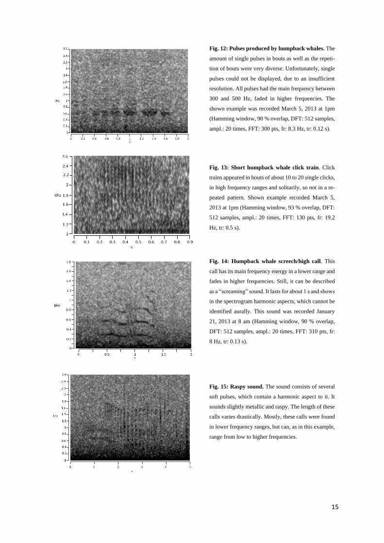
Fig. 12: Pulses produced by humpback whales. The
amount of single pulses in bouts as well as the repeti-
tion of bouts were very diverse. Unfortunately, single
pulses could not be displayed, due to an insufficient
resolution. All pulses had the main frequency between
300 and 500 Hz, faded in higher frequencies. The
shown example was recorded March 5, 2013 at 1pm
(Hamming window, 90 % overlap, DFT: 512 samples,
ampl.: 20 times, FFT: 300 pts, fr: 8.3 Hz, tr: 0.12 s).
Fig. 13: Short humpback whale click train. Click
trains appeared in bouts of about 10 to 20 single clicks,
in high frequency ranges and solitarily, so not in a re-
peated pattern. Shown example recorded March 5,
2013 at 1pm (Hamming window, 93 % overlap, DFT:
512 samples, ampl.: 20 times, FFT: 130 pts, fr: 19.2
Hz, tr: 0.5 s).
Fig. 14: Humpback whale screech/high call. This
call has its main frequency energy in a lower range and
fades in higher frequencies. Still, it can be described
as a “screaming” sound. It lasts for about 1 s and shows
in the spectrogram harmonic aspects, which cannot be
identified aurally. This sound was recorded January
21, 2013 at 8 am (Hamming window, 90 % overlap,
DFT: 512 samples, ampl.: 20 times, FFT: 310 pts, fr:
8 Hz, tr: 0.13 s).
Fig. 15: Raspy sound. The sound consists of several
soft pulses, which contain a harmonic aspect to it. It
sounds slightly metallic and raspy. The length of these
calls varies drastically. Mostly, these calls were found
in lower frequency ranges, but can, as in this example,
range from low to higher frequencies.
16
amplitude-modulated vocalization, but still shows harmonic components. Dunlop et al. (2007) described
this sound as “growl”. Its frequency, as well as in unit a, is broadly distributed. Both sounds are associ-
ated with song (Dunlop et al. 2007). The last unit of the shown extract, c, is a harmonic upsweep sound
with a wide frequency range, too. Sometimes a very short hook-like angle can be seen at the end of the
sound, continuing horizontally or downwards. Its sound reminds of a soft cry or siren.
As already mentioned, humpback whale vocalization is very diverse and colorful. Beside the pre-
sented calls and song, the most detected sounds contained pulses, clicks and screaming sounds
(“screech”: Dunlop et al. 2007, “high call”: Van Opzeeland et al. 2013 (2)), as well as raspy grunting
low frequency sounds (Fig. 12-15). The raspy sound does not match with the sound description of a
“wop” sound as described in Dunlop et al. (2007). Still, Stimpert et al. (2011) took this sound description
up again and showed a sound structure, which is very similar to what can be seen in Fig. 15. The raspy
sound could therefore be the described “wop” sound (Dunlop et al. 2007), but was not possible to clar-
ified fully.
Antarctic minke whales
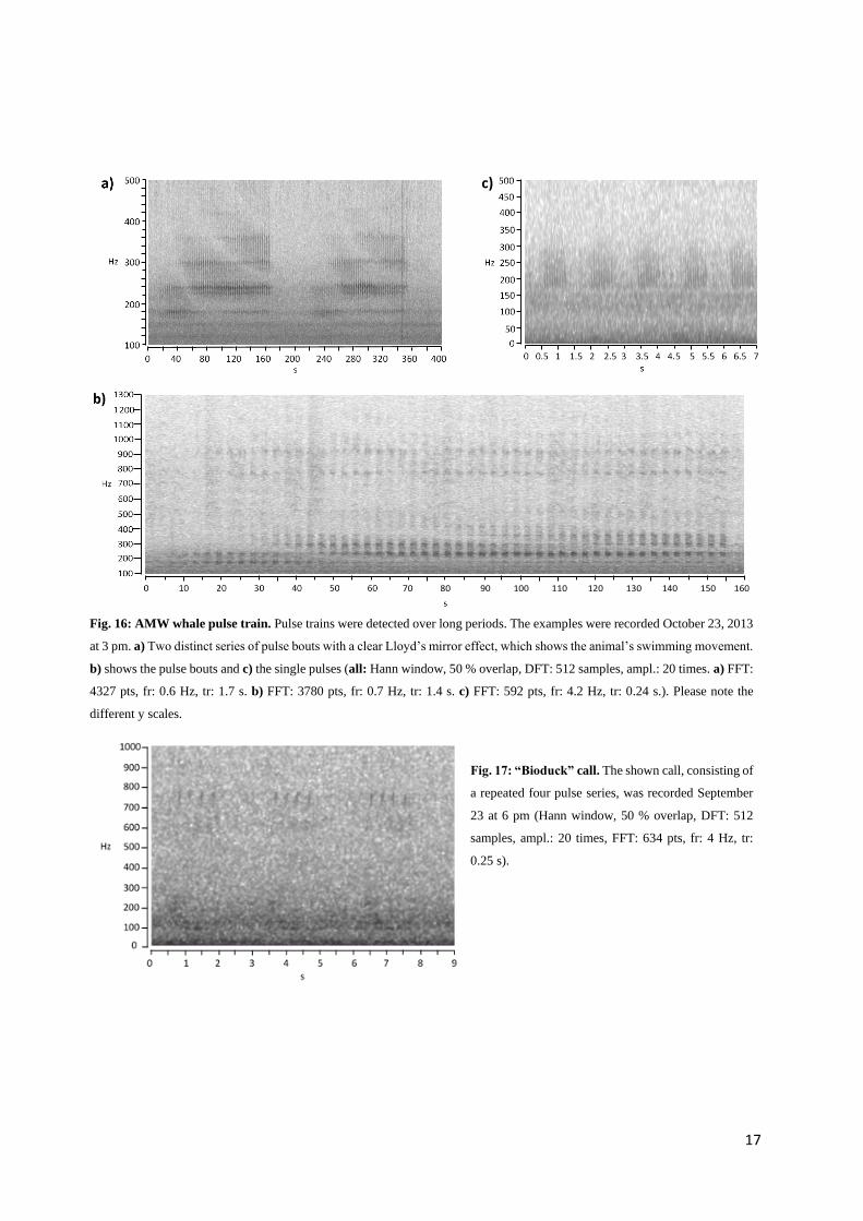
AMW were detected from the May 16 until November 14, 2013. In May and June, the appearances were
more sporadic, from July until the mid-November almost continuously (see Appendix F3). AMW were
recognized by their typical vocalization of continuous pulse trains (Mellinger et al. 2000, Risch et al.
2013). The pulses showed a duration of about 0.1 s and interpulse intervals of about the same length.
Longer pauses occurred after about 40 to 50 of these short pulses for mainly about 1 s, before the next
series of pulses started, but pausing time also varied from time to time (Fig. 16). For AMW it was not
unusual to detect these continuous vocalizations over a long period, i.e. such as 37, 46 or even 82 hours.
The prominent “bio-duck” call (Risch et al. 2014), which consisted of a repeated series of four
pulses mainly around 750 Hz, was also detected (Fig. 17), but rather rarely.
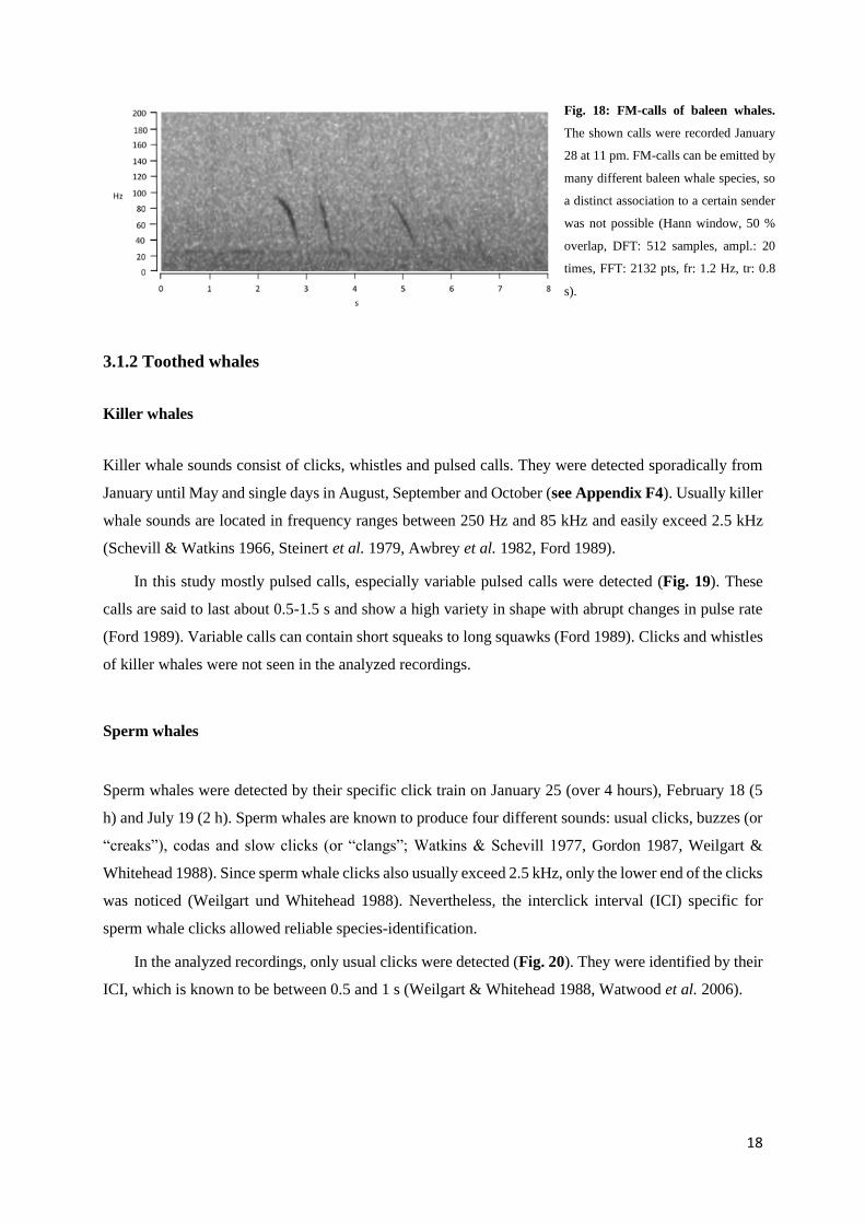
FM-calls
Many baleen whales produce the so-called “FM-calls” (Fig. 18). The calls are documented for ABW
(Rankin et al. 2005), fin whales (Watkins 1981) and AMW (Dominello & Sivoric 2016). FM-calls are
frequency modulated down sweeps and occur between 25 and 100 Hz (Oleson et al. 2007, Lewis et al.
2018). Since FM-calls show the same structure independent of the originator, it was impossible to sort
the calls to certain species.
17
Fig. 16: AMW whale pulse train. Pulse trains were detected over long periods. The examples were recorded October 23, 2013
at 3 pm. a) Two distinct series of pulse bouts with a clear Lloyd’s mirror effect, which shows the animal’s swimming movement.
b) shows the pulse bouts and c) the single pulses (all: Hann window, 50 % overlap, DFT: 512 samples, ampl.: 20 times. a) FFT:
4327 pts, fr: 0.6 Hz, tr: 1.7 s. b) FFT: 3780 pts, fr: 0.7 Hz, tr: 1.4 s. c) FFT: 592 pts, fr: 4.2 Hz, tr: 0.24 s.). Please note the
different y scales.
Fig. 17: “Bioduck” call. The shown call, consisting of
a repeated four pulse series, was recorded September
23 at 6 pm (Hann window, 50 % overlap, DFT: 512
samples, ampl.: 20 times, FFT: 634 pts, fr: 4 Hz, tr:
0.25 s).
c)
18
3.1.2 Toothed whales
Killer whales
Killer whale sounds consist of clicks, whistles and pulsed calls. They were detected sporadically from
January until May and single days in August, September and October (see Appendix F4). Usually killer
whale sounds are located in frequency ranges between 250 Hz and 85 kHz and easily exceed 2.5 kHz
(Schevill & Watkins 1966, Steinert et al. 1979, Awbrey et al. 1982, Ford 1989).
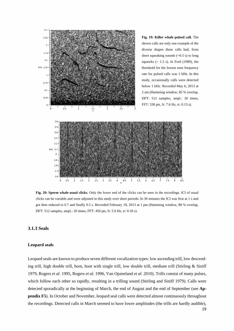
In this study mostly pulsed calls, especially variable pulsed calls were detected (Fig. 19). These
calls are said to last about 0.5-1.5 s and show a high variety in shape with abrupt changes in pulse rate
(Ford 1989). Variable calls can contain short squeaks to long squawks (Ford 1989). Clicks and whistles
of killer whales were not seen in the analyzed recordings.
Sperm whales
Sperm whales were detected by their specific click train on January 25 (over 4 hours), February 18 (5
h) and July 19 (2 h). Sperm whales are known to produce four different sounds: usual clicks, buzzes (or
“creaks”), codas and slow clicks (or “clangs”; Watkins & Schevill 1977, Gordon 1987, Weilgart &
Whitehead 1988). Since sperm whale clicks also usually exceed 2.5 kHz, only the lower end of the clicks
was noticed (Weilgart und Whitehead 1988). Nevertheless, the interclick interval (ICI) specific for
sperm whale clicks allowed reliable species-identification.
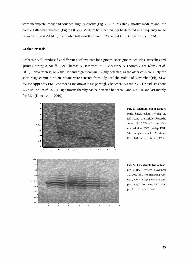
In the analyzed recordings, only usual clicks were detected (Fig. 20). They were identified by their
ICI, which is known to be between 0.5 and 1 s (Weilgart & Whitehead 1988, Watwood et al. 2006).
Fig. 18: FM-calls of baleen whales.
The shown calls were recorded January
28 at 11 pm. FM-calls can be emitted by
many different baleen whale species, so
a distinct association to a certain sender
was not possible (Hann window, 50 %
overlap, DFT: 512 samples, ampl.: 20
times, FFT: 2132 pts, fr: 1.2 Hz, tr: 0.8
s).
19
Fig. 19: Killer whale pulsed call. The
shown calls are only one example of the
diverse shapes these calls had, from
short squeaking sounds (~0.5 s) to long
squawks (~ 1.5 s). In Ford (1989), the
threshold for the lowest seen frequency
rate for pulsed calls was 1 kHz. In this
study, occasionally calls were detected
below 1 kHz. Recorded May 6, 2013 at
2 am (Hamming window, 85 % overlap,
DFT: 512 samples, ampl.: 20 times,
FFT: 330 pts, fr: 7.6 Hz, tr: 0.13 s).
Fig. 20: Sperm whale usual clicks. Only the lower end of the clicks can be seen in the recordings. ICI of usual
clicks can be variable and were adjusted in this study over short periods: In 30 minutes the ICI was first at 1 s and
got then reduced to 0.7 and finally 0.5 s. Recorded February 18, 2013 at 1 pm (Hamming window, 88 % overlap,
DFT: 512 samples, ampl.: 20 times, FFT: 450 pts, fr: 5.6 Hz, tr: 0.18 s).
3.1.3 Seals
Leopard seals
Leopard seals are known to produce seven different vocalization types: low ascending trill, low descend-
ing trill, high double trill, hoot, hoot with single trill, low double trill, medium trill (Stirling & Siniff
1979, Rogers et al. 1995, Rogers et al. 1996, Van Opzeeland et al. 2010). Trills consist of many pulses,
which follow each other so rapidly, resulting in a trilling sound (Stirling and Siniff 1979). Calls were
detected sporadically at the beginning of March, the end of August and the end of September (see Ap-
pendix F5). In October and November, leopard seal calls were detected almost continuously throughout
the recordings. Detected calls in March seemed to have lower amplitudes (the trills are hardly audible),
20
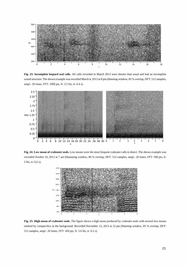
were incomplete, awry and sounded slightly croaky (Fig. 23). In this study, mostly medium and low
double trills were detected (Fig. 21 & 22). Medium trills can mainly be detected in a frequency range
between 1.3 and 2.4 kHz, low double trills mostly between 230 and 430 Hz (Rogers et al. 1995).
Crabeater seals
Crabeater seals produce five different vocalizations: long groans, short groans, whistles, screeches and
grunts (Stirling & Siniff 1979, Thomas & DeMaster 1982, McCreery & Thomas 2009, Klinck et al.
2010). Nevertheless, only the low and high moan are usually detected, as the other calls are likely for
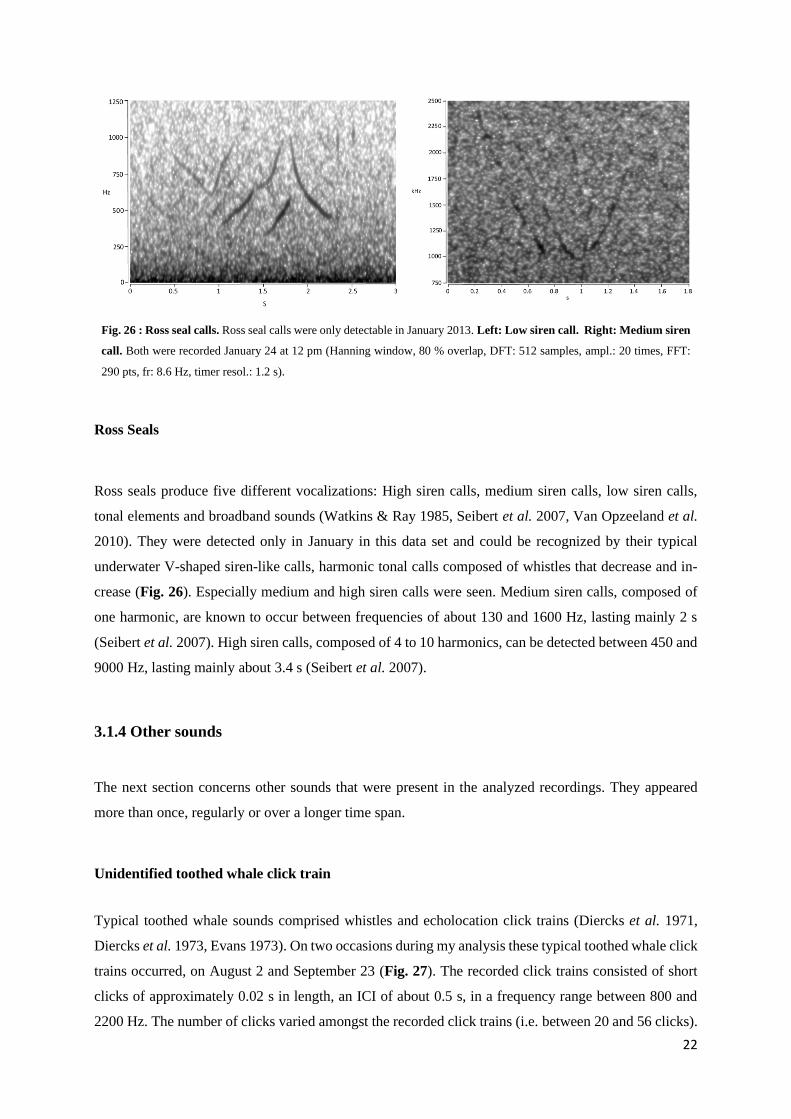
short-range communication. Moans were detected from July until the middle of November (Fig. 24 &
25, see Appendix F6). Low moans are known to range roughly between 260 and 2500 Hz and last about
2.5 s (Klinck et al. 2010). High moans thereby can be detected between 1 and 4.9 kHz and last mainly
for 2.6 s (Klinck et al. 2010).
Fig. 21: Medium trill of leopard
seals. Single pulses, forming the
trill sound, are visible. Recorded
August 24, 2013 at 11 pm (Han-
ning window, 85% overlap, DFT:
512 samples, ampl.: 20 times,
FFT: 420 pts, fr: 6 Hz, tr: 0.17 s).
Fig. 22: Low double trill of leop-
ard seals. Recorded November
12, 2013 at 0 pm (Hanning win-
dow, 80% overlap, DFT: 512 sam-
ples, ampl.: 20 times, FFT: 1500
pts, fr: 1.7 Hz, tr: 0.06 s).
21
Fig. 23: Incomplete leopard seal calls. All calls recorded in March 2013 were shorter than usual and had an incomplete
sound structure. The shown example was recorded March 4, 2013 at 8 pm (Hanning window, 85 % overlap, DFT: 512 samples,
ampl.: 20 times, FFT: 1000 pts, fr: 2.5 Hz, tr: 0.4 s).
Fig. 24: Low moan of crabeater seals. Low moans were the most frequent crabeater calls to detect. The shown example was
recorded October 10, 2013 at 7 am (Hamming window, 80 % overlap, DFT: 512 samples, ampl.: 20 times, FFT: 580 pts, fr:
5 Hz, tr: 0,2 s).
Fig. 25: High moan of crabeater seals. The figure shows a high moan produced by crabeater seals with several low moans
emitted by conspecifics in the background. Recorded November 12, 2013 at 12 pm (Hanning window, 85 % overlap, DFT:
512 samples, ampl.: 20 times, FFT: 450 pts, fr: 5.6 Hz, tr: 0.2 s).
22
Ross Seals
Ross seals produce five different vocalizations: High siren calls, medium siren calls, low siren calls,
tonal elements and broadband sounds (Watkins & Ray 1985, Seibert et al. 2007, Van Opzeeland et al.
2010). They were detected only in January in this data set and could be recognized by their typical
underwater V-shaped siren-like calls, harmonic tonal calls composed of whistles that decrease and in-
crease (Fig. 26). Especially medium and high siren calls were seen. Medium siren calls, composed of
one harmonic, are known to occur between frequencies of about 130 and 1600 Hz, lasting mainly 2 s
(Seibert et al. 2007). High siren calls, composed of 4 to 10 harmonics, can be detected between 450 and
9000 Hz, lasting mainly about 3.4 s (Seibert et al. 2007).
3.1.4 Other sounds
The next section concerns other sounds that were present in the analyzed recordings. They appeared
more than once, regularly or over a longer time span.
Unidentified toothed whale click train
Typical toothed whale sounds comprised whistles and echolocation click trains (Diercks et al. 1971,
Diercks et al. 1973, Evans 1973). On two occasions during my analysis these typical toothed whale click
trains occurred, on August 2 and September 23 (Fig. 27). The recorded click trains consisted of short
clicks of approximately 0.02 s in length, an ICI of about 0.5 s, in a frequency range between 800 and
2200 Hz. The number of clicks varied amongst the recorded click trains (i.e. between 20 and 56 clicks).
Fig. 26 : Ross seal calls. Ross seal calls were only detectable in January 2013. Left: Low siren call. Right: Medium siren
call. Both were recorded January 24 at 12 pm (Hanning window, 80 % overlap, DFT: 512 samples, ampl.: 20 times, FFT:
290 pts, fr: 8.6 Hz, timer resol.: 1.2 s).
23
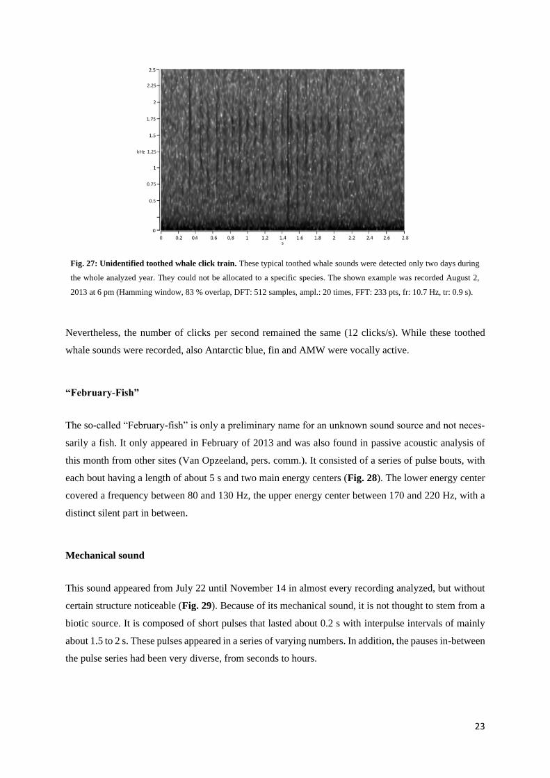
Nevertheless, the number of clicks per second remained the same (12 clicks/s). While these toothed
whale sounds were recorded, also Antarctic blue, fin and AMW were vocally active.
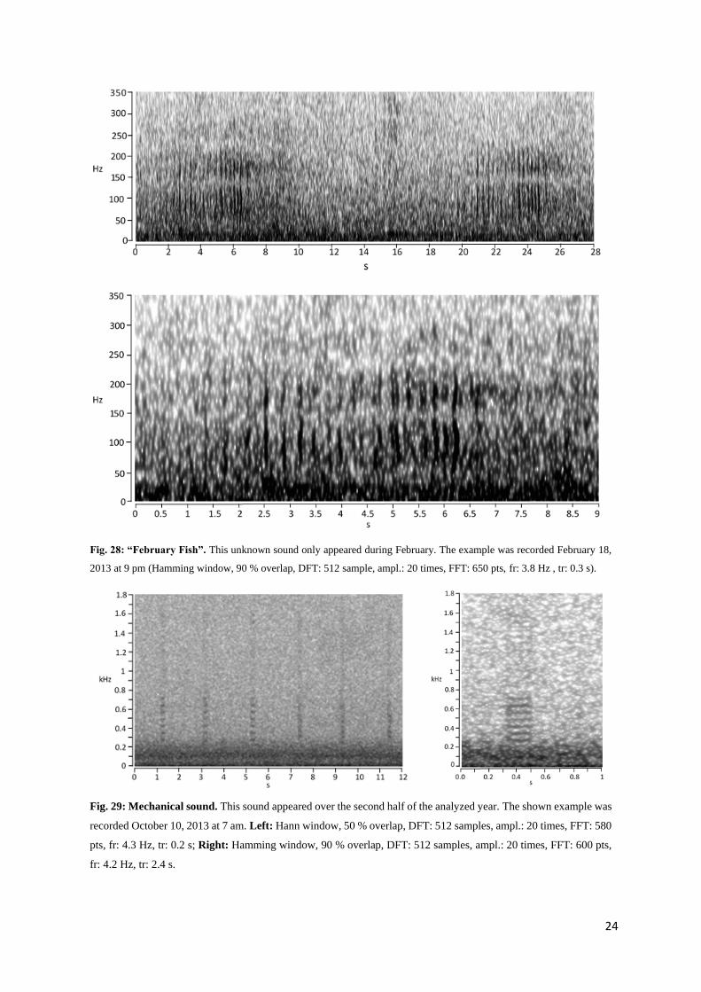
“February-Fish”
The so-called “February-fish” is only a preliminary name for an unknown sound source and not neces-
sarily a fish. It only appeared in February of 2013 and was also found in passive acoustic analysis of
this month from other sites (Van Opzeeland, pers. comm.). It consisted of a series of pulse bouts, with
each bout having a length of about 5 s and two main energy centers (Fig. 28). The lower energy center
covered a frequency between 80 and 130 Hz, the upper energy center between 170 and 220 Hz, with a
distinct silent part in between.
Mechanical sound
This sound appeared from July 22 until November 14 in almost every recording analyzed, but without
certain structure noticeable (Fig. 29). Because of its mechanical sound, it is not thought to stem from a
biotic source. It is composed of short pulses that lasted about 0.2 s with interpulse intervals of mainly
about 1.5 to 2 s. These pulses appeared in a series of varying numbers. In addition, the pauses in-between
the pulse series had been very diverse, from seconds to hours.
Fig. 27: Unidentified toothed whale click train. These typical toothed whale sounds were detected only two days during
the whole analyzed year. They could not be allocated to a specific species. The shown example was recorded August 2,
2013 at 6 pm (Hamming window, 83 % overlap, DFT: 512 samples, ampl.: 20 times, FFT: 233 pts, fr: 10.7 Hz, tr: 0.9 s).
24
Fig. 28: “February Fish”. This unknown sound only appeared during February. The example was recorded February 18,
2013 at 9 pm (Hamming window, 90 % overlap, DFT: 512 sample, ampl.: 20 times, FFT: 650 pts, fr: 3.8 Hz , tr: 0.3 s).
Fig. 29: Mechanical sound. This sound appeared over the second half of the analyzed year. The shown example was
recorded October 10, 2013 at 7 am. Left: Hann window, 50 % overlap, DFT: 512 samples, ampl.: 20 times, FFT: 580
pts, fr: 4.3 Hz, tr: 0.2 s; Right: Hamming window, 90 % overlap, DFT: 512 samples, ampl.: 20 times, FFT: 600 pts,
fr: 4.2 Hz, tr: 2.4 s.
25
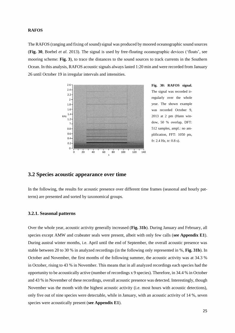
RAFOS
The RAFOS (ranging and fixing of sound) signal was produced by moored oceanographic sound sources
(Fig. 30, Boebel et al. 2013). The signal is used by free-floating oceanographic devices (‘floats’, see
mooring scheme: Fig. 3), to trace the distances to the sound sources to track currents in the Southern
Ocean. In this analysis, RAFOS acoustic signals always lasted 1:20 min and were recorded from January
26 until October 19 in irregular intervals and intensities.
3.2 Species acoustic appearance over time
In the following, the results for acoustic presence over different time frames (seasonal and hourly pat-
terns) are presented and sorted by taxonomical groups.
3.2.1. Seasonal patterns
Over the whole year, acoustic activity generally increased (Fig. 31b). During January and February, all
species except AMW and crabeater seals were present, albeit with only few calls (see Appendix E1).
During austral winter months, i.e. April until the end of September, the overall acoustic presence was
stable between 20 to 30 % in analyzed recordings (in the following only represented in %, Fig. 31b). In
October and November, the first months of the following summer, the acoustic activity was at 34.3 %
in October, rising to 43 % in November. This means that in all analyzed recordings each species had the
opportunity to be acoustically active (number of recordings x 9 species). Therefore, in 34.4 % in October
and 43 % in November of these recordings, overall acoustic presence was detected. Interestingly, though
November was the month with the highest acoustic activity (i.e. most hours with acoustic detections),
only five out of nine species were detectable, while in January, with an acoustic activity of 14 %, seven
species were acoustically present (see Appendix E1).
Fig. 30: RAFOS signal.
The signal was recorded ir-
regularly over the whole
year. The shown example
was recorded October 9,
2013 at 2 pm (Hann win-
dow, 50 % overlap, DFT:
512 samples, ampl.: no am-
plification, FFT: 1050 pts,
fr: 2.4 Hz, tr: 0.8 s).
26
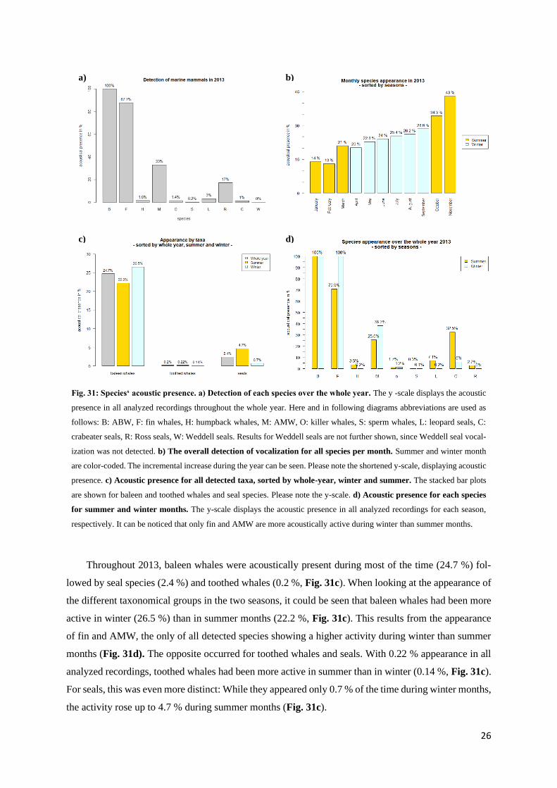
Throughout 2013, baleen whales were acoustically present during most of the time (24.7 %) fol-
lowed by seal species (2.4 %) and toothed whales (0.2 %, Fig. 31c). When looking at the appearance of
the different taxonomical groups in the two seasons, it could be seen that baleen whales had been more
active in winter (26.5 %) than in summer months (22.2 %, Fig. 31c). This results from the appearance
of fin and AMW, the only of all detected species showing a higher activity during winter than summer
months (Fig. 31d). The opposite occurred for toothed whales and seals. With 0.22 % appearance in all
analyzed recordings, toothed whales had been more active in summer than in winter (0.14 %, Fig. 31c).
For seals, this was even more distinct: While they appeared only 0.7 % of the time during winter months,
the activity rose up to 4.7 % during summer months (Fig. 31c).
Fig. 31: Species‘ acoustic presence. a) Detection of each species over the whole year. The y -scale displays the acoustic
presence in all analyzed recordings throughout the whole year. Here and in following diagrams abbreviations are used as
follows: B: ABW, F: fin whales, H: humpback whales, M: AMW, O: killer whales, S: sperm whales, L: leopard seals, C:
crabeater seals, R: Ross seals, W: Weddell seals. Results for Weddell seals are not further shown, since Weddell seal vocal-
ization was not detected. b) The overall detection of vocalization for all species per month. Summer and winter month
are color-coded. The incremental increase during the year can be seen. Please note the shortened y-scale, displaying acoustic
presence. c) Acoustic presence for all detected taxa, sorted by whole-year, winter and summer. The stacked bar plots
are shown for baleen and toothed whales and seal species. Please note the y-scale. d) Acoustic presence for each species
for summer and winter months. The y-scale displays the acoustic presence in all analyzed recordings for each season,
respectively. It can be noticed that only fin and AMW are more acoustically active during winter than summer months.
a) b)
c) d)

27
3.2.1.1 Baleen whales
Antarctic blue whales
ABW were detectable in every recording analyzed (100 % appearance in all analyzed recordings, Fig.
31a). Detections included nearby single calls and song (Z-call), as well as chorus of distant animals.
Fin whales
Following ABW, fin whales appeared the second most of all species (87.7 %, Fig. 31a). As well as for
ABW, nearby single pulses, as well as chorus are included in this value. Fin whales appeared throughout
the recordings in winter, while only being present for about 70 % during summer months (Fig. 31d):
Between the first analyzed recording (January 18) and February 21, fin whales were detectable, but only
very sporadically. The same can be noticed between the 25th and 26th of March. Nevertheless, after
March 26 the activity rose to 100 % and remained at this level throughout the rest of the analyzed
recordings (see Appendix F1).
Humpback whales
In comparison to that, the fourth baleen whale species, humpback whales, only appeared for 1.6 % over
the whole year (Fig. 31a). This means that calls were detected in only about 100 analyzed recordings
(i.e. 10-minute files), spread over 25 noncontiguous days (see Appendix F2 & Appendix G). These
days were shared by 21 days during the summer months (October – March, see Appendix G), where
humpback whale calls cover 3.5 % of the whole detections in this season, and four days during winter
months (April – September) with 0.2 % appearance of all analyzed recordings in that season (Fig. 31d,
see Appendix G).
The strongest acoustic activity could be seen in the first months of the year. March stood out by far
with even 10 % appearance (see Appendix F). This means, in contrast to the results of the other three
baleen whales (esp. fin and AMW), humpback whales were much more acoustically active during sum-
mer than winter (Fig. 31d).
Antarctic minke whales
AMW appeared 33 % in all analyzed recordings (Fig. 31a). During summer, they were detected 25.6 %
and even more during winter (38.3 %, Fig. 31d). While there had been sporadic calls in the months of
May and June, the activity rose noticeably from July (52 %) to November (78 %, see Appendix E1).
28
3.2.1.2 Toothed whales
Killer whales
Toothed whales appeared acoustically rare over the whole year. Killer whales showed an overall ap-
pearance of 1.4 % for the whole year (Fig. 31a), in 1.7 % of all analyzed recordings during summer (18
d) and 1.2 % during winter (13 d, Fig. 31d, see Appendix G). The highest activity was detected in
March and May, the lowest in August, September and October (see Appendix E2). In June, July and
November killer whales were not detected at all.
Sperm whales
Sperm whales were detected only on three days, which means 0.2 % throughout the whole year (Fig.
31a, see Appendix G). During the summer months, sperm whales appeared on January 25 and February
18, in winter on the 19th of July. On these days, their clicks had been recorded for two to five hours (see
Appendix G).
3.2.1.3 Seals
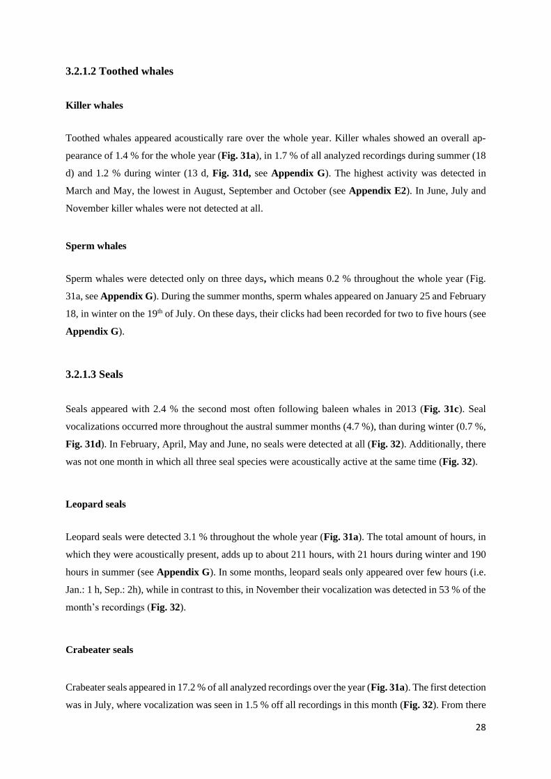
Seals appeared with 2.4 % the second most often following baleen whales in 2013 (Fig. 31c). Seal
vocalizations occurred more throughout the austral summer months (4.7 %), than during winter (0.7 %,
Fig. 31d). In February, April, May and June, no seals were detected at all (Fig. 32). Additionally, there
was not one month in which all three seal species were acoustically active at the same time (Fig. 32).
Leopard seals
Leopard seals were detected 3.1 % throughout the whole year (Fig. 31a). The total amount of hours, in
which they were acoustically present, adds up to about 211 hours, with 21 hours during winter and 190
hours in summer (see Appendix G). In some months, leopard seals only appeared over few hours (i.e.
Jan.: 1 h, Sep.: 2h), while in contrast to this, in November their vocalization was detected in 53 % of the
month’s recordings (Fig. 32).
Crabeater seals
Crabeater seals appeared in 17.2 % of all analyzed recordings over the year (Fig. 31a). The first detection
was in July, where vocalization was seen in 1.5 % off all recordings in this month (Fig. 32). From there
29
abundance grew steadily to a 100 % appearance in November (Fig. 32). Of all seal species, crabeater
seals appeared the most in both seasons, followed by leopard seals (Fig. 31d). Between August and
November both seal species occurred together (Fig. 32).
Ross seals
Ross seals were only detected in January (Fig. 32). Its acoustic presence was detected in 24% of all
recordings in January and in 1.1 % of all recordings throughout the whole year (Fig. 31a).
3.2.2 Hourly patterns
3.2.2.1 Baleen whales
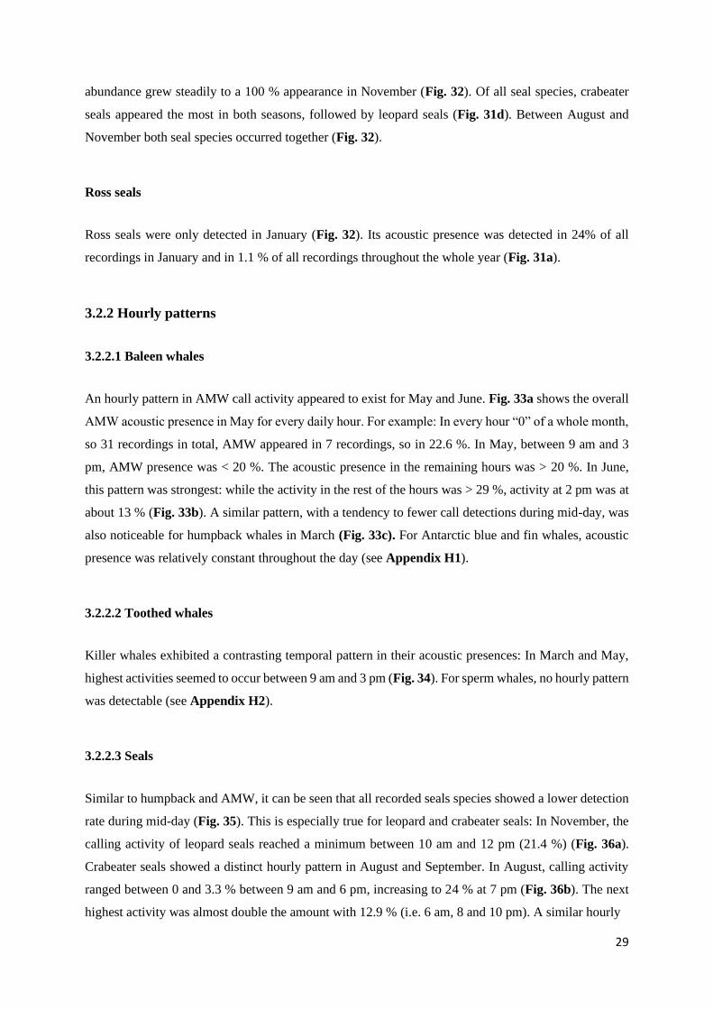
An hourly pattern in AMW call activity appeared to exist for May and June. Fig. 33a shows the overall
AMW acoustic presence in May for every daily hour. For example: In every hour “0” of a whole month,
so 31 recordings in total, AMW appeared in 7 recordings, so in 22.6 %. In May, between 9 am and 3
pm, AMW presence was < 20 %. The acoustic presence in the remaining hours was > 20 %. In June,
this pattern was strongest: while the activity in the rest of the hours was > 29 %, activity at 2 pm was at
about 13 % (Fig. 33b). A similar pattern, with a tendency to fewer call detections during mid-day, was
also noticeable for humpback whales in March (Fig. 33c). For Antarctic blue and fin whales, acoustic
presence was relatively constant throughout the day (see Appendix H1).
3.2.2.2 Toothed whales
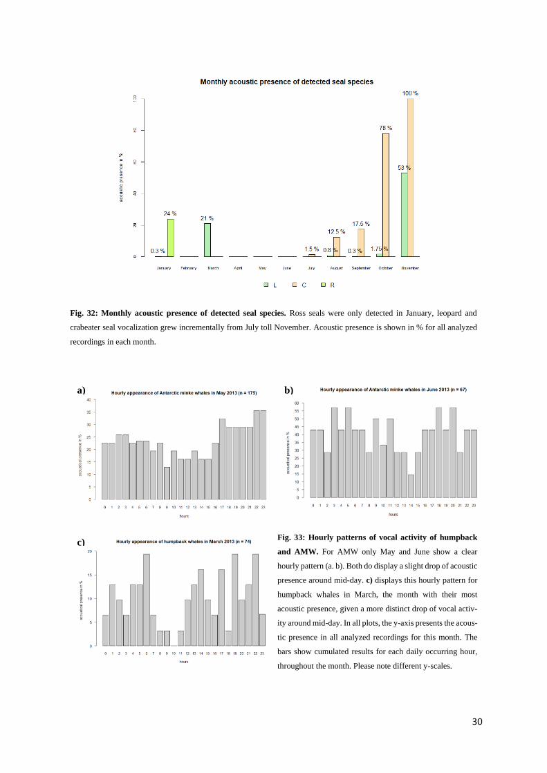
Killer whales exhibited a contrasting temporal pattern in their acoustic presences: In March and May,
highest activities seemed to occur between 9 am and 3 pm (Fig. 34). For sperm whales, no hourly pattern
was detectable (see Appendix H2).
3.2.2.3 Seals
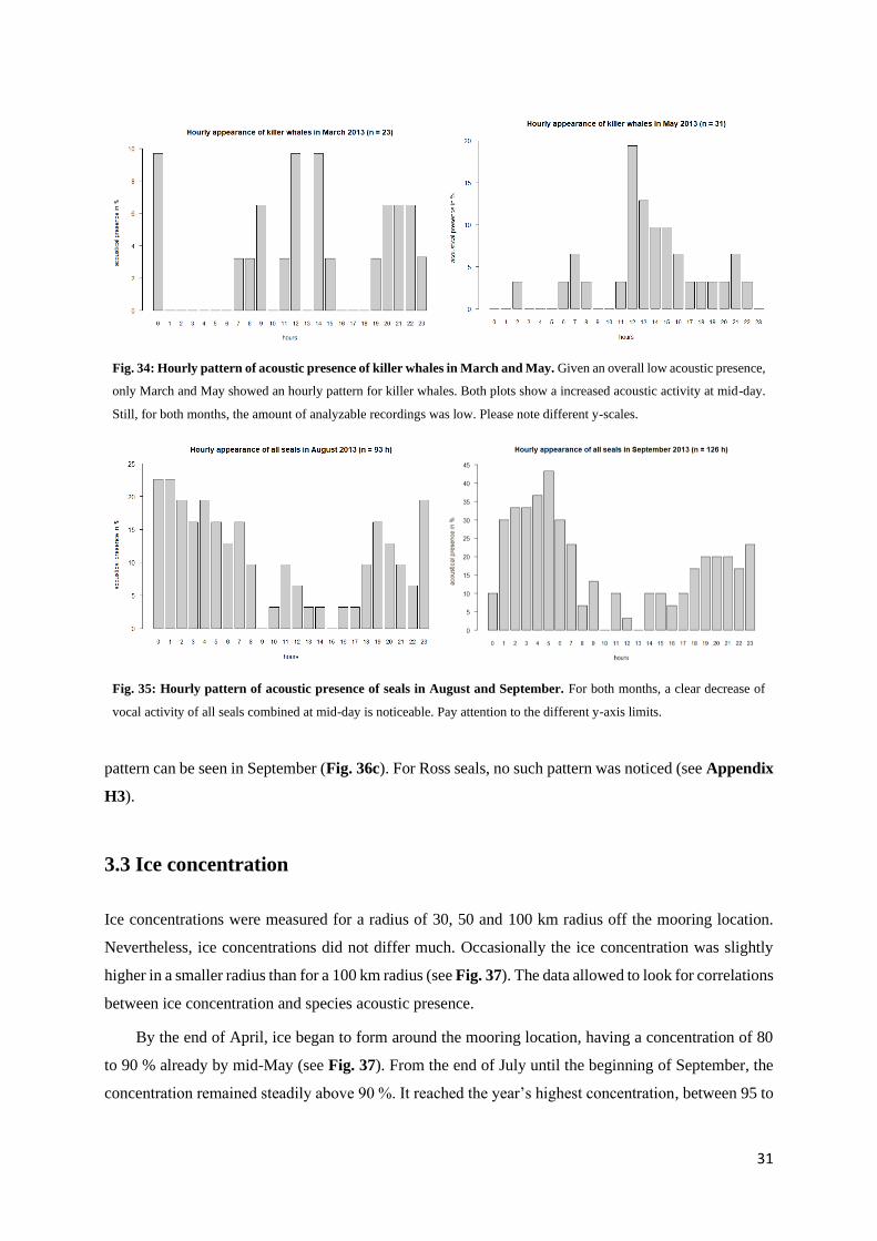
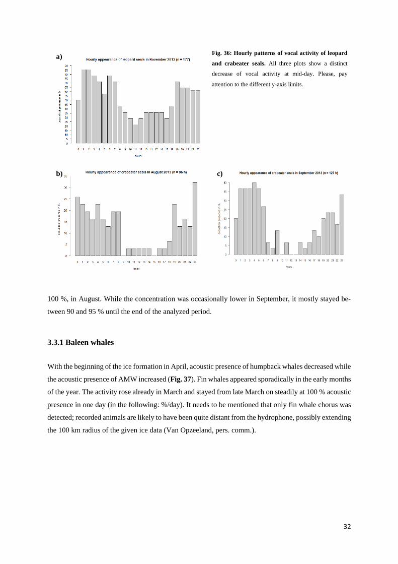
Similar to humpback and AMW, it can be seen that all recorded seals species showed a lower detection
rate during mid-day (Fig. 35). This is especially true for leopard and crabeater seals: In November, the
calling activity of leopard seals reached a minimum between 10 am and 12 pm (21.4 %) (Fig. 36a).
Crabeater seals showed a distinct hourly pattern in August and September. In August, calling activity
ranged between 0 and 3.3 % between 9 am and 6 pm, increasing to 24 % at 7 pm (Fig. 36b). The next
highest activity was almost double the amount with 12.9 % (i.e. 6 am, 8 and 10 pm). A similar hourly
30
Fig. 32: Monthly acoustic presence of detected seal species. Ross seals were only detected in January, leopard and
crabeater seal vocalization grew incrementally from July toll November. Acoustic presence is shown in % for all analyzed
recordings in each month.
Fig. 33: Hourly patterns of vocal activity of humpback
and AMW. For AMW only May and June show a clear
hourly pattern (a. b). Both do display a slight drop of acoustic
presence around mid-day. c) displays this hourly pattern for
humpback whales in March, the month with their most
acoustic presence, given a more distinct drop of vocal activ-
ity around mid-day. In all plots, the y-axis presents the acous-
tic presence in all analyzed recordings for this month. The
bars show cumulated results for each daily occurring hour,
throughout the month. Please note different y-scales.
a) b)
c)
31
pattern can be seen in September (Fig. 36c). For Ross seals, no such pattern was noticed (see Appendix
H3).
3.3 Ice concentration
Ice concentrations were measured for a radius of 30, 50 and 100 km radius off the mooring location.
Nevertheless, ice concentrations did not differ much. Occasionally the ice concentration was slightly
higher in a smaller radius than for a 100 km radius (see Fig. 37). The data allowed to look for correlations
between ice concentration and species acoustic presence.
By the end of April, ice began to form around the mooring location, having a concentration of 80
to 90 % already by mid-May (see Fig. 37). From the end of July until the beginning of September, the
concentration remained steadily above 90 %. It reached the year’s highest concentration, between 95 to
Fig. 34: Hourly pattern of acoustic presence of killer whales in March and May. Given an overall low acoustic presence,
only March and May showed an hourly pattern for killer whales. Both plots show a increased acoustic activity at mid-day.
Still, for both months, the amount of analyzable recordings was low. Please note different y-scales.
Fig. 35: Hourly pattern of acoustic presence of seals in August and September. For both months, a clear decrease of
vocal activity of all seals combined at mid-day is noticeable. Pay attention to the different y-axis limits.
32
100 %, in August. While the concentration was occasionally lower in September, it mostly stayed be-
tween 90 and 95 % until the end of the analyzed period.
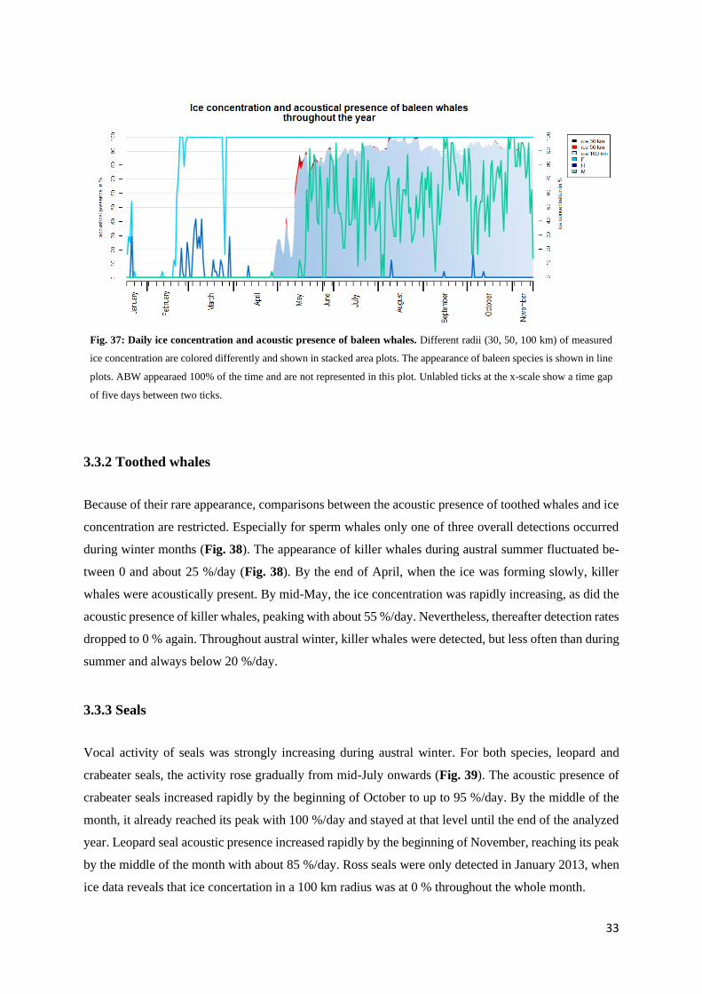
3.3.1 Baleen whales
With the beginning of the ice formation in April, acoustic presence of humpback whales decreased while
the acoustic presence of AMW increased (Fig. 37). Fin whales appeared sporadically in the early months
of the year. The activity rose already in March and stayed from late March on steadily at 100 % acoustic
presence in one day (in the following: %/day). It needs to be mentioned that only fin whale chorus was
detected; recorded animals are likely to have been quite distant from the hydrophone, possibly extending
the 100 km radius of the given ice data (Van Opzeeland, pers. comm.).
Fig. 36: Hourly patterns of vocal activity of leopard
and crabeater seals. All three plots show a distinct
decrease of vocal activity at mid-day. Please, pay
attention to the different y-axis limits.
a)
b) c)
33
Fig. 37: Daily ice concentration and acoustic presence of baleen whales. Different radii (30, 50, 100 km) of measured
ice concentration are colored differently and shown in stacked area plots. The appearance of baleen species is shown in line
plots. ABW appearaed 100% of the time and are not represented in this plot. Unlabled ticks at the x-scale show a time gap
of five days between two ticks.
3.3.2 Toothed whales
Because of their rare appearance, comparisons between the acoustic presence of toothed whales and ice
concentration are restricted. Especially for sperm whales only one of three overall detections occurred
during winter months (Fig. 38). The appearance of killer whales during austral summer fluctuated be-
tween 0 and about 25 %/day (Fig. 38). By the end of April, when the ice was forming slowly, killer
whales were acoustically present. By mid-May, the ice concentration was rapidly increasing, as did the
acoustic presence of killer whales, peaking with about 55 %/day. Nevertheless, thereafter detection rates
dropped to 0 % again. Throughout austral winter, killer whales were detected, but less often than during
summer and always below 20 %/day.
3.3.3 Seals
Vocal activity of seals was strongly increasing during austral winter. For both species, leopard and
crabeater seals, the activity rose gradually from mid-July onwards (Fig. 39). The acoustic presence of
crabeater seals increased rapidly by the beginning of October to up to 95 %/day. By the middle of the
month, it already reached its peak with 100 %/day and stayed at that level until the end of the analyzed
year. Leopard seal acoustic presence increased rapidly by the beginning of November, reaching its peak
by the middle of the month with about 85 %/day. Ross seals were only detected in January 2013, when
ice data reveals that ice concertation in a 100 km radius was at 0 % throughout the whole month.
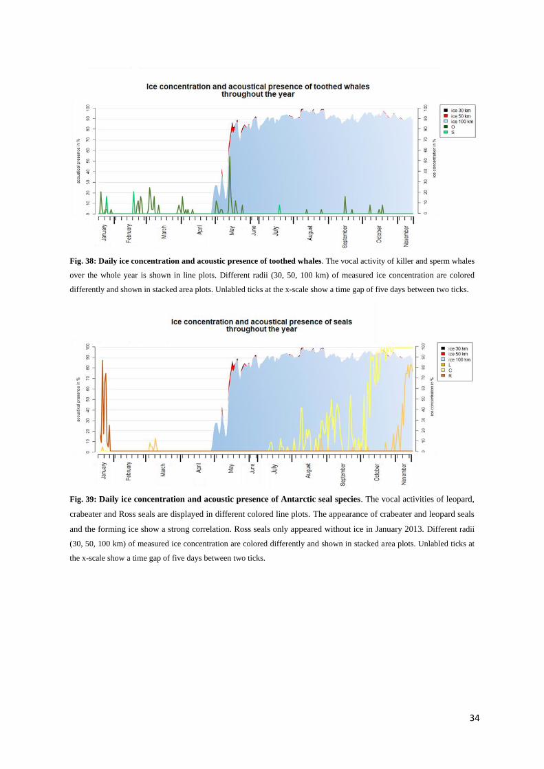
34
Fig. 39: Daily ice concentration and acoustic presence of Antarctic seal species. The vocal activities of leopard,
crabeater and Ross seals are displayed in different colored line plots. The appearance of crabeater and leopard seals
and the forming ice show a strong correlation. Ross seals only appeared without ice in January 2013. Different radii
(30, 50, 100 km) of measured ice concentration are colored differently and shown in stacked area plots. Unlabled ticks at
the x-scale show a time gap of five days between two ticks.
Fig. 38: Daily ice concentration and acoustic presence of toothed whales. The vocal activity of killer and sperm whales
over the whole year is shown in line plots. Different radii (30, 50, 100 km) of measured ice concentration are colored
differently and shown in stacked area plots. Unlabled ticks at the x-scale show a time gap of five days between two ticks.
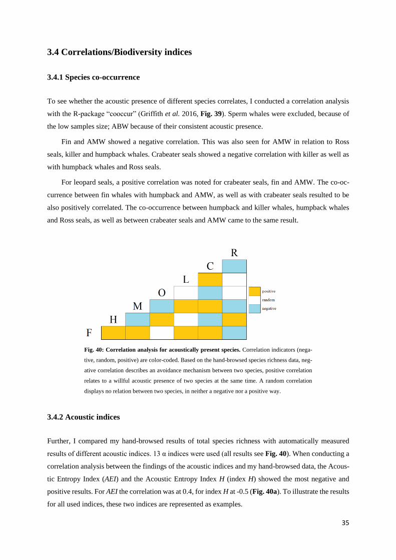
35
3.4 Correlations/Biodiversity indices
3.4.1 Species co-occurrence
To see whether the acoustic presence of different species correlates, I conducted a correlation analysis
with the R-package “cooccur” (Griffith et al. 2016, Fig. 39). Sperm whales were excluded, because of
the low samples size; ABW because of their consistent acoustic presence.
Fin and AMW showed a negative correlation. This was also seen for AMW in relation to Ross
seals, killer and humpback whales. Crabeater seals showed a negative correlation with killer as well as
with humpback whales and Ross seals.
For leopard seals, a positive correlation was noted for crabeater seals, fin and AMW. The co-oc-
currence between fin whales with humpback and AMW, as well as with crabeater seals resulted to be
also positively correlated. The co-occurrence between humpback and killer whales, humpback whales
and Ross seals, as well as between crabeater seals and AMW came to the same result.
Fig. 40: Correlation analysis for acoustically present species. Correlation indicators (nega-
tive, random, positive) are color-coded. Based on the hand-browsed species richness data, neg-
ative correlation describes an avoidance mechanism between two species, positive correlation
relates to a willful acoustic presence of two species at the same time. A random correlation
displays no relation between two species, in neither a negative nor a positive way.
3.4.2 Acoustic indices
Further, I compared my hand-browsed results of total species richness with automatically measured
results of different acoustic indices. 13 α indices were used (all results see Fig. 40). When conducting a
correlation analysis between the findings of the acoustic indices and my hand-browsed data, the Acous-
tic Entropy Index (AEI) and the Acoustic Entropy Index H (index H) showed the most negative and
positive results. For AEI the correlation was at 0.4, for index H at -0.5 (Fig. 40a). To illustrate the results
for all used indices, these two indices are represented as examples.
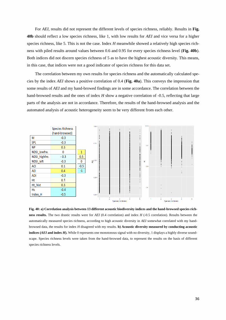
36
For AEI, results did not represent the different levels of species richness, reliably. Results in Fig.
40b should reflect a low species richness, like 1, with low results for AEI and vice versa for a higher
species richness, like 5. This is not the case. Index H meanwhile showed a relatively high species rich-
ness with piled results around values between 0.6 and 0.95 for every species richness level (Fig. 40b).
Both indices did not discern species richness of 5 as to have the highest acoustic diversity. This means,
in this case, that indices were not a good indicator of species richness for this data set.
The correlation between my own results for species richness and the automatically calculated spe-
cies by the index AEI shows a positive correlation of 0.4 (Fig. 40a). This conveys the impression that
some results of AEI and my hand-browed findings are in some accordance. The correlation between the
hand-browsed results and the ones of index H show a negative correlation of -0.5, reflecting that large
parts of the analysis are not in accordance. Therefore, the results of the hand-browsed analysis and the
automated analysis of acoustic heterogeneity seem to be very different from each other.
Fig. 40: a) Correlation analysis between 13 different acoustic biodiversity indices and the hand-browsed species rich-
ness results. The two drastic results were for AEI (0.4 correlation) and index H (-0.5 correlation). Results between the
automatically measured species richness, according to high acoustic diversity in AEI somewhat correlated with my hand-
browsed data, the results for index H disagreed with my results. b) Acoustic diversity measured by conducting acoustic
indices (AEI and index H). While 0 represents one monotonous signal with no diversity, 1 displays a highly diverse sound-
scape. Species richness levels were taken from the hand-browsed data, to represent the results on the basis of different
species richness levels.
37
4. Discussion
Most studies in the past, which observed marine mammals in the Southern Ocean using PAM, explored
the acoustic presence of one focal species. In this study, the observation site was fixed, observing all
acoustically present animals throughout ten months in 2013. I gained a deeper insight into the species
richness of marine mammals in the Antarctic, the animals’ community compositions, seasonality and
their relation to ice concentration.
In my study, as in all other studies that analyze passive acoustic data, it is important to mention that
the absence of calls does not reflect necessarily the absence of animals. In most of the detected marine
mammal species, only males conduct in vocalization and eventually only during mating season. Juve-
niles, females and not reproductively active males would otherwise be excluded. Based on this fact,
acoustic presence mostly only confirms the presence of males, the presence of further conspecifics can
only be guessed, assuming the context in which the vocalizing is used.
4.1 Baleen whales
In this study, four out of seven baleen whale species known to appear in the Southern Ocean were de-
tected. Antarctic blue, fin, humpback and AMW were acoustically present. Still, three more baleen
whale species are reported to occur in the Southern Ocean around Antarctica: southern right whales
(Eubalaena australis, Desmoulins 1822), pygmy blue whales (Balaenoptera musculus brevicauda,
Ichihara 1966) and sei whales (Balaenoptera borealis, Lesson 1828) (Lowther 2018). Most likely, they
were not detected because of their distribution, i.e. sei whales are known to mainly occur north of 60°
S, in mainly all oceans (Kato et al. 1995, Cooke 2018 (2)).
4.1.1 Migratory behavior
The four baleen whale species acoustically present in this study, except AMW (see section 4.1.5.2 for
further discussion), are known to conduct a migratory movement between high latitude summer feeding
grounds and relatively unproductive low latitude winter breeding grounds (Kellogg 1929, Corkeron &
Conner 1999). In my findings, all four detected baleen whales were also acoustically present during
austral winter, merely supports a strict separation of summer and winter grounds (Fig. 37).
In austral spring, baleen whales start to migrate from lower winter-breeding grounds to higher lat-
itudes in the Southern Ocean to feed, mostly on Antarctic krill (Euphausia superba Dana 1850, Stafford
et al. 2004, Branch et al. 2007a). In austral spring, adult krill starts migrating from their protective
inshore and under-ice habitats in austral winter to offshore waters and continental shelf areas in summer
and autumn (Nowacek et al. 2011). Therefore, in summer, high latitude waters contain a large amount

38
of krill, which is an important food source, not only for whales, but also seals, birds and fish (May 1979,
Costa & Crocker 1996, Fraser & Trivelpiece 1996). Hence, the dependence of baleen whales on krill
determines their distribution according to areas with high prey abundances (Friedlaender et al. 2006,
Santora et al. 2010).
Despite the assumption that all individuals of a population migrate together from one ground to
another, it is getting clearer that migration is not as restricted as always assumed and also differentiates
between baleen whale species (Chapman 1974). Not all individuals of one species, or even of one pop-
ulation, arrive and leave the Southern Ocean at the same time. Several studies propose that the time of
migration is more variable, as well as the decision to migrate in itself (e.g. Chittleborough 1965, Brown
et al. 1995, Acevedo et al. 2014, Thomisch et al. 2016). ABW, along with fin and humpback whales,
were already reported many times to be acoustically present throughout austral winter (e.g. Brown et al.
1995, Dawbin 1997, Širović et al. 2004, Branch et al. 2007a). This was also seen in my findings.
Širović et al. (2008) proposed that a year-round vocalization of ABW could imply a non-synchro-
nized migration of ABW or ABW populations. Dingle and Drake (2007) even proposed a partial migra-
tion of ABW between the Southern Ocean and sub-Antarctic waters. Though ABW song was not clearly
seen throughout the whole year in my study, chorus as blurring ABW song of distant animals, was still
detectable, indicating their presence in the Southern Ocean also during austral winter (Gedamke et al.
2007). Therefore, in my findings some ABW did possibly not migrate all the way north to tropical waters
but stayed in sub-Antarctic waters throughout austral winter.
In my study, humpback whales were also detected occasionally, assuming some individuals to
overwinter as well. For humpback whales, several studies proposed a sex-segregated migration or the
assumption that some individuals not take part in this energetically costly migration at all, but stay at
the feeding grounds also during austral winter (Chittleborough 1965, Dawbin 1966, Clapham 1993,
Brown 1995, Dawbin 1997, Širović et al. 2004). Brown et al. (1995) reported a sex-bias at the breeding
grounds in East Australia towards males. This was also seen in other observations (Craig & Herman
1997, Pomilla & Rosenbaum 2006). Females that were reported at the breeding grounds during austral
winter were mostly lactating (Lockyer & Brown 1981, Brown et al. 1995). Therefore, humpback whales
that were observed visually and acoustically to overwinter at the feeding grounds are thought to be
mostly females, which are either not yet fecund or not lactating (Brown et al. 1995). Since for whales it
is assumed that not the age decides on the fecundity, but size and weight, it is possible that juveniles or
immature or poor condition females, stay at the feeding grounds during winter, gaining weight for a
reproductive advantage by maximizing their growth (Chittleborough 1965, Lockyer 1984, Brown et al.
1995).
Approximately a quarter of the yearly energy budgets for female adult Antarctic blue and fin whales
is utilized during migration, assuming 15 days of continuous swimming (Lavigne et al. 1990). The mi-
gration of humpbacks is reported to be even further, therefore, they consume more energy in comparison
39
to other migratory whales (Stone et al. 1990). This might not be profitable for some females (Lockyer
1984).
Though food resources are smaller than in austral summer and harder to reach because of the ice
cover, there are also less food competitors (Brown et al. 1995). Baleen whales are mostly reported to
stay north of the pack ice, at the ice edge zone, which is reportedly a high productive zone during winter
month, offering a reliable amount of food (Hempel 1985, Knox 2007 (2), Van Opzeeland et al. 2013
(2)). These assumptions go in hand with my findings that detected baleen whales were probably far
away from the recorder during austral winter, given their distant vocalization.
The belief that females overwinter can be supported by the fact that, i.e. ABW and humpback whale
song, solemnly produced by males in a mating context, was detected during austral winter (Brown et al.
1995, Simon et al. 2010, Thomisch et al. 2016). Hence, males are assumed to benefit from overwinter-
ing, by rising their reproduction possibilities.
Nevertheless, the cold water in the Southern Ocean could also be presumed to be a stressor during
austral winter. Lavigne et al. (1990) calculated potential energy levels in different scenarios and found
that baleen whales cannot conserve energy from migrating from cold to warm water, further that the
energy that it costs to bear the coldness is not as high as presumed. Still, an important benefit of migrat-
ing to lower latitudes during austral winter would be to avoid a high predatory pressure of killer whales
and the rough unsteady ocean during austral winter (Corkeron & Conner 1999, Longhurst 2007). In
addition, there is always a risk for surface-breathing marine mammals to be trapped under the ice cover
or in polynyas without escape (e.g. Porsild 1918, Taylor 1957).
4.1.2 Hourly patterns
For some species, hourly patterns in different months were noticeable, resulting supposedly from prey-
ing behavior.
Most detected species showed an increased acoustic presence during the night (compare with Fig.
33a, 35, 36, Seibert et al. 2007, Thomas & Rogers 2009a, Van Opzeeland et al. 2010). These findings
most likely go back to a diel vertical movement of krill, migrating to the surface during the night (e.g.
Taki et al. 2005, Gaten et al. 2008, Wiebe et al. 2011). As Antarctic krill is the main food source for
many marine mammals in the Southern Ocean, surface feeder like humpback and AMW or crabeater
seals use the surfacing movement of krill, to forage during the night (Lascara et al. 1999, Nicol 2006,
Lawson et al. 2008, Novacek 2011). With krill migrating to deeper water during the day, vocal activity
of krill-feeding species decreases. Novacek (2011) even explains a decrease of humpback whale vocal
activity by a resting behavior during the day.
An hourly pattern according to krill’s diel movement does not only occur for krill-eating marine
mammals alone: For example, cephalopods and fish, feeding on krill also follow its diel movement,
40
resulting in an hourly pattern for marine mammals preying on cephalopods and fish, like Ross seals
(Ray 1981, Southwell et al. 2012). Nevertheless, because of the small sample size, no hourly pattern
was noticed for Ross seals (see Appendix H). A diel pattern for leopard seals is also indirectly based
on krill: Leopard seals feed on seal pups of other species. They encounter them during the night, as they
forage on krill (Siniff & Stone 1985, Borsa 1990, Walker et al. 1998, Hiruki-Raring 1999).
For seals, a decrease of acoustic presence at mid-day is also based on a haul out behavior onto the
ice to sunbath (Fig. 35). According to Williams (2003) in early austral spring, when sunlight emerges
slowly after a dark cold winter, Weddell seals have been reported to start sunbathing on the ice during
mid-day, finally warming up again. This haul out behavior is also documented for other Antarctic seal
species (e.g. Bengtson & Stewart 1997, Southwell 2003).
For killer whales, an increased acoustic presence at mid-day was detectable in March and May (Fig.
34). Miller et al. (2010) suggest a diel movement of killer whales according to their primary prey. How-
ever, it is unclear what food source the recorded killer whales are preying on, why a reliable association
to a certain ecotype is not possible (see section 4.2.1.2).
Antarctic blue and sperm whales, did not show hourly patterns in my study (see Appendix H).
Since ABW occurred continuously and sperm whale rarely, it is not possible to detect hourly patterns
for both species. Sperm whales are deep-sea feeder, preying on krill-feeding squid (Nemoto et al. 1988,
Hooker 2001). An increased acoustic presence could therefore be expected during the day, when squid
follow the krill’s diel movement to deeper water. Further, there was no reliable hourly pattern found for
fin whales (see Appendix H). Still, sufficient data was only available from mid-January until mid-
March, after this period fin whale vocalization was detected continuously. Fin whales are known to feed
on Antarctic krill species, as well as small fish, why an increased acoustic presence at night would be
expected (e.g. Mizroch et al. 1984, Burkhardt & Lanfredi 2012, Nøttestad & Olsen 2004). An according
pattern can be surmised for January, but not for the remaining data.
4.1.2 Antarctic blue whales
In my results, characteristic ABW song (Z-calls) and chorus were detected (Fig. 3, Ljungblad et al.
1998, Rankin et al. 2005. McDonald et al. 2006a, Branch et al. 2007, Gedamke et al. 2007).
These high intensity low frequency calls are known to transmit very far in water (e.g. Cumming &
Thompson 1971, Payne & Webb 1971, Stafford et al. 1998, Širović et al. 2007). Being able to emit calls
that can be heard over a long distance is extremely important for the survival of a population, when it is
highly depleted and conspecifics are far away (Payne & Webb 1971).
Song was detected all year round with a peak, noticed by distinct Z-calls, between January and
March. Similar results were found by several other studies conducted at different locations in the South-
ern Ocean (e.g. Širović et al. 2008, Miller et al. 2015, Thomisch et al. 2016). Chorus was detected
41
throughout the rest of the year, arising when many distant animals sing. In this case, the upper compo-
nent melts together into a continuous line, actually consisting of multiple Z-calls produced by animals
at different distances from the receiver (Gedamke et al. 2007). The year-round recording of ABW indi-
cates a variable migratory behavior with individuals overwintering in the Southern Ocean (compare with
section 4.1.1, Mackintosh & Wheeler 1929, Harmer 1931, Hjort et al. 1932).
Song is known to be produced in a mating, feeding and also migratory context produced by solitary
males (McDonald et al. 2001, Croll et al. 2002, Oleson et al. 2007, Širović et al. 2009, Širović & Hil-
debrand 2011). It can therefore be estimated that besides vocalizing males also female ABW were pre-
sent during the recorded austral winter.
Compared to humpback whales, which use song prior mating, the continuous calling of male ABW
are difficult to put into this stereotyped display. It is known that the main mating season for ABW is in
late autumn (approx. July) with a gestation period of 10-12 months (Shirihai 2006). Though Clark and
Clapham (2004) proposed that the continuous vocalization leads to believe that mating is not limited to
a certain season or habitat, there are no aseasonal births documented to date, which would be the case
for year-round mating. Therefore, continuous ABW song is unlikely leading directly to mating (Oleson
et al. 2007a). Oleson et al. (2007 a) proposed that a continuous vocalization might demonstrates the
male’s endurance and fitness, like a long-term assessment and following association to a female prior
to mating in more temperate waters.
4.1.3 Fin whales
Fin whales were, despite their common seasonal migratory behavior, detected year-round in this
study (Joiris & Dochy 2013, Bannister & Adamczak 2018, Van Opzeeland & Hillebrand, submitted).
My results even show a higher acoustic presence for fin whales in winter, then during summer months,
which is commonly known for AMW, but for fin whales this reversed appearance is unusual (e.g. Ribic
et al. 1991; Thiele et al. 2004, Dominello & Širović 2016, see 4.1.5.2 for discussion of AMW findings).
Fin whales areknown to inhabit open pelagic waters, far away from the coast (Shirihai 2016). Širo-
vić et al. (2004) even observed fin whales directly avoiding ice covered areas. Still, krill abundance is
especially high in areas of large sea ice fluctuation (Smith & Nelson 1985, Loeb et al. 1997, Nicol et al.
2000). A strongly retreated ice cover therefore does not provide many resources, which could explain
the low acoustic presence in January and February of fin whales in my study. Slowly forming ice then
attracts krill-feeding baleen whales, which can be seen by an increased acoustic presence in March. In
addition, the drop of vocal activity in March at two days could mirror the fluctuating character of form-
ing ice at the offset of austral winter.
Many studies recorded fin whale pulses year-round, also during austral winter, as in my findings.
Simon et al. (2010) even observed peaking of fin whale song, known to be used in a mating and feeding
42
context, solemnly produced by males, also during Arctic winter (e.g. Watkins et al. 1987, Thompson et
al. 1992, Thomson & Richardson 1995, Moore et al. 1998). Though to date no mating of fin whales is
documented, Lockyer (1984) estimated a peak in singing might imply the peak of conception time. This
would indicate firstly that males and females are overwintering and secondly that mating does not
merely take place at lower latitudes during winter, but could already happen before or during migration
at high latitudes (Simon et al. 2010). This assumption could be transferable for fin whale populations of
the Southern Hemisphere.
In my study, recorded song during austral winter was emitted by distant fin whales. Blurring bands
in my recordings indicate that the emitting fin whales were far away from the recorder. This goes in
hand with the observation of Van Opzeeland and Hillebrand (submitted) of baleen whales aggregating
north of the ice cover, close to the highly productive ice edge zone. Further, it complies with fin whales
reported to actively avoid ice covered areas (Širović et al. 2004).
4.1.4 Humpback whales
4.1.4.1 Calls
Humpback whale calls in my recordings contained diverse social sounds, as well as song, during
summer and winter months (see Appendix F2).
Various social sounds, like moans, grunts and unstructured high calls, are produced by males and
females and can generally be heard at feeding and breeding grounds (Silber 1986, Thompson et al. 1986,
Dunlop et al. 2007). They are thought to play a role in many social interactions like feeding, inter- and
intra-sexual social interactions and migration (Jurasz & Jurasz 1979, Tyack & Whitehead 1983, D`Vin-
cent et al. 1985, Silber 1986, Dunlop et al. 2007, Dunlop et al. 2008).
The stereotyped highly structured song of humpback whales (Fig. 11) can be recognized by its
composition of phrases and themes, which, by repetition and certain assembly, built a song (Payne &
McVay 1971). It is produced by males during migration, as well as on feeding and breeding grounds,
serving in a mating context to attract females and acoustically compete with rivalling males (Payne &
McVay 1971, Clapham 2000, Darling & Bérubé 2001, Darling & SousaLima 2005). Unlike other baleen
whales, such as ABW, it is known that the mating display of male humpback whales through song is
performed right before mating (Oleson et al. 2007a).
4.1.4.2 Acoustic presence
Humpback whales were occasionally acoustically present throughout the whole year, also during austral
winter, peaking at the beginning of March, when no ice was detectable in a 100 km radius (Fig. 37, see
43
Appendix F2). In a study, observing recordings of the PerenniAL Acoustic Observatory in the Antarctic
Ocean (PALAOA, 70° 31’ S, 8° 13’ W), close to the Ekström ice shelf edge, humpbacks had been
present in 2008 and 2009 almost throughout the whole year, except September, with the highest occur-
rence between February and May (Van Opzeeland et al. 2013 (2)). These results go in hand with my
findings. The highest presence of humpback whales social sounds was observed in March, but the main
acoustic presence stretched from mid-January until mid-April (see Appendix F2). High rates of social
sounds are most likely linked to krill stock size peaking at the same time (Jurasz & Jurasz 1979, Murase
et al. 2002, Knox 2007 (2), Novacek et al. 2011).
Sporadic recordings of social sounds during austral summer, indicate animals in small distances,
probably due to travels within feeding grounds. During austral summer, long distant travels of humpback
whales are reported within their feeding ground (Dalla-Rosa 2008). It is known that at least along the
Western Antarctic Peninsula (WAP) it is part of their foraging strategy to travel short as well as exten-
sive distances from one feeding ground to another with relatively short residency times, depending on
sea ice, primary productivity and krill abundance (Dalla-Rosa 2008). This is also confirmed by Van
Opzeeland et al. (2013 (2)) who assumed that humpback whales do not have only one feeding ground
but move in longitudinal regions that animals range in a southbound direction while foraging.
Beside a high occurrence of social sounds, also the appearance of song in March indicates a high
abundance of humpback whales foraging on krill stocks. An elevated number of conspecifics promises
a raised potential for reproduction. In my findings, song was only recorded once over a relatively short
time during the year. It is also not recorded completely, given that the recoded song started and ended
in the middle of a phrase. This could go back to the high frequencies in which song is produced, not
getting transported over long distances. Further, this goes in hand with the formerly described foraging
movement that the singing humpback whale might traveled out of the recording range. Since no overlaps
of song were noticed in my recordings, it can be assumed that the analyzed song was only emitted by
one male (Payne & McVay 1971). Nevertheless, some echoes were detected during song, which could
also indicate other males singing in further distance and in a shifted manner (see Appendix J2). If
recorded echoes were other song emitting humpback whale males, it shows the affiliation of the singing
males to one population, given that males in one population are known to sing the same song (Payne et
al. 1983, Payne & Payne 1985).
Further, given the time of the year, song could indicate a migration movement towards lower lati-
tudes before the onset of austral winter (Payne & McVay 1971).
A former study took a closer look at the vocal biodiversity off Elephant Island at the WAP (61° 7′
S, 55° 11′ W) in September 2013 (Hots, unpublished). Though it is known that the ice dispersion in the
Antarctic is at its maximum in September, the vocal activity of humpback whales laid at 43% (in fre-
quency ranges of 2.5 and 16 kHz). Since also song, beside social sounds, was detectable in that study,
44
the presence of female and male humpback whales during austral winter could be assumed. This sup-
ports the formerly mentioned sex-bias towards females in the Southern Ocean, which possibly attracts
more males to overwinter as well (Brown et al. 1995, Van Opzeeland et al. 2013 (2)).
4.1.5 Antarctic minke whales
4.1.5.1 Calls
AMW pulses trains, as well as “bio-duck” calls were detected almost exclusively during austral winter
(see Appendix F3). Beside the stereotyped intense low-frequency grunt like pulse train, AMW also
produced a four-pulse sound, the so-called “bio-duck” sound, which, only recently, was reliably allo-
cated to AMW, after being a mystery for decades (Schevill & Watkins 1972, Winn & Perkins 1976,
Mellinger et al. 2000, Risch et al. 2014). Former studies detected the call between April and December,
the period between ice forming and retreating in the Southern Ocean (e.g. McCauley et al. 2004, Klinck
& Burkhardt 2008). This is in line with my findings.
Today it is known that the “bio-duck” call also underlies geographical varieties: In the Weddell Sea
the call exists of four short pulses, as seen in my recordings, while it is shortened to three pulses in the
Eastern Antarctic (Risch et al. 2014). All AMW vocalizations have in common that they occur in bouts,
over many hours, but to date not much is known about the context in which it is used.
4.1.5.2 Acoustic presence
When it comes to the distribution of AMW, very little is known. Just like all baleen whales, they are
thought to undertake a seasonal migration (Glover et al. 2010). This is encouraged by sighting data
which reported a southbound movement of AMW from lower latitudes (10-20° S) starting in October
and being present at their feeding ground in the Antarctic in January (Kasamatsu et al. 1995). It is
thought that AMW stay in offshore waters before they migrate south and distribute prey dependent and
in association with forming ice in April (Van Opzeeland 2010). This could be adopted to my findings,
in which AMW were first detected by the end of April, but were then seen throughout austral winter,
when ice concentration in a 100 km radius was mostly > 80 % (Fig. 37). For AMW, there was also a
strong sex segregated migration observed, which dissolves in sex segregated feeding grounds, with fe-
males feeding in coastal waters while males stay in offshore grounds (Kasamatsu & Ohsumi 1981, Risch
2019). Compared to my findings, it is possible that detected vocalization in my study is emitted by
female AMW.
45
AMW prey on high under-ice krill resources during austral winter (Marschall 1988, Ribic et al.
1991, Friedlaender et al. 2014). They have a strengthened rostrum, which allows them to create breath-
ing holes in dense ice cover, essential for surface-breathing marine mammals (compare with Scheidat et
al. 2008, Tynan et al. 2010). Further, they have been documented using polynyas, areas of open water
in the ice cover close to the sea-ice coast, known to form by strong winds and iceberg movements, to
surface (Comiso & Gordon 1987, Ribic et al. 1991, Dayton et al. 1994). Beside the opportunity to sur-
face, polynyas are also known to be areas with high nutrient levels and enhanced productivity (Comiso
& Gordon 1987, Dayton et al. 1994).
Adaptations, like the strengthened rostrum and their small size, give them an advantage before
larger baleen whales during austral winter to prey on under-ice krill stocks, which is not given during
austral summer, when competing for krill with top predators like large baleen whales. Though krill
stocks are depleted at the offset of austral winter, it is known that AMW populations that overwinter in
the Antarctic (> 60° S) still consume about 35.5 × 10⁶ t of krill annually (Armstrong & Siegfried 1991).
4.1.6 FM-calls
In my study, FM-calls were detected regularly between January and March and once in June and July,
respectively. FM-calls (or “D-calls”, “contact calls” or “downsweep” as called in former studies) are
produced by many baleen whales and both sexes, a reliable allocation to a certain baleen species is
therefore not possible (Watkins 1981 Ljungblad et al. 1997, McDonald et al. 2001, Rankin et al. 2005,
Dominello & Širović 2016). Still, the detection implement a presence close to the recorder, given that
FM-calls do not travel as far as song or chorus.
Calls of Northern Hemisphere populations of baleen whales, similar to FM-calls of the Southern
Hemisphere, are thought to maintain contact between conspecifics during foraging dives and general
social interactions (McDonald et al. 2001, Oleson et al. 2007). During austral winter, this would reveal
foraging of baleen whales in a small radius to the location, implying reliable food sources and access to
open water (Thomisch et al. 2016).
4.2 Toothed whales
In this study, two out of seven toothed whale species known to appear in the Southern Ocean were
detected. Killer and sperm whales appeared occasionally throughout the whole year. Five more toothed
whale species are reported to appear in the Southern Ocean: Hourglass dolphin (Lagenorhynchus cru-
ciger, Quoy & Gaimard 1824), long-finned pilot whale (Globicephala melas, Traill 1809), Arnoux’s
beaked whale (berardius arnuxii, Duvernoy 1851), southern bottlenose whale (Hyperodon planifrons,
Flower 1882) and strap toothed whale (Mesoplodon layardii, Gray 1865) (Lowther 2018). This, just as
46
for sei whales, goes back to their distribution: i.e. hourglass dolphins, long-finned pilot whales and strap
toothed whales are known to appear in the Southern Ocean but in lower latitudes that it would not have
been possible to record their vocalization (Shirihai 2006, Taylor et al. 2008, Braulik 2018, Minton et al.
2018).
4.2.1 Killer whales
4.2.1.1 Calls
Killer whale sounds were rarely detected, with most calls during austral summer. Since their various
sounds, like clicks, whistles and pulsed calls, can easily extend the recorded frequency range of 2.5 kHz
and even go up to 85 kHz, undetected sounds do not necessarily show an absence of killer whales (Dierks
et al. 1973, Ford 1989). This can also be seen in a former study: when comparing data of two recorders
moored to the same location, with two different frequency ranges (2.5 kHz and 16 kHz), killer whales
were 11% more detected with a range of 16 kHz than with 2.5 kHz (Hots, unpublished).
Killer whales are known to be highly social animals, which can be seen in overlapping calls of an
unknown number of killer whales (see Appendix J1, Janik & Slater 1997, Tyack 2008). Since only
pulsed calls were recorded, foraging or travelling can be assumed (Ford 1989).
Unlike other recorded whales species it is known that males and females are sound emitting, which
makes differentiating between vocalizing sex impossible (Ford 1989).
As high-frequency calls do not get transmitted as far as low-frequency sounds in water, it can be
supposed that sound emitting killer whales were close to the hydrophone when calls were recorded (e.g.
Cumming & Thompson 1971, Payne & Webb 1971, Stafford et al. 1998, Širović et al. 2007).
4.2.1.2 Acoustic presence
For the recorded killer whale sounds no seasonality was detected, which might indicates the presence of
different ecotypes (see Appendix I). For killer whales, it is known that different ecotypes occur in the
Northern Hemisphere (e.g. Turrill 1946, Foote et al. 2009, Riesch et al. 2012). They differ in their food
specialization, morphology and display (Pitman et al. 2010, Deecke et al. 2011, Riesch et al. 2012).
Nevertheless, different ecotypes of killer whales are also known to occur in the Southern Hemisphere.
To date five different ecotypes have been described, four of them occurring > 60 ° S (Type A-C, Pitman
& Ensor 2003, Pitman et al. 2011, Durban et al. 2016, see Appendix). The scattered vocal activity of
killer whale vocalization found throughout the analyzed year could be an indicator for different ecotype
with different food preferences (Deecke et al. 2011, Riesch et al. 2012). While an ecotype feeding on
migratory whales would be expected to be more acoustically present during austral summer, ecotypes
47
feeding on seals or AMW, would be expected to be more acoustically present during austral winter
(Pitman et al. 2001, Pitman et al. 2007). A rising abundance of baleen whales during austral winter
might also attract more whale eating killer whales. However, a distinction between different ecotypes
was not possible in my study.
Killer whale acoustic presence peaked at the beginning of May, which might be explained by the
rapidly forming ice and increase of krill and krill-feeding animals close to the ice edge zone. As already
explained could the forming ice lead to an increase in primary production at the offset of winter (see
introduction). Though there is no killer whale ecotype known in the Southern Hemisphere feeding on
krill, killer whales could be preying on krill-feeding animals like fish or marine mammals.
Since pulsed calls are thought to be used in a social context, especially during foraging and traveling,
a forming ice cover and a prolonged night at the beginning of austral winter could make vocalization
also more important to communicate with conspecifics (Ford 1989).
The only occasionally recorded killer whale sounds could be explained by their fast agile swimming
behavior. Since they are fast swimmer, recorded vocalization could indicate only a passing (e.g. Fish
1998, 2002).
4.2.2 Sperm whales
4.2.2.1 Acoustic presence
This study shows that sperm whales occurred rather patchily throughout the recording period. Only
usual clicks, thought to be used during deep dives for echolocating and foraging, were detected on three
not continuous days over the whole year (see Appendix G, Verboom 1998, Hooker 2001, Whitehead
2009). The days were spread over two days during summer and one day during winter months. When
Van Opzeeland and Hillebrand (submitted) compared eight years of recordings of the Southern Ocean,
detections of sperm whales were not mentioned at all, assuming no or very rare encounters, being in line
with my findings.
Usual clicks in austral winter indicate sperm whales foraging. Adult male sperm whales are known
to follow the migration of their prey to latitudes higher than 60° S during austral summer, including fish,
sharks and cephalopods (Verboom 1998, Whitehead 2003). Nevertheless, the recorded encounter during
austral winter is unusual, given the fact, that sperm whales are reported to avoid ice (Hooker 2001). In
July, when clicks were detected in my study, the ice cover in a 100 km radius was above 80 %. There
have been reports of occasional detections in March, April, May and November, but to my knowledge
never in months with solid ice cover (Hooker 2001). In addition, recorded usual clicks of sperm whales
are of high frequency, which indicates that animals were even relatively close to the hydrophone (about
10-20 km, e.g. Walker et al. 2003, Barlow & Taylor 2005).
48
4.3 Seals
In this study, I was able to detect three out of six seal species that are known to occur in the Southern
Ocean and to produce underwater vocalization. I detected leopard, crabeater and Ross seals but was not
able to detect Weddell (Leptonychotes weddellii Lesson 1826), Antarctic fur (Arctocephalus gazelle
Peters 1875) and southern elephant seals (Mirounga leonine Linnaeus 1758) in my recordings (Lowther
2018). Antarctic fur seals do not appear below 60° S, therefore a detection was not possible (Shirihai
2006, Hofmyer 2016). Weddell seals are usually detected in the Weddell Sea (> 60 ° S) and stay pref-
erably inshore (Hückstädt 2015 (2)). Acoustic presence has been recorded also incidentally for offshore
sites like the one analyzed here, but are less common than in areas closer to the ice shelf.
4.3.1 Seasonal behavior
Not much is known about Antarctic seals, especially about the mating and breeding behavior given that
it is conducted underwater, mainly in darkness during austral winter and mostly too far from any re-
search station.
In my study, calls of the three detected ice-breeding seals were seen as soon as ice formed and peaked
in October and November, marking the breeding and mating season. All three detected seal species show
a strong relation to ice (Van Opzeeland 2010). Single calls of leopard and crabeater seals can already be
heard at the beginning of austral winter, showing an incremental migration along with the forming ice
northwards (Fig. 39, 32, e.g. Walker et al. 1998, Nordoy & Blix 2002, Forcada & Robinson 2006).
It is known that pupping of ice-breeding seals happens late winter early spring within the pack ice.
At that time, ice floes provide numerous opportunities for pupping and nursing in an area of high food
supply and unrestricted access to water (Rogers et al. 1996). Peaking snow accumulation and tempera-
tures well below freezing are necessary to ensures that the icy underground is stable, minimizing the
risk of mortality because of ice breakup (Pierotti & Pierotti 1980, Bester et al. 1995, Southwell et al.
2003b, Southwell et al. 2004, Van Opzeeland et al. 2010). If the ice is not thick enough, expecting seal
cows risk that pups break into the ice, being captured by waiting predators, like killer whales or leopard
seals (Pierotti and Pierotti 1980). For Ross seals, pupping occurs commonly in November, which was
not analyzed in this study (Blix & Nordoy 2007). In general, optimal conditions for foraging and breed-
ing are only available over a short period, seasonal behavior like pupping and breeding is therefore
synchronized in ice breeding seal species (Van Opzeeland 2010).
The mating season is marked by peaking underwater vocalization. For leopards and crabeater seals
this peaking can be seen by the end of October and November in my study. All three detected seal
species are semi-aquatic and pursue aquatic mating, for which underwater vocalization is especially
important, given the dispersal of conspecifics and the low visual quality (Lydersen & Kovacs 1999, Van
49
Opzeeland et al. 2010). Underwater vocalization of crabeater seals is only emitted by males, used during
foraging on krill and fish to call conspecifics to found food resources. They can also be part of a mating
display, especially attracting females to food resources or in male-male-competitions (Oritsland 1977,
Siniff et al. 2008, Van Opzeeland et al. 2010). For leopard seals, both sexes are able to vocalize and use
their calls over long distances in a mating context (Shaughnessy & Kerry 1989, Rogers et al. 1996).
Nevertheless, it is important to mention, that detected seal species inhabit different ecological
niches: For example, the foraging, mating and breeding behavior and the preferred ice type used for
breeding differ (Van Parijs et al. 2004, Siniff et al. 2008, Van Opzeeland et al. 2010).
4.3.2.2 Juvenile leopard seal calls
In March, some incomplete calls of juvenile leopard seals were detected (Fig. 21, Rounsevell &
Pemberton 1994, Rogers et al. 2005, Rogers 2007). While most Antarctic seals, also adult leopard seals,
are thought to stay at near-shore areas, the dispersal of juvenile leopard seals in austral summer also in
offshore waters (as seen in my recordings) is proposed to be related to resources like mates or food
which are spread out further north (Dobson 1982). The isolated peaking vocalization appeared simulta-
neously with the peak of humpback whale calls in March 2013 and could therefore indicate a northbound
dispersal of juveniles because of a food incidence. Nevertheless, Van Opzeeland (2010) reported also
juvenile calls near the PALAOA station. This suggests that the juvenile dispersal is not only limited to
northern waters.
4.3.2 Ross seals
Beside other Antarctic seal species, little is known about Ross seals, but it is assumed that they are the
least abundant seal species in the Antarctic (e.g. Scheffer 1958, Reeves et al. 1992, Thomas & Rogers
2009).
In my study, Ross seal underwater vocalizations was detected exclusively in January (Fig. 32). The
typical calls of Ross seals cannot be confused with any other vocalization, because of its characteristic
siren-like sounds (Seibert et al. 2007). Overall, they emit five different types of calls, of which only mid
and high siren calls were detected (Van Opzeeland et al. 2010). Long-ranged underwater calls are as-
sumed to be used in male-male-competitions as well as in mating purposes, with calls peaking between
December and February (Watkins et al. 1985, Stacey 2006, Van Opzeeland 2010, Van Opzeeland &
Hillebrand, submitted).
For Ross seals, certain phases and distribution over seasons are known. Blix and Nordoy (2007)
documented that pupping of Ross seals takes place in November, followed by a short breeding and
mating period, resolving in a peaking vocalization. This cannot be seen in my study, which is also due
50
to the fact that recordings were only analyzed till mid-November. After, females are reported to head
north in open waters by the end of November and return by early/mid-January to the pack ice, while
males and barren females stay in the pack ice the entire time (Blix & Nordoy 2007). In my study, high
acoustic presence during January could indicate the return of these formerly pelagic females, though it
needs to be noticed that only male Ross seals are thought to vocalize (e.g. Rogers 2003, Van Opzeeland
et al. 2010). In this time, from mid-January until mid-February, a short period of moulting is reported,
in which animals form large aggregations on ice floes (Skinner & Klages 1994, Blix & Nordoy 2007,
Thomas & Rogers 2009). This is followed by Ross seals heading far north, mostly right before the polar
front, into open water, to spend several months (until November) in a pelagic phase to feed (Blix &
Nordoy 2007). This northbound migration in February can be noticed by the sudden drop of Ross seal
calls end of January (Fig. 39). Similar results were found in other studies (e.g. Blix & Nordoy 2007,
Seibert et al. 2007).
Unlike leopard seals, for Ross seals it proposed that their appearance is associated with certain ice
features like pack ice density. This is assumed since the peak of the vocalization and the peak of the
pack ice density were observed to occur at the same time (Van Opzeeland et al. 2010). This cannot be
seen in my results. In January, when vocalization of Ross seals occurrred, there was no ice cover notice-
able in a 100 km radius (Fig. 39). Nevertheless, acoustic and ice data between mid-November until mid-
January are missing, leaving a gap to confirm this coherence in my study.
4.3.3 Weddell seals
The fourth underwater vocalizing seal, the Weddell seal, was recorded close to the coast, near PALAOA
year-round (Van Opzeeland et al. 2010). In my analyzed data, no Weddell seal vocalization was de-
tected. This could show that while other seals travel northbound with the forming ice, Weddell seals
stay at their occupied territory. They are known to not be migratory but travel short distances to breathing
holes and exit cracks during austral winter (Stirling 1969, Hückstädt 2015 (2)). This mainly philopatric
behavior might gives an advantage, being accepted in their habitat as dominant.
51
4.4 Other sounds
Besides biotic vocalization, many other sounds have been recorded. The shown sounds in the following
part appeared more than once, regularly or over a longer time span, but could not be assigned to a sound
emitting source.
4.4.1 Unidentified toothed whale
The stereotyped toothed whale click train with a very high repetition rate over a short time was only
audible at two occasions in my analysis. The unknown clicks appeared in August and September. In a
former study of Meister (2017) passive acoustic data of Elephant Island between 2013 and 2016 was
analyzed. The recordings contained comparable click trains. throughout all years: In 2013 and 2014, the
clicks appeared in August, between 2013 and 2015 they also appeared in September (Meister 2017).
What is very unusual is the low frequency of below 2.5 kHz, in which the click train appeared (Fig. 27).
Toothed whales like beaked whales or dolphins are known to produce clicks and other vocalization
which extended the here used 2.5 kHz (e.g. Dierks et al. 1973, Zimmer et al. 2005, Johnson et al. 2006,
Reyes Reyes et al. 2015). While the unknown click train was recorded, Antarctic blue, fin and AMW
were present. To my knowledge, there is no documentation of sounds produces by these species com-
parabale to the found click train. Nevertheless, the vocal repertoire of the five different killer whale
ecotypes of the Southern Ocean are not yet investigated fully (Pitman et al. 2001, Pitman & Ensor 2003,
Durban et al. 2016, Schall & Van Opzeeland 2017). Further, the unknown clicks cannot be associated
to ice appearances, since it appeared irregularly in months with and without ice (Meister 2017).
As mentioned in section 4.2, former studies detected other toothed whale species in the Southern
Ocean that I was not able to hear, like long-finned pilot whales, southern bottlenose whales and strapped-
toothed whales (Lowther 2018). To my knowledge, there have been no reliable publications on low
frequency click trains as reported by Meister (2017) and in this study.
4.4.2 “February –Fish”
The sound was only detectable during February 2013 (Fig. 28). Other analysis of passive acoustic re-
cordings in 2013 in the Weddell Sea can confirm this finding (Van Opzeeland, pers. comm.). The work-
ing title refers to a fish, since no sounds of Antarctic fish are known to date, but this was not clarified
yet. Because of its acoustic nature it was assumed to be of biotic source but this, as well, is of no cer-
tainty. Since I could not find reliable information on an accumulated aggregation of a certain animal or
algae species only appearing in February, no assumptions were made for the sound to be used in a
52
behavior-based context, such as foraging. It could also be conceivable that the sound’s origin is of geo-
logical nature, like a rare nature phenomenon. I also checked for that, but could not find any information
either.
4.4.3 Mechanical sound
This sound appeared over half a year between the end of July until mid-November (Fig. 29). First, it
was assumed to be of biotic origin since it appeared unpredictably with undefined breaks in between
signal bouts and the signal bouts themselves contained varying amounts of pulses. A closer look revealed
that this sound had most likely a mechanical source in the hydrophone itself (Van Opzeeland, pers.
comm.). One source could be the turning motion of rotating SD-cards, which were exchanged. Still the
sound appeared more often than SD-cards had been changed with undefined breaks in between. Another
explanation could be that the sound showed an error in the rotating motion of the SD-card carousel,
which might ended up being visible in the missing data in June. Still, it lasted between the end of July
until mid-November. In this time, the recording functioned flawless. If of mechanical origin, it could
also be led back to other instruments at the mooring location.
4.4.4 RAFOS
The RAFOS acoustic signal was connected to the same mooring location (Fig. 30). In my analysis, I
looked through the recordings of the first ten minutes of every hour. In these recordings, RAFOS signals
were only detected sporadically. The signal is sent out by free-floating sound sources to a stationary
receiver, to trace the distances of the free-floating device and the receiver and therefore the water activity
like velocity and current direction in the Southern Ocean. The signal itself was sent out over 1:20 min
as a broad band sound. The main energy was in lower frequencies of 250, 500 and 750 Hz. To date it is
not known if it has an influence on marine mammals, like a sudden stop of vocalization. In my study no
effect was detected.
4.5 Correlations/Biodiversity Indices
4.5.1 Correlation for co-occurring species
The correlation analysis clearly mirrors connections like mutual prey or habitat-use, as well as predation
and thereby avoiding mechanisms (Fig. 40). ABW and sperm whales were left out of the analysis, due
to continuous acoustic presence of ABW and the low sample size of acoustical presence for sperm
whales.
53
Fin whales correlated positively with humpback and AMW, as well as with leopard and crabeater
seals. Since there is no indication of prey behavior between fin whales and one of these species, simul-
taneous occurrence possibly leads back to high abundances of krill, which all species prey on (e.g. Reid
et al. 2000, Murase et al. 2001, Murphy et al. 2007, Siniff et al. 2008). The resulting negative correlation
between fin and Ross seals was most likely not based on an active avoiding mechanism, but just coin-
cidently.
Humpback whales correlated positively with killer whales and Ross seals. Since recorded killer
whales could not be linked to a certain ecotype, it is possible that they are of a mammal-eating ecotype.
A positive correlation could therefore show killer whales preying on humpback whales. Still, to date
only predation on Antarctic blue and sperm whales is documented (Pitman et al. 2001, Pitman et al.
2007). Further, the correlation with humpback whales could be a coincident, when killer whales were
actually preying on ABW or fin whales, which were present as well. A positive correlation between
humpback whales and Ross seals could be based on a high krill abundance as mutual prey.
Additionally, humpback whales correlated negatively with AMW and crabeater seals. The reason
for that is most likely that AMW and crabeater seals are only acoustically active during austral winter,
with a relation to ice, while humpback whales mostly avoid ice covered areas. An active avoiding be-
havior between the species is unlikely.
AMW correlated positively with leopard and crabeater seals, negatively with killer whales and Ross
seals. As described before, AMW and crabeater seals, as well as leopard seals are only acoustically
active during austral winter, given their relation to ice covered areas. There is no further relation known
between these species. The negative correlation between AMW and killer whales is most likely based
on missing killer whale sounds that were not detected within the analyzed frequency range. This is,
because at least mammal-eating killer whales are reported to appear during austral winter, preying on
seals and other mammals (e.g. Smith et al. 1981, Visser et al. 2008, Pitman & Durban 2012). The neg-
ative correlation between AMW and Ross seals is again given by the ice concentration. While Ross seals
were detected with no ice in a 100 km radius, AMW were only detected in combination with ice covered
areas.
Killer whales and crabeater seals resulted to be negatively correlated. This would go in hand with
the assumption of mammal-eating killer whales being acoustically present throughout austral winter.
Therefore, crabeater seals could show an avoiding behavior towards killer whales. They might lower or
stop their calling, to prevent being attacked by killer whales.
The positive correlation between leopard and crabeater seals goes back to the habitat-use, the fact
that both species are vocalizing to the same breeding and mating seasons, due to short resource availa-
bility (Van Opzeeland et al. 2010). In addition, leopard seals are known to feed, beside on seabirds, fish
and krill also on weaning fur and crabeater seal pups (Siniff et al. 1979, Walker et al. 1998), which
might explains the peak of leopard seals in positive correlation to a peaking crabeater seal vocalization.
54
Crabeater and Ross seals correlated negatively. This is in accordance to shifted breeding and mating
seasons and the fact that data between mid-November and mid-January are missing. For Ross seals it is
known that breeding happens in mid-November, with a following breeding phase, in which vocalization
can be detected firstly in that annual cycle. This vocalization continuous until mid-February, when the
breeding and mating phases are over (Blix & Nordoy 2007, Stacey 2007, Van Opzeeland et al. 2010).
Therefore, calls of crabeater and Ross seals do not overlap during the time of analyzed recordings.
It is further known that leopard seal and Ross seal vocalization does not appear at the same time
(Van Opzeeland et al. 2010). This can also be assumed from my results and the negative correlation,
though a transition between the dominance of leopard to Ross seals is happening between mid-Novem-
ber and mid-January. The avoiding behavior is not because of a predation pressure, as could be easily
assumed. Ross seals and leopard seals are occupying a similar frequency range, assuming that Ross seals
are vocally more dominant, taking over the acoustic niche as soon as they arrive in the same area as
vocalizing leopard seals (Van Opzeeland et al. 2010).
Additionally, though Ross seals are not known to have predators on land, it is reported that killer
whales and leopard seals prey on them in times when they are in open waters or on ice floes (Blix &
Nordoy 2007, Thomas & Rogers 2009, Van Opzeeland 2010). It is possible, when data between mid-
November and mid-January would have been given, that an avoiding behavior and therefore a negative
correlation between Ross seals and these two predator species would have shown.
4.5.2 Biodiversity indices
The used biodiversity indices for acoustic data were used to analyze my data automatically for different
parameters. It is important to mention, that the indices were only used on the first ten-minute recordings
of every hour that I analyzed. Then the correlation between the automatic findings and my hand-browsed
data was conducted. Several indices for biodiversity measurements had been used, but only the AEI and
the index H showed representative correlations (see Fig. 41).
AEI showed a positive correlation of 0.4, while H showed a negative correlation of – 0.5. Both indices
express that higher signal diversity in a recording of a soundscape, therefore the product of temporal
and spectral entropies, displays higher species diversity (Sueur et al. 2008, Joo et al. 2011). The results
were given in numbers between 0 and 1, while 0 stood for a simple monotonous recording with no
noticeable diversity, the closer the number comes to 1 the more vocalizing species, the more diversity
in the soundscape could be assumed (Sueur et al. 2008, Joo et al. 2011). The difference between these
two indices is that index H is more sensitive to background noise (Roca, pers. comm.). Usually the used
indices were used for acoustic purposes in terrestrial projects, especially aerial recordings in forests
(Sueur et al. 2008, Sueur et al. 2014). There the recordings of, i.e. bird’s singing, last only several
seconds (60 sec. max; Sueur et al. 2008, Joo et al. 2011, Sueur et al. 2014). The use on aquatic acoustic
55
recordings is relatively new. The analyzed recordings in this study were ten minutes long, given a lot of
space for background noise in between (sometimes rare) vocal activity of marine mammals. AEI showed
high sensitivity for calls, but not for random background noise like index H. Since the background noise
in the analyzed study had been very high over time because of ice, the results for this index were mis-
leading, which resulted in a negative correlation between the automatically and the hand browsed cal-
culation for species richness. Therefore, AEI showed a higher correlation with the hand browsed data
than index H. Still the correlation AEI vs. hand browsed data was only at 0.4. Nevertheless, first results
were seen when recordings were shortened to five minutes, giving less room for misinterpretation (Roca,
pers. comm.).
5. Conclusion
In this study, I was able to show the importance of the observed area around the mooring location in the
Weddell Sea, given the year-round use of the area by several marine mammal species.
Throughout 2013 both, baleen and toothed whales were detected during summer and winter
months. Their vocal activity rises the assumption that the Weddell Sea is habitat to several whale species
year round, used in a feeding and mating context. This can also be stated for three seal species during
austral winter, utilizing this area to feed, breed and mate. The broad presence of many krill feeding
marine mammals also indicates a high krill abundance year-round.
Human influence in this area, such as noise pollution can easily irritate all calling marine mammals.
It can start with high volume of any sound and go as far as capturing certain acoustic niches by emitting
abiotic sounds in the same frequency ranges as some species. Especially long distant caller like baleen
whales and some seal species (i.e. leopard and Ross seals), which use their calls to communicate with
highly dispersed conspecifics, would suffer from any unusual disturbance. Also, sensitive hearing abil-
ities as of killer whales, or any marine mammal, depending on the noise intensity, can suffer by extensive
noise pollution.
In our time, the risk of man-made negative influences on marine mammals is at a high level in the
Southern Ocean. Climate change causes polar regions to warm up rapidly (Vaughan et al. 2003). Ice
melts faster or does not form at all, leaving wide areas ice free, given room for expansion of ship routes
and tourism. Further, it influences the ice thickness, ice formation and pack ice duration, having a great
impact on ,i.e. ice-breeding seal behavior. In addition Antarctic krill stocks will have to adapt to rising
water temperatures and shorter periods of ice cover to recover during austral winter. Finally yet im-
portantly, commercial krill catch will have an enormous influence, not only on krill stocks, but also on
56
all krill feeding animals in the Southern Ocean, given that Antarctic krill is the key element in the Ant-
arctic food web.
Another direct influence will be felt by Japan’s withdrawal from the IWC, resuming commercial
whaling again, starting in July 2019. This is especially dangerous for species, like sei whales, listing on
their catch agenda, being already categorized as “endangered” by the IUCN (Cooke 2018 (2), Fobar
2018). Nevertheless, withdrawing expels Japan from the possibility to catch for scientific purposes in
the Southern Ocean and only allows commercial whaling in their own territory (Fobar 2018). Since
Japan used this pretext to regularly catch in the Southern Ocean (upwards 300 whales between 2015 and
2016 alone, including 200 pregnant females, Bale 2016), an exclusion might even have a positive influ-
ence on whale stocks. Still, their withdrawal could influence other countries to follow.
The Southern Ocean is habitat to many marine mammals, some former exploited cetacean species
still categorized as “endangered” or “near threatened” by the IUCN. It is crucial to investigate in solu-
tions for possible effects that a rising temperature and human influences can have on their lives and
survival. It is important to learn more about these animals seasonal behavior, their use of the area and
their reaction to ongoing changes to make sustainable management decisions.
References
A
Acevedo J, Haro D, Dalla Rosa L, Lobo A, Hucke-Gaete R, Secchi E, Plana J, Pastene L A (2013) Evidence of spatial struc-
turing of eastern South Pacific humpback whale feeding grounds. Endangered Species Research 22:33-38.
Acevedo J, Olavarría C, Plana J, Aguayo-Lobo A, Larrea A, Pastene L (2011) Occurrence of dwarf minke whales (Balaenop-
tera acutorostrata subsp.) around the Antarctic Peninsula. Polar Biol 34: 313−318.
Armstrong A, Siegfried W R (1991) Consumption of Antarctic krill by Minke whales. Antarctic Science 3:13-18
Awbrey F, Thomas J, Evans W, Leatherwood S (1982) Ross Sea killer whale vocalizations: preliminary description and com-
parison with those of some Northern Hemisphere killer whales. Reports of the International Whaling Commission 32:667-
670.
B
Bale R (2016) Japan Kills 200 Pregnant Minke Whales. National Geographic’s Special Investigations. https://www.na-
tionalgeographic.com/news/2016/03/160325-Japan-whaling-minke-whales-Antarctica/ (last access 06.10.2019).

57
Bannister J L, Adamczak S K (2018) Chapter: Baleen Whales, in Reference Module in Earth Systems and Environmental
Sciences.
Barlow J, Taylor B L (2005) Estimates of sperm whale abundance in the Northeastern temperate Pacific from a combined
acoustic and visual survey. Mar. Mammal Sci. 21:429–445.
Bengtson J L, Stewart B S (1997) Diving patterns of a Ross seal (Ommatophoca rossii) near the eastern coast of the Antarctic
Peninsula. Polar Biology 18: 214-218
Bertucci F, Parmentier E, Lecellier G, Hawkins A, Lecchini D (2016) Acoustic indices provide information on the status of
coral reefs: an example from Moorea Island in the South Pacific. Scientific Reports 6.
Best P B (1993) Increase rates in severely depleted stocks of baleen whales. ICES J. Mar. Sci. 50:169–186.
Bester M N, Erickson AW, Ferguson J, Willem H (1995) Seasonal change in the distribution and density of seals in the pack
ice off Princess Martha Coast, Antarctica. Antarctic Science 7(04)
Blondel P, Hatta A (2017) Acoustic soundscapes and biodiversity – comparing metrics, seasons and depths with data from the
Neptune ocean observatory offshore British Columbia. Conference Paper for “ Underwater Acoustics Conference and Ex-
hibition (UACE) 2017”, Skiathos (Greece).
Boebel O, Lefering K, Guerrero R, Machner N, Menze1 S, Monsees M, Nowatzki E, Preis L, Rettig S, Rohardt F, Rohardt G,
Thomisch K, Van Opzeeland I, Wei W, Graupner R, Brosch S, Zahn W (2013) Chapter 3.1: Implementation of the HAFOS
observation system in the Antarctic, in: Reports on Polar and Marine research The Expedition of the Research Vessel
“Polarstern” to the Antarctic in 2012/2013 (ANT-XXIX/2).
Bombosch A, Zitterbart D, Van Opzeeland I, Frickenhaus S, Burkhardt E, Wisz M, Boebel O (2014) Predictive habitat mod-
elling of humpback (Megaptera novaengliae) and Antartic minke (Balanoptera bonaerensis) whales in the Southern Ocean
as a planning tool for seismic surveys. Deep Sea Research Part I: Oceanographic Research Papers, Nr. 91.
Borsa P (1990) Seasonal occurrence of the leopard seal, Hydrurga leptonyx, in the Kerguelen Islands. Can. J. Zool. 68:405-
408.
Bowen W (1997) Role of marine mammals in aquatic ecosystems. Marine Ecology-progress Series 158:267-274.
Branch T A, Stafford K M, Palacios D M, Allison C, Bannister J L, Burton C L K, Cabrera E, Carlson CA, Galletti Vernazzani
B, Gill P C, Hucke-Gaete R, Jenner K C S, Jenner M, Matsuoka K, Mikhalev Y, Miyashita T, Morrice M, Nishiwaki S,
Sturrock V J, Tormosov D, Anderson R C, Baker A N, Best P B, Borsa P, Brownell R L, Childerhouse S, Findlay K,
Gerrodette T, Ilangakoon A D, Joergensen M, Kahn D K, Ljungblad B, Maughan B, McCauley R D, McKay S, Norris T
F, Oman Whale and Dolphin Research Group, Rankin S, Samaran F, Thiele D, Van Waerebeek K, Warneke R M (2007a)
Past and present distribution, densities and movements of blue whales in the Southern Hemisphere and northern Indian
Ocean. Mammal Rev. 37:116-75.
Branch T A, Williams T M (2006) Legacy of Industrial Whaling. Could Killer Whales Be Responsible for Declines of Sea
Lions, Elephant Seals, and Minke Whales in the Southern Hemisphere?, in: Whales, whaling and ocean ecosystems, pp.
262-278.
Branch TA, Stafford KM, Palacios DM, Allison C, Bannister JL, Burton CLK, Cabrera E, Carlson CA, Galletti Vernazzani B,
Gill PC (2007) Past and present distribution, densities and movements of blue whales Balaenoptera musculus in the South-
ern Hemisphere and northern Indian Ocean. Mammal Review 37: 116-175.
Braulik G (2018) Lagenorhynchus cruciger. The IUCN Red List of Threatened Species 2018: e.T11144A50361701.
Brown M R, Corkeron P J, Hale P T, Schultz K W, Bryden M M (1995) Evidence for a Sex-Segregated Migration in the
Humpback. Proc. R. Soc. Lond. B 259:229-234.
58
Burkhardt E, Lanfredi C (2012) Conference paper: Fall feeding aggregations of fin whales off Elephant Island (Antarctica).
Conference: Proceeding of 64th meeting of the International Whaling Commission.
Burns J M, Costa D P, Fedak M A, Hindelld M A, Bradshawd C J A, Galese N J, McDonald B, Trumbleg S J, Crocker D E
(2004) Winter habitat use and foraging behavior of crabeater seals along the Western Antarctic Peninsula. Deep-Sea Res
Part II 51:2279–2303.
Butman CA, Carlton JT, Palumbi SR (1996) Whales don’t fall like snow: Reply to Jelmert. Conservation Biology 10: 655-656.
C
Chapman D G (1974) Status of Antarctic rorqual stocks, in: The whale problem, a status report. Schevill W E (Ed.). Harvard
University Press, Cambridge, Massachusetts, pp. 213-238.
Chittleborough R G (1965) Dynamics of two populations of the humpback whale (Megaptera novaeanglia). Aust. J. Mar.
Freshwat. Res. 16 (1965), pp. 33-128.
Clapham P J (2000) The humpback whale. Seasonal feeding and breeding in a baleen whale, in: Cetacean Societies, Field
Studies of Dolphins and Whales. Mann J, Connor R C, Tyack P L, Whitehead H (Ed.) The University of Chicago, Chicago,
pp. 173-196.
Clapham P J, Mattila D K, Palsboll P J (1993a) Highlatitude-area composition of humpback whale competitive groups in
Samana Bay: further evidence for panmixis in the North Atlantic population. Canadian Journal of Zoology 71: 1065-1066.
Clapham P, Ivashchenko Y (2016) Stretching the truth: Length data highlight falsification of Japanese sperm whale catch
statistics in the Southern Hemisphere. Royal Society Open Science.
Clark C W (1995) Application of U.S. Navy underwater hydrophone arrays for scientific research on whales. Scientific Report,
International Whaling Commission 44:210-213.
Clark C W, Lamberson R (1982) An economic history and analysis of pelagic whaling. Marine policy 6:103-120.
Clark C, Clapham P (2004) Acoustic monitoring on a humpback whale (Megaptera novaeangliae) feeding ground shows con-
tinual singing into late spring. Biological sciences/The Royal Society 271: 1051−1057.
Comiso J C, Gordon A L (1987) Recurring polynyas over the Cosmonaut Sea and the Maud Rise. Journal of Geophysical
Research, 92:2819-2833.
Cooke J G (2018 (1)) Balaenoptera musculus ssp. intermedia. The IUCN Red List of Threatened Species 2018:
e.T2477A50226195.
Cooke J G (2018 (2)) Balaenoptera borealis. The IUCN Red List of Threatened Species 2018: e.T2475A130482064.
Cooke J G, Zerbini A N, Taylor B L (2018) Balaenoptera bonaerensis. The IUCN Red List of Threatened Species 2018:
e.T2480A50350661.
Corkeron PJ, Connor RC (1999) Why do baleen whales migrate? Mar Mamm Sci 15: 1228−1245.
Costa D P, Crocker D E (1996) Marine mammals in the Southern Ocean, in: Foundations for Ecological Research West of the
Antarctic Peninsula. Ross R M, Hofmann E E, Quentin L B (Ed.). Antarctic Research Series, Nr. 70, American Geophysical
Union, Washington, D.C., pp. 287–301.
Costa D P, Robinson P W, Arnould J P Y, Harrison A-L, Simmons S E, Hassrick J L, Hoskins A J, Kirkman S P, Oosthuizen
H, Villegas-Amtmann S, Crocker D E (2010) Accuracy of ARGOS locations of pinnipeds at-sea estimated using Fastloc
GPS. PLoS One 5:55-77.
59
Craig A, Herman L (1997) Sex differences in site fidelity and migration of humpback whales (Megatera novaeangliae) to the
Hawaiian Islands. Canadian Journal of Zoology 75:1923-1933.
Croll D, Clark C, Acevedo A, Tershy B, Flores S, Gedamke J (2002) Bioacoustics: Only male fin whales sing loud songs.
Nature 417:809.
Cummings W C, Thompson P O (1971) Underwater sounds from the blue whale, Balaenoptera musculus. J. Acoust. Soc. Am.
50:1193- 8.
D
D' Vincent C D, Nikon R M, Hanna R H (1985) Vocalizations and coordinated feeding of the humpback whale in Southeastern
Alaska. Sci. Rep. Males Res. Inst. 36:4l47.
Dalla Rosa L, Secchi E, Maia Y G, Zerbini A, Heide-Jørgensen M P (2008) Movements of satellite-monitored humpback
whales on their feeding ground along the Antarctic Peninsula. Polar Biol. 31: 771–81.
Daly K L (1990) Overwintering development, growth and feeding of larval Euphausia superba in the Antarctic marginal zone.
Limnology and Oceanography 35:1564-1576.
Daly K, Macaulay M (1991) Influence of physical and biological mesoscale dynamics on the seasonal distribution and behavior
of Euphausia superba in the Antarctic marginal ice zone. Marine Ecology Progress Series, 79(1-2):37-66.
Darling J, Berube M (2001) Interactions of singing humpback whales and other males. Marine Mammal Science 17:570 - 584.
Darling J, Sousa-Lima R (2005) Songs indicate interaction between humpback whale (Megaptera novaeangliae) populations
in western and eastern South Atlantic Ocean. Marine Mammal Science 21: 557-566.
Davies J (1963). The antitropical factors in cetacean speciation. Evolution 17:107-116.
Dawbin W (1997) Temporal segregation of humpback whales during migration in Southern Hemisphere waters. Mem Queensl
Mus 42:105−138.
Dawbin W H (1966) The seasonal migratory cycle of humpback whales, in: Whales, dolphins and porpoises. Norris K S (Ed.)
University of California Press, Berkeley, pp. 145-170.
Dayton P K, Morbida B J, Bacon F (1994) Polar marine communities. American Zoologist 34: 90-99.
Deecke VB, Nykänen M, Foote AD, Janik VM. Vocal behaviour and feeding ecology of killer whales (Orcinus orca) around
Shetland, UK, Aquat Biol, 2011 13:79--88
Diercks K (1971) Recording and Analysis of Dolphin Echolocation Signals. Acoustical Society of America Journal 49:1729.
Diercks, K. (1973) Delphinid sonar: measurement and analysis. Journal of the Acoustical Society of America, nr. 54.
Dingle H, Drake VA (2007) What is migration? Bioscience 57: 113−121.
Dobson F S (1982) Competition for mates and predominant juvenile male dispersal in mammals. Animal Behaviour
30(4):1183-1192.
Dominello T, Širović A (2016) Seasonality of Antarctic minke whale (Balaenoptera bonaerensis) calls off the western Antarc-
tic Peninsula. Marine Mammal Science 32.
Dunlop R A, Cato D H, Noad M J (2008) Non-song acoustic communication in migrating humpback whales (Megaptera
novaeangliae). Marine Mammal Sci. 24:613–629.
Dunlop R A, Noad M J (2007) The social vocalization repertoire of east Australian migrating humpback whales (Megaptera
novaeangliae). Journal of the Acoustical Society of America 122: 2893-2905.
60
Durban J, Fearnbach H, Burrows D, Ylitalo G, Pitman R (2016) Morphological and ecological evidence for two sympatric
forms of Type B killer whale around the Antarctic Peninsula. Polar Biology, nr. 40.
E
Evans W (1973) Echolocation by marine delphinids and one species of fresh-water dolphin. Journal of the Acoustical Society
of America. 54:191-199.
F
Findlay K P (2001) A review of humpback whale catches by modern whaling operations in the Southern Hemisphere. Mem
Queensl Mus 47: 411−420.
Fish F E (1998) Comparative kinematics and hydrodynamics of odontocete cetaceans: Morphological and ecological correlates
with swimming performance. Journal of Experimental Biology 201:2867–2877.
Fish F E (2002) Balancing requirements for stability and maneuverability in cetaceans. Integrative and Comparative Biology
42:85–93.
Fobar R (2018) Japan will resume commercial whaling. Get the facts. National Geographic Wildlife Watch. https://www.na-
tionalgeographic.com/animals/2018/12/japan-considers-leaving-international-whaling-commission/ (last access:
06.10.2019).
Foote A D, Newton J, Piertney S B, Willerslev E, Thomas M, Gilbert M T P (2009) Ecological, morphological and genetic
divergence of sympatric North Atlantic killer whale populations. Molecular Ecology 18:5207– 5217.
Forcada J, Robinson S L (2006) Population abundance, structure and turnover estimates for leopard seals during winter disper-
sal combining tagging and photo-identification. Polar Biol. 29:1052–1062.
Ford J (2011) Acoustic behaviour of resident killer whales (Orcinus orca) off Vancouver Island, British Columbia. Canadian
Journal of Zoology 67:727-745.
Fraser W, Trivelpiece W (1996) Factors controlling the distribution of seabirds: Winter-summer heterogeneity in the distribu-
tion of Adélie penguin populations. Antarct. Res. Ser. 70:257-272.
Friedlaender A S, Goldbogen J A, Nowacek D P, Read A J, Johnston D, Gales N (2014) Feeding rates and under-ice foraging
strategies of the smallest lunge filter feeder, the Antarctic minke whale (Balaenoptera bonaerensis). J. Exp.
Biol. 217:2851–2854.
Friedlaender A S, Halpin P N, Qian S, Lawson G L, Wiebe P H, Thiele D, Read AJ (2006) Whale distribution in relation to
prey abundance and oceanographic processes in shelf waters of the Western Antarctic Peninsula. Mar Ecol Prog Ser 317:
297-310.
G
Gan H, Towsey M, Li Y, Zhang J, Roe P (2018) Animal Call Recognition with Acoustic Indices: Little Spotted Kiwi as a Case
Study.
61
Gaten E, Tarling G, Dowse H, Kyriacou C, Rosato E (2009) Is vertical migration in Antarctic krill (Euphausia superba) influ-
enced by an underlying circadian rhythm? Journal of genetics 87:473-83.
Gedamke J, Gales N, Hildebrand J, Wiggins S (2007) Seasonal occurrence of low frequency whale vocalizations across eastern
Antarctic and southern Australian waters, February 2004 to February 2007. Paper SC/59/SH57 presented to the IWC Sci-
entific Committee, Anchorage, AK.
Glover K A, Kanda N, Haug T, Pastene L A, Oien N, Goto M, Seliussen B B, Skaug H J (2010) Migration of Antarctic minke
whales to the Arctic. PLoS One 5(12):1-6.
Gordon A L (1981) Seasonality of Southern Ocean sea ice. J. Geophys. Res. 86:4193– 4197.
Gordon J (1987) Sperm whale groups and social behavior observed off Sri Lanka. Rep. Int. Whal. Commn. 37:205-217.
Griffith D, Veech J, Marsh C (2016) Cooccur: Probabilistic Species Co-Occurrence Analysis in R. Journal of statistical software
69:1-17.
H
Harmer S F (1931) Southern whaling. Proc Linn Soc Lond 142:85−163.
Harris S, Shears N, Radford C (2015) Ecoacoustic indices as proxies for biodiversity on temperate reefs. Methods in Ecology
and Evolution.
Hempel G (1985) Antarctic marine food webs, in: Antarctic nutrient cycles and food webs. Siegfried W R, Condy P R, Laws
R M (Ed) Springer-Verlag, Berlin, pp. 266-270.
Hiruki-Raring L, Schwartz M, Boveng P (1999) Hunting and social behavior of leopard seals (Hydrurga leptonyx) at Seal
Island, South Shetland Islands, Antarctica. Journal of Zoology, nr. 7600.
Hjort J, Lie J, Ruud J T (1932) Norwegian pelagic whaling in the Antarctic. Hvalrådet Skrifter 3:1−37.
Hofmeyr G J G (2016) Arctocephalus gazella. The IUCN Red List of Threatened Species 2016: e.T2058A66993062.
Holm P, Holm F, Holm J (2016) Wal und Mensch: Jagen - beobachten - vergöttern. Biologie in unserer Zeit 46: 300-307.
Hooker S K (2001) Marine Mammals: Sperm Whales and Beaked Whales, in: Reference Module in Earth Systems and Envi-
ronmental Sciences.
Hots K (unpublished) Comparing passive acoustic data of Aural and Sono.Vault recordings off Elephant Island for September
2013.
Hückstädt L (2015 (1)) Ommatophoca rossii. The IUCN Red List of Threatened Species 2015: e.T15269A45228952.
Hückstädt L (2015 (2)) Leptonychotes weddellii. The IUCN Red List of Threatened Species 2015: e.T11696A45226713.
I
Ingebrigsten A (1929) Whales caught in the North Atlantic and other seas. ICES Rep 56: 3−26.
62
J
Janik V M, Slater P J B (1997) Vocal learning in mammals. Adv. Study Behav. 26:59–99.
Jaquet N, Dawson S, Douglas L (2001) Vocal behavior of male sperm whales: Why do they click? The Journal of the Acoustical
Society of America 109: 2254-9.
Johnson M, Madsen P T, Zimmer W M X, Aguilar de Soto N, Tyack P L (2006) Foraging Blainville's beaked whales (Meso-
plodon densirostris) produce distinct click types matched to different phases of echolocation. J. Exp. Biol. 209:5038 -5050.
Joiris C, Dochy O (2013) A major autumn feeding ground for fin whales, southern fulmars and grey-headed albatrosses around
the South Shetland Islands, Antarctica. Polar Biology, nr. 36.
Joo W, Gage S H, Kasten E P (2011) Analysis and interpretation of variability in soundscapes along an urban rural gradient.
Landscape and Urban Planning 103:259–276.
Jurasz C M, Jurasz V P (1979) Feeding modes of the humpback whale, Megaptera novaeangliae, in southeast Alaska. Scientific
Reports of the Whales Research Institute, Tokyo 36:41-47.
K
Kasamatsu F, Hembree D, Joyce G, Tsunoda L, Rowlett R, Nakano T (1988) Distribution of cetacean sightings in the Antarctic:
results obtained from the IWC/IDCR minke whale assessment cruises, 1978/79 to 1983/84. Rep Int Whaling Comm 38:
449−487.
Kasamatsu F, Nishiwaki S, Ishikawa H (1995) Breeding areas and southbound migration of southern minke whales Balaenop-
tera acutorostrata. Marine Ecology-progress Series - MAR ECOL-PROGR SER. 119:1-10.
Kasamatsu, F., Ohsumi, S. (1981). Distribution pattern of minke whales in the Antarctic with special reference to the sex ratio
in the catch. Rep, int. Whal. Commn 31: 345-348
Kaschner K, Quick N J, Jewell R, Williams R, Harris C M (2012) Global coverage of cetacean line-transect surveys: status
quo, data gaps and future challenges. PLoS One 7:44-75.
Kato H, Miyashita T, Shimada H (1995) Segregation of the two sub-species of the blue whale in the Southern Hemisphere.
Rep Int Whaling Comm 45: 273−283.
Kellogg R (1929) What is known of the migrations of some of the whalebone whales. Smithsonian Inst Ann Rep 1928:
467−494.
Klinck H, Burkhardt E (2008) Marine mammal automated perimeter surveillance – MAPS. Reports on Polar and Marine Re-
search 580:114-121.
Klinck H, Mellinger DK, Klinck K, Hager J, Kindermann L, Boebel O (2010) Underwater calls of the crabeater seal (Lobodon
carcinophaga). J Acoustic Soc Am 128:474–479.
Knox G A (2007 (1)) Circulation patterns and water masses. In: Biology of the Southern Ocean (pp. 7-13).
Knox G A (2007 (2)) Krill. In: Biology of the Southern Ocean (pp. 7-13).
Kock K-H, Herr H (2016) Der tote Leviathan – ein Streifzug durch die Geschichte des antarktischen Walfangs, seine Regulie-
rung und den Schutz der Wale, in: Faszination Meeresforschung (2nd edition). Hempel G (Ed.).
Korb R E, Whitehouse M J, Ward P (2004) SeaWiFS in the southern ocean: spatial and temporal variability in phytoplankton
biomass around South Georgia. Deep-Sea Res Pt II.
63
L
Lascara C M, Hofmann E E, Ross R M, Quentin L B (1999) Seasonal variability in the distribution of Antarctic krill, Euphausia
superba, west of the Antarctic Peninsula. Deep-Sea Research I 46: 951- 984.
Lavigne D M, Innes S, Worthy G A J, Edwards E (1990) Lower critical temperatures of blue whales, Balaenoptera musculus.
Journal of Theoretical Biology.
Laws R (1977) Seals and whales of the Southern Ocean. Philosophical Transactions of the Royal Society of London B: Bio-
logical Sciences 279:81-96.
Lawson G L, Wiebe P H, Ashijan C J, Gallager S M, Davis C S, Warren J D (2004) Acoustically-inferred zooplankton distri-
bution in relation to hydrography west of the Antarctic Peninsula. Deep-Sea Research II 51:2041-72.
Lawson G L, Wiebe P H, Stanton T K, Ashjian C J (2008a) Euphausiid distribution along the Western Antarctic Peninsula—
Part A: development of robust multi-frequency acoustic techniques to identify euphausiid aggregations and quantify eu-
phausiid size, abundance, and biomass. Deep-Sea Research II 55:412–431.
Lewis L, Calambokidis J, Stimpert A, Fahlbusch J, Friedlaender A, McKenna M, Mesnick S, Oleson E, Southall B, Szesciorka
A, Širović A (2018) Context-dependent variability in blue whale acoustic behaviour. Royal Society Open Science 5:180-
241.
Lindberg D, Pyenson N (2006) Evolutionary Patterns in Cetacea: Fishing Up Prey Size through Deep Time, in: Whales, Whal-
ing, and Ocean Ecosystems. Estes J, Demaster D, Doak D, Williams T, Brownell R (Ed.), pp. 67-81.
Ljungblad D K, Clark C W, Shimada H (1998) A comparison of sounds attributed to pygmy blue whales (Balaenoptera mus-
culus brevicauda) recorded south of the Madagascar Plateau and those attributed to ‘true’ blue whales (Balaenoptera mus-
culus) recorded off Antarctica. Rep Int Whaling Comm 48: 439−442
Lockyer C (1984) Review of baleen whale (Mysticeti) reproduction and implications for management, in: Reports of the Inter-
national Whaling Commission, pp. 27–50.
Lockyer C, Brown S G (1981) The migration of whales, in: Animal migration. Aidley D (Ed.), pp. 105–137. Cambridge:
Society for Experimental Biology Seminar Series 13, Cambridge University Press.
Loeb V, Siegel V, Holm-Hansen O, Hewitt R, Fraser M, Trivelpiece W, Trivelpiece S (1997) Effects of sea-ice extent and krill
or salp dominance on the Antarctic food web. Nature 387:897–900.
Longhurst A (2007) The Southern Ocean. In: Ecological Geography of the Sea, pp. 443-475.
Lowther A D (2018) Chapter 9: Antarctic Marine Mammals, in: Encyclopedia of Marine Mammals (3rd edition),
Edition: 3rd, Editors: Würsig B, Thewissen J G M, Kovacs K M; Academic Press/Elsevier, San Diego, CA, USA, pp. 27-
32.
M
Mackintosh N A, Wheeler J F G (1929) Southern blue and fin whales. Discovery Reports 1:257–540.
Magurran A E (2004) How many species?, in: Measuring Biological Diversity (Publ.: Blackwell Publ.).
Magurran A E, McGill B J (2011) Chapter 5 and 6, in: Biological diversity – frontiers in measurement and assessment.
64
Marques T, Thomas L, Martin S, Mellinger D, Ward J, Moretti D, Harris D, Tyack P (2012) Estimating animal population
density using passive acoustics. Biological reviews of the Cambridge Philosophical Society, nr. 88.
Marschall H-P (1988) Overwintering strategy of the Antarctic krill under the pack-ice of the Weddell Sea. Polar Biology 9:129-
135.
May R M (1979) Ecological interactions in the Soutern Ocean. Nature 277:86-89.
McCreery L, Thomas J A (2009) Acoustic analysis of underwater vocalizations from crabeater seals (Lobodon carcinophaga):
not so monotonous. Aquat Mamm 35:490–501.
McDonald M A, Calambokidis J, Teranishi A M, Hildebrand J A (2001) The acoustic calls of blue whales off California with
gender data. J. Acoust. Soc. Am. 109:1728–1735.
McDonald M A, Mesnick S L, Hildebrand J A (2006) Biogeographic characterization of blue whale song worldwide: using
song to identify populations. Journal of Cetacean Research and Management 8:55-65.
Meister M (2007) Temporal patterns in the acoustic presence of marine mammals off Elephant Island, Antarctica. BSc thesis,
Universität Bremen.
Mellinger D K, Carson C D, Clark C W (2000) Characteristics of minke whale (Balaenoptera acutorostrata) pulse trains
recorded near Puerto Rico. Marine Mammal Science 16:739-756.
Mellinger D K, Stafford K M, Moore S, Dziak R P, Matsumoto H (2007) An overview of fixed passive acoustic observation
methods for cetaceans. Oceanography 20: 36−45.
Miller B, Barlow J, Calderan S, Collins K, Leaper R, Olson P, Ensor P, Peel D, Donnelly D, Andrews-Goff V, Olavarria C,
Owen K, Rekdahl M, Schmitt N, Wadley V, Gedamke J, Gales N, Double M (2015) Validating the reliability of passive
acoustic localization: a novel method for encountering rare and remote, Antarctic blue whales. Endanger. Species Res.
257–269.
Miller B S, Barlow J, Calderan S, Collins K (2015) Validating the reliability of passive acoustic localization: a novel method
for encountering rare and remote Antarctic blue whales. Endang Species Res 26:257−269.
Miller P, Shapiro A, Deecke V (2010) The diving behavior of mammal-eating killer whales (Orcinus orca): Variations with
ecological not physiological factors. Canadian Journal of Zoology 88:1103-1112.
Minton G, Reeves R, Braulik G (2018) Globicephala melas. The IUCN Red List of Threatened Species 2018:
e.T9250A50356171.
Mizroch S, Rice D W, Breiwick J M (1984) The fin whale, Balaenoptera physalus. Marine Fisheries Review 46:20-24.
Moore S E, Stafford K M, Dahlheim M E, Fox C G, Braham H W, Polovina J J, Bain D E (1998) Seasonal variation in reception
of fin whale calls at five geographic areas in the North Pacific. Mar Mamm Sci 14:617–627.
Moore S E, Stafford K M, Mellinger D K, Hildebrand J A (2006) Listening for large whales in the offshore waters of Alaska.
Bioscience 56:49−55.
Moss S, deLeiris L (1992) Antarktis. Ökologie eines Naturreservats. Spektrum Akademischer Verlag, Heidelberg, Berlin &
New York.
Murase H, Matsuoka K, Ichii T, Nishiwaki S (2002) Relationship between the distribution of euphausiids and baleen whales
in the Antarctic (35°E - 145°W). Polar Biology 25: 135-145.
Murphy E, Watkins J, Trathan P, Reid K, Meredith M, Thorpe S, Johnston N, Clarke A, Tarling G, Collins M, Forcada J,
Shreeve R, Atkinson A, Korb R, Whitehouse M, Ward P, Rodhouse P, Enderlein P, Hirst A, Fleming A H (2007) Spatial
and temporal operation of the Scotia Sea ecosystem: a review of large-scale links in a krill centered food web. Phil. Trans.
R. Soc. B. 362:113–148.
65
N
Nemoto T (1970) Feeding patterns of baleen whales in the ocean, in: Marine Food Chain. Steele J H (Ed.). Oliver and Boyd
Press, Edinburgh, UK.
Nicol S (2006) Krill, currents and sea ice; the life cycle of Euphausia superba in relation to its changing environment. Biosci-
ence 56(2):111-120.
Nicol S, Pauly T, Bindoff N L, Wright S, Thiele D, Hosie G W, Strutton P G, Woehler E (2000) Ocean circulation off east
Antarctica affects ecosystem structure and sea-ice extent. Nature 406: 504–507.
Nordøy E S, Blix A S (2002) Distribution and food consumption of Ross seals (Ommatophoca rossii) and Leopard seals (Hy-
drurga leptonyx). Report of the Norwegian Antarctic research expedition 2000/01. Winther J G (Ed.). Norsk Polarinstitutt
Rapportseries 120:55–57.
Nordøy E, Blix A (2009) Movements and dive behavior of two leopard seals (Hydrurga leptonyx) off Queen Maud Land,
Antarctica. Polar Biology 32: 263-270.
Nøttestad N, Olsen E (2004) Whales and seals: top predators in the ecosystem, in: Skjoldal H R (Ed.). The Norwegian Sea
Ecosystem. Tapir Academic Press, Trondheim, pp. 395–434.
Nowacek D, Friedlaender A, Halpin P, Hazen E, Johnston D, Read A, Espinasse B, Zhou M, Zhu Y (2011) Super-Aggregations
of Krill and Humpback Whales in Wilhelmina Bay, Antarctic Peninsula. PloS one, nr. 6.
O
Oleson E M, Wiggins S M, Hildebrand J A (2007) Temporal separation of blue whale call types on a southern California
feeding ground. Anim Behav 74: 881−894.
Øritsland T (1977) Food consumption of seals in the Antarctic pack ice, in: Adaptations within Antarctic ecosystems. Llano
G A (Ed.). Proc 3rd Symp Antarct Biol. Smithsonian Institution, Washington DC, pp. 749–768.
Orsi A H T, Whitworth T (2004) Hydrographic atlas of the World Ocean Circulation Experiment (WOCE) Volume 1: Southern
Ocean, in: International WOCE Project Office.
Orsi A H, Whitworth T, Nowlin W D Jr (1995) On the meridional extent and fronts of the Antarctic circumpolar current. Deep-
Sea Res Part I 42:641–673.
P
Pavoine S, Bonsall M (2010) Measuring biodiversity to explain community assembly: A unified approach. Biological reviews
of the Cambridge Philosophical Society 86:792-812.
Payne K, Payne R (1985) Large scale changes over 19 years in songs of humpback whales in Bermuda. Tierpsychol. 68:89-
114.
Payne K, Tyack P, Payne R (1983) Progressive changes in the songs of humpback whales (Megaptera novaeangliae): A
detailed analysis of two seasons in Hawaii, in: Communication and behavior of whales. Payne R (Ed.). AAAS Selected
Symposia Series, pp. 9-57. Westview Press, Boulder, Colo.
Payne R, McVay S (1971) Songs of humpback whales. Science 173:585-597.
66
Payne R, Webb D (1971) Orientation by means of long range acoustic signaling in baleen whales. Ann. N.Y. Acad. Sci.
188:110–141.
Pierotti R, Pierotti D (1980) Effects of cold climate on the evolution of pinniped breeding systems. Evolution 34:494-507.
Pitman R L, Balance L T, Mesnick S L, Chivers S J (2001) Killer whale predation on sperm whales: Observations and impli-
cations. Marine Mammal Science 17:494–507.
Pitman R L, Durban J W (2012) Cooperative hunting behavior, prey selectivity and prey handling by pack ice killer whales
(Orcinus orca), type B, in Antarctic Peninsula waters. Mar. Mamm. Sci. 28:16-36.
Pitman R L, Durban J W, Greenfelder M, Guinet C, Jorgensen M, Olson P A, Plana J, Tixier P, Towers J R (2010) Observations
of a distinctive morphotype of killer whale (Orcinus orca), type D, from subantarctic waters. Polar Biology 34:303– 306.
Pitman R L, Durban J, Tixier P, Wade P, Foote A, Drysdale L (2011) Killer whales. Ecotypes and Forms. NOAA Fisheries
service. https://swfsc.noaa.gov/MMTD-KillerWhale/ (last access: 06.10.2019)
Pitman R L, Ensor P (2003) Three forms of killer whales (Orcinus orca) in Antarctic waters. Journal of Cetacean Research and
Management 5:131 –139.
Pitman R L, Fearnbach H, Leduc R, Gilpatrick J, Ford J, Balance L (2007) Killer whales preying on a blue whale calf on the
Costa Rica Dome: genetics, morphometrics, vocalisations and composition of the group. Journal of Cetacean Research
and Management 9:151.
Pomilla C, Rosenbaum H (2006) Estimates of relatedness in groups of humpback whales (Megaptera novaeangliae) on two
wintering grounds of the Southern Hemisphere. Molecular ecology 15:2541-55.
Porsild M (1918) On “Savssats”: A Crowding of Arctic Animals at Holes in the Sea Ice. Geographical Review 6(3):215-228.
R
Rankin S, Ljungblad D, Clark C, Kato H (2005) Vocalizations of Antarctic blue whales, Balaenoptera musculus intermedia,
recorded during the 2001/2002 and 2002/2003 IWC/SOWER circumpolar cruises, Area V, Antarctica. J Cetacean Res
Manag 7:13−20.
Ray G C (1981) Ross seal Ommatophoca rossi, in: Handbook of marine mammals, Vol. 2: Seals. Ridgway S H, Harrison R
(Ed.) Academic Press, pp. 237-260.
Reeves R R, Stewart B S, Leatherwood S (1992) The Sierra Club Handbook of Seals and Sirenians. Sierra Club Books, San
Francisco.
Reid K, Brierly A S, Nevitt G A (2000) An initial examination of relationships between the distribution of whales and Antarctic
krill, Euphausia superba at South Georgia. J Cetacean Res Manag 2:143–149.
Rettig S, Kindermann L, Menze S, van Opzeeland I, Clark C W, Boebel O (2012): Passive Acoustic Monitoring (PAM) in the
Southern Ocean: three generations of autonomous recorders in a basin wide array, ECUA 2012, Edinburgh, UK.
Reyes Reyes M V, Iniguez M A, Hevia M, Hildebrand J A, Melcon M L (2015) Description and clustering of echolocation
signals of Commerson’s dolphins (Cephalorhynchus commersonii) in Bahia San Julian, Argentina. Journal of the Acousti-
cal Society of America 138:2046–2053.
Ribic C A, Ainley D G, Fraser W R (1991) Habitat selection by marine mammals in the marginal ice zone. Antarct Sci 3:181–
186.
67
Riesch R, Barrett-Lennard L G, Ellis G M, Ford J K B, Deecke V B (2012) Cultural traditions and the evolution of reproductive
isolation: Ecological speciation in killer whales? Biological Journal of the Linnaean Society 106:1– 17.
Risch D, Clark C W, Dugan P J, Popescu M, Siebert U, Van Parijs S M (2013) Minke whale acoustic behavior and multi-year
seasonal and diel vocalization patterns in Massachusetts Bay, USA. Mar. Ecol.-Prog. Ser. 489: 279-295.
Risch D, Gales N, Gedamke J, Kindermann L, Nowacek D, Read A, Siebert U, Van Opzeeland I, Van Parijs S, Friedlaender A
(2014) Mysterious bio-duck sound attributed to the Antarctic minke whale (Balaenoptera bonaerensis). Biology letters 10:
20140175.
Rocha R C, Clapham P J, Ivashchenko Y V (2014) Emptying the oceans: a summary of industrial whaling catches in the 20 th
century. Marine Fisheries Review, vol. 76, no. 4, pp. 37-48.
Rogers T L (2003) Factors influencing the acoustic behavior of male phocid seals. Aquatic Mammals 29:247-260.
Rogers T L (2005) Influences of female pupping habitat and maternal care on the vocal repertoire size of male phocid seals.
Aquatic Mammals 31: 96-103.
Rogers T L (2007) Age-related differences in the acoustic characteristics of male leopard seals, Hydrurga leptonyx. The Journal
of the Acoustical Society of America 122:596-605.
Rogers T L, Cato D H, Bryden M M (1995) Underwater vocal repertoire of the leopard seal (Hydrurga leptonyx) in Prydz Bay,
Antarctica, in: Sensory systems of aquatic mammals. Kastelein R A, Thomas J A, Nachtigall P E (Ed.) De Spil Publishers,
Woerden, pp. 223–236.
Rogers T L, Cato D H, Bryden M M (1996) Behavioral significance of underwater vocalizations of captive leopard seals,
Hydrurga leptonyx. Mar Mamm Sci 12:414–427.
Rosenbaum H C, Pomilla C, Mendez M, Leslie M S, Best P B, Findlay K P, Minton G, Ersts P J, Collins T J Q, Engel M H,
Bonatto S L, Kotze D P G H, Meyer M, Barendse J, Thornton M, Razafindrakoto Y, Ngouessono S, Vely M, Kiska J (2009)
Population structure of humpback whales from their breeding grounds in the South Atlantic and Indian Oceans. PLoS ONE,
nr. 4.
Rounsevell D, Pemberton D (1994) The status and seasonal occurrence of leopard seals, Hydrurga leptonyx, in Tasmanian
waters. Australian Mammalogy 17:97-102.
S
Samarra F, Deecke V, Vinding K, Rasmussen M, Swift R, Miller P (2010) Killer whales (Orcinus orca) produce ultrasonic
whistles. The Journal of the Acoustical Society of America 128:205-10:
Santora J A, Reiss C S, Loeb V J, Veit R R (2010) Spatial association between hotspots of baleen whales and demographic
patterns of Antarctic krill Euphausia superba suggests size-dependent predation. Marine Ecology Progress Series 405: 255-
269.
Schall E, Van Opzeeland I (2017) Calls Produced by Ecotype C Killer Whales (Orcinus orca) off the Eskström Iceshelf,
Antarctica. Aquatic Mammals 43:117-126.
Scheffer V B (1958) Seals, Sea Lions, and Walruses. A Review of the Pinnipedia. Stanford University Press, Stanford.
Scheidat M, Lehnert L, Kock K-H (2008) Habitat use of marine mammals in Antarctic waters.
Schevill W E, Watkins W A (1966) Sound structure and directionality in Orcinus (killer whale). Zoologica 51:70-76.
Schevill W E, Watkins W A (1972) Intense low-frequency sounds from an Antarctic minke whale, Balaenoptera acutorostrata.
Breviora 388:1-7.
68
Schevill W E, Watkins W A, Backus R H (1964) The 20-cycle signals and Balaenoptera (fin whales), in: Marine Bio-Acoustics.
Tavolga W N (Ed.). Pergamon, Oxford, pp. 147–152.
Secchi E R, Dalla Rosa L, Kinas P G, Santos M C O, Zerbini A N, Bassoi M, Moreno I B (2001) Encounter rates of whales
around the Antarctic Peninsula with special reference to humpback whales, Megaptera novaeangliae, in the Gerlache Strait:
1997/98 to 1999/2000. Mem Queensl Mus 47: 571-578.
Seibert A-M, Klinck H, Kindermann L, Bornemann H, Van Opzeeland I, Plötz J, Boebel O (2007) Characteristics of underwater
calls of the Ross seal. 17th Biennial Conference on the Biology of Marine Mammals, Cape Town, South Africa.
Shaughnessy P, Kerry K (1989) Crabeater seals Lobodon carcinophagus during the breeding season: observations on five
groups near Enderby Land, Antarctica. Marine Mammal Science 5:68-77.
Shirihai H, Jarrett B (2006) A field guide to the marine mammals of the world. London, UK: A & C Black Publisher Ltd.
Silber G K (1986) The relationship of social vocalizations to surface behavior and aggression in the Hawaiian humpback whale
(Megaptera novaeangliae). Can. J. Zool. 64:2075–2080.
Simon M, Stafford K, Beedholm K, Lee C, Madsen P (2010) Singing behavior of fin whales in the Davis Strait with implica-
tions for mating, migration and foraging. The Journal of the Acoustical Society of America 128:3200-10.
Siniff D B, Stone S (1985) The role of the leopard seal in the tropho-dynamics of the Antarctic marine ecosystem, in: Antarctic
nutrient cycles and food webs. Siegfried W R, Condy P R, Laws R M (Ed.). Berlin: SpringerVerlag, pp. 555-560.
Siniff D B, Garrott R A, Rotella J J, Fraser W R, Ainley D G (2008) Projecting the effects of environmental change on Antarctic
seals. Antarctic Science 20:425–435.
Širović A, Hildebrand J (2011) Using passive acoustics to model blue whale habitat off the Western Antarctic Peninsula. Deep-
sea Research Part Ii-topical Studies in Oceanography - DEEP-SEA RES PT II-TOP ST OCE. 58:1719-1728.
Širovic A, Hildebrand J A, Wiggins S M (2007) Blue and fin whale call source levels and propagation range in the Southern
Ocean. J Acoust Soc Am 122:1208−1215.
Širović A, Hildebrand J, Wiggins S (2007) Blue and fin whale call source levels and propagation range in the Southern Ocean.
The Journal of the Acoustical Society of America. 122:1208-15.
Širović A, Hildebrand J, Wiggins S, Thiele D (2009) Blue and fin whale acoustic presence around Antarctica during 2003 and
2004. Marine Mammal Science 25:125-136.
Sirovic A, Hildebrand JA, Wiggins SM, McDonald MA, Moore SE, Thiele D (2004) Seasonality of blue and fin whale calls
and the influence of sea ice in the Western Antarctic Peninsula. Deep-Sea Research II 51: 2327-2344.
Skinner J D, Klages N T W (1994) On some aspects of the biology of the Ross seal Ommatophoca rossii from King Haakon
VII Sea, Antarctica. Polar Biol 14:467–472.
Smith T G, Siniff D B, Reichle R, Stone S (1981) Coordinated behavior of killer whales, Orcinus orca, hunting a crabeater
seal, Lobodon carcinophagus. Can. J. Zoo. 59:1185-1189.
Smith W O, Nelson D M (1985) Phytoplankton bloom produced by a receding ice-edge in the Ross Sea: spatial coherence with
the density. Science 277:163–167.
Sousa-Lima R S, Norris T F, Oswald J N, Fernandes D P (2013) A review and inventory of fixed autonomous recorders for
passive acoustic monitoring of marine mammals. Aquat. Mamm. 39:23–53.
Southwell C J (2003) Haul-out behaviour of two Ross seals off eastern Antarctica. Antarctic Science 15:257-258.
Southwell C J (2003) Short Note: haul-out behaviour of two Ross seals off eastern Antarctica. Antarct Sci 15:257–258.
69
Southwell C J, Bengtson J, Bester M, Blix A S, Bornemann H, Boveng P, Cameron M, Forcada J, Laake J, Nordøy E, Plötz J,
Rogers T, Southwell D, Steinhage D, Stewart B S, Trathan P (2012) A review of data on abundance, trends in abundance,
habitat use and diet of ice-breeding seals in the Southern Ocean. CCAMLR Science 19: 49-74.
Southwell C J, De la Mare B, Borchers D L, Burt L (2004) Shipboard line transect surveys of crabeater seal abundance in the
pack ice off East Antarctica: evaluation of assumptions. Marine Mammal Science 20:602– 620.
Southwell C J, Kerry K, Ensor P, Woehler E J, Rogers T (2003) The timing of pupping by pack-ice seals in East Antarctica.
Polar Biol 26:648–652.
Spreen G, Kaleschke L, Heygster G (2008) Sea ice remote sensing using AMSR-E 89 GHz channels. J. Geophys. Res, vol.
113.
Stacey R M (2006) Airborne and underwater vocalizations of the Antarctic Ross seal (Ommatophoca rossii). MSc thesis,
Western Illinois University, Moline, IL.
Stafford K M, Fox C G, Clark D S (1998) Long-range acoustic detection and localization of blue whale calls in the northeast
Pacific using military hydrophone arrays. The Journal of the Acoustical Society of America 104:3616-3625.
Stafford K, Bohnenstiehl D, Tolstoy M, Chapp E, Mellinger D, Moore S (2004) Antarctic-type blue whale calls recorded at
low latitudes in the Indian and eastern Pacific Oceans. Deep Sea Research Part I: Oceanographic Research Papers 51:1337-
1346.
Steiner W, Hain J, Winn H, Perkins P (1979) Vocalizations and Feeding Behavior of the Killer Whale (Orcinus orca). Journal
of Mammalogy 60:823.
Stimpert A, Au W, Parks S, Hurst T, Wiley D (2011) Common humpback whale (Megaptera novaeangliae) sound types for
passive acoustic monitoring. The Journal of the Acoustical Society of America 129:476-82.
Stirling I (1969) Ecology of the Weddell seal in McMurdo Sound, Antarctica. Ecology 50:573-86.
Stirling I, Siniff D B (1979) Underwater vocalizations of leopard seals (Hydrurga leptonyx) and crabeater seals (Lobodon
carcinophagus) near the South Shetland Islands, Antarctica. Can J Zool 57:1244–1248.
Stone G S, Flórez-González L, Katona S (1990) Whale migration record. Nature 346:705-6.
Sueur J, Farina A, Gasc A, Pieretti N, Pavoine S (2014) Acoustic Indices for Biodiversity Assessment and Landscape Investi-
gation. Acustica united with Acustica 100:772–781.
Sueur J, Pavoine S, Hamerlynck O, Duvail S (2008) Rapid Acoustic Survey for Biodiversity Appraisal. PloS one 3:54-65.
T
Taki K, Hayashi T, Naganobu M (2005) Characteristics of seasonal variation in diurnal vertical migration and aggregation of
Antarctic krill (Euphausia superba) in the Scotia Sea, using Japanese fishery data. CCAMLR Sci 12:163–172.
Taylor B L, Baird R, Barlow J, Dawson S M, Ford J, Mead J G, Notarbartolo di Sciara G, Wade P, Pitman R L (2008 (2))
Mesoplodon layardii. The IUCN Red List of Threatened Species 2008: e.T13249A3429897.
Taylor R J F (1957) An unusual record of three species of whale being restricted to pools in Antarctica sea-ice. Proc. Zool.
Soc. Lond. 129:325-31.
Thiele D, Chester E T, Moore S E, Sirovic A, Hildebrand J A, Friedlaender A S (2004) Seasonal variability in whale encounters
in the Western Antarctic Peninsula. Deep-Sea Research II 51:2311-2325.
Thomas J A, DeMaster D P (1982) An acoustic technique for determining diurnal activities in leopard (Hydrurga leptonyx)
and crabeater (Lobodon carcinophagus) seal. Canadian Journal of Zoology 60: 2028-2031.

70
Thomas J A, Rogers T (2009) Ross seal Ommatophoca rossii, in: Encyclopedia of marine mammals. Perrin W F, Würsig B,
Thewissen J G M (Ed.). Academic Press, pp. 988–990.
Thomisch K, Boebel O, Clark C, Hagen W, Spiesecke S, Zitterbart D, Van Opzeeland I (2016). Spatio-temporal patterns in
acoustic presence and distribution of Antarctic blue whales Balaenoptera musculus intermedia in the Weddell Sea. Endan-
gered Species Research, nr. 30.
Thompson P O, Cummings W C, Ha S J (1986) Sounds, source levels, and associated behavior of humpback whales, Southeast
Alaska. J. Acoust. Soc. Am. 80:735–740.
Thompson P O, Findley L, Vidal O (1992) 20-Hz pulses and other vocalizations of fin whales, Balaenoptera physalus, in the
Gulf of California, Mexico. J. Acoust. Soc. Am. 92:3051–3057.
Thomson D H, Richardson W J (1995) Marine mammal sounds, in: Marine Mammals and Noise. Richardson W J, Greene R
C, Malme C I, Thomson D H (Ed.) Academic press, New York, pp. 159–204.
Trathan P N, Reid K (2009) Exploitation of the marine ecosystem in the sub-Antarctic: historical impacts and current conse-
quences. Papers and Proceedings of the Royal Society of Tasmania.
Turrill W B (1946) The ecotype concept. A consideration with appreciation and criticism, especially of recent trends. New
Phytologist 45:34–43.
Tyack P L (2008) Convergence of calls as animals form social bonds, active compensation for noisy communication channels
and the evolution of vocal learning in mammals. J. Comp. Psychol. 122:319–331.
Tyack P, Whitehead H (1983) Male competition in large groups of wintering humpback whales. Behaviour, 83:132-154.
V
Van Opzeeland I (2010) Acoustic ecology of marine mammals in polar oceans. PhD thesis. hdl:10013/epic.36260
Van Opzeeland I, Hillebrand H (submitted) Passive acoustic data allow exploring spatio-temporal patterns in marine mammal
community composition in the Weddell Sea, Antarctica. Marine Ecology Progress Series.
Van Opzeeland I, Rettig S, Thomisch K, Preis L, Lefering I, Menze S, Zitterbart D, Monsees M, Boebel O, Kindermann L
(2013 (1)) Ocean acoustics, in: Reports on Polar and Marine research. The Expedition of the Research Vessel “Polarstern”
to the Antarctic in 2012/2013 (ANT-XXIX/2). Boeble O (Ed.)
Van Opzeeland I, Van Parijs S, Bornemann H, Frickenhaus S, Kindermann L, Klinck H, Ploetz J, Boebel O (2010) Acoustic
ecology of Antarctic pinnipeds. Marine Ecology-progress Series 409.10.3354/meps08683.
Van Opzeeland I, Van Parijs S, Kindermann L, Burkhardt E, Boebel O (2013 (2)) Calling in the cold: pervasive acoustic
presence of humpback whales (Megaptera novaeangliae) in Antarctic coastal waters. PLoS ONE 8:e73007.
Van Parijs S M, Lydersen C, Kovacs K M (2004) Effects of ice cover on the behavioral patterns of aquatic mating male bearded
seals. Animal Behavior 68:89-96.
Vaughan D, Marshall G, Connolley W, Parkinson C, Mulvaney R, Hodgson D, King J, Pudsey C, Turner J (2003) Recent rapid
regional climate warming on the Antarctic Peninsula. Clim. Change 60:243–274.
Verboom W C (1998) Memorandum: Sperm whales and acoustics, in: Proceedings Sperm whale stranding symposium, Ame-
land, The Netherlands.
Visser I N, Smith T G, Bullock I D, Green G D, Carlsson O G L, Imberti S (2008) Antarctic Peninsula killer whales (Orcinus
orca) hunt seals and a penguin on floating ice. Mari. Mamm. Sci. 24:225-234.
71
W
Walker C D, Rayborn G H, Brack B A, Kuczaj S A, Paulos R L (2003) Automated detection of sperm whale sounds as a
function of abrupt changes in sound intensity. J. Acoust. Soc. Am. 113:2307.
Walker T R, Boyd I L, McCafferty D J, Huin N, Taylor R I, Reid K (1998) Seasonal occurrence and diet of leopard seals
(Hydrurga leptonyx) at Bird Island, South Georgia. Antarct Sci 10:75–81.
Watkins W A (1981) Activities and underwater sounds of fin whales. Sci. Rep. Whales Res. Inst. 33:83-117.
Watkins W A, Ray C G (1985) In-air and underwater sounds of the Ross seal, Ommatophoca rossi. The Journal of the Acous-
tical Society of America, 77:1598–1600.
Watkins W A, Tyack P, Moore K E, Bird J E (1987) The 20-Hz signal of finback whales Balaenoptera physalus. J. Acoust.
Soc. Am. 82:1901–1912.
Watkins W, Schevill W (1977) Sperm whale codas. Journal of the Acoustical Society of America 62:1485-1490.
Watwood S, Miller P, Johnson M, Madsen P, Tyack P (2006) Deep diving foraging behavior of sperm whales (Physeter mac-
rocephalus). The Journal of animal ecology 75:814-25.
Weilgart L, Whitehead H (2011) Distinctive vocalizations from mature sperm whales (Physeter macrocephalus). Canadian
Journal of Zoology 66:1931-1937.
Whitehead H (2002) Estimates of the current global population and historical trajectory for sperm whales. Marine Ecology-
progress Series 242:295-304.
Whitehead H (2003) The diet of the sperm whale: The walnut, the pea and the half-pound steak, in: Sperm whales. Social
evolution in the ocean.
Whitehead H (2009) Sperm Whale: Physeter macrocephalus, in: Encyclopedia of Marine Mammals. Perrin W F, Würsig B,
Thewissen J G M (Ed.), pp. 1091-1097.
Whittaker R (1972) Evolution and Measurement of Species Diversity. Taxon 21:213-251.
Wiebe P, Ashjian C, Lawson G, Piñones A, Copley N (2011) Horizontal and vertical distribution of euphausiid species on the
Western Antarctic Peninsula U.S. GLOBEC Southern Ocean study site. Deep Sea Research Part II: Topical Studies in
Oceanography. 58:1630-1651.
Williams T M (2003) Sunbathing seals of Antarctica. Natural History 112:50-55.
Winn H E, Perkins P J (1976) Distributions and sounds of the minke whale, with a review of mysticete sounds. Cetology
19:1–12.
Z
Zimmer W M X, Johnson M, Madsen P T, Tyack P L (2005) Echolocation clicks of free-ranging Cuvier's beaked whales
(Ziphius cavirostris). J. Acoust. Soc. Am. 117:3919 -3927.
72
Internet References
CDIAC Carbon Dioxide Information Analysis Center. Databank of Antarctic Surface Temperature and Pressure Data (NDP-
032): https://cdiac.ess-dive.lbl.gov/epubs/ndp/ndp032/ndp032.html (last access: 06.10.2019)
IUCN Red list of threatened species: https://www.iucnredlist.org (last access: 06.10.2019)
Macaulaylibrary.org: http://macaulaylibrary.org/search?open_ advanced=1 (last access: 06.10.2019)
NEFSC.NOAA.gov: https://www.nefsc.noaa.gov/psb/acoustics/ sounds.html (last access: 06.10.2019)
NOAA Bathymetry Data Viewer: https://maps.ngdc.noaa.gov/viewers/bathymetry/ (last access: 06.10.2019)
Whalewatch.com: https://whalewatch.com/research- education/whale-sounds/ (last access: 06.10.2019)
Appendix
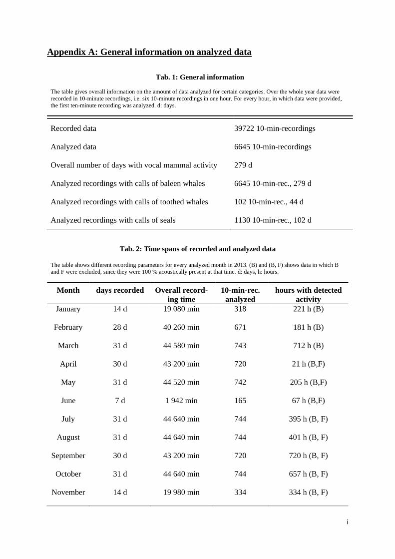
i
Appendix A: General information on analyzed data
Tab. 1: General information
The table gives overall information on the amount of data analyzed for certain categories. Over the whole year data were
recorded in 10-minute recordings, i.e. six 10-minute recordings in one hour. For every hour, in which data were provided,
the first ten-minute recording was analyzed. d: days.
Recorded data 39722 10-min-recordings
Analyzed data 6645 10-min-recordings
Overall number of days with vocal mammal activity 279 d
Analyzed recordings with calls of baleen whales 6645 10-min-rec., 279 d
Analyzed recordings with calls of toothed whales 102 10-min-rec., 44 d
Analyzed recordings with calls of seals 1130 10-min-rec., 102 d
Tab. 2: Time spans of recorded and analyzed data
The table shows different recording parameters for every analyzed month in 2013. (B) and (B, F) shows data in which B
and F were excluded, since they were 100 % acoustically present at that time. d: days, h: hours.
Month days recorded Overall record-
ing time
10-min-rec.
analyzed
hours with detected
activity
January 14 d 19 080 min 318 221 h (B)
February 28 d 40 260 min 671 181 h (B)
March 31 d 44 580 min 743 712 h (B)
April 30 d 43 200 min 720 21 h (B,F)
May 31 d 44 520 min 742 205 h (B,F)
June 7 d 1 942 min 165 67 h (B,F)
July 31 d 44 640 min 744 395 h (B, F)
August 31 d 44 640 min 744 401 h (B, F)
September 30 d 43 200 min 720 720 h (B, F)
October 31 d 44 640 min 744 657 h (B, F)
November 14 d 19 980 min 334 334 h (B, F)

Appendix B: Ice concentration
a)
b)
c)
d)
e)
f)
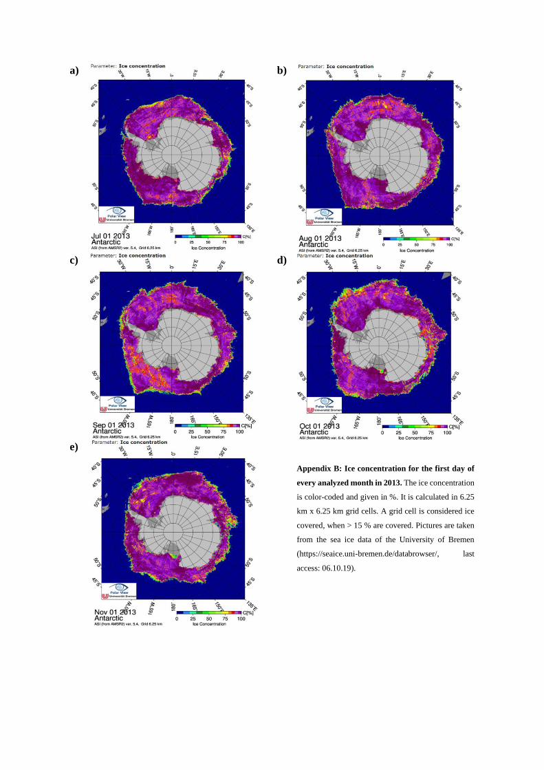
a)
b)
c)
d)
e)
Appendix B: Ice concentration for the first day of
every analyzed month in 2013. The ice concentration
is color-coded and given in %. It is calculated in 6.25
km x 6.25 km grid cells. A grid cell is considered ice
covered, when > 15 % are covered. Pictures are taken
from the sea ice data of the University of Bremen
(https://seaice.uni-bremen.de/databrowser/, last
access: 06.10.19).
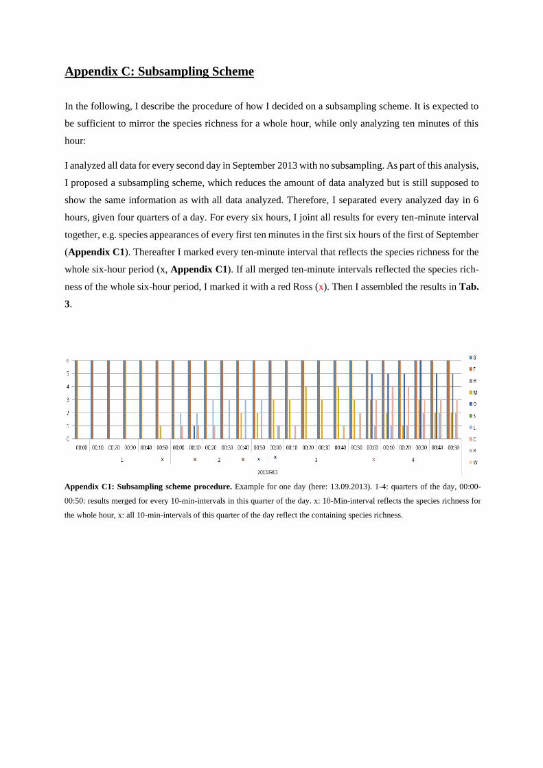
Appendix C: Subsampling Scheme
In the following, I describe the procedure of how I decided on a subsampling scheme. It is expected to
be sufficient to mirror the species richness for a whole hour, while only analyzing ten minutes of this
hour:
I analyzed all data for every second day in September 2013 with no subsampling. As part of this analysis,
I proposed a subsampling scheme, which reduces the amount of data analyzed but is still supposed to
show the same information as with all data analyzed. Therefore, I separated every analyzed day in 6
hours, given four quarters of a day. For every six hours, I joint all results for every ten-minute interval
together, e.g. species appearances of every first ten minutes in the first six hours of the first of September
(Appendix C1). Thereafter I marked every ten-minute interval that reflects the species richness for the
whole six-hour period (x, Appendix C1). If all merged ten-minute intervals reflected the species rich-
ness of the whole six-hour period, I marked it with a red Ross (x). Then I assembled the results in Tab.
3.
Appendix C1: Subsampling scheme procedure. Example for one day (here: 13.09.2013). 1-4: quarters of the day, 00:00-
00:50: results merged for every 10-min-intervals in this quarter of the day. x: 10-Min-interval reflects the species richness for
the whole hour, x: all 10-min-intervals of this quarter of the day reflect the containing species richness.

Tab. 3: Results for subsampling scheme procedure.
All results are assembled in one table to get an overall view and Find out the most fitting 10-min-interval to describe the
species richness for the whole hour. In case of my former study the first ten minutes showed the best results to mirror the
species richness of the whole following hour (see “Sum” in table).

Appendix D: Tables to different vocal activities
Tab. 4: Vocal activity of baleen whale species
Baleen whale species Time of detected vocal activity
Blue whales 279 d, 6645 h
Fin whales 250 d, 5754 h
Humpback whales 25 d, 108 h
Minke whales 156 d, 2188 h
Tab. 5: Vocal activity of toothed whale species
Toothed whale species Time of detected vocal activity
Killer whales 42 d, 95 h
Sperm whales 3 d, 11 h
Tab. 6: Vocal activity of seal species
Seal species Time of detected vocal activity
Leopard seals 32 d, 178 h
Crabeater seals 91 d, 1147 h
Ross seals 10 d, 77 h
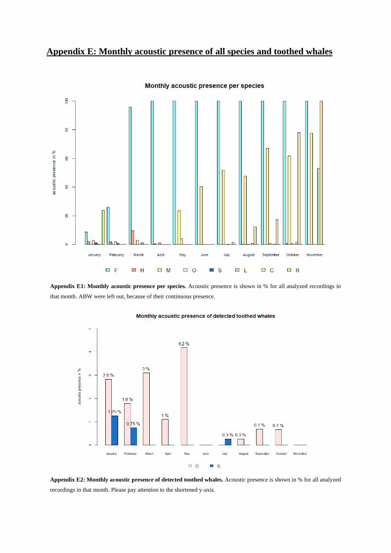
Appendix E: Monthly acoustic presence of all species and toothed whales
Appendix E2: Monthly acoustic presence of detected toothed whales. Acoustic presence is shown in % for all analyzed
recordings in that month. Please pay attention to the shortened y-axis.
Appendix E1: Monthly acoustic presence per species. Acoustic presence is shown in % for all analyzed recordings in
that month. ABW were left out, because of their continuous presence.
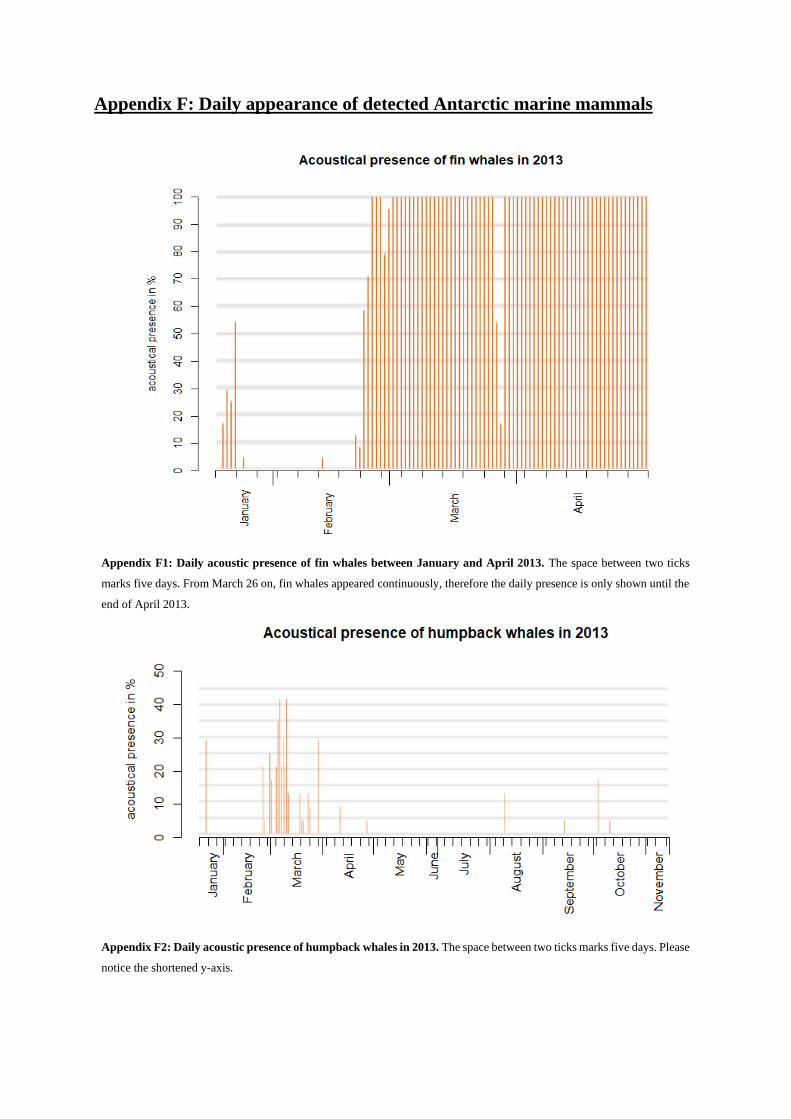
Appendix F: Daily appearance of detected Antarctic marine mammals
Appendix F1: Daily acoustic presence of fin whales between January and April 2013. The space between two ticks
marks five days. From March 26 on, fin whales appeared continuously, therefore the daily presence is only shown until the
end of April 2013.
Appendix F2: Daily acoustic presence of humpback whales in 2013. The space between two ticks marks five days. Please
notice the shortened y-axis.
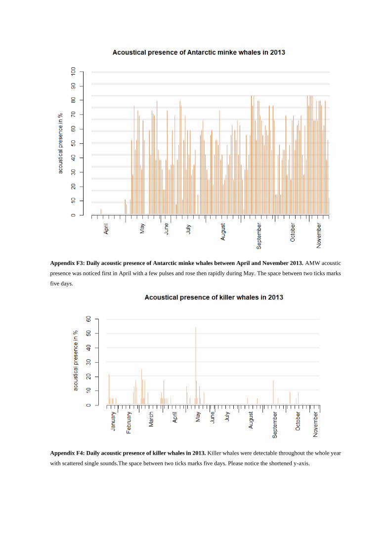
Appendix F3: Daily acoustic presence of Antarctic minke whales between April and November 2013. AMW acoustic
presence was noticed first in April with a few pulses and rose then rapidly during May. The space between two ticks marks
five days.
Appendix F4: Daily acoustic presence of killer whales in 2013. Killer whales were detectable throughout the whole year
with scattered single sounds.The space between two ticks marks five days. Please notice the shortened y-axis.
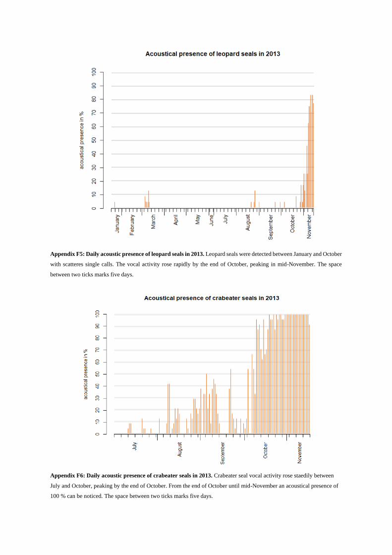
Appendix F5: Daily acoustic presence of leopard seals in 2013. Leopard seals were detected between January and October
with scatteres single calls. The vocal activity rose rapidly by the end of October, peaking in mid-November. The space
between two ticks marks five days.
Appendix F6: Daily acoustic presence of crabeater seals in 2013. Crabeater seal vocal activity rose staedily between
July and October, peaking by the end of October. From the end of October until mid-November an acoustical presence of
100 % can be noticed. The space between two ticks marks five days.
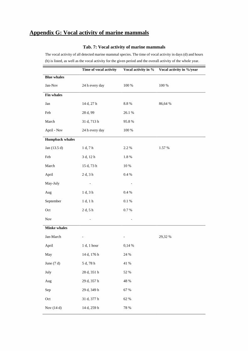
Appendix G: Vocal activity of marine mammals
Tab. 7: Vocal activity of marine mammals
The vocal activity of all detected marine mammal species. The time of vocal activity in days (d) and hours
(h) is listed, as well as the vocal activity for the given period and the overall activity of the whole year.
Time of vocal activity Vocal activity in % Vocal activity in %/year
Blue whales
Jan-Nov 24 h every day 100 % 100 %
Fin whales
Jan 14 d, 27 h 8.8 % 86,64 %
Feb 28 d, 99 26.1 %
March 31 d, 713 h 95.8 %
April - Nov 24 h every day 100 %
Humpback whales
Jan (13.5 d) 1 d, 7 h 2.2 % 1.57 %
Feb 3 d, 12 h 1.8 %
March 15 d, 73 h 10 %
April 2 d, 3 h 0.4 %
May-July - -
Aug 1 d, 3 h 0.4 %
September 1 d, 1 h 0.1 %
Oct 2 d, 5 h 0.7 %
Nov - -
Minke whales
Jan-March - - 29,32 %
April 1 d, 1 hour 0,14 %
May 14 d, 176 h 24 %
June (7 d) 5 d, 78 h 41 %
July 28 d, 351 h 52 %
Aug 29 d, 357 h 48 %
Sep 29 d, 349 h 67 %
Oct 31 d, 377 h 62 %
Nov (14 d) 14 d, 259 h 78 %
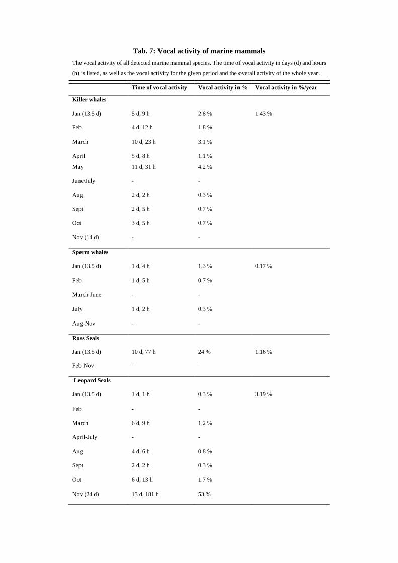
Tab. 7: Vocal activity of marine mammals
The vocal activity of all detected marine mammal species. The time of vocal activity in days (d) and hours
(h) is listed, as well as the vocal activity for the given period and the overall activity of the whole year.
Time of vocal activity Vocal activity in % Vocal activity in %/year
Killer whales
Jan (13.5 d) 5 d, 9 h 2.8 % 1.43 %
Feb 4 d, 12 h 1.8 %
March 10 d, 23 h 3.1 %
April 5 d, 8 h 1.1 %
May 11 d, 31 h 4.2 %
June/July - -
Aug 2 d, 2 h 0.3 %
Sept 2 d, 5 h 0.7 %
Oct 3 d, 5 h 0.7 %
Nov (14 d) - -
Sperm whales
Jan (13.5 d) 1 d, 4 h 1.3 % 0.17 %
Feb 1 d, 5 h 0.7 %
March-June - -
July 1 d, 2 h 0.3 %
Aug-Nov - -
Ross Seals
Jan (13.5 d) 10 d, 77 h 24 % 1.16 %
Feb-Nov - -
Leopard Seals
Jan (13.5 d) 1 d, 1 h 0.3 % 3.19 %
Feb - -
March 6 d, 9 h 1.2 %
April-July - -
Aug 4 d, 6 h 0.8 %
Sept 2 d, 2 h 0.3 %
Oct 6 d, 13 h 1.7 %
Nov (24 d) 13 d, 181 h 53 %
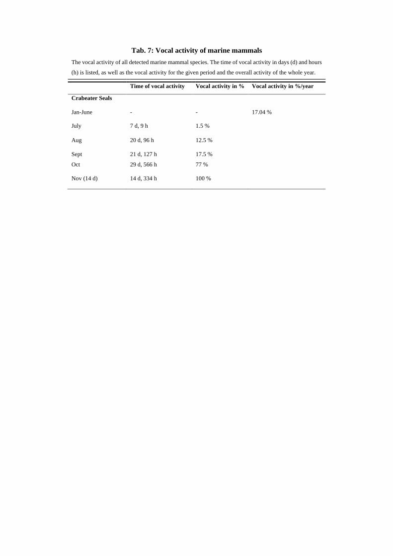
Tab. 7: Vocal activity of marine mammals
The vocal activity of all detected marine mammal species. The time of vocal activity in days (d) and hours
(h) is listed, as well as the vocal activity for the given period and the overall activity of the whole year.
Time of vocal activity Vocal activity in % Vocal activity in %/year
Crabeater Seals
Jan-June - - 17.04 %
July 7 d, 9 h 1.5 %
Aug 20 d, 96 h 12.5 %
Sept 21 d, 127 h 17.5 %
Oct 29 d, 566 h 77 %
Nov (14 d) 14 d, 334 h 100 %
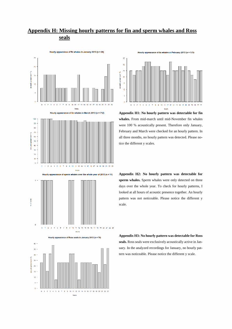
Appendix H: Missing hourly patterns for fin and sperm whales and Ross
seals
Appendix H1: No hourly pattern was detectable for fin
whales. From mid-march until mid-November fin whales
were 100 % acoustically present. Therefore only January,
February and March were checked for an hourly pattern. In
all three months, no hourly pattern was detected. Please no-
tice the different y scales.
Appendix H2: No hourly pattern was detectable for
sperm whales. Sperm whales were only detected on three
days over the whole year. To check for hourly patterns, I
looked at all hours of acoustic presence together. An hourly
pattern was not noticeable. Please notice the different y
scale.
Appendix H3: No hourly pattern was detectable for Ross
seals. Ross seals were exclusively acoustically active in Jan-
uary. In the analyzed recordings for January, no hourly pat-
tern was noticeable. Please notice the different y scale.
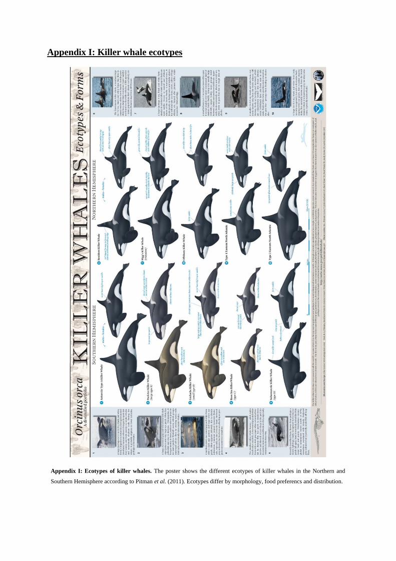
Appendix I: Killer whale ecotypes
Appendix I: Ecotypes of killer whales. The poster shows the different ecotypes of killer whales in the Northern and
Southern Hemisphere according to Pitman et al. (2011). Ecotypes differ by morphology, food preferencs and distribution.

Appendix J: Several killer and humpback whales vocalizing at the same
time
Appendix J1: Multiple killer whales. The spectrogram shows several pulsed clicks of killer whales. The temporally over
layering pulses presage multiple killer whales. The pulses were recorded May 6, 2013, at 11 pm. Hamming window, 90 %
overlap, DFT: 512 samples, ampl.: 20 times, FFT: 330 pts, fr: 7.6 Hz, tr: 0.13 s.
Appendix J2: Multiple humpback whales singing. During the song detected in my recordings, an echo was detected
several times, assuming that multiple male humpback whales are singing. The same structure of sound but with a lower
amplitude could indicate more distant males of the same population. It is also possible that the sound got reflected by
surfaces of, i.e. ice. The pulses were recorded March 10, 2013, at 10 pm. Hamming window, 90 % overlap, DFT: 512
samples, ampl.: 20 times, FFT: 420 pts, fr: 6 Hz, tr: 0.17 s

Acknowledgements
I would like to thank Dr. Ilse van Opzeeland for the chance to do a master thesis under her supervision.
Up until now that I finished my master thesis, I love my topic and am fascinated by everything I read
about marine mammals, the Southern Ocean and the ways and methods to get to know their habits.
Thank you for all the support, the answers to all my questions and for keeping me on my toes. It was
not always easy with me, but you taught me more than just distinguishing different marine mammal
vocalization and I am really grateful for that!
I would like to thank Dr. Irene Torrecilla Rocca for all the help, constructive criticism and support,
especially when it came to programming in R and biodiversity indices.
I would like to thank Prof. Dr. Gabriele Gerlach for reviewing my master thesis, but also for her support
and most importantly for giving me the advice to contact Ilse in the first place.
Also, I would like to thank Diego Filun from the Alfred Wegener Institute to provide the daily ice con-
centration data for my mooring location.
I would like to thank Simon Trautwein for great company, great talks and all the cookies he fed me,
when days got longer! I would like to thank Robin Fetzer and Maria Emrich for all the lunch breaks! I
would most definitely like to thank my flatmates for spontaneous breaks, great talks, for sharing your
food with me and for bringing me coffee!
Last but definitely not least, I would like to thank my family. We have not seen each other a lot in the
last months, but all the support and love via messages and photos arrived!

Eidesstattliche Erklärung
Hiermit versichere ich an Eides statt, dass ich diese Arbeit selbstständig verfasst und keine anderen als
die angegebenen Quellen und Hilfsmittel benutzt habe. Außerdem versichere ich, dass ich die allgemei-
nen Prinzipien wissenschaftlicher Arbeit und Veröffentlichung, wie sie in den Leitlinien guter wissen-
schaftlicher Praxis der Carl von Ossietzky Universität Oldenburg festgelegt sind, befolgt habe.
Unterschrift des Verfassers: ___________________________________________________________

© Paul Nicklen