AB HELSINKI UNIVERSITY OF TECHNOLOGY

Faculty of Electronics, Communications and Automation

Department of Communications and Networking

Timo-Pekka Heikkinen

Testing the Performance of a Commercial Active Network Measurement Platform

Thesis submitted in partial fulfillment of the requirements for the degree of Master of Science in Engineering Espoo, 31 March 2008 Supervisor: Professor Raimo Kantola Instructor: Lic. Sc. (Tech.) Marko Luoma

II

HELSINKI UNIVERSITY ABSTRACT OF THE OF TECHNOLOGY MASTER’S THESIS Author: Title: Date:

Timo-Pekka Heikkinen Testing the performance of a commercial active network measurement platform 31 March 2008 Language: English Number of pages: xi+80

Faculty: Department:

Faculty of Electronics, Communications and Automation Department of Communications and Networking Code: S-38

Supervisor: Instructor:

Professor Raimo Kantola Lic. Sc. (Tech.) Marko Luoma

In this thesis, a commercial active network measurement platform is tested for

performance and accuracy. The platform is also tested for ability to detect certain events

in networks. Two types of measurement probes are tested: the low performance Brix 100

Verifier and the high performance Brix 1000 Verifier. It is found that both platform’s

measurement probe types are accurate when measuring round-trip delay, but do not

perform nearly as well when measuring one-way delay. External synchronization, such as

GPS, helps the Brix 1000 Verifier to reach sub-millisecond measurement accuracy. As

Brix 100 Verifiers do not support external synchronization, their accuracy is suitable only

for measuring one-way delays larger than a few milliseconds.

The platform is able to detect sudden high load levels and router failures in a network, but

fails to detect short (sub-second) link breaks.

In the theory part of this thesis, some well known active measurement methods and

mechanisms are presented. Also, challenges related to active measurement are discussed

and some of the recent major academic active measurement projects are introduced.

Keywords: active measurement, network, packet loss, delay, available bandwidth, Brix, Verifier

III

TEKNILLINEN DIPLOMITYÖN KORKEAKOULU TIIVISTELMÄ Tekijä: Työn nimi: Päivämäärä:

Timo-Pekka Heikkinen Testing the performance of a commercial active network measurement platform 31.3.2008 Kieli: Englanti Sivumäärä: xi+80

Tiedekunta: Laitos:

Elektroniikan, tietoliikenteen ja automaation tiedekunta Tietoliikenne- ja tietoverkkotekniikan laitos Koodi: S-38

Valvoja: Ohjaaja:

Prof. Raimo Kantola TkL Marko Luoma

Diplomityössä testataan ja mitataan yhden kaupallisen aktiivimittausalustan suorituskyky

ja tarkkuus. Myös alustan kyky havaita tiettyjä tapahtumia tietoverkoissa testataan.

Testeissä on mukana kaksi erityyppistä alustaan kuuluvaa mittalaitetta: alhaisen

suorituskyvyn Brix 100 Verifier ja tehokkaampi Brix 1000 Verifier. Testauksen tuloksena

voidaan sanoa, että molemmat mittalaitetyypit soveltuvat hyvin kiertoaikaviiveen

mittaamiseen. Yhdensuuntaisen viiveen mittaukseen Brix 100 ei sovellu etenkään

mitattaessa alhaisia viivetasoja (~1ms). Ulkoista synkronisointilähdettä, kuten GPS-

kelloa, käytettäessä Brix 1000 –mittalaitetta voidaan käyttää myös yhdensuuntaisen

viiveen mittaamiseen.

Mittausalusta havaitsee verkossa tapahtuvat kuormitustilanteet ja reititinviat, mutta se ei

kykene havaitsemaan lyhyitä alle sekunnin mittaisia katkoja.

Työn teoriaosassa esitellään joitain tunnettuja aktiivimittausmekasimeja ja –metodeja

sekä pureudutaan aktiivimittauksiin ja niiden ongelmakohtiin yleisellä tasolla. Lisäksi

työssä esitellään tunnettuja akateemisia aktiivimittaukseen liittyviä projekteja.

Avainsanat: aktiivimittaukset, tietoverkko, pakettihukka, viive, vapaa kaistanleveys, Brix, Verifier

IV

Preface I would like to thank Professor Raimo Kantola, Lic. Sc. (Tech.) Marko Luoma and my other fellow workers. Special thanks to my wife Sanna and my co-workers Markus Peuhkuri, Juha Järvinen, Eero Solarmo, Olli-Pekka Lamminen and Oskari Simola. 31 March 2008, Espoo, Finland Timo-Pekka Heikkinen

V

Table of contents PREFACE..................................................................................................................................................... IV

TABLE OF CONTENTS...............................................................................................................................V

ACRONYMS ............................................................................................................................................. VIII

INDEX OF FIGURES....................................................................................................................................X

INDEX OF TABLES.................................................................................................................................... XI

1 INTRODUCTION........................................................................................................................................1

1.1 MOTIVATION ...................................................................................................................................1

2 BASIC TERMS AND NOTIONS................................................................................................................3

2.1.1 Path ...........................................................................................................................................3 2.1.2 Link capacity .............................................................................................................................3 2.1.3 Delay (latency) ..........................................................................................................................3 2.1.4 Packet delay variation and inter-arrival time variation (jitter) ................................................4 2.1.5 Queuing .....................................................................................................................................5 2.1.6 Packet loss, loss period and loss distance .................................................................................5 2.1.7 Throughput ................................................................................................................................6 2.1.8 Available Bandwidth .................................................................................................................6 2.1.9 Bulk Transfer Capacity..............................................................................................................7 2.1.10 Goodput ................................................................................................................................7 2.1.11 Probes...................................................................................................................................7 2.1.12 Metrics..................................................................................................................................8 2.1.13 Intrusiveness .........................................................................................................................8

2.2 ACTIVE VS. PASSIVE MEASUREMENTS.............................................................................................9 2.2.1 Passive measurements ...............................................................................................................9 2.2.2 Active measurements (probing) ...............................................................................................10 2.2.3 Hybrid measurements..............................................................................................................12

3 ACTIVE MEASUREMENTS ..................................................................................................................13

3.1 ACADEMIC RESEARCH PROJECTS FOCUSING ON ACTIVE MEASUREMENT .......................................13 3.2 NIMI.............................................................................................................................................13

3.2.1 Results and future work ...........................................................................................................15 3.2.2 References and publications....................................................................................................15

3.3 SURVEYOR....................................................................................................................................15 3.3.1 Results and future work ...........................................................................................................17 3.3.2 References and publications....................................................................................................17

3.4 IEPM PINGER ..............................................................................................................................18 3.4.1 Results and future work ...........................................................................................................19 3.4.2 References and publications....................................................................................................19

3.5 NLANR AMP...............................................................................................................................19 3.5.1 Results and future work ...........................................................................................................20 3.5.2 References and publications....................................................................................................20

3.6 SATURNE ......................................................................................................................................20 3.6.1 Results and future work ...........................................................................................................21 3.6.2 References and publications....................................................................................................21

3.7 COMPARISON BETWEEN DIFFERENT PROJECTS..............................................................................21 3.8 COMMERCIAL PERFORMANCE MEASUREMENT PRODUCTS.............................................................22 3.9 ACTIVE APPLICATION PERFORMANCE MEASUREMENTS.................................................................22 3.10 DEVICE PERFORMANCE TESTING...................................................................................................22 3.11 ACTIVE PROBING IN NETWORK SECURITY......................................................................................22

VI

3.12 LAYER 2 MEASUREMENTS.............................................................................................................23 3.12.1 Ethernet OAM.....................................................................................................................23 3.12.2 UDLD .................................................................................................................................24 3.12.3 Link layer (physical) topology discovery............................................................................24

3.13 MEASUREMENTS ON LAYER 2+ TO LAYER 4 .................................................................................24 3.13.1 MPLS/LSP-Ping..................................................................................................................25 3.13.2 Juniper Real-time Performance Monitor (RPM) ................................................................25 3.13.3 Cisco Service Assurance Agent / IOS IP Service Level Agreements...................................26 3.13.4 Active network layer topology discovery ............................................................................26 3.13.5 Reachability / Ping .............................................................................................................27 3.13.6 Route discovery / Traceroute..............................................................................................27 3.13.7 Path MTU discovery ...........................................................................................................28 3.13.8 Available bandwidth measurement methods and tools .......................................................28 3.13.9 Bulk transfer capacity.........................................................................................................30 3.13.10 IPMP...................................................................................................................................30 3.13.11 OWAMP..............................................................................................................................30 3.13.12 TWAMP ..............................................................................................................................31

3.14 BFD-PROTOCOL............................................................................................................................33 3.14.1 Operating modes.................................................................................................................33 3.14.2 Applications for BFD..........................................................................................................33

3.15 IPPM SPATIAL COMPOSITION........................................................................................................34 3.15.1 Justification ........................................................................................................................35 3.15.2 Accuracy and sources of error............................................................................................35 3.15.3 Spatial decomposition.........................................................................................................35

4 ACTIVE MEASUREMENT CHALLENGES........................................................................................36

4.1 MEASUREMENT PROTOCOLS.........................................................................................................36 4.2 SAMPLING .....................................................................................................................................36 4.3 END-TO-END MEASUREMENTS ON IP LAYER .................................................................................37 4.4 MEASURING PACKET LOSS............................................................................................................38 4.5 MEASURING AVAILABLE BANDWIDTH ...........................................................................................39 4.6 MEASURING DELAY ......................................................................................................................40

4.6.1 Timestamping and synchronization .........................................................................................41 4.6.2 GPS..........................................................................................................................................41 4.6.3 CDMA......................................................................................................................................42 4.6.4 NTP..........................................................................................................................................42 4.6.5 Accuracy of delay measurements ............................................................................................42 4.6.6 Error and uncertainty caused by clocks ..................................................................................43 4.6.7 One-way delay (OWD) ............................................................................................................44 4.6.8 Round-trip time (RTT) .............................................................................................................44

5 MEASUREMENT ARCHITECTURE AND DEVICES ............ ...........................................................45

5.1 BRIX NETWORKS’ MEASUREMENT PLATFORM .............................................................................45 5.1.1 Brix Verifiers ...........................................................................................................................46 5.1.2 BrixWorx software...................................................................................................................47 5.1.3 Configuring Brix Verifiers.......................................................................................................48 5.1.4 Bench configuring ...................................................................................................................48 5.1.5 Bench configuring Brix 100.....................................................................................................48 5.1.6 Bench configuring Brix 1000...................................................................................................49

5.2 ECHO-1 .........................................................................................................................................49 5.3 JUNIPER M7I .................................................................................................................................49 5.4 SPIRENT AX4000 (ADTECH) .........................................................................................................49

6 DELAY MEASUREMENT ACCURACY / PERFORMANCE TEST... ..............................................50

6.1 TEST SETUP...................................................................................................................................50 6.1.1 Traffic pattern..........................................................................................................................52

VII

6.1.2 Bandwidth usage .....................................................................................................................52 6.2 TEST RESULTS...............................................................................................................................53

6.2.1 Measured delay distribution....................................................................................................53 6.2.2 AX4000 ....................................................................................................................................54 6.2.3 Brix 1000 vs. Brix 1000...........................................................................................................55 6.2.4 Brix 100 vs. Brix 100...............................................................................................................56 6.2.5 Brix 1000 vs. Brix 100.............................................................................................................57 6.2.6 Juniper Real-time Performance Monitor (RPM).....................................................................58 6.2.7 Brix 1000 vs. Echo1.................................................................................................................60 6.2.8 Brix 100 vs. Echo1...................................................................................................................61 6.2.9 Brix 100 vs. Brix 100 RTT delay test .......................................................................................61

7 MEASUREMENTS IN A LIVE NETWORK.........................................................................................63

7.1 TEST NETWORK SETUP..................................................................................................................63 7.1.1 Network topology ....................................................................................................................63 7.1.2 Synchronization.......................................................................................................................64

7.2 MEASUREMENT SETUP..................................................................................................................64 7.2.1 UDP Echo test setup................................................................................................................65 7.2.2 Test traffic pattern ...................................................................................................................65 7.2.3 Bandwidth usage .....................................................................................................................65 7.2.4 Background load .....................................................................................................................65

7.3 TEST CASES AND RESULTS.............................................................................................................65 7.3.1 Load test ..................................................................................................................................66 7.3.2 Short link break test.................................................................................................................67 7.3.3 Node failure.............................................................................................................................68

8 CONCLUSIONS, RESULTS AND DISCUSSION.................................................................................70

8.1 PERFORMANCE TEST.....................................................................................................................70 8.2 LIVE NETWORK TEST.....................................................................................................................71 8.3 FUTURE WORK..............................................................................................................................72

9 REFERENCES..........................................................................................................................................73

VIII

Acronyms ACK Acknowledgement AMP Active Measurement Project API Application Programming Interface ATM Asynchronous Transfer Mode BFD Bidirectional Forwarding Detection BOOTP BOOTstrap Protocol Bps bits per second BSDI Berkeley Software Design Inc. BTC Bulk Transfer Capacity CAIDA Cooperative Association for Internet Data Analysis CC Continuity check CDMA Code Division Multiple Access CLI Command Line Interface CPOC Configuration Point of Contact DAC Data Analysis Client DB Database DHCP Dynamic Host Configuration Protocol DNS Domain Name System DSCP Differentiated Services Code Point DUT Device Under Test FEC Forwarding Equivalence Class FNAL Fermi National Accelerator Laboratory FTP File Transfer Protocol GPS Global Positioning System HMAC Hash Message Authentication Code HTTP Hyper Text Transfer Protocol ICMP Internet Control Message Protocol IEPM Internet End-to-end Performance Monitoring IETF Internet Engineering Task Force IGP Interior Gateway Protocol IP Internet Protocol IPFIX Internet Protocol Flow Information eXport IPMP IP Measurement Protocol IPPM IP Performance Metric ISP Internet Service Provider LAN Local Area Network LED Light Emitting Diode LSP Label Switched Path LSR Label Switching Router MC Measurement Client MIB Management Information Base MPLS Multiprotocol Label Switching MPOC Measurement Point of Contact MTU Maximum Transmission Unit NIMI National Internet Measurement Infastructure NLANR National Laboratory for Applied Network Research NMS Network Management System NTP Network Time Protocol OAM Operations, Administration and Maintenance OS Operating System OWAMP One Way Active Measurement Protocol OWD One-way Delay

IX

PASTA Poisson Arrivals See Time Averages PC Personal Computer PingER Ping End-to-end Reporting PMTU Path MTU PPS Pulse Per Second PPTD Packet Pair/Train Dispersion PVD Packet Delay Variation RED Random Early Detection RFC Request For Comments RIPE Réseaux IP Européens RMON Remote Network Monitoring RPC Remote Procedure Call RPM Real-time Performance Monitor RSA (Ron) Rivest (Adi) Shamir (and Leonard) Adleman, cryptographic

algorithm RTCP Real-Time Control Protocol RTP Real-time Transport Protocol RTT Round-trip Time SAA Service Assurance Agent SAMI Secure and Accountable Measurement Infrastructure SLA Service Level Agreement SLAC Stanford Linear Accelerator Center SLOPS Self-Loading Periodic Streams SNMP Simple Network Management Protocol SQL Structured Query Language TCP Transport Control Protocol TEIN Trans-Eurasia Information Network TOPP Trains of Packet Pairs ToS Type of Service TTL Time to Live TWAMP Two-way Active Measurement Protocol UDLD Unidirectional Link Detection UDP User Datagram Protocol UTC Universal Time, Coordinated VoIP Voice Over Internet Protocol VPN Virtual Private Network VPS Variable Packet Size VRF Virtual Routing and Forwarding VTHD Vraiment Très Haut Débit WAN Wide Area Network WWW World Wide Web XML Extensible Markup Language

X

Index of Figures FIGURE 1. DELAY TYPES. ....................................................................................................................................4 FIGURE 2. PACKET LOSS DISTANCE AND PERIOD...................................................................................................6 FIGURE 3. AN EXAMPLE OF A PASSIVE NETWORK MEASUREMENT. ........................................................................10 FIGURE 4. AN EXAMPLE OF ACTIVE NETWORK MEASUREMENT.............................................................................11 FIGURE 5. AN EXAMPLE OF A HYBRID MEASUREMENT. ........................................................................................12 FIGURE 6. NIMI ARCHITECTURE........................................................................................................................15 FIGURE 7. SURVEYOR MEASUREMENT ARCHITECTURE.........................................................................................17 FIGURE 8. PINGER INFRASTRUCTURE. ...............................................................................................................18 FIGURE 9. AN EXAMPLE OF A SIMPLE OWAMP TEST SETUP WHERE SEVERAL ROLES ARE PLAYED BY ONE END HOST.

...............................................................................................................................................................31 FIGURE 10. A SIMPLE EXAMPLE OF A TWAMP TEST SETUP WHERE MULTIPLE ROLES ARE PLAYED BY ONE ENTITY. 32 FIGURE 11. SPATIAL COMPOSITION....................................................................................................................34 FIGURE 12. MEASURING THE ONE-WAY DELAY OF A VOIP CALL IS PROBLEMATIC WHEN AN END-TO-END IP-LAYER

CONNECTION IS BROKEN INTO PARTS BY ONE OR MORE IP-IP-GATEWAYS....................................................37 FIGURE 13. AN EXAMPLE OF A DELAY DISTRIBUTION...........................................................................................39 FIGURE 14. NTP SERVER HIERARCHY.................................................................................................................42 FIGURE 15. BRIX MEASUREMENT PLATFORM. ....................................................................................................45 FIGURE 16. BRIX 100 VERIFIER’S REAR PANEL...................................................................................................46 FIGURE 17. CONNECTING A BRIX 100 VERIFIER. ................................................................................................47 FIGURE 18. PERFORMANCE TEST DEVICE AND CONNECTION SETUP.....................................................................51 FIGURE 19. TRAFFIC PATTERN...........................................................................................................................52 FIGURE 20. DIFFERENT TESTS CASES BETWEEN DEVICES.....................................................................................53 FIGURE 21. CUMULATIVE PROBABILITY DISTRIBUTION OF ONE-WAY DELAYS IN BRIX1000-BRIX1000, BRIX100-

BRIX100 AND AX4000-AX4000 TESTS. RESULTS SHOWN WITH AND WITHOUT NTP CORRECTION................54 FIGURE 22. ONE-WAY DELAY DISTRIBUTION (LEFT) AND BASELINE ONE-WAY DELAY (RIGHT) ................................55 FIGURE 23. THE FIGURE ON THE LEFT SHOWS ONE-WAY DELAY AFTER NTP STABILIZATION. THE FIGURE ON THE

RIGHT SHOWS HOW NTP STABILIZES AFTER A TIME DURING THE SYNCHRONIZATION PHASE.........................55 FIGURE 24. UNCORRECTED AND NTP-CORRECTED ONE-WAY DELAY AND DELAY DISTRIBUTIONS BETWEEN BRIX

1000 VERIFIERS. ......................................................................................................................................56 FIGURE 25. CORRECTED ONE-WAY DELAY BETWEEN BRIX 100 VERIFIERS............................................................57 FIGURE 26. UNCORRECTED AND CORRECTED ONE-WAY DELAY FROM BRIX1000-100 TEST. .................................58 FIGURE 27. MEASURED CLOCK OFFSET FROM A JUNIPER ROUTER DURING A TEST. ..............................................59 FIGURE 28. ROUND-TRIP DELAYS FROM JUNIPER EGRESS AND INGRESS ROUTERS. ...............................................59 FIGURE 29. ROUND-TRIP DELAY BETWEEN BRIX1000_1 AND ECHO1_1..............................................................60 FIGURE 30. ROUND-TRIP DELAY BETWEEN BRIX100_1 AND ECHO1_2................................................................61 FIGURE 31. AVERAGE RTT DISTRIBUTION BETWEEN TWO BRIX 100 VERIFIERS.....................................................62 FIGURE 32. NETWORK TOPOLOGY AND MEASUREMENT DEVICE PLACEMENT........................................................64 FIGURE 33. NTP-SETUP IN THE TEST NETWORK. ................................................................................................64 FIGURE 34. EFFECTS OF HIGH LOAD ON THE DELAY MEASURED BY THE BRIX SYSTEM. .........................................66 FIGURE 35. MEASURED PACKET LOSS FROM THE SHORT LINK BREAK TEST. .........................................................67 FIGURE 36. ROUTER FAILURE TEST. BRIX 2’S EDGE ROUTER FAILS. ....................................................................68

XI

Index of Tables TABLE 1. TERMS AND NOTIONS RELATING TO AVAILABLE BANDWIDTH MEASUREMENT............................................7 TABLE 2. COMPARISON BETWEEN ACTIVE MEASUREMENT PROJECTS...................................................................21 TABLE 3. TEST PARAMETER VALUES...................................................................................................................51 TABLE 4. MINIMUM AND MAXIMUM ONE-WAY DELAY RESULTS FROM THE PERFORMANCE TEST. ...........................54 TABLE 5. UDP ECHO TEST PARAMETER VALUES................................................................................................65 TABLE 6. BACKGROUND LOAD LEVELS DURING LOAD TEST.................................................................................66

1

Chapter 1

Introduction While delay or packet loss can be measured with either passive or active means, in this thesis the focus is on active measurements. Hence if it is not otherwise specifically mentioned all measurement methods and discussion concerns the active measurement viewpoint. Goals of this thesis are to introduce the reader to active measurements in data networks, benchmark one commercially available active measurement platform and analyze the measurement results gathered by using the aforementioned measurement system. The thesis is divided into three parts according to the goals: the theory part, benchmarking part and measurement part. In the first part the theory behind active network measurements is revealed and some basic concepts are presented. Some of the current and recent academic projects focusing on active measurements are listed and their results are discussed briefly. The focus of the first part is on discussing the notions of delay and packet loss that play an important part in the measurement and benchmarking chapters. The second part focuses on benchmarking a set of active measurement devices. This is done to find out how accurate and reliable their results are. The devices are compared against each other and one accurate industry-recognized measurement device which is used as a measurement standard. In the third part these devices are used to measure a live network. The results are analyzed and some conclusions are made of the devices and their applicability to measuring networks.

1.1 Motivation Why should networks be measured? For network operators it is important to know how well their network performs so that they know what kinds of services they are able to offer to their customers. A customer may want a virtual private network (VPN) connection that has a guaranteed level of delay, packet loss, availability etc. in which case a service level agreement (SLA) is negotiated between the customer and the service provider. The

2

operator has to know if it is able to provide such a service and this means that in addition to making some calculations based on the level of available resources in the operator’s network the performance of the network has to be tested in real life. The customer may want to actively test and measure the purchased service to see if the quality of the service is on the agreed level (SLA auditing). This requires active end-to-end network measurement since the customer does not own the network and thus he/she does not have access to the intermediate devices such as the provider’s core routers. In addition to measuring performance, network operators use active measurements to troubleshoot their network. In some cases there might be a fault in the network that causes traffic to be routed the wrong way. Generating an artificial traffic flow through the network and inspecting its behavior can help to troubleshoot routing faults. When introducing a new application or service to a network it is necessary to test the performance of the application before making it available for the users. Active measuring can be used to simulate a large number of users thus it can help in finding out for example how many simultaneous users a web server can service. Passive monitoring in conjunction with active probing (this is called hybrid measurement) can be used in finding out how a new service impacts the network both from the end-user’s and the network operator’s point of view.

3

Chapter 2

Basic terms and notions In this chapter some basic notions and terms related to computer networks are listed. These notions are explained in the sense they are used in this thesis.

2.1.1 Path A sequence of links from a source node S to destination node D is called a (network) path. Also the nodes connecting the links can be considered to be a part of the path.

2.1.2 Link capacity The capacity of a link is the maximum transfer rate possible for that link [1]. It must be noted that link capacity is defined per protocol layer. This means that the link capacity on Layer 2 is different from the link capacity on Layer 3 although the physical link is the same. The capacity C of an end-to-end path is the minimum link capacity iC in the path:

iCC min= , (1)

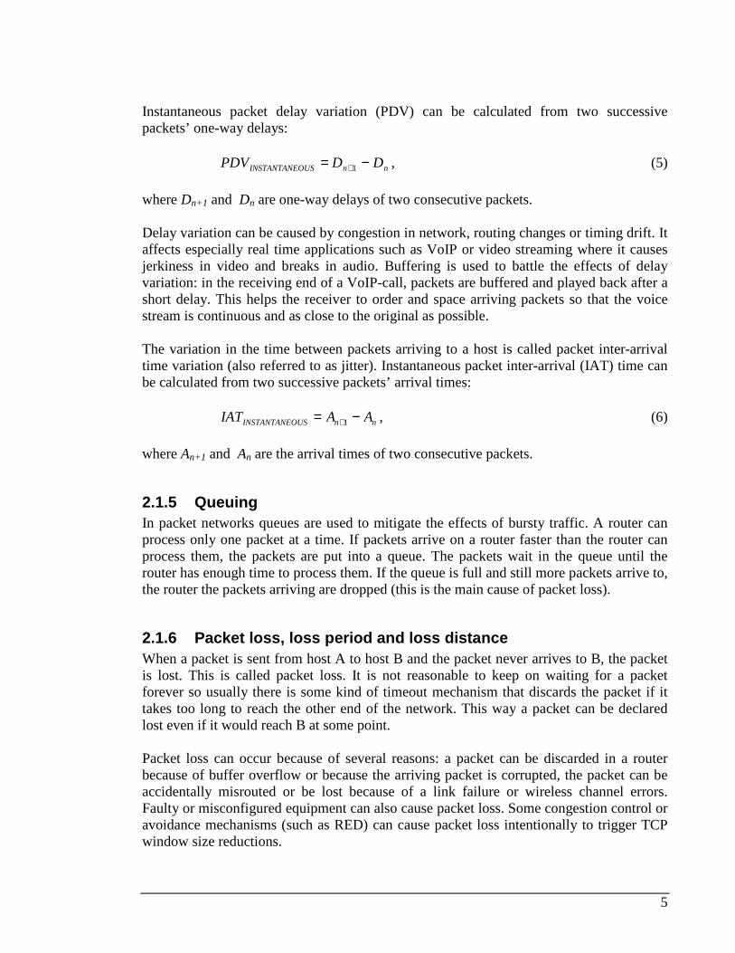
2.1.3 Delay (latency) In telecommunications there are several types of delay such as processing delay, propagation delay, queuing delay and transmission delay. In this thesis the notion of delay includes all the mentioned delay types and can be thus called end-to-end delay.

QUEUINGNPROPAGATIOONTRANSMISSIPROCESSING DDDDD +++=E2E (2)

Processing delay is the sum of delays caused by all the intermediate nodes on the network path processing the packet. A router needs to examine the arriving packet’s header to determine where to direct the packet. It also does bit-level error checking to see if the packet is corrupted and it may also process the packet by doing e.g. firewalling, encryption etc. All these functions the router performs add to the delay caused by processing. Processing delay mainly occurs on the edge routers of the network.

4

Transmission delay (or serialization delay) is the time it takes to send out a packet at the bit rate of the link. In other words transmission delay is the amount of time required by a router to push the entire packet onto the link.

R

LD ONTRANSMISSI = , (3)

where L is the length of the packet and R is the transmission rate of the link. Propagation delay is the time required for the signal to travel from one end of the transmission medium to the other. The delay depends on the physical medium and thus the delay is the distance between two end-points divided by the propagation speed.

c

dD NPROPAGATIO η

= , (4)

where d is the distance, c is the speed of light and η ≤ 1. Queuing delay is the amount of time a packet spends inside routers’ queues on its way from the source node to the destination node. Queuing delay is proportional to the buffer size and the amount of cross-traffic entering the router.

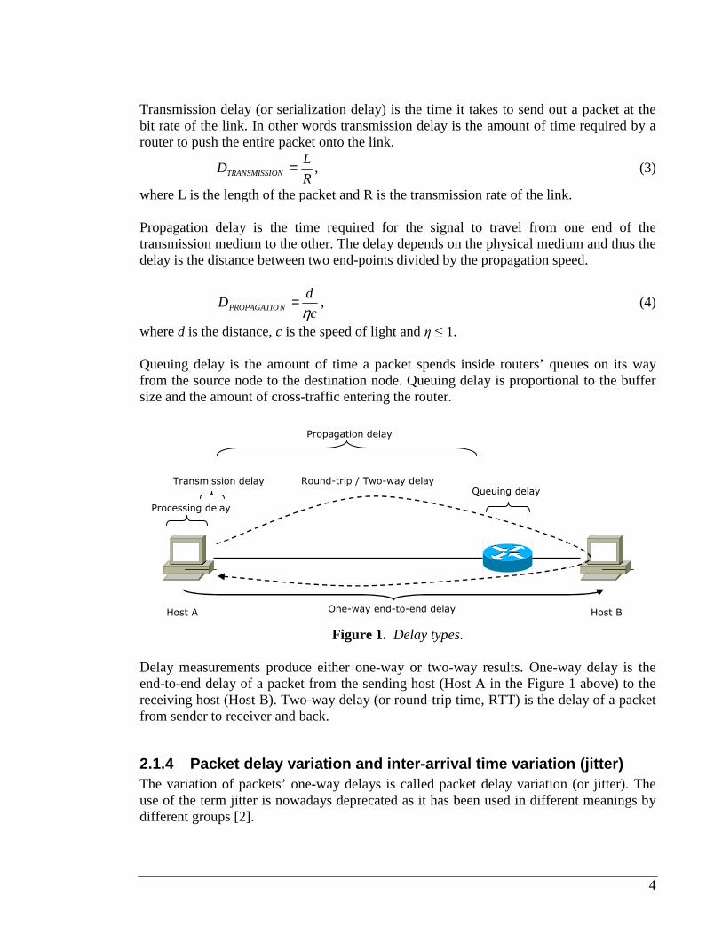
Figure 1. Delay types.

Delay measurements produce either one-way or two-way results. One-way delay is the end-to-end delay of a packet from the sending host (Host A in the Figure 1 above) to the receiving host (Host B). Two-way delay (or round-trip time, RTT) is the delay of a packet from sender to receiver and back.

2.1.4 Packet delay variation and inter-arrival time variation (jitter) The variation of packets’ one-way delays is called packet delay variation (or jitter). The use of the term jitter is nowadays deprecated as it has been used in different meanings by different groups [2].

Processing delay

Transmission delay

Propagation delay

Queuing delay

One-way end-to-end delay Host A Host B

Round-trip / Two-way delay

5

Instantaneous packet delay variation (PDV) can be calculated from two successive packets’ one-way delays:

nnOUSINSTANTANE DDPDV −= +1 , (5)

where Dn+1 and Dn are one-way delays of two consecutive packets. Delay variation can be caused by congestion in network, routing changes or timing drift. It affects especially real time applications such as VoIP or video streaming where it causes jerkiness in video and breaks in audio. Buffering is used to battle the effects of delay variation: in the receiving end of a VoIP-call, packets are buffered and played back after a short delay. This helps the receiver to order and space arriving packets so that the voice stream is continuous and as close to the original as possible. The variation in the time between packets arriving to a host is called packet inter-arrival time variation (also referred to as jitter). Instantaneous packet inter-arrival (IAT) time can be calculated from two successive packets’ arrival times:

nnOUSINSTANTANE AAIAT −= +1 , (6)

where An+1 and An are the arrival times of two consecutive packets.

2.1.5 Queuing In packet networks queues are used to mitigate the effects of bursty traffic. A router can process only one packet at a time. If packets arrive on a router faster than the router can process them, the packets are put into a queue. The packets wait in the queue until the router has enough time to process them. If the queue is full and still more packets arrive to, the router the packets arriving are dropped (this is the main cause of packet loss).

2.1.6 Packet loss, loss period and loss distance When a packet is sent from host A to host B and the packet never arrives to B, the packet is lost. This is called packet loss. It is not reasonable to keep on waiting for a packet forever so usually there is some kind of timeout mechanism that discards the packet if it takes too long to reach the other end of the network. This way a packet can be declared lost even if it would reach B at some point. Packet loss can occur because of several reasons: a packet can be discarded in a router because of buffer overflow or because the arriving packet is corrupted, the packet can be accidentally misrouted or be lost because of a link failure or wireless channel errors. Faulty or misconfigured equipment can also cause packet loss. Some congestion control or avoidance mechanisms (such as RED) can cause packet loss intentionally to trigger TCP window size reductions.

6

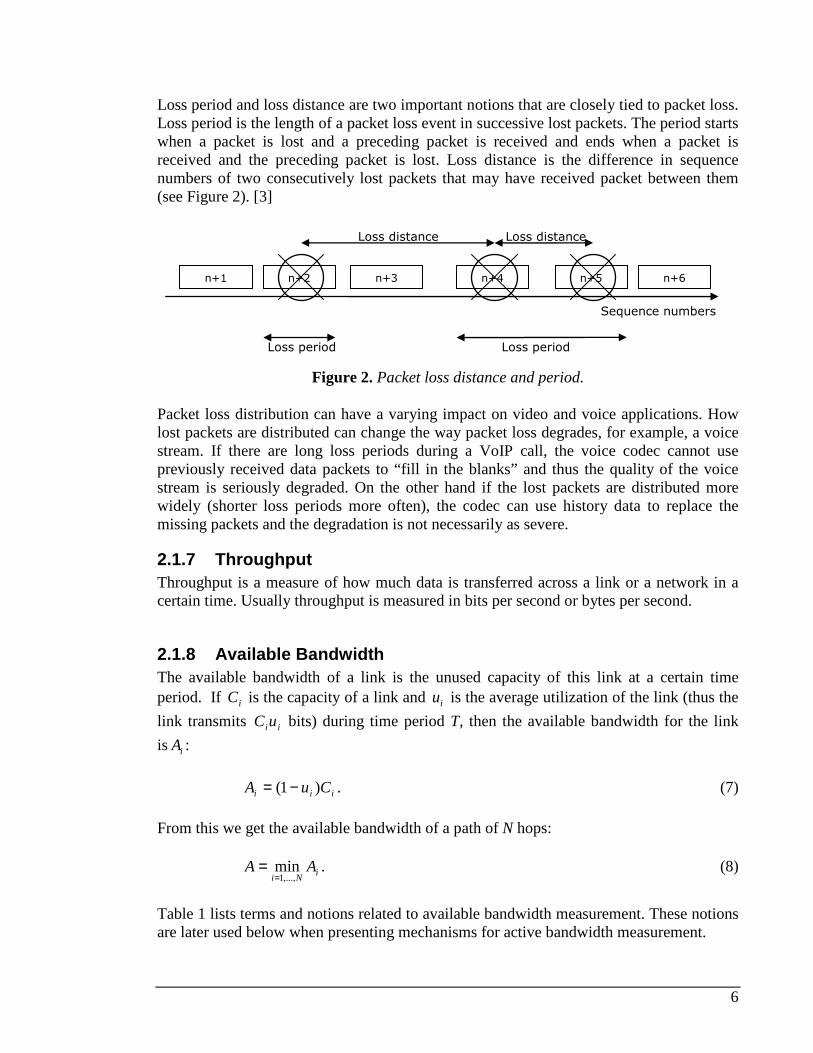
Loss period and loss distance are two important notions that are closely tied to packet loss. Loss period is the length of a packet loss event in successive lost packets. The period starts when a packet is lost and a preceding packet is received and ends when a packet is received and the preceding packet is lost. Loss distance is the difference in sequence numbers of two consecutively lost packets that may have received packet between them (see Figure 2). [3]

Figure 2. Packet loss distance and period.

Packet loss distribution can have a varying impact on video and voice applications. How lost packets are distributed can change the way packet loss degrades, for example, a voice stream. If there are long loss periods during a VoIP call, the voice codec cannot use previously received data packets to “fill in the blanks” and thus the quality of the voice stream is seriously degraded. On the other hand if the lost packets are distributed more widely (shorter loss periods more often), the codec can use history data to replace the missing packets and the degradation is not necessarily as severe.

2.1.7 Throughput Throughput is a measure of how much data is transferred across a link or a network in a certain time. Usually throughput is measured in bits per second or bytes per second.

2.1.8 Available Bandwidth The available bandwidth of a link is the unused capacity of this link at a certain time period. If iC is the capacity of a link and iu is the average utilization of the link (thus the

link transmits iiuC bits) during time period T, then the available bandwidth for the link

is iA :

iii CuA )1( −= . (7)

From this we get the available bandwidth of a path of N hops:

iNi

AA,...,1

min=

= . (8)

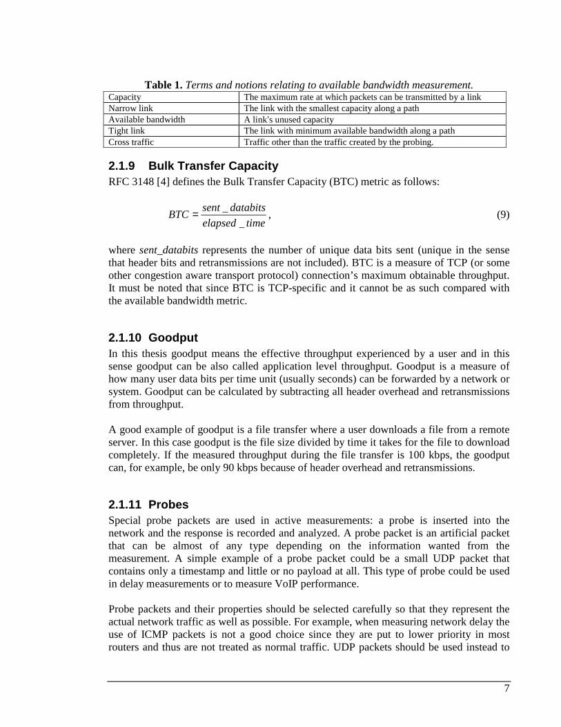
Table 1 lists terms and notions related to available bandwidth measurement. These notions are later used below when presenting mechanisms for active bandwidth measurement.

n+1 n+2 n+3 n+4 n+5 n+6

Loss period

Loss distance Loss distance

Loss period

Sequence numbers

7

Table 1. Terms and notions relating to available bandwidth measurement.

Capacity The maximum rate at which packets can be transmitted by a link Narrow link The link with the smallest capacity along a path Available bandwidth A link ’s unused capacity Tight link The link with minimum available bandwidth along a path Cross traffic Traffic other than the traffic created by the probing.

2.1.9 Bulk Transfer Capacity RFC 3148 [4] defines the Bulk Transfer Capacity (BTC) metric as follows:

timeelapsed

databitssentBTC

_

_= , (9)

where sent_databits represents the number of unique data bits sent (unique in the sense that header bits and retransmissions are not included). BTC is a measure of TCP (or some other congestion aware transport protocol) connection’s maximum obtainable throughput. It must be noted that since BTC is TCP-specific and it cannot be as such compared with the available bandwidth metric.

2.1.10 Goodput In this thesis goodput means the effective throughput experienced by a user and in this sense goodput can be also called application level throughput. Goodput is a measure of how many user data bits per time unit (usually seconds) can be forwarded by a network or system. Goodput can be calculated by subtracting all header overhead and retransmissions from throughput. A good example of goodput is a file transfer where a user downloads a file from a remote server. In this case goodput is the file size divided by time it takes for the file to download completely. If the measured throughput during the file transfer is 100 kbps, the goodput can, for example, be only 90 kbps because of header overhead and retransmissions.

2.1.11 Probes Special probe packets are used in active measurements: a probe is inserted into the network and the response is recorded and analyzed. A probe packet is an artificial packet that can be almost of any type depending on the information wanted from the measurement. A simple example of a probe packet could be a small UDP packet that contains only a timestamp and little or no payload at all. This type of probe could be used in delay measurements or to measure VoIP performance. Probe packets and their properties should be selected carefully so that they represent the actual network traffic as well as possible. For example, when measuring network delay the use of ICMP packets is not a good choice since they are put to lower priority in most routers and thus are not treated as normal traffic. UDP packets should be used instead to

8

get a more realistic view of the network delay. Also such things as packet size and sending rate can be issues.

2.1.12 Metrics A metric is a quantity related to the performance and reliability of the Internet. It can also be said to be a generic indicator of how the network performs. One single measurement result of a metric is called a singleton metric, a set of distinct measurement results (singletons) is called a sample metric and a statistic calculated over a sample metric is called a statistic metric. [5] For example, a single active UDP echo test run between two hosts produces a round-trip time result that is considered a singleton metric. The same test repeated for n times in a row produces a sample metric. The mean of all measured round-trip values in the previous sample metric can be defined as a statistic metric. . The IETF IP Performance Metrics (IPPM) working group has proposed several metrics and procedures for accurately measuring and documenting the metrics. The following metrics have been published in a series of RFCs:

• Connectivity (RFC 2678) • One-way Delay (RFC 2679) • One-way Packet Loss (RFC 2680) • Round-trip Delay (RFC 2681) • One-way Loss Pattern Sample (RFC 3357) • IP Packet Delay Variation (RFC 3393) • Packet Reordering Metrics (RFC 4737)

Other metrics such as bulk transport and link bandwidth capacity are being developed by the IPPM.

2.1.13 Intrusiveness Active network measurement creates an additional load on the measured network and thus uses some of the available bandwidth. Intrusiveness is the property of a measurement tool that describes how much of the available bandwidth the tool consumes. For example, a tool or mechanism that consumes 90% of the available bandwidth on a network path can be considered intrusive. A tool that generates small UDP-packets to measure RTT every now and then can hardly be said intrusive (assuming that the available bandwidth of the path is not exceptionally low). According to [6] an active measurement tool or technique can be considered intrusive if its average probing load on the network during a measurement is significant when compared to the available bandwidth in the path.

9

2.2 Active vs. passive measurements Active and passive measurements produce different kinds of information and the results do not necessarily correlate well [7]. A more complete picture of the health of a network can be gained by combining results from both active and passive measurements (hybrid measurements). Although the focus in this thesis is on active measurements, differences in active and passive measurements will also be discussed briefly. Passive measurements are best suited to situations where capture points can be freely selected. This is true in situations where the whole network is owned and operated by a single organization (e.g. corporate premises networks). This allows traffic to be captured from any point on the path from the sender to the receiver. In situations where it is not possible to select capture points freely, active measurements have to be used. This is often the case when measuring delay performance of a VPN which is carried over multiple ISPs. Active measurements can be made over a network path that has parts which are not controlled by the measurer. When it comes to accuracy of measurements, passive methods are often more accurate. For example packet loss can be measured very accurately by monitoring router buffers along the network path. Also, available bandwidth can be accurately measured by monitoring link usage on routers. Both above mentioned measurements are difficult to do accurately with active probing. The problems related to active probing are discussed in chapter 4.

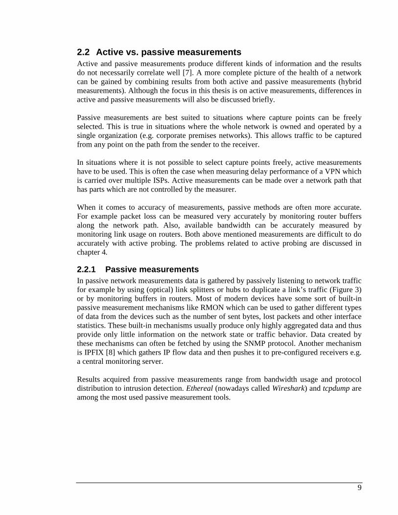
2.2.1 Passive measurements In passive network measurements data is gathered by passively listening to network traffic for example by using (optical) link splitters or hubs to duplicate a link’s traffic (Figure 3) or by monitoring buffers in routers. Most of modern devices have some sort of built-in passive measurement mechanisms like RMON which can be used to gather different types of data from the devices such as the number of sent bytes, lost packets and other interface statistics. These built-in mechanisms usually produce only highly aggregated data and thus provide only little information on the network state or traffic behavior. Data created by these mechanisms can often be fetched by using the SNMP protocol. Another mechanism is IPFIX [8] which gathers IP flow data and then pushes it to pre-configured receivers e.g. a central monitoring server. Results acquired from passive measurements range from bandwidth usage and protocol distribution to intrusion detection. Ethereal (nowadays called Wireshark) and tcpdump are among the most used passive measurement tools.

10

Figure 3. An example of a passive network measurement.

The main problem of passive measurements is the amount of data that is generated. If we assume a gigabit link with a utilization of 60% (on IP-layer) and an average packet size of 300 bytes, then the capture rate is about 250000 packets per second. The traffic rate is 75 mebibytes (MiBs) per second and thus the storage space needed for one hour trace is 270000 mebibytes (= 270 gibibytes). If there are several capture points in the network, the amount of captured data is going to be a problem. Depending on the type of measurement, several compression methods are available: all irrelevant data could be removed from the captured packets including the payload and some of the header fields. Normal compression methods can be used to remove redundancy from the packets (for example gzip can be used to further reduce the required storage space) [9]. Also, traffic sampling can be used when full traffic analysis is not required. Sampling can drastically reduce the amount of storage space needed but it has some drawbacks (difficulty of flow analysis [9]) and not all sampling methods produce good results [10]. Different sampling methods are discussed in [11]. If only the IP and transport layer headers were stored (40 bytes per packet), the example calculation above would yield a traffic rate of 10 megabytes per second and 36 gigabytes of storage space required for a one hour trace. The analysis of the captured data is also an issue; on-line analysis is difficult because of the large amount of data. If the capture is made from an operational network, there are privacy issues that need to be taken into account. This means that the captured traffic has to be modified in such a way that the IP-addresses are anonymized and the payload data has to be removed. A short discussion about the sensitivity of IP header fields and a method to anonymize packets is given in [12]. There are some advantages in passive measurements over active measurements. Passive methods do not create additional traffic thus they do not disturb the network and they provide an accurate representation of the network traffic.

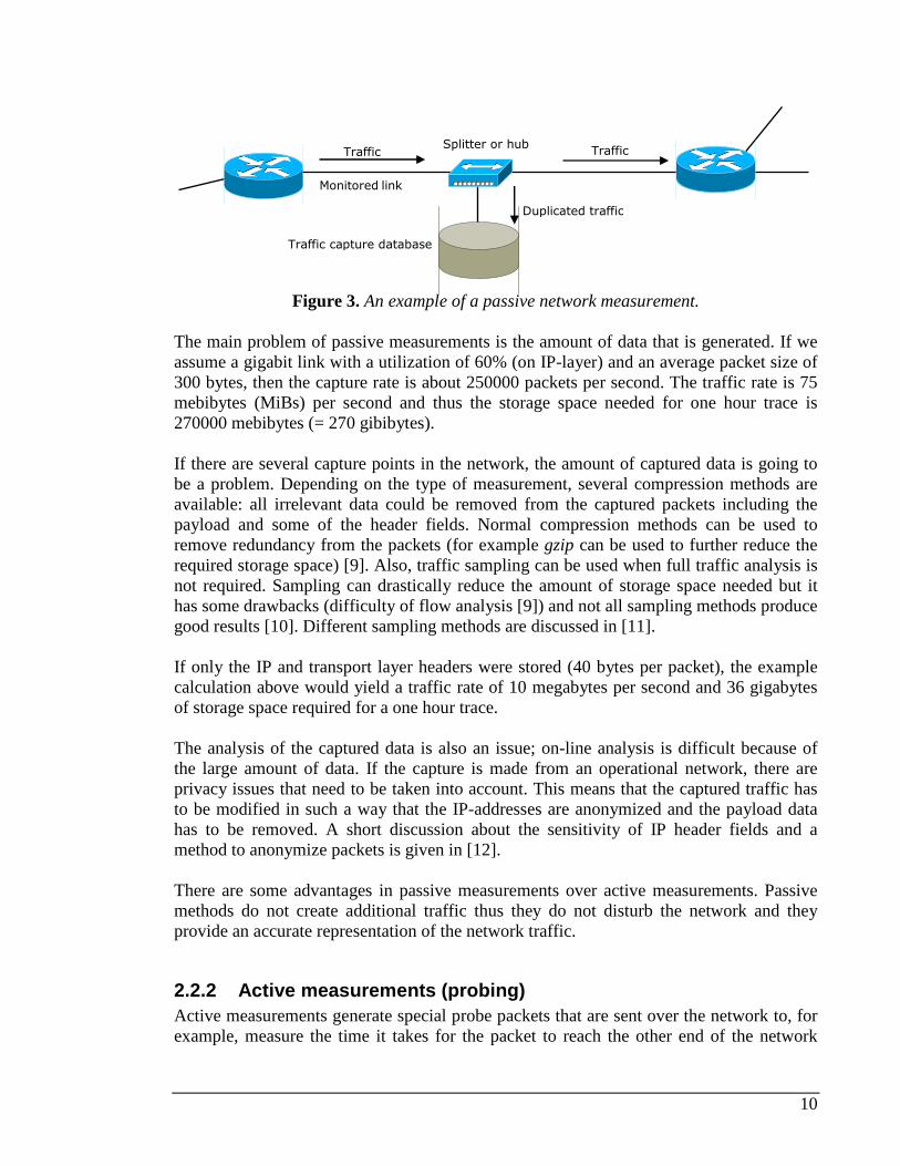
2.2.2 Active measurements (probing) Active measurements generate special probe packets that are sent over the network to, for example, measure the time it takes for the packet to reach the other end of the network

Monitored link

Traffic capture database

Splitter or hub Traffic

Duplicated traffic

Traffic

11

(one-way delay), the available capacity of a network path or the response time of an application. Unlike passive measurements, active measurements generate additional network traffic so they may possibly disturb the normal network traffic flow. This is why active measurements have to be carefully planned before execution and usually the bandwidth reserved for the probe packets is limited to fewer than 5 percent of the path’s total capacity. This is the case in most SLA-measurements where the measurement is done constantly meaning the test traffic and customer traffic share the same bandwidth. Some methods (e.g. SLOPS, see section 3.13.8) used for measuring the available bandwidth on a path consist in sending probe packets at an increasing rate and recording the rate at which the probe’s delays start to rise (meaning that packets are being queued at some point) [13]. These methods will cause perturbations in the normal traffic flow although the perturbations are usually short. Heisenberg’s (Werner Karl Heisenberg, December 5, 1901 – February 1, 1976, Germany) uncertainty principle can be interpreted to state that the act of measurement itself introduces (an irreducible) uncertainty to the measurements [14]. This is true in the case of active network measurements and especially in active packet-loss measurements, where the probe packets may cause congestion and therefore packet-loss. Passive measurement does not have this issue as no additional traffic is inserted into the measured system.

Figure 4. An example of active network measurement.

Active measurements do not require huge amounts of storage space and they can be used to measure things that are not possible by using passive measurements. Also, when using active probing, there are no privacy issues since the data used does not contain any private information. All active probe packets are artificial i.e. they are generated on demand and thus they usually contain only random bits as payload. The example presented in Figure 4 shows how active probing can be used to measure the response time of a web server. A measurement device or a software agent installed on a normal PC sends web page requests across a network and records the response time. The most well known active measurement tools are probably traceroute and ping which are built in to most operating systems. These two tools will be presented in more detail later.

Web server

Agent (web client)

Network

Generated traffic

Web page request

Web page response

12

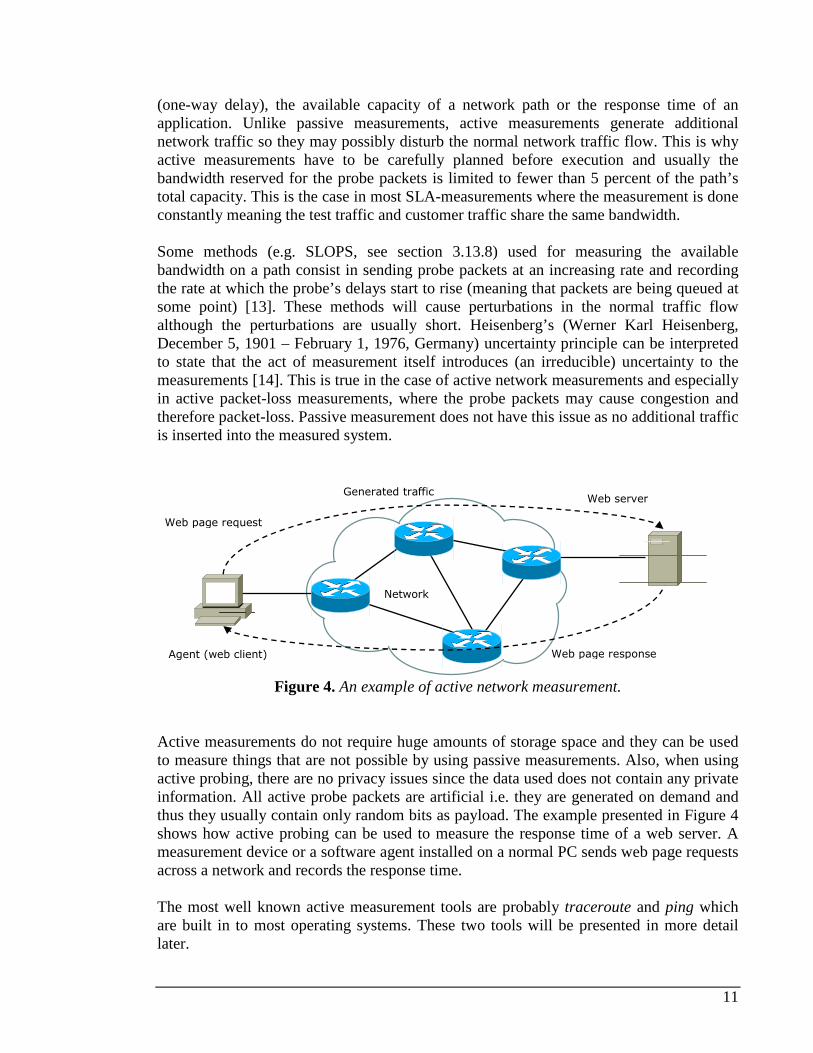
2.2.3 Hybrid measurements Combining active and passive measurements is called hybrid measurement. An example of a hybrid measurement (Figure 5) could be a scenario where active probes are sent over a network and their progress is monitored by passive means during the measurement. This type of arrangement allows the measurer to track the path of the probes and record the intermediate and end-to-end delays. This is something that is not possible by doing only active probing.

Figure 5. An example of a hybrid measurement.

The above scenario requires that the measurer has administrative access to the intermediate routers and is thus not suitable to Internet scale measurements. It must be noted that since hybrid measurements use both passive and active means, they share all the same issues as passive and active measurements.

Probe traffic

Passive monitoring / traffic capturing

13

Chapter 3 Active measurements In this chapter, some of the recent academic research projects focusing on active measurement are studied and their results are discussed briefly. In addition to research projects, this chapter lists known active measurement mechanisms, methodologies and tools. Also, different uses for active measurement are presented briefly.

3.1 Academic research projects focusing on active measurement

There are several research projects focusing on active measurement or measurement platforms in Internet environment. A selected group of these projects is briefly discussed below although most of these projects have already ended. This list is by no means comprehensive: there are many other projects out there such as RIPE [15].

3.2 NIMI National Internet Measurement Infrastructure (NIMI) is a measurement platform, or rather, a command and control system for managing measurement tools. NIMI aims at being a scalable large scale measurement platform. The ability to schedule measurements to take place in the future allows large scale measurements to be started simultaneously without the need to start every probe manually. With decentralized control of measurements and modular measurement tools NIMI looks like a promising tool for large scale network measurements. The NIMI architecture can be divided into two main areas: the structure of the individual platform and the different external components that control the platforms. A platform (also called a probe) performs different measurements using external tools such as traceroute, treno or zing and records the results. All data analyzing and visualization are done by external hosts. New measurement tools can be added to the platform as plug-in modules. This requires that a “wrapper” script is generated for the tool that helps the tool to fit the NIMI API. Each measurement platform includes a server, whose job is to handle such tasks as authenticating, queuing and executing measurement requests. The server also takes care of

14

bundling and shipping the results to a specified destination and deleting them after they are no longer needed. All messages sent between the NIMI components are, by default, encrypted and authenticated using RSA public and private key pairs. The software component of the NIMI probe is internally divided into two distinct components: nimid, and scheduled. The nimid daemon is responsible for communication with the outside world and performing access control checks. The scheduled daemon takes care of the measurement scheduling and result packaging. [16] The external components controlling the measurement platforms are listed and explained below:

• CPOC, Configuration Point of Contact • DAC, Data Analysis Client • MC, Measurement Client • MPOC, Measurement Point of Contact

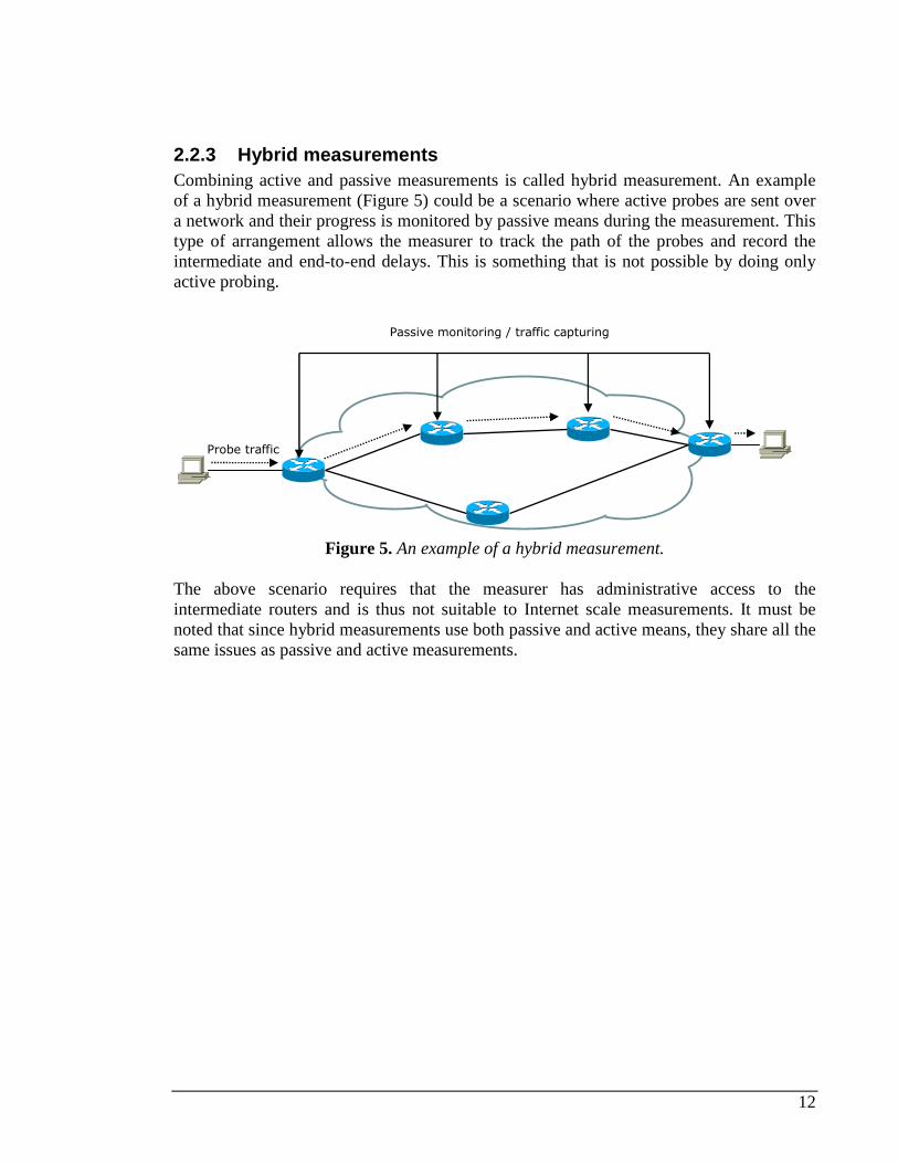
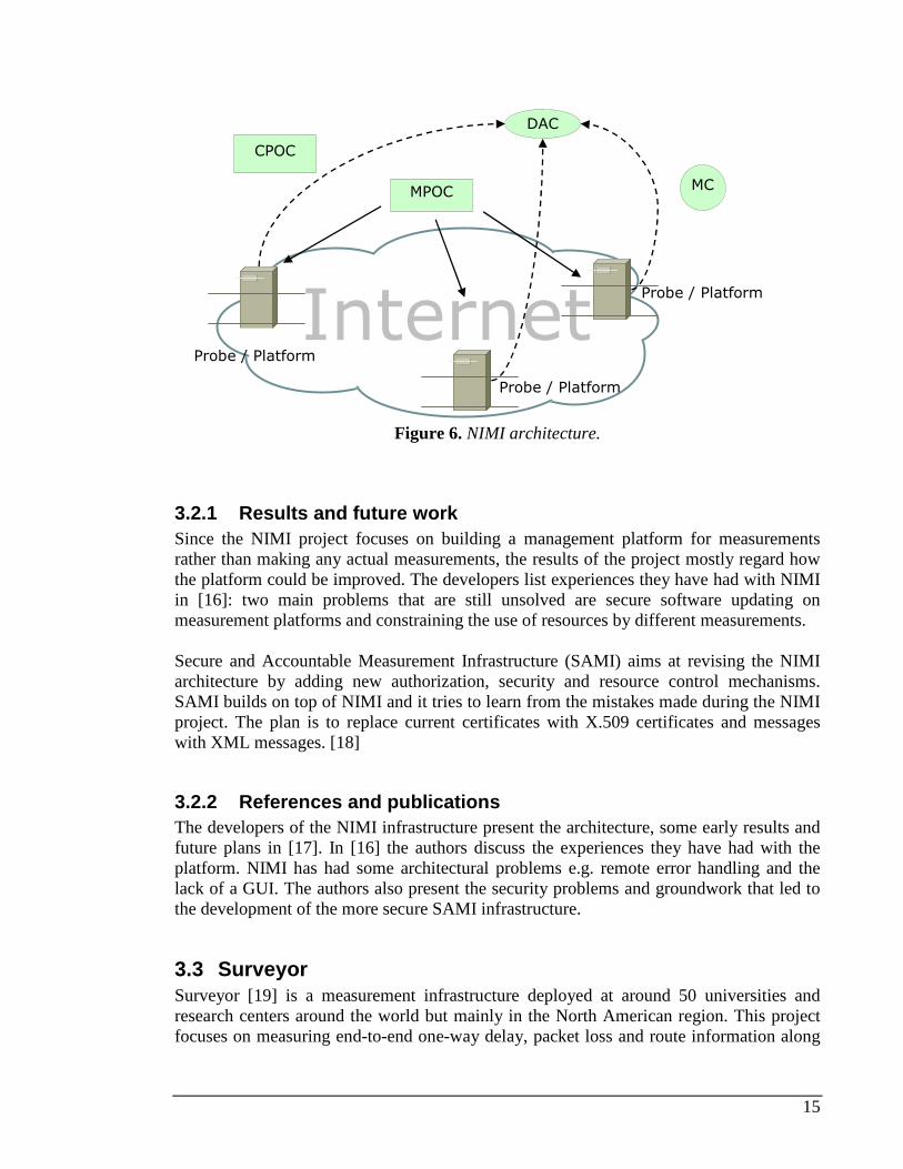
CPOC is the component that is used to configure and administer measurement platforms within the CPOC’s administrative domain. The CPOC provides each platform with its initial policies (access control lists etc.) and also updates these policies over time if needed. DAC is the component that is responsible for storing and post-processing the measurement data. After a probe completes a measurement, it sends its data out to a designated DAC. DAC can be run as a part of the MC, if the results are wanted immediately after the test or during the test. The measurement client (MC) is the only NIMI component that can be directly operated by the end user. It is a UNIX utility that can be run on any suitable host computer to directly communicate with the measurement probes. The MPOC component allows a set of measurements to be configured and prepared at a single location. The MPOC and CPOC functions are separated because it allows a site to delegate partial control of its NIMI daemons to an MPOC (or MPOCs) while still maintaining ultimate control locally. [17] Figure 6 displays the basic NIMI architecture. In the figure, CPOC is the component that gives the probes their initial configurations and MPOC the one that configures a test to be run on all three probes. After the test is finished, the probes send their measurement data to the DAC for analysis and (or) storage. The MC component can be used to control the probes and in some cases it can include the functionality of the MPOC, however this is not clear from the NIMI documents and the current NIMI implementations may differ from the one that is described in [16] and [17].

15

Figure 6. NIMI architecture.

3.2.1 Results and future work Since the NIMI project focuses on building a management platform for measurements rather than making any actual measurements, the results of the project mostly regard how the platform could be improved. The developers list experiences they have had with NIMI in [16]: two main problems that are still unsolved are secure software updating on measurement platforms and constraining the use of resources by different measurements. Secure and Accountable Measurement Infrastructure (SAMI) aims at revising the NIMI architecture by adding new authorization, security and resource control mechanisms. SAMI builds on top of NIMI and it tries to learn from the mistakes made during the NIMI project. The plan is to replace current certificates with X.509 certificates and messages with XML messages. [18]

3.2.2 References and publications The developers of the NIMI infrastructure present the architecture, some early results and future plans in [17]. In [16] the authors discuss the experiences they have had with the platform. NIMI has had some architectural problems e.g. remote error handling and the lack of a GUI. The authors also present the security problems and groundwork that led to the development of the more secure SAMI infrastructure.

3.3 Surveyor Surveyor [19] is a measurement infrastructure deployed at around 50 universities and research centers around the world but mainly in the North American region. This project focuses on measuring end-to-end one-way delay, packet loss and route information along

Internet

MPOC

CPOC

MC

DAC

Probe / Platform

Probe / Platform

Probe / Platform

16

Internet paths. The project ended around the year 2000 and it is now difficult to find information regarding Surveyor. Surveyor’s guiding principles to achieve measurement goals were:

• Use of standard metrics • Measurement of path’s one-way properties • Use of dedicated measurement devices • Continuous end-to-end measurements • Real-time access to long-term performance measurement data

The use of standard metrics (i.e. IPPM metrics) is required for the measurements to be comparable with other metrics and for general understanding of the measurement results. Since most of the Internet paths are asymmetrical in nature, it is better to measure one-way metrics than for example round-trip time. Due to maintenance, performance and security reasons the measurement machines are dedicated devices provided by the Surveyor organization. Continuous measurements are required to detect trends in the network behavior and to reduce the possibility of missing some events occurring in the network. The ability to provide real-time (or near real-time) long-term measurement data is important for network engineers performing troubleshooting or capacity planning. Surveyor archives all raw performance data this way aiding network researchers. To measure delay and packet loss Surveyor uses a Poisson process with λ=2 per second to send test packets. The average packet rate is thus two packets per second. Probe packets contain only a sequence number and a timestamp and their size is minimal of 12 bytes. Such properties for the probe packets were selected because of storage space and bandwidth limitations. Route information is gathered by using a modified version of traceroute. Changes made to the program are:

• 10 tries instead of the default 3 when a TTL exceeded ICMP message is not forthcoming

• No probes are sent after TTL success rather than sending all three probes in any case

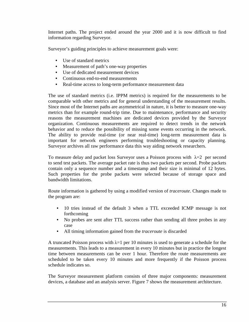
• All timing information gained from the traceroute is discarded A truncated Poisson process with λ=1 per 10 minutes is used to generate a schedule for the measurements. This leads to a measurement in every 10 minutes but in practice the longest time between measurements can be over 1 hour. Therefore the route measurements are scheduled to be taken every 10 minutes and more frequently if the Poisson process schedule indicates so. The Surveyor measurement platform consists of three major components: measurement devices, a database and an analysis server. Figure 7 shows the measurement architecture.

17

Figure 7. Surveyor measurement architecture.

Measurement devices are standard desktop PCs equipped with GPS receivers for accurate timing and appropriate type of interface card (Ethernet, ATM, FDDI). Each device runs measurement software on top of a modified BSDI operating system. Each measurement device buffers its measurement data on a local disk. Machines are polled for new measurement data every few minutes and the new data is transferred to the central database where all data is kept in binary files. Daily summary plots, traceroute data and some other statistics are made available using an HTTP server.

3.3.1 Results and future work The results from the Surveyor project mainly focus on the performance of the measured network. Two comparisons between Surveyor and other active measurement projects can be found online [20], [21]. In [22] the developers list lessons they have learned with Surveyor. The measurement infrastructure is able to detect Layer-2 changes in the network and it has proven that the measured high speed connections really provide low-latency and low-loss paths. They also note that the routing in the measured network is asymmetric and even if the routing is symmetric, the queuing is not. Another publication [23] presents packet loss measurement results an analysis from November 1998 to March 1999. They also present an analysis on which paths in the network are congested.

3.3.2 References and publications It is difficult to find any publications by the Surveyor team but there are a few papers that use the data gathered with Surveyor. One such publication is a study of Internet telephony call setup delay [24]. In [25] the authors examine the performance of high-speed multimedia applications over a network by simulating a teleimmersion application and compare the results with data from Surveyor.

Internet

Site A

Site B Central DB

Analysis server

Measurement device

Measurement device

Measurement (end-to-end)

18

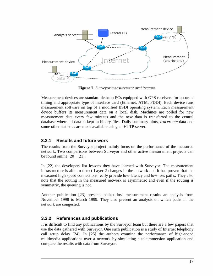
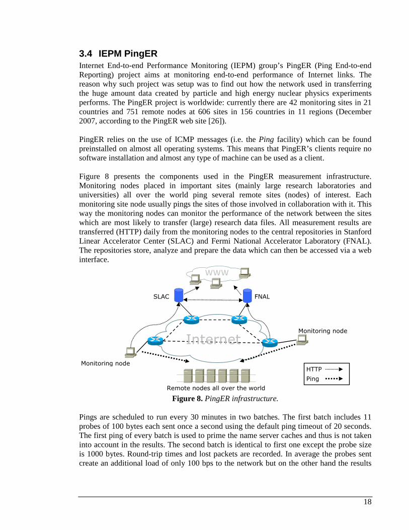
3.4 IEPM PingER Internet End-to-end Performance Monitoring (IEPM) group’s PingER (Ping End-to-end Reporting) project aims at monitoring end-to-end performance of Internet links. The reason why such project was setup was to find out how the network used in transferring the huge amount data created by particle and high energy nuclear physics experiments performs. The PingER project is worldwide: currently there are 42 monitoring sites in 21 countries and 751 remote nodes at 606 sites in 156 countries in 11 regions (December 2007, according to the PingER web site [26]). PingER relies on the use of ICMP messages (i.e. the Ping facility) which can be found preinstalled on almost all operating systems. This means that PingER’s clients require no software installation and almost any type of machine can be used as a client. Figure 8 presents the components used in the PingER measurement infrastructure. Monitoring nodes placed in important sites (mainly large research laboratories and universities) all over the world ping several remote sites (nodes) of interest. Each monitoring site node usually pings the sites of those involved in collaboration with it. This way the monitoring nodes can monitor the performance of the network between the sites which are most likely to transfer (large) research data files. All measurement results are transferred (HTTP) daily from the monitoring nodes to the central repositories in Stanford Linear Accelerator Center (SLAC) and Fermi National Accelerator Laboratory (FNAL). The repositories store, analyze and prepare the data which can then be accessed via a web interface.

Figure 8. PingER infrastructure.

Pings are scheduled to run every 30 minutes in two batches. The first batch includes 11 probes of 100 bytes each sent once a second using the default ping timeout of 20 seconds. The first ping of every batch is used to prime the name server caches and thus is not taken into account in the results. The second batch is identical to first one except the probe size is 1000 bytes. Round-trip times and lost packets are recorded. In average the probes sent create an additional load of only 100 bps to the network but on the other hand the results

SLAC FNAL

Monitoring node

Monitoring node

Remote nodes all over the world

Ping

WWW

Internet

HTTP

19

gained from such sparse sampling are very inaccurate. The use of ICMP packets makes the measurement’s results even more unreliable.

3.4.1 Results and future work In [27] the authors discuss the PingER project and its results. PingER has been successfully used in pointing out needs for network upgrades, tracking network infrastructure changes and illustrating the difference in performance between developed and developing countries. Since PingER uses the ping tool (ICMP Echo Request) to probe the monitored remote-hosts, it suffers from blocking and rate limiting of ICMP packets. According to the authors blocking and rate limiting are increasing, especially in developing countries. This leads to a situation where some of the sites cannot be monitored accurately or at all.

3.4.2 References and publications A report describing the progress of the PingER project can be found in [28]. It lists results from global packet loss and round-trip time measurements and compares these results with economic and development indicators developed by the U.N. and ITU. A selection of publications from the PingER project is available at [29]. These publications focus mainly on the so called Digital Divide. It means the difference between the quality and number of Internet connections available to customers in the developed world and in the developing countries (such as most African countries).

3.5 NLANR AMP Started in 1998 the NLANR’s (National Laboratory for Applied Network Research) Active Measurement Project (AMP) focuses on measuring and analyzing the performance of the network connecting campuses and research sites. The data gathered from the measurements is at the same time used for studying various aspects of Internet traffic. Approximately 150 AMP monitors have been placed around the United States and some strategic sites in other countries to run a full mesh test between all sites. The NLARN project ended in September 2006 and the AMP project was handed over to CAIDA. [30], [31] AMP measures round-trip time, packet loss, topology and throughput between the participating sites. Each monitoring node sends one ICMP packet to each other site in the mesh every minute and records the results. Every 10 minutes a route trace is performed against every other site. AMP allows on-demand throughput tests to be made between any source-destination pair. The tests include bulk TCP and UDP data transfer, ping-F and treno tests. The AMP’s measurement architecture is similar to the PingER architecture. Monitoring nodes run tests between each other and report the results to a central database which processes the data and makes it available for the users via the WWW. AMP’s measurements suffer from the same inaccuracy as the PingER project since it uses ICMP packets and a relatively low sending rate (1 packet per minute). RTT is measured instead

20

of one-way delay because of cost issues: setting up a monitoring network of 100 nodes with GPS receivers is too expensive and difficult to set up.

3.5.1 Results and future work The AMP project has provided researchers, engineers and network designers with valuable data on short and long term network behavior. AMP’s measurement mesh has been used in several studies ([32], [33], [34]) and it has supported a new approach to network measurement, where the net is densely covered with cheap and simple monitors. During the project NLANR researchers have devised a proposal for a new measurement protocol: the IP Measurement Protocol (IPMP). [30], [35] Since the NLANR project has ended and CAIDA has decommissioned most of the AMP probes, there will be no more work done on the project. However, some of the old AMP probes might still be used in other CAIDA projects. [31]

3.5.2 References and publications In [36] the authors present the NLANR project’s Network Analysis Infrastructure which includes the active measurement part (AMP). Hansen et al. present detailed methods to analyze the data gathered with NLANR AMP in [37]. McGregor and Braun discuss and explain the choices they had to make during the NLANR AMP project to balance the cost and quality of the collected data in [38].

3.6 Saturne A more recent (started in 2003) and accurate end-to-end measurement platform is developed by the Saturne project which allows the measurement of IPPM defined one-way delay and packet loss metrics. This measurement platform differs from the previous examples by being mainly located in Europe (France). It has some remote sites in Mexico and South-Korea [39]. Saturne has been used to measure the performance of the French experimental high speed network VTHD. It has also been used to validate (or audit) the DiffServ implementation on the VTHD network and the SLA negotiated by the VTHD. One interesting property of the Saturne platform is that it enables the measurement of different service classes. The Saturne architecture is divided into four separate modules but otherwise it follows the same principles as the Surveyor project:

• Timestamping module: uses GPS to gain accurate timing and ALTQ/ADServ to add DiffServ functionality.

• Emission module: generates the UDP probes. • Capture module: Berkeley Packet Filter based module which receives and analyzes

the probe traffic flows. • Data management module: processes and visualizes the collected data.

All modules run in FreeBSD environment on normal desktop PCs. Data is stored in a mysql database and RRDTool is used as the visualization tool. GPS receivers are

21

connected to the measurement nodes to provide accurate timestamping and packet filters are used to discard unwanted packets before they get to user-space where they only slow down the capturing process. All measuring devices send their results to a central repository by using a Remote Procedure Call (RPC) mechanism. The Saturne architecture is designed to be flexible. All probe emission and class of service parameters are fully configurable meaning that the packet sizes, sending rates and used service classes can be selected to match the needs of any measurement. All the above information and the Saturne architecture are presented in [40].

3.6.1 Results and future work Probably the most notable result of the Saturne project is the verification of the VTHD network QoS policy. Also, the tests done on the Trans-Eurasia Information Network (TEIN) link prove that the connection between France and Korea has a low loss rate and low one-way delay variation [41].

3.6.2 References and publications Very little concerning the Saturne project can be found from the Internet: there does not seem to be too many papers that even mention Saturne. In [40] Corral presents the measurement architecture. The authors in [41] test Saturne for interoperability against another active measurement platform and find that the systems interoperate. They also find that the network connecting the two measurement infrastructures has low loss and low one-way delay variation.

3.7 Comparison between different projects Table 2 gives a brief comparison of the presented projects. L. Cottrell has done a more detailed comparison of Internet active measurement projects and it is available at [42].

Table 2. Comparison between active measurement projects. Project Location Metrics Synchronization Req. Resources

Saturne Europe One-way delay & loss GPS Heavyweight Surveyor Worldwide

(mainly USA)

One-way delay & loss GPS Heavyweight

PingER Worldwide RTT NTP Lightweight NLANR AMP

Worldwide (mainly USA)

RTT NTP Lightweight

NIMI Worldwide (mainly USA)

One-way & loss, Traceroute, bulk transfer throughput etc. (any type of test can be added as a module)

None or NTP (see [16] for details)

Lightweight

22

3.8 Commercial performance measurement products Several commercial performance monitoring products are available [43], [44], [45], [46]. Some products are based on software (agents) that can be installed on normal desktop PCs while other use dedicated measurement hardware. JDSU’s QT-50 and Brix Networks’ Brix Verifier Agent are examples of software measurement agents. Accedian Networks, Prosilient, Brix and JDSU all offer hardware probes for performance measurement. In this thesis Brix Networks’ Brix platform is benchmarked for measurement accuracy. Only the hardware measurement probes are tested as the software measurement agents were not available for testing at the time of this thesis.

3.9 Active application performance measurements Active methods may be used to measure the end-to-end performance of different applications. For example a web server’s performance could be measured by sending probe packets from a host computer across some network. The probe packets used in this case would be normal TCP/IP-packets containing HTTP requests requesting a web page from the server. By sending automated HTTP requests the host is able to measure the time it takes for the server to respond to the requests. Other possible statistics which can be gathered from an HTTP active test include first page download time, first page response time, total download time, redirect time and the network latency. Performance measurements can be done on virtually any application. The most common active performance tests are done on such protocols as HTTP, VoIP, SQL, RSTP, DNS and FTP since these are the most used technologies. Especially VoIP and IPTV tests have become more and more common now that these technologies are coming into widespread use. Enterprises are testing their networks to see how their new VoIP systems perform and operators are testing their capabilities to offer IPTV services for their customers.

3.10 Device performance testing RFC 2544 (and RFC 1242) provides a standardized benchmarking methodology and allows comparing of different vendors’ products such as routers, switches etc. It specifies a set of tests that produce measurement data that can be compared with the results produced by a different vendor’s product. Specified tests include throughput, frame loss, latency and system recovery. All these tests are done with active means i.e. probe traffic is generated and the response of the device under test (DUT) is recorded.

3.11 Active probing in network security Active probing has a special place in computer and network security field as it is used to find security vulnerabilities in networks and hosts (it must be noted here that the same probing tools can, unfortunately, be used for malicious purposes).

23

There are tools that can be used to scan ports and to detect known vulnerabilities on host computers. These tools can often identify software and services running on hosts and also detect the installed operating system(s) and security patches. The operating system (OS) detection (OS fingerprinting) is often based on sending packets to different ports and deducting the OS from the ports that are open. Another way of fingerprinting OSs is to analyze the reactions of the target host’s TCP stack to different TCP packets. Some OSs can be identified from the initial TCP window size alone [47], while others require a bit more sophisticated approach such as interpreting the slight variances in the TCP option fields. When implementing their own versions of the TCP stack, operating system developers follow the TCP RFC (RFC793) and often see it as a recommendation, thus their implementations vary slightly. These variations can be used to detect and fingerprint an operating system. The most well known free network security tools that incorporate some kind of active probing are listed below.

• xProbe (http://sourceforge.net/projects/xprobe/) • hPing (http://www.hping.org/) • Nessus (http://www.nessus.org/) • Nmap (http://insecure.org/nmap/)

A website (http://sectools.org/index.html) lists other useful security tools some of which include active probing components.

3.12 Layer 2 measurements Measurement mechanisms and techniques on the link layer are presented in this section. Traditionally link layer measurement has been minimal, but now as Ethernet technologies are being more widely deployed in the carrier level, Ethernet measurement and troubleshooting tools are becoming more important.

3.12.1 Ethernet OAM Operations, administration and maintenance (OAM) protocols for Ethernet provide operators the same troubleshooting tools for Ethernet that they have been using on the IP layer. These tools include Continuity Check, Link Trace and Loopback Messages. Continuity check (CC) messages are used as a heart beat signal to detect connectivity between two endpoints. Link trace messages are sent to trace a path hop by hop between two endpoints. This is the Ethernet equivalent for the Traceroute tool on IP layer. Loopback message functionality is similar to ICMP Ping. Its function is to test for connectivity between two endpoints. [48]

24

3.12.2 UDLD Unidirectional Link Detection (UDLD) is a Layer 2 mechanism to detect unidirectional Ethernet fiber or copper links but it can also detect for example mis-wirings, interface and media converter faults. A unidirectional link is a situation where a normal bidirectional Ethernet link loses it capability to either transmit or receive data from the Ethernet port at the other end of the link. This kind of fault can cause different types of problems in a network such as spanning-tree topology loops or malfunctioning of other protocols. UDLD monitors the physical configuration of the cables and detects whenever a unidirectional link exists. In case UDLD detects a unidirectional link, it shuts down the affected port and creates an alert for the network administrator. UDLD works with Layer 1 mechanisms to determine a link’s physical status and also to detect the existence of physical and logical unidirectional connections. Autonegotiation is one of these Layer 1 mechanisms: it takes care of physical signaling and fault detection at Layer 1. UDLD performs mutual neighbor identification and neighbor acknowledgement on top of the Logical Link Control (LLC) layer. This makes it possible for UDLD to discover logical one-way mis-communication between neighbors even if a physical layer mechanism has reported the communication to be bidirectional. To be able to detect faults and mis-configurations UDLD uses two mechanisms. The first mechanism is used to advertise a port’s identity with hello-packets and to learn the identities of its neighbors. These identities are kept in a neighbor database for a defined time interval (time-to-live, TTL) after which they are considered old and removed. The second mechanism periodically sends UDLD echo messages to its neighbors’ UDLD enabled ports. If the packets are not echoed back in a specific time, the link is considered unidirectional and the port is shut down. [49]

3.12.3 Link layer (physical) topology discovery Several proprietary solutions to Layer 2-discovery (e.g. Cisco Discovery Protocol) exist. These solutions are device manufacturer dependent and do not work in heterogeneous network environments. There are also some automatic link layer topology discovery algorithms proposed by the research community [50], [51]. There has been some talk in IEEE 802.1 working group to develop a physical topology discovery protocol [52] but nothing has been standardized yet.

3.13 Measurements on Layer 2+ to Layer 4 In this section some well known Layer 2+, Layer 3 and Layer 4 active measurement mechanisms are presented. The list includes mechanisms built into routing hardware, measurement tools developed by the research community and general measurement techniques. Note that here the term “Layer 2+” means that the mechanism or technique is on top of Layer 2 but not on Layer 3 (e.g. MPLS). The mechanisms and methods are presented in such order that lower layer methods are presented first.

25

3.13.1 MPLS/LSP-Ping LSP-Ping [53] is intended as a diagnostic tool for operators to isolate faults in MPLS networks and especially to detect synchronization problems between the data and control planes. It works in two modes: ping mode and traceroute mode. These two modes correspond to the ICMP ping and traceroute tools used in IP networks for connectivity tests (ping), path tracing and fault isolation (traceroute). LSP-Ping’s main use is to verify that packets belonging to a certain FEC really go through the path that they are supposed to. This is done by sending an MPLS Echo Request packet through the same path as all the other packets belonging to this FEC. In ping mode the echo request packets are forwarded just like any other packet in the FEC and once they reach the egress router they are sent to the control plane of the egress router. The control plane checks if the egress router is actually the egress point for the packet’s FEC. In the traceroute mode the echo packets are sent to the control plane of each LSR along the path to see if the LSR is a valid transit LSR for the packet’s intended path. Transit LSRs return information that can be used to check if the forwarding on the router matches what the routing protocols determined as the path for this packet (control plane check against the data plane). MPLS echo request packets are routed based on the label stack so the IP address of the receiving end is never used in the forwarding decision. This means that the sender of the echo request packet does not have to know the IP address of the egress router. To prevent packets from causing confusion in the network in case of LSP failure, the destination IP address should be selected from the 127/8 address range (internal host loopback address, localhost) [54]. This way the packets that happen to drop out from the LSP are not IP forwarded but are silently discarded instead [55].

3.13.2 Juniper Real-time Performance Monitor (RPM) RPM [56] is an active measurement mechanism built into Juniper routers to actively monitor the performance of network paths between two or more Juniper devices. By sending a constant flow of probes routers can monitor for example the level of delay inside a VPN. Main use for RPM is performance monitoring on Layers 3 and 4 and it can also be used to generate SNMP traps on SLA violations. So, for example if the delay level inside a VPN rises above some predetermined value, then an alarm is generated. Alarm generating thresholds can be configured so that the monitoring and analysis of the measurement results are simplified. All results can be directly used from the CLI, fetched via SNMP or exported to external network management applications. RPM supports RFC 2925 MIB (Management Information Base) with extensions. The RFC defines a MIB for performing remote ping, traceroute and IP or DNS lookup operations at remote hosts meaning that a Juniper router can be used to initiate one of the mentioned operations on another Juniper router.

26

The following types of probes are supported by RPM with Differentiated Services Code Point (DSCP) marking:

• ICMP Echo • ICMP Timestamp • HTTP Get • UDP Echo • TCP Connection

The probe packets can be given a priority over regular data packets on input interfaces in which case the probes can reach their destination even if there is congestion. Such results as minimum, maximum and average round-trip time, RTT delay variation and standard deviation, number of probes sent and percentage of lost probes are produced by the probes.

3.13.3 Cisco Service Assurance Agent / IOS IP Service Level Agreements

Formerly known as the Service Assurance Agent (SAA) the Cisco IOS IP SLAs [57] is much like its Juniper counterpart RPM. It is a built in feature of the Cisco IOS devices allowing active probing and thus active monitoring. The probes have several configurable options such as UDP/TCP port numbers, ToS field, VRF instance, source and destination IP addresses and web URL. Since IP SLAs is Layer 2 transport independent it can be configured to run end-to-end over a heterogeneous network. IP SLAs allow the collection of the following performance metrics:

• One-way delay • Round-trip delay • Delay variation • Packet loss • Packet ordering • Voice quality scoring • Network resource availability • Application performance • Server response time

The data collected by the probes can be accessed via CLI or SNMP MIBs and it can be used by third party performance monitoring applications.

3.13.4 Active network layer topology discovery With the speed networks are growing and changing today getting a clear picture of a network’s topology is becoming more and more difficult. Topology information is valuable for network resource managers and administrators planning server placements.

27

Researchers also need topology information to simulate networks. Different tools and methods have been proposed for active network topology discovery [58], [59], [60]. Most of these tools are based on SNMP or traceroute-like methods (sending hop-limited packets to a destination address and waiting for an ICMP message indicating IP TTL expiration).

3.13.5 Reachability / Ping One of the most basic active network measurements is testing if a certain host is reachable (available). This can be done easily by sending an ICMP echo_request (ICMP Type 8) packet to the target host which then elicits an ICMP echo_response. The most well known reachability testing tool is the ping tool originally written by Mike Muuss in 1983. Its usefulness and simplicity has allowed it to rise to a status where it is built in to nearly every operating system. In addition to measuring reachability ping can also be used to estimate (measure) round-trip delay and packet-loss. Even ping has its problems. Many ISPs have begun to filter out ICMP echo requests because of growing number of Internet worms using them to search for potential targets. Also, some hosts do not reply to echo requests in purpose to hide their presence. These facts diminish the usefulness of the ping tool, but most of the time it still is the most valuable tool a network engineer has when performing troubleshooting.

3.13.6 Route discovery / Traceroute Finding out what route a packet takes on its way through a network can be done by exploiting the time-to-live (TTL) field of the IP header. The TTL field on an IP packet is decremented every time the packet is processed by a router. When the TTL counter of an IP packet reaches zero, the packet is dropped and an ICMP TTL Expired –message is sent back to the sender. By sending packets with increasing TTL fields (starting from 1) each router on the path can be elicited to send an expiration message thus all routers can be identified. The method described here was first used in the famous traceroute program written by Van Jacobson [61]. Known problems exist in the traceroute method as presented by Vern Paxson in [62]:

• The method assumes that all intermediate routers send ICMP messages while this is not true in all cases as some routers are configured not to send or reply to ICMP messages because of security concerns

• Layer 2 devices are transparent to the method: switches and different link layer technologies cannot be discovered with traceroute

The traceroute tool is similar to the ping tool in its popularity as it is built in to most of the current operating systems. Unfortunately, it suffers even more than ping from the filtering issues since not all routers reply to ICMP messages. Often traceroute returns only the first few routers on the path.

28

3.13.7 Path MTU discovery The largest packet size that can be sent on to a link without fragmenting the packet is called the Maximum Transmission Unit (MTU). An arbitrary path between two nodes in a network may have links that have different MTUs. The smallest MTU on the path between these two nodes is the Path MTU (PMTU). When sending large amounts of data across a network it is efficient to use the largest MTU possible; using a smaller packet size would waste resources. RFC 1191 [63] defines one ICMP based Path MTU discovery mechanism. This mechanism has several problems which are discussed in RFC 2923 [64]. The mechanism defined in RFC 1191 uses the IP header’s Don’t Fragment bit to discover the PMTU of a path. A source node first assumes that the PMTU is the MTU of the first hop. With the DF bit set in every packet, the node starts to send traffic to the destination node. If a router on the path notices that the datagram cannot be sent to a next hop without fragmentation, the router drops the packet and sends an ICMP Destination Unreachable message with the code “fragmentation needed and DF set” back to the source node [65]. When a source node receives these messages, it automatically reduces the size of the packets and thus the PMTU until it receives no more error messages. However, the source must never reduce its PMTU estimate below 68 octets, since, according to RFC 791, every router must be able to send packets of 68 bytes without fragmenting them. [63] Increases in the PMTU can be detected by periodically sending packets with increased PMTU (e.g. by setting the PMTU back to the MTU of the first hop). Since this will most likely result in more of above mentioned ICMP messages, it is recommended that the testing is done infrequently. Decreases of the PMTU are detected by ICMP “fragmentation needed and DF set” messages.

3.13.8 Available bandwidth measurement methods and tools Some applications benefit from knowing the amount of bandwidth available on a network path so that they can adapt their sending rate and share the bandwidth more fairly. Such applications include multimedia content adaptation, dynamic server selection, peer-to-peer applications and congestion control transports. Measuring (or rather, estimating) available bandwidth with active probing is required when all routers along a network path are not controlled by the measurer (passive measurement methods cannot be used). When measuring available bandwidth by probing, it must be noted that all current methods merely give approximations of the current bandwidth usage of a path. The available methods used are not very accurate especially when used to measure high bandwidth links [6]. There are four major techniques that are used when estimating available bandwidth. A brief overview of these techniques is given here; a more thorough review can be found for example in [6]. 1. Variable Packet Size (VPS) technique attempts to estimate the capacity of each link (hop) along a path. VPS does this by sending different sized probe packets from the source

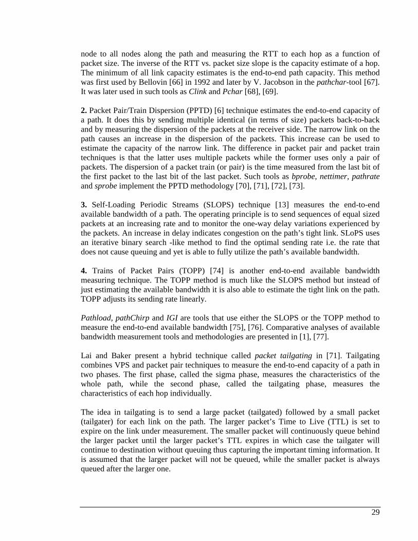
29

node to all nodes along the path and measuring the RTT to each hop as a function of packet size. The inverse of the RTT vs. packet size slope is the capacity estimate of a hop. The minimum of all link capacity estimates is the end-to-end path capacity. This method was first used by Bellovin [66] in 1992 and later by V. Jacobson in the pathchar-tool [67]. It was later used in such tools as Clink and Pchar [68], [69]. 2. Packet Pair/Train Dispersion (PPTD) [6] technique estimates the end-to-end capacity of a path. It does this by sending multiple identical (in terms of size) packets back-to-back and by measuring the dispersion of the packets at the receiver side. The narrow link on the path causes an increase in the dispersion of the packets. This increase can be used to estimate the capacity of the narrow link. The difference in packet pair and packet train techniques is that the latter uses multiple packets while the former uses only a pair of packets. The dispersion of a packet train (or pair) is the time measured from the last bit of the first packet to the last bit of the last packet. Such tools as bprobe, nettimer, pathrate and sprobe implement the PPTD methodology [70], [71], [72], [73]. 3. Self-Loading Periodic Streams (SLOPS) technique [13] measures the end-to-end available bandwidth of a path. The operating principle is to send sequences of equal sized packets at an increasing rate and to monitor the one-way delay variations experienced by the packets. An increase in delay indicates congestion on the path’s tight link. SLoPS uses an iterative binary search -like method to find the optimal sending rate i.e. the rate that does not cause queuing and yet is able to fully utilize the path’s available bandwidth. 4. Trains of Packet Pairs (TOPP) [74] is another end-to-end available bandwidth measuring technique. The TOPP method is much like the SLOPS method but instead of just estimating the available bandwidth it is also able to estimate the tight link on the path. TOPP adjusts its sending rate linearly. Pathload, pathChirp and IGI are tools that use either the SLOPS or the TOPP method to measure the end-to-end available bandwidth [75], [76]. Comparative analyses of available bandwidth measurement tools and methodologies are presented in [1], [77]. Lai and Baker present a hybrid technique called packet tailgating in [71]. Tailgating combines VPS and packet pair techniques to measure the end-to-end capacity of a path in two phases. The first phase, called the sigma phase, measures the characteristics of the whole path, while the second phase, called the tailgating phase, measures the characteristics of each hop individually. The idea in tailgating is to send a large packet (tailgated) followed by a small packet (tailgater) for each link on the path. The larger packet’s Time to Live (TTL) is set to expire on the link under measurement. The smaller packet will continuously queue behind the larger packet until the larger packet’s TTL expires in which case the tailgater will continue to destination without queuing thus capturing the important timing information. It is assumed that the larger packet will not be queued, while the smaller packet is always queued after the larger one.

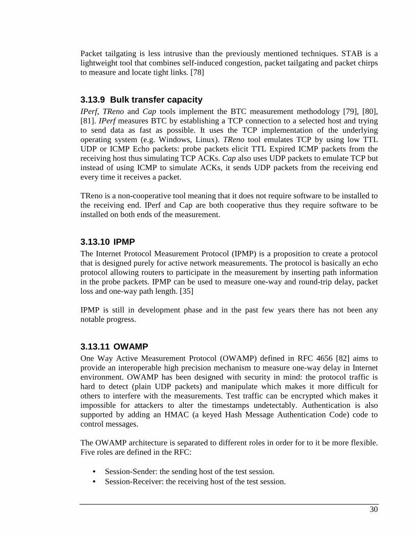
30

Packet tailgating is less intrusive than the previously mentioned techniques. STAB is a lightweight tool that combines self-induced congestion, packet tailgating and packet chirps to measure and locate tight links. [78]

3.13.9 Bulk transfer capacity IPerf, TReno and Cap tools implement the BTC measurement methodology [79], [80], [81]. IPerf measures BTC by establishing a TCP connection to a selected host and trying to send data as fast as possible. It uses the TCP implementation of the underlying operating system (e.g. Windows, Linux). TReno tool emulates TCP by using low TTL UDP or ICMP Echo packets: probe packets elicit TTL Expired ICMP packets from the receiving host thus simulating TCP ACKs. Cap also uses UDP packets to emulate TCP but instead of using ICMP to simulate ACKs, it sends UDP packets from the receiving end every time it receives a packet. TReno is a non-cooperative tool meaning that it does not require software to be installed to the receiving end. IPerf and Cap are both cooperative thus they require software to be installed on both ends of the measurement.

3.13.10 IPMP The Internet Protocol Measurement Protocol (IPMP) is a proposition to create a protocol that is designed purely for active network measurements. The protocol is basically an echo protocol allowing routers to participate in the measurement by inserting path information in the probe packets. IPMP can be used to measure one-way and round-trip delay, packet loss and one-way path length. [35] IPMP is still in development phase and in the past few years there has not been any notable progress.

3.13.11 OWAMP One Way Active Measurement Protocol (OWAMP) defined in RFC 4656 [82] aims to provide an interoperable high precision mechanism to measure one-way delay in Internet environment. OWAMP has been designed with security in mind: the protocol traffic is hard to detect (plain UDP packets) and manipulate which makes it more difficult for others to interfere with the measurements. Test traffic can be encrypted which makes it impossible for attackers to alter the timestamps undetectably. Authentication is also supported by adding an HMAC (a keyed Hash Message Authentication Code) code to control messages. The OWAMP architecture is separated to different roles in order for to it be more flexible. Five roles are defined in the RFC:

• Session-Sender: the sending host of the test session. • Session-Receiver: the receiving host of the test session.

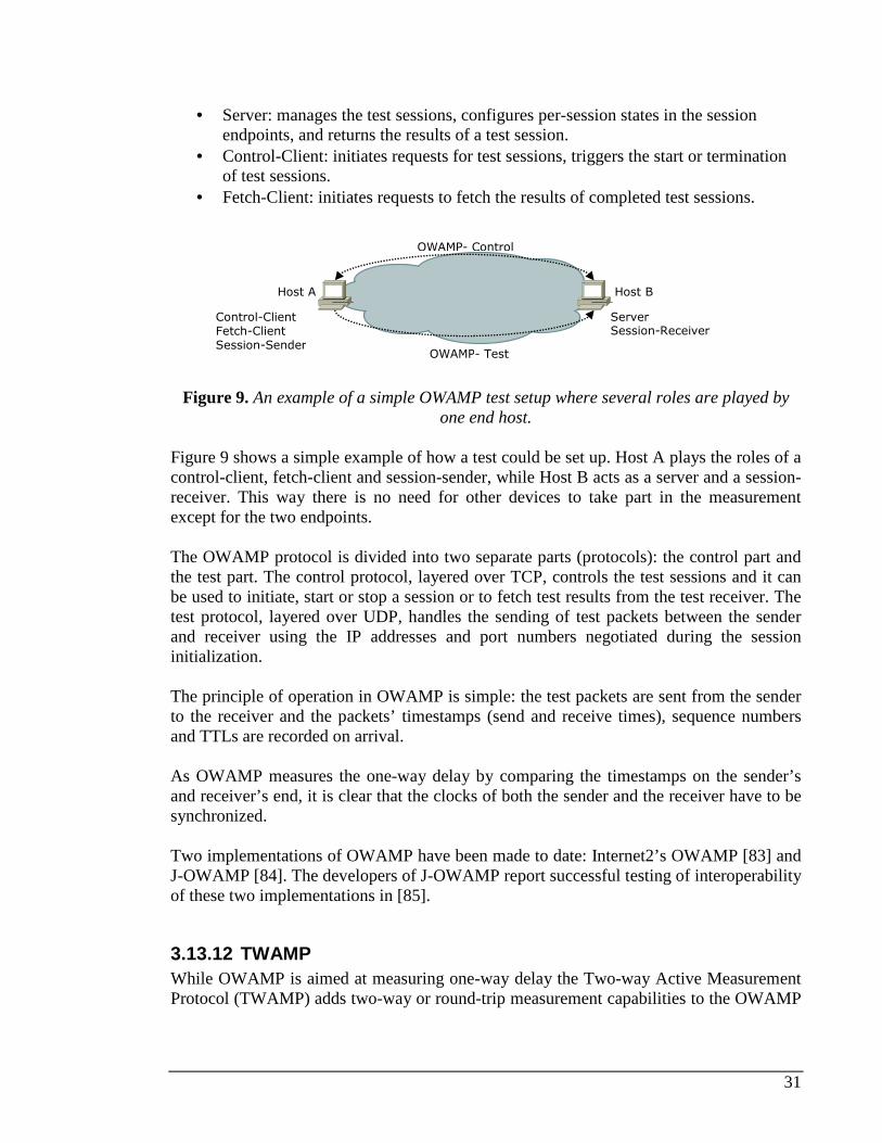
31

• Server: manages the test sessions, configures per-session states in the session endpoints, and returns the results of a test session.

• Control-Client: initiates requests for test sessions, triggers the start or termination of test sessions.

• Fetch-Client: initiates requests to fetch the results of completed test sessions.

Figure 9. An example of a simple OWAMP test setup where several roles are played by

one end host. Figure 9 shows a simple example of how a test could be set up. Host A plays the roles of a control-client, fetch-client and session-sender, while Host B acts as a server and a session-receiver. This way there is no need for other devices to take part in the measurement except for the two endpoints. The OWAMP protocol is divided into two separate parts (protocols): the control part and the test part. The control protocol, layered over TCP, controls the test sessions and it can be used to initiate, start or stop a session or to fetch test results from the test receiver. The test protocol, layered over UDP, handles the sending of test packets between the sender and receiver using the IP addresses and port numbers negotiated during the session initialization. The principle of operation in OWAMP is simple: the test packets are sent from the sender to the receiver and the packets’ timestamps (send and receive times), sequence numbers and TTLs are recorded on arrival. As OWAMP measures the one-way delay by comparing the timestamps on the sender’s and receiver’s end, it is clear that the clocks of both the sender and the receiver have to be synchronized. Two implementations of OWAMP have been made to date: Internet2’s OWAMP [83] and J-OWAMP [84]. The developers of J-OWAMP report successful testing of interoperability of these two implementations in [85].

3.13.12 TWAMP While OWAMP is aimed at measuring one-way delay the Two-way Active Measurement Protocol (TWAMP) adds two-way or round-trip measurement capabilities to the OWAMP

Host A Host B

Control-Client Fetch-Client Session-Sender

Server Session-Receiver

OWAMP- Control

OWAMP- Test

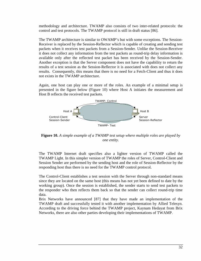
32

methodology and architecture. TWAMP also consists of two inter-related protocols: the control and test protocols. The TWAMP protocol is still in draft status [86]. The TWAMP architecture is similar to OWAMP’s but with some exceptions. The Session-Receiver is replaced by the Session-Reflector which is capable of creating and sending test packets when it receives test packets from a Session-Sender. Unlike the Session-Receiver it does not collect any information from the test packets as round-trip delay information is available only after the reflected test packet has been received by the Session-Sender. Another exception is that the Server component does not have the capability to return the results of a test session as the Session-Reflector it is associated with does not collect any results. Consequently, this means that there is no need for a Fetch-Client and thus it does not exists in the TWAMP architecture. Again, one host can play one or more of the roles. An example of a minimal setup is presented in the figure below (Figure 10) where Host A initiates the measurement and Host B reflects the received test packets.

Figure 10. A simple example of a TWAMP test setup where multiple roles are played by

one entity. The TWAMP Internet draft specifies also a lighter version of TWAMP called the TWAMP Light. In this simpler version of TWAMP the roles of Server, Control-Client and Session Sender are performed by the sending host and the role of Session-Reflector by the responding host thus there is no need for the TWAMP control protocol. The Control-Client establishes a test session with the Server through non-standard means since they are located on the same host (this means has not yet been defined to date by the working group). Once the session is established, the sender starts to send test packets to the responder who then reflects them back so that the sender can collect round-trip time data. Brix Networks have announced [87] that they have made an implementation of the TWAMP draft and successfully tested it with another implementation by Allied Telesyn. According to the driving force behind the TWAMP project, Kaynam Hedayat from Brix Networks, there are also other parties developing their implementations of TWAMP.

Host A Host B

Control-Client Session-Sender

Server Session-Reflector

TWAMP- Control

TWAMP- Test

33

3.14 BFD-protocol The goal of Bidirectional Forwarding Detection (BFD) protocol is to test for path failures between any two adjacent network nodes’ forwarding engines. BFD works independently of media, data protocols and routing protocols. Another of its goals is to provide liveness detection over any media and at any protocol layer without the need of multiple methods. [88]

3.14.1 Operating modes BFD can be used in two different operating modes: asynchronous and demand modes. In the former mode, which is the primary mode, BFD control packets are periodically sent between the two systems. If a system stops receiving packets for a certain time, the path, or some part of the path, is assumed failed. This way BFD is very similar to IGP HELLO-protocols. In the latter operating mode, it is assumed that the systems verify the connectivity to the other system by some other means (e.g. by receiving traffic from the remote system). The systems stop sending control packets after the BFD session is established and only send packets when they feel there is an explicit need to verify the connectivity (e.g. after a period of silence between two systems). BFD has a third optional operation mode that can be used with the two modes mentioned above. This third mode is known as the Echo function. The echo function forces the remote system to loop back all the BDF echo packets sent by a system thus exercising the entire forwarding path in the remote system. By using the Echo function the rate of control packets can be reduced in asynchronous mode or eliminated completely in the demand mode. This is because the Echo function is handling the task of detection.

3.14.2 Applications for BFD Since BFD can be run on any protocol layer, the semantics of a session break down is in context of the protocol used to encapsulate the BFD packets. For example the breakdown of a BFD-over-IP session implies an IGP neighbor failure (IGP neighborhood should be removed) and the breakdown of a BDF-over-Ethernet session implies a switch failure [89]. BFD can be used in one-hop or multi-hop situations [90], [91] and it can also be used to detect MPLS LSP data plane failures [92]. This means that BFD sessions can be established over direct physical links, virtual circuits, tunnels, LSPs or even OSPF virtual links. A separate BFD session has to be set up for each individual protocol or link between two systems. BFD can be used to complement MPLS LSP-Ping for faster detection of MPLS data plane failures. While LSP-Ping is somewhat heavy on the control plane processors, BFD packet processing is relatively lighter and more suitable for hardware or firmware implementations. Since BFD is lighter it means that it can support fault detection for greater number of LSPs. Also, BFD is designed to detect faults with sub-second

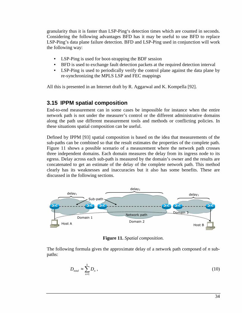
34

granularity thus it is faster than LSP-Ping‘s detection times which are counted in seconds. Considering the following advantages BFD has it may be useful to use BFD to replace LSP-Ping’s data plane failure detection. BFD and LSP-Ping used in conjunction will work the following way:

• LSP-Ping is used for boot-strapping the BDF session • BFD is used to exchange fault detection packets at the required detection interval • LSP-Ping is used to periodically verify the control plane against the data plane by

re-synchronizing the MPLS LSP and FEC mappings All this is presented in an Internet draft by R. Aggarwal and K. Kompella [92].

3.15 IPPM spatial composition End-to-end measurement can in some cases be impossible for instance when the entire network path is not under the measurer’s control or the different administrative domains along the path use different measurement tools and methods or conflicting policies. In these situations spatial composition can be useful. Defined by IPPM [93] spatial composition is based on the idea that measurements of the sub-paths can be combined so that the result estimates the properties of the complete path. Figure 11 shows a possible scenario of a measurement where the network path crosses three independent domains. Each domain measures the delay from its ingress node to its egress. Delay across each sub-path is measured by the domain’s owner and the results are concatenated to get an estimate of the delay of the complete network path. This method clearly has its weaknesses and inaccuracies but it also has some benefits. These are discussed in the following sections.

Figure 11. Spatial composition.

The following formula gives the approximate delay of a network path composed of n sub-paths:

∑=

≈k

nntotal DD

1

, (10)

Host A Host B

Domain 1

Domain 2

Domain 3

delay1

delay2

delay3

Network path

Sub-path

35

where k is the number of sub-paths, Dn the delay of a sub-path and Dtotal the combined delay of all sub-paths. IPPM has defined spatial composition metrics also for packet loss and delay variation.

3.15.1 Justification It may sometimes be more practical to run only few well placed measurements between the edges of a domain rather than to run a large amount of measurements across the domain. For example, a service provider whose clients constantly run measurements to determine their quality of service across the provider’s network could benefit from running a measurement between its edge routers. The results from the measurement could be used by all the clients so that they would not have to run their own measurements.

3.15.2 Accuracy and sources of error Since the inter-domain measurement packets have their source and destination addresses set to those of the domain’s edge routers instead of the addresses of the complete path’s source and destination, the packets may actually travel a different route across the domain. This may cause the results to differ from the results gained by measuring the complete path.

3.15.3 Spatial decomposition The opposite of spatial composition is spatial decomposition. The idea is to measure a complete path and then try to deduce how much each sub-path contributed to the result of the measurement. For example, when measuring delay of a complete network path, the delay of a sub-path can be estimated by using spatial decomposition.

36

Chapter 4

Active measurement challenges Active network measurements face several challenges. In this chapter some of the major challenges are presented and discussed. The fundamental questions are: how many probes are needed to accurately measure delay or packet loss, what is the time required for an accurate measurement, and how accurate the current measurement methods really are? Active probing can overload the network causing congestion especially when there already is a high load on the network. This is a problem because usually the most accurate performance measurements are needed when the network is highly loaded.

4.1 Measurement protocols UDP, TCP and ICMP protocols were not designed to be used for measurements so they do not suit well for the modern Internet. New protocols have been proposed for this purpose. Such protocols are the Internet Protocol Measurement Protocol (IPMP), One-way Active Measurement Protocol (OWAMP) and Two-way Active Measurement Protocol (TWAMP). These new protocols are mainly used for setting up and controlling measurement sessions and use UDP or other “old” protocols to carry the actual measurement traffic.

4.2 Sampling The discrete sampling nature of probing is probably the active measurement’s greatest problem. By probing a network, one can only sample the state of the network. Selecting the interval at which the probe packets are sent to the network is important: the characteristics of the sampling process affect the accuracy of the measurement. Traditionally probes have been sent with Poisson-modulated intervals according to the well known PASTA principle (Poisson Arrivals See Time Averages) [94], but some recent work questions the usefulness of PASTA. In [95] the authors claim that Poisson probing is rarely required and propose an alternative default for probes and probing patterns. The IPPM framework [5] suggests the use of PASTA for Internet measurements but also comments that there are situations where other probe distributions may be better.

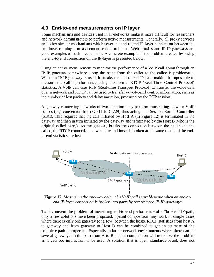
37

4.3 End-to-end measurements on IP layer Some mechanisms and devices used in IP-networks make it more difficult for researchers and network administrators to perform active measurements. Generally, all proxy services and other similar mechanisms which sever the end-to-end IP-layer connection between the end hosts running a measurement, cause problems. Web-proxies and IP-IP gateways are good examples of such mechanisms. A concrete example of the problem created by losing the end-to-end connection on the IP-layer is presented below. Using an active measurement to monitor the performance of a VoIP call going through an IP-IP gateway somewhere along the route from the caller to the callee is problematic. When an IP-IP gateway is used, it breaks the end-to-end IP path making it impossible to measure the call’s performance using the normal RTCP (Real-Time Control Protocol) statistics. A VoIP call uses RTP (Real-time Transport Protocol) to transfer the voice data over a network and RTCP can be used to transfer out-of-band control information, such as the number of lost packets and delay variation, produced by the RTP session. A gateway connecting networks of two operators may perform transcoding between VoIP codecs (e.g. conversion from G.711 to G.729) thus acting as a Session Border Controller (SBC). This requires that the call initiated by Host A (in Figure 12) is terminated in the gateway and then in turn initiated by the gateway and terminated by the Host B (who is the original called party). As the gateway breaks the connection between the caller and the callee, the RTCP connection between the end hosts is broken at the same time and the end-to-end statistics are lost.

Figure 12. Measuring the one-way delay of a VoIP call is problematic when an end-to-

end IP-layer connection is broken into parts by one or more IP-IP-gateways. To circumvent the problem of measuring end-to-end performance of a “broken” IP-path, only a few solutions have been proposed. Spatial composition may work in simple cases where there is only one gateway (or a few) between the hosts. RTCP statistics from host A to gateway and from gateway to Host B can be combined to get an estimate of the complete path’s properties. Especially in larger network environments where there can be several gateways on the path from A to B spatial composition will not solve the problem as it gets too impractical to be used. A solution that is open, standards-based, does not

Host A

Host B

IP-IP gateway

Network A

VoIP traffic

Network B

Border between two operators

38

require any changes in the existing devices, and does not rely on vendor implementations has to be found. One such solution could be to insert a timestamp (in case of one-way delay measurement) in the payload data of the RTP packet since it is the only part of a VoIP data packet that remains the same when an SBC is placed on the path. This approach gets more difficult if transcoding is performed to the voice stream somewhere along the path since it will most likely scramble the timestamp so that the information is uninterpretable once it reaches the receiving end. In this case the timestamp has to be selected is such a way that the transcoding does not affect it. One way could be to Fourier transform the selected timestamp at Host A and then take an inverse transformation of the data on Host B. This way the transcoding process should not affect the timestamp.

4.4 Measuring packet loss Packet loss can have a substantial impact on several Internet protocols and applications. TCP suffers from packet loss since it temporarily drops its sending rate if a packet is lost. Although TCP interprets the lost packet as a sign of congestion there might be another reason for the packet to be lost e.g. a random bit error on the physical layer. Another issue with TCP-connections is that while they suffer from data packet loss, they can also suffer from the loss of TCP Acknowledgement packets (ACK loss). Real-time media applications using UDP do not suffer from single lost packets as the packets usually contain only a very small portion of the total video or audio stream. Also, UDP protocol does not suffer from ACK losses as the protocol is connectionless. When packet loss rate becomes higher, it starts to affect also streaming media making a video stream garbled. A packet loss of only 1 % can significantly reduce the quality of a VoIP call. A lost route advertisement message will cause a network to converge slower because the lost packet has to be re-sent and there might even be a timer that has to expire before it can be done. Several things have to be considered when measuring packet loss:

• When can a packet be declared to be lost? • What is the sufficient length of a packet loss measurement? • How many probes are required for an accurate measurement?

If we consider packet delay distribution in Figure 13 we can see that the tail of the distribution graph is long. As the tail can, in theory, be infinitely long there is a need to specify some bound to what the delay can be before a packet is considered to be lost. The delay bound depends on the application e.g. in a VoIP application it is usually better to discard a single late packet than to stop playing the audio stream while waiting for it. A large file transfer on the other hand can afford to wait for a single packet a bit longer before re-sending it because the file (usually) cannot be used before all the data packets have arrived to the destination. This way the receiver does not suffer from waiting for a single packet as it can transfer the other remaining packets while waiting for the missing

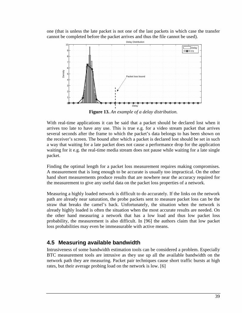
39

one (that is unless the late packet is not one of the last packets in which case the transfer cannot be completed before the packet arrives and thus the file cannot be used).

0

1

2

3

4

5

6

7

8

9

10

Delay

Den

sity

Delay Distribution

DelayFit

Packet loss bound

Figure 13. An example of a delay distribution.

With real-time applications it can be said that a packet should be declared lost when it arrives too late to have any use. This is true e.g. for a video stream packet that arrives several seconds after the frame to which the packet’s data belongs to has been shown on the receiver’s screen. The bound after which a packet is declared lost should be set in such a way that waiting for a late packet does not cause a performance drop for the application waiting for it e.g. the real-time media stream does not pause while waiting for a late single packet. Finding the optimal length for a packet loss measurement requires making compromises. A measurement that is long enough to be accurate is usually too impractical. On the other hand short measurements produce results that are nowhere near the accuracy required for the measurement to give any useful data on the packet loss properties of a network. Measuring a highly loaded network is difficult to do accurately. If the links on the network path are already near saturation, the probe packets sent to measure packet loss can be the straw that breaks the camel’s back. Unfortunately, the situation when the network is already highly loaded is often the situation when the most accurate results are needed. On the other hand measuring a network that has a low load and thus low packet loss probability, the measurement is also difficult. In [96] the authors claim that low packet loss probabilities may even be immeasurable with active means.

4.5 Measuring available bandwidth Intrusiveness of some bandwidth estimation tools can be considered a problem. Especially BTC measurement tools are intrusive as they use up all the available bandwidth on the network path they are measuring. Packet pair techniques cause short traffic bursts at high rates, but their average probing load on the network is low. [6]

40

Many of the more sophisticated bandwidth measurement techniques, such as the packet-pair method, give accurate results in only under certain conditions. Some tools can be used without the need of administering both the source and destination nodes. Other methods rely on accurate timing on both ends of the measurement path and this often means that tester needs some control over the destination host. Packet pair techniques usually require that measurement software is running on both ends of the network path. Some mechanisms, such as VPS probing, use ICMP replies to gather delay data from routers along the measured path. This is a problem because (as mentioned before) ICMP messages are often not processed with the same priority as normal traffic and this way the resulting measurements are inaccurate. One good example of this is the traceroute tool which rarely displays the complete path if run between two hosts connected via Internet. In addition to the ICMP problem, VPS probing method suffers from a problem that may cause it to severely underestimate the available capacity of a path. The VPS method assumes that each hop of a path adds to the one-way delay of a probe packet by a serialization latency, which can be calculated as the ratio of the probe size over the hop’s capacity. Layer 2 devices do not send the ICMP Time Exceeded messages required for the VPS method to calculate the capacity estimate, but they add serialization delays that are not visible to the VPS method. This leads to the VPS method underestimating the capacity of a hop. [97] Cross traffic is a problem for packet-pair methods. The selection of the probe size can affect the amount of error caused by cross traffic. Larger probe size leads to wider gaps between probes. The longer the time between two successive probe packets the greater the possibility that a cross traffic arrives at a router between the two probes and interferes with the measurement. On the other hand, if the packet is very small the results are often overestimated. [98] Packet tailgating method avoids the need of using ICMP messages but it still produces inaccurate results possibly because small errors in link estimation accumulate along the measurement path. It is unable to measure a very fast link after a very slow link and queuing anywhere along the path disrupts the measurements of all links on the path. [71]

4.6 Measuring delay Packet delay measurements play an important role when making network’s capacity planning decisions, tuning applications and detecting faults in networks. Delay of a network path or a link can be measured by either passively monitoring packets traveling the path (link) or by creating active traffic on the path (link). Passive monitoring requires that a packet is recognized and captured in both endpoints (e.g. customer’s CE routers monitor a flow of packets between two VPN sites). Active probing creates a stream of packets that are timestamped at both ends (e.g. a pair of synchronized hosts send UDP packets).

41

4.6.1 Timestamping and synchronization Delay measurements are based on comparing timestamps of test packets. Timestamping means that the exact time the packet arrives (or departs) is recorded and attached to the packet. If packets are timestamped on departure and on arrival, then these two timestamps can be compared to calculate the time it takes for the packet to travel from the source to the destination. The resulting time difference is called the measured delay. In case the clocks in both endpoints are perfectly synchronized (theoretical situation), then the measured delay is the true delay. [99] When making network traffic traces, timestamping arriving packets allows correlating an arriving packet with other arriving packets thus making it possible to calculate several performance metrics such as delay, delay variation, application performance and flow throughput. In multipoint measurements it is especially important to have as accurate timestamps as possible so that a packet’s path through the network can be traced and different events in the network can be correlated. Since delay (and delay variation) measurements are based on the difference between the time the packet was sent and the time the packet was received, it is important that the clocks of both endpoints are synchronized. On today’s high speed network this is becoming more and more challenging as the packets arrive on interfaces on ever increasing frequency. This means that the clocks on the capturing devices need to have an increasingly better resolution. Assuming that the delay measurements are made over some arbitrary network path (e.g. Internet) there are three well known methods available for endpoint synchronization:

• GPS • CDMA • NTP

All these methods use an outside time source to provide synchronization for the endpoints. Above mentioned methods are discussed in more detail below.

4.6.2 GPS The Global Positioning System (GPS) is a global satellite navigation system which allows a GPS receiver to accurately determine its location anywhere on Earth. While the GPS system is mainly used for positioning, it can also be used in telecommunications because the system provides an accurate time reference: GPS satellites have atomic clocks which are extremely precise. [100] GPS receivers suitable for synchronizing usually output a PPS-signal (Pulse per Second) which can be used to discipline the system clock to a very high degree of precision (typically less than 10 µs). A PPS signal is a series of pulses each pulse having logical true and logical false phases. PPS-signal level is triggered every time the UTC-second changes.

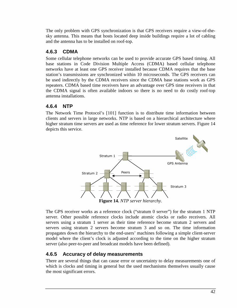
42

The only problem with GPS synchronization is that GPS receivers require a view-of-the-sky antenna. This means that hosts located deep inside buildings require a lot of cabling and the antenna has to be installed on roof-top.

4.6.3 CDMA Some cellular telephone networks can be used to provide accurate GPS based timing. All base stations in Code Division Multiple Access (CDMA) based cellular telephone networks have at least one GPS receiver installed because CDMA requires that the base station’s transmissions are synchronized within 10 microseconds. The GPS receivers can be used indirectly by the CDMA receivers since the CDMA base stations work as GPS repeaters. CDMA based time receivers have an advantage over GPS time receivers in that the CDMA signal is often available indoors so there is no need to do costly roof-top antenna installations.

4.6.4 NTP The Network Time Protocol’s [101] function is to distribute time information between clients and servers in large networks. NTP is based on a hierarchical architecture where higher stratum time servers are used as time reference for lower stratum servers. Figure 14 depicts this service.

Figure 14. NTP server hierarchy. The GPS receiver works as a reference clock (“stratum 0 server”) for the stratum 1 NTP server. Other possible reference clocks include atomic clocks or radio receivers. All servers using a stratum 1 server as their time reference become stratum 2 servers and servers using stratum 2 servers become stratum 3 and so on. The time information propagates down the hierarchy to the end-users’ machines following a simple client-server model where the client’s clock is adjusted according to the time on the higher stratum server (also peer-to-peer and broadcast models have been defined).

4.6.5 Accuracy of delay measurements There are several things that can cause error or uncertainty to delay measurements one of which is clocks and timing in general but the used mechanisms themselves usually cause the most significant errors.

Stratum 1

Stratum 2

Stratum 3

Satellite

GPS Antenna

Peers

43

Asymmetric paths can also cause problems when measuring delay. One cannot simply divide a round-trip time by two to get the delay from A to B and from B to A. The path from A to B can be very different from the path from B to A thus the delay experienced by the probes is not necessarily the same. The type of probe packet used in a measurement must be carefully selected. Different types of packets receive different kind of service in routers along the network path. For example, if ICMP-packets are used to measure delay, there is a danger that the measurement overestimates the delay because ICMP-packets are often given a lower priority in routers than ‘normal’ traffic (i.e. TCP and UDP). The size of the probe packet can also affect the delay experienced by the probes. Selecting the size of the probe packet must be done carefully: on a highly loaded path 64 byte probes will surely produce different results than 1500 byte probes.

4.6.6 Error and uncertainty caused by clocks Timing is one of the major issues in accurate delay measurement. Many active measurement techniques require that the end-hosts running the measurement have their clocks in synchronization. The problem with clocks is that it is difficult to get two clocks to run in same time for the duration of the measurement. These timing issues are discussed in RFC 2679 [102] for a one-way delay metric and in RFC 2681 [103] for a RTT delay metric. Several parameters are related to clock uncertainty:

• Accuracy: tells how close to ‘real time’ (UTC time) the clock is. • Resolution: a measure of how precise the clock is (how often the clock ticks) • Skew: measures the change of accuracy, or of synchronization, with time (e.g. a

clock might gain 1 ms per hour). • Synchronization error (offset): a measure of how well two clocks agree on what

time is.

These parameters are used in identifying the uncertainties or errors clocks cause when measuring delay. Both clocks, on the sending and the receiving ends of the network path, add uncertainty to the measurements in several ways:

• The difference in the clocks’ synchronization will cause synchronization error. • The resolution of the clocks will add uncertainty about any time measured with the

clocks. • The difference in wire-time and host-time on both end hosts adds more uncertainty.

Synchronization error can be corrected to some extent by using external synchronization sources mentioned in section 4.6.1 (Timestamping and synchronization).

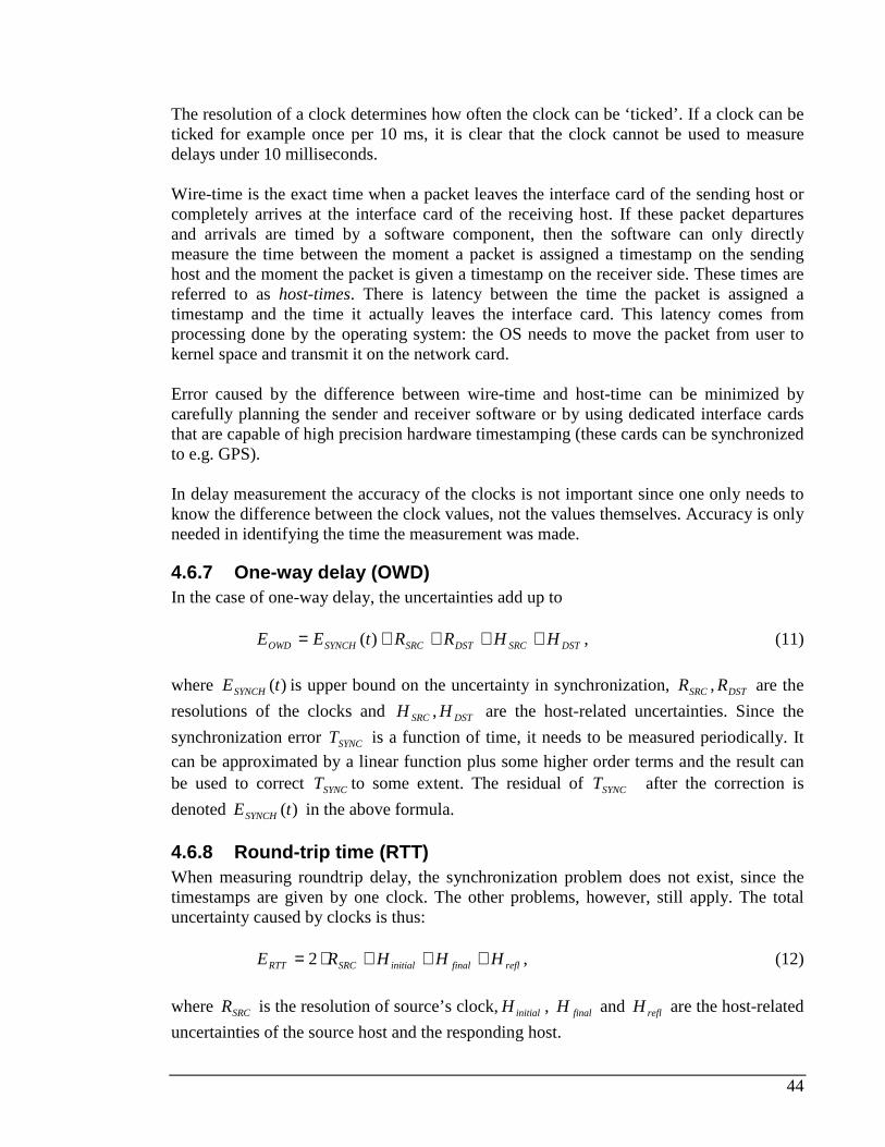
44

The resolution of a clock determines how often the clock can be ‘ticked’. If a clock can be ticked for example once per 10 ms, it is clear that the clock cannot be used to measure delays under 10 milliseconds. Wire-time is the exact time when a packet leaves the interface card of the sending host or completely arrives at the interface card of the receiving host. If these packet departures and arrivals are timed by a software component, then the software can only directly measure the time between the moment a packet is assigned a timestamp on the sending host and the moment the packet is given a timestamp on the receiver side. These times are referred to as host-times. There is latency between the time the packet is assigned a timestamp and the time it actually leaves the interface card. This latency comes from processing done by the operating system: the OS needs to move the packet from user to kernel space and transmit it on the network card. Error caused by the difference between wire-time and host-time can be minimized by carefully planning the sender and receiver software or by using dedicated interface cards that are capable of high precision hardware timestamping (these cards can be synchronized to e.g. GPS). In delay measurement the accuracy of the clocks is not important since one only needs to know the difference between the clock values, not the values themselves. Accuracy is only needed in identifying the time the measurement was made.

4.6.7 One-way delay (OWD) In the case of one-way delay, the uncertainties add up to

DSTSRCDSTSRCSYNCHOWD HHRRtEE ++++= )( , (11)

where )(tESYNCH is upper bound on the uncertainty in synchronization, DSTSRC RR , are the

resolutions of the clocks and DSTSRC HH , are the host-related uncertainties. Since the

synchronization error SYNCT is a function of time, it needs to be measured periodically. It

can be approximated by a linear function plus some higher order terms and the result can be used to correct SYNCT to some extent. The residual of SYNCT after the correction is

denoted )(tESYNCH in the above formula.

4.6.8 Round-trip time (RTT) When measuring roundtrip delay, the synchronization problem does not exist, since the timestamps are given by one clock. The other problems, however, still apply. The total uncertainty caused by clocks is thus:

reflfinalinitialSRCRTT HHHRE +++⋅= 2 , (12)

where SRCR is the resolution of source’s clock,initialH , finalH and reflH are the host-related

uncertainties of the source host and the responding host.

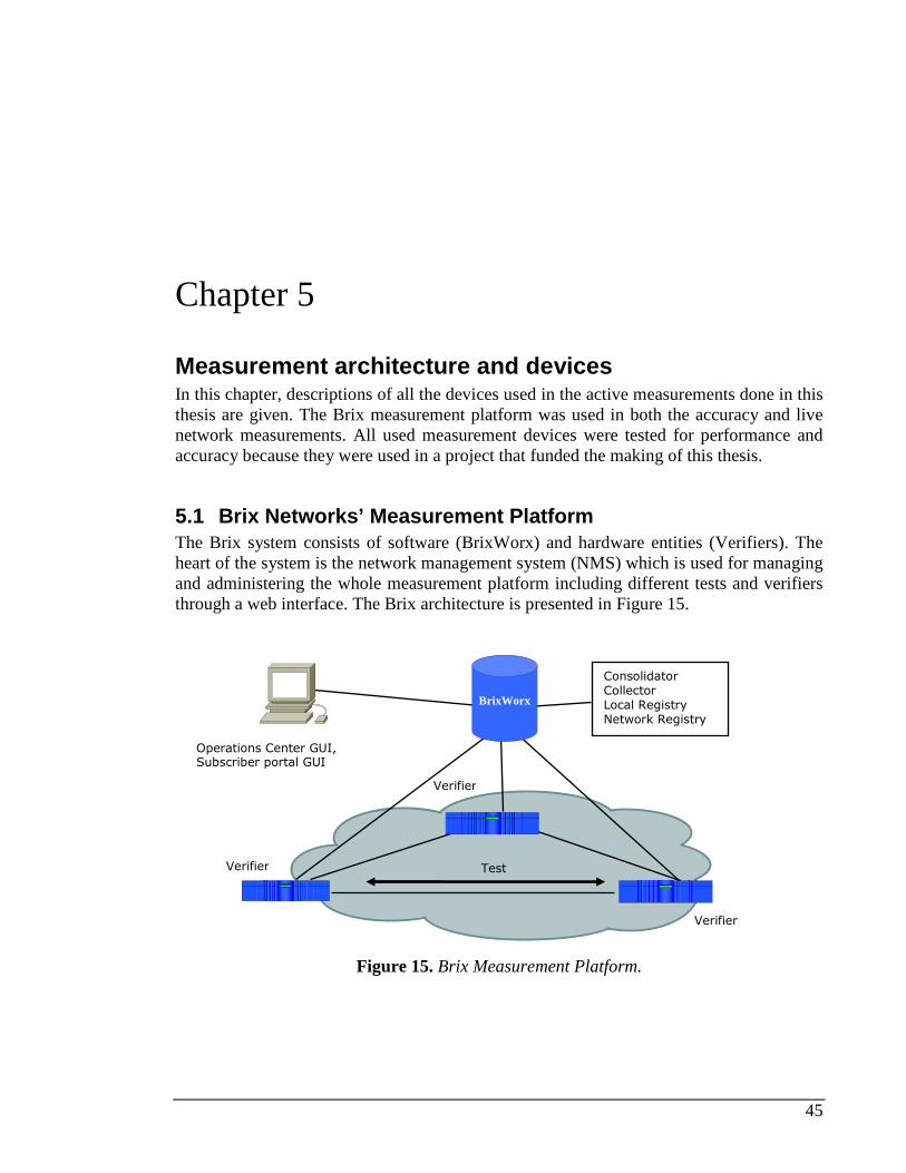
45

Chapter 5

Measurement architecture and devices In this chapter, descriptions of all the devices used in the active measurements done in this thesis are given. The Brix measurement platform was used in both the accuracy and live network measurements. All used measurement devices were tested for performance and accuracy because they were used in a project that funded the making of this thesis.

5.1 Brix Networks’ Measurement Platform The Brix system consists of software (BrixWorx) and hardware entities (Verifiers). The heart of the system is the network management system (NMS) which is used for managing and administering the whole measurement platform including different tests and verifiers through a web interface. The Brix architecture is presented in Figure 15.

Figure 15. Brix Measurement Platform.

Operations Center GUI, Subscriber portal GUI

Verifier

Verifier

Verifier

Consolidator Collector Local Registry Network Registry

Test

BrixWorx

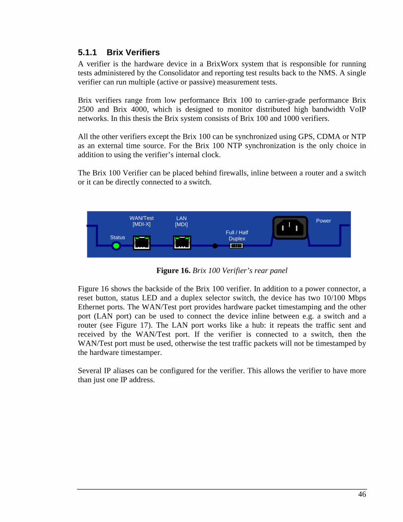
46

5.1.1 Brix Verifiers A verifier is the hardware device in a BrixWorx system that is responsible for running tests administered by the Consolidator and reporting test results back to the NMS. A single verifier can run multiple (active or passive) measurement tests. Brix verifiers range from low performance Brix 100 to carrier-grade performance Brix 2500 and Brix 4000, which is designed to monitor distributed high bandwidth VoIP networks. In this thesis the Brix system consists of Brix 100 and 1000 verifiers. All the other verifiers except the Brix 100 can be synchronized using GPS, CDMA or NTP as an external time source. For the Brix 100 NTP synchronization is the only choice in addition to using the verifier’s internal clock. The Brix 100 Verifier can be placed behind firewalls, inline between a router and a switch or it can be directly connected to a switch.

Figure 16. Brix 100 Verifier’s rear panel

Figure 16 shows the backside of the Brix 100 verifier. In addition to a power connector, a reset button, status LED and a duplex selector switch, the device has two 10/100 Mbps Ethernet ports. The WAN/Test port provides hardware packet timestamping and the other port (LAN port) can be used to connect the device inline between e.g. a switch and a router (see Figure 17). The LAN port works like a hub: it repeats the traffic sent and received by the WAN/Test port. If the verifier is connected to a switch, then the WAN/Test port must be used, otherwise the test traffic packets will not be timestamped by the hardware timestamper. Several IP aliases can be configured for the verifier. This allows the verifier to have more than just one IP address.

WAN/Test [MDI-X]

LAN [MDI]

Full / Half Duplex Status

Power

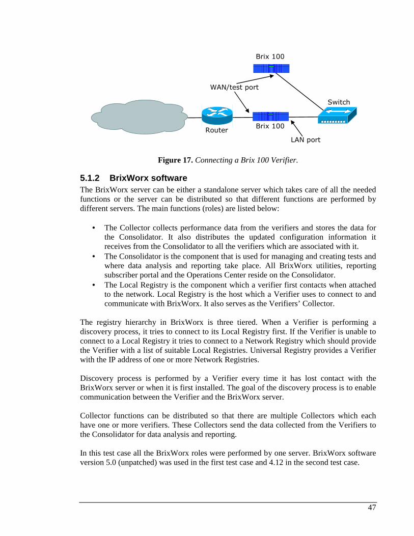
47

Figure 17. Connecting a Brix 100 Verifier.

5.1.2 BrixWorx software The BrixWorx server can be either a standalone server which takes care of all the needed functions or the server can be distributed so that different functions are performed by different servers. The main functions (roles) are listed below:

• The Collector collects performance data from the verifiers and stores the data for the Consolidator. It also distributes the updated configuration information it receives from the Consolidator to all the verifiers which are associated with it.

• The Consolidator is the component that is used for managing and creating tests and where data analysis and reporting take place. All BrixWorx utilities, reporting subscriber portal and the Operations Center reside on the Consolidator.

• The Local Registry is the component which a verifier first contacts when attached to the network. Local Registry is the host which a Verifier uses to connect to and communicate with BrixWorx. It also serves as the Verifiers’ Collector.

The registry hierarchy in BrixWorx is three tiered. When a Verifier is performing a discovery process, it tries to connect to its Local Registry first. If the Verifier is unable to connect to a Local Registry it tries to connect to a Network Registry which should provide the Verifier with a list of suitable Local Registries. Universal Registry provides a Verifier with the IP address of one or more Network Registries. Discovery process is performed by a Verifier every time it has lost contact with the BrixWorx server or when it is first installed. The goal of the discovery process is to enable communication between the Verifier and the BrixWorx server. Collector functions can be distributed so that there are multiple Collectors which each have one or more verifiers. These Collectors send the data collected from the Verifiers to the Consolidator for data analysis and reporting. In this test case all the BrixWorx roles were performed by one server. BrixWorx software version 5.0 (unpatched) was used in the first test case and 4.12 in the second test case.

Router Brix 100

Switch

Brix 100

WAN/test port

LAN port

48

5.1.3 Configuring Brix Verifiers Before the verifiers can be taken into use, they have to be properly configured so that they are able to connect to and communicate with the BrixWorx server. There are several ways to configure a verifier. Normally you make configuration changes to a verifier by using the BrixWorx Operation Center or by using the Command Line Interface (CLI) via a telnet connection, but this is only possible if the verifier is already able to communicate with the BrixWorx server. When a verifier arrives from the manufacturer, it generally is not able to communicate with the BrixWorx server since it first needs to have several network specific settings (e.g. IP address, server’s IP address etc.) changed. This configuration process can be either done manually (bench configuration) or automatically. If Dynamic Host Configuration Protocol (DHCP) or BOOTstrap Protocol (BOOTP) is used, the bench configuration process is not required: if a verifier has a connection to the Brix Universal Registry, it can download the correct settings from the registry. In situations where Internet connection is not available, thus there is no connection to the Universal Registry, all the required configurations have to be done manually.

5.1.4 Bench configuring When preparing a verifier to be shipped to a remote location, it is useful to bench configure the verifier. In bench configuring all the verifier’s basic settings are changed to match the current network environment and the changes are stored into the verifier’s flash memory. The bench configured settings become the default settings for the verifier so that whenever the verifier’s flash is cleared, the default settings become active. It must be noted that while bench configuring changes the verifier’s settings (semi)permanently, the other configuration methods will overwrite the bench configuration settings, but only until the verifier’s file system is cleared: the bench configured settings will become active and the other settings will be overwritten.

5.1.5 Bench configuring Brix 100 A special dongle is required when bench configuring Brix 100 verifiers locally. The dongle needs to be present in the WAN/Test port of the verifier. A PC with the following IP address:

192.168.168.n/24, where n = 1..167 or n = 169..254 can be used to connect to the LAN port of the verifier (Telnet session). The verifier’s default IP address is 192.168.168.168. To log in to the verifier for the first time, the default username (admin) and password (admin) must be used. When in the bench configuration mode (enter bench-cfg to change the mode) usually at least the following settings have to be set:

• Comm-Port number (BrixWorx server port) • Default gateway address • IP address, network mask and IP acquisition method • Domain

49

• DNS server address • Server discovery addresses (local, network and universal)

The new settings must be written to the flash before they can be taken into use. This is done by entering the end or the exit command to exit the bench configuration mode. When the basic settings have been stored to the verifier’s flash, the verifier’s file system has to be cleared by holding down the reset button for at least 5 seconds. After resetting, the bench configured settings become the default values for the verifier: whenever the verifier’s file system is cleared, the bench configured values are returned. Once the verifier is communicating with the BrixWorx server, all the other settings may be configured from the Operations Center. Also, the settings mentioned above can later be changed from the Operations Center.

5.1.6 Bench configuring Brix 1000 Configuring a Brix 1000 verifier is identical to configuring a Brix 100; the only difference is that the dongle is not required. A Brix 1000 includes a console port so all initial configuration can be done by using it. If further configuration changes are needed, they can be made via the operations center or by using the CLI via console or management ports (assuming that telnet or SSH management is allowed).

5.2 Echo-1 These devices are meant to be used as cheap and easy to install echo servers. Their main function is to echo back packets to a device sending (e.g. a Brix verifier) UDP Echo probes. This allows the measurement of round-trip delay and reachability. While Echo-1’s are not designed to be high performance they respond to echo packets with good precision (i.e. the round-trip time distribution is narrow in a fast, low latency network).

5.3 Juniper M7i JUNOS, the operating system used in Juniper’s routers, includes a Real-time Performance Monitor (RPM) feature that allows active measurements to be made with the router. RPM is covered in more detail in section 3.13.2.

5.4 Spirent AX4000 (Adtech) Spirent’s AX4000 broadband performance and QoS testing system is a traffic generator/analyzer capable of creating and analyzing traffic at speeds up to 10 Gbps depending on the configuration. In this thesis AX4000 is used in creating a steady stream of packets across a network to measure the one-way delay of the network.

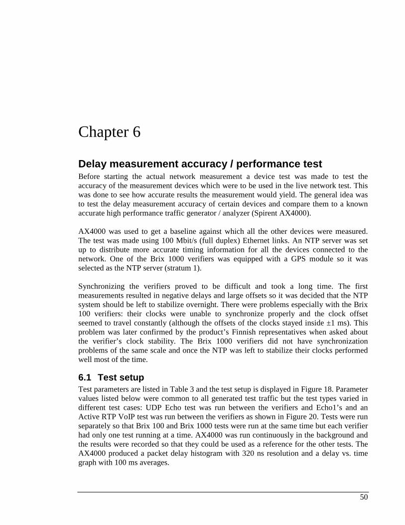
50

Chapter 6

Delay measurement accuracy / performance test Before starting the actual network measurement a device test was made to test the accuracy of the measurement devices which were to be used in the live network test. This was done to see how accurate results the measurement would yield. The general idea was to test the delay measurement accuracy of certain devices and compare them to a known accurate high performance traffic generator / analyzer (Spirent AX4000). AX4000 was used to get a baseline against which all the other devices were measured. The test was made using 100 Mbit/s (full duplex) Ethernet links. An NTP server was set up to distribute more accurate timing information for all the devices connected to the network. One of the Brix 1000 verifiers was equipped with a GPS module so it was selected as the NTP server (stratum 1). Synchronizing the verifiers proved to be difficult and took a long time. The first measurements resulted in negative delays and large offsets so it was decided that the NTP system should be left to stabilize overnight. There were problems especially with the Brix 100 verifiers: their clocks were unable to synchronize properly and the clock offset seemed to travel constantly (although the offsets of the clocks stayed inside ±1 ms). This problem was later confirmed by the product’s Finnish representatives when asked about the verifier’s clock stability. The Brix 1000 verifiers did not have synchronization problems of the same scale and once the NTP was left to stabilize their clocks performed well most of the time.

6.1 Test setup Test parameters are listed in Table 3 and the test setup is displayed in Figure 18. Parameter values listed below were common to all generated test traffic but the test types varied in different test cases: UDP Echo test was run between the verifiers and Echo1’s and an Active RTP VoIP test was run between the verifiers as shown in Figure 20. Tests were run separately so that Brix 100 and Brix 1000 tests were run at the same time but each verifier had only one test running at a time. AX4000 was run continuously in the background and the results were recorded so that they could be used as a reference for the other tests. The AX4000 produced a packet delay histogram with 320 ns resolution and a delay vs. time graph with 100 ms averages.

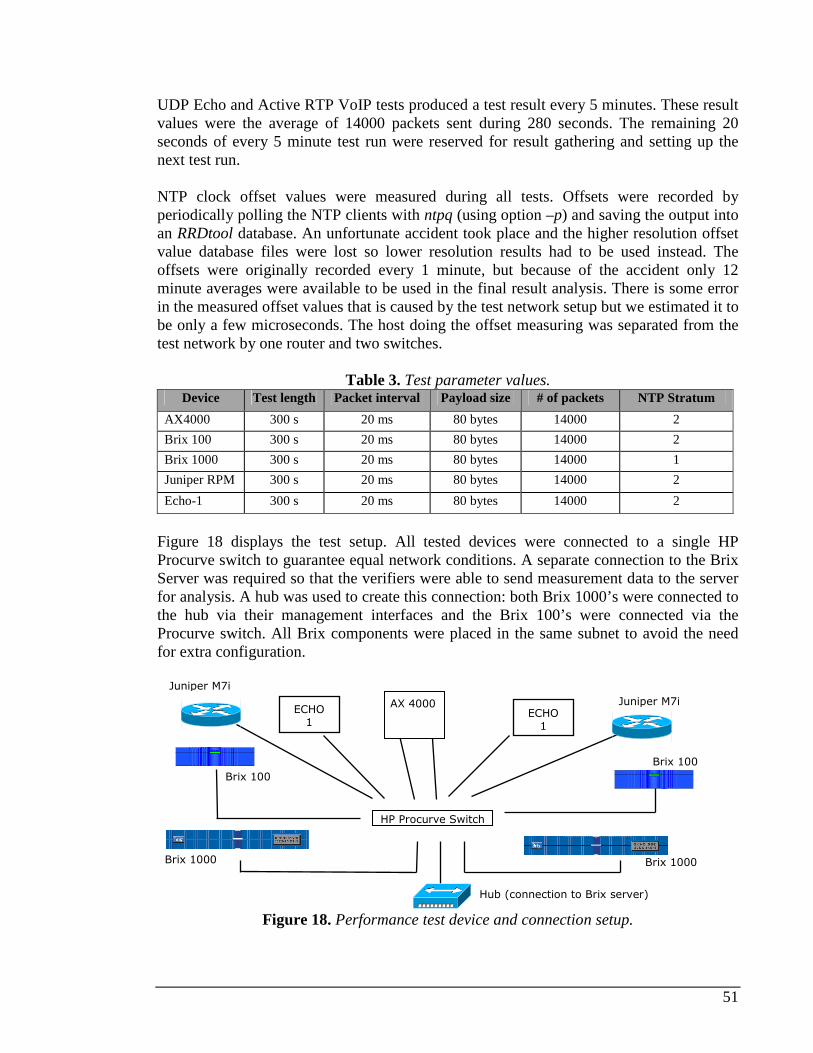
51

UDP Echo and Active RTP VoIP tests produced a test result every 5 minutes. These result values were the average of 14000 packets sent during 280 seconds. The remaining 20 seconds of every 5 minute test run were reserved for result gathering and setting up the next test run. NTP clock offset values were measured during all tests. Offsets were recorded by periodically polling the NTP clients with ntpq (using option –p) and saving the output into an RRDtool database. An unfortunate accident took place and the higher resolution offset value database files were lost so lower resolution results had to be used instead. The offsets were originally recorded every 1 minute, but because of the accident only 12 minute averages were available to be used in the final result analysis. There is some error in the measured offset values that is caused by the test network setup but we estimated it to be only a few microseconds. The host doing the offset measuring was separated from the test network by one router and two switches.

Table 3. Test parameter values. Device Test length Packet interval Payload size # of packets NTP Stratum

AX4000 300 s 20 ms 80 bytes 14000 2

Brix 100 300 s 20 ms 80 bytes 14000 2

Brix 1000 300 s 20 ms 80 bytes 14000 1

Juniper RPM 300 s 20 ms 80 bytes 14000 2

Echo-1 300 s 20 ms 80 bytes 14000 2

Figure 18 displays the test setup. All tested devices were connected to a single HP Procurve switch to guarantee equal network conditions. A separate connection to the Brix Server was required so that the verifiers were able to send measurement data to the server for analysis. A hub was used to create this connection: both Brix 1000’s were connected to the hub via their management interfaces and the Brix 100’s were connected via the Procurve switch. All Brix components were placed in the same subnet to avoid the need for extra configuration.

Figure 18. Performance test device and connection setup.

Brix 100

Brix 100

Brix 1000 Brix 1000

Juniper M7i

Juniper M7i

Hub (connection to Brix server)

ECHO 1

ECHO 1

AX 4000

HP Procurve Switch

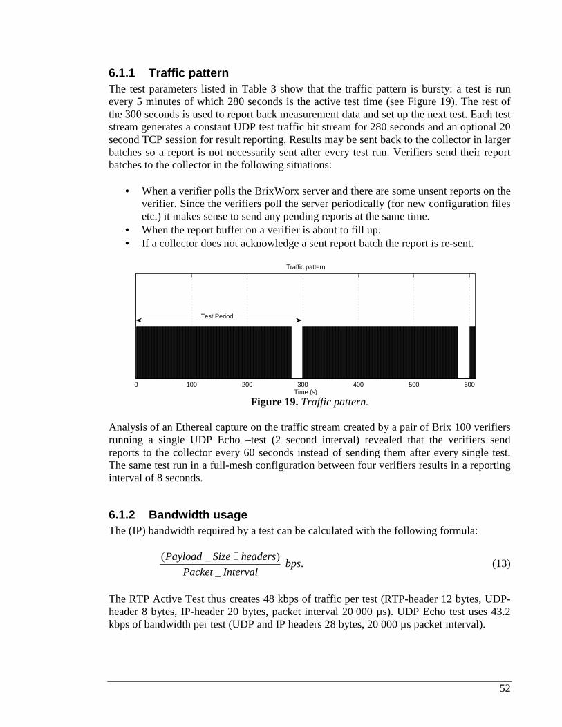
52

6.1.1 Traffic pattern The test parameters listed in Table 3 show that the traffic pattern is bursty: a test is run every 5 minutes of which 280 seconds is the active test time (see Figure 19). The rest of the 300 seconds is used to report back measurement data and set up the next test. Each test stream generates a constant UDP test traffic bit stream for 280 seconds and an optional 20 second TCP session for result reporting. Results may be sent back to the collector in larger batches so a report is not necessarily sent after every test run. Verifiers send their report batches to the collector in the following situations:

• When a verifier polls the BrixWorx server and there are some unsent reports on the verifier. Since the verifiers poll the server periodically (for new configuration files etc.) it makes sense to send any pending reports at the same time.

• When the report buffer on a verifier is about to fill up. • If a collector does not acknowledge a sent report batch the report is re-sent.

0 100 200 300 400 500 600

Traffic pattern

Time (s)

Test Period

Figure 19. Traffic pattern.

Analysis of an Ethereal capture on the traffic stream created by a pair of Brix 100 verifiers running a single UDP Echo –test (2 second interval) revealed that the verifiers send reports to the collector every 60 seconds instead of sending them after every single test. The same test run in a full-mesh configuration between four verifiers results in a reporting interval of 8 seconds.

6.1.2 Bandwidth usage The (IP) bandwidth required by a test can be calculated with the following formula:

IntervalPacket

headersSizePayload

_

)_( + bps. (13)

The RTP Active Test thus creates 48 kbps of traffic per test (RTP-header 12 bytes, UDP-header 8 bytes, IP-header 20 bytes, packet interval 20 000 µs). UDP Echo test uses 43.2 kbps of bandwidth per test (UDP and IP headers 28 bytes, 20 000 µs packet interval).

53

The result reports create only a negligible amount of traffic (in the area of 10 kB per minute). The size of a report batch depends on various factors including the verifier’s network connection type and the bandwidth allocated for testing and reporting.

6.2 Test results All tests produced a large amount of data and figures so therefore only the most significant figures are presented. Each test case’s results are summarized under their respective headings. Active RTP VoIP test produced one-way delay statistics while the UDP Echo test only produced round-trip time statistics. Figure 20 displays all different test cases that were run. Note that the results show negative delay values in some figures. While in reality there is no such thing as negative delay, measurement results may in some cases produce negative values. Often this is due to problems in synchronization as it was in this case: the clock of the receiving end was ahead of the clock at the sending end.

Figure 20. Different tests cases between devices.

6.2.1 Measured delay distribution Figure 21 summarizes the accuracy of the different devices. It displays the cumulative probability distribution of both Brix verifier types (with and without NTP correction) and the AX4000 used as a baseline for the measurement. In reality, the delay distribution measured with AX4000 represents the delay distribution created by the network switch (HP Procurve). The effect of Ethernet cables (6 meters in total) in the total delay is negligible.

Brix_100_2 Brix_100_1

Brix_1000_1 Brix_1000_2

Juniper_2 Juniper_1

ECHO 1_2

ECHO 1_1

Card 1

Card 2

Juniper RPM Ping

Active RTP VoIP test

Active RTP VoIP test

UDP Echo test

UDP Echo test Active RTP VoIP test

AX Test traffic

AX 4000

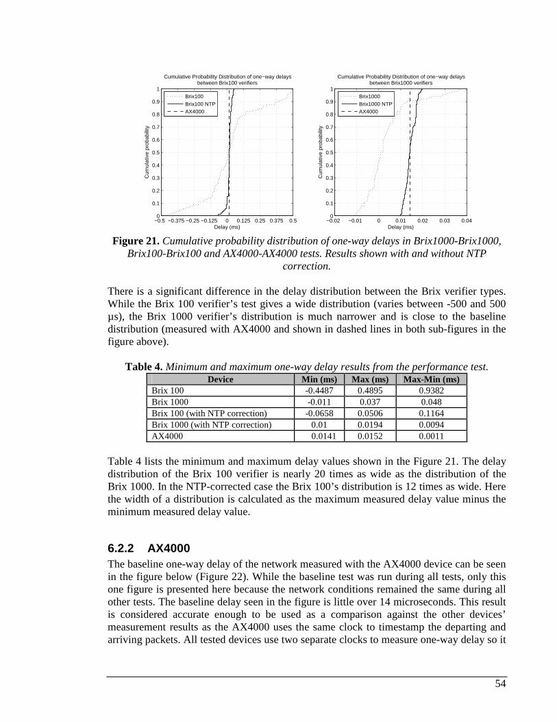
54

−0.5 −0.375 −0.25 −0.125 0 0.125 0.25 0.375 0.50

0.1

0.2

0.3

0.4

0.5

0.6

0.7

0.8

0.9

1

Cumulative Probability Distribution of one−way delaysbetween Brix100 verifiers

Delay (ms)

Cum

ulat

ive

prob

abili

ty

Brix100Brix100 NTPAX4000

−0.02 −0.01 0 0.01 0.02 0.03 0.040

0.1

0.2

0.3

0.4

0.5

0.6

0.7

0.8

0.9

1

Cumulative Probability Distribution of one−way delaysbetween Brix1000 verifiers

Delay (ms)

Cum

ulat

ive

prob

abili

ty

Brix1000Brix1000 NTPAX4000

Figure 21. Cumulative probability distribution of one-way delays in Brix1000-Brix1000,

Brix100-Brix100 and AX4000-AX4000 tests. Results shown with and without NTP correction.

There is a significant difference in the delay distribution between the Brix verifier types. While the Brix 100 verifier’s test gives a wide distribution (varies between -500 and 500 µs), the Brix 1000 verifier’s distribution is much narrower and is close to the baseline distribution (measured with AX4000 and shown in dashed lines in both sub-figures in the figure above).

Table 4. Minimum and maximum one-way delay results from the performance test. Device Min (ms) Max (ms) Max-Min (ms)

Brix 100 -0.4487 0.4895 0.9382 Brix 1000 -0.011 0.037 0.048 Brix 100 (with NTP correction) -0.0658 0.0506 0.1164 Brix 1000 (with NTP correction) 0.01 0.0194 0.0094 AX4000 0.0141 0.0152 0.0011

Table 4 lists the minimum and maximum delay values shown in the Figure 21. The delay distribution of the Brix 100 verifier is nearly 20 times as wide as the distribution of the Brix 1000. In the NTP-corrected case the Brix 100’s distribution is 12 times as wide. Here the width of a distribution is calculated as the maximum measured delay value minus the minimum measured delay value.

6.2.2 AX4000 The baseline one-way delay of the network measured with the AX4000 device can be seen in the figure below (Figure 22). While the baseline test was run during all tests, only this one figure is presented here because the network conditions remained the same during all other tests. The baseline delay seen in the figure is little over 14 microseconds. This result is considered accurate enough to be used as a comparison against the other devices’ measurement results as the AX4000 uses the same clock to timestamp the departing and arriving packets. All tested devices use two separate clocks to measure one-way delay so it

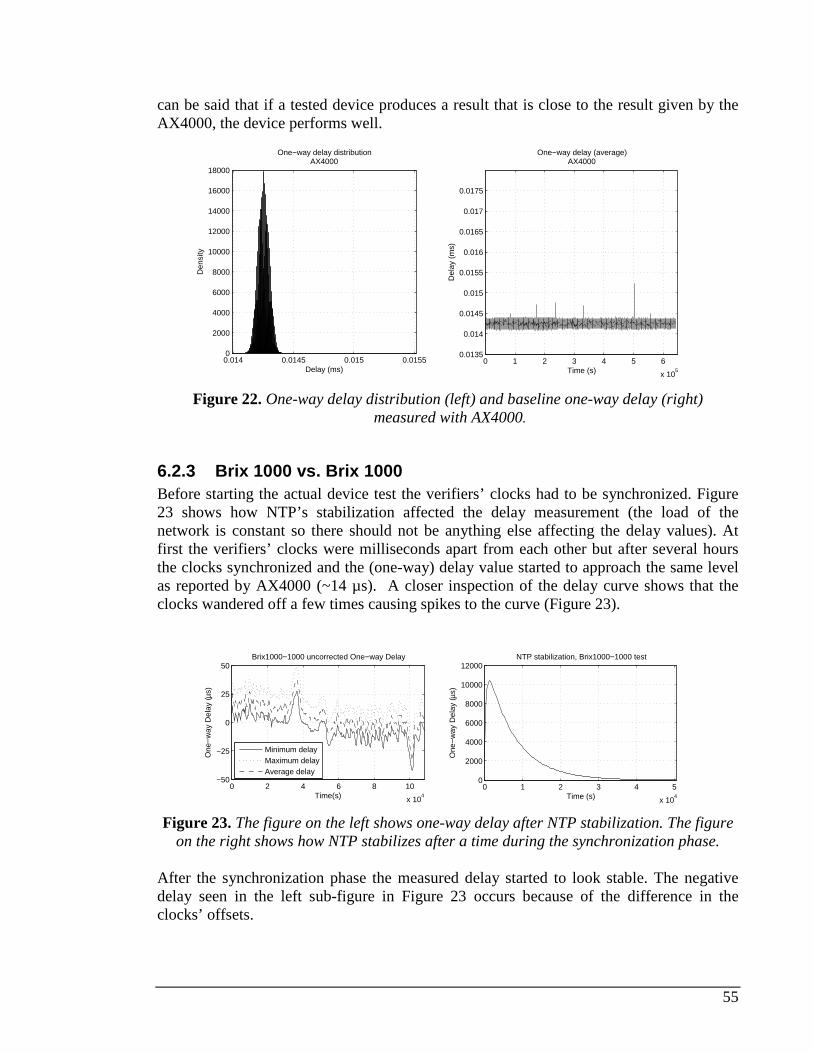
55

can be said that if a tested device produces a result that is close to the result given by the AX4000, the device performs well.

0.014 0.0145 0.015 0.01550

2000

4000

6000

8000

10000

12000

14000

16000

18000

Delay (ms)

Den

sity

One−way delay distributionAX4000

0 1 2 3 4 5 6

x 105

0.0135

0.014

0.0145

0.015

0.0155

0.016

0.0165

0.017

0.0175

One−way delay (average)AX4000

Time (s)

Del

ay (

ms)

Figure 22. One-way delay distribution (left) and baseline one-way delay (right)

measured with AX4000.

6.2.3 Brix 1000 vs. Brix 1000 Before starting the actual device test the verifiers’ clocks had to be synchronized. Figure 23 shows how NTP’s stabilization affected the delay measurement (the load of the network is constant so there should not be anything else affecting the delay values). At first the verifiers’ clocks were milliseconds apart from each other but after several hours the clocks synchronized and the (one-way) delay value started to approach the same level as reported by AX4000 (~14 µs). A closer inspection of the delay curve shows that the clocks wandered off a few times causing spikes to the curve (Figure 23).

0 2 4 6 8 10

x 104

−50

−25

0

25

50Brix1000−1000 uncorrected One−way Delay

Time(s)

One

−w

ay D

elay

(µs)

0 1 2 3 4 5

x 104

0

2000

4000

6000

8000

10000

12000NTP stabilization, Brix1000−1000 test

Time (s)

One

−w

ay D

elay

(µs)

Minimum delayMaximum delayAverage delay

Figure 23. The figure on the left shows one-way delay after NTP stabilization. The figure

on the right shows how NTP stabilizes after a time during the synchronization phase. After the synchronization phase the measured delay started to look stable. The negative delay seen in the left sub-figure in Figure 23 occurs because of the difference in the clocks’ offsets.

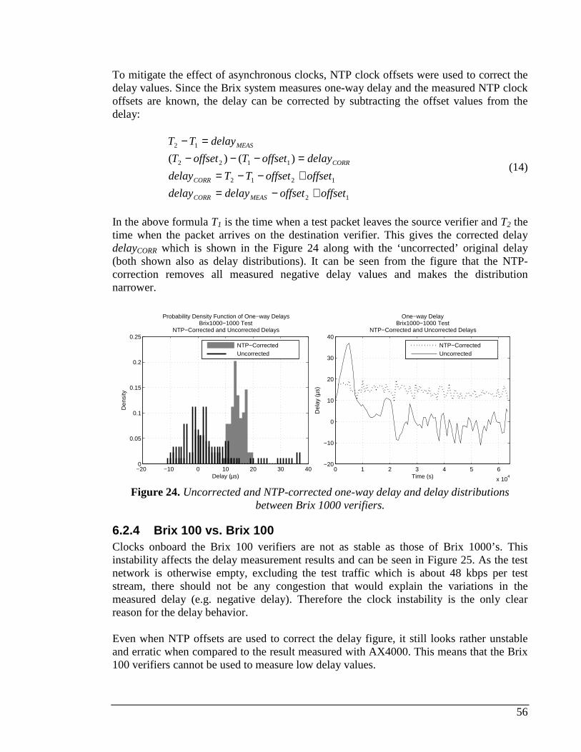
56

To mitigate the effect of asynchronous clocks, NTP clock offsets were used to correct the delay values. Since the Brix system measures one-way delay and the measured NTP clock offsets are known, the delay can be corrected by subtracting the offset values from the delay:

12

1212

1122

12

)()(

offsetoffsetdelaydelay

offsetoffsetTTdelay

delayoffsetToffsetT

delayTT

MEASCORR

CORR

CORR

MEAS

+−=+−−==−−−

=−

(14)

In the above formula T1 is the time when a test packet leaves the source verifier and T2 the time when the packet arrives on the destination verifier. This gives the corrected delay delayCORR which is shown in the Figure 24 along with the ‘uncorrected’ original delay (both shown also as delay distributions). It can be seen from the figure that the NTP-correction removes all measured negative delay values and makes the distribution narrower.

−20 −10 0 10 20 30 400

0.05

0.1

0.15

0.2

0.25

Delay (µs)

Den

sity

Probability Density Function of One−way DelaysBrix1000−1000 Test

NTP−Corrected and Uncorrected Delays

0 1 2 3 4 5 6

x 104

−20

−10

0

10

20

30

40

One−way DelayBrix1000−1000 Test

NTP−Corrected and Uncorrected Delays

Time (s)

Del

ay (µ

s)

NTP−CorrectedUncorrected

NTP−CorrectedUncorrected

Figure 24. Uncorrected and NTP-corrected one-way delay and delay distributions

between Brix 1000 verifiers.

6.2.4 Brix 100 vs. Brix 100 Clocks onboard the Brix 100 verifiers are not as stable as those of Brix 1000’s. This instability affects the delay measurement results and can be seen in Figure 25. As the test network is otherwise empty, excluding the test traffic which is about 48 kbps per test stream, there should not be any congestion that would explain the variations in the measured delay (e.g. negative delay). Therefore the clock instability is the only clear reason for the delay behavior. Even when NTP offsets are used to correct the delay figure, it still looks rather unstable and erratic when compared to the result measured with AX4000. This means that the Brix 100 verifiers cannot be used to measure low delay values.

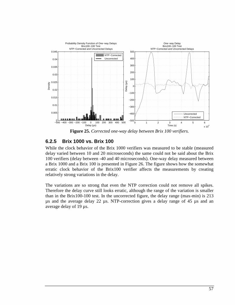
57

−500 −400 −300 −200 −100 0 100 200 300 400 5000

0.005

0.01

0.015

0.02

0.025

0.03

0.035

0.04

0.045

Delay (µs)

Den

sity

Probability Density Function of One−way DelaysBrix100−100 Test

NTP−Corrected and Uncorrected Delays

0 1 2 3 4 5 6

x 104

−500

−400

−300

−200

−100

0

100

200

300

400

500

One−way DelayBrix100−100 Test

NTP−Corrected and Uncorrected Delays

Time (s)D

elay

(µs)

NTP−CorrectedUncorrected

UncorrectedNTP−Corrected

Figure 25. Corrected one-way delay between Brix 100 verifiers.

6.2.5 Brix 1000 vs. Brix 100 While the clock behavior of the Brix 1000 verifiers was measured to be stable (measured delay varied between 10 and 20 microseconds) the same could not be said about the Brix 100 verifiers (delay between -40 and 40 microseconds). One-way delay measured between a Brix 1000 and a Brix 100 is presented in Figure 26. The figure shows how the somewhat erratic clock behavior of the Brix100 verifier affects the measurements by creating relatively strong variations in the delay. The variations are so strong that even the NTP correction could not remove all spikes. Therefore the delay curve still looks erratic, although the range of the variation is smaller than in the Brix100-100 test. In the uncorrected figure, the delay range (max-min) is 213 µs and the average delay 22 µs. NTP-correction gives a delay range of 45 µs and an average delay of 19 µs.

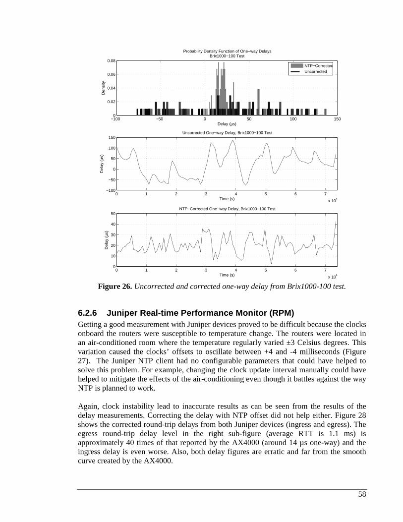
58

−100 −50 0 50 100 1500

0.02

0.04

0.06

0.08

Delay (µs)

Den

sity

Probability Density Function of One−way DelaysBrix1000−100 Test

NTP−CorrectedUncorrected

0 1 2 3 4 5 6 7

x 104

−100

−50

0

50

100

150Uncorrected One−way Delay, Brix1000−100 Test

Time (s)

Del

ay (µ

s)

0 1 2 3 4 5 6 7

x 104

0

10

20

30

40

50NTP−Corrected One−way Delay, Brix1000−100 Test

Time (s)

Del

ay (µ

s)

Figure 26. Uncorrected and corrected one-way delay from Brix1000-100 test.

6.2.6 Juniper Real-time Performance Monitor (RPM) Getting a good measurement with Juniper devices proved to be difficult because the clocks onboard the routers were susceptible to temperature change. The routers were located in an air-conditioned room where the temperature regularly varied ±3 Celsius degrees. This variation caused the clocks’ offsets to oscillate between +4 and -4 milliseconds (Figure 27). The Juniper NTP client had no configurable parameters that could have helped to solve this problem. For example, changing the clock update interval manually could have helped to mitigate the effects of the air-conditioning even though it battles against the way NTP is planned to work. Again, clock instability lead to inaccurate results as can be seen from the results of the delay measurements. Correcting the delay with NTP offset did not help either. Figure 28 shows the corrected round-trip delays from both Juniper devices (ingress and egress). The egress round-trip delay level in the right sub-figure (average RTT is 1.1 ms) is approximately 40 times of that reported by the AX4000 (around 14 µs one-way) and the ingress delay is even worse. Also, both delay figures are erratic and far from the smooth curve created by the AX4000.

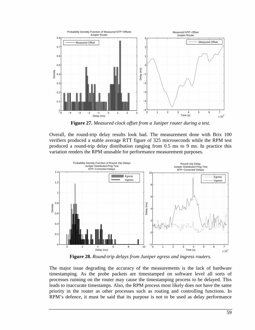
59

−5 −4 −3 −2 −1 0 1 2 30

0.1

0.2

0.3

0.4

0.5

0.6

0.7

0.8

Delay (ms)

Den

sity

Probability Denstity Function of Measured NTP−OffsetsJuniper Router

0 1 2 3 4 5 6 7

x 104

−5

−4

−3

−2

−1

0

1

2

3

Measured NTP−OffsetJuniper Router

Time (s)

Del

ay (

ms)

Measured Offset Measured Offset

Figure 27. Measured clock offset from a Juniper router during a test.

Overall, the round-trip delay results look bad. The measurement done with Brix 100 verifiers produced a stable average RTT figure of 325 microseconds while the RPM test produced a round-trip delay distribution ranging from 0.5 ms to 9 ms. In practice this variation renders the RPM unusable for performance measurement purposes.

0 2 4 6 8 100

0.2

0.4

0.6

0.8

1

1.2

1.4

Delay (ms)

Den

sity

Probability Density Function of Round−trip DelaysJuniper Distributed Ping Test

NTP−Corrected Delays

0 1 2 3 4 5 6 7

x 104

−2

0

2

4

6

8

10

Round−trip DelayJuniper Distributed Ping Test

NTP−Corrected Delays

Time (s)

Del

ay (

ms)

EgressIngress

EgressIngress

Figure 28. Round-trip delays from Juniper egress and ingress routers.

The major issue degrading the accuracy of the measurements is the lack of hardware timestamping. As the probe packets are timestamped on software level all sorts of processes running on the router may cause the timestamping process to be delayed. This leads to inaccurate timestamps. Also, the RPM process most likely does not have the same priority in the router as other processes such as routing and controlling functions. In RPM’s defence, it must be said that its purpose is not to be used as delay performance

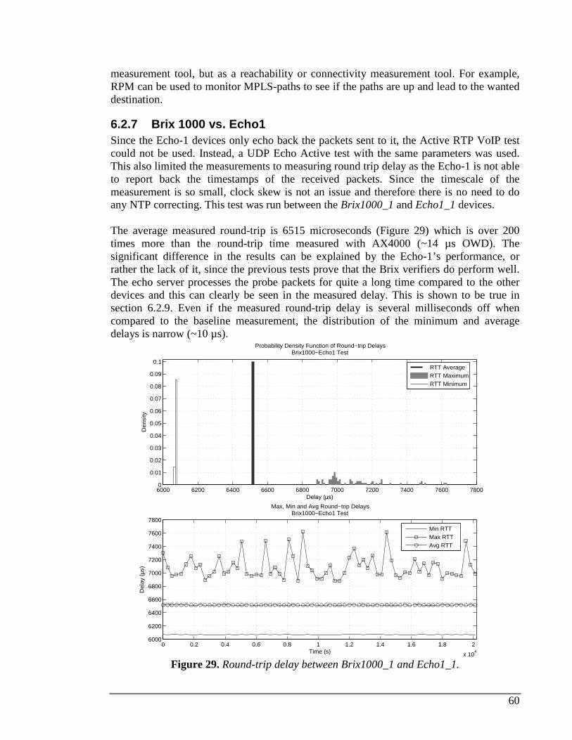
60

measurement tool, but as a reachability or connectivity measurement tool. For example, RPM can be used to monitor MPLS-paths to see if the paths are up and lead to the wanted destination.

6.2.7 Brix 1000 vs. Echo1 Since the Echo-1 devices only echo back the packets sent to it, the Active RTP VoIP test could not be used. Instead, a UDP Echo Active test with the same parameters was used. This also limited the measurements to measuring round trip delay as the Echo-1 is not able to report back the timestamps of the received packets. Since the timescale of the measurement is so small, clock skew is not an issue and therefore there is no need to do any NTP correcting. This test was run between the Brix1000_1 and Echo1_1 devices. The average measured round-trip is 6515 microseconds (Figure 29) which is over 200 times more than the round-trip time measured with AX4000 (~14 µs OWD). The significant difference in the results can be explained by the Echo-1’s performance, or rather the lack of it, since the previous tests prove that the Brix verifiers do perform well. The echo server processes the probe packets for quite a long time compared to the other devices and this can clearly be seen in the measured delay. This is shown to be true in section 6.2.9. Even if the measured round-trip delay is several milliseconds off when compared to the baseline measurement, the distribution of the minimum and average delays is narrow (~10 µs).

6000 6200 6400 6600 6800 7000 7200 7400 7600 78000

0.01

0.02

0.03

0.04

0.05

0.06

0.07

0.08

0.09

0.1

Delay (µs)

Den

sity

Probability Density Function of Round−trip DelaysBrix1000−Echo1 Test

RTT AverageRTT MaximumRTT Minimum

0 0.2 0.4 0.6 0.8 1 1.2 1.4 1.6 1.8 2

x 104

6000

6200

6400

6600

6800

7000

7200

7400

7600

7800

Max, Min and Avg Round−trip DelaysBrix1000−Echo1 Test

Time (s)

Del

ay (µ

s)

Min RTTMax RTTAvg RTT

Figure 29. Round-trip delay between Brix1000_1 and Echo1_1.

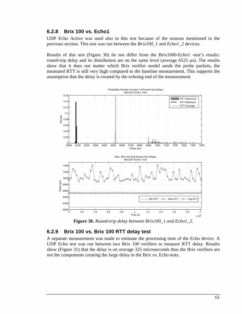
61

6.2.8 Brix 100 vs. Echo1 UDP Echo Active was used also in this test because of the reasons mentioned in the previous section. This test was run between the Brix100_1 and Echo1_2 devices. Results of this test (Figure 30) do not differ from the Brix1000-Echo1 -test’s results: round-trip delay and its distribution are on the same level (average 6525 µs). The results show that it does not matter which Brix verifier model sends the probe packets, the measured RTT is still very high compared to the baseline measurement. This supports the assumption that the delay is created by the echoing end of the measurement.

6000 6100 6200 6300 6400 6500 6600 6700 6800 6900 7000 7100 7200 7300 7400 75000

0.02

0.04

0.06

0.08

0.1

0.12

0.14

0.16

Delay (µs)

Den

sity

Probability Density Function of Round−trip DelaysBrix100−Echo1 Test

0 0.2 0.4 0.6 0.8 1 1.2 1.4 1.6 1.8 2

x 104

6000

6200

6400

6600

6800

7000

7200

7400

Max, Min and Avg Round−trip DelaysBrix100−Echo1 Test

Time (s)

Del

ay (µ

s)

Min RTT Max RTT Avg RTT

RTT MaximumRTT MinimumRTT Average

Figure 30. Round-trip delay between Brix100_1 and Echo1_2.

6.2.9 Brix 100 vs. Brix 100 RTT delay test A separate measurement was made to estimate the processing time of the Echo device. A UDP Echo test was run between two Brix 100 verifiers to measure RTT delay. Results show (Figure 31) that the delay is on average 325 microseconds thus the Brix verifiers are not the components creating the large delay in the Brix vs. Echo tests.

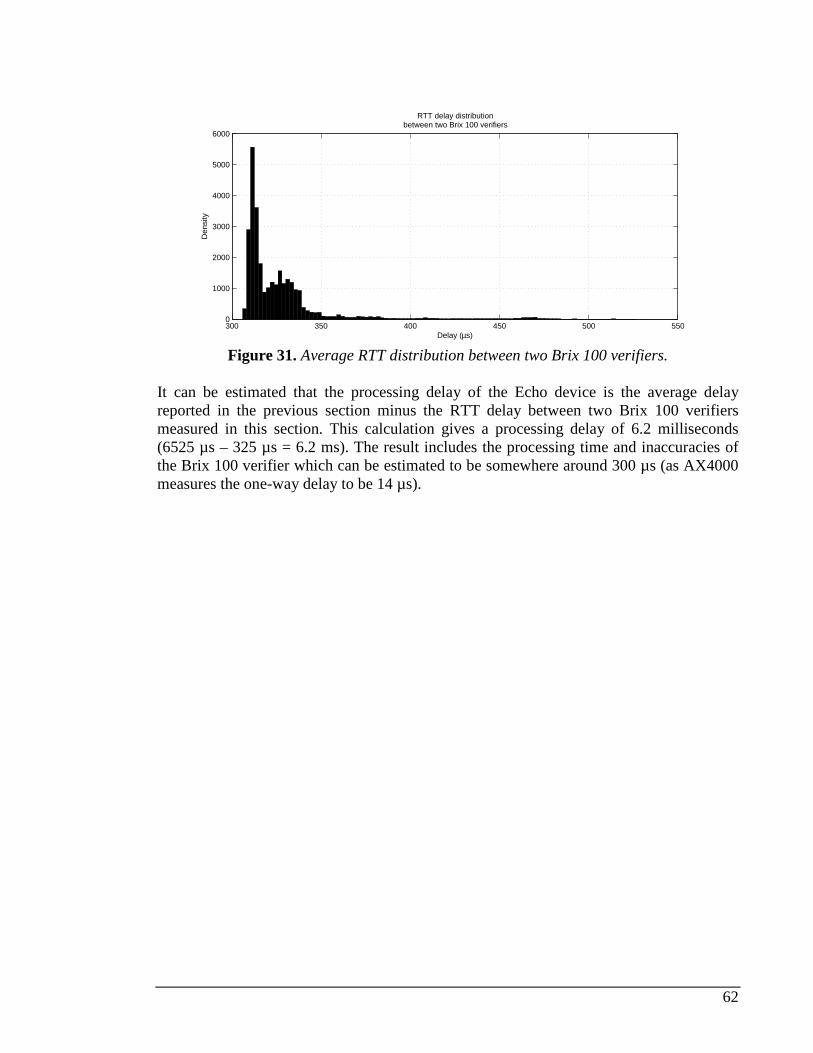
62

300 350 400 450 500 5500

1000

2000

3000

4000

5000

6000

Delay (µs)

Den

sity

RTT delay distributionbetween two Brix 100 verifiers

Figure 31. Average RTT distribution between two Brix 100 verifiers.

It can be estimated that the processing delay of the Echo device is the average delay reported in the previous section minus the RTT delay between two Brix 100 verifiers measured in this section. This calculation gives a processing delay of 6.2 milliseconds (6525 µs – 325 µs = 6.2 ms). The result includes the processing time and inaccuracies of the Brix 100 verifier which can be estimated to be somewhere around 300 µs (as AX4000 measures the one-way delay to be 14 µs).

63

Chapter 7

Measurements in a live network A series of live network tests were performed to test the Brix system’s capability to detect certain events in a network. These events include network breaks and network overload scenarios. Several Brix 100 verifiers were placed in selected locations in the network and a full mesh UDP Echo test was set up between them to record round-trip delay and packet loss.

7.1 Test network setup In this section the test device setup and configuration are explained. Also, technological and configurative choices are justified and discussed. The test network consisted of Juniper Networks’ M320 core and M10 access routers. Measurements were taken by using Brix Networks’ Brix System. A background load for the network was created by using Spirent’s SmartBits, AX4000 and NLANR’s IPerf software [79]. All sites were connected with MPLS VPNs and the label paths were protected by RSVP-TE backup tunnels (300 ms recovery time).

7.1.1 Network topology The network topology and verifier placement is shown in the figure below (Figure 32). In the actual network there were more sites than present in the figure, but due to lack of resources only the sites that were considered important were taken into the measurement. Also, the Brix 1000’s used in the performance test were not available in the live network measurement.

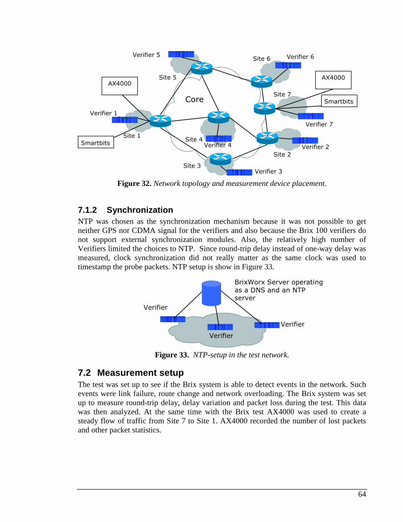
64

Figure 32. Network topology and measurement device placement.

7.1.2 Synchronization NTP was chosen as the synchronization mechanism because it was not possible to get neither GPS nor CDMA signal for the verifiers and also because the Brix 100 verifiers do not support external synchronization modules. Also, the relatively high number of Verifiers limited the choices to NTP. Since round-trip delay instead of one-way delay was measured, clock synchronization did not really matter as the same clock was used to timestamp the probe packets. NTP setup is show in Figure 33.

Figure 33. NTP-setup in the test network.

7.2 Measurement setup The test was set up to see if the Brix system is able to detect events in the network. Such events were link failure, route change and network overloading. The Brix system was set up to measure round-trip delay, delay variation and packet loss during the test. This data was then analyzed. At the same time with the Brix test AX4000 was used to create a steady flow of traffic from Site 7 to Site 1. AX4000 recorded the number of lost packets and other packet statistics.

BrixWorx Server operating

as a DNS and an NTP server

Verifier

Verifier

Verifier

Verifier 5

Core

Site 1 Site 4

Site 3

Site 2

Site 5

Site 6

Verifier 1

Verifier 6

Verifier 4

Verifier 3

Verifier 2

Verifier 7

Site 7

AX4000

AX4000

Smartbits

Smartbits

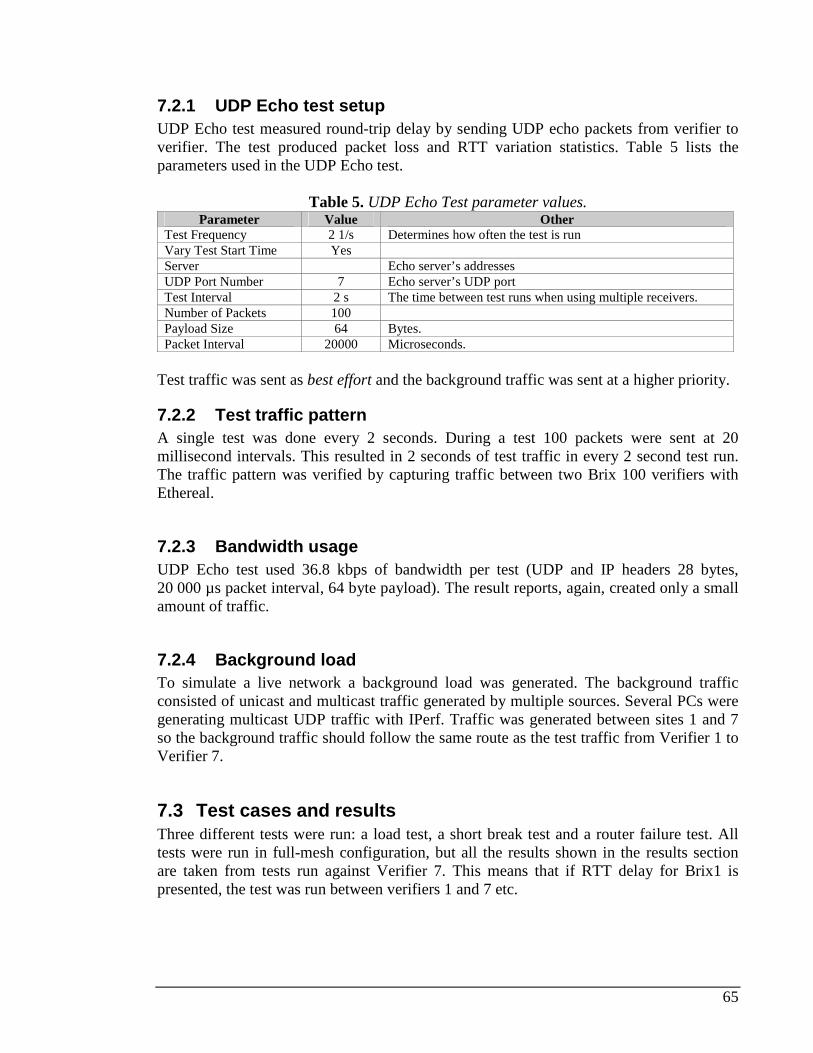
65

7.2.1 UDP Echo test setup UDP Echo test measured round-trip delay by sending UDP echo packets from verifier to verifier. The test produced packet loss and RTT variation statistics. Table 5 lists the parameters used in the UDP Echo test.

Table 5. UDP Echo Test parameter values. Parameter Value Other

Test Frequency 2 1/s Determines how often the test is run Vary Test Start Time Yes Server Echo server’s addresses UDP Port Number 7 Echo server’s UDP port Test Interval 2 s The time between test runs when using multiple receivers. Number of Packets 100 Payload Size 64 Bytes. Packet Interval 20000 Microseconds.

Test traffic was sent as best effort and the background traffic was sent at a higher priority.

7.2.2 Test traffic pattern A single test was done every 2 seconds. During a test 100 packets were sent at 20 millisecond intervals. This resulted in 2 seconds of test traffic in every 2 second test run. The traffic pattern was verified by capturing traffic between two Brix 100 verifiers with Ethereal.

7.2.3 Bandwidth usage UDP Echo test used 36.8 kbps of bandwidth per test (UDP and IP headers 28 bytes, 20 000 µs packet interval, 64 byte payload). The result reports, again, created only a small amount of traffic.

7.2.4 Background load To simulate a live network a background load was generated. The background traffic consisted of unicast and multicast traffic generated by multiple sources. Several PCs were generating multicast UDP traffic with IPerf. Traffic was generated between sites 1 and 7 so the background traffic should follow the same route as the test traffic from Verifier 1 to Verifier 7.

7.3 Test cases and results Three different tests were run: a load test, a short break test and a router failure test. All tests were run in full-mesh configuration, but all the results shown in the results section are taken from tests run against Verifier 7. This means that if RTT delay for Brix1 is presented, the test was run between verifiers 1 and 7 etc.

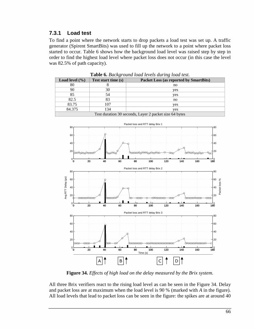
66

7.3.1 Load test To find a point where the network starts to drop packets a load test was set up. A traffic generator (Spirent SmartBits) was used to fill up the network to a point where packet loss started to occur. Table 6 shows how the background load level was raised step by step in order to find the highest load level where packet loss does not occur (in this case the level was 82.5% of path capacity).

Table 6. Background load levels during load test. Load level (%) Test start time (s) Packet Loss (as reported by SmartBits)

80 8 no 90 30 yes 85 54 yes

82.5 83 no 83.75 107 yes 84.375 134 yes

Test duration 30 seconds, Layer 2 packet size 64 bytes

0 20 40 60 80 100 120 140 160 1800

20

40

60

80Packet loss and RTT delay Brix 1

0 20 40 60 80 100 120 140 160 1800

20

40

60

80

0 20 40 60 80 100 120 140 160 1800

20

40

60

80

Avg

RT

T D

elay

(µs)

0 20 40 60 80 100 120 140 160 1800

20

40

60

80

Pac

ket l

oss

%

Packet loss and RTT delay Brix 2

0 20 40 60 80 100 120 140 160 1800

20

40

60

80

Time (s)0 20 40 60 80 100 120 140 160 180

0

20

40

60

80Packet loss and RTT delay Brix 3

Figure 34. Effects of high load on the delay measured by the Brix system.

All three Brix verifiers react to the rising load level as can be seen in the Figure 34. Delay and packet loss are at maximum when the load level is 90 % (marked with A in the figure). All load levels that lead to packet loss can be seen in the figure: the spikes are at around 40

A B C D

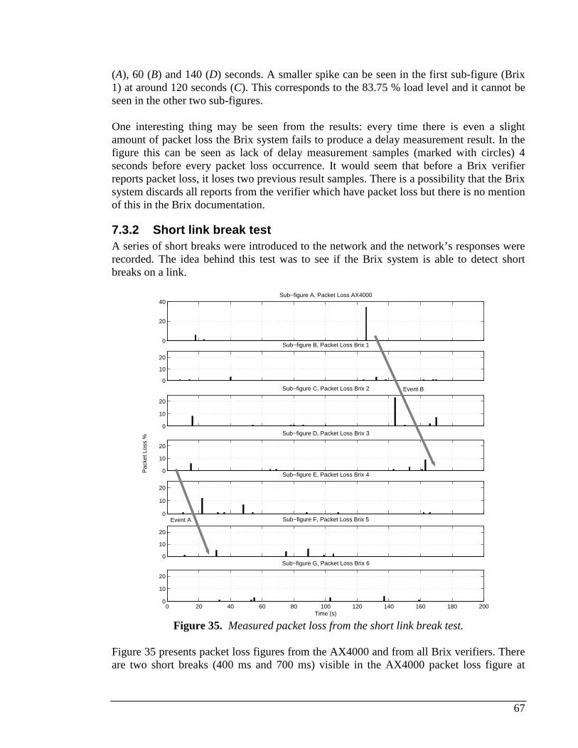
67

(A), 60 (B) and 140 (D) seconds. A smaller spike can be seen in the first sub-figure (Brix 1) at around 120 seconds (C). This corresponds to the 83.75 % load level and it cannot be seen in the other two sub-figures. One interesting thing may be seen from the results: every time there is even a slight amount of packet loss the Brix system fails to produce a delay measurement result. In the figure this can be seen as lack of delay measurement samples (marked with circles) 4 seconds before every packet loss occurrence. It would seem that before a Brix verifier reports packet loss, it loses two previous result samples. There is a possibility that the Brix system discards all reports from the verifier which have packet loss but there is no mention of this in the Brix documentation.

7.3.2 Short link break test A series of short breaks were introduced to the network and the network’s responses were recorded. The idea behind this test was to see if the Brix system is able to detect short breaks on a link.

0

20

40Sub−figure A, Packet Loss AX4000

0

10

20

Sub−figure B, Packet Loss Brix 1

0

10

20

Sub−figure C, Packet Loss Brix 2

0

10

20

Sub−figure D, Packet Loss Brix 3

0

10

20

Sub−figure E, Packet Loss Brix 4

0

10

20

Sub−figure F, Packet Loss Brix 5

0 20 40 60 80 100 120 140 160 180 2000

10

20

Sub−figure G, Packet Loss Brix 6

Time (s)

Pac

ket L

oss

%

Event B

Event A

Figure 35. Measured packet loss from the short link break test.

Figure 35 presents packet loss figures from the AX4000 and from all Brix verifiers. There are two short breaks (400 ms and 700 ms) visible in the AX4000 packet loss figure at

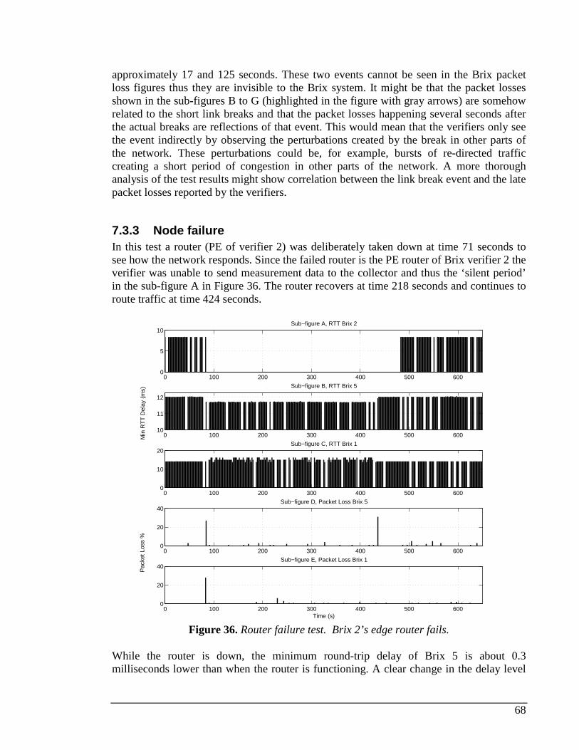
68

approximately 17 and 125 seconds. These two events cannot be seen in the Brix packet loss figures thus they are invisible to the Brix system. It might be that the packet losses shown in the sub-figures B to G (highlighted in the figure with gray arrows) are somehow related to the short link breaks and that the packet losses happening several seconds after the actual breaks are reflections of that event. This would mean that the verifiers only see the event indirectly by observing the perturbations created by the break in other parts of the network. These perturbations could be, for example, bursts of re-directed traffic creating a short period of congestion in other parts of the network. A more thorough analysis of the test results might show correlation between the link break event and the late packet losses reported by the verifiers.

7.3.3 Node failure In this test a router (PE of verifier 2) was deliberately taken down at time 71 seconds to see how the network responds. Since the failed router is the PE router of Brix verifier 2 the verifier was unable to send measurement data to the collector and thus the ‘silent period’ in the sub-figure A in Figure 36. The router recovers at time 218 seconds and continues to route traffic at time 424 seconds.

0 100 200 300 400 500 6000

20

40Sub−figure E, Packet Loss Brix 1

Time (s)

Pac

ket L

oss

%

0 100 200 300 400 500 6000

5

10Sub−figure A, RTT Brix 2

Min

RT

T D

elay

(m

s)

0 100 200 300 400 500 60010

11

12

Sub−figure B, RTT Brix 5

0 100 200 300 400 500 6000

10

20Sub−figure C, RTT Brix 1

0 100 200 300 400 500 6000

20

40Sub−figure D, Packet Loss Brix 5

Figure 36. Router failure test. Brix 2’s edge router fails.

While the router is down, the minimum round-trip delay of Brix 5 is about 0.3 milliseconds lower than when the router is functioning. A clear change in the delay level

69

can be seen in sub-figure B during the router’s downtime. This often results from a route change which is not so obvious in this case. It may be that there was a change in the routing once the router failed, but the notch in the delay level might also result from more network resources being available for the test traffic. When the router goes down, so does the high priority background traffic which means that the best effort test traffic gets more resources. This in turn might lead to lower delay especially if the network was highly loaded with high priority traffic. Sub-figure E shows that there is packet loss at the moment the router goes down. Probe packets were sent every 20 ms and 27 packets were lost after the failure. The network break can be calculated to have lasted approximately 0.54 seconds. Unfortunately the Brix system was not able to report any data back to the collector for 7 seconds after the node failure. This means that 3 to 4 test result reports are missing so the network break could have been a lot longer than the half a second Brix system reports. Missing test results can be seen in the Figure 36 as white spaces. The most notable missing test result set is the one seen in the Brix 2 RTT sub-figure where there is a gap of 400 seconds. There seems to be a lot of these gaps in the figures which just shows that the verifiers were not able to perform well enough during the test. This can be verified by the fact that these gaps appear even when there is no notable cross-traffic in the network and other measurement methods do not report packet loss (the reports are sent to the collector using TCP so packet loss should not affect it). Somehow the test results sent by the verifiers do not make it to the database and are lost somewhere during the way. From the round-trip delay sub-figure of Brix 5 it can be seen that the router fails after 77 seconds and recovers after 428 seconds. It is difficult to get the exact time of the events from the figures because the Brix system fails to record the measurement results from the moments when the failure and recovery occur. In addition, the two second resolution of the tests (test interval is 2 seconds) also limits the accuracy of event timing. Router downtime affects Brix 1 differently compared to Brix 5. It suffers the same initial packet loss but the round-trip delay rises instead of falling. It is difficult to say if the oscillating nature of the delay is due to route flapping or something else but it seems to fluctuate between 13.8 and 16.3 milliseconds.

70

Chapter 8

Conclusions, results and discussion This chapter concludes the thesis work. Results gained from the two test cases are discussed and some future work is proposed.

8.1 Performance test Setting up the tests should have been done with a bit more thought on the combinability of the results. Matching results from different sources was difficult because test results were in different formats. For example the NTP offset values were 12 minute averages while the delay values were 5 minute averages. It would have been better to set the NTP offset measurement to gather 5 minute averages as well. The Juniper RPM values were gathered every minute. NTP correction could have been made more effective by measuring the offset with higher frequency. The 12 minute offset averages used in the corrections were not accurate enough to mitigate the clock problems properly in the Brix 100’s case. Now the effect of clock offset made the measured delay distribution much too wide to be used in any measurement requiring sub-millisecond accuracy. Some test should have been done with a longer timescale. For example, the uncorrected vs. NTP-corrected Brix 1000 OWD test (Figure 24) has only 89 samples (12 minute averages). Measurement done over such a short time may not necessarily give a reliable result. Although the manufacturer claims that the hardware timestamping on the verifiers is able to reach microsecond accuracy, it is clear from the results that these devices cannot be used to reach such accuracy. Brix 100’s perform well when measuring delay larger than a few milliseconds, but they should not be used when measuring one-way delay that is near or under 1 millisecond. When measuring round-trip delay, the Brix 100 performs well enough to be used in normal SLA-measurements. Brix 1000’s are accurate enough to be used in sub-millisecond one-way delay measurements especially if GPS-synchronization is used.

71

The combination of Brix 1000 and 100 verifiers is suitable for hub-and-spoke style one-way delay measurements, but only when measuring delays more than a few milliseconds. The lack of GPS-synchronization makes the Brix 100 verifier useless in high-speed core network measurements (e.g. in operator backbones) where the delays can be only a few hundred microseconds. Also, while the NTP-correction clearly gives more precise results, it is difficult to do in practice unless it is built into the measurement system itself. This further diminishes the usability of the Brix 100 verifier in places where sub-millisecond measurement is required. Echo-1 servers do not suit well for accurate delay measurement as they have a long packet processing delay and they do not perform too well with packet rates more than 200 packets per second. Also, since they lack hardware timestamping and external synchronization capabilities they cannot be used to measure one-way delay. Echo-1’s should be only used on longer distances (RTT more than 10 ms) because the long processing time affects the results. The estimated processing time can be used to correct the delay results thus allowing the devices to be used to measure shorter delays. According to the manufacturer of the Echo-1 devices, the software version used in this thesis is outdated and should not be used. The current Echo-1 version performs much better: there is still some processing delay, but not nearly as much as in the old version. It must be noted that the tests were made in ideal conditions. This means that the performance figures presented in this thesis may not be reached in field conditions. Especially NTP performs badly in highly loaded networks and is sensitive to delay variation and packet loss.

8.2 Live network test The UDP Echo test parameters should have been selected more carefully as the Brix system was unable to detect short breaks on the network path. The problem was that since the verifiers were set up in a full-mesh configuration the low-performance Brix 100 verifiers could not handle the amount of test traffic targeted at them. It would have been better to run a test similar to the device test case because it seems that the verifiers have serious performance problems when they have to constantly report measurement data back to the collector. Longer tests allow the verifier to concentrate on running the test first and send back the data after the test has run. The problem of such test setting is that during the last seconds when no test packets are sent the Brix system is incapable of detecting events in the network. In the device test case this time is 20 seconds which is a long time, when considering short sub-second link faults. Some test results were difficult to interpret because test traffic routes were not recorded. This would have been possible, since Brix tests support traceroute functionality. A traceroute run after every test would have helped in figuring out if the route of the test traffic had changed during a link or router break.

72

The Brix system is able to detect certain events in the network. Congestion and changes in the load level can be seen in the delay measured with Brix and the same applies to node failures. However, short link breaks were invisible to the system or at least the events were not directly detected.

8.3 Future work A more thorough test should be done on the Juniper devices. Now the tests run on them were superficial and their problems were not looked into properly. The clock issues should be easily solved and once they are gone, the measurements should yield better, more accurate results. In the final phases of writing this thesis, it was noted that the M-series Juniper routers do not support hardware timestamping. Also it was noted that the round-trip times are not measured using the standard ICMP Ping measurement method, but are actually composed of two one-way delay measurements. This explains the huge variations in the delay results as the clock synchronization becomes an issue. There is an option in the RPM configuration to use ICMP Ping probes and it is something that should be tested in the future. It would be interesting to run the Brix performance test in a more complex network environment, for example the network used in the live network chapter (chapter 7), using GPS-receivers to synchronize all measurement devices. Also, a more thorough test for the Brix system should be set up: the two test cases mentioned in this thesis should be combined in such a way that the more complex network environment of the latter test case should be used with the equipment of the former test case. From academic research point of view more research on the accuracy of active measure mechanisms and methods is required. Another interesting topic could be the performance of NTP in a complex network environment.

73

Chapter 9

References [1] Ahmed Ait Ali, Fabien Michaut, Francis Lepage, “End-to-End Available Bandwidth Measurement Tools: A Comparative Evaluation of Performances”, IPS-MoMe 2006, http://www.ips2006.org/images/stories/pdf/ips2006-paper-4.2.pdf [2] C. Demichelis and P. Chimento, “IP Packet Delay Variation Metric for IP Performance Metrics (IPPM)”, RFC 3393, November 2002 [3] Fabien Michaut, Francis Lepage, “Application-oriented network metrology: metrics and active measurement tools”, IEEE Communications Surveys & Tutorials Second Quarter 2005, Vol. 7, No. 2 [4] M. Mathis, M. Allman, “A Framework for Defining Empirical Bulk Transfer Capacity Metrics”, RFC 3148, July 2001 [5] Vern Paxson et al., “Framework for IP Performance Metrics”, RFC2330, May 1998 [6] R. Prasad, C. Dovrolis, M. Murray, K. Claffy, "Bandwidth estimation: metrics, measurement techniques, and tools" Network, IEEE, vol.17, no.6, pp. 27-35, Nov.-Dec. 20 [7] P. Barford, J. Sommers, ”Comparing Probe and Router-based Methods for Measuring Packet Loss”, IEEE Internet Computing - Special issue on Measuring the Internet, 2004. [8] B. Claise, “Specification of the IP Flow Information Export (IPFIX) Protocol for the Exchange of IP Traffic Flow Information“, RFC 5101, January 2008 http://www.ietf.org/rfc/rfc5101.txt [9] Jörg Micheel, Hans-Werner Braun and Ian Graham, “Storage and bandwidth requirements for passive Internet header traces”, Workshop on Network-Related Data Management, Santa Barbara, California, USA, May 25th 2001 http://www.research.att.com/conf/nrdm2001/schedule/joerg.pdf

74

[10] K.C. Claffy, G.C. Polyzos, H.-W. Braun, “Application of Sampling Methodologies to Network Traffic Characterisation”, Proceedings of ACM SIGCOMM '93, May 1993, http://moat.nlanr.net/Papers/sigcomm.sampling.ps [11] Nick Duffield, “Sampling for Passive Internet Measurement: A Review”, Statistical Science 2004, Vol. 19, No. 3, 472–498 http://www.projecteuclid.org/Dienst/UI/1.0/Summarize/euclid.ss/1110999311 [12] M. Peuhkuri, “A Method to Compress and Anonymize Packet Traces”, Proceedings of ACM SIGCOMM Internet Measurement Workshop 2001 http://www.imconf.net/imw-2001/imw2001-papers/32.pdf [13] M. Jain and C. Dovrolis, “End-to-End Available Bandwidth: Measurement Methodology, Dynamics, and Relation with TCP Throughput", IEEE/ACM Transactions on Networking, vol.11, no. 4, pp. 537-549, Aug. 2003. [14] M. Roughan, “Fundamental bounds on the accuracy of network performance measurements”, Proceedings of the 2005 ACM SIGMETRICS international Conference on Measurement and Modeling of Computer Systems (Banff, Alberta, Canada, June 06 - 10, 2005), SIGMETRICS '05, ACM, New York, 253-264 [15] Fotis Georgatos et al., “Providing Active Measurements as a Regular Service for ISP’s”, Proceedings of Passive and Active Measurement (PAM2001), http://www.ripe.net/ttm/Documents/Papers/PAM2001.pdf [16] Vern Paxson, Andrew K. Adams and Matt Mathis, “Experiences with NIMI”, Proceedings of SAINT’02w, 2002, pages 108 - 118 [17] A. Adams, J. Mahdavi, M. Mathis, and V. Paxson, “Creating a Scalable Architecture for Internet Measurement”, Proceedings of INET ’98, Geneva, July 1998. [18] SAMI Project web-site, http://www.psc.edu/networking/projects/sami/, accessed January 2008 [19] S. Kalidindi, M Zekauskas, ” Surveyor: An Infrastructure for Internet Performance Measurements”, Proceedings of INET'99, San Jose, CA, USA, June 22-25, 1999, http://www.isoc.org/inet99/proceedings/4h/4h_2.htm [20] Les Cottrell and Warren Matthews, “Comparison of Surveyor and RIPE”, http://www.slac.stanford.edu/comp/net/wan-mon/surveyor-vs-ripe.html, accessed January 2008 [21] Cottrell and Warren Matthews, “Comparison of Surveyor and Ping”, http://www.slac.stanford.edu/comp/net/wan-mon/surveyor-vs-pinger.html, accessed January 2008

75

[22] http://www.cs.bu.edu/pub/imic/talks/zekauskas.pdf, accessed January 2008 [23] http://www.terena.nl/events/archive/tnnc/5A/5A2/5A2.ppt, accessed January 2008 [24] T. Eyers and H. Schulzrinne, "Predicting Internet Telephony Call Setup Delay", Proceedings of 1st IP-Telephony Workshop., Berlin, Germany, April 2000 [25] M. Clark and K. Jeffay, "Application-level measurement of performance on the vBNS", Proceedings of the IEEE International Conference on Multimedia Computing and Systems, Volume II, Pages 362-366, June 1999. [26] Pinger project web-site, http://www-iepm.slac.stanford.edu/pinger/, accessed January 2008 [27] R. Les Cottrell, Connie Logg and Jerrod Williams, “PingER History and Methodology”, 2003 Round Table on Developing Countries Access to Scientific Knowledge, The Abdus Salam ICTP, Trieste, Italy, http://www.ejds.org/meeting2003/ictp/papers/Cottrell-Logg.pdf [28] “ICFA SCIC Network Monitoring Report”, http://www.slac.stanford.edu/xorg/icfa/icfa-net-paper-jan07/, accessed January 2008 [29] https://confluence.slac.stanford.edu/display/IEPM/Papers+and+Presentations, accessed January 2008 [30] National Laboratory for Applied Network Research (NLANR) Active Measurement Project (AMP) website, http://watt.nlanr.net/, accessed December 2007 [31] Cooperative Association for Internet Data Analysis (CAIDA) website, http://www.caida.org/home/about/annualreports/2006/, accessed January 2008 [32] Matthew Luckie, Kenjiro Cho, Bill Owens, “Inferring and Debugging Path MTU Discovery Failures“, Proceedings of the Internet Measurement Conference 2005 on Internet Measurement Conference, Berkeley, CA Pages: 17 - 17, 2005 [33] T. Rakotoarivelo, P. Senac, A. Seneviratne, M. Diaz, “A structured peer-to-peer method to discover QoS enhanced alternate paths”, Information Technology and Applications, 2005. ICITA 2005. Third International Conference on Information Technology and Applications, Volume 2, 4-7 July 2005 Page(s):671 - 676 vol.2 [34] A.J. McGregor, H-W Braun, “Automated Event Detection for Active Measurement Systems”, Proceedings PAM 2001, Amsterdam, April 2001 [35] A. McGregor and M. Luckie, “IP Measurement Protocol (IPMP)”, Internet draft, November 2003, http://watt.nlanr.net/AMP/IPMP/draft-mcgregor-ipmp-03.txt, accessed 18.3.2008

76

[36] A. McGregor , H-W Braun and J. Brown , "The NLANR Network Analysis Infrastructure", IEEE Communications Magazine, Vol. 38, No. 5, pp. 122-128, May 2000. [37] T. Hansen, J. Otero, A. McGregor and H-W. Braun, "Active measurement data analysis techniques", International Conference on Communications in Computing (CIC'2000), Las Vegas, Nevada, Jun. 26 - 29, 2000. [38] A. McGregor and H-W Braun., "Balancing cost and utility in active monitoring: The AMP example", Proceedings of The Global Internet Summit -INET2000, Japan, July 2000. [39] Géraldine Texier, “ARMOR activity on traffic measurement, Saturne end-to-end active measurement tool”, Presentation, Available on-line, http://www-sop.inria.fr/planete/fawngi/slides/t1_5_texier.pdf, accessed January 2008 [40] J. Corral, G. Texier, and L. Toutain, "End-to-end Active Measurement Architecture in IP Networks (SATURNE)", in PAM'03, 2003 [41] Jaeyoung Choi et al., “Interoperability Experiences on Integrating Between Different Active Measurement Systems”, Lecture Notes in Computer Science, Volume 3961/2006, Pages 630-638 [42] L. Cottrell, “Comparison of some Internet Active End-to-end Performance Measurement projects”, http://www.slac.stanford.edu/comp/net/wan-mon/iepm-cf.html, July 1999, accessed January 2008 [43] JDSU, http://www.jdsu.com/, accessed January 2008 [44] Brix Networks, http://www.brixnet.com, accessed 18.3.2008 [45] Accedian Networks, http://www.accedian.com/, accessed January 2008 [46] Prosilient, http://www.prosilient.com, accessed 18.3.2008 [47] B. Skaggs et al., “Network vulnerability analysis”, Circuits and Systems, 2002. MWSCAS-2002. pages 493-495 volume 3 [48] M. McFarland, S. Salam, R. Checker, "Ethernet OAM: key enabler for carrier class metro ethernet services", IEEE Communications Magazine, vol.43, no.11, pp. 152-157, Nov. 2005 [49] M. Foschiano, “UniDirectional Link Detection (UDLD) Protocol”, Internet draft (informational), draft-foschiano-udld-01.txt, February 2006

77

[50] Hwa-Chun, Hsin-Liang Lai, Shou-Chuan Lai, "Automatic link layer topology discovery of IP networks", IEEE International Conference on Communications (ICC '99), vol.2, no., pp.1034-1038 vol.2, 1999 [51] R. Black, A. Donnelly, C. Fournet, "Ethernet topology discovery without network assistance", Proceedings of the 12th IEEE International Conference on Network Protocols, vol., no., pp. 328-339, 5-8 Oct. 2004 [52] “IEEE Interim DP Discussion”, http://www.ieee802.org/1/files/public/docs2002/IEEE%20Interim%20DP%20Discussion.pdf, accessed March 2008 [53] K. Kompella, G. Swallow, “Detecting Multi-Protocol Label Switched (MPLS) Data Plane Failures”, RFC4379, February 2006 [54] R. Braden, “Requirements for Internet Hosts - Communication Layers”, RFC1122, October 1989 [55] F. Baker, “Requirements for IP Version 4 Routers”, RFC1812, June 1995 [56] Juniper configuration guide, available online http://www.juniper.net/techpubs /software/junos/junos82/swconfig82-services/html/rpm-overview.html#1019604, accessed February 2008 [57] Cisco configuration guide, available online, http://www.cisco.com/en/US products/ps6350/products_configuration_guide_chapter09186a0080441596.html, accessed January 2008 [58] B. Huffaker, D. Plummer, D. Moore, and k claffy, "Topology discovery by active probing," in Proceedings of the 2002 Symposium on Applications and the Internet (SAINT) Workshops, available online, http://www.caida.org/publications/papers/2002/SkitterOverview/skitter_overview.pdf [59] M. Luckie, K. Cho, and B. Owens, “Inferring and debugging path MTU discovery failures”, In Proceedings of the Internet Measurement Conference 2005 on Internet Measurement Conference (Berkeley, CA, October 19 - 21, 2005) [60] Ramesh Govindan, Hongsuda Tangmunarunkit, “Heuristics for Internet Map Discovery”, Proceedings of INFOCOM 2000, Volume 3, on page 1371-1380 [61] Van Jacobson, Traceroute UNIX manual page, Traceroute source available online, ftp://ftp.ee.lbl.gov/traceroute.tar.gz [62] V. Paxson, “Measurements and Analysis of End-to-End Internet Dynamics”, PhD thesis, Computer Science Division, University of California, Berkeley, April 1997

78

[63] J. Mogul, S. Deering, “Path MTU Discovery”, RFC 1191, November 1990 [64] K. Lahey, “TCP Problems with Path MTU Discovery”, RFC2933, September 2000 [65] J. Postel. “Internet Control Message Protocol”, RFC 792, SRI Network Information Center, September, 1981. [66] S. M. Bellovin, “A Best-Case Network Performance Model”, February 1992, AT&T Bell Laboratories [67] Van Jacobson, “Pathchar: a Tool to Infer Characteristics of Internet Paths”, 1997, ftp://ftp.ee.lbl.gov/pathchar/ [68] http://allendowney.com/research/clink/, accessed January 2008 [69] http://www.kitchenlab.org/www/bmah/Software/pchar/, accessed January 2008 [70] R. Carter, M. Crovella, “Measuring Bottleneck Link Speed in Packet-Switched Networks”, Technical Report, UMI Order Number: 1996-006, Boston University [71] Kevin Lai and Mary Baker, “Measuring Link Bandwidths Using a Deterministic Model of Packet Delay”, SIGGCOMM 2000, available online http://www.sigcomm.org/sigcomm2000/conf/paper/sigcomm2000-8-3.ps.gz [72] C. Dovrolis, P. Ramanathan, D. Moore, “What do packet dispersion techniques measure?”, Proceedings of INFOCOM 2001, Twentieth Annual Joint Conference of the IEEE Computer and Communications Societies, IEEE , vol.2, no., pp.905-914 vol.2, 2001 [73] Stefan Saroiu, P. Krishna Gummadi, Steven D. Gribble, “SProbe: A Fast Technique for Measuring Bottleneck Bandwidth in Uncooperative Environments”, Proceedings of INFOCOM 2002, June 2002 [74] Bob Melander, Mats Björkman, Per Gunningberg, “A new end-to-end probing and analysis method for estimating bandwidth bottlenecks”, Global Telecommunications Conference, 2000. GLOBECOM '00. IEEE, vol.1, pp. 415-420, 2000. [75] M. Jain, C. Dovrolis, “Pathload: A measurement tool for end-to-end available bandwidth”, Proceedings of Passive and Active Measurements (PAM) Workshop, March 2002 [76] V. Ribeiro, R. Riedi, R. Baraniuk, J. Navratil, and L. Cottrell, "pathChirp: Efficient Available Bandwidth Estimation for Network Paths", Proceedings of Passive and Active Measurements (PAM) workshop, April 2003. [77] Federico Montesino-Pouzols,”Comparative Analysis of Active Bandwidth Estimation Tools”, IPS-MoMe 2004, http://www.pam2004.org/papers/200.pdf

79

[78] V.J. Ribeiro, R.H. Riedi and R.G. Baraniuk, “Spatio-temporal available bandwidth estimation with STAB”, SIGMETRICS Perform. Eval. Rev. 32, 1 (Jun. 2004), 394-395. [79] IPerf network measurement tool homepage, http://dast.nlanr.net/Projects/Iperf/ , accessed February 2008 [80] Matt Mathis, Jamshid Mahdavi, “Diagnosing Internet Congestion with a Transport Layer Performance Tool”, Proceedings of INET96, Montreal, Canada, 24-28 June 1996, available online, http://www.psc.edu/networking/papers/inet96.treno.html [81] Mark Allman, “Measuring end-to-end bulk transfer capacity”, Proceedings of the ACM SIGCOMM Internet Measurement Workshop, San Francisco, CA, November 2001 [82] Stanislav Shalunov et al., “One Way Active Measurement Protocol”, RFC 4656, September 2006 [83] Internet2 group, An implementation of OWAMP, http://e2epi.internet2.edu/owamp/, accessed January 2008 [84] Hélder Veiga et al., A Java implementation of OWAMP, http://www.av.it.pt/jowamp/index.htm, accessed January 2008 [85] Hélder Veiga et al., “Active traffic monitoring for heterogeneous environments”, 4th International Conference on Networking, ICN'05, April 17-21, 2005 – Reunion Island, available online http://www.av.it.pt/jowamp/index_files/ICN05_J-OWAMP_paper.pdf [86] K. Hedayat et al., “A Two-way Active Measurement Protocol (TWAMP)”, Internet draft, March 2007 [87] Brix Networks, Press release, Tuesday, March 14, 2006 http://www.brixnet.com/news_and_events/pressRelease.aspx?news_item_id=801, accessed January 2008 [88] D. Katz, “Bidirectional Forwarding Detection”, Internet draft, draft-ietf-bfd-base-04.txt, October 2005 [89] Rahul Aggarwal, “Applications of Bidirectional Forwarding Detection (BFD)”, a presentation available online, http://www.ripe.net/ripe/meetings/ripe-48/presentations/ripe48-eof-bfd.pdf, accessed January 2008 [90] D. Katz and D. Ward, "BFD for IPv4 and IPv6 (Single op)", Internet draft, draft-ietf-bfd-v4v6-1hop-04.txt, October 2005

80

[91] D. Katz and D. Ward, "BFD for Multihop Paths", Internet draft, draft-ietf-bfd-multihop-03.txt, July 2005 [92] R. Aggarwal and K. Kompella, "BFD for MPLS LSPs", Internet draft, draft-ietf-bfd-mpls-02.txt, July 2005 [93] A. Morton and E. Stephan, “Spatial Composition of Metrics”, Internet draft, October 2006, http://tools.ietf.org/html/draft-ietf-ippm-spatial-composition-02 , accessed February 2008 [94] Ronald W. Wolff, “Poison Arrivals See Time Averages”, Operations Research Vo. 30, No. 2, March-April 1982 [95] F. Baccelli, S. Machiraju, D. Veitch and J.C. Bolot, “The role of PASTA in network measurement”, SIGCOMM Comput. Commun. Rev. 36, 4 (Aug. 2006), 231-242. [96] M. Hasib, J. Schormans, T. Timotijevic, "Accuracy of packet loss monitoring over networked CPE," Communications, IET, Vol.1, No.3, pp.507-513, June 2007 [97] R.S. Prasad, C. Dovrolis, B.A. Mah, "The effect of layer-2 store-and-forward devices on per-hop capacity estimation", INFOCOM 2003 Twenty-Second Annual Joint Conference of the IEEE Computer and Communications Societies, IEEE , vol.3, no., pp. 2090-2100 vol.3, 30 March-3 April 2003 [98] C. Dovrolis, P. Ramanathan, D. Moore, "What do packet dispersion techniques measure?", Proceedings of INFOCOM 2001, Twentieth Annual Joint Conference of the IEEE Computer and Communications Societies, vol.2, no., pp.905-914 vol.2, 2001 [99] Li Zhang, Zhen Liu and Cathy Honghui Xia, “Clock Synchronization Algorithms for Network Measurements”, IEEE Infocom 2002 Proceedings, Volume 1, On page(s): 160- 169 vol.1 [100] Wikipedia article, http://en.wikipedia.org/wiki/Gps, accessed February 2008 [101] David L. Mills, “Network Time Protocol”, RFC 1035, March 1992, http://www.cis.udel.edu/~mills/database/rfc/rfc1305/rfc1305b.pdf [102] G. Almes et al. , “A One-way Delay Metric for IPPM”, RFC 2679, September 1999 [103] G. Almes et al. ,“A Round-trip Delay Metric for IPPM”, RFC 2681, September 1999