MASTER'S THESIS

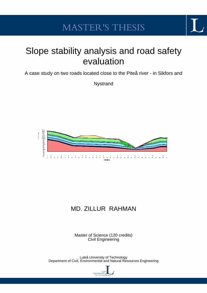
Slope stability analysis and road safetyevaluation

A case study on two roads located close to the Piteå river - in Sikfors and

Nystrand

MD. ZILLUR RAHMAN

Master of Science (120 credits)Civil Engineering

Luleå University of TechnologyDepartment of Civil, Environmental and Natural Resources Engineering

I

SLOPE STABILITY ANALYSIS AND ROAD SAFETY EVALUATION

- A CASE STUDY ON TWO ROADS LOCATED CLOSE TO THE PITEÅ RIVER-IN SIKFORS AND NYSTRAND

MD. ZILLUR RAHMAN

Division of Mining & Geotechnical Engineering

Department of Civil, Environmental and Natural resources engineering

Luleå University of Technology (LTU), Luleå, Sweden

i

Preface At first I express my praise to almighty that the project was completed in

proper time. From my undergraduate studies at the Khulna University of

Engineering & Technology (KUET), Bangladesh, I like Geotechnical

Engineering. I have always loved latest computer software to solving civil

engineering problem.

In November 2011, I met with Nicklas Thun and Göran Pyyny, Geotechnical

specialist, Trafikverket, Luleå, Sweden for the first time and discussed about

master thesis project. In that regard, I would like to thank Nicklas Thun and

Göran Pyyny that gave me the opportunity to work with slope stability analysis

with modern geotechnical software. I’m grateful to them for enduring advice,

kin interest, directing me towards such an interesting problem.

I also, express my profound gratitude, indebtedness and heartiest thanks to

the honorable teacher Dr. Hans Mattsson, Division of Mining and Geotechnical

Engineering, Luleå University of Technology (LTU), Luleå, Sweden, for his

valuable patient advice, sympathetic assistance, constant encouragements,

guidance, co-operation, relatives interest, contribution to new ideas and

supervision of all stages of this project work. His guidance has benefited me

greatly.

This has been a wonderful year for me to have experienced studying in Sweden.

This experience has been more colorful with many friends that support me

during my study. Living in Luleå would never have been as wonderful without

all of you.

Last but not least, I would like to express deep felt gratitude to my family

members and one of my best friends for their continuous support.

Luleå, June 2012

MD. ZILLUR RAHMAN

ii

iii

Abstract This master thesis focuse on natural slope and embankment slope stability

analysis with the Limit Equilibrium Method computer program Slope/W and

the Finite Element Method computer program Plaxis 2D and a comparison of

the analyzed result. The finite element method needs additional information

regarding the potential performance of a slope; just basic parameter

information is needed when using limit equilibrium methods. The results

indicate that it is important to use the effective shear strength characterization

of the soil when performing the slope stability analysis. A distinction should be

made between drained and undrained strength of cohesive materials. Shortly,

drained condition refers to the condition where drainage is allowed, while

undrained condition refers to the condition where drainage is restricted. Most

likely the worst case scenario occurs when the river water level is increased

rapidly, and then quickly drops while the water table in the embankment is

retained on an extremely high level so that the low effective stresses might lead

to failure. The existence of trivial failure surfaces is a large problem in stability

analysis of natural slopes, especially in the Plaxis 2D program. We tried to

avoid these types of failure. In Slope/W analysis we consider critical slip

surface failure. If the critical failure is trivial, then we consider the secondary

failure. In Plaxis 2D analysis, additional displacements are generated during a

Safety calculation. The total incremental displacements in the final step (at

failure) give an indication of the likely failure mechanism.

iv

v

Table of Contents Preface ........................................................................................................................................................... i

Abstract ........................................................................................................................................................ iii

1 INTRODUCTION .......................................................................................................................................... 1

2 BACKGROUND ............................................................................................................................................ 3

2.1 Sikfors ............................................................................................................................................. 3

2.2 Nystrand ......................................................................................................................................... 4

3 OBJECTIVES ........................................................................................................................................ 5

3.1 Nystrand ......................................................................................................................................... 5

3.2 Sikfors ............................................................................................................................................. 5

4 LITERATURE REVIEW ....................................................................................................................... 7

4.1 Ground Investigations ................................................................................................................ 7

4.2 Geotechnical Parameters .......................................................................................................... 7

4.2.1 Unit weight ............................................................................................................................. 7

4.2.2 Cohesion ................................................................................................................................. 7

4.2.3 Friction Angle ........................................................................................................................ 8

4.2.4 Young's Modulus of Soil .................................................................................................... 8

4.3 Type of soil ..................................................................................................................................... 8

4.3.1 Sand .............................................................................................................................................. 8

4.3.2 Clay ............................................................................................................................................... 8

4.3.3 Silt................................................................................................................................................. 8

4.3.4 Silty clay ....................................................................................................................................... 9

4.3.5 Sandy clay ..................................................................................................................................... 9

4.4 Basic Requirement for Slope Stability Analysis ................................................................. 9

4.5 Drained and Undrained Strength......................................................................................... 10

4.5.1 Analyses of Drained Conditions ................................................................................................. 11

4.5.2 Analyses of Undrained Conditions ............................................................................................. 12

4.6 Short-Term Analyses ......................................................................................................................... 12

4.7 Long-Term Analyses .......................................................................................................................... 12

4.8 Pore Water Pressures ....................................................................................................................... 13

4.9 Soil Property Evaluation .................................................................................................................... 13

4.10 Circular Slip Surface ........................................................................................................................ 14

4.11 Factor of Safety ............................................................................................................................... 14

vi

4.12 Traffic load ...................................................................................................................................... 15

4.13 Numerical analysis ................................................................................................................. 15

5 METHODOLOGY ................................................................................................................................ 17

5.1 Slope/W ........................................................................................................................................ 17

5.1.1 Limit Equilibrium Methods ............................................................................................. 17

5.1.2 Defining the Problem ................................................................................................................. 17

5.1.3 Modeling .................................................................................................................................... 18

5.1.4 Analysis Type ...................................................................................................................... 19

5.1.5 Slip Surface for Circular Failure Model ...................................................................................... 20

5.1.6 Verification and Computation .................................................................................................... 21

5.2 Plaxis 2D....................................................................................................................................... 21

5.2.1 Finite Element Modeling .................................................................................................. 21

5.2.2 Mesh Generation and Boundary Conditions ............................................................ 21

5.2.3 Material Model .................................................................................................................... 22

5.2.4 Analysis Type ...................................................................................................................... 22

6 RESULT AND DISCUSSION ........................................................................................................... 23

6.1.1 Sikfors Stora ............................................................................................................................ 24

6.1.1.1 Section B1/B2 .......................................................................................................................... 25

6.1.1.2 Section C1/C2 .......................................................................................................................... 28

6.1.2 Sikfors Ravinen ............................................................................................................................... 29

6.1.2.1 Section D1/D2 ......................................................................................................................... 29

6.1.1.2 Section D.1B/D.2B ................................................................................................................... 31

6.1.2.3 Section E1B/E2B ...................................................................................................................... 32

6.1.3 Sikfors Camping.............................................................................................................................. 33

6.1.3.1 Section F.1/F.2 ........................................................................................................................ 33

6.2 Nystrand ............................................................................................................................................ 34

6.2.1 Section N1/N1b .......................................................................................................................... 35

6.2.2 Section N2 .................................................................................................................................. 36

7 CONCLUSIONS .................................................................................................................................. 37

8 REFERENCES .................................................................................................................................... 39

Appendix A .................................................................................................................................................. 41

Appendix B .................................................................................................................................................. 63

Appendix C ................................................................................................................................................ 101

1

1 INTRODUCTION Evaluating the stability of slopes in soil is an important, interesting, and

challenging aspect of civil engineering. Slope instability is a geo-dynamic

process that naturally shapes up the geo-morphology of the earth. However,

they are a major concern when those unstable slopes would have an effect on

the safety of people and property. Concerns with slope stability have driven

some of the most important advances in our understanding of the complex

behavior of soils. Extensive engineering and research studies performed over

the past 70 years provide a sound set of soil mechanical principles with which

to attack practical problems of slope stability.

Over the past decades, experience with the behavior of slopes, and often with

their failure, has led to development of improved understanding of the changes

in soil properties that can occur over time, recognition of the requirements and

the limitations of laboratory and in situ testing for evaluating soil strengths,

development of new and more effective types of instrumentation to observe the

behavior of slopes, improved understanding of the principles of soil mechanics

that connect soil behavior to slope stability, and improved analytical

procedures augmented by extensive examination of the mechanics of slope

stability analyses, detailed comparisons with field behavior, and use of

computers to perform thorough analyses. Through these advances, the art of

slope stability evaluation has entered a more mature phase, where experience

and judgment, which continue to be of prime importance, have been combined

with improved understanding and rational methods to improve the level of

confidence that is achievable through systematic observation, testing, and

analysis.

This thesis provides the general background information required for slope

stability analysis, suitable methods of analysis with the use of computers, and

examples of common stability problems in the location of the places Sikfors

and Nystrand in North Sweden.

2

3

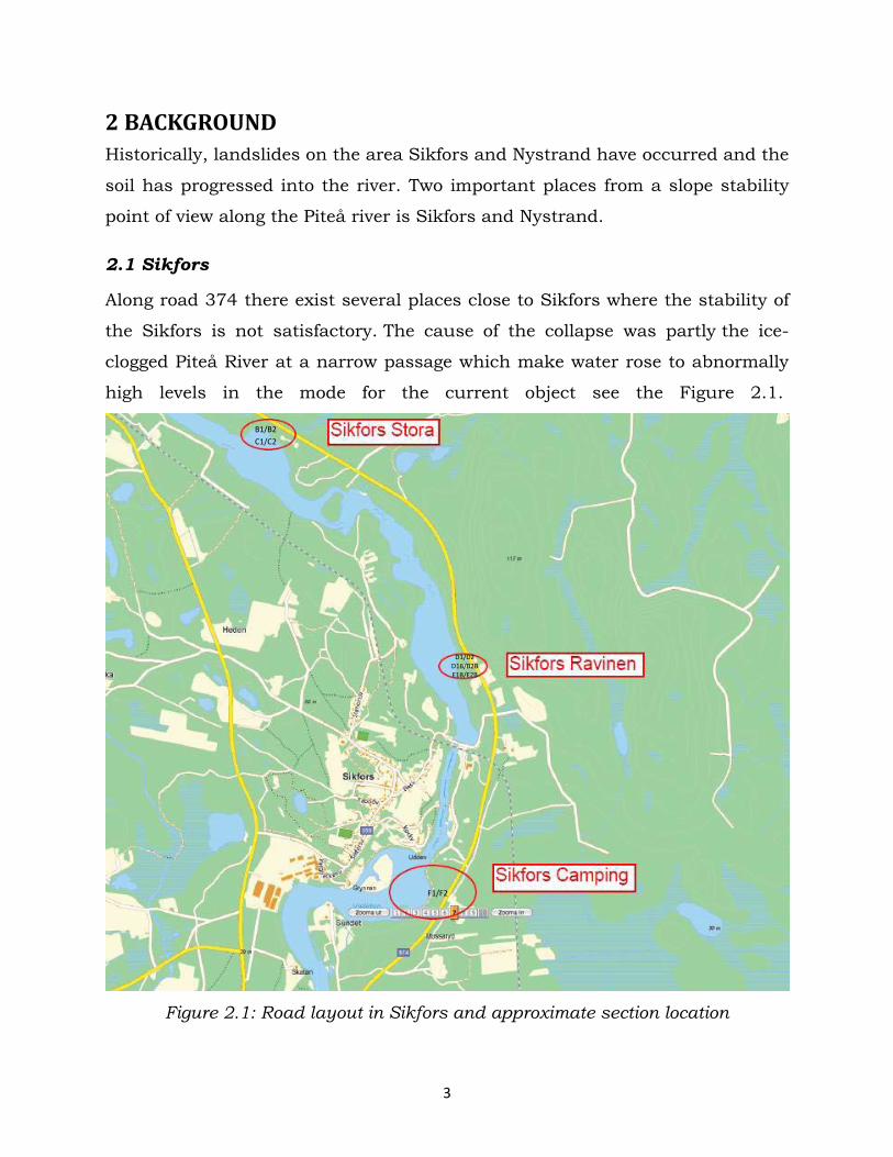
2 BACKGROUND Historically, landslides on the area Sikfors and Nystrand have occurred and the

soil has progressed into the river. Two important places from a slope stability

point of view along the Piteå river is Sikfors and Nystrand.

2.1 Sikfors

Along road 374 there exist several places close to Sikfors where the stability of

the Sikfors is not satisfactory. The cause of the collapse was partly the ice-

clogged Piteå River at a narrow passage which make water rose to abnormally

high levels in the mode for the current object see the Figure 2.1.

Figure 2.1: Road layout in Sikfors and approximate section location

B1/B2 C1/C2

F1/F2

D1/D2 D1B/B2B E1B/E2B

4

The landslide took away about 25 m of the ground surface, which resulted in

that the road were 40 meters closer to the river. After the landslide,

inclinometers and extensometers were installed to control any further

movement. Alarms have been linked via the GSM network. Reports have been

sended directly to the control center (TIC). The stability is poor close to the river

but the road is still expected to have a safe distance to the river. This applies to

a direct landslide. However, it is difficult to predict what will happen if another

ice plug occur.

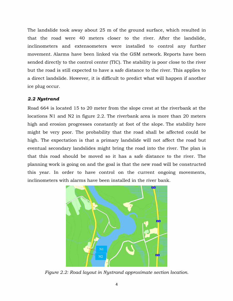
2.2 Nystrand

Road 664 is located 15 to 20 meter from the slope crest at the riverbank at the

locations N1 and N2 in figure 2.2. The riverbank area is more than 20 meters

high and erosion progresses constantly at foot of the slope. The stability here

might be very poor. The probability that the road shall be affected could be

high. The expectation is that a primary landslide will not affect the road but

eventual secondary landslides might bring the road into the river. The plan is

that this road should be moved so it has a safe distance to the river. The

planning work is going on and the goal is that the new road will be constructed

this year. In order to have control on the current ongoing movements,

inclinometers with alarms have been installed in the river bank.

Figure 2.2: Road layout in Nystrand approximate section location.

5

3 OBJECTIVES

The primary purpose of slope analysis in many engineering applications is to

contribute to the road safety analysis. Preliminary analyses assist in the

identification of critical geological, material, environmental and economic

parameters. Therefore the results are of value in planning detailed

investigations of major projects. Subsequent analyses enable an understanding

of the nature, magnitude and frequency of slope problems that may require to

be solved. Evaluation of slope stability is often an inter-disciplinary effort

requiring contributions from engineering geology, soil mechanics and rock

mechanics. In this project the stability and the safety of a road will be

evaluated at two different locations close to the Piteå river; Nystrand and

Sikfors

3.1 Nystrand

At Nystrand the following points will be considered:

Stability calculations with Slope/W and Plaxis 2D to find out factors of

safety (FoS) compare the result with Novapoint GS Stability analysis

Determination of critical failure surface of the slope

Sensitivity analysis (cohesion and friction angle)

3.2 Sikfors

At Sikfors the followings point will be considered:

Stability calculations with Slope/W and Plaxis 2D to obtain factors of

safety (FoS) compare the result with Novapoint GS Stability analysis

Determination of critical failure surface of the slope

Determination of effects on slope stability in the case when the river

water level goes up and then down but the embankment water level are

constantly high

6

7

4 LITERATURE REVIEW

4.1 Ground Investigations

Before any further examination of an existing slope, or the ground onto which a

slope is to be built, essential borehole information must be obtained. This

information will give details of the strata, moisture content and the standing

water level. Also, the presence of any particular plastic layer along which shear

could more easily take place will be noted.

Ground investigations also include:

In-situ and laboratory tests

Aerial photographs

Study of geological maps and memoirs to indicate probable soil

conditions

Visiting and observing the slope

For the study in this thesis, field investigations have been done by Tyrens AB

and they used cone penetration test (CPT) for evaluation geotechnical

parameters.

4.2 Geotechnical Parameters

Before a geotechnical analysis can be performed, the parameters values needed

in the analysis must be determined.

4.2.1 Unit weight

Unit weight of a soil mass is the ratio of the total weight of the soil to the total

volume of the soil. Unit weight, γ, is usually determined in the laboratory by

measuring the weight and volume of a relatively undisturbed soil sample

obtained from the field. Measuring unit weight of soil directly in the field might

be done by sand cone test, rubber balloon or nuclear densiometer. We will use

unit weights presented in a report by Tyrens AB.

4.2.2 Cohesion

Cohesion, c, is usually determined in the laboratory from the Direct Shear

Test. Unconfined Compressive Strength Suc can be determined in the laboratory

8

using the Triaxial Test or the Unconfined Compressive Strength Test. There are

also correlations for Suc with shear strength as estimated from the field

using Vane Shear Tests. Tyrens AB has already determined the cohesions for

this project.

4.2.3 Friction Angle

The angle of internal friction, φ, can be determined in the laboratory by the

Direct Shear Test or by Triaxial test. For our analysis we will use values

determined by Tyrens AB.

4.2.4 Young's Modulus of Soil

Young’s soil modulus, Es, may be estimated from empirical correlations,

laboratory test results on undisturbed specimens and results of field tests.

Laboratory test that might be used to estimate the soil modulus is the triaxial

test. For our analysis we will use values determined by Tyrens AB.

4.3 Type of soil

Geotechnical engineers classify soils, or more properly earth materials, for their

properties relative to foundation support or use as building material. These

systems are designed to predict some of the engineering properties and

behavior of a soil based on a few simple laboratory or field tests

4.3.1 Sand Soil material that contains 85% or more sand; the percentage of silt plus 1.5

times the percentage of clay does not exceed 15 (CSSC; USDA).

4.3.2 Clay Soil material that contains 40% or more clay and 40% or more silt (CSSC;

USDA).

4.3.3 Silt Soil material that contains 80% or more silt and less than 12% clay (CSSC;

USDA).

9

4.3.4 Silty clay Soil material that contains 40% or more clay and 35% or more silt (CSSC;

USDA).

4.3.5 Sandy clay Soil material that contains 7 to 27% clay, 28 to 50% silt, and less than 52%

sand (CSSC; USDA).

4.4 Basic Requirement for Slope Stability Analysis

Whether slope stability analyses are performed for drained conditions or

undrained conditions, the most basic requirement is that equilibrium must be

satisfied in terms of total stresses. All body forces (weights), and all external

loads, including those due to water pressures acting on external boundaries,

must be included in the analysis. These analyses provide two useful results: (1)

the total normal stress on the shear surface and (2) the shear stress required

for equilibrium.

The factor of safety for the shear surface is the ratio of the shear strength of the

soil divided by the shear stress required for equilibrium. The normal stresses

along the slip surface are needed to evaluate the shear strength: except for

soils with φ = 0, the shear strength depends on the normal stress on the

potential plane of failure.

In effective stress analyses, the pore pressures along the shear surface are

subtracted from the total stresses to determine effective normal stresses, which

are used to evaluate shear strengths. Therefore, to perform effective stress

analyses, it is necessary to know (or to estimate) the pore pressures at every

point along the shear surface. These pore pressures can be evaluated with

relatively good accuracy for drained conditions, where their values are

determined by hydrostatic or steady seepage boundary conditions. Pore

pressures can seldom be evaluated accurately for undrained conditions, where

their values are determined by the response of the soil to external loads.

10

In total stress analyses, pore pressures are not subtracted from the total

stresses, because shear strengths are related to total stresses. Therefore, it is

not necessary to evaluate and subtract pore pressures to perform total stress

analyses. Total stress analyses are applicable only to undrained conditions.

The basic premise of total stress analysis is this: the pore pressures due to

undrained loading are determined by the behavior of the soil. For a given value

of total stress on the potential failure plane, there is a unique value of pore

pressure and therefore a unique value of effective stress. Thus, although it is

true that shear strength is really controlled by effective stress, it is possible for

the undrained condition to relate shear strength to total normal stress,

because effective stress and total stress are uniquely related for the undrained

condition. Clearly, this line of reasoning does not apply to drained conditions,

where pore pressures are controlled by hydraulic boundary conditions rather

than the response of the soil to external loads.

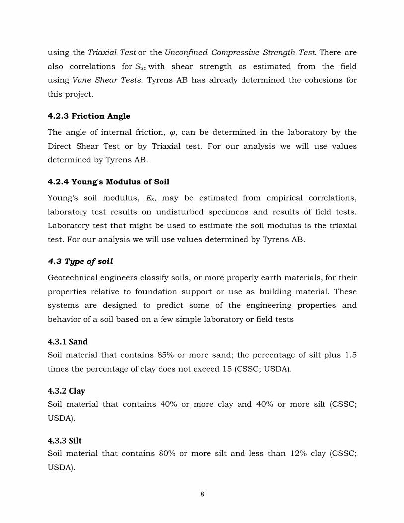
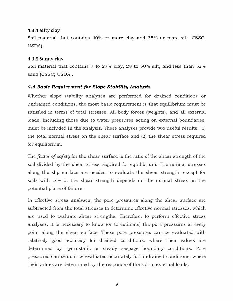
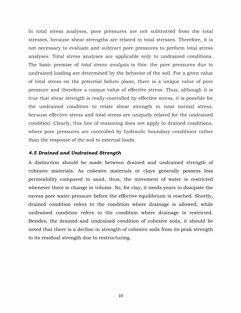
4.5 Drained and Undrained Strength

A distinction should be made between drained and undrained strength of

cohesive materials. As cohesive materials or clays generally possess less

permeability compared to sand, thus, the movement of water is restricted

whenever there is change in volume. So, for clay, it needs years to dissipate the

excess pore water pressure before the effective equilibrium is reached. Shortly,

drained condition refers to the condition where drainage is allowed, while

undrained condition refers to the condition where drainage is restricted.

Besides, the drained and undrained condition of cohesive soils, it should be

noted that there is a decline in strength of cohesive soils from its peak strength

to its residual strength due to restructuring.

11

Figure 4.1a: Results of Triaxial Undrained Tests on Saturated Clay

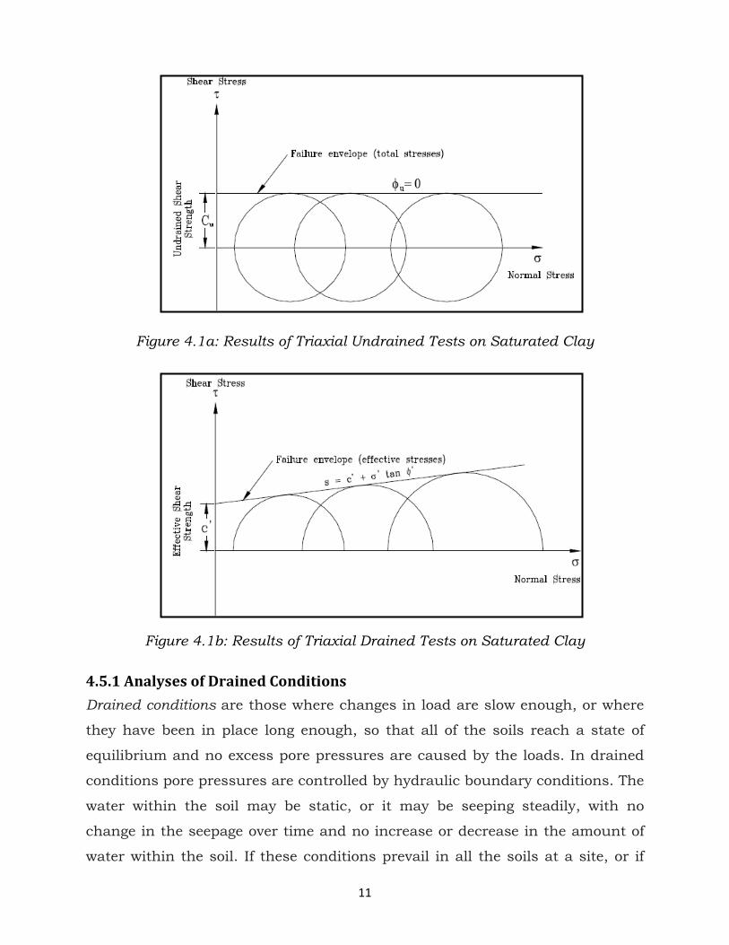
Figure 4.1b: Results of Triaxial Drained Tests on Saturated Clay

4.5.1 Analyses of Drained Conditions Drained conditions are those where changes in load are slow enough, or where

they have been in place long enough, so that all of the soils reach a state of

equilibrium and no excess pore pressures are caused by the loads. In drained

conditions pore pressures are controlled by hydraulic boundary conditions. The

water within the soil may be static, or it may be seeping steadily, with no

change in the seepage over time and no increase or decrease in the amount of

water within the soil. If these conditions prevail in all the soils at a site, or if

12

the conditions at a site can reasonably be approximated by these conditions, a

drained analysis is appropriate. A drained analysis is performed using:

• Total unit weights

• Effective stress shear strength parameters

• Pore pressures determined from hydrostatic water levels or steady

seepage analyses

4.5.2 Analyses of Undrained Conditions Undrained conditions are those where changes in loads occur more rapidly than

water can flow in or out of the soil. The pore pressures are controlled by the

behavior of the soil in response to changes in external loads. If these conditions

prevail in the soils at a site, or if the conditions at a site can reasonably be

approximated by these conditions, an undrained analysis is appropriate. An

undrained analysis is performed using:

• Total unit weights

• Total stress shear strength parameters

4.6 Short-Term Analyses Short term refers to conditions during or following construction—the time

immediately following the change in load. For example, if constructing a sand

embankment on a clay foundation takes two months, the short-term condition

for the embankment would be the end of construction, or two months. Within

this period of time, it would be a reasonable approximation that no drainage

would occur in the clay foundation, whereas the sand embankment would be

fully drained.

4.7 Long-Term Analyses After a period of time, the clay foundation would reach a drained condition,

and the analysis for this condition would be performed as discussed earlier

under ‘‘Analyses of Drained Conditions’’, because long term and drained

conditions carry exactly the same meaning. Both of these terms refer to the

condition where drainage equilibrium has been reached and there are no

excess pore pressures due to external loads.

13

4.8 Pore Water Pressures For effective stress analyses the basis for pore water pressures should be

described. If pore water pressures are based on measurements of groundwater

levels in bore holes or with piezometers, the measured data should be

described and summarized in appropriate figures or tables. If seepage analyses

are performed to compute the pore water pressures, the method of analysis,

including computer software, which was used, should be described. Also, for

such analyses the soil properties and boundary conditions as well as any

assumptions used in the analyses should be described. Soil properties should

include the hydraulic conductivities. Appropriate flow nets or contours of pore

water pressure, total head, or pressure head should be presented to summarize

the results of the analyses.

4.9 Soil Property Evaluation The basis for the soil properties used in a stability evaluation should be

described and appropriate laboratory test data should be presented. If

properties are estimated based on experience, or using correlations with other

soil properties or from data from similar sites, this should be explained.

Results of laboratory tests should be summarized to include index properties,

water content, and unit weights. For compacted soils, suitable summaries of

compaction moisture–density data are useful. A summary of shear strength

properties is particularly important and should include both the original data

and the shear strength envelopes used for analyses (Mohr–Coulomb diagrams,

modified Mohr–Coulomb diagrams). The principal laboratory data that are used

in slope stability analyses are the unit weights and shear strength envelopes. If

many more extensive laboratory data are available, the information can be

presented separately from the stability analyses in other sections, chapters, or

separate reports. Only the summaries of shear strength and unit weight

information need to be presented with the stability evaluation in such cases.

14

4.10 Circular Slip Surface Inherent in limit equilibrium stability analyses is the requirement to analyze

many trials slip surfaces and find the slip surface that gives the lowest factor of

safety. Included in this trial approach is the form of the slip surface; that is,

whether it is circular, piece-wise linear or some combination of curved and

linear segments. Slope/W has a variety of options for specifying trial slip

surfaces. The position of the critical slip surface is affected by the soil strength

properties. The position of the critical slip surface for a purely frictional soil (c =

0) is radically different than for a soil assigned untrained strength (φ = 0). This

complicates the situation, because it means that in order to find the position of

the critical slip surface, it is necessary to accurately define the soil properties

in terms of effective strength parameters.

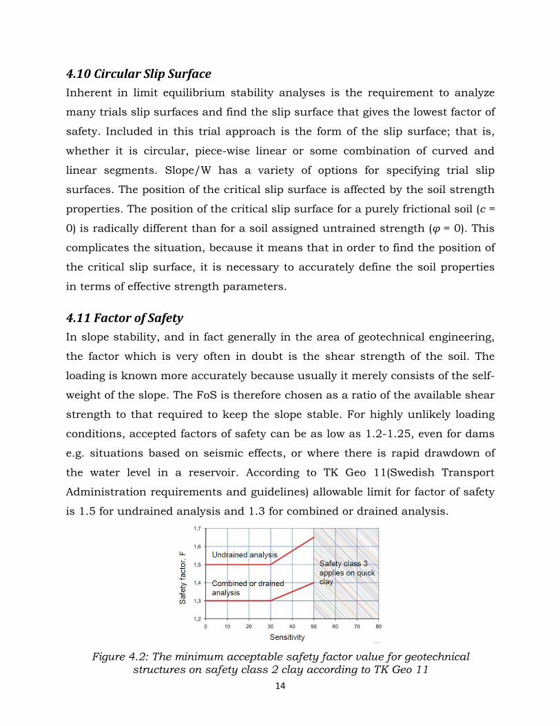
4.11 Factor of Safety In slope stability, and in fact generally in the area of geotechnical engineering,

the factor which is very often in doubt is the shear strength of the soil. The

loading is known more accurately because usually it merely consists of the self-

weight of the slope. The FoS is therefore chosen as a ratio of the available shear

strength to that required to keep the slope stable. For highly unlikely loading

conditions, accepted factors of safety can be as low as 1.2-1.25, even for dams

e.g. situations based on seismic effects, or where there is rapid drawdown of

the water level in a reservoir. According to TK Geo 11(Swedish Transport

Administration requirements and guidelines) allowable limit for factor of safety

is 1.5 for undrained analysis and 1.3 for combined or drained analysis.

Figure 4.2: The minimum acceptable safety factor value for geotechnical

structures on safety class 2 clay according to TK Geo 11

15

4.12 Traffic load Traffic load refers to the action of the traffic on the carriageway or railway

structure. Action distribution shall be taken into consideration using an elastic

theoretical based method. Where there are low permeable soils the traffic load

is to be reduced for drained and combined analysis. Normally the traffic load

can be ignored for combined analysis and drained analysis in the above

conditions. Account must be taken of the vehicles and other equipment used in

the execution phase.

Design using partial factors. The characteristic surface load for traffic shall be:

15 kN/m2 for design situations where the critical failure surfaces are short

10 kN/m2 for design situations where the critical failure surfaces are long

Design using characteristic values. The characteristic surface load for traffic shall be: 20 kN/m2 for design situations where the critical failure surfaces are

short 13 kN/m2 for design situations where the critical failure surfaces are

long

4.13 Numerical analysis

Slope stability analyses can be performed using deterministic or probabilistic

input parameters. Plaxis 2D and Geostudio (SLOPE/W) can model

heterogeneous soil types, complex stratigraphic and slip surface geometry, and

variable pore-water pressure conditions using a large selection of soil models.

16

17

5 METHODOLOGY

Many different solution techniques for slope stability analyses have been

developed over the years. Analyze of slope stability is one of the oldest type of

numerical analysis in geotechnical engineering. In this project we will use both

Limit Equilibrium Method and Finite Element Method for our analysis. Two

modern geotechnical software programs are utilized, i.e. Slope/W and Plaxis

2D.

5.1 Slope/W

5.1.1 Limit Equilibrium Methods

Modern limit equilibrium software is making it possible to handle ever-

increasing complexity within an analysis. It is now possible to deal with

complex stratigraphy, highly irregular pore-water pressure conditions, and

various linear and nonlinear shear strength models, almost any kind of slip

surface shape, distributed or concentrated loads, and structural reinforcement.

Limit equilibrium formulations based on the method of slices are also being

applied more and more to the stability analysis of structures such as tie-back

walls, nail or fabric reinforced slopes, and even the sliding stability of

structures subjected to high horizontal loading arising, for example, from ice

flows.

5.1.2 Defining the Problem A limit equilibrium analysis was carried out using the Slope/W software for the

slope stability of the natural slope. The geometry was created in .dxt format

and imported into the Slope/W program. The analysis type is then selected and

it is determined that failure will follow a right to left path. The Morgenstern-

Price analysis and half-sine function was selected but the software also gives

the result of factor of safety for Ordinary, Bishop and Janbu analysis type.

18

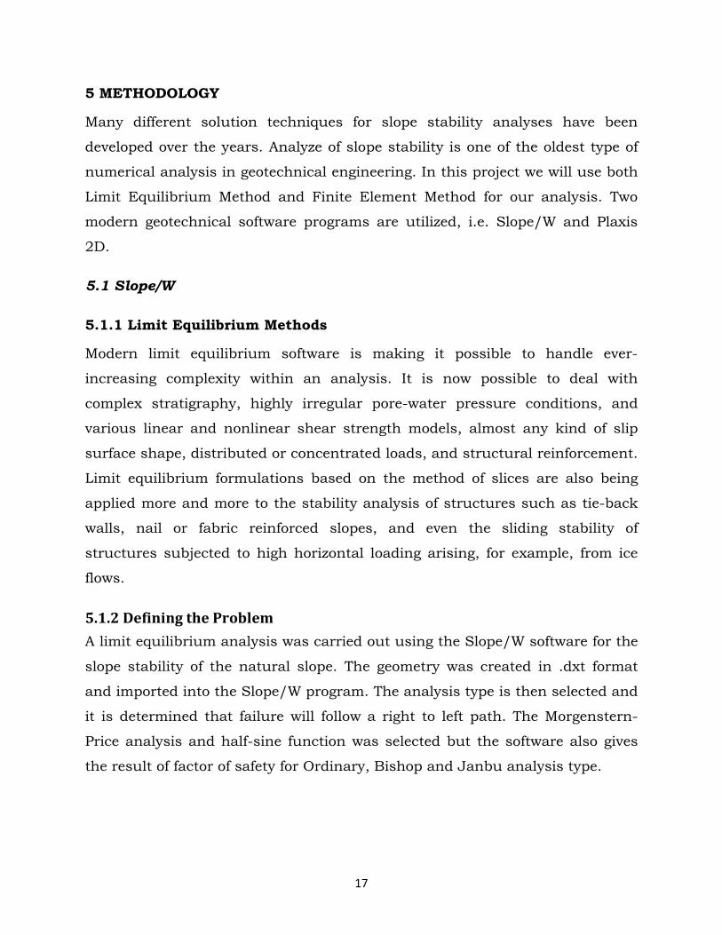
5.1.3 Modeling The most common way of describing the shear strength of geotechnical

materials is by Coulomb’s equation which is:

τ = c + σn´tanφ … … … … … … … (5.1)

where, τ is shear strength (i.e., shear at failure), c is cohesion, σ´n is normal

stress on shear plane, and φ is angle of internal friction. The equation 5.1

represents a straight line on shear strength versus normal stress plot (Figure

5.1). The intercept on the shear strength axis is the cohesion c and the slope of

the line is the angle of internal friction φ.

Figure 5.1: Graphical representation of Coulomb shear strength equation

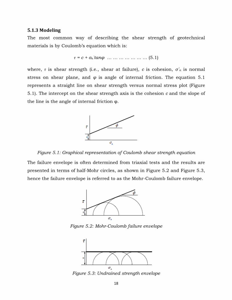
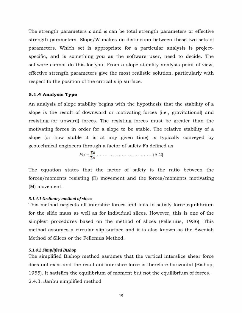
The failure envelope is often determined from triaxial tests and the results are

presented in terms of half-Mohr circles, as shown in Figure 5.2 and Figure 5.3,

hence the failure envelope is referred to as the Mohr-Coulomb failure envelope.

Figure 5.2: Mohr-Coulomb failure envelope

Figure 5.3: Undrained strength envelope

19

The strength parameters c and φ can be total strength parameters or effective

strength parameters. Slope/W makes no distinction between these two sets of

parameters. Which set is appropriate for a particular analysis is project-

specific, and is something you as the software user, need to decide. The

software cannot do this for you. From a slope stability analysis point of view,

effective strength parameters give the most realistic solution, particularly with

respect to the position of the critical slip surface.

5.1.4 Analysis Type

An analysis of slope stability begins with the hypothesis that the stability of a

slope is the result of downward or motivating forces (i.e., gravitational) and

resisting (or upward) forces. The resisting forces must be greater than the

motivating forces in order for a slope to be stable. The relative stability of a

slope (or how stable it is at any given time) is typically conveyed by

geotechnical engineers through a factor of safety Fs defined as

Fs = … … … … … … … … … (5.2)

The equation states that the factor of safety is the ratio between the

forces/moments resisting (R) movement and the forces/moments motivating

(M) movement.

5.1.4.1 Ordinary method of slices This method neglects all interslice forces and fails to satisfy force equilibrium

for the slide mass as well as for individual slices. However, this is one of the

simplest procedures based on the method of slices (Fellenius, 1936). This

method assumes a circular slip surface and it is also known as the Swedish

Method of Slices or the Fellenius Method.

5.1.4.2 Simplified Bishop The simplified Bishop method assumes that the vertical interslice shear force

does not exist and the resultant interslice force is therefore horizontal (Bishop,

1955). It satisfies the equilibrium of moment but not the equilibrium of forces.

2.4.3. Janbu simplified method

20

This method uses the horizontal forces equilibrium equation to obtain the

factor of safety. It does not include interslice forces in the analysis but account

for its effect using a correction factor. The correction factor is related to

cohesion, angle of internal friction and the shape of the failure surface (Janbu

et al., 1956).

5.1.4.3 Spencer Method This is a very accurate method which satisfies both equilibrium of forces and

moments and it works for any shape of slip surface. The basic assumption

used in this method is that the inclinations of the side forces are the same for

all the slices.

5.1.4.4 Morgenstern and Price Morgenstern and Price proposed a method that is similar to Spencer's method,

except that the inclination of the interslice resultant force is assumed to vary

according to a "portion" of an arbitrary function. This method allows one to

specify different types of interslice force function (Morgenstern & Price, 1965).

5.1.4.5 General Limit Equilibrium This method can be used to satisfy either force or moment equilibrium, or if

required, just the force equilibrium conditions. It encompasses most of the

assumptions used by various methods and may be used to analyze circular

and noncircular failure surfaces (Ferdlund, Krahn, & Pufahl, 1981).

5.1.5 Slip Surface for Circular Failure Model After the material input and pore pressure was assigned, a slip surface was

defined. The analyses were performed for two failure models namely the

circular failure model and block failure model. There were several methods for

defining the slip surface for the circular failure but the entry and exit method

was selected. One of the problems with the other methods is how to visualize

the extents or the range of the trial slip surface. This difficulty is solved by the

entry and exit method because it specifies the location where the trial slip

surfaces should enter the ground surface and where they should exit.

21

5.1.6 Verification and Computation When the slip surface has been specified, then Slope/W runs several checks to

verify the input data using the verify/optimize data command in the Tools

menu. When the verification is completed and there are no errors, then

Slope/W computes the factor of safety using the method of slice selected. The

minimum factor of safety is obtained for that particular analysis and its

corresponding critical slip surface is displayed.

5.2 Plaxis 2D

5.2.1 Finite Element Modeling

The finite element program Plaxis 2D was used for evaluating the stability of

natural slope. The natural slope cross-section utilized for the numerical model

is presented in Appendix B.

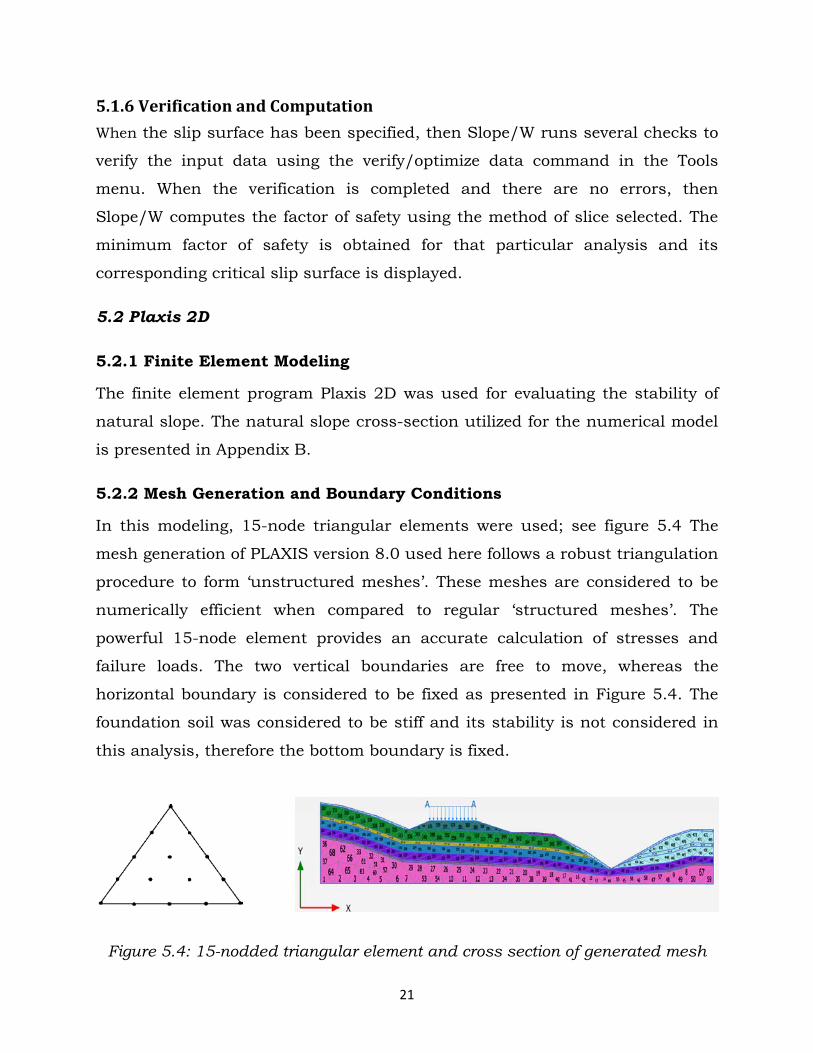
5.2.2 Mesh Generation and Boundary Conditions

In this modeling, 15-node triangular elements were used; see figure 5.4 The

mesh generation of PLAXIS version 8.0 used here follows a robust triangulation

procedure to form ‘unstructured meshes’. These meshes are considered to be

numerically efficient when compared to regular ‘structured meshes’. The

powerful 15-node element provides an accurate calculation of stresses and

failure loads. The two vertical boundaries are free to move, whereas the

horizontal boundary is considered to be fixed as presented in Figure 5.4. The

foundation soil was considered to be stiff and its stability is not considered in

this analysis, therefore the bottom boundary is fixed.

Figure 5.4: 15-nodded triangular element and cross section of generated mesh

22

5.2.3 Material Model

The Mohr–Coulomb model was used for this analysis. This model involves five

parameters, namely Young’s modulus, E, Poisson’s ratio, ν, the cohesion, c, the

friction angle, φ, and the dilatancy angle, ψ. In this case dilatancy angle was

assumed to be zero, since it is close to zero for clay and for sands with a

friction angle less than 380 (Lenita,T.).

5.2.4 Analysis Type

The factor of safety in PLAXIS was computed using Phi-c reduction at each case

of slope modeling. In this type of calculation the load advancement number of

steps procedure is followed. The incremental multiplier Msf is used to specify

the increment of the strength reduction of the first calculation step. The

strength parameters are reduced successively in each step until all the steps

have been performed. The final step should result in a fully developed failure

mechanism, if not the calculation must be repeated with a larger number of

additional steps. Once the failure mechanism is reached, the factor of safety is

given by (PLAXIS 2D manual)

SF = = ΣMsf value of Msf at failure … … … (5.3)

23

6 RESULT AND DISCUSSION

The stability of natural slopes ware analyzed for drained and undrained

conditions by using both finite the element program Plaxis 2D and Limit

Equilibrium Methods (LEM) slope stability software Slope/W. Results from

slope stability analysis are presented in Appendix A and Appendix B. Appendix

A shows the safety factors calculated by slope/W utilizing the Morgenstern-

Price methods, Ordinary method, modified Bishop Method and Janbu method

and Appendix B presents output of the total incremental displacements output

from Plaxis 2D for both drained and undrained conditions. A distinction should

be made between drained and undrained strength of cohesive materials. As

cohesive materials or clays generally possess less permeability compared to

sand, thus, the movement of water is restricted whenever there is change in

volume. So, for clay, it takes years to dissipate the excess pore water pressure

before the effective equilibrium is reached. Shortly, drained condition refers to

the condition where drainage is allowed, while undrained condition refers to

the condition where drainage is restricted. Besides, the drained and undrained

condition of cohesive soils, it should be noted that there is a decline in strength

of cohesive soils from its peak strength to its residual strength due to

restructuring.

The existence of trivial failure surface is a large problem in stability analysis of

natural slopes, especially in the Plaxis 2D program. We try to avoid these types

of failure. That’s why we sometimes cut some portions of the slope or use high

strength soil parameters in exposed part, i.e. cohesion, c´ = 100 Kpa, and

friction angle, φ = 450. In Slope/W analysis we consider critical slip surface

failure. If the critical failure is trivial, then we consider the secondary failure

which present in Appendix A. In Plaxis 2D analysis, additional displacements

are generated during a Safety calculation. The total displacements in the final

step (at failure) give an indication of likely failure mechanism. The incremental

displacement curve present in Appendix B. The shading of the total

displacements indicating the most applicable failure mechanism of the

embankment in the final stage.

24

In the calculations, according to Swedish road administration guideline (TK

Geo 11), a traffic load of q = 20 kPa is used for design situations where the

critical failure surfaces are short. Though, the road is relatively far from the

river in all the analysed sections. So, traffic load impact is insignificant.

6.1.1 Sikfors Stora

Landslides on the slope in the area Sikfors Stora occurred very potently and

the soil has progressed into the river. In this area we selected two section B

and section C between the road 374 and the Piteå river for analysis. Soil

properties were evaluated from by CPT sound test result presented in Table

6.1, Table 6.2, Table 6.3 and Table 6.4. The ground water table found in this

area is approximately situated 6 meter below the ground surface at the crest in

the spring season. In the autumn season we found that the groundwater levels

the same as the river level.

Table 6.1: Geotechnical parameters of section B1/B2 for the different layers

Soil

Layer

ɣsat

(KN/m3)

ɣunsat

(KN/m3)

Friction

Angle,

φ (0)

Undrained

Shear Strength,

τ (KPa)

Cohesion

c´ (KPa)

Young’s

Modulus

E (MPa)

Poisson

Ratio,

ν

saSi 17 11.11 34 - 10.0 3.00 0.33

Si 17 11.11 38 - 10.0 2.00 0.33

Table 6.2: Geotechnical parameters of section C1/C2 for different layers

Soil

Layer

ɣsat

(KN/m3)

ɣunsat

(KN/m3)

Friction

Angle,

φ (0)

Undrained

Shear Strength,

τ (KPa)

Cohesion

c´ (KPa)

Young’s

Modulus

E (MPa)

Poisson

Ratio,

ν

Sa/Si 18 12.70 33 - 10 15.90 0.33

Si 15 7.94 28 - 10 19.20 0.33

MSa 18 12.70 34 - - 19.40 0.33

Cl 15 7.94 28 15 - 80 1.5 - 8 2.00 0.33

saSi 18 12.70 35 - 10 39.25 0.33

25

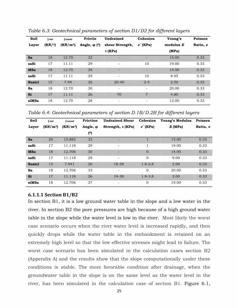
Table 6.3: Geotechnical parameters of section D1/D2 for different layers Soil

Layer

ɣsat

(KN/3)

ɣunsat

(KN/m3)

Frictio

Angle, φ (0)

Undrained

shear Strength,

τ (KPa)

Cohesion

c´ (KPa)

Young’s

modulus E

(MPa)

Poisson

Ratio, ν

Sa 18 12.70 32 - - 15.00 0.33

saSi 17 11.11 29 - 10 19.00 0.33

MSa 18 12.70 30 - - 14.00 0.33

saSi 17 11.11 29 - 10 8.95 0.33

Susicl 15 7.94 26 20-40 2-4 2.50 0.33

Sa 18 12.70 30 - - 20.00 0.33

Si 17 11.11 26 70 7 4.80 0.33

siMSa 18 12.70 28 - - 12.00 0.33

Table 6.4: Geotechnical parameters of section D.1B/D.2B for different layers Soil

Layer

ɣsat

(KN/m3)

ɣunsat

(KN/m3)

Friction

Angle, φ

(0)

Undrained Shear

Strength, τ (KPa)

Cohesion

c´ (KPa)

Young’s Modulus

E (MPa)

Poisson

Ratio, ν

Sa 20 15.882 32 - 1 15.00 0.33

saSi 17 11.118 29 - 1 19.00 0.33

MSa 18 12.706 30 - 0 14.00 0.33

saSi 17 11.118 29 - 0 9.00 0.33

Susicl 15 7.941 26 18-28 1.8-2.8 2.00 0.33

Sa 18 12.706 33 - 0 20.00 0.33

Si 17 11.118 26 19-38 1.9-3.8 3.00 0.33

siMSa 18 12.706 37 - 0 19.00 0.33

6.1.1.1 Section B1/B2 In section B1, it is a low ground water table in the slope and a low water in the

river. In section B2 the pore pressures are high because of a high ground water

table in the slope while the water level is low in the river. Most likely the worst

case scenario occurs when the river water level is increased rapidly, and then

quickly drops while the water table in the embankment is retained on an

extremely high level so that the low effective stresses might lead to failure. The

worst case scenario has been simulated in the calculation cases section B2

(Appendix A) and the results show that the slope computationally under these

conditions is stable. The more favorable condition after drainage, when the

groundwater table in the slope is on the same level as the water level in the

river, has been simulated in the calculation case of section B1. Figure 6.1,

26

1,6

1,65

1,7

1,75

1,8

1,85

1,9

1,95

2

Fact

or o

f Saf

ty (F

oS) >

>>

Change Value >>>

CohesionFriction Angle

-10% Actual +10%

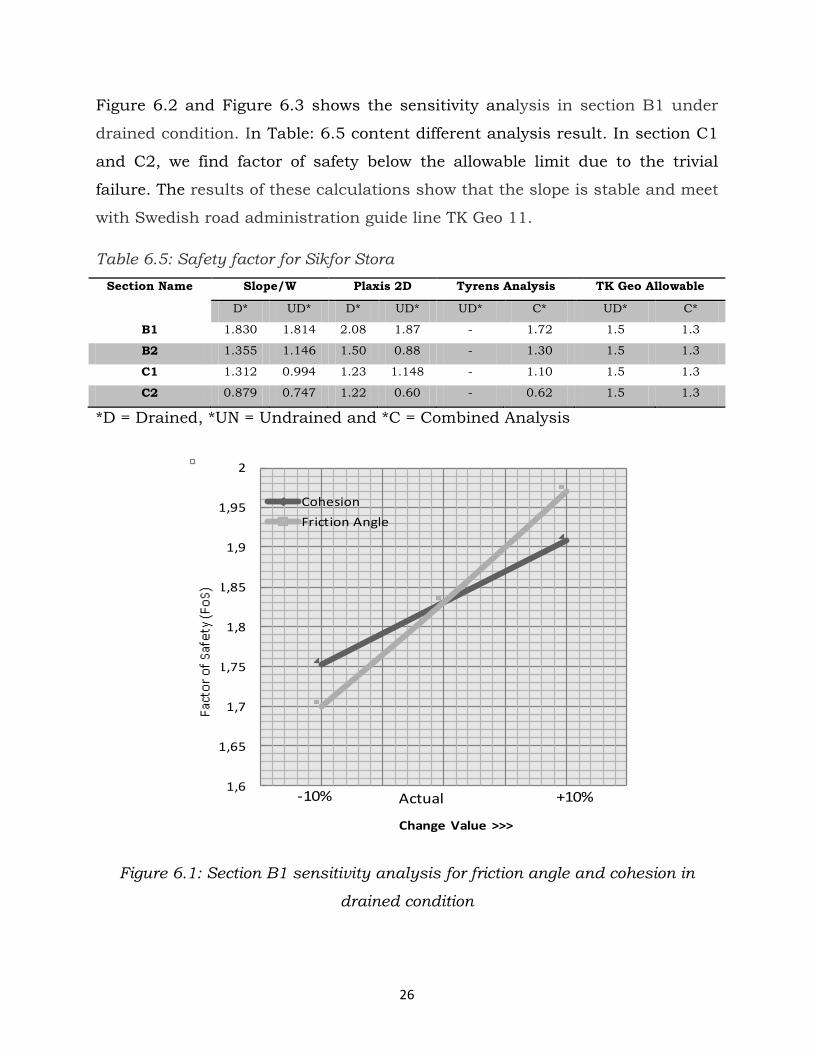
Figure 6.2 and Figure 6.3 shows the sensitivity analysis in section B1 under

drained condition. In Table: 6.5 content different analysis result. In section C1

and C2, we find factor of safety below the allowable limit due to the trivial

failure. The results of these calculations show that the slope is stable and meet

with Swedish road administration guide line TK Geo 11.

Table 6.5: Safety factor for Sikfor Stora Section Name Slope/W Plaxis 2D Tyrens Analysis TK Geo Allowable

D* UD* D* UD* UD* C* UD* C*

B1 1.830 1.814 2.08 1.87 - 1.72 1.5 1.3

B2 1.355 1.146 1.50 0.88 - 1.30 1.5 1.3

C1 1.312 0.994 1.23 1.148 - 1.10 1.5 1.3

C2 0.879 0.747 1.22 0.60 - 0.62 1.5 1.3

*D = Drained, *UN = Undrained and *C = Combined Analysis

Figure 6.1: Section B1 sensitivity analysis for friction angle and cohesion in

drained condition

27

0 75 80 85 90 95 100 105 110

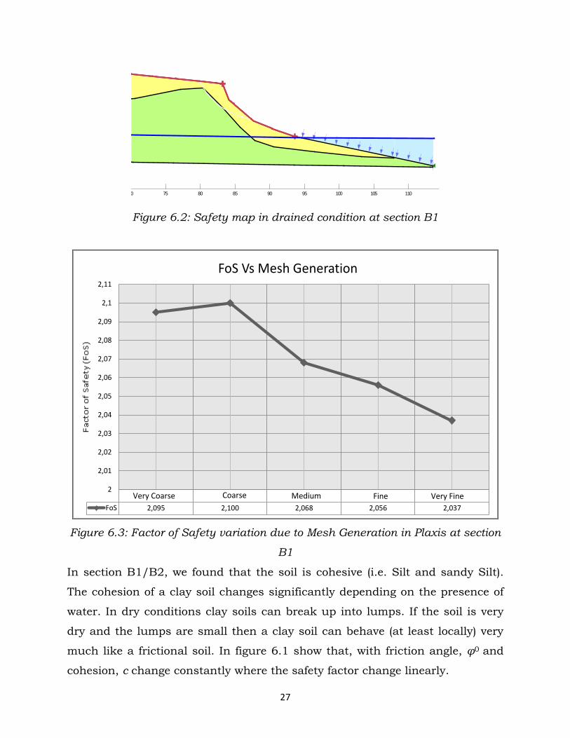
Figure 6.2: Safety map in drained condition at section B1

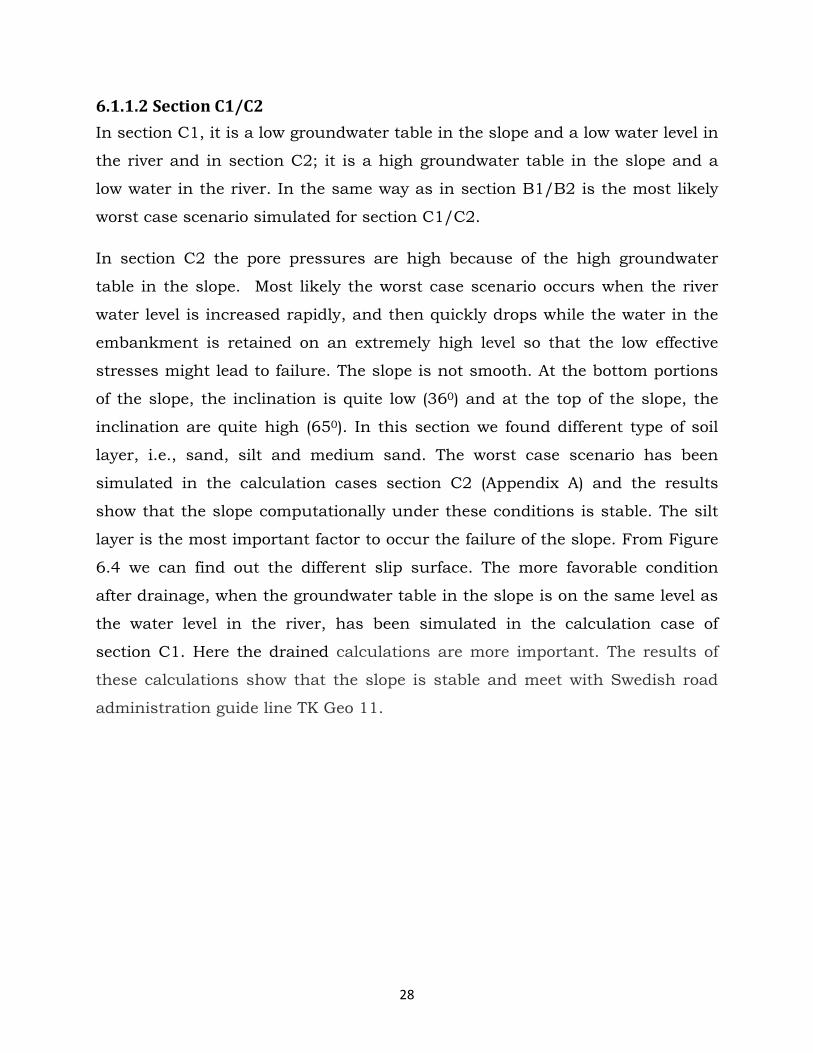
1 2 3 4 5FoS 2,095 2,100 2,068 2,056 2,037

2

2,01

2,02

2,03

2,04

2,05

2,06

2,07

2,08

2,09

2,1

2,11

Foct

or o

f Saf

ety

FoS Vs Mesh Generation

Medium Fine Very FineVery Coarse Coarse

Figure 6.3: Factor of Safety variation due to Mesh Generation in Plaxis at section

B1

In section B1/B2, we found that the soil is cohesive (i.e. Silt and sandy Silt).

The cohesion of a clay soil changes significantly depending on the presence of

water. In dry conditions clay soils can break up into lumps. If the soil is very

dry and the lumps are small then a clay soil can behave (at least locally) very

much like a frictional soil. In figure 6.1 show that, with friction angle, φ0 and

cohesion, c change constantly where the safety factor change linearly.

28

6.1.1.2 Section C1/C2 In section C1, it is a low groundwater table in the slope and a low water level in

the river and in section C2; it is a high groundwater table in the slope and a

low water in the river. In the same way as in section B1/B2 is the most likely

worst case scenario simulated for section C1/C2.

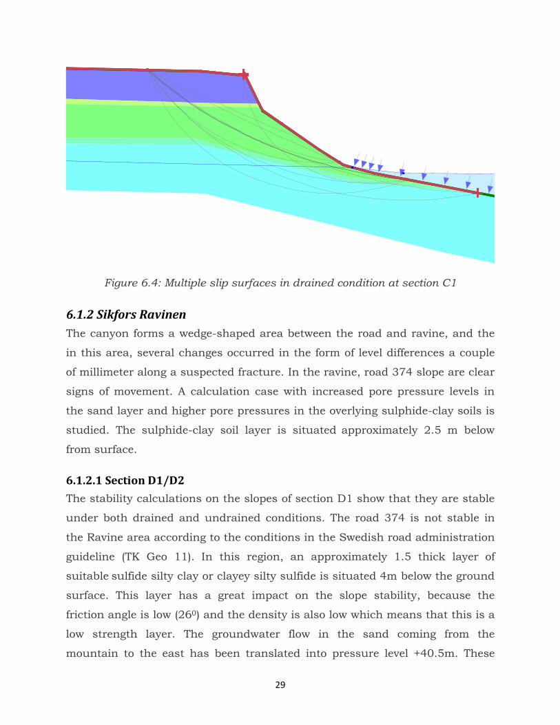
In section C2 the pore pressures are high because of the high groundwater

table in the slope. Most likely the worst case scenario occurs when the river

water level is increased rapidly, and then quickly drops while the water in the

embankment is retained on an extremely high level so that the low effective

stresses might lead to failure. The slope is not smooth. At the bottom portions

of the slope, the inclination is quite low (360) and at the top of the slope, the

inclination are quite high (650). In this section we found different type of soil

layer, i.e., sand, silt and medium sand. The worst case scenario has been

simulated in the calculation cases section C2 (Appendix A) and the results

show that the slope computationally under these conditions is stable. The silt

layer is the most important factor to occur the failure of the slope. From Figure

6.4 we can find out the different slip surface. The more favorable condition

after drainage, when the groundwater table in the slope is on the same level as

the water level in the river, has been simulated in the calculation case of

section C1. Here the drained calculations are more important. The results of

these calculations show that the slope is stable and meet with Swedish road

administration guide line TK Geo 11.

29

Figure 6.4: Multiple slip surfaces in drained condition at section C1

6.1.2 Sikfors Ravinen The canyon forms a wedge-shaped area between the road and ravine, and the

in this area, several changes occurred in the form of level differences a couple

of millimeter along a suspected fracture. In the ravine, road 374 slope are clear

signs of movement. A calculation case with increased pore pressure levels in

the sand layer and higher pore pressures in the overlying sulphide-clay soils is

studied. The sulphide-clay soil layer is situated approximately 2.5 m below

from surface.

6.1.2.1 Section D1/D2 The stability calculations on the slopes of section D1 show that they are stable

under both drained and undrained conditions. The road 374 is not stable in

the Ravine area according to the conditions in the Swedish road administration

guideline (TK Geo 11). In this region, an approximately 1.5 thick layer of

suitable sulfide silty clay or clayey silty sulfide is situated 4m below the ground

surface. This layer has a great impact on the slope stability, because the

friction angle is low (260) and the density is also low which means that this is a

low strength layer. The groundwater flow in the sand coming from the

mountain to the east has been translated into pressure level +40.5m. These

30

Material "Fill Material": UnitWeightMaterial "saSi": Unit WeightMaterial "MSa": Unit WeightMaterial "saSi (2)": UnitWeightMaterial "SusiCl": UnitWeightMaterial "Sa": Unit WeightMaterial "Si": Unit WeightMaterial "siMSa": UnitWeight

Fact

or o

f Saf

ety

Sensitivity Range

1.2

1.22

1.24

1.26

1.28

1.3

1.32

1.34

1.36

0 0.2 0.4 0.6 0.8 1

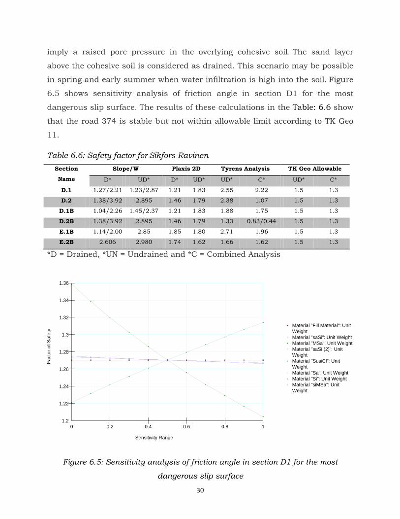
imply a raised pore pressure in the overlying cohesive soil. The sand layer

above the cohesive soil is considered as drained. This scenario may be possible

in spring and early summer when water infiltration is high into the soil. Figure

6.5 shows sensitivity analysis of friction angle in section D1 for the most

dangerous slip surface. The results of these calculations in the Table: 6.6 show

that the road 374 is stable but not within allowable limit according to TK Geo

11.

Table 6.6: Safety factor for Sikfors Ravinen Section

Name

Slope/W Plaxis 2D Tyrens Analysis TK Geo Allowable

D* UD* D* UD* UD* C* UD* C*

D.1 1.27/2.21 1.23/2.87 1.21 1.83 2.55 2.22 1.5 1.3

D.2 1.38/3.92 2.895 1.46 1.79 2.38 1.07 1.5 1.3

D.1B 1.04/2.26 1.45/2.37 1.21 1.83 1.88 1.75 1.5 1.3

D.2B 1.38/3.92 2.895 1.46 1.79 1.33 0.83/0.44 1.5 1.3

E.1B 1.14/2.00 2.85 1.85 1.80 2.71 1.96 1.5 1.3

E.2B 2.606 2.980 1.74 1.62 1.66 1.62 1.5 1.3

*D = Drained, *UN = Undrained and *C = Combined Analysis

Figure 6.5: Sensitivity analysis of friction angle in section D1 for the most

dangerous slip surface

31

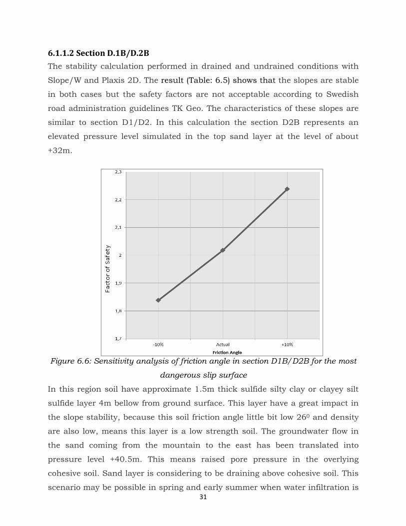
6.1.1.2 Section D.1B/D.2B The stability calculation performed in drained and undrained conditions with

Slope/W and Plaxis 2D. The result (Table: 6.5) shows that the slopes are stable

in both cases but the safety factors are not acceptable according to Swedish

road administration guidelines TK Geo. The characteristics of these slopes are

similar to section D1/D2. In this calculation the section D2B represents an

elevated pressure level simulated in the top sand layer at the level of about

+32m.

Figure 6.6: Sensitivity analysis of friction angle in section D1B/D2B for the most

dangerous slip surface

In this region soil have approximate 1.5m thick sulfide silty clay or clayey silt

sulfide layer 4m bellow from ground surface. This layer have a great impact in

the slope stability, because this soil friction angle little bit low 260 and density

are also low, means this layer is a low strength soil. The groundwater flow in

the sand coming from the mountain to the east has been translated into

pressure level +40.5m. This means raised pore pressure in the overlying

cohesive soil. Sand layer is considering to be draining above cohesive soil. This

scenario may be possible in spring and early summer when water infiltration is

32

Material "1 FillMaterial": PhiMaterial "2 saSi":PhiMaterial "3 MSa":PhiMaterial "4 saSi":PhiMaterial "5 SusiCl":PhiMaterial "6 Sa": PhiMaterial "7 Si": PhiMaterial "8 siMSa":Phi

Fac

tor

of S

afet

y

Sensitivity Range

0.45

0.5

0.55

0.6

0.65

0.7

0 0.2 0.4 0.6 0.8 1

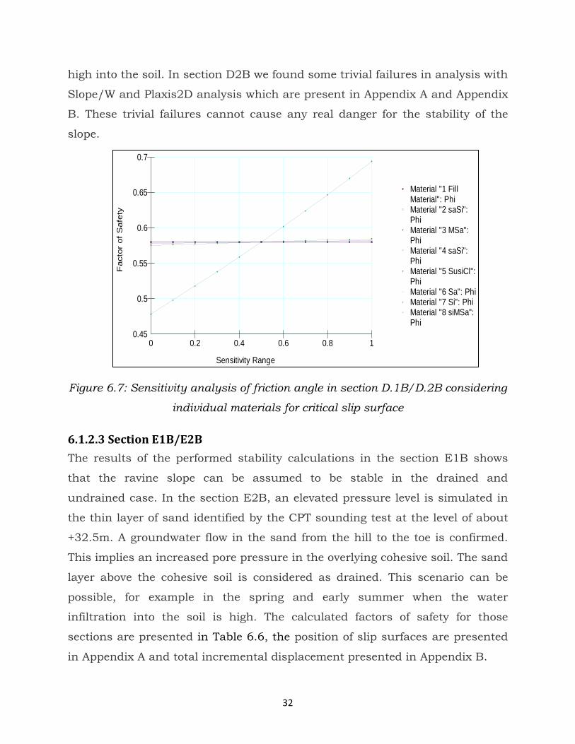
high into the soil. In section D2B we found some trivial failures in analysis with

Slope/W and Plaxis2D analysis which are present in Appendix A and Appendix

B. These trivial failures cannot cause any real danger for the stability of the

slope.

Figure 6.7: Sensitivity analysis of friction angle in section D.1B/D.2B considering

individual materials for critical slip surface

6.1.2.3 Section E1B/E2B The results of the performed stability calculations in the section E1B shows

that the ravine slope can be assumed to be stable in the drained and

undrained case. In the section E2B, an elevated pressure level is simulated in

the thin layer of sand identified by the CPT sounding test at the level of about

+32.5m. A groundwater flow in the sand from the hill to the toe is confirmed.

This implies an increased pore pressure in the overlying cohesive soil. The sand

layer above the cohesive soil is considered as drained. This scenario can be

possible, for example in the spring and early summer when the water

infiltration into the soil is high. The calculated factors of safety for those

sections are presented in Table 6.6, the position of slip surfaces are presented

in Appendix A and total incremental displacement presented in Appendix B.

33

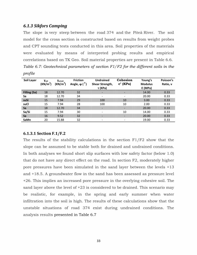
6.1.3 Sikfors Camping The slope is very steep between the road 374 and the Piteå River. The soil

model for the cross section is constructed based on results from weight probes

and CPT sounding tests conducted in this area. Soil properties of the materials

were evaluated by means of interpreted probing results and empirical

correlations based on TK Geo. Soil material properties are present in Table 6.6.

Table 6.7: Geotechnical parameters of section F1/F2 for the different soils in the

profile

Soil Layer ɣsat (KN/m3)

ɣunsat (KN/m3)

Friction Angle, φ ( 0 )

Undrained Shear Strength,

τ (KPa)

Cohesion c’ (KPa)

Young’s Modulus E (MPa)

Poisson’s Ratio, ν

Filling (Sa) 18 12.70 32 - - 14.00 0.33 Sa 18 12.70 34 - - 20.00 0.33 suSi 15 7.94 29 100 10 3.00 0.33 suCl 15 7.94 28 100 10 2.00 0.33 Sa 18 12.70 34 - - 20.00 0.33 Sa/Si 15 7.94 30 - 10 14.00 0.33 Sa 16 9.52 32 - - 20.00 0.33 SaMn 20 15.88 32 - - 19.00 0.33

6.1.3.1 Section F.1/F.2 The results of the stability calculations in the section F1/F2 show that the

slope can be assumed to be stable both for drained and undrained conditions.

In both analyses we found short slip surfaces with low safety factor (below 1.0)

that do not have any direct effect on the road. In section F2, moderately higher

pore pressures have been simulated in the sand layer between the levels +13

and +18.5. A groundwater flow in the sand has been assessed as pressure level

+26. This implies an increased pore pressure in the overlying cohesive soil. The

sand layer above the level of +23 is considered to be drained. This scenario may

be realistic, for example, in the spring and early summer when water

infiltration into the soil is high. The results of these calculations show that the

unstable situations of road 374 exist during undrained conditions. The

analysis results presented in Table 6.7

34

Table 6.8: Safety factor for Sikfors Camping

SectionName

Slope/W Plaxis 2D TyrensAnalysis TK Geo Allowable D* UD* D* UD* D* C* UD* C*

F1 0.94/1.74 1.49/1.72 0.93 0.98/1.18 1.68 1.36/0.76 1.5 1.3 F2 0.67/1.36 0.87/1.18 0.51 0.59 1.20 1.17/0.30 1.5 1.3 *D = Drained, *UN = Undrained and *C = Combined Analysis

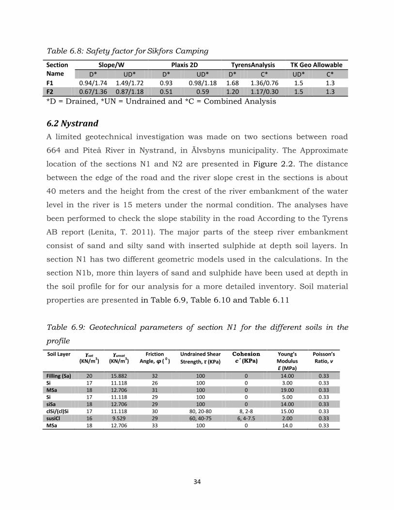
6.2 Nystrand A limited geotechnical investigation was made on two sections between road

664 and Piteå River in Nystrand, in Älvsbyns municipality. The Approximate

location of the sections N1 and N2 are presented in Figure 2.2. The distance

between the edge of the road and the river slope crest in the sections is about

40 meters and the height from the crest of the river embankment of the water

level in the river is 15 meters under the normal condition. The analyses have

been performed to check the slope stability in the road According to the Tyrens

AB report (Lenita, T. 2011). The major parts of the steep river embankment

consist of sand and silty sand with inserted sulphide at depth soil layers. In

section N1 has two different geometric models used in the calculations. In the

section N1b, more thin layers of sand and sulphide have been used at depth in

the soil profile for for our analysis for a more detailed inventory. Soil material

properties are presented in Table 6.9, Table 6.10 and Table 6.11

Table 6.9: Geotechnical parameters of section N1 for the different soils in the

profile Soil Layer ɣsat

(KN/m3) ɣunsat

(KN/m3) Friction

Angle, φ ( 0 ) Undrained Shear Strength, τ (KPa)

Cohesion c´ (KPa)

Young’s Modulus E (MPa)

Poisson’s Ratio, ν

Filling (Sa) 20 15.882 32 100 0 14.00 0.33 Si 17 11.118 26 100 0 3.00 0.33 MSa 18 12.706 31 100 0 19.00 0.33 Si 17 11.118 29 100 0 5.00 0.33 siSa 18 12.706 29 100 0 14.00 0.33 clSi/(cl)Si 17 11.118 30 80, 20-80 8, 2-8 15.00 0.33 susiCl 16 9.529 29 60, 40-75 6, 4-7.5 2.00 0.33 MSa 18 12.706 33 100 0 14.0 0.33

35

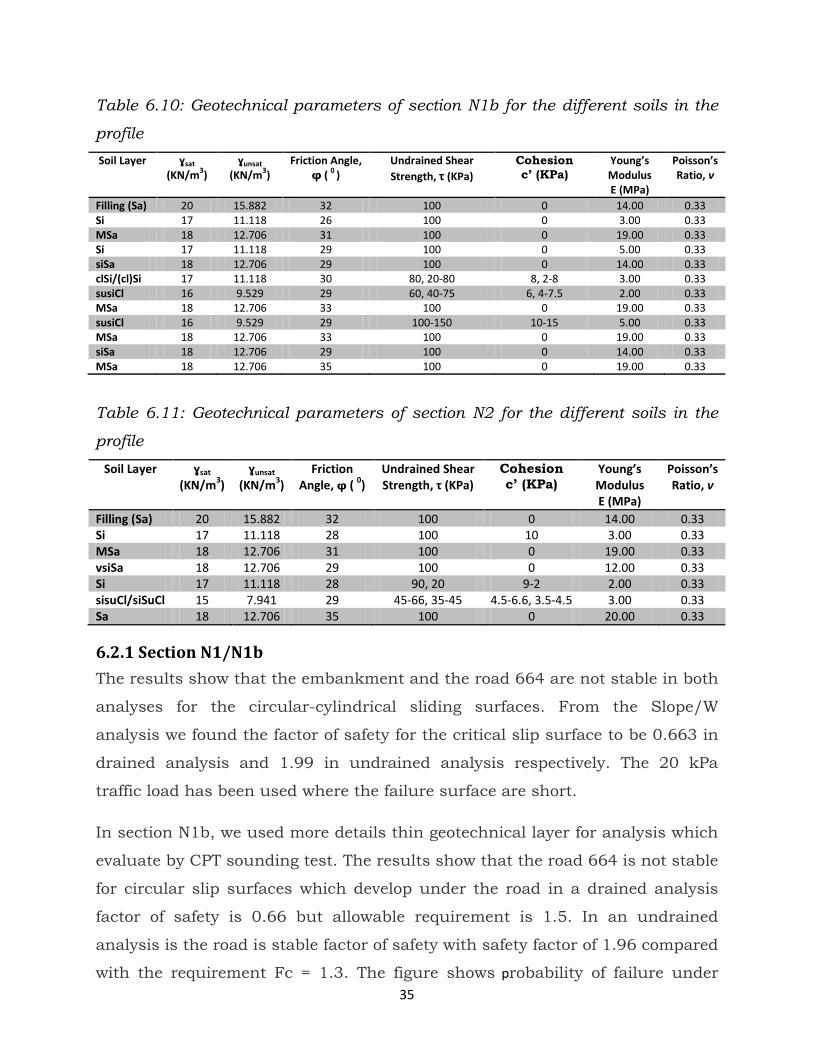
Table 6.10: Geotechnical parameters of section N1b for the different soils in the

profile Soil Layer ɣsat

(KN/m3) ɣunsat

(KN/m3) Friction Angle,

φ ( 0 ) Undrained Shear Strength, τ (KPa)

Cohesion c’ (KPa)

Young’s Modulus E (MPa)

Poisson’s Ratio, ν

Filling (Sa) 20 15.882 32 100 0 14.00 0.33 Si 17 11.118 26 100 0 3.00 0.33 MSa 18 12.706 31 100 0 19.00 0.33 Si 17 11.118 29 100 0 5.00 0.33 siSa 18 12.706 29 100 0 14.00 0.33 clSi/(cl)Si 17 11.118 30 80, 20-80 8, 2-8 3.00 0.33 susiCl 16 9.529 29 60, 40-75 6, 4-7.5 2.00 0.33 MSa 18 12.706 33 100 0 19.00 0.33 susiCl 16 9.529 29 100-150 10-15 5.00 0.33 MSa 18 12.706 33 100 0 19.00 0.33 siSa 18 12.706 29 100 0 14.00 0.33 MSa 18 12.706 35 100 0 19.00 0.33

Table 6.11: Geotechnical parameters of section N2 for the different soils in the

profile

Soil Layer ɣsat (KN/m3)

ɣunsat (KN/m3)

Friction Angle, φ ( 0)

Undrained Shear Strength, τ (KPa)

Cohesion c’ (KPa)

Young’s Modulus E (MPa)

Poisson’s Ratio, ν

Filling (Sa) 20 15.882 32 100 0 14.00 0.33 Si 17 11.118 28 100 10 3.00 0.33 MSa 18 12.706 31 100 0 19.00 0.33 vsiSa 18 12.706 29 100 0 12.00 0.33 Si 17 11.118 28 90, 20 9-2 2.00 0.33 sisuCl/siSuCl 15 7.941 29 45-66, 35-45 4.5-6.6, 3.5-4.5 3.00 0.33 Sa 18 12.706 35 100 0 20.00 0.33

6.2.1 Section N1/N1b The results show that the embankment and the road 664 are not stable in both

analyses for the circular-cylindrical sliding surfaces. From the Slope/W

analysis we found the factor of safety for the critical slip surface to be 0.663 in

drained analysis and 1.99 in undrained analysis respectively. The 20 kPa

traffic load has been used where the failure surface are short.

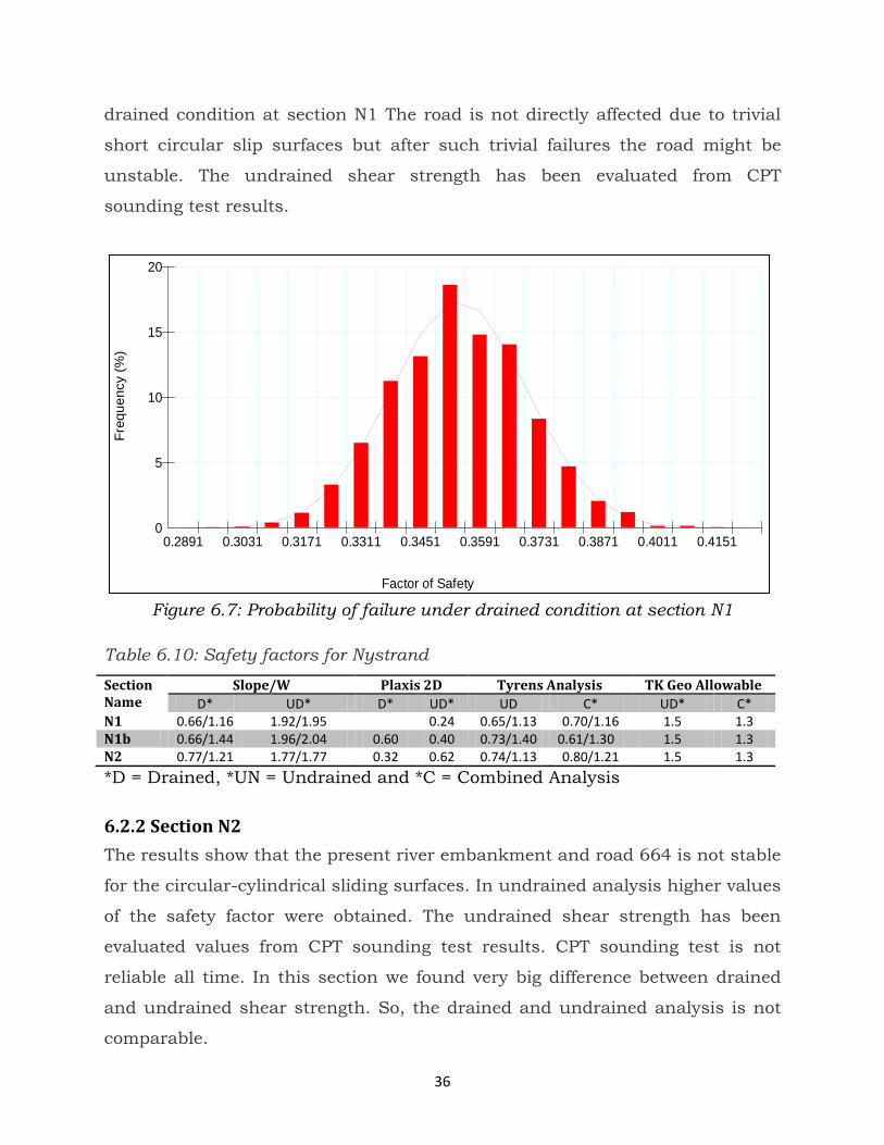
In section N1b, we used more details thin geotechnical layer for analysis which

evaluate by CPT sounding test. The results show that the road 664 is not stable

for circular slip surfaces which develop under the road in a drained analysis

factor of safety is 0.66 but allowable requirement is 1.5. In an undrained

analysis is the road is stable factor of safety with safety factor of 1.96 compared

with the requirement Fc = 1.3. The figure shows probability of failure under

36

Freq

uenc

y (%

)

Factor of Safety

0

5

10

15

20

0.2891 0.3031 0.3171 0.3311 0.3451 0.3591 0.3731 0.3871 0.4011 0.4151

drained condition at section N1 The road is not directly affected due to trivial

short circular slip surfaces but after such trivial failures the road might be

unstable. The undrained shear strength has been evaluated from CPT

sounding test results.

Figure 6.7: Probability of failure under drained condition at section N1

Table 6.10: Safety factors for Nystrand

Section Name

Slope/W Plaxis 2D Tyrens Analysis TK Geo Allowable D* UD* D* UD* UD C* UD* C*

N1 0.66/1.16 1.92/1.95 0.24 0.65/1.13 0.70/1.16 1.5 1.3 N1b 0.66/1.44 1.96/2.04 0.60 0.40 0.73/1.40 0.61/1.30 1.5 1.3 N2 0.77/1.21 1.77/1.77 0.32 0.62 0.74/1.13 0.80/1.21 1.5 1.3 *D = Drained, *UN = Undrained and *C = Combined Analysis

6.2.2 Section N2 The results show that the present river embankment and road 664 is not stable

for the circular-cylindrical sliding surfaces. In undrained analysis higher values

of the safety factor were obtained. The undrained shear strength has been

evaluated values from CPT sounding test results. CPT sounding test is not

reliable all time. In this section we found very big difference between drained

and undrained shear strength. So, the drained and undrained analysis is not

comparable.

37

7 CONCLUSIONS

Natural slope instability is a major concern in the area of Sikfors and Nystrand

where failures might cause catastrophic destruction on the surrounding area.

The failures might be triggered by internal or external factors that cause

imbalance to natural forces. An internal triggering factor is the factor that

causes failure due to internal changes, such as increasing pore water pressure

and or imbalanced forces developed due to external load.

Plaxis 2D is not good enough for natural slope stability analysis due to trivial

failures and can not indicate exact slip surface location. On the other hand,

with Slope/W it is easy to find out the position of the critical slip surface, safety

map, probabilistic failure and exact factor of safety. The factor of safety

computed from both Slope/W and Plaxis 2D decreases as the slope angle

becomes larger. The Limit equilibrium method overestimated the factor of

safety as compared to the Finite element method.

A distinction should be made between drained and undrained strength of

cohesive materials. As cohesive materials or clays generally possess less

permeability compared to sand, thus, the movement of water is restricted

whenever the soil is located. So, for clay, it might take years to dissipate the

excess pore water pressure before the effective equilibrium is reached. Shortly,

drained condition refers to the condition where drainage is allowed, while

undrained condition refers to the condition where drainage is restricted.

Sensitivity analyses performed indicate that an increase in the friction angle

and in the cohesion increases the factor of safety. Therefore the stability

analysis is much more sensitive to changes in friction angle and cohesion than

the unit weight of the layers. It was found that CPT sounding test result were

not reliable all the time. Trivial failures do not directly influence the stability of

the road but might progressively lead to failure. Results from this study

indicates that Nystrand and Sikfors Stora are critical places from a slope

stability point of view. Safety factors below the allowable limit have been

obtained on these places.

38

39

8 REFERENCES

a) Bishop, A. (1955). The Use of the Slip Circle in the Stability Analysis of Slope. Geotechnique, Vol. 5 (No. 1), pp. 7-17.

b) Fellenius, W. (1936). Calculation of Stability of Earth Dams. Transactions, 2nd Congress Large Dams, Vol. 4, p. 445. Washington D.C. New York: John Wiley and Sons Inc.

c) Lambe, T. and Whitmen, R. (1969). Soil Mechanics. New York: John Wiley and Sons Inc.

d) Mitchell R.A and Mitchell J.K. (1992). Stability Evaluation of Waste Landfills. Stability and Performance of Slope and Embankments-II (pp. 1152-1187). Berkeley, CA: 31 American Societies of Civil Engineers.

e) Morgenstern, N., & Price, V. (1965). The Analysis of the Stability of General Slip Surfaces. Geotechnique, Vol. 15 (No. 1), pp. 77-93.

f) Murthy, V. (1998). Geotechnical Engineering -Principles and Practices of Soil Mechanics and Foundation. New York: Marcel Dekker.

g) Whitman, R., & Bailey, W. (1967). Use of Computers for Slope Stability Analysis. Journal of the Soil Mechanics and Foundation Division, Vol. (Placeholder 3)

h) [Online citation: Date 21 February 2012.] http://www.dur.ac.uk/~des0www4/cal/slopes/page5.htm.

i) Lee W., Thomas S., Sunil S., and Glenn M.. 2002. Slope Stability and Stabilization Methods. 2nd Edition . New York : John Wiley & Sons, (2002). ISBN 0-471-38493-3.

j) Tornéus, L. (2011). Skredriskområden i BD-län Piteå älv. Luleå, Sweden : TYRENS AB, 2011

k) Stephen M., Wright G. (2005). Soil Strength and Slope

l) Chowdury, R.N. (1978). Slope Analysis. Amsterdam : Elsevier Scientific Publishing Company, 1978. ISBN 0-444-41662-5.

m) Knappett J., R.F. Craig. (2012). Soil Mechanics. New York: CRC Press Inc, 2012.

n) GEO-SLOPE International Ltd., Fourth Edition, November 2008

40

o) Waterman, D., Chesaru, A., Bonnier, P.G. and Galavi, V., Plaxis 2D 2010. Plaxis bv: Delft, Netherlands

p) Swedish Road Administration Guideline (TK Geo 11)

41

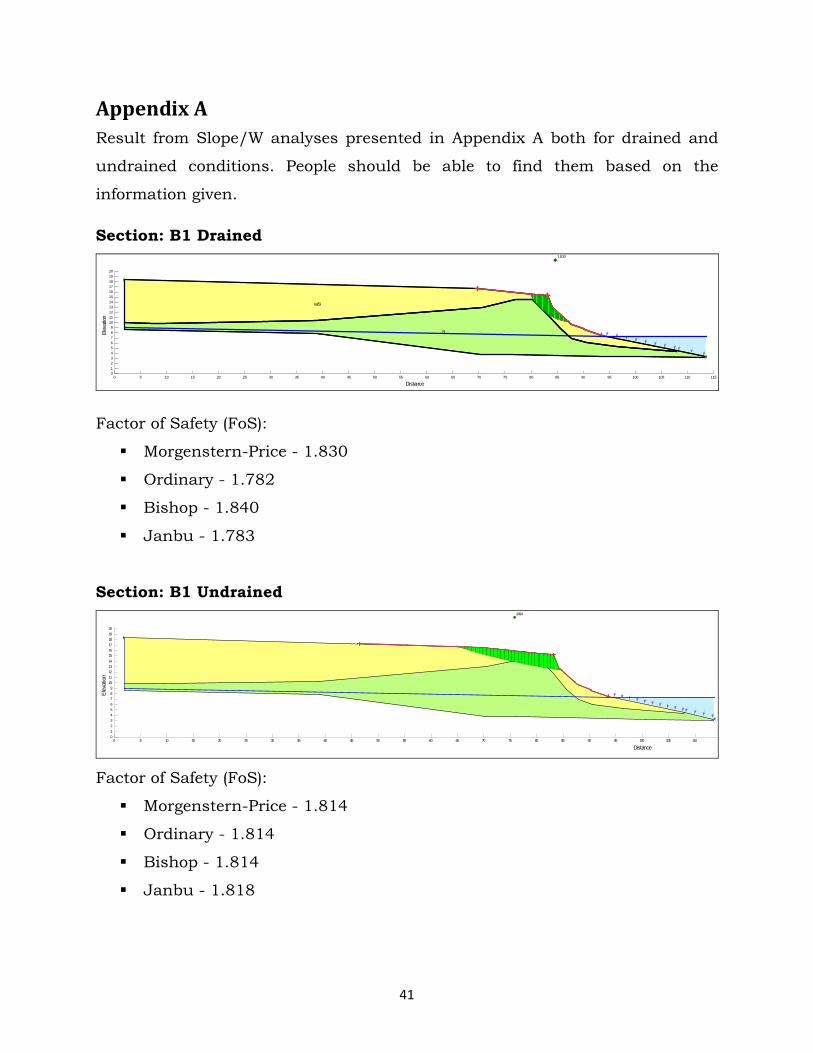
Appendix A Result from Slope/W analyses presented in Appendix A both for drained and

undrained conditions. People should be able to find them based on the

information given.

Section: B1 Drained

saSi

Si

1.830

Distance0 5 10 15 20 25 30 35 40 45 50 55 60 65 70 75 80 85 90 95 100 105 110 115

Elev

atio

n

0123456789

1011121314151617181920

Factor of Safety (FoS):

Morgenstern-Price - 1.830

Ordinary - 1.782

Bishop - 1.840

Janbu - 1.783

Section: B1 Undrained 1.814

Distance0 5 10 15 20 25 30 35 40 45 50 55 60 65 70 75 80 85 90 95 100 105 110

Elev

atio

n

0123456789

1011121314151617181920

Factor of Safety (FoS):

Morgenstern-Price - 1.814

Ordinary - 1.814

Bishop - 1.814

Janbu - 1.818

42

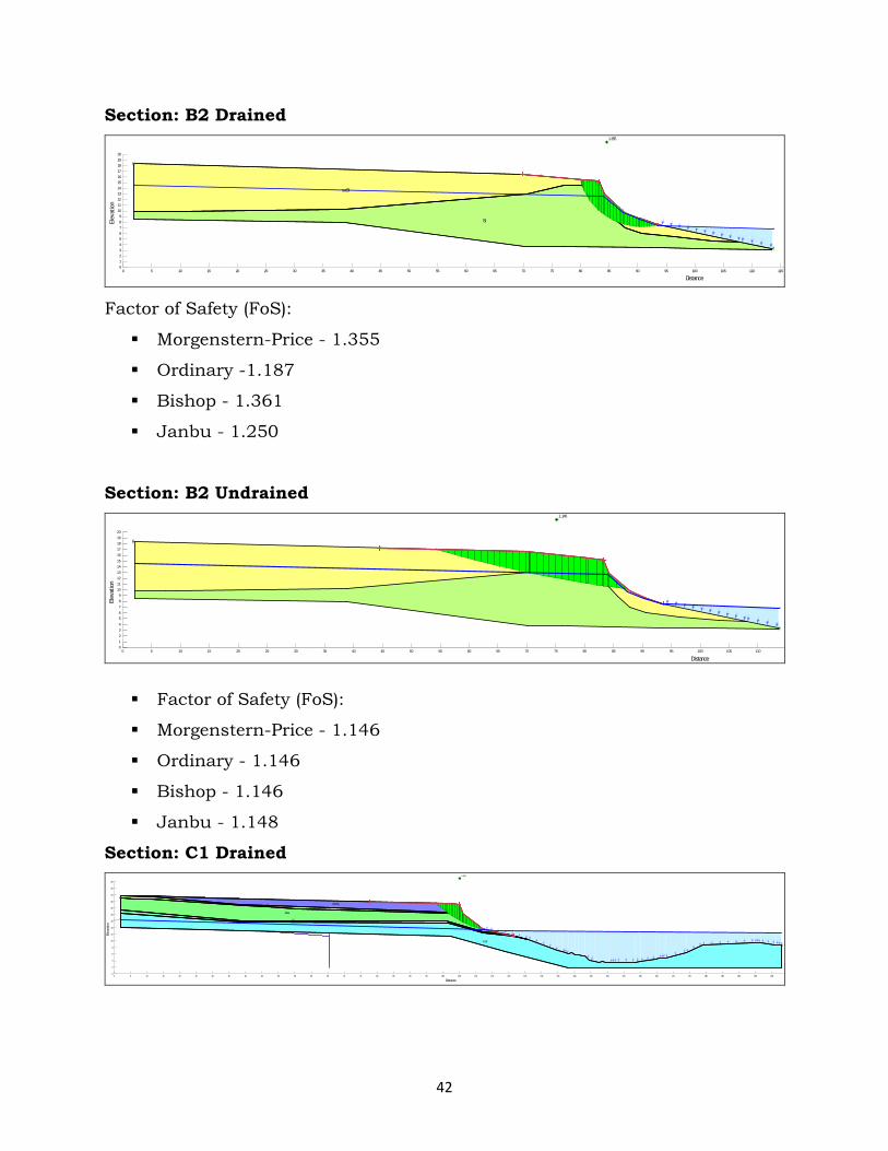
Section: B2 Drained

saSi

Si

1.355

Distance0 5 10 15 20 25 30 35 40 45 50 55 60 65 70 75 80 85 90 95 100 105 110 115

Elev

atio

n

0123456789

1011121314151617181920

Factor of Safety (FoS):

Morgenstern-Price - 1.355

Ordinary -1.187

Bishop - 1.361

Janbu - 1.250

Section: B2 Undrained 1.146

Distance0 5 10 15 20 25 30 35 40 45 50 55 60 65 70 75 80 85 90 95 100 105 110 1

Elev

ation

0123456789

1011121314151617181920

Factor of Safety (FoS):

Morgenstern-Price - 1.146

Ordinary - 1.146

Bishop - 1.146

Janbu - 1.148

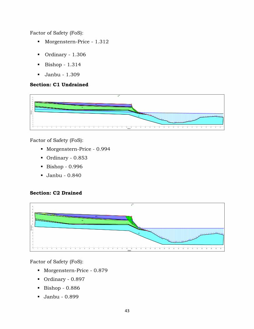
Section: C1 Drained

(Sa/Si)Si

MSa

Cl

saSi

1.312

Distance0 5 10 15 20 25 30 35 40 45 50 55 60 65 70 75 80 85 90 95 100 105 110 115 120 125 130 135 140 145 150 155 160 165 170 175 180 185 190 195 200

Elev

ation

0

2

4

6

8

10

12

14

16

18

20

22

24

26

28

43

Factor of Safety (FoS):

Morgenstern-Price - 1.312

Ordinary - 1.306

Bishop - 1.314

Janbu - 1.309

Section: C1 Undrained

(Sa/Si)Si

MSa

Cl

saSi

0.994

Distance0 5 10 15 20 25 30 35 40 45 50 55 60 65 70 75 80 85 90 95 100 105 110 115 120 125 130 135 140 145 150 155 160 165 170 175 180 185 190 195 200

Elev

atio

n

0

2

4

6

8

10

12

14

16

18

20

22

24

26

28

Factor of Safety (FoS):

Morgenstern-Price - 0.994

Ordinary - 0.853

Bishop - 0.996

Janbu - 0.840

Section: C2 Drained

(Sa/Si)Si

MSa

Cl

saSi

0.879

Distance0 5 10 15 20 25 30 35 40 45 50 55 60 65 70 75 80 85 90 95 100 105 110 115 120 125 130 135 140 145 150 155 160 165 170 175 180 185 190 195 200

Ele

vation

0

2

4

6

8

10

12

14

16

18

20

22

24

26

28

Factor of Safety (FoS):

Morgenstern-Price - 0.879

Ordinary - 0.897

Bishop - 0.886

Janbu - 0.899

44

Section: C2 Undrained

(Sa/Si)Si

MSa

Cl

saSi

0.747

Distance0 5 10 15 20 25 30 35 40 45 50 55 60 65 70 75 80 85 90 95 100 105 110 115 120 125 130 135 140 145 150 155 160 165 170 175 180 185 190 195 200 205

Ele

vatio

n

0

2

4

6

8

10

12

14

16

18

20

22

24

26

28

Factor of Safety (FoS):

Morgenstern-Price - 0.747

Ordinary - 0.745

Bishop - 0.751

Janbu - 0.746

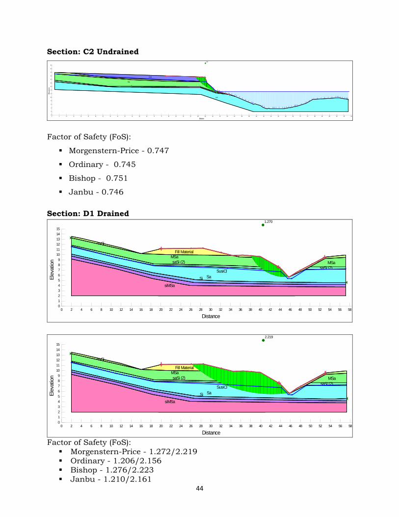
Section: D1 Drained

Fill Material

saSi

MSasaSi (2) saSi MSa

saSi (2)saSi

SusiClSaSi

siMSa

1.270

Distance0 2 4 6 8 10 12 14 16 18 20 22 24 26 28 30 32 34 36 38 40 42 44 46 48 50 52 54 56 58

Elev

atio

n

0123456789

101112131415

Fill Material

saSi

MSasaSi (2) saSi MSa

saSi (2)saSi

SusiClSaSi

siMSa

2.219

Distance0 2 4 6 8 10 12 14 16 18 20 22 24 26 28 30 32 34 36 38 40 42 44 46 48 50 52 54 56 58

Elev

atio

n

0123456789

101112131415

Factor of Safety (FoS): Morgenstern-Price - 1.272/2.219 Ordinary - 1.206/2.156 Bishop - 1.276/2.223 Janbu - 1.210/2.161

45

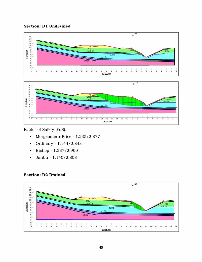
Section: D1 Undrained

Fill Material

saSi

MSasaSi (2) saSi MSa

saSi (2)saSi

SusiClSaSi

siMSa

1.235

Distance0 2 4 6 8 10 12 14 16 18 20 22 24 26 28 30 32 34 36 38 40 42 44 46 48 50 52 54 56 58

Elev

ation

0123456789

101112131415

Fill Material

saSi

MSasaSi (2) saSi MSa

saSi (2)saSi

SusiClSaSi

siMSa

2.877

Distance0 2 4 6 8 10 12 14 16 18 20 22 24 26 28 30 32 34 36 38 40 42 44 46 48 50 52 54 56 58

Eleva

tion

0123456789

101112131415

Factor of Safety (FoS):

Morgenstern-Price - 1.235/2.877

Ordinary - 1.144/2.843

Bishop - 1.237/2.900

Janbu - 1.140/2.808

Section: D2 Drained

Fill Material

saSi

MSasaSi (2) saSi MSa

saSi (2)

saSi

SusiClSaSi

siMSa

1.389

Distance0 2 4 6 8 10 12 14 16 18 20 22 24 26 28 30 32 34 36 38 40 42 44 46 48 50 52 54 56 58

Elev

atio

n

0123456789

101112131415

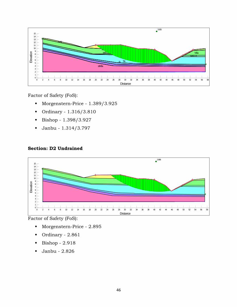
46

Fill Material

saSi

MSasaSi (2) saSi MSa

saSi (2)

saSi

SusiClSaSi

siMSa

3.925

Distance0 2 4 6 8 10 12 14 16 18 20 22 24 26 28 30 32 34 36 38 40 42 44 46 48 50 52 54 56 58

Elev

atio

n

0123456789

101112131415

Factor of Safety (FoS):

Morgenstern-Price - 1.389/3.925

Ordinary - 1.316/3.810

Bishop - 1.398/3.927

Janbu - 1.314/3.797

Section: D2 Undrained

2.895

Distance0 2 4 6 8 10 12 14 16 18 20 22 24 26 28 30 32 34 36 38 40 42 44 46 48 50 52 54 56 58

Elev

atio

n

0123456789

101112131415

Factor of Safety (FoS):

Morgenstern-Price - 2.895

Ordinary - 2.861

Bishop - 2.918

Janbu - 2.826

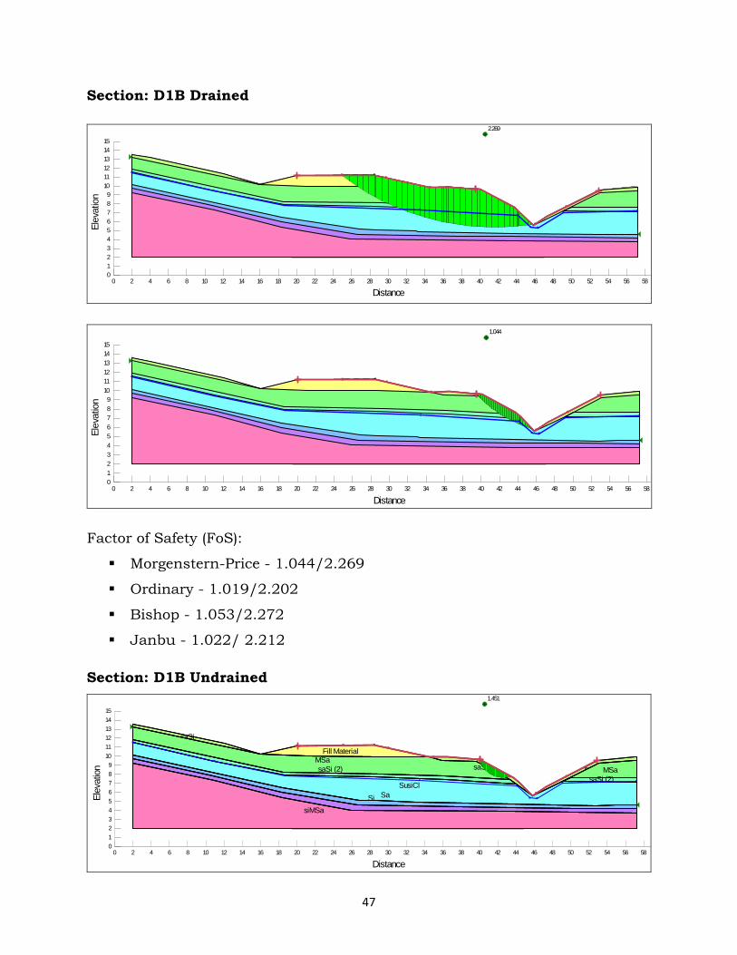
47

Section: D1B Drained

2.269

Distance0 2 4 6 8 10 12 14 16 18 20 22 24 26 28 30 32 34 36 38 40 42 44 46 48 50 52 54 56 58

Elev

atio

n

0123456789

101112131415

1.044

Distance0 2 4 6 8 10 12 14 16 18 20 22 24 26 28 30 32 34 36 38 40 42 44 46 48 50 52 54 56 58

Elev

atio

n

0123456789

101112131415

Factor of Safety (FoS):

Morgenstern-Price - 1.044/2.269

Ordinary - 1.019/2.202

Bishop - 1.053/2.272

Janbu - 1.022/ 2.212

Section: D1B Undrained

Fill Material

saSi

MSasaSi (2) saSi MSa

saSi (2)saSi

SusiClSaSi

siMSa

1.451

Distance0 2 4 6 8 10 12 14 16 18 20 22 24 26 28 30 32 34 36 38 40 42 44 46 48 50 52 54 56 58

Elev

atio

n

0123456789

101112131415

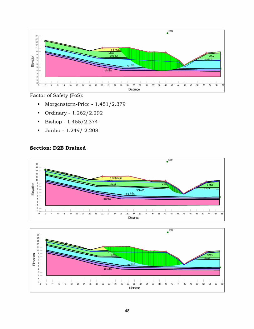
48

Fill Material

saSi

MSasaSi (2) saSi MSa

saSi (2)saSi

SusiClSaSi

siMSa

2.379

Distance0 2 4 6 8 10 12 14 16 18 20 22 24 26 28 30 32 34 36 38 40 42 44 46 48 50 52 54 56 58

Elev

atio

n

0123456789

101112131415

Factor of Safety (FoS):

Morgenstern-Price - 1.451/2.379

Ordinary - 1.262/2.292

Bishop - 1.455/2.374

Janbu - 1.249/ 2.208

Section: D2B Drained

1 Fill Material

2 saSi

3 MSa4 saSi 2 saSi 3 MSa

4 saSi2 saSi

5 SusiCl6 Sa7 Si

8 siMSa

0.580

Distance0 2 4 6 8 10 12 14 16 18 20 22 24 26 28 30 32 34 36 38 40 42 44 46 48 50 52 54 56 58

Elev

atio

n

0123456789

101112131415

1 Fill Material

2 saSi

3 MSa4 saSi 2 saSi 3 MSa

4 saSi2 saSi

5 SusiCl6 Sa7 Si

8 siMSa

2.028

Distance0 2 4 6 8 10 12 14 16 18 20 22 24 26 28 30 32 34 36 38 40 42 44 46 48 50 52 54 56 58

Elev

atio

n

0123456789

101112131415

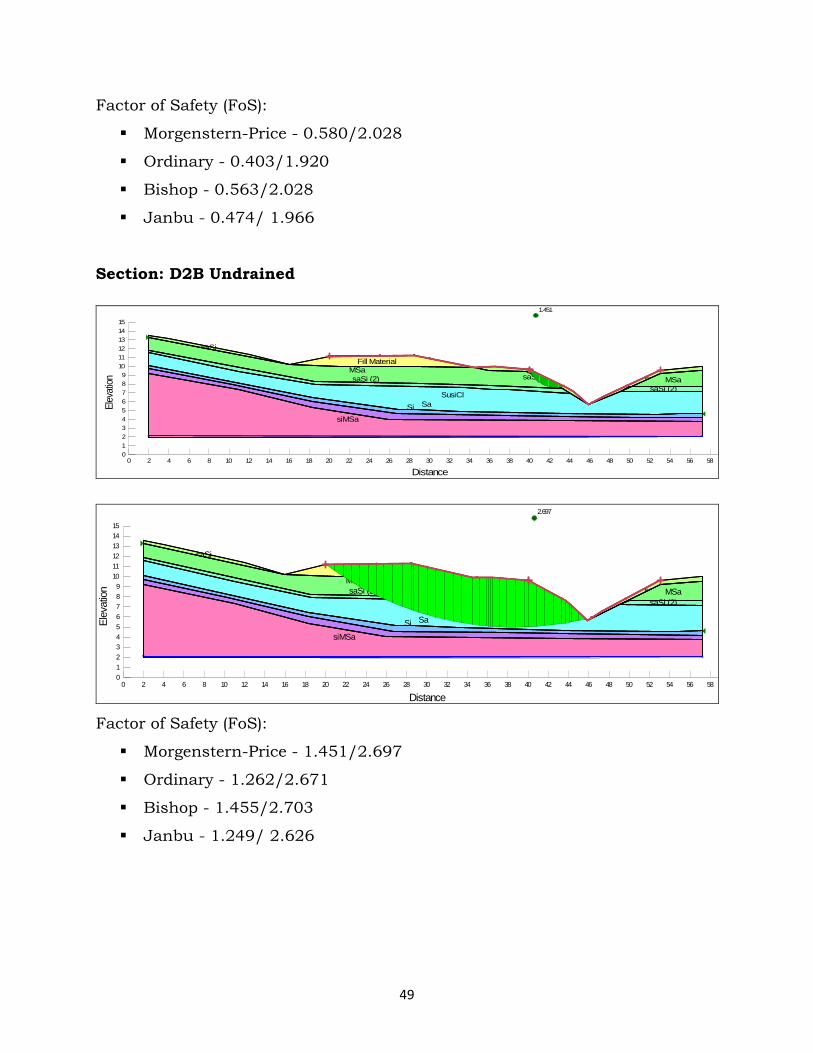
49

Factor of Safety (FoS):

Morgenstern-Price - 0.580/2.028

Ordinary - 0.403/1.920

Bishop - 0.563/2.028

Janbu - 0.474/ 1.966

Section: D2B Undrained

Fill Material

saSi

MSasaSi (2) saSi MSa

saSi (2)saSi

SusiClSaSi

siMSa

1.451

Distance0 2 4 6 8 10 12 14 16 18 20 22 24 26 28 30 32 34 36 38 40 42 44 46 48 50 52 54 56 58

Elev

ation

0123456789

101112131415

Fill Material

saSi

MSasaSi (2) saSi MSa

saSi (2)saSi

SusiClSaSi

siMSa

2.697

Distance0 2 4 6 8 10 12 14 16 18 20 22 24 26 28 30 32 34 36 38 40 42 44 46 48 50 52 54 56 58

Elev

atio

n

0123456789

101112131415

Factor of Safety (FoS):

Morgenstern-Price - 1.451/2.697

Ordinary - 1.262/2.671

Bishop - 1.455/2.703

Janbu - 1.249/ 2.626

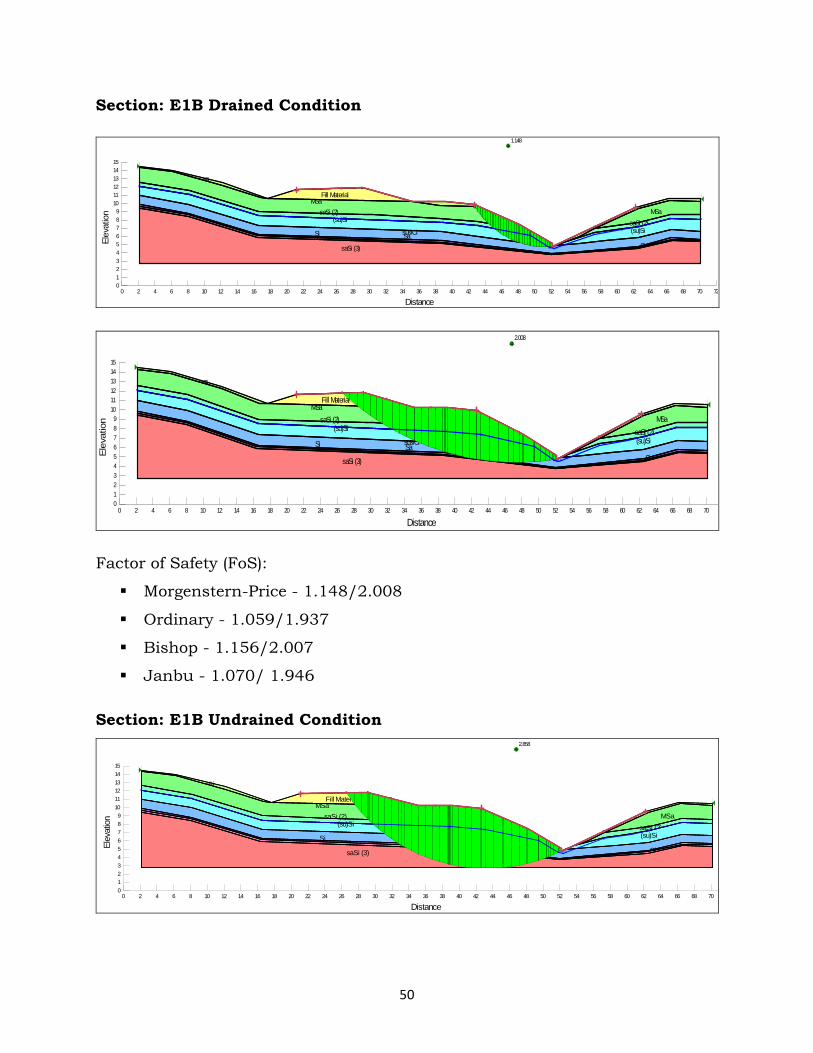
50

Section: E1B Drained Condition

saSi

MSasaSi (2)

Fill Material

saSi saSi MSasaSi (2)(su)Si

(su)Si

susiClSaSi

SisaSi (3)

1.148

Distance0 2 4 6 8 10 12 14 16 18 20 22 24 26 28 30 32 34 36 38 40 42 44 46 48 50 52 54 56 58 60 62 64 66 68 70 72

Elev

atio

n

0123456789

101112131415

saSi

MSasaSi (2)

Fill Material

saSi saSi MSasaSi (2)(su)Si

(su)Si

susiClSaSi

SisaSi (3)

2.008

Distance0 2 4 6 8 10 12 14 16 18 20 22 24 26 28 30 32 34 36 38 40 42 44 46 48 50 52 54 56 58 60 62 64 66 68 70

Ele

vatio

n

0123456789

101112131415

Factor of Safety (FoS):

Morgenstern-Price - 1.148/2.008

Ordinary - 1.059/1.937

Bishop - 1.156/2.007

Janbu - 1.070/ 1.946

Section: E1B Undrained Condition

saSi

MSasaSi (2)

Fill Material

saSi saSi MSasaSi (2)(su)Si

(su)Si

susiClSaSi

SisaSi (3)

2.858

Distance0 2 4 6 8 10 12 14 16 18 20 22 24 26 28 30 32 34 36 38 40 42 44 46 48 50 52 54 56 58 60 62 64 66 68 70

Elev

atio

n

0123456789

101112131415

51

Factor of Safety (FoS):

Morgenstern-Price - 2.858

Ordinary - 2.606

Bishop - 2.807

Janbu - 2.539

Section: E2B Drained Condition

saSi

MSasaSi (2)

Fill Material

saSi saSi MSasaSi (2)(su)Si

(su)Si

susiClSaSi

SisaSi (3)

2.604

Distance0 2 4 6 8 10 12 14 16 18 20 22 24 26 28 30 32 34 36 38 40 42 44 46 48 50 52 54 56 58 60 62 64 66 68 70

Elev

atio

n

0123456789

101112131415

Factor of Safety (FoS):

Morgenstern-Price - 2.604

Ordinary - 2.522

Bishop - 2.604

Janbu - 2.510

Section: E2B Undrained Condition

saSi

MSasaSi (2)

Fill Material

saSi saSi MSasaSi (2)(su)Si

(su)Si

susiClSaSi

SisaSi (3)

2.980

Distance0 2 4 6 8 10 12 14 16 18 20 22 24 26 28 30 32 34 36 38 40 42 44 46 48 50 52 54 56 58 60 62 64 66 68 70

Eleva

tion

0123456789

101112131415

Factor of Safety (FoS):

Morgenstern-Price - 2.980

Ordinary - 2.969

Bishop - 2.996

Janbu - 2.984

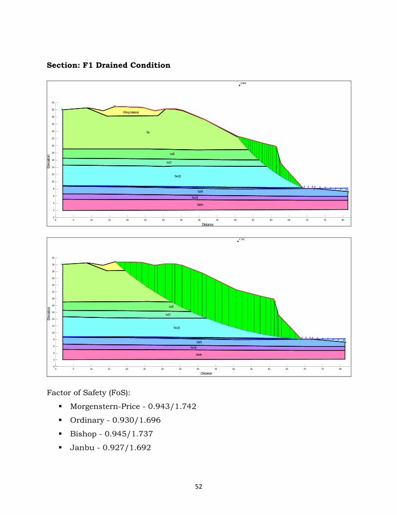
52

Section: F1 Drained Condition

Filling Material

Sa

suSi

suCl

Sa (2)

Sa (2)Sa/Si

Sa (3)

SaMn

0.943

Distance0 5 10 15 20 25 30 35 40 45 50 55 60 65 70 75 80

Elev

atio

n

0

2

4

6

8

10

12

14

16

18

20

22

24

26

28

30

32

Filling Material

Sa

suSi

suCl

Sa (2)

Sa (2)Sa/Si

Sa (3)

SaMn

1.742

Distance0 5 10 15 20 25 30 35 40 45 50 55 60 65 70 75 80

Elev

atio

n

0

2

4

6

8

10

12

14

16

18

20

22

24

26

28

30

32

Factor of Safety (FoS):

Morgenstern-Price - 0.943/1.742

Ordinary - 0.930/1.696

Bishop - 0.945/1.737

Janbu - 0.927/1.692

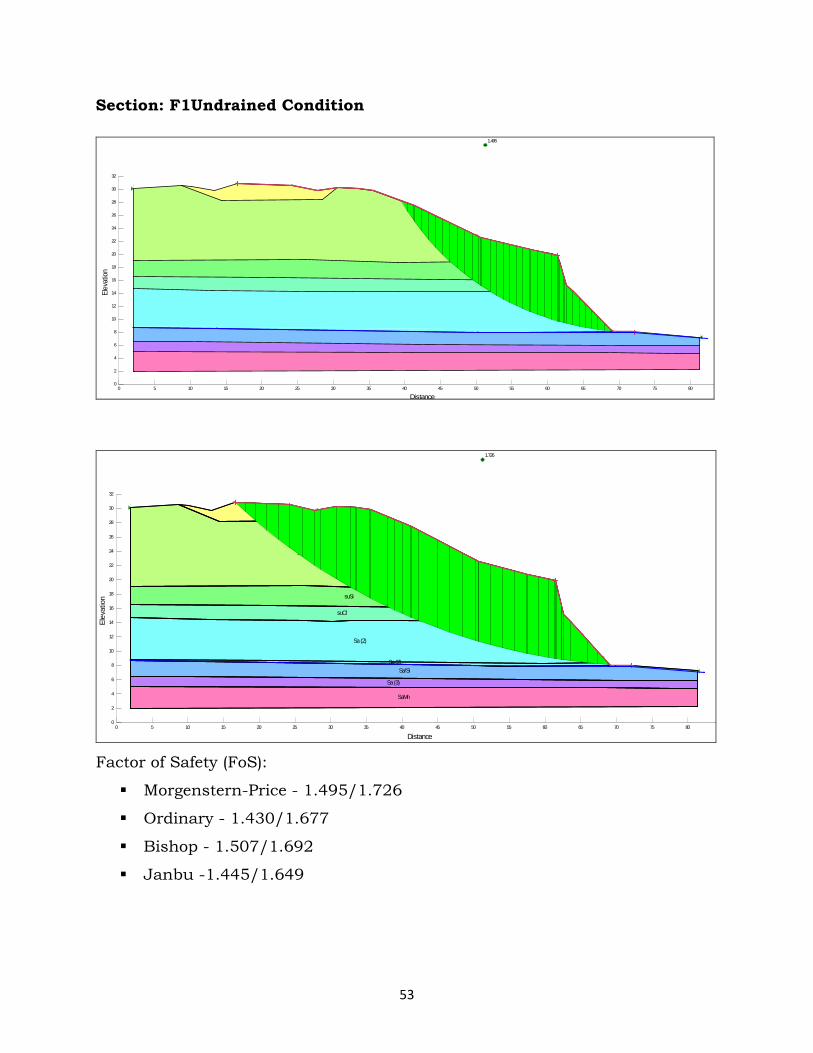
53

Section: F1Undrained Condition

1.495

Distance0 5 10 15 20 25 30 35 40 45 50 55 60 65 70 75 80

Elev

ation

0

2

4

6

8

10

12

14

16

18

20

22

24

26

28

30

32

Filling Material

Sa

suSi

suCl

Sa (2)

Sa (2)Sa/Si

Sa (3)

SaMn

1.726

Distance0 5 10 15 20 25 30 35 40 45 50 55 60 65 70 75 80

Elev

atio

n

0

2

4

6

8

10

12

14

16

18

20

22

24

26

28

30

32

Factor of Safety (FoS):

Morgenstern-Price - 1.495/1.726

Ordinary - 1.430/1.677

Bishop - 1.507/1.692

Janbu -1.445/1.649

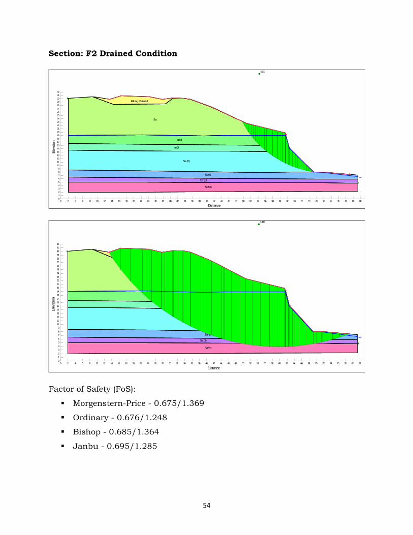
54

Section: F2 Drained Condition

Filling Material

Sa

suSi

suCl

Sa (2)

Sa/Si

Sa (3)

SaMn

0.675

Distance0 2 4 6 8 10 12 14 16 18 20 22 24 26 28 30 32 34 36 38 40 42 44 46 48 50 52 54 56 58 60 62 64 66 68 70 72 74 76 78 80 82

Elev

ation

0123456789

1011121314151617181920212223242526272829303132

Filling Material

Sa

suSi

suCl

Sa (2)

Sa/Si

Sa (3)

SaMn

1.369

Distance0 2 4 6 8 10 12 14 16 18 20 22 24 26 28 30 32 34 36 38 40 42 44 46 48 50 52 54 56 58 60 62 64 66 68 70 72 74 76 78 80 82

Elev

atio

n

0123456789

1011121314151617181920212223242526272829303132

Factor of Safety (FoS):

Morgenstern-Price - 0.675/1.369

Ordinary - 0.676/1.248

Bishop - 0.685/1.364

Janbu - 0.695/1.285

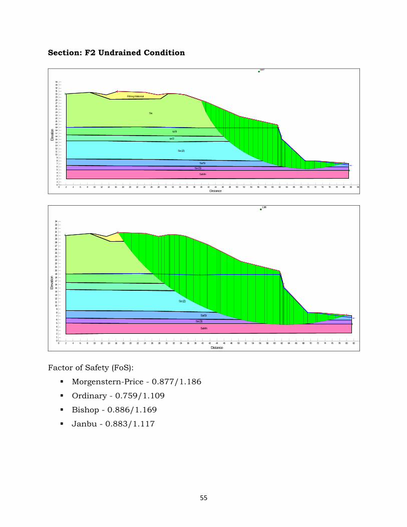
55

Section: F2 Undrained Condition

Filling Material

Sa

suSi

suCl

Sa (2)

Sa/Si

Sa (3)

SaMn

0.877

Distance0 2 4 6 8 10 12 14 16 18 20 22 24 26 28 30 32 34 36 38 40 42 44 46 48 50 52 54 56 58 60 62 64 66 68 70 72 74 76 78 80 82 84

Elev

ation

0123456789

10111213141516171819202122232425262728293031323334

Filling Material

Sa

suSi

suCl

Sa (2)

Sa/Si

Sa (3)

SaMn

1.186

Distance0 2 4 6 8 10 12 14 16 18 20 22 24 26 28 30 32 34 36 38 40 42 44 46 48 50 52 54 56 58 60 62 64 66 68 70 72 74 76 78 80 82

Elev

atio

n

0123456789

10111213141516171819202122232425262728293031323334

Factor of Safety (FoS):

Morgenstern-Price - 0.877/1.186

Ordinary - 0.759/1.109

Bishop - 0.886/1.169

Janbu - 0.883/1.117

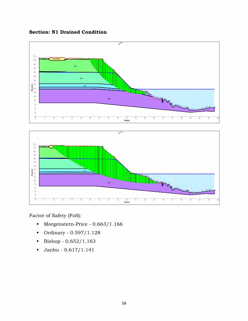
56

Section: N1 Drained Condition

Si Filling Material Si

Msa

Si (2)

siSa

clSi

susiCl

MSa

0.663

Distance0 5 10 15 20 25 30 35 40 45 50 55 60 65 70 75 80 85 90 95 100

Elev

atio

n

0

2

4

6

8

10

12

14

16

18

20

22

24

26

28

30

Si Filling Material Si

Msa

Si (2)

siSa

clSi

susiCl

MSa

1.166

Distance0 5 10 15 20 25 30 35 40 45 50 55 60 65 70 75 80 85 90 95 100

Elev

ation

0

2

4

6

8

10

12

14

16

18

20

22

24

26

28

30

Factor of Safety (FoS):

Morgenstern-Price - 0.663/1.166

Ordinary - 0.597/1.128

Bishop - 0.652/1.163

Janbu - 0.617/1.141

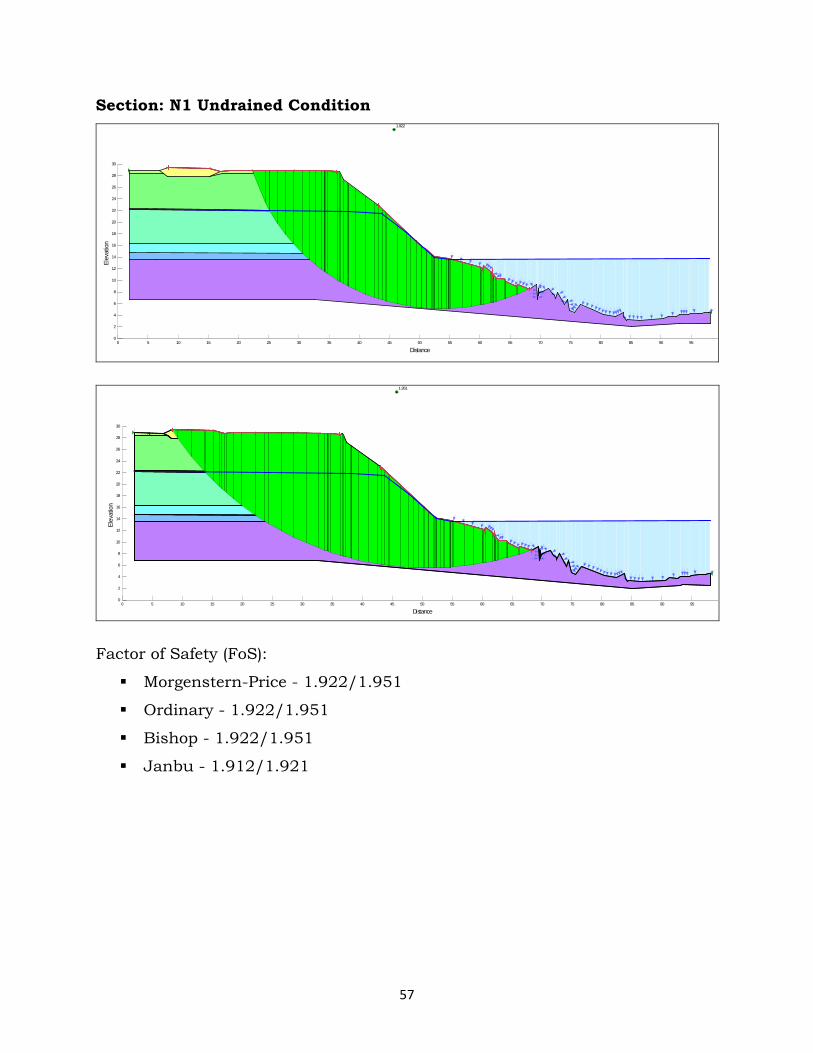
57

Section: N1 Undrained Condition 1.922

Distance0 5 10 15 20 25 30 35 40 45 50 55 60 65 70 75 80 85 90 95

Elev

atio

n

0

2

4

6

8

10

12

14

16

18

20

22

24

26

28

30

Si Filling Material Si

Msa

Si (2)

siSa

clSi

susiCl

MSa

1.951

Distance0 5 10 15 20 25 30 35 40 45 50 55 60 65 70 75 80 85 90 95

Elev

atio

n

0

2

4

6

8

10

12

14

16

18

20

22

24

26

28

30

Factor of Safety (FoS):

Morgenstern-Price - 1.922/1.951

Ordinary - 1.922/1.951

Bishop - 1.922/1.951

Janbu - 1.912/1.921

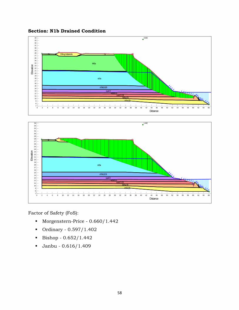
58

Section: N1b Drained Condition

Si Filling Materials Si

MSa

Si (2)

siSa

clSi/(cl)Si

susiClMSa (2)

susiCl (2)MSa (3)

siSa (2)

0.660

Distance0 2 4 6 8 10 12 14 16 18 20 22 24 26 28 30 32 34 36 38 40 42 44 46 48 50 52 54 56 58 60 62 64 66

Elev

atio

n

789

10111213141516171819202122232425262728293031323334

Si Filling Materials Si

MSa

Si (2)

siSa

clSi/(cl)Si

susiClMSa (2)

susiCl (2)MSa (3)

siSa (2)

1.442

Distance0 2 4 6 8 10 12 14 16 18 20 22 24 26 28 30 32 34 36 38 40 42 44 46 48 50 52 54 56 58 60 62 64 66

Elev

atio

n

789

10111213141516171819202122232425262728293031323334

Factor of Safety (FoS):

Morgenstern-Price - 0.660/1.442

Ordinary - 0.597/1.402

Bishop - 0.652/1.442

Janbu - 0.616/1.409

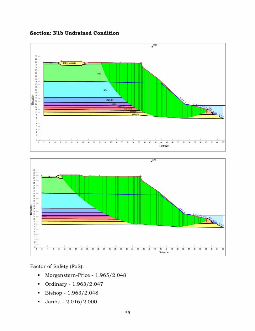
59

Section: N1b Undrained Condition

Si Filling Materials Si

MSa

Si (2)

siSa

clSi/(cl)SisusiCl

MSa (2)susiCl (2)

MSa (3)siSa (2)

1.965

Distance0 2 4 6 8 10 12 14 16 18 20 22 24 26 28 30 32 34 36 38 40 42 44 46 48 50 52 54 56 58 60 62 64 66

Elev

atio

n

0123456789

101112131415161718192021222324252627282930

Si Filling Materials Si

MSa

Si (2)

siSa

clSi/(cl)SisusiCl

MSa (2)susiCl (2)

MSa (3)siSa (2)

2.048

Distance0 2 4 6 8 10 12 14 16 18 20 22 24 26 28 30 32 34 36 38 40 42 44 46 48 50 52 54 56 58 60 62 64 66

Elev

ation

0123456789

101112131415161718192021222324252627282930

Factor of Safety (FoS):

Morgenstern-Price - 1.965/2.048

Ordinary - 1.963/2.047

Bishop - 1.963/2.048

Janbu - 2.016/2.000

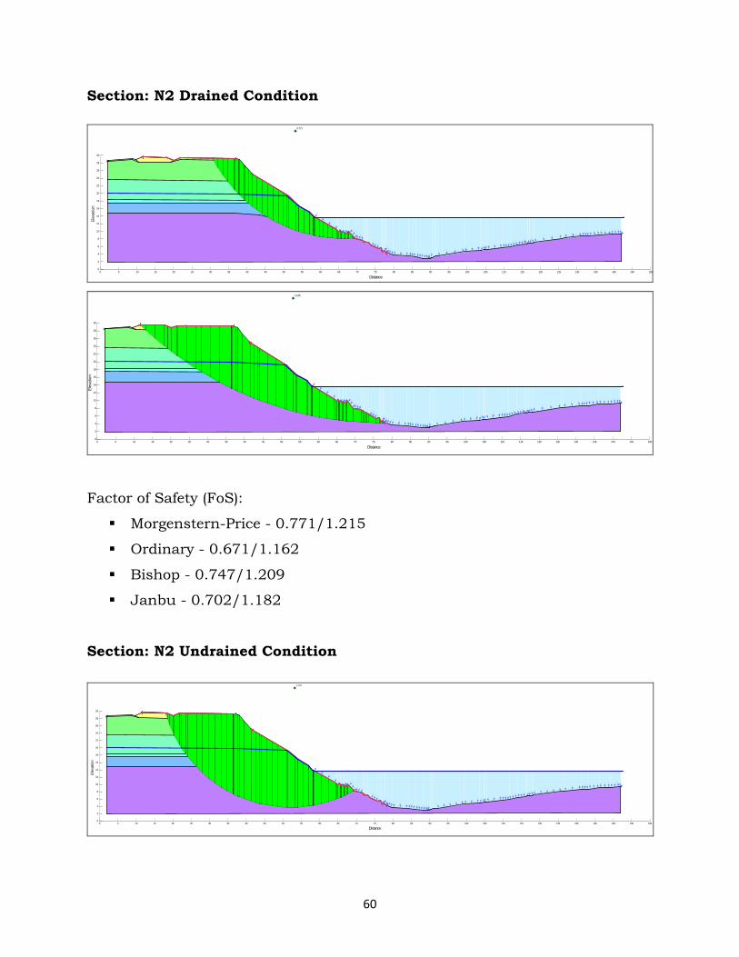
60

Section: N2 Drained Condition

0.771

Distance0 5 10 15 20 25 30 35 40 45 50 55 60 65 70 75 80 85 90 95 100 105 110 115 120 125 130 135 140 145 150

Elev

atio

n

0

2

4

6

8

10

12

14

16

18

20

22

24

26

28

30

1.215

Distance0 5 10 15 20 25 30 35 40 45 50 55 60 65 70 75 80 85 90 95 100 105 110 115 120 125 130 135 140 145 150

Elev

atio

n

0

2

4

6

8

10

12

14

16

18

20

22

24

26

28

30

Factor of Safety (FoS):

Morgenstern-Price - 0.771/1.215

Ordinary - 0.671/1.162

Bishop - 0.747/1.209

Janbu - 0.702/1.182

Section: N2 Undrained Condition

1.770

Distance0 5 10 15 20 25 30 35 40 45 50 55 60 65 70 75 80 85 90 95 100 105 110 115 120 125 130 135 140 145 150

Elev

atio

n

0

2

4

6

8

10

12

14

16

18

20

22

24

26

28

30

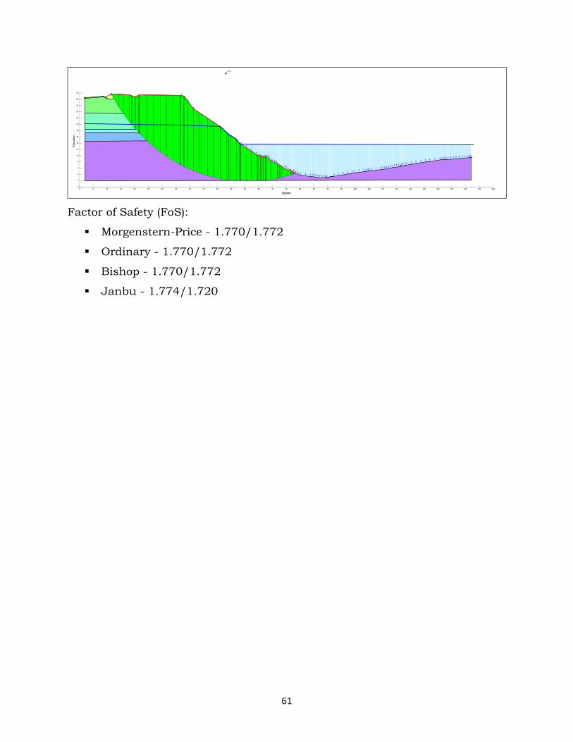
61

1.772

Distance0 5 10 15 20 25 30 35 40 45 50 55 60 65 70 75 80 85 90 95 100 105 110 115 120 125 130 135 140 145 150

Ele

vatio

n

0

2

4

6

8

10

12

14

16

18

20

22

24

26

28

30

Factor of Safety (FoS):

Morgenstern-Price - 1.770/1.772

Ordinary - 1.770/1.772

Bishop - 1.770/1.772

Janbu - 1.774/1.720

62

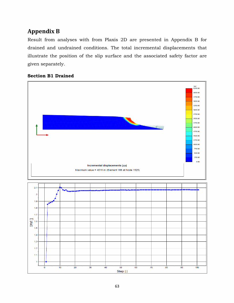
63

Appendix B Result from analyses with from Plaxis 2D are presented in Appendix B for

drained and undrained conditions. The total incremental displacements that

illustrate the position of the slip surface and the associated safety factor are

given separately.

Section B1 Drained

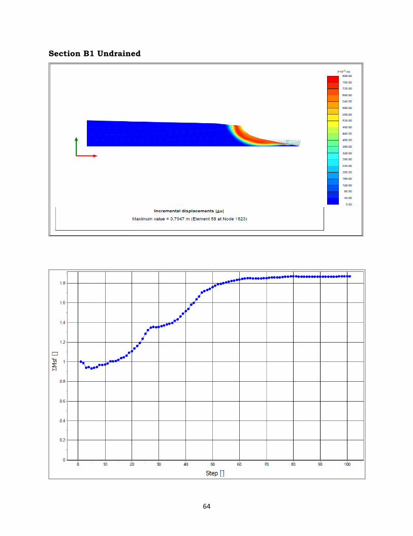
64

Section B1 Undrained

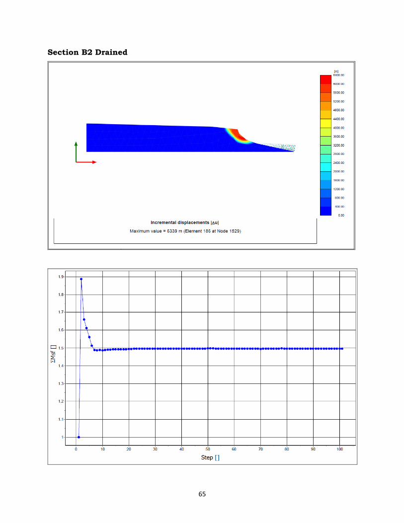
65

Section B2 Drained

66

Section B2 Undrained

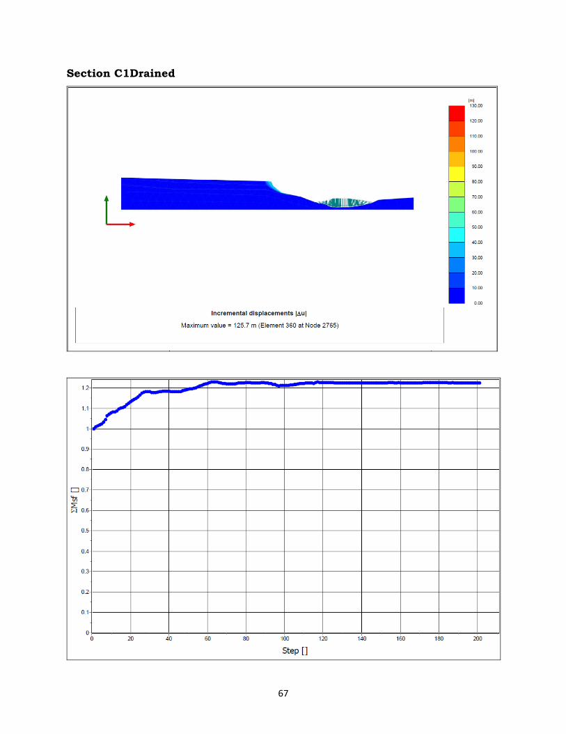
67

Section C1Drained

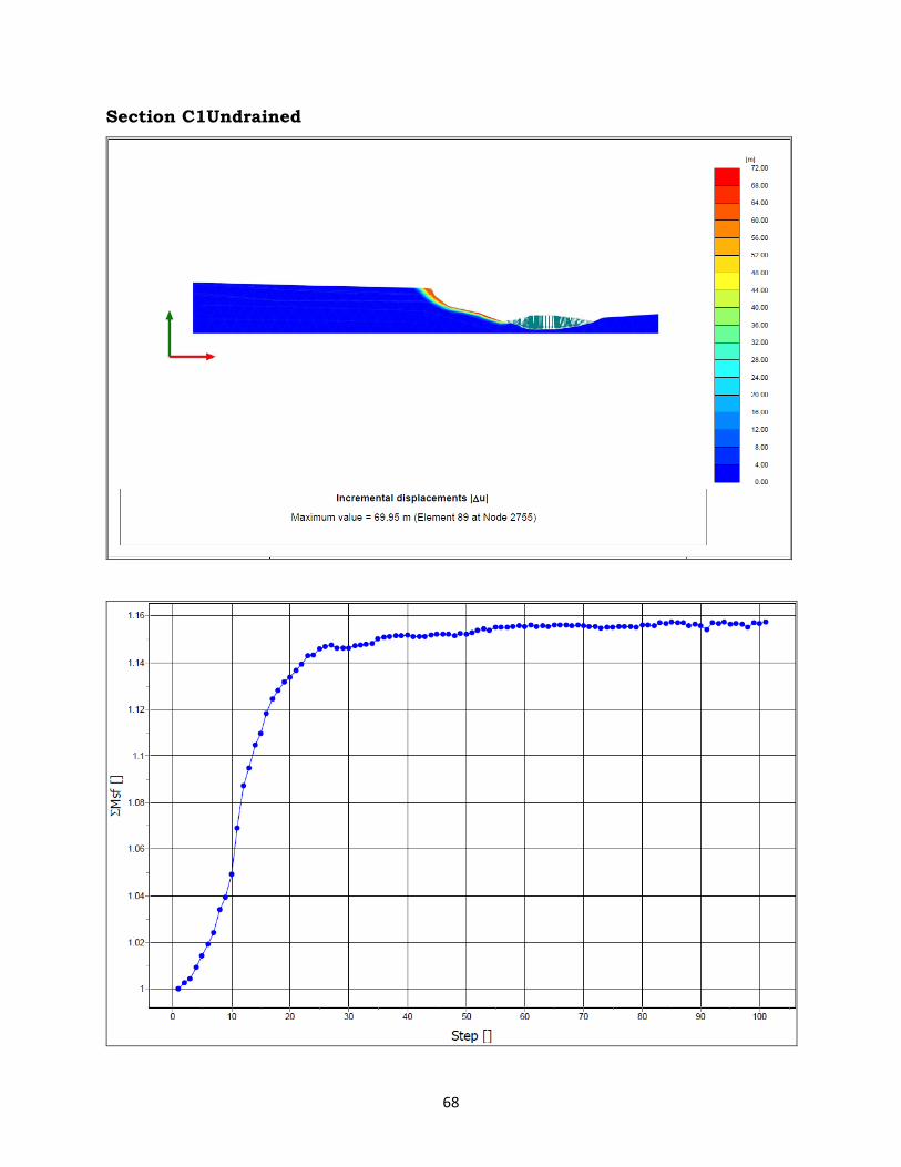
68

Section C1Undrained

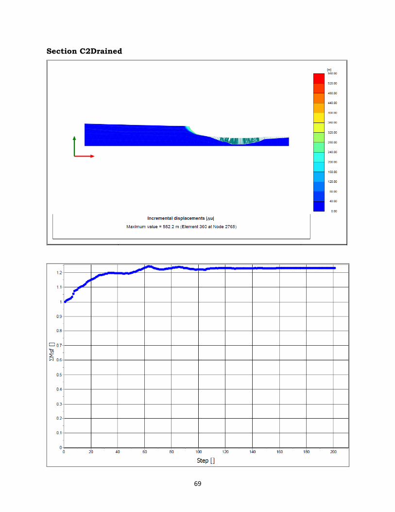
69

Section C2Drained

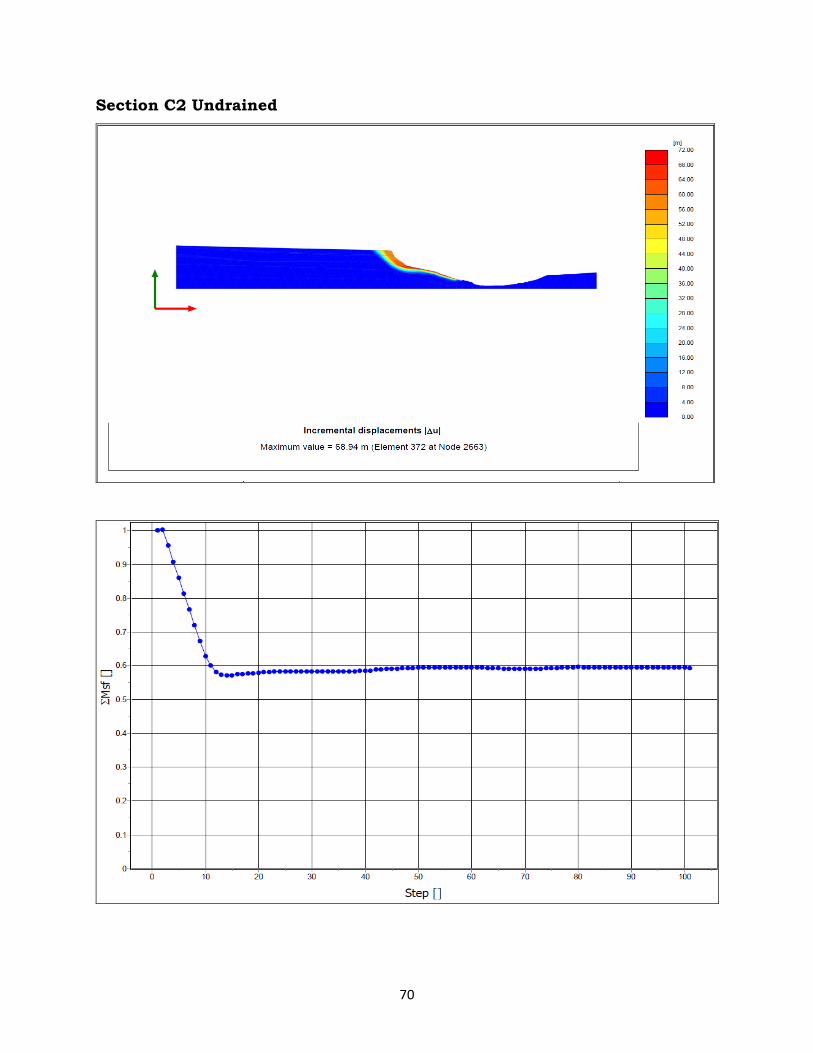
70

Section C2 Undrained

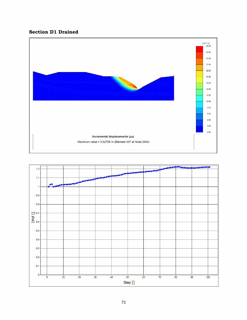
71

Section D1 Drained

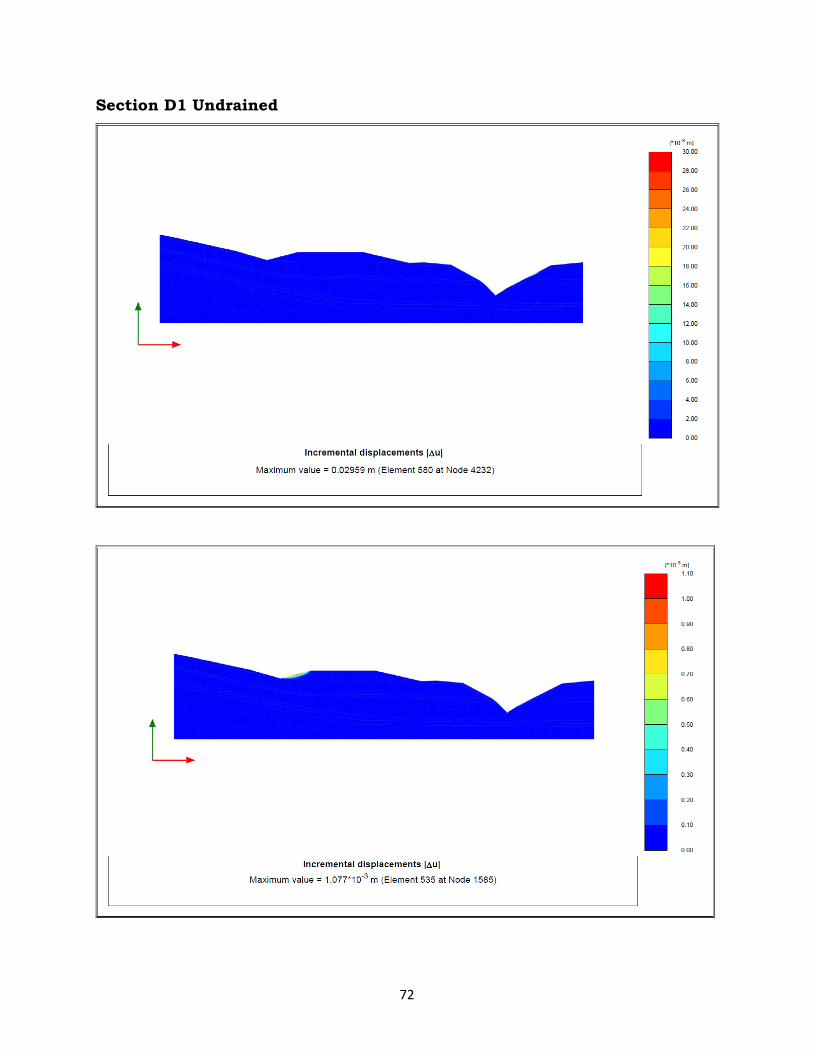
72

Section D1 Undrained

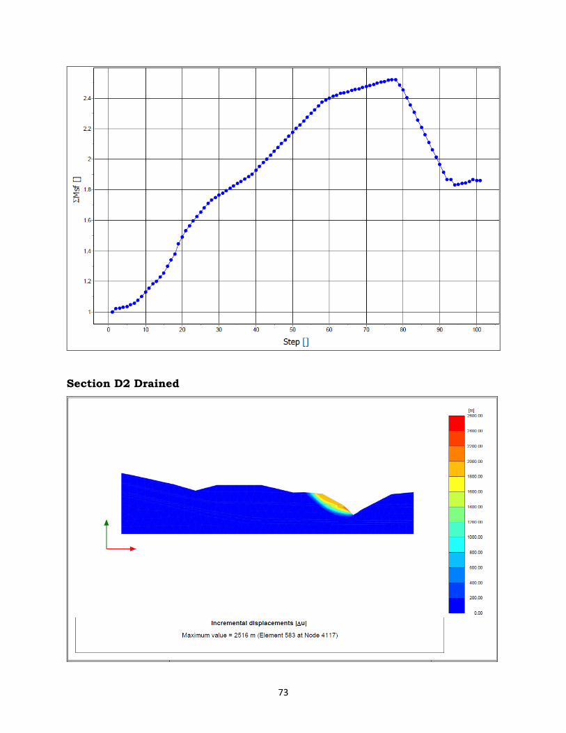
73

Section D2 Drained

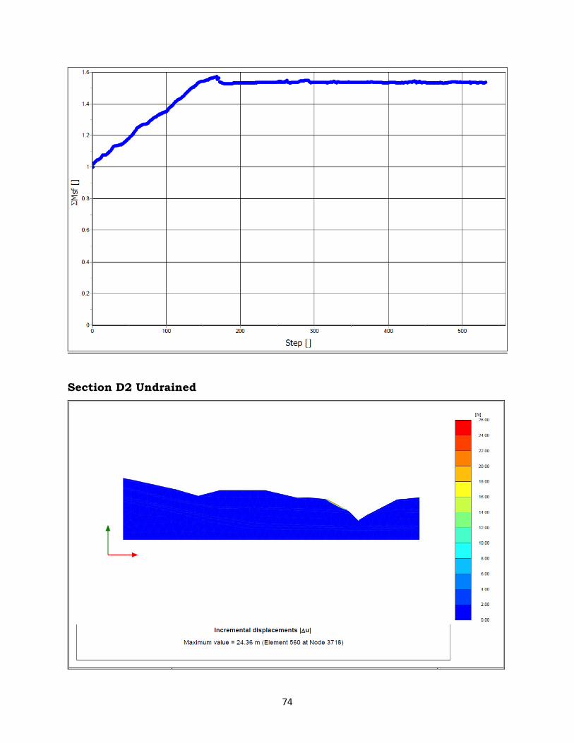
74

Section D2 Undrained

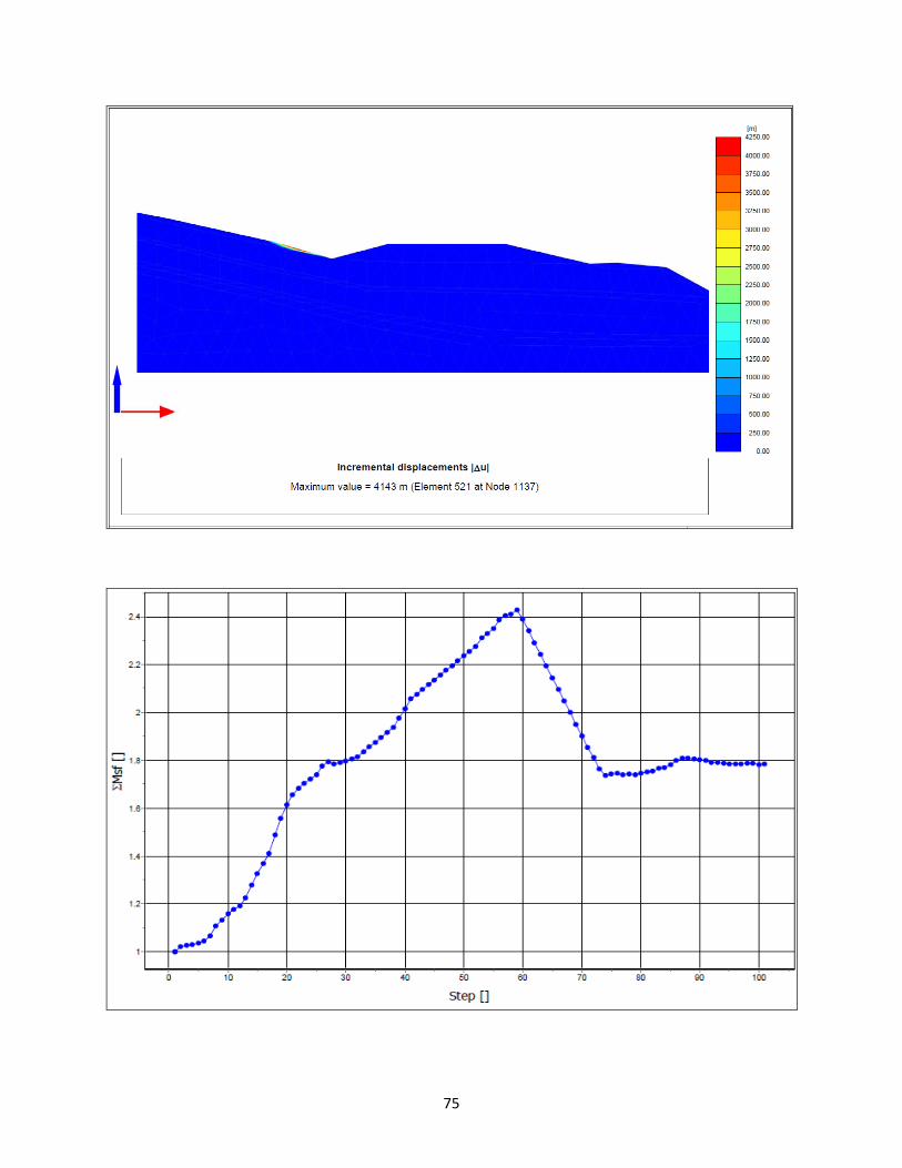
75

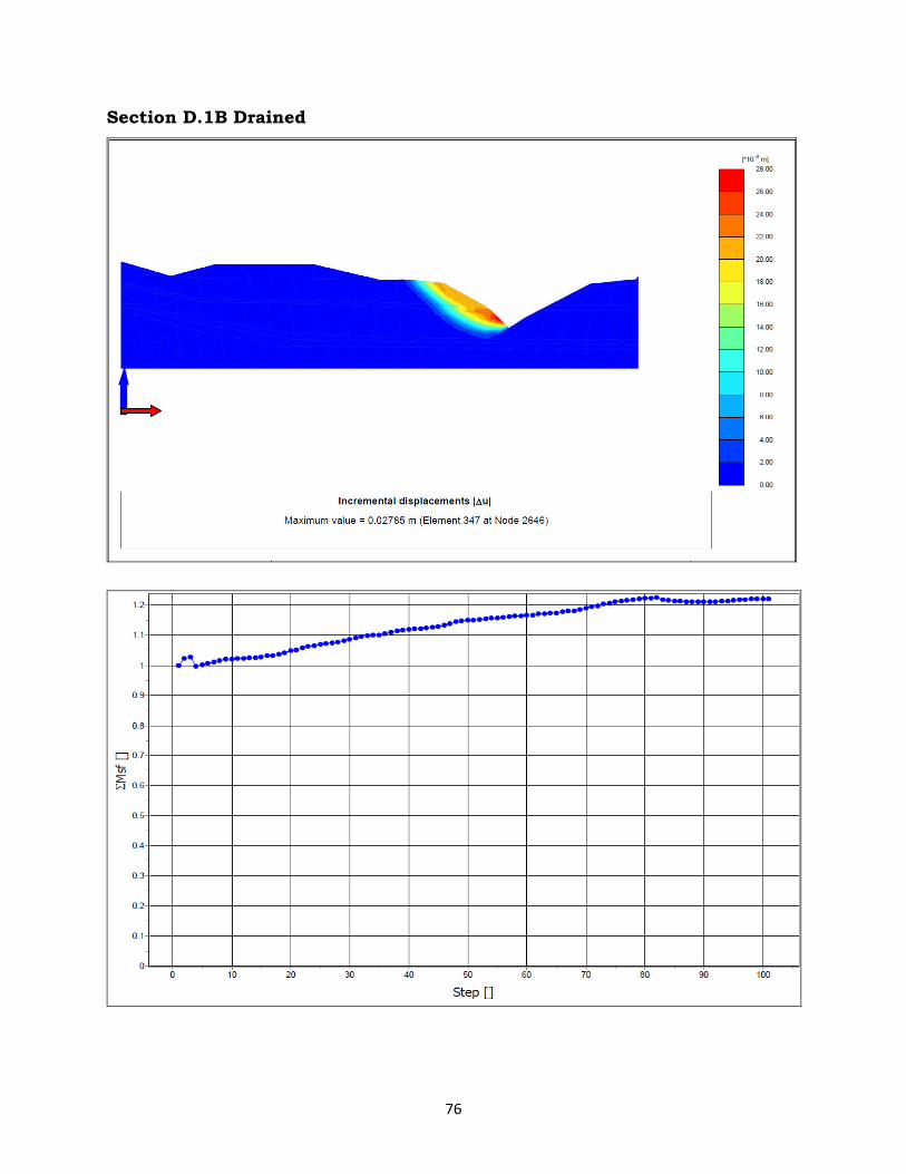
76

Section D.1B Drained

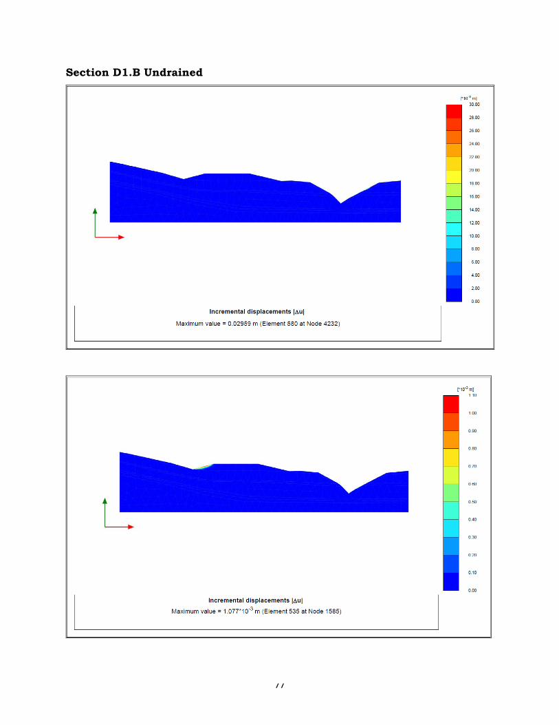
77

Section D1.B Undrained

78

Section D.2B Drained

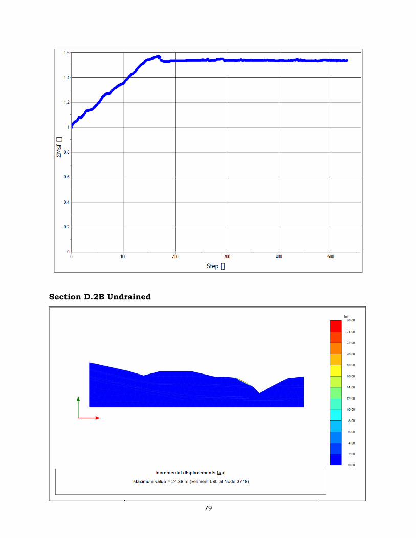
79

Section D.2B Undrained

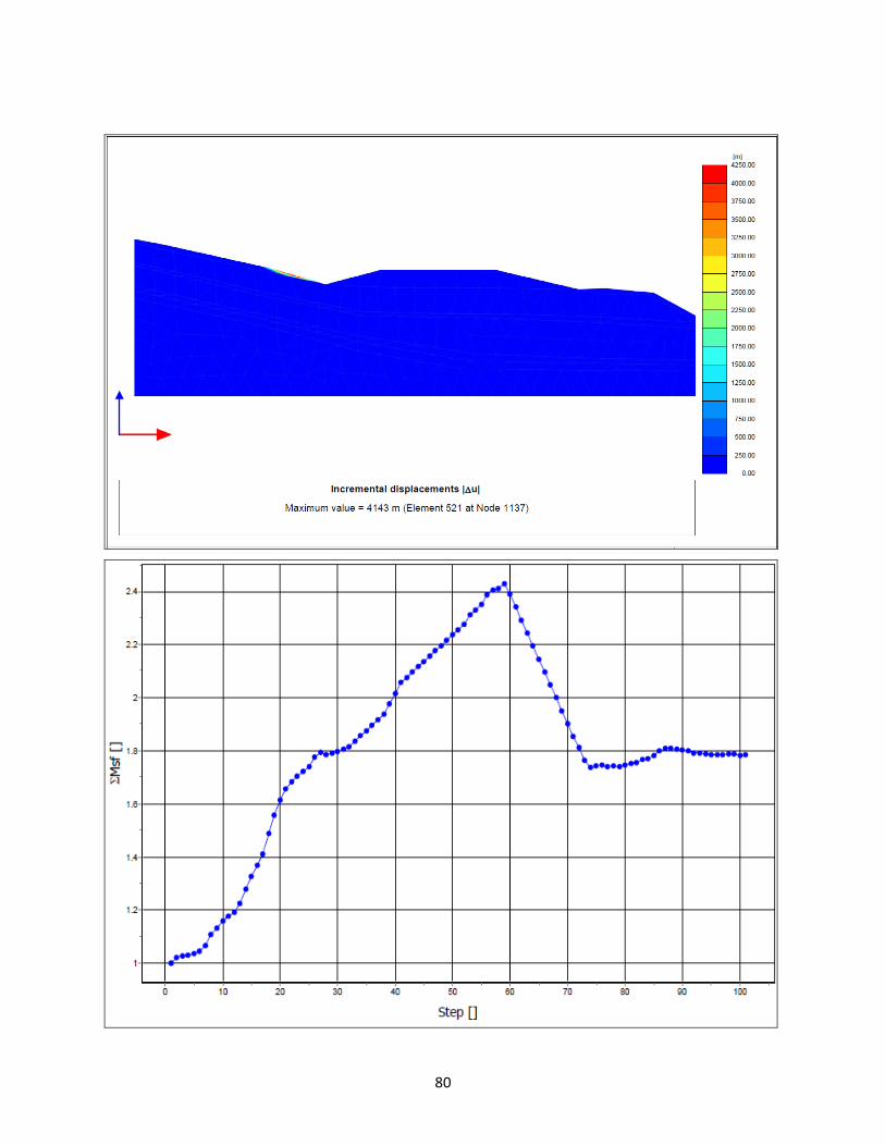
80

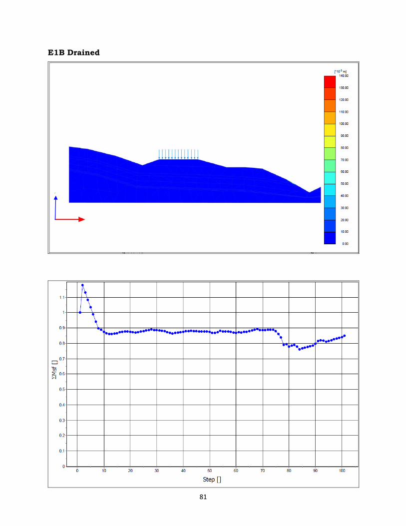
81

E1B Drained

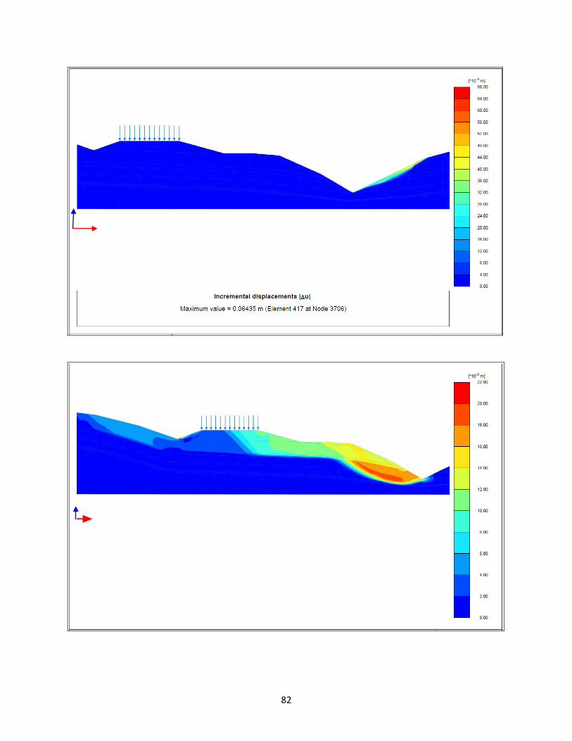
82

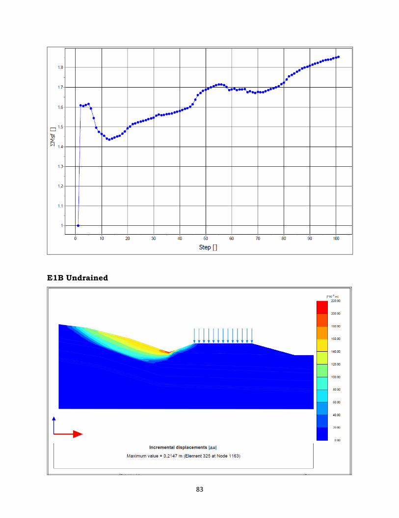
83

E1B Undrained

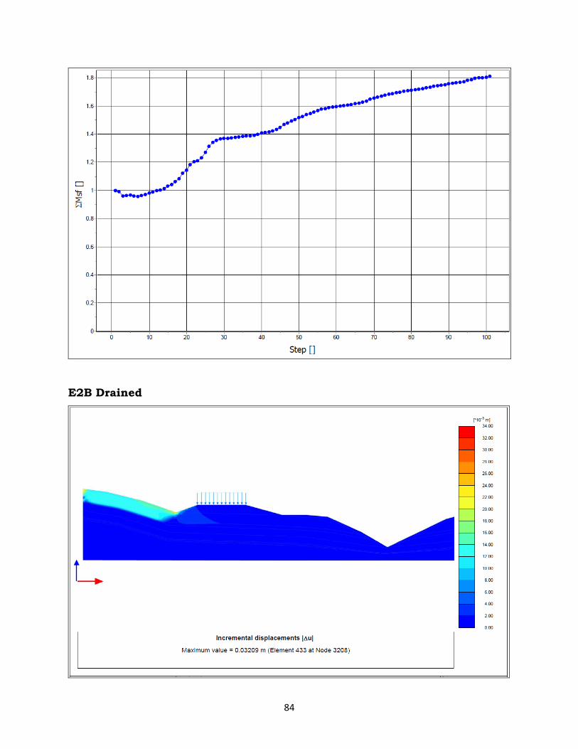
84

E2B Drained

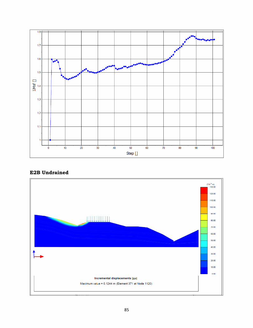
85

E2B Undrained

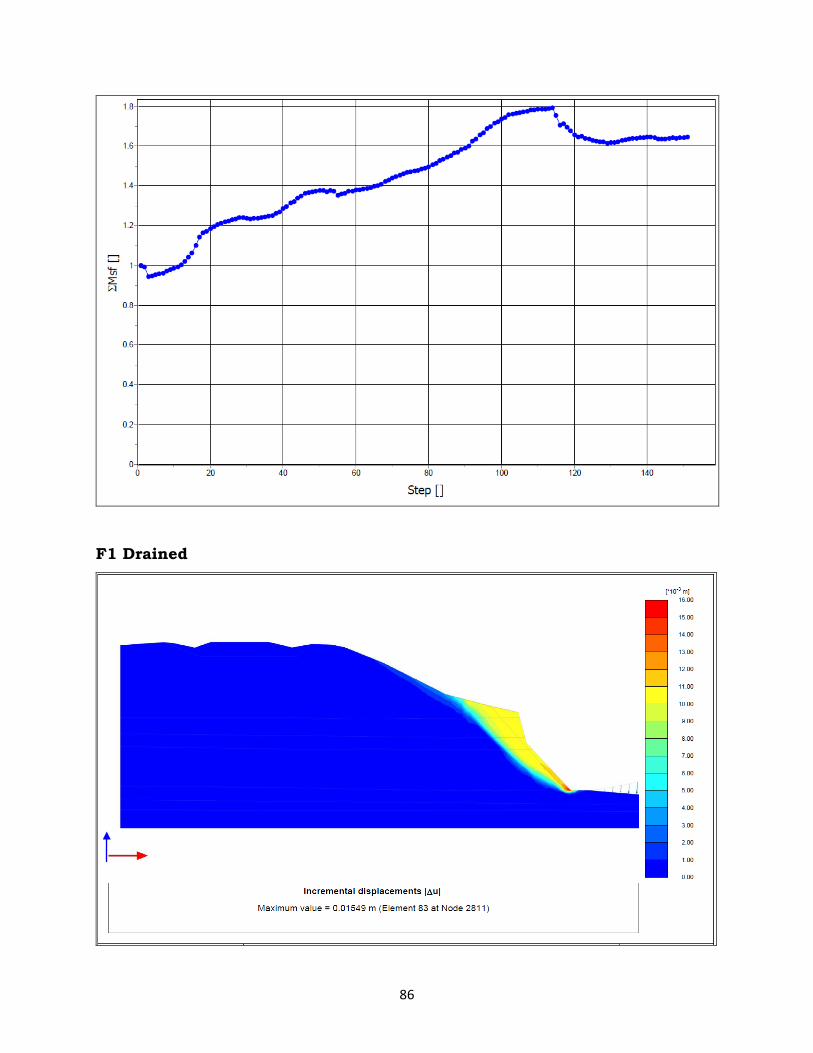
86

F1 Drained

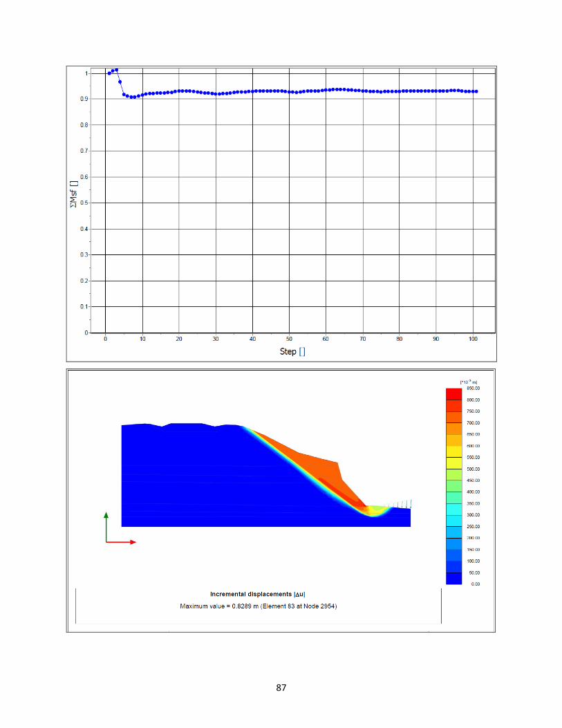
87

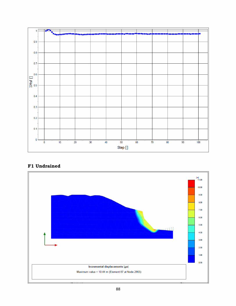
88

F1 Undrained

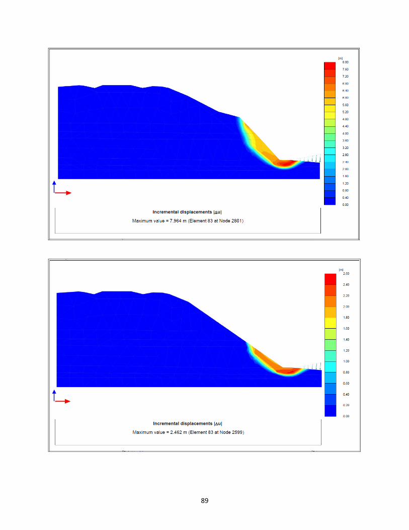
89

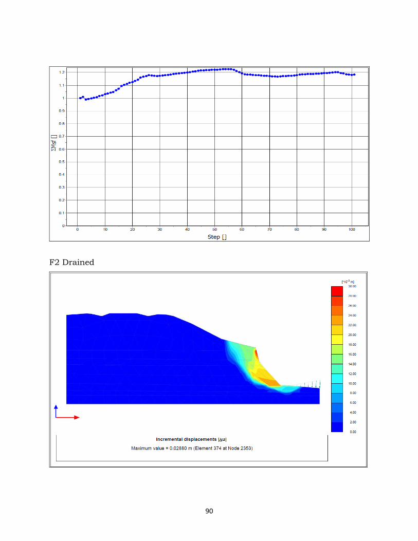
90

F2 Drained

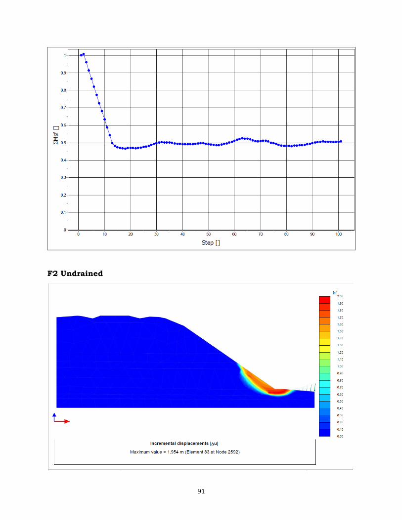
91

F2 Undrained

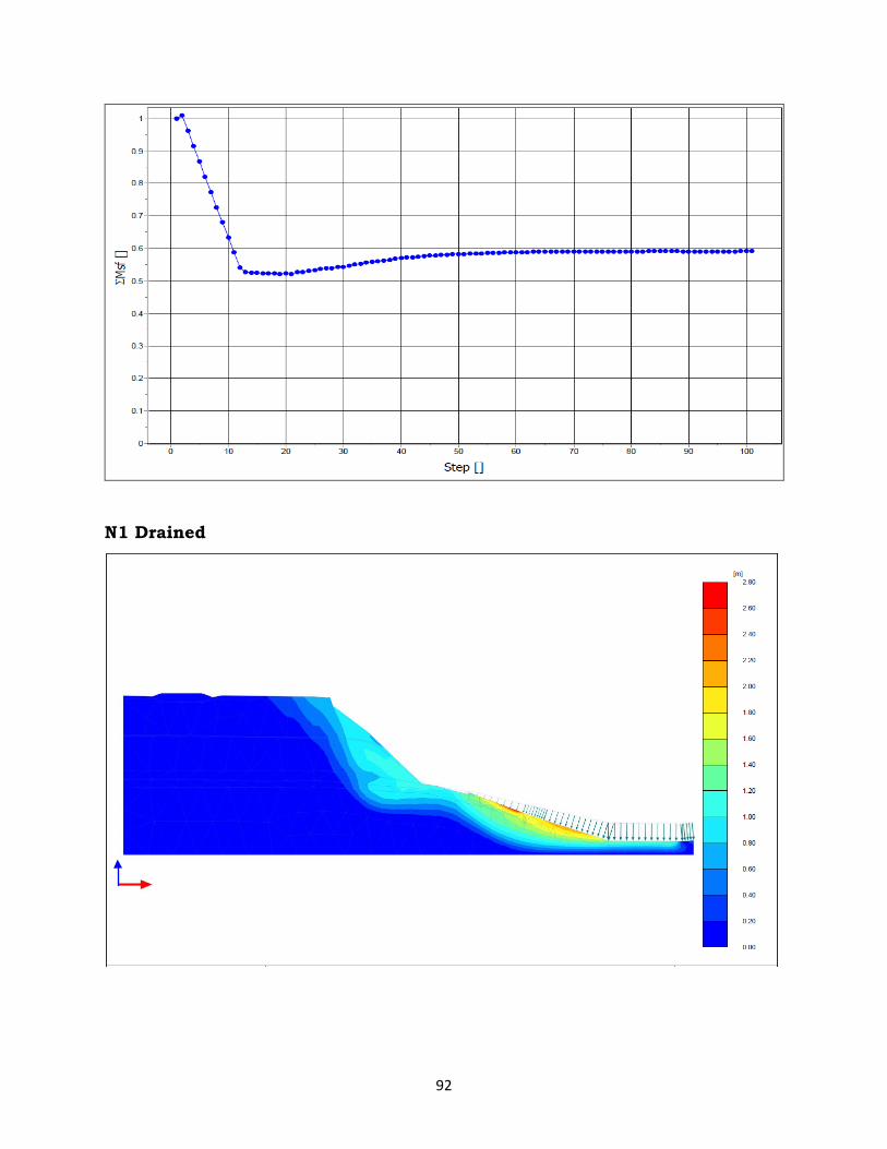
92

N1 Drained

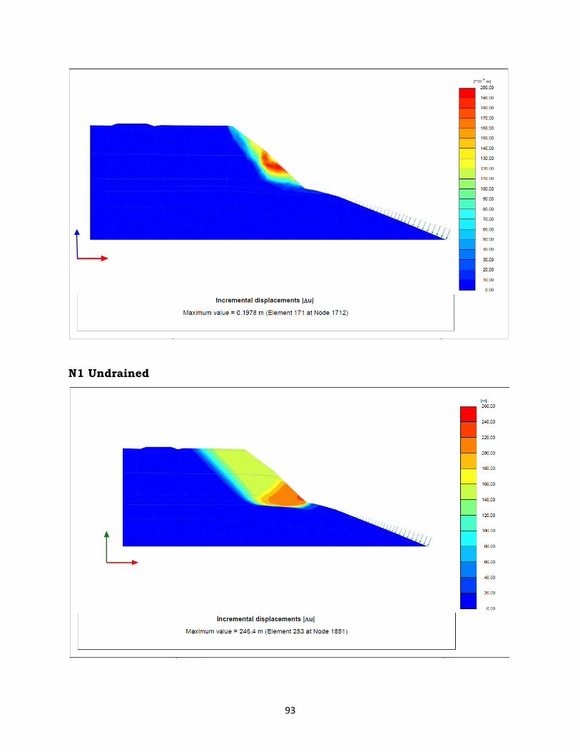
93

N1 Undrained

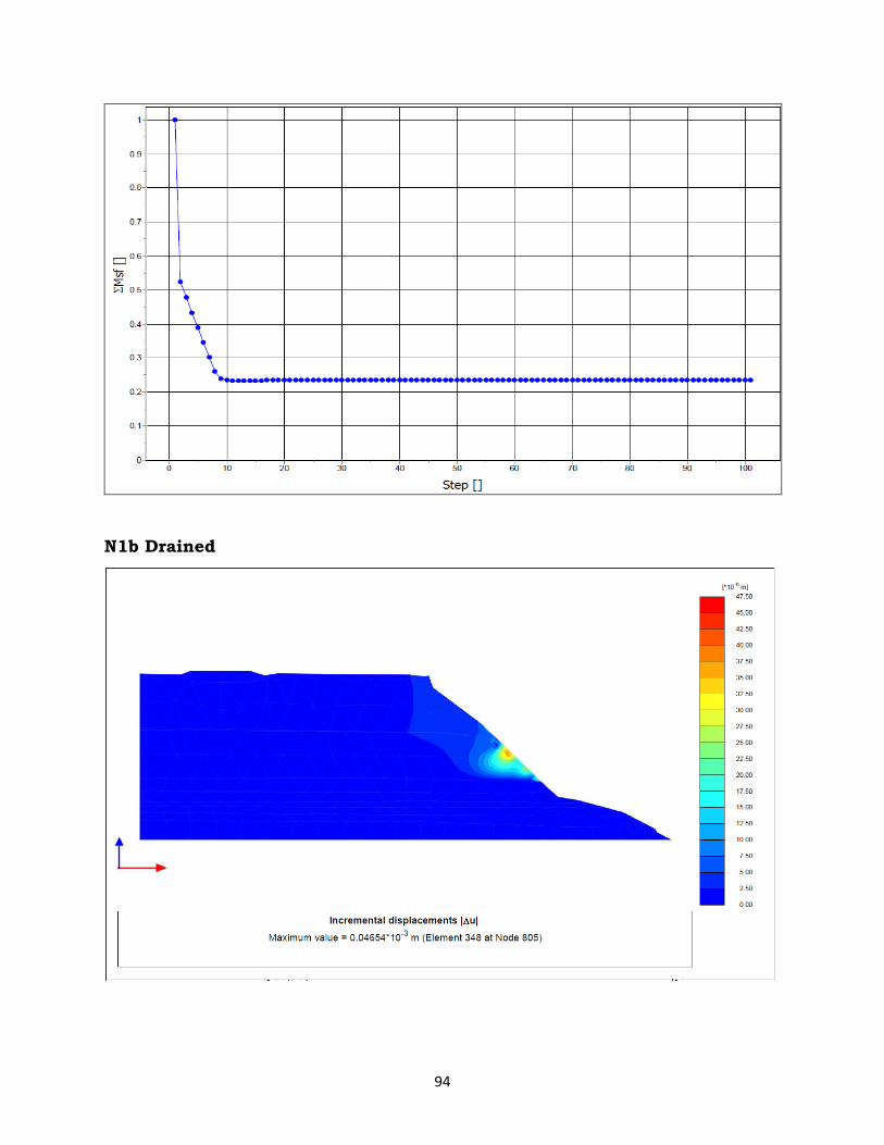
94

N1b Drained

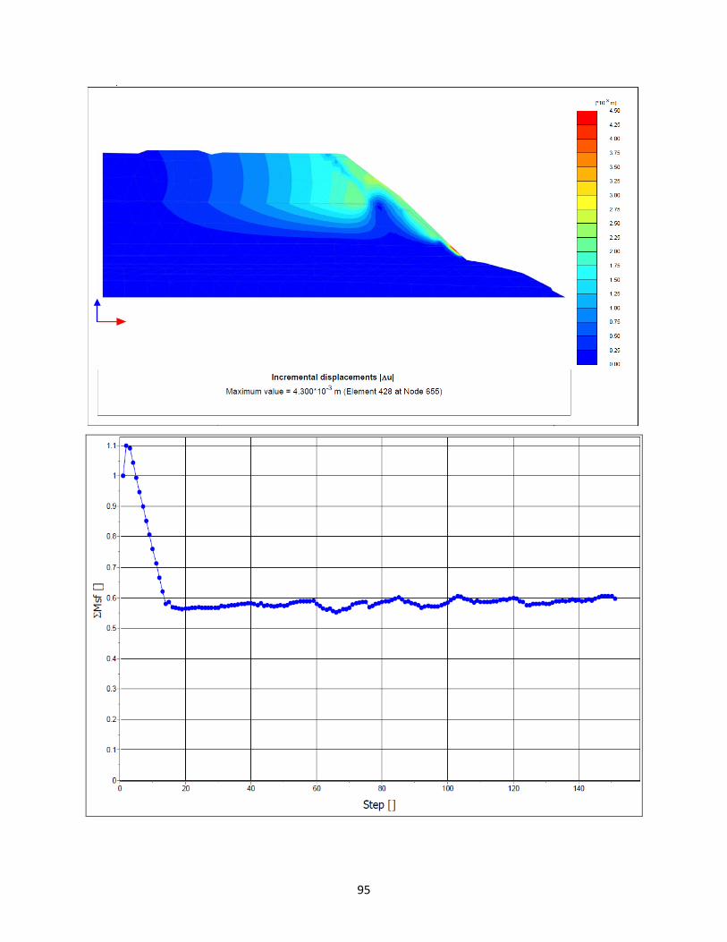
95

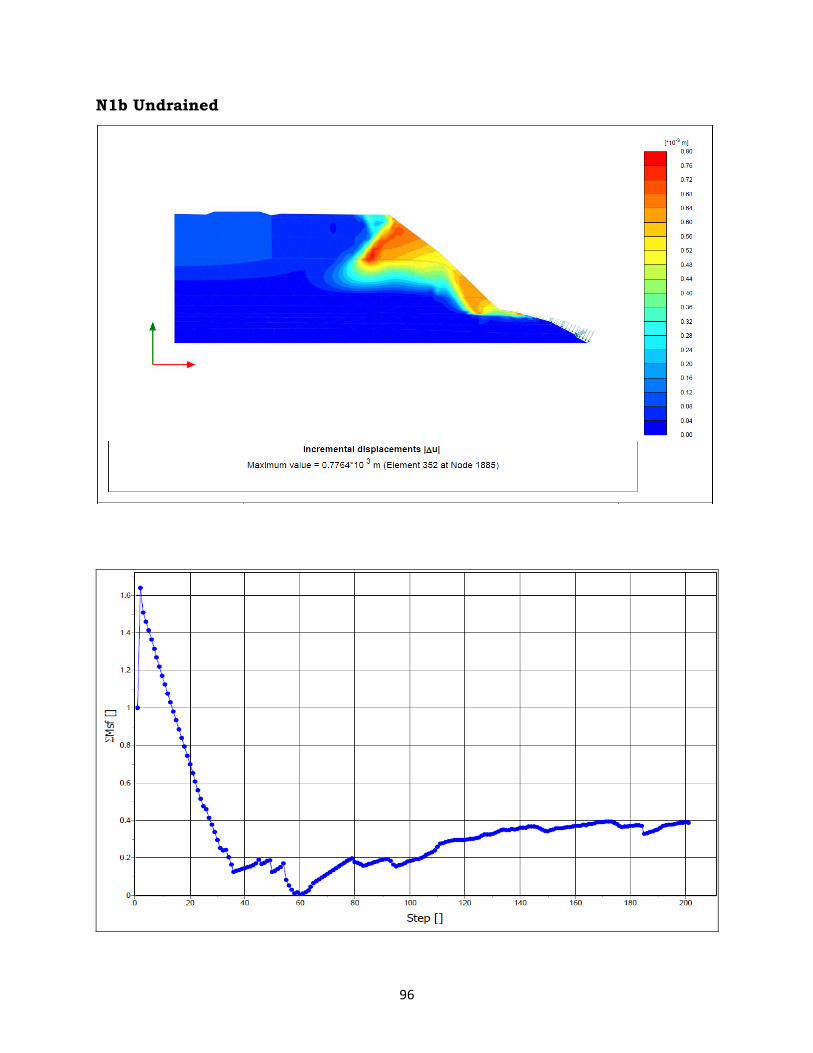
96

N1b Undrained

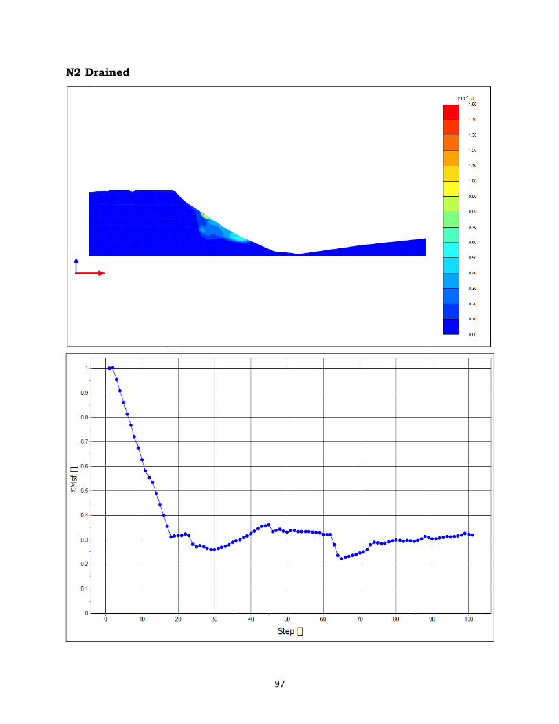
97

N2 Drained

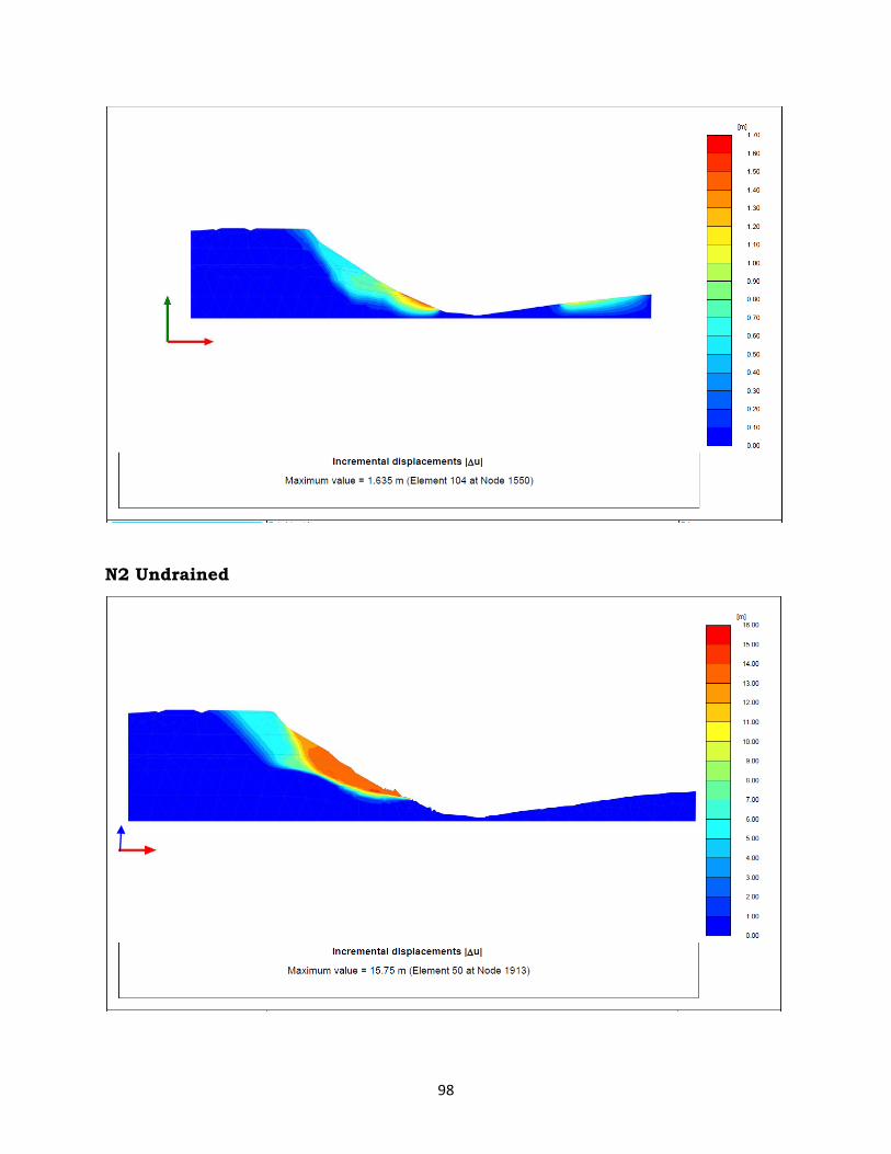
98

N2 Undrained

99

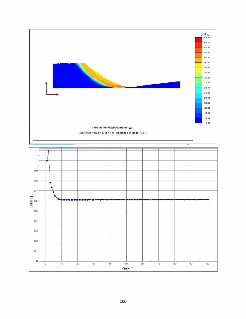
100

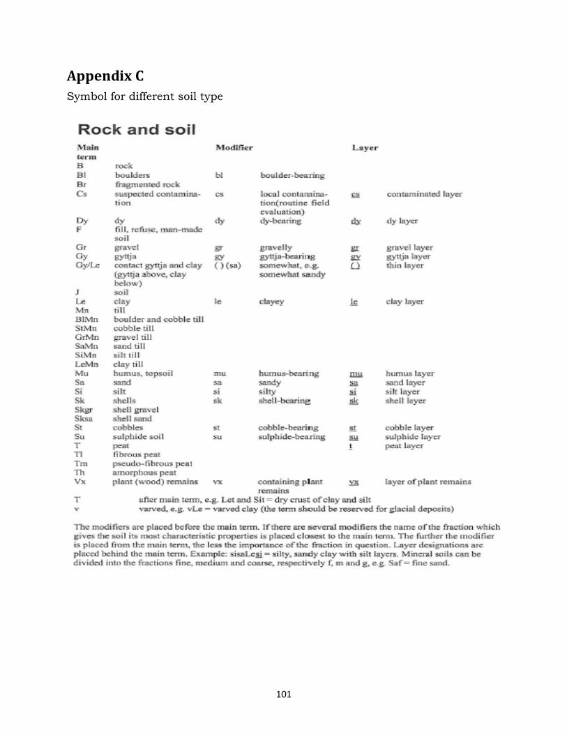
101

Appendix C Symbol for different soil type

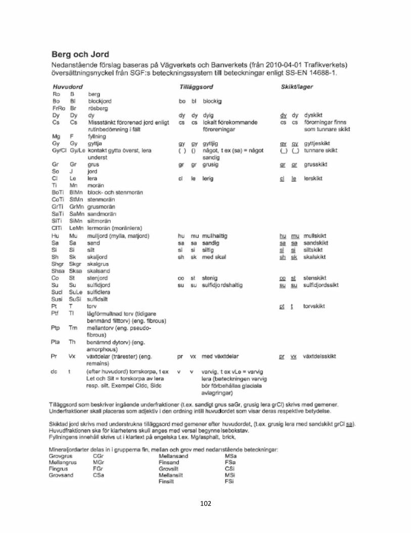
102