Embed Size (px)
Citation preview
MASTER IN
FINANCE
MASTER’S FINAL ASSIGNMENT
DISSERTATION HOW EFFICIENT IS THE PORTUGUESE STOCK MARKET?
SÓNIA MELÂNIA OLIVEIRA VAZ
DECEMBER - 2012
MASTER IN
FINANCE
MASTER’S FINAL ASSIGNMENT
DISSERTATION HOW EFFICIENT IS THE PORTUGUESE STOCK MARKET?
SÓNIA MELÂNIA OLIVEIRA VAZ ORIENTATION:
RAQUEL M. GASPAR CO-ORIENTATION:
ANTÓNIO DA ASCENSÃO COSTA
DECEMBER – 2012
Sónia Vaz How Efficient is the PSI-20? i
i
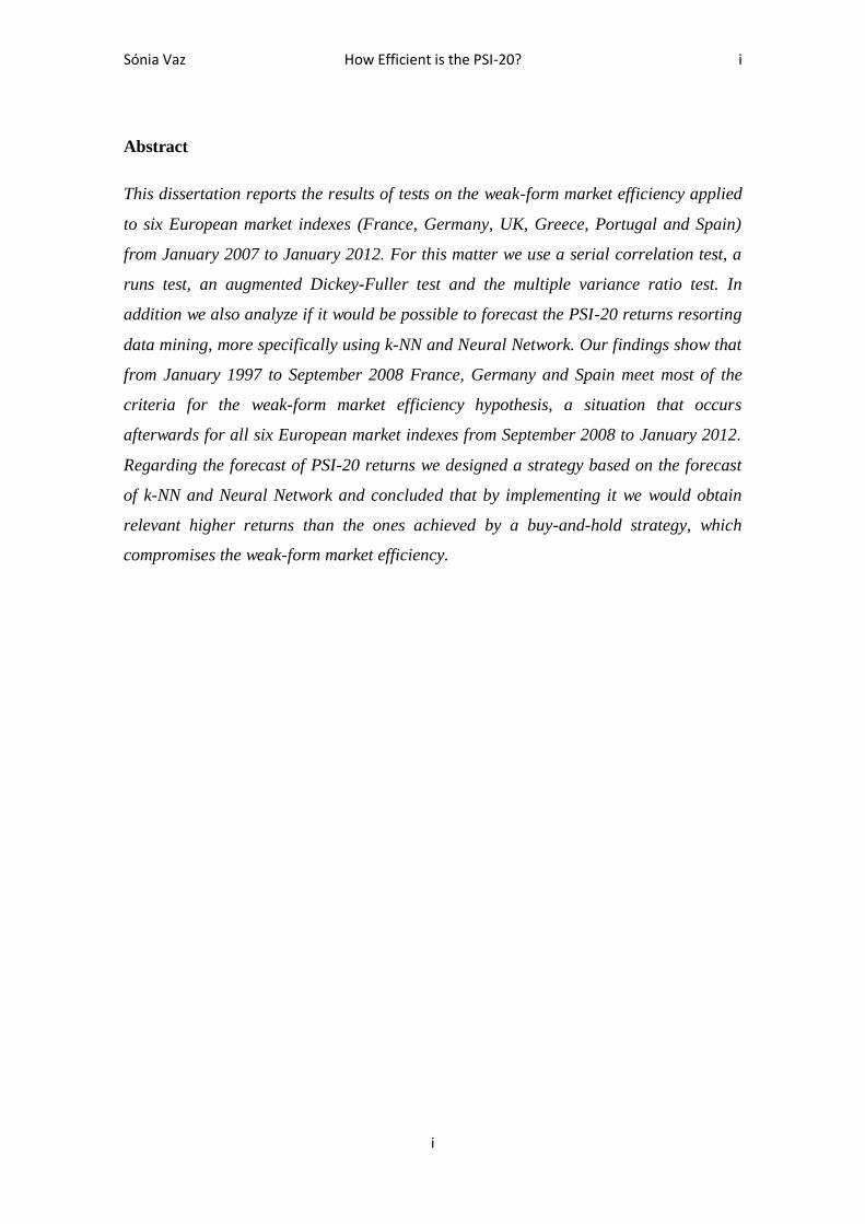
Abstract
This dissertation reports the results of tests on the weak-form market efficiency applied
to six European market indexes (France, Germany, UK, Greece, Portugal and Spain)
from January 2007 to January 2012. For this matter we use a serial correlation test, a
runs test, an augmented Dickey-Fuller test and the multiple variance ratio test. In
addition we also analyze if it would be possible to forecast the PSI-20 returns resorting
data mining, more specifically using k-NN and Neural Network. Our findings show that
from January 1997 to September 2008 France, Germany and Spain meet most of the
criteria for the weak-form market efficiency hypothesis, a situation that occurs
afterwards for all six European market indexes from September 2008 to January 2012.
Regarding the forecast of PSI-20 returns we designed a strategy based on the forecast
of k-NN and Neural Network and concluded that by implementing it we would obtain
relevant higher returns than the ones achieved by a buy-and-hold strategy, which
compromises the weak-form market efficiency.

Sónia Vaz How Efficient is the PSI-20? ii
ii
Acknowledgements
This dissertation would not be possible without the support of my family and friends,
who I would like to thank.
More specifically I would like to thank Jorge Moreira, master student at FEUP, who
explained me how the Rapid Miner works and gave me some much needed help on
understanding the designing of the data mining algorithms.
Also a thank you note for all the support given for my coworkers at PremiValor
Consulting.
Finally it is important to thank the orientation of both Professor Raquel M. Gaspar and
Professor António Costa, which was essential in this process.

Sónia Vaz How Efficient is the PSI-20? iii
iii
Index
Abstract ..................................................................................................................................... i
Acknowledgements ................................................................................................................... ii
1. Introduction .......................................................................................................................... 1
2. Literature Review.................................................................................................................. 2
3. Methodology ......................................................................................................................... 5
3.1 Classical Efficiency tests ................................................................................................. 6
3.1.1 Correlations .............................................................................................................. 6
3.1.2 Runs Test ................................................................................................................. 8
3.1.3 Unit Root Tests ......................................................................................................... 9
3.1.4 Variance Ratio Tests ............................................................................................... 10
3.2 RapidMiner (data mining) approach .............................................................................. 13
3.2.1 W-ZeroR ................................................................................................................ 13
3.2.2 K-NN ..................................................................................................................... 14
3.2.3 Neural Network ...................................................................................................... 14
4. The Data ............................................................................................................................. 15
5. Results ................................................................................................................................ 18
5.1 Classical Efficiency tests ............................................................................................... 18
5.1.1 Correlations ............................................................................................................ 18
5.1.2 Runs Test ............................................................................................................... 21
5.1.3 Unit Root Tests ....................................................................................................... 22
5.1.4 Variance Ratio Tests ............................................................................................... 22
5.1.5 Summary of Tests Results....................................................................................... 25
5.2 RapidMiner (data mining) approach .............................................................................. 26
5.2.1 W-ZeroR ................................................................................................................ 28
5.2.2 K-NN ..................................................................................................................... 29
5.2.3 Neural Network ...................................................................................................... 31
5.2.4 Can we beat the market? ......................................................................................... 33
6. Conclusions ........................................................................................................................ 34
Bibliography ........................................................................................................................... 35
Appendixes ............................................................................................................................. 38
Sónia Vaz How Efficient is the PSI-20? iv
iv
Table Index
Table I. Descriptive statistics................................................................................................... 17
Table II. Autocorrelation, Partial Autocorrelation and Joint correlation (Ljung-Box Q-statistic
probability) ............................................................................................................................. 19
Table III. Are yesterday’s returns statiscally significante for today’s returns? .......................... 20
Table IV. Runs Test ................................................................................................................ 21
Table V. Unit Root Tests......................................................................................................... 22
Table VI. Variance ratio test for lags 2, 5, 10, 30 as well as joint variance ratio test ................. 24
Table VII. Summary of Previous Test Results: Is the random walk hypothesis rejected? .......... 26
Table VIII. Performance of the algorithm W-ZeroR ................................................................ 28
Table IX. Performance of the algorithm k-NN ......................................................................... 29
Table X. Performance of the algorithm Neural Net .................................................................. 31
Table XI. Results of implementing the algorithms strategy ...................................................... 33
Sónia Vaz How Efficient is the PSI-20? v
v
Index of Figures
Figure 1: The k-nearest neighbor classification algorithm ........................................................ 14
Figure 2. A multilayer feed-forward neural network ................................................................ 15
Figure 3. Stock Market Indexes - Closing Prices - 1997 to 2012 .............................................. 16
Figure 4. Example of a RapidMiner process ............................................................................ 27
Figure 5. PSI-20 forecasting results with W-ZeroR: data from 01/01/97 to 12/09/08 ................ 29
Figure 6. PSI-20 forecasting results with W-ZeroR: data from 15/09/08 to 31/01/12 ................ 29
Figure 7. PSI-20 forecasting results with k-NN: data from 01/01/97 to 12/09/08 ...................... 31
Figure 8. PSI-20 forecasting results with k-NN: data from 15/09/08 to 31/01/12 ...................... 31
Figure 9. PSI-20 forecasting results with Neural Network: data from 01/01/97 to 12/09/08 ...... 32
Figure 10. PSI-20 forecasting results with Neural Network: data from 15/09/08 to 31/01/12 .... 32

Sónia Vaz How Efficient is the PSI-20? 1
1
1. Introduction
The theory of market efficiency has been widely discussed in the financial literature
over the years. However no undisputable conclusion has been reached. Being so, in this
dissertation we choose to analyze the weak form market efficiency in six European
indexes (France, Germany, UK, Greece, Spain and Portugal) from January 1997 to
January 2012.
First, to fully understand this matter, we will do a literature review.
Then we will explain the methodology pursued which will be divided in two
approaches. The first one is the classical efficiency tests, which concerns the
correlations, runs test, unit root test and variance ratio test. The second one relies on the
data mining approach using algorithms as W-ZeroR, k-NN and Neural Networks.
The chapter that follows concerns the performance of the six European indexes priory
mentioned on the classical efficiency tests as well as an effort of forecasting the PSI-20
returns using the algorithms previously stated. In addition we will also develop a
strategy that attempts to beat the market given the forecasts obtained by the algorithms.
Finally we will discuss all the results on a conclusion chapter.

Sónia Vaz How Efficient is the PSI-20? 2
2
2. Literature Review
According to LeRoy (1989) “at its most general level, the theory of efficient capital
markets it just the theory of competitive equilibrium applied to asset markets” and its
origin dated from the 1930s. In fact, Williams (1938) and Graham & Dodd (1934)
stated that the fundamental value of any security is equal to the discounted cash flow of
that security, which means the actual price should fluctuated around fundamental
values. Being so, analysts began to recommend buying (selling) orders if securities were
priced below (above) fundamental value.
After that, many other authors address the market efficiency hypothesis, as a random
walk model, but it was with Samuelson (1965) that for the first time someone developed
the link between capital market efficiency and martingales, which are in fact, as stated
by LeRoy (1989), “a weaker restriction on asset prices that still captures the flavor of
the random walk arguments”.
Also according to LeRoy (1989) “the dividing line between the ‘prehistory’ of efficient
capital markets, associated with the random walk model, and the modern literature is
Fama’s (1970) survey.” In here, Fama (1970) stated that “in an efficient market prices
"fully reflect" available information” and present three categories to consider: weak
form tests (which the concern is if past returns can predict or explain the future ones),
semi-strong form tests (concerning how quickly prices adjust to the public information
available, e.g. announcements of annual earnings, etc.) and strong form tests (to
evaluate if an investor, or group of investors, have private information that is not
entirely reflected in market prices). Later on, Fama (1991) proposes that weak form
tests also covers “the more general area of tests for return predictability, which also
includes the burgeoning work on forecasting returns with variables like dividend yields
and interest rates”. In this article, he also proposes changing the title from semi-strong
form test to event studies and from strong tests to tests for private information.
Therefore, the question we have to pose is if the analysis of past returns can provide us
information about future returns. According to Jensen & Benington (1970) “the random
walk and martingale efficient market theories of security price behavior imply that stock
market trading rules based solely on the past price series cannot earn profits greater than
those generated by a simple buy-and-hold policy”. However some analysts (technical

Sónia Vaz How Efficient is the PSI-20? 3
3
analysts) believe that the past gives them clues about the future and operate in the basis
of the psychology of the market.
Allen & Taylor (2002) affirm that “technical, or chartist, analysis of financial markets
involves providing forecasts or trading advice on the basis of largely visual inspection
of past prices, without regard to any underlying economic or ‘fundamental’ analysis”
and Artus (1995) defends that there are two groups of investors: the fundamental ones
and the technical ones. This author admits that technical investors will buy stocks due to
an upward market movement (bull markets) and sell it if the market suffers from a
descending movement (bear markets). Being so, if they are in a significant number, they
will be able to influence the stock price, and consequently the market will operate
according to their expectations.
As we shown, many were the authors that over the years refuted technical analysis as a
way of achieving better results than with a buy and hold strategy. Even so in the sixty’s
Levy (1967, 1968) already claim to have achieved a trading rule that, on average, earn
significantly more than the buy and hold strategy, which refutes the market efficiency
hypothesis.
Nevertheless, as stated in Ferson et al (2005), “the empirical evidence for predictability
in common stock returns remains ambiguous, even after many years of research”. These
authors analyze the Standard & Poor’s stock index from 1885 to 2001 in order to make
an indirect inference regarding the time-variation in expected stock returns, through the
comparison of the unconditional sample variances with the estimates of expected
conditional variances. Ferson et al (2005) then conclude concerning weak-form tests
that “while the older historical data suggests economically significant predictability in
the market index, there is little evidence of weak-form predictability in modern data”
and “find small but economically significant predictability” concerning semi-strong
form tests.
Smith & Ryoo (2003) tested the hypothesis of the stock market prices indexes follow a
random walk for five markets (Greece, Hungary, Poland, Portugal and Turkey) using
the multiple variance ratio test. In fact, according to Smith & Ryoo (2003) “in markets
that are weak-form efficient, equity prices completely reflect all of the information
contained in the past history of prices and do not convey information about future
Sónia Vaz How Efficient is the PSI-20? 4
4
changes in prices. If they did convey such information there would be profit-making
opportunities for investors and so markets would be imperfect”. For this matter they
used weekly data, beginning in the third week of April 1991 and ending in the last week
of August 1998 and were able to conclude that only the Turkey market was efficient.
Worthington & Higgs (2004) also study the random walk and weak-form market
efficiency in European markets, covering twenty European markets: sixteen developed
markets (Austria, Belgium, Denmark, Finland, France, Germany, Greece, Ireland, Italy,
Netherlands, Norway, Portugal, Spain, Sweden, Switzerland and the United Kingdom)
and four emerging markets (Czech Republic, Hungary, Poland and Russia). It is
important to test this hypothesis because, as stated in Worthington & Higgs (2004) “the
presence (or absence) of a random walk has implications for investors and trading
strategies, fund managers and asset pricing models, capital markets and weak-form
market efficiency, and consequently financial and economic development as a whole”.
To analyze if the markets chosen follow a random walk they made several tests as serial
correlation coefficient, runs tests, Augmented Dickey-Fuller (ADF), Phillips-Perron
(PP), Kwiatkowski, Phillips, Schmidt and Shin (KPSS) unit root tests and multiple
variance ratio (MVR). The conclusion was that only Germany, Ireland, Portugal,
Sweden and the United Kingdom, regarding the developed markets, and Hungary,
regarding the emerging markets, follow a random walk.
In addition Borges (2010) too assessed the random walk hypothesis for European
countries (UK, France, Germany, Spain, Greece and Portugal) from January 1993 to
December 2007, for both daily and weekly data, and by using runs test and variance
ratio test concluded that the hypothesis of market efficiency is not rejected for Germany
and Spain.
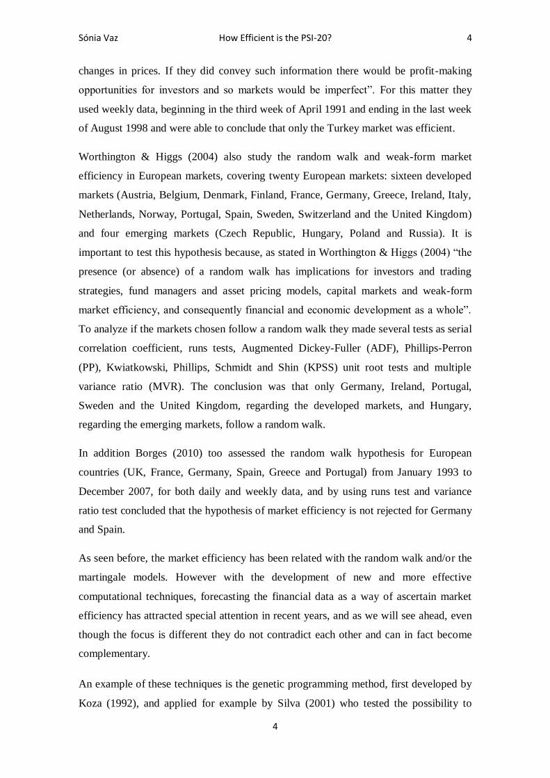
As seen before, the market efficiency has been related with the random walk and/or the
martingale models. However with the development of new and more effective
computational techniques, forecasting the financial data as a way of ascertain market
efficiency has attracted special attention in recent years, and as we will see ahead, even
though the focus is different they do not contradict each other and can in fact become
complementary.
An example of these techniques is the genetic programming method, first developed by
Koza (1992), and applied for example by Silva (2001) who tested the possibility to
Sónia Vaz How Efficient is the PSI-20? 5
5
obtain an exceptional profitability, forecasting BVL Geral stock index evolution. The
results show that this type of procedure can be used with some effectiveness in
predicting the evolution of the index value, which can reveal the nonexistence of weak
efficiency in the Portuguese stock market.
Another technique widely used is the data mining concept which employs algorithms as
nearest neighbor1 and neural networks. If “nearest neighbor forecasting models are
attractive with their simplicity and the ability to predict complex nonlinear behavior”
(Isfan et al, 2010), the neural networks, despite more complex, “represent one of the
most powerful tools for non-parametric regression analysis” (Cabarkapa et al, 2010).
Hill et al (1996) evaluate traditional statistical models (as exponential smoothing, for
example) and neural networks for time series forecasting and concluded that, regarding
the quarterly and monthly data, the neural network model did significantly better
forecasting than the traditional statistical.
Also McNelis (2005) examined how well neural network methods perform, using for
that several examples as forecasting the automotive industry, the corporate bonds, the
inflation, the credit card default and bank failure, and others.
Recently, Isfan et al (2010), forecast the Portuguese stock market using the Hurst
exponent as well as nearest neighbor algorithm and artificial neural networks (ANN2)
and they conclude that although neural networks were not “perfect in their prediction,
they outperform all other methods”.
3. Methodology
In this study we analyze the weak form market efficiency using two distinct approaches.
The first approach is the classical one as proposed by Worthington & Higgs (2004) and
later used by Borges (2008, 2011), for the hypothesis of stock market indexes’ returns
following a random walk (or a martingale process, which is in practice less restrictive).
Admitting that, the following tests will be done: correlations tests (with analysis of the
1 This can also be written as k-NN. 2 ANNs were often just called neural networks and, since the RapidMiner 5.0 uses this terminology, from
now on we will refer them just as neural networks.

Sónia Vaz How Efficient is the PSI-20? 6
6
autocorrelation, partial autocorrelation, joint correlation and a linear regression that
allow us to conclude if yesterday’s returns are statistically significant for today’s
returns), a runs test, the augmented Dickey-Fuller test to analyze the existence of an unit
root and finally the multiple variance ratio test using different approaches. It is worth
mentioning that the softwares Eviews and SPSS were a useful tool for those tests.
The second approach relies on the software RapidMiner 5.0 to analyze if it is possible to
predict the PSI-20 returns using several algorithms: W-ZeroR, k-NN and Neural
Network.
3.1 Classical Efficiency tests
3.1.1 Correlations
We can define correlation as the degree of linear association between two variables as
mentioned in Brooks (2002) and it is important to analyze the correlation of the returns
because as stated by Borges (2008) “if the stock market indexes returns exhibit a
random walk, the returns are uncorrelated at all leads and lags”.
In this point we will analyze the folowing: the individual autocorrelation, the individual
partial autocorrelation, joint correlation using the Ljung Box Q-statistic and finally the
correlation on lag 1 with more detail.
The difference between the autocorrelation and partial autocorrelation lies in while the
first is related to the moving average process, the second relates to the autoregressive
process.
A moving average model is a linear combination of terms in a white noise process3 and
using the notation presented in Brooks (2002), a moving average process of order q,
MA(q), can be expressed as:
(1) 1 1 2 2 ...t t t t q t qy u u u u
Being ut (t = 1, 2, …) the white noise process with E(ut) = 0 and var(ut) = σ2
3 Brooks (2002) states that «a white noise process is one with no discernible structure». So, the definition
of a white noise process is E(yt) = µ var(yt) = σ2 and
where stands for the
autocorrelation coefficient at lag t-r.
Sónia Vaz How Efficient is the PSI-20? 7
7
^
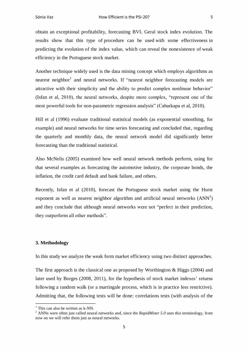
On the other hand, an autoregressive model is one in which the current value of a
variable, y, depends only on the values that the variable had in previous periods,
plus an error term. Using the notation expressed in Brooks (2002), an autoregressive
model of order p, AR(p) can be written as:
(2) 1 1 2 2 ...t t t p t p ty y y y u
Where ut is a white noise disturbance term.
Now that we clarify those concepts it is important to define the individual tests:
a) Regarding the autocorrelation the hypothesis will be
H1: if otherwise
And then we will reject H0 at 5% if
Where T is the number of observations
b) Regarding the partial correlation the hypothesis will be
H1: if otherwise
And then we will reject H0 at 5% if
In order to test for joint null correlations coeficienst, the hypothesis are the following:
H0: The data are independently distributed
H1: The data are not independently distributed
In this matter we aplly the Ljung Box Q-statistic joint test, expressed in Brooks (2002)
as:
(3) 2
2
( )
1
( ) ( 2 χ)m
km
k
Q m T TT k
Sónia Vaz How Efficient is the PSI-20? 8
8
Where T is the sample size, m the maximum lag considered (in this thesis, m equals
100) and is the sample autocorrelation coeficient.
Therefore we will reject the null hypotesis if Q-stat or if prob 0,05.
At last our purpose is to analyze the lag 1 with more detail. In fact, as stated by Peña
(2005), the confidence levels that we use to analyze if the autocorrelations are equal to
zero, are asymptotic and not acurate enough for the firsts lags, being necessary further
examination. Therefore, in order to do it, we raise the question “are the yesterday’s
returns statiscally significant to today’s returns?” which can be done through a linear
regression:
(4) 0 1(log( )) (log( ( 1)) ti i
where i referes to market index4 and AR(1) an autoregressive of order 1.
3.1.2 Runs Test
The runs test is a non-parametric statistical test that determines if the elements of the
sequence are mutually independent, as should happen under the weak-form efficient
market hypothesis.
Following the methodology proposed in Borges (2010, 2011), we will classify a
positive return (+) if the return is above media and a negative return (-) if the return is
below media. Then, according to Borges (2010), “the runs test is based on the premise
that if price changes (returns) are random, the actual number of runs (R) should be close
to the expected number of runs ( )” under the null hypothesis of the elements of the
series are mutually independent. Also note that n+ refers to the number of positive
returns and n- to the number of negative returns, which imply n=n++n-. Assuming large
numbers of observations the following test will be made:
(5) (0,1)R
R
RZ N
4 For example
Sónia Vaz How Efficient is the PSI-20? 9
9
where 2
1R
n n
n and
2
2 (2 )
( 1)R
n n n n n
n n
3.1.3 Unit Root Tests
The unit root tests are used to determine whether a variable time series is non stationary,
using for that purpose an autoregressive model. The first work on this matter was
developed by Dickey and Fuller (Fuller, 1976; Dickey and Fuller, 1979), being the null
hypothesis the series having a unit root versus the series being stationary.
According to Brooks (2002) the regression used for the Dickey-Fuller test is:
(6) 1t t ty y u
Where yt represents the prices at time t, and ut a white noise.
This will examine the null hypothesis of ψ = 0 against ψ < 0, being the test statistic
defined as:
(7) test stastisticˆ( )SE
However what we will take into account is the augmented Dickey-Fuller (ADF), which
is an augmented version of Dickey-Fuller test and applies the following regression,
using the notation presented in Brooks (2002):
(8) 1
1
p
t t i t i t
i
y t y y u
Where µ is a constant, λt is the coefficient for the trend and αi are coefficients to be
estimated. Note that imposing µ=0 and λt=0 corresponds to modeling a random walk,
using only the constraint λt=0 corresponds to test for a random walk with drift and using
no constraints means testing for a random walk with drift and a deterministic time trend.
It is worth to mentioning that the null hypothesis of ψ = 0 against ψ < 0 remains and
failing to reject the null hypothesis implies that we do not reject that the time series has
the properties of a random walk.
Sónia Vaz How Efficient is the PSI-20? 10
10
3.1.4 Variance Ratio Tests
The variance ratio (VR) test allows to verify whether differences in a series are
uncorrelated, by comparing variances of differences of the returns calculated over
different lags.
The most common approach is the one developed by Lo and MacKinlay (1988, 1989)
which tested the random walk hypothesis under two different null hypothesis: the first
reliyng on homoskedastic increments and the second on heteroskedastic increments.
Assuming yt as the stock price at time t, where t = 1, …, T:
(9) t ty
Where is an arbitrary drift parameter and the random disturbance term. Then, for
the first hypothesis – the homoskedastic random walk hypothesis – Lo and MacKinlay
(1988) assume that are i.i.d.5 Gaussian with variance σ
2 and for the second hypothesis
– the heteroskedastic random walk hypothesis – they assume a less restrictive theory
that “offers a set of sufficient (but not necessary), conditions for to be a martingale
difference sequence (m.d.s.)” (Quantitative Micro Software, LLC, 2009)
Using the notation presented in Quantative Micro Software, LLC (2009), we can define
the mean of first difference and the scaled variance of the q-th difference respectively
as:
(10) 1
1
1ˆ ( )
T
t t
t
y yT
(11) 2 2
1
1ˆ ˆ( ) ( )
T
t t q
t
q y y qTq
With the correspondent Variance Ratio being
(12) 2
2
ˆ ( )( )
ˆ (1)
qVR q
5 i.i.d. stands for independently and identically distributed.
Sónia Vaz How Efficient is the PSI-20? 11
11
where is 1/q the variance of the qth difference and is the variance of the
first difference. Note that under the random walk hypothesis, we must have VR(q) = 1
for all q.
Then, the authors demonstrate that, under the i.i.d. assumption, the variance ratio z-
statistic
(13) 1/2
2
1ˆ( ) ( ) 1 ( )z q VR q s q
is asymptotically N(0,1) where 2 2(2 1)( 1)ˆ ( )
3
q qs q
qT
.
For the m.d.s. assumption, the authors propose a variance ratio z-statistic, which is
robust under heteroskedasticity and follows the standard normal distribution
asymptotically:
(14) 1/2
2
2ˆ( ) ( ) 1 ( )z q VR q s q
Where
21
2
1
2( ) ˆˆ ( )q
j
j
q js q
q
and
2 2
1
2
2
1
ˆ ˆ( ) ( )
ˆ
ˆ( )
T
t j t
t j
jT
t j
t j
y y
y
The procedure above is, as stated by Borges (2010), “devised to test individual VR tests
for a specific q-difference”, however as we mentioned before, under the random walk
hypothesis, we must have VR(q) equal to one for all q. Being so, we will analyze the
joint variance ratio tests proposed by Chow and Denning (1993), which defined
heteroskedastic test statistic as:
(15) 21max ( )i
i mCD T z q
Sónia Vaz How Efficient is the PSI-20? 12
12
This test statistic follows the SMM6 distribution with parameter m and T degrees of
freedom, that is, SMM (α, m, T).
Kim (2006) also developed a VR test, but employing wild bootstrap. We will also
explore Kim’s methodology which consists in computing both individual and joint VR
test statistics, conducting the three following stages:
1. Form a bootstrap sample of T observations , where is
a random sequence with mean zero and variance one.
2. Calculate CD*, which is the CD statistic in Equation (16) from the sample
generated in stage 1.
3. Repeat 1. and 2. sufficiently many times in order to form a bootstrap distribution
of the test statistic CD*.
Another variance ratio approach that we will take into account is the one proposed by
Wright (2000), that consists on a non-parametric alternative using ranks and signs.
However in this thesis we will only adress the ranks alternative. Being so, given a
sample of log returns and letting r(y) be the rank of yt among all T values, we
can define the standardized rank ( ) and the van der Waerden rank scores as:
(16)
1
1( ) ( )
2
( 1)( 1) /12
t
t
r y T
rT T
(17) 1
2
( )
1
tt
r yr
T
where is the inverse of the standard normal cumulative distribution function.
It is important to mentioned that, as stated in Wright (2000), if the data are highly non-
normal, the Wright tests can be more powerful than others (as the Lo and MacKinlay
VR test, for example).
6 SMM stands for Studentized Maximum Modulus.
Sónia Vaz How Efficient is the PSI-20? 13
13
3.2 RapidMiner (data mining) approach
Data mining began in the 80s and is an interdisciplinary field of computer science. Can
be defined, as stated in Han and Kamber (2006), to «the process of discovering
interesting knowledge from large amounts of data stored in databases, data warehouses,
or other information repositories». It is also important to point out, quoting Han and
Kamber (2006), that «data mining is considered one of the most important frontiers in
database and information systems and one of the most promising interdisciplinary
developments in the information technology» and its applications covers various
domains, as financial data analysis, retail industry, telecommunication industry and
others. Regarding financial data analysis, it is said in Han and Kamber (2006) that this
area has complete data that is also reliable and with high quality, which facilitates the
data mining.
Under the assumption of the efficient market hypothesis of which a market price fully
reflects all available information, any attempt of forecasting the market should not be
possible.
Being so, we will analyze if it is possible to forecast the PSI-20 returns using several
algorithms as W-Zeror, k-NN and neural network present in the Software RapidMiner
5.0, which is the world-leading open-source system for data mining.
3.2.1 W-ZeroR
W-ZeroR is defined by Witten et al (1999) as the most primitive learning scheme in
Weka7. In fact, this algorithm as stated in Witten et al (1999) “predicts the majority
class in the training data for problems with a categorical class value, and the average
class value for numeric prediction problems”, or in other words, predicts the average if
we have a numerical class and predicts the mode if we have a nominal class.
Although W-ZeroR is a simple algorithm, it will be useful for determining a baseline
performance as a benchmark for other learning schemes. For instance, if other learning
schemes perform worse than W-ZeroR this indicates some overfitting.
7 Weka stands for Waikato Environment for Knowledge Analysis and it is open-source data mining
software in Java.
Sónia Vaz How Efficient is the PSI-20? 14
14
3.2.2 K-NN
K-NN lists the top 10 data mining algorithms according to Wu, et al. (2008), which
demonstrate how powerful this algorithm can be even though its simplicity. In fact it is
generally defined as a non parametric lazy learner because as mentioned, for example,
in Han and Kamber (2006), k-NN is «based on learning by analogy». Indeed, what it
does is verify the nearest neighbors (k) for the training set and then attributes the
dominant class, by vote, where this class is the most common. The distance of the
nearest neighbors is specified in accordance with the Euclidean distance, that is:
(18) 2
1 2 1 2
1
,n
i i
i
d x x x x
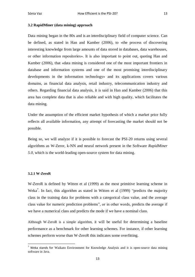
In conclusion, we present the following figure, adapted from Wu, et al. (2008) that
summarizes the k-NN method.
Figure 1: The k-nearest neighbor classification algorithm
3.2.3 Neural Network
According to Han and Kamber (2006), neural networks are, as well as k-NN, «distance-
based mining algorithm» and its name (neural networks) translate on being a set of
interconnected basic units (neurons).
As we can see on Figure 2, which we adapted from Han and Kamber (2006), the
neurons are grouped into three types of layers: input, hidden and output.
Input: D, the set of k training objects, and test object
Process: Compute , the distance between z and every object,
Select , the set of k closest training objects to z.
Output:

Sónia Vaz How Efficient is the PSI-20? 15
15
Figure 2. A multilayer feed-forward neural network
As described by Han and Kamber (2006) and Cabarkapa, et al. (2010), the input layer
receives the input data from external environment and then sends the inputs weighted to
the hidden layer, where the information is processed. Then the outputs of the hidden
layer units can be imputed into another hidden layer (although the most common
procedure is using only one hidden layer) or weighted and sent to the output layer
neurons. In here, the network output will be compared to the desired output resulting on
the network error. Afterward, the network will take this error into account by adjusting
the values of connection weights between the neurons. This process will then be
repeated for a given number of iterations until the network finds the output closest to the
desirable output, which is, in practice, the network output presented to the user.
4. The Data
Our data will be the daily closing values for France, Germany, UK, Greece, Spain and
Portugal stock market indexes8. Then we converted the price series into series of returns
because as mentioned in Brooks (2002) it is preferable to do it like that because, among
other advantages, the use of returns has the added benefit of being unit free. The choice
of these countries is due firstly to compare our results with the ones presented in Borges
(2008, 2010) and secondly because according to International Monetary Fund (2011) all
of these European countries are on the IMF advanced economies list, however France,
8 The stock market indexes are, respectively, CAC 40, DAX 30, FTSE 100, FTSE ATHEX 20, IBEX 35
and PSI 20.
Sónia Vaz How Efficient is the PSI-20? 16
16
Germany and UK stand also in G7 group, being therefore relevant to compare the
results of these countries with the ones of Greece, Spain and Portugal.
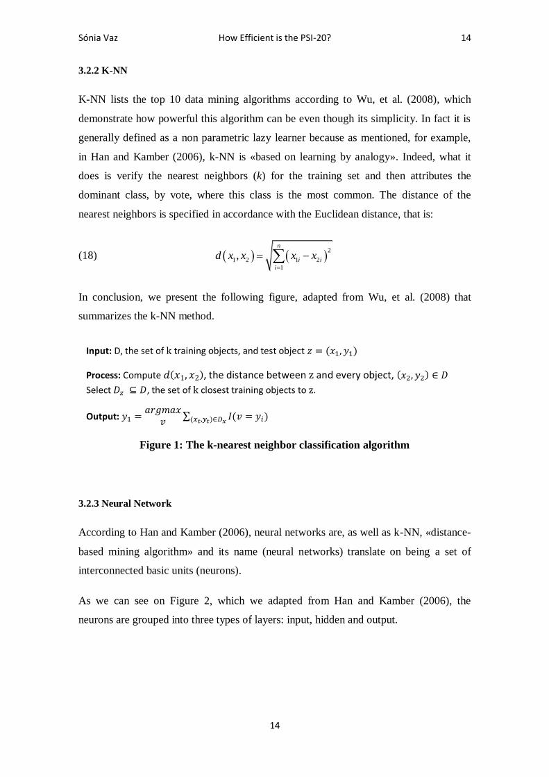
The source of all data is Datastream and the period of analysis is from 01/01/1997 to
31/01/2012. During this period of time, we assist at some financial crisis namely the
April 15th 2000, September 11
th 2001 and more recently the subprime crisis leading
Lehman Brothers to bankruptcy at September 15th
2008.
This way, we will make a cut in the sample at the time of the bankruptcy of
Lehman Brothers, that is, we will apply the empirical tests to a first period from January
1st 1997 to September 12
th 2008 and then compare those results with the ones on the
following period of time: September 15th
2008 to January 31st 2012. In fact, with this,
we intent to show has stated in Lim et al (2008) that after a financial crisis the stock
markets improve their efficiency. It is also important to cover the period from
September 2008 to January 2012 because not only gives an updated approach to this
thesis but also because this period of time was not yet covered by previous studies.
Source: Datastream
Figure 3. Stock Market Indexes - Closing Prices - 1997 to 2012
0
2000
4000
6000
8000
10000
12000
14000
16000
18000
01-0
1-1
997
01-0
1-1
998
01-0
1-1
999
01-0
1-2
000
01-0
1-2
001
01-0
1-2
002
01-0
1-2
003
01-0
1-2
004
01-0
1-2
005
01-0
1-2
006
01-0
1-2
007
01-0
1-2
008
01-0
1-2
009
01-0
1-2
010
01-0
1-2
011
01-0
1-2
012
PSI-20
IBEX 35
FTSE/ATHEX 20
CAC 40
DAX 30
FTSE 100
Sónia Vaz How Efficient is the PSI-20? 17
17
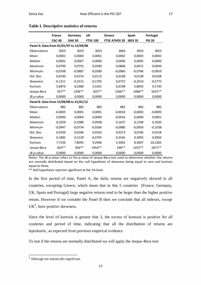
Table I. Descriptive statistics of returns
France Germany UK Greece Spain Portugal
CAC 40 DAX 30 FTSE 100 FTSE ATHEX 20 IBEX 35 PSI 20
Panel A: Data from 01/01/97 to 12/09/08
Observations 3053 3053 3053 2864 3053 3053
Mean 0,0002 0,0003 0,0001 0,0002 0,0003 0,0002
Median 0,0001 0,0007 0,0000 0,0000 0,0005 0,0000
Maximum 0,0700 0,0755 0,0590 0,0868 0,0672 0,0694
Minimum -0,0768 -0,0887 -0,0589 -0,0960 -0,0784 -0,0959
Std. Dev. 0,0140 0,0154 0,0115 0,0168 0,0138 0,0108
Skewness -0,1311 -0,2515 -0,1705 6,0737 -0,2019 -0,5775
Kurtosis 5,6876 6,0380 5,5241 6,6198 5,8693 9,1730
Jarque-Bera 927** 1206** 825** 1566** 1068** 5015**
JB p-value 0,0000 0,0000 0,0000 0,0000 0,0000 0,0000
Panel B: Data from 15/09/08 to 31/01/12
Observations 882 882 882 882 882 882
Mean -0,0003 0,0001 0,0001 -0,0018 -0,0003 -0,0005
Median 0,0000 0,0004 0,0000 -0,0016 0,0000 0,0001
Maximum 0,1059 0,1080 0,0938 0,1637 0,1348 0,1020
Minimum -0,0947 -0,0734 -0,9266 -0,0980 -0,0959 -0,1038
Std. Dev. 0,0194 0,0186 0,0162 0,0273 0,0196 0,0158
Skewness 0,1882 0,2139 -0,0795 0,3545 0,3093 0,0950
Kurtosis 7,7236 7,8095 9,2906 5,5002 8,3697 10,1365
Jarque-Bera 824** 856** 1454** 248** 1072** 1871**
JB p-value 0,0000 0,0000 0,0000 0,0000 0,0000 0,0000
Notes: The JB p-value refers to the p-value of Jarque-Bera test used to determine whether the returns are normally distributed based on the null hypothesis of skewness being equal to zero and kurtosis equal to three. ** Null hypothesis rejection significant at the 1% level.
In the first period of time, Panel A, the daily returns are negatively skewed in all
countries, excepting Greece, which mean that in this 5 countries (France, Germany,
UK, Spain and Portugal) large negative returns tend to be larger than the higher positive
retuns. However if we consider the Panel B then we conclude that all indexes, except
UK9, have positive skewness.
Since the level of kurtosis is greater that 3, the excess of kurtosis is positive for all
countries and period of time, indicating that all the distribution of returns are
leptokurtic, as expected from previous empirical evidence.
To test if the returns are normally distributed we will apply the Jarque-Bera test:
9 Although not statistically significant.

Sónia Vaz How Efficient is the PSI-20? 18
18
(19) 2 2
2
(2)
( 3)
6 24
ks kJB n
where sk means skewness and k kurtosis.
being the null hypothesis:
H0: normal distribution,
skewness is zero and kurtosis is three.
H1: non-normal distribution
As presented at Table I, the JB p-value are all very close to zero, which implies that the
null hypothesis is strongly rejected for any usual level for every stock market index for
both periods, and therefore stock market indexes’ returns are not normally distributed.
It is also necessary to mention that in Appendix A1 and A2 there are the comparison
with the histograms of the stock indexes’ returns and the Normal Distribution for the
corresponding period of time.
5. Results
In this chapter we will present the results on the tests referred in the Methodology.
Additionally we will present a table that summarizes the results of the performed
classical efficiency tests, answering the question “Is the random walk hypothesis
rejected?” for each one.
5.1 Classical Efficiency tests
5.1.1 Correlations
The results for the tests on autocorrelation, partial correlation and Ljung-Box Q-statistic
probability are expressed on Table II.
Sónia Vaz How Efficient is the PSI-20? 19
19
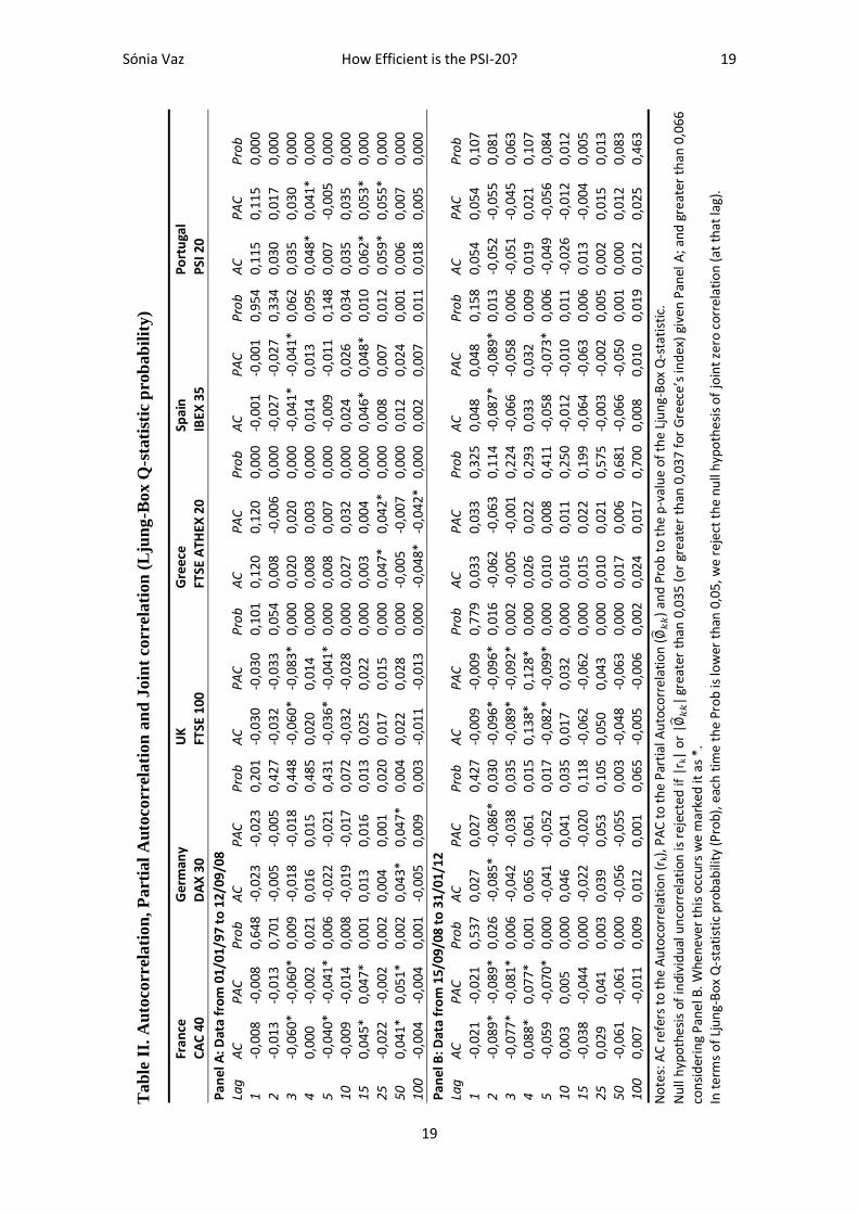
Tab
le I
I. A
uto
corr
elati
on
, P
art
ial
Au
tocorr
elati
on
an
d J
oin
t co
rrel
ati
on
(L
jun
g-B
ox Q
-sta
tist
ic p
rob
ab
ilit
y)
Fr
an
ce
Ge
rman
y U
K
Gre
ece
Spai
n
Po
rtu
gal
C
AC
40
D
AX
30
FTSE
100
FT
SE A
THEX
20
IBEX
35
PSI
20
Pa
nel
A: D
ata
fro
m 0
1/0
1/97
to
12/
09/0
8 La
g
AC
P
AC
P
rob
A
C
PA
C
Pro
b
AC
P
AC
P
rob
A
C
PA
C
Pro
b
AC
P
AC
P
rob
A
C
PA
C
Pro
b
1
-0,0
08
-0
,00
8
0,64
8
-0,0
23
-0,0
23
0,
201
-0
,030
-0
,030
0,
101
0,
120
0,
120
0,
000
-0
,001
-0
,001
0,
954
0,
115
0,
115
0,
000
2
-0,0
13
-0
,01
3
0,70
1
-0,0
05
-0,0
05
0,
427
-0
,032
-0
,033
0,
054
0,
008
-0
,00
6 0,
000
-0
,027
-0
,027
0,
334
0,
030
0,
017
0,
000
3
-0
,06
0*
-0,0
60*
0,
009
-0
,018
-0
,01
8
0,44
8
-0,0
60*
-0,0
83*
0,00
0
0,02
0
0,02
0
0,00
0
-0,0
41*
-0,0
41*
0,06
2
0,03
5
0,03
0
0,00
0
4
0,0
00
-0
,00
2
0,02
1
0,01
6
0,0
15
0,48
5
0,02
0
0,01
4
0,00
0
0,00
8
0,00
3
0,00
0
0,01
4
0,01
3
0,09
5
0,04
8*
0,04
1*
0,00
0
5
-0,0
40*
-0
,04
1*
0,00
6
-0,0
22
-0,0
21
0,
431
-0
,036
* -0
,041
* 0,
000
0,
008
0,
007
0,
000
-0
,009
-0
,011
0,
148
0,
007
-0
,005
0,
000
10
-0
,00
9
-0,0
14
0,
008
-0
,019
-0
,01
7
0,07
2
-0,0
32
-0,0
28
0,00
0
0,02
7
0,03
2
0,00
0
0,02
4
0,02
6
0,03
4
0,03
5
0,03
5
0,00
0
15
0,0
45*
0,
047*
0,
001
0,
013
0,
016
0,
013
0,
025
0,
022
0,
000
0,
003
0,
004
0,
000
0,
046*
0,
048*
0,
010
0,
062*
0,
053*
0,
000
25
-0,0
22
-0
,00
2
0,00
2
0,00
4
0,0
01
0,02
0
0,01
7
0,01
5
0,00
0
0,04
7*
0,04
2*
0,00
0
0,00
8
0,00
7
0,01
2
0,05
9*
0,05
5*
0,00
0
50
0,0
41*
0,
05
1*
0,00
2
0,04
3*
0,
047
*
0,00
4
0,02
2
0,02
8
0,00
0
-0,0
05
-0,0
07
0,00
0
0,01
2
0,02
4
0,00
1
0,00
6
0,00
7
0,00
0
100
-0
,00
4
-0,0
04
0,
001
-0
,005
0,
009
0,
003
-0
,011
-0
,013
0,
000
-0
,048
* -0
,042
* 0,
000
0,
002
0,
007
0,
011
0,
018
0,
005
0,
000
Pa
nel
B: D
ata
fro
m 1
5/0
9/08
to
31/
01/
12
Lag
A
C
PA
C
Pro
b
AC
P
AC
P
rob
A
C
PA
C
Pro
b
AC
P
AC
P
rob
A
C
PA
C
Pro
b
AC
P
AC
P
rob
1
-0,0
21
-0
,02
1
0,53
7
0,02
7
0,0
27
0,42
7
-0,0
09
-0,0
09
0,77
9
0,03
3
0,03
3
0,32
5
0,04
8
0,04
8
0,15
8
0,05
4
0,05
4
0,10
7
2
-0,0
89*
-0
,08
9*
0,02
6
-0,0
85*
-0,0
86*
0,
030
-0
,096
* -0
,096
* 0,
016
-0
,062
-0
,063
0,
114
-0
,087
* -0
,089
* 0,
013
-0
,052
-0
,055
0,
081
3
-0
,07
7*
-0,0
81*
0,
006
-0
,042
-0
,03
8
0,03
5
-0,0
89*
-0,0
92*
0,00
2
-0,0
05
-0,0
01
0,22
4
-0,0
66
-0,0
58
0,00
6
-0,0
51
-0,0
45
0,06
3
4
0,0
88*
0,
077*
0,
001
0,
065
0,
061
0,
015
0,
138*
0,
128*
0,
000
0,
026
0,
022
0,
293
0,
033
0,
032
0,
009
0,
019
0,
021
0,
107
5
-0
,05
9
-0,0
70*
0,
000
-0
,041
-0
,05
2
0,01
7
-0,0
82*
-0,0
99*
0,00
0
0,01
0
0,00
8
0,41
1
-0,0
58
-0,0
73*
0,00
6
-0,0
49
-0,0
56
0,08
4
10
0,0
03
0,
005
0,
000
0,
046
0,
041
0,
035
0,
017
0,
032
0,
000
0,
016
0,
011
0,
250
-0
,012
-0
,010
0,
011
-0
,026
-0
,012
0,
012
15
-0,0
38
-0
,04
4
0,00
0
-0,0
22
-0,0
20
0,
118
-0
,062
-0
,062
0,
000
0,
015
0,
022
0,
199
-0
,064
-0
,063
0,
006
0,
013
-0
,004
0,
005
25
0
,02
9
0,04
1
0,00
3
0,03
9
0,0
53
0,10
5
0,05
0
0,04
3
0,00
0
0,01
0
0,02
1
0,57
5
-0,0
03
-0,0
02
0,00
5
0,00
2
0,01
5
0,01
3
50
-0,0
61
-0
,06
1
0,00
0
-0,0
56
-0,0
55
0,
003
-0
,048
-0
,063
0,
000
0,
017
0,
006
0,
681
-0
,066
-0
,050
0,
001
0,
000
0,
012
0,
083
10
0
0,0
07
-0
,01
1
0,00
9
0,01
2
0,0
01
0,06
5
-0,0
05
-0,0
06
0,00
2
0,02
4
0,01
7
0,70
0
0,00
8
0,01
0
0,01
9
0,01
2
0,02
5
0,46
3
No
tes:
AC
ref
ers
to t
he
Au
toco
rrel
atio
n (
r k),
PA
C t
o th
e P
arti
al A
uto
corr
elat
ion
(
) an
d P
rob
to
the
p-v
alu
e o
f th
e Lj
un
g-B
ox Q
-sta
tist
ic.
Nu
ll h
ypo
thes
is o
f in
divi
du
al u
nco
rrel
atio
n is
rej
ecte
d if
|r k
| o
r |
grea
ter
than
0,0
35 (
or
grea
ter
than
0,0
37 f
or G
reec
e’s
ind
ex)
give
n P
anel
A; a
nd
grea
ter
than
0,0
66
con
sid
erin
g P
anel
B. W
hen
ever
th
is o
ccur
s w
e m
arke
d it
as
*.
In t
erm
s o
f Lj
un
g-B
ox
Q-s
tati
stic
pro
bab
ility
(P
rob
), e
ach
tim
e th
e Pr
ob
is lo
wer
th
an 0
,05,
we
reje
ct t
he
nu
ll h
ypo
thes
is o
f jo
int
zero
cor
rela
tio
n (
at t
hat
lag)
.
Sónia Vaz How Efficient is the PSI-20? 20
20
Recall that if
then the null hypothesis that the true value of the
coefficient at lag k is zero is rejected. This means that, for the first period, the critical
value is 0,035 for all countries except Greece, which is 0,037 and for the second period,
the critical value is 0,066 for all market indexes10
.
Given the Panel A of Table II, the null hypothesis of joint zero correlation in France is
rejected as from lag 3, in Germany as from lag 15 and in UK as from lag 3. There are
also some evidence of correlation (AC and PAC) in France at lags 3, 5, 15 and 50; in
Germany at lag 50 and in UK at lags 3 and 5. We can also conclude that we reject the
null hypothesis of joint zero correlation for all lags in Greece and Portugal. Cosidering
Spain, there are evidence of joint zero correlation of returns in the first lags, however
from lag 10 there are evidence of joint correlation.
Observing the Panel B, at lag 100, the joint zero correlation is rejected for CAC 40,
FTSE 100 and IBEX 35.
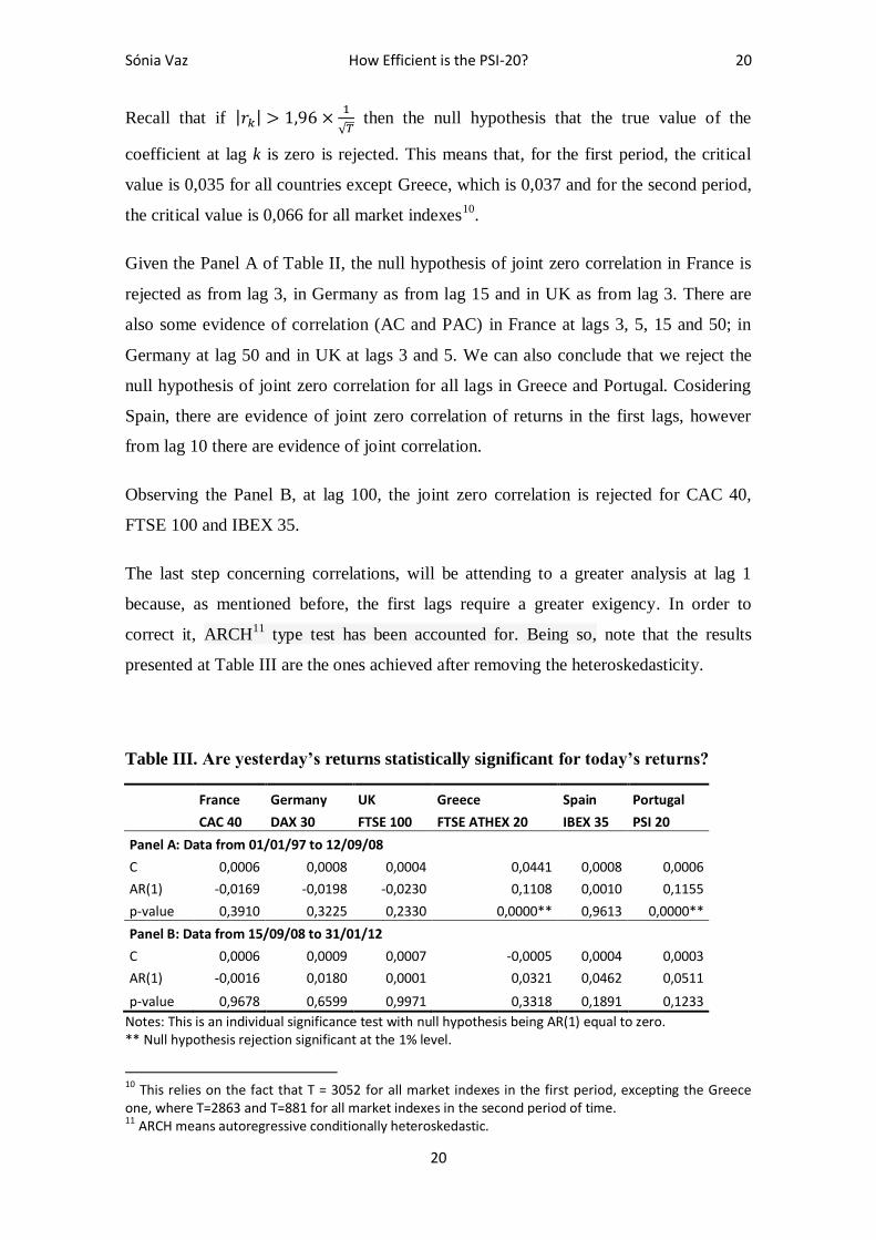
The last step concerning correlations, will be attending to a greater analysis at lag 1
because, as mentioned before, the first lags require a greater exigency. In order to
correct it, ARCH11
type test has been accounted for. Being so, note that the results
presented at Table III are the ones achieved after removing the heteroskedasticity.
Table III. Are yesterday’s returns statistically significant for today’s returns?
France Germany UK Greece Spain Portugal
CAC 40 DAX 30 FTSE 100 FTSE ATHEX 20 IBEX 35 PSI 20
Panel A: Data from 01/01/97 to 12/09/08
C 0,0006 0,0008 0,0004 0,0441 0,0008 0,0006
AR(1) -0,0169 -0,0198 -0,0230 0,1108 0,0010 0,1155
p-value 0,3910 0,3225 0,2330 0,0000** 0,9613 0,0000**
Panel B: Data from 15/09/08 to 31/01/12
C 0,0006 0,0009 0,0007 -0,0005 0,0004 0,0003
AR(1) -0,0016 0,0180 0,0001 0,0321 0,0462 0,0511
p-value 0,9678 0,6599 0,9971 0,3318 0,1891 0,1233
Notes: This is an individual significance test with null hypothesis being AR(1) equal to zero. ** Null hypothesis rejection significant at the 1% level.
10
This relies on the fact that T = 3052 for all market indexes in the first period, excepting the Greece one, where T=2863 and T=881 for all market indexes in the second period of time. 11 ARCH means autoregressive conditionally heteroskedastic.
Sónia Vaz How Efficient is the PSI-20? 21
21
As we have seen previously in the correlograms and now on table III, yesterday’s
returns were only statiscally significant for today’s returns in Greece and Portugal for
the first period of time (Panel A). However, for the second period of time, Panel B, all
indexes show that there are no correlation at lag 1.
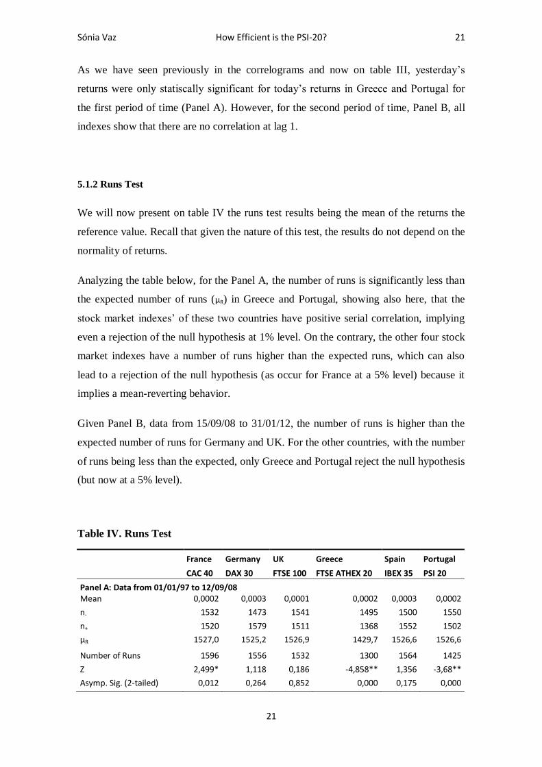
5.1.2 Runs Test
We will now present on table IV the runs test results being the mean of the returns the
reference value. Recall that given the nature of this test, the results do not depend on the
normality of returns.
Analyzing the table below, for the Panel A, the number of runs is significantly less than
the expected number of runs (µR) in Greece and Portugal, showing also here, that the
stock market indexes’ of these two countries have positive serial correlation, implying
even a rejection of the null hypothesis at 1% level. On the contrary, the other four stock
market indexes have a number of runs higher than the expected runs, which can also
lead to a rejection of the null hypothesis (as occur for France at a 5% level) because it
implies a mean-reverting behavior.
Given Panel B, data from 15/09/08 to 31/01/12, the number of runs is higher than the
expected number of runs for Germany and UK. For the other countries, with the number
of runs being less than the expected, only Greece and Portugal reject the null hypothesis
(but now at a 5% level).
Table IV. Runs Test
France Germany UK Greece Spain Portugal
CAC 40 DAX 30 FTSE 100 FTSE ATHEX 20 IBEX 35 PSI 20
Panel A: Data from 01/01/97 to 12/09/08 Mean 0,0002 0,0003 0,0001 0,0002 0,0003 0,0002
n- 1532 1473 1541 1495 1500 1550
n+ 1520 1579 1511 1368 1552 1502
µR 1527,0 1525,2 1526,9 1429,7 1526,6 1526,6
Number of Runs 1596 1556 1532 1300 1564 1425
Z 2,499* 1,118 0,186 -4,858** 1,356 -3,68**
Asymp. Sig. (2-tailed) 0,012 0,264 0,852 0,000 0,175 0,000
Sónia Vaz How Efficient is the PSI-20? 22
22
Panel B: Data from 15/09/08 to 31/01/12 Mean -0,0003 0,0001 0,0001 -0,0018 -0,0003 -0,0005
n- 428 434 443 431 414 413
n+ 453 447 438 450 467 468
µR 441,1 441,4 441,5 441,3 439,9 439,8
Number of Runs 424 442 450 406 416 403
Z -1,157 0,04 0,574 -2,381* -1,618 -2,49*
Asymp. Sig. (2-tailed) 0,247 0,968 0,566 0,017 0,106 0,013
Notes: We tested as test value the mean of the stock indexes’ returns. The runs test assumes as a null hypothesis the elements of the series are mutually independent. * Null hypotehsis rejection significant at the 5% level. ** Null hypothesis rejection significant at the 1% level.
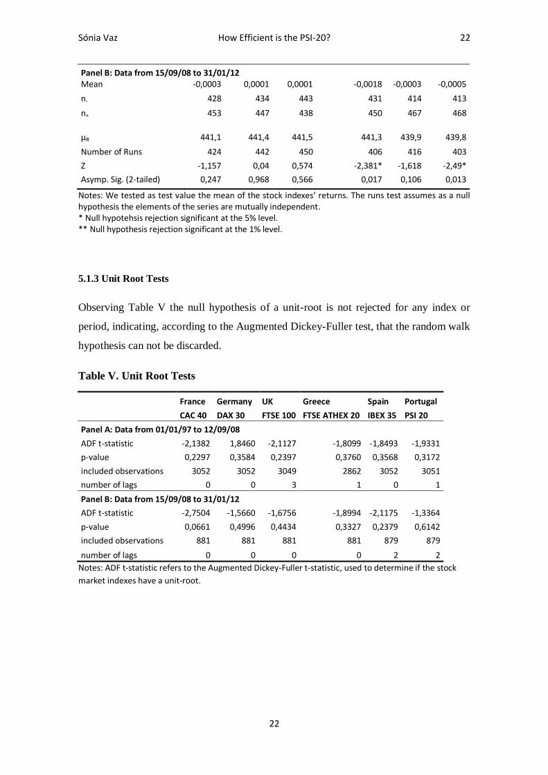
5.1.3 Unit Root Tests
Observing Table V the null hypothesis of a unit-root is not rejected for any index or
period, indicating, according to the Augmented Dickey-Fuller test, that the random walk
hypothesis can not be discarded.
Table V. Unit Root Tests
France Germany UK Greece Spain Portugal
CAC 40 DAX 30 FTSE 100 FTSE ATHEX 20 IBEX 35 PSI 20
Panel A: Data from 01/01/97 to 12/09/08
ADF t-statistic -2,1382 1,8460 -2,1127 -1,8099 -1,8493 -1,9331
p-value 0,2297 0,3584 0,2397 0,3760 0,3568 0,3172
included observations 3052 3052 3049 2862 3052 3051
number of lags 0 0 3 1 0 1
Panel B: Data from 15/09/08 to 31/01/12
ADF t-statistic -2,7504 -1,5660 -1,6756 -1,8994 -2,1175 -1,3364
p-value 0,0661 0,4996 0,4434 0,3327 0,2379 0,6142
included observations 881 881 881 881 879 879
number of lags 0 0 0 0 2 2
Notes: ADF t-statistic refers to the Augmented Dickey-Fuller t-statistic, used to determine if the stock
market indexes have a unit-root.

Sónia Vaz How Efficient is the PSI-20? 23
23
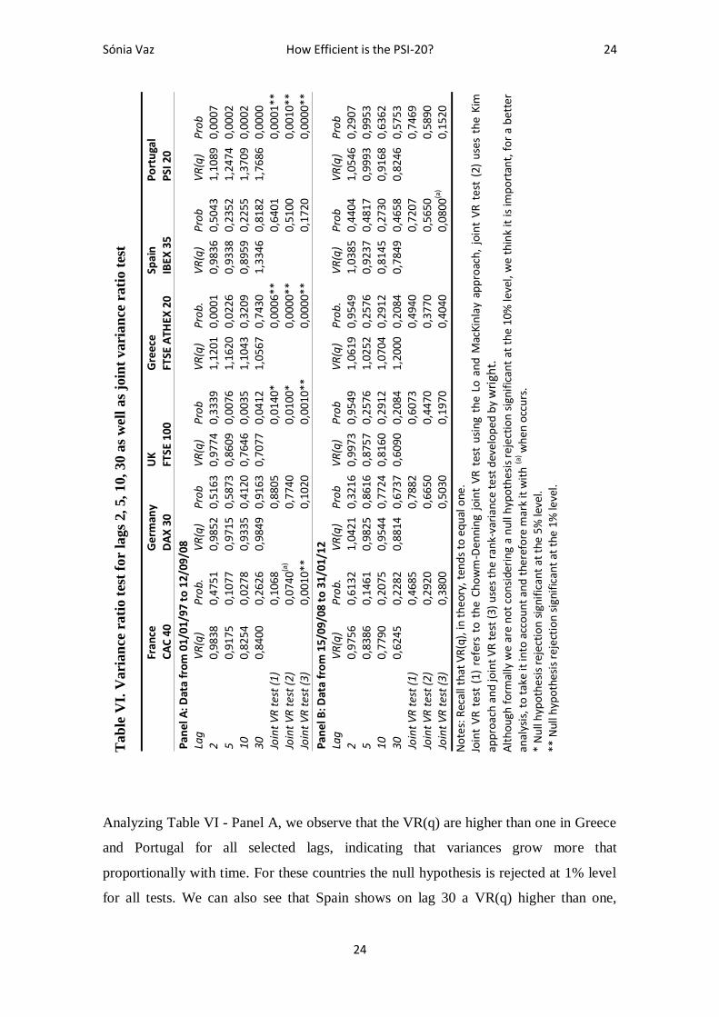
5.1.4 Variance Ratio Tests
Our fourth test is the Variance Ratio (VR) test, which according Lo and MacKinlay
(1989), provides an added advantage because is a more reliable test than testing for
correlations or unit roots.
For VR test we will present three approaches: the first is VR test robust under
heteroskedasticity proposed by Lo and MacKinlay (1988); the second approach is the
wild bootstrap sugested by Kim (2006); and the third approach is the VR test based on
ranks and signs12
, as proposed by Wright (2000).
In order to facilitate comparisons with other recent studies, we selected the lags 2, 5, 10
and 30.
12
Although Wright’s methodology proposes two alternatives: a rank test and a sign test, in this thesis we chose to perform the rank VR test.
Sónia Vaz How Efficient is the PSI-20? 24
24
Analyzing Table VI - Panel A, we observe that the VR(q) are higher than one in Greece
and Portugal for all selected lags, indicating that variances grow more that
proportionally with time. For these countries the null hypothesis is rejected at 1% level
for all tests. We can also see that Spain shows on lag 30 a VR(q) higher than one,
Tab
le V
I. V
ari
an
ce r
ati
o t
est
for
lags
2,
5,
10,
30 a
s w
ell
as
join
t vari
an
ce r
ati
o t
est
Fr
an
ce
Ger
man
y U
K
Gre
ece
Spai
n
Po
rtu
gal
C
AC
40
D
AX
30
FTSE
100
FT
SE A
THEX
20
IBEX
35
PSI
20
Pan
el A
: Dat
a fr
om
01
/01/
97 t
o 1
2/09
/08
Lag
V
R(q
) P
rob.
V
R(q
) P
rob
V
R(q
) P
rob
V
R(q
) P
rob.
V
R(q
) P
rob
V
R(q
) P
rob
2
0,9
838
0,
4751
0,
9852
0,
5163
0,
9774
0,
3339
1,
1201
0,
0001
0,
9836
0,
5043
1,
1089
0,
0007
5 0
,917
5
0,10
77
0,97
15
0,58
73
0,86
09
0,00
76
1,16
20
0,02
26
0,93
38
0,23
52
1,24
74
0,00
02
10
0,8
254
0,
0278
0,
9335
0,
4120
0,
7646
0,
0035
1,
1043
0,
3209
0,
8959
0,
2255
1,
3709
0,
0002
30
0
,840
0
0,26
26
0,98
49
0,91
63
0,70
77
0,04
12
1,05
67
0,74
30
1,33
46
0,81
82
1,76
86
0,00
00
Join
t V
R t
est
(1)
0,
1068
0,88
05
0,
0140
*
0,
0006
**
0,
6401
0,00
01**
Jo
int
VR
tes
t (2
)
0,07
40(a
)
0,77
40
0,
0100
*
0,
0000
**
0,
5100
0,00
10**
Jo
int
VR
tes
t (3
)
0,00
10**
0,10
20
0,
0010
**
0,
0000
**
0,
1720
0,00
00**
Pan
el B
: Dat
a fr
om
15/
09/0
8 to
31/
01/1
2
Lag
V
R(q
) P
rob.
V
R(q
) P
rob
V
R(q
) P
rob
V
R(q
) P
rob.
V
R(q
) P
rob
V
R(q
) P
rob
2
0,9
756
0,
6132
1,
0421
0,
3216
0,
9973
0,
9549
1,
0619
0,
9549
1,
0385
0,
4404
1,
0546
0,
2907
5
0,8
386
0,
1461
0,
9825
0,
8616
0,
8757
0,
2576
1,
0252
0,
2576
0,
9237
0,
4817
0,
9993
0,
9953
10
0
,779
0
0,20
75
0,95
44
0,77
24
0,81
60
0,29
12
1,07
04
0,29
12
0,81
45
0,27
30
0,91
68
0,63
62
30
0,6
245
0,
2282
0,
8814
0,
6737
0,
6090
0,
2084
1,
2000
0,
2084
0,
7849
0,
4658
0,
8246
0,
5753
Jo
int
VR
tes
t (1
)
0,46
85
0,
7882
0,60
73
0,
4940
0,72
07
0,
7469
Jo
int
VR
tes
t (2
)
0,29
20
0,
6650
0,44
70
0,
3770
0,56
50
0,
5890
Jo
int
VR
tes
t (3
)
0,38
00
0,
5030
0,19
70
0,
4040
0,08
00(a
)
0,15
20
No
tes:
Rec
all t
hat
VR
(q),
in t
heo
ry, t
end
s to
eq
ual
one
. Jo
int
VR
tes
t (1
) re
fers
to
th
e C
ho
wm
-Den
nin
g jo
int
VR
tes
t u
sin
g th
e Lo
an
d M
acKi
nla
y ap
pro
ach
, jo
int
VR
tes
t (2
) u
ses
the
Kim
app
roac
h a
nd
join
t V
R t
est
(3)
use
s th
e ra
nk-
vari
ance
tes
t d
evel
op
ed b
y w
righ
t.
Alt
ho
ugh
fo
rmal
ly w
e ar
e n
ot
con
side
rin
g a
nul
l hyp
oth
esis
rej
ecti
on
sign
ific
ant
at t
he
10%
leve
l, w
e th
ink
it is
imp
ort
ant,
fo
r a
bet
ter
anal
ysis
, to
tak
e it
into
acc
ou
nt
and
the
refo
re m
ark
it w
ith
(a) w
hen
occ
urs
. *
Nu
ll h
ypo
thes
is r
ejec
tio
n s
igni
fica
nt
at t
he 5
% le
vel.
** N
ull
hyp
oth
esis
rej
ect
ion
sig
nifi
can
t at
the
1%
leve
l.
Sónia Vaz How Efficient is the PSI-20? 25
25
however this event is not statistically relevant and the null hypothesis is not rejected for
any of the three tests. In Germany the null hypothesis is also not rejected for any of the
joint VR test. Regarding UK, the null hypothesis of the joint VR test is rejected at a 5%
level for the Lo and MacKinlay approach as well as for the Kim approach, in addition to
a rejection at 1% level for the Wright approach. At last, France shows no rejection in
terms of the joint VR test concerning the Lo and MacKinlay approach but in terms of
the Kim approach already demonstrate some possibility of rejection (null hypothesis
rejection significant at the 10% level), leading to a rejection at 5% level when
considering the Wright approach (recall that this test can be more robust than the other).
Analyzing the Panel B, we can see some improvements in terms of market efficiency
because there is no rejection (at 1% and 5% level) of the null hypothesis for any stock
market index. However it is important to point that for Wright approach in Spain, the
null hypothesis could be rejected at a 10% level.
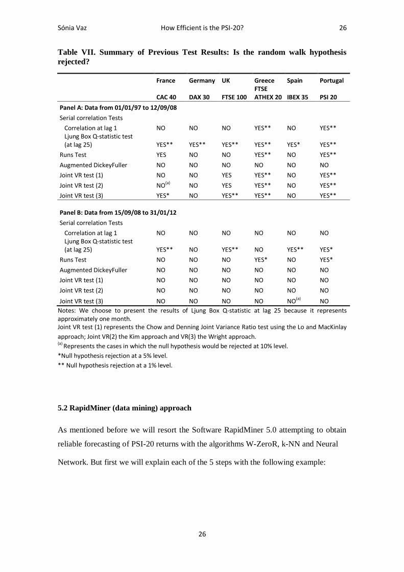
5.1.5 Summary of Tests Results
In the Table VII we summarized the previous test results, where it is clear that all stock
market indexes, excepting Spain, improved their efficiency after the financial crisis.
Analyzing Panel A, we achieved similar conclusions to the ones in Borges (2008, 2010)
and report that the random hypothesis is rejected, in every test excepting the ADF, for
both FTSE ATHEX 20 and PSI 20. Regarding Panel B (the period not yet covered by
previous studies) this hypothesis is now only rejected for the Runs test concerning
Greece’s index; and for the Ljung Box Q-statistic test and Runs Test concerning
Portugal’s index. It is also worth mentioning that, for the Panel B, the random walk
hypothesis is not rejected for any test regarding DAX 30 index.
As for the IBEX 35, the only index that did not improved its efficiency, although in
Panel A it is apparently the best (random walk only rejected at a 5% level for the Ljung
Box Q-statistic), given Panel B, for the Ljung Box Q-statistic the random walk is now
rejected at a 1% level and if we want to be thorough, we can also refer that the random
walk can be rejected at a 10% level concerning the Wright VR test.
Sónia Vaz How Efficient is the PSI-20? 26
26
Table VII. Summary of Previous Test Results: Is the random walk hypothesis
rejected?
France Germany UK Greece Spain Portugal
CAC 40 DAX 30 FTSE 100 FTSE ATHEX 20 IBEX 35 PSI 20
Panel A: Data from 01/01/97 to 12/09/08
Serial correlation Tests Correlation at lag 1 NO NO NO YES** NO YES**
Ljung Box Q-statistic test (at lag 25) YES** YES** YES** YES** YES* YES**
Runs Test YES NO NO YES** NO YES**
Augmented DickeyFuller NO NO NO NO NO NO
Joint VR test (1) NO NO YES YES** NO YES**
Joint VR test (2) NO(a) NO YES YES** NO YES**
Joint VR test (3) YES* NO YES** YES** NO YES**
Panel B: Data from 15/09/08 to 31/01/12
Serial correlation Tests Correlation at lag 1 NO NO NO NO NO NO
Ljung Box Q-statistic test (at lag 25) YES** NO YES** NO YES** YES*
Runs Test NO NO NO YES* NO YES*
Augmented DickeyFuller NO NO NO NO NO NO
Joint VR test (1) NO NO NO NO NO NO
Joint VR test (2) NO NO NO NO NO NO
Joint VR test (3) NO NO NO NO NO(a) NO
Notes: We choose to present the results of Ljung Box Q-statistic at lag 25 because it represents approximately one month. Joint VR test (1) represents the Chow and Denning Joint Variance Ratio test using the Lo and MacKinlay
approach; Joint VR(2) the Kim approach and VR(3) the Wright approach. (a) Represents the cases in which the null hypothesis would be rejected at 10% level.
*Null hypothesis rejection at a 5% level.
** Null hypothesis rejection at a 1% level.
5.2 RapidMiner (data mining) approach
As mentioned before we will resort the Software RapidMiner 5.0 attempting to obtain
reliable forecasting of PSI-20 returns with the algorithms W-ZeroR, k-NN and Neural
Network. But first we will explain each of the 5 steps with the following example:
Sónia Vaz How Efficient is the PSI-20? 27
27
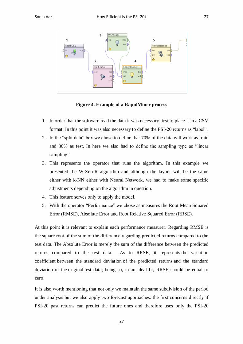
Figure 4. Example of a RapidMiner process
1. In order that the software read the data it was necessary first to place it in a CSV
format. In this point it was also necessary to define the PSI-20 returns as “label”.
2. In the “split data” box we chose to define that 70% of the data will work as train
and 30% as test. In here we also had to define the sampling type as “linear
sampling”
3. This represents the operator that runs the algorithm. In this example we
presented the W-ZeroR algorithm and although the layout will be the same
either with k-NN either with Neural Network, we had to make some specific
adjustments depending on the algorithm in question.
4. This feature serves only to apply the model.
5. With the operator “Performance” we chose as measures the Root Mean Squared
Error (RMSE), Absolute Error and Root Relative Squared Error (RRSE).
At this point it is relevant to explain each performance measurer. Regarding RMSE is
the square root of the sum of the difference regarding predicted returns compared to the
test data. The Absolute Error is merely the sum of the difference between the predicted
returns compared to the test data. As to RRSE, it represents the variation
coefficient between the standard deviation of the predicted returns and the standard
deviation of the original test data; being so, in an ideal fit, RRSE should be equal to
zero.
It is also worth mentioning that not only we maintain the same subdivision of the period
under analysis but we also apply two forecast approaches: the first concerns directly if
PSI-20 past returns can predict the future ones and therefore uses only the PSI-20
1
2
3
4
5

Sónia Vaz How Efficient is the PSI-20? 28
28
returns as inputs; for the second approach we aggregate the returns into 4 classes (class
1 for returns lower than -5%, class 2 for returns between -5% and zero, class 3 for
returns between zero and 5% and class 4 for returns greater than 5%).
In the next sub-chapters we will present the results of forecasting with the three chosen
algorithms (W-Zeror, k-NN and Neural Network) for each period of time and taking
into account the two approaches mentioned above.
Additionally we will also present a strategy that we design and implement using the best
estimates of the k-NN and the Neural Net to find out if we can obtain greater results
than the ones achieved using a buy and hold strategy.
5.2.1 W-ZeroR
As mentioned before, the W-ZeroR has in here the purpose of give us a forecasting
benchmark. Being so is expected that the k-NN and the Neural Network have lower
RMSE, absolute error and RRSE than the ones presented on Table VIII.
Table VIII. Performance of the algorithm W-ZeroR
Root Mean Squared Error Absolute Error Root Relative Squared Error
Panel A: Results using only the PSI-20 returns as inputs with data from 01/01/97 to 12/09/08
0,009 0,006 +/- 0,007 1,000
Panel B: Results aggregating the PSI-20 returns in classes with data from 01/01/97 to 12/09/08
0,009 0,006 +/- 0,007 1,000
Panel C: Results using only the PSI-20 returns as inputs with data from 15/09/08 to 31/01/12
0,014 0,011 +/- 0,009 1,004
Panel D: Results aggregating the PSI-20 returns in classes with data from 15/09/08 to 31/01/12
0,014 0,011 +/- 0,009 1,004
Since W-ZeroR predicts the average of a numerical series, and the mean of the PSI-20
returns is approximately 0%, aggregating the PSI-20 returns in classes does not
translate, in here, in an evident advantage. Also, is without surprise that we achieve the
following forecasting results:
Sónia Vaz How Efficient is the PSI-20? 29
29
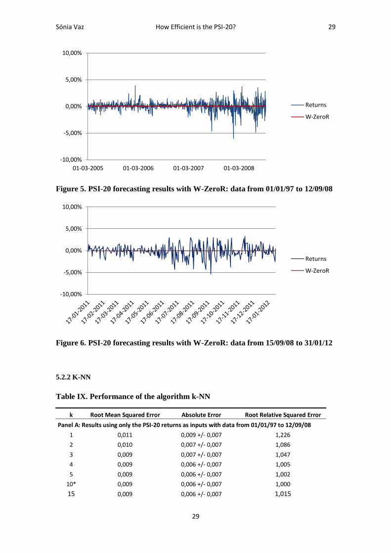
Figure 5. PSI-20 forecasting results with W-ZeroR: data from 01/01/97 to 12/09/08
Figure 6. PSI-20 forecasting results with W-ZeroR: data from 15/09/08 to 31/01/12
5.2.2 K-NN
Table IX. Performance of the algorithm k-NN
k Root Mean Squared Error Absolute Error Root Relative Squared Error
Panel A: Results using only the PSI-20 returns as inputs with data from 01/01/97 to 12/09/08
1 0,011 0,009 +/- 0,007 1,226
2 0,010 0,007 +/- 0,007 1,086
3 0,009 0,007 +/- 0,007 1,047
4 0,009 0,006 +/- 0,007 1,005
5 0,009 0,006 +/- 0,007 1,002
10* 0,009 0,006 +/- 0,007 1,000
15 0,009 0,006 +/- 0,007 1,015
-10,00%
-5,00%
0,00%
5,00%
10,00%
01-03-2005 01-03-2006 01-03-2007 01-03-2008
Returns
W-ZeroR
-10,00%
-5,00%
0,00%
5,00%
10,00%
Returns
W-ZeroR
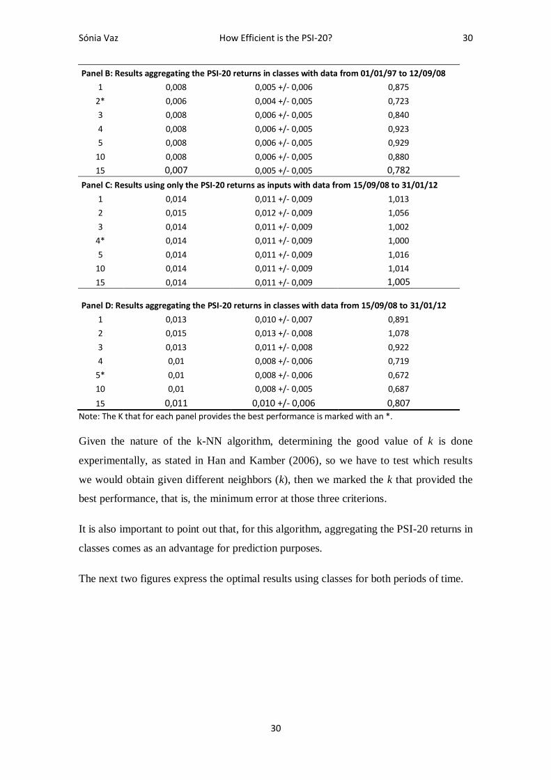
Sónia Vaz How Efficient is the PSI-20? 30
30
Panel B: Results aggregating the PSI-20 returns in classes with data from 01/01/97 to 12/09/08
1 0,008 0,005 +/- 0,006 0,875
2* 0,006 0,004 +/- 0,005 0,723
3 0,008 0,006 +/- 0,005 0,840
4 0,008 0,006 +/- 0,005 0,923
5 0,008 0,006 +/- 0,005 0,929
10 0,008 0,006 +/- 0,005 0,880
15 0,007 0,005 +/- 0,005 0,782
Panel C: Results using only the PSI-20 returns as inputs with data from 15/09/08 to 31/01/12
1 0,014 0,011 +/- 0,009 1,013
2 0,015 0,012 +/- 0,009 1,056
3 0,014 0,011 +/- 0,009 1,002
4* 0,014 0,011 +/- 0,009 1,000
5 0,014 0,011 +/- 0,009 1,016
10 0,014 0,011 +/- 0,009 1,014
15 0,014 0,011 +/- 0,009 1,005 Panel D: Results aggregating the PSI-20 returns in classes with data from 15/09/08 to 31/01/12
1 0,013 0,010 +/- 0,007 0,891
2 0,015 0,013 +/- 0,008 1,078
3 0,013 0,011 +/- 0,008 0,922
4 0,01 0,008 +/- 0,006 0,719
5* 0,01 0,008 +/- 0,006 0,672
10 0,01 0,008 +/- 0,005 0,687
15 0,011 0,010 +/- 0,006 0,807
Note: The K that for each panel provides the best performance is marked with an *.
Given the nature of the k-NN algorithm, determining the good value of k is done
experimentally, as stated in Han and Kamber (2006), so we have to test which results
we would obtain given different neighbors (k), then we marked the k that provided the
best performance, that is, the minimum error at those three criterions.
It is also important to point out that, for this algorithm, aggregating the PSI-20 returns in
classes comes as an advantage for prediction purposes.
The next two figures express the optimal results using classes for both periods of time.
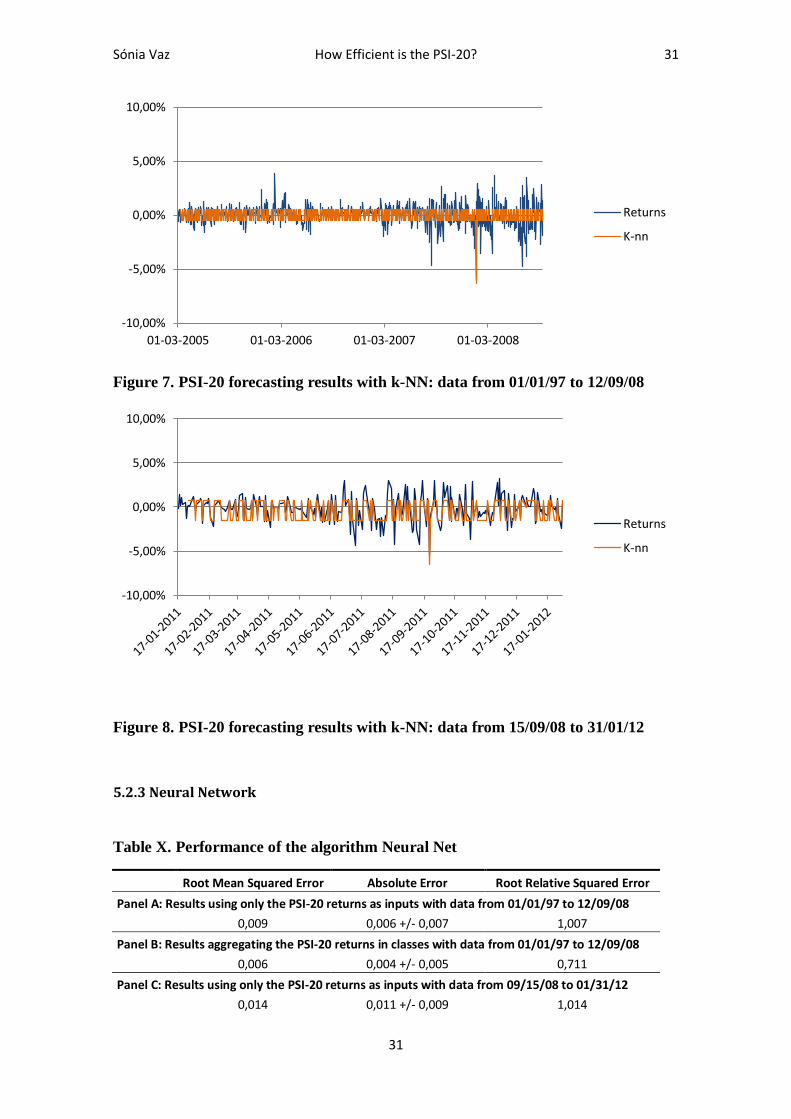
Sónia Vaz How Efficient is the PSI-20? 31
31
Figure 7. PSI-20 forecasting results with k-NN: data from 01/01/97 to 12/09/08
Figure 8. PSI-20 forecasting results with k-NN: data from 15/09/08 to 31/01/12
5.2.3 Neural Network
Table X. Performance of the algorithm Neural Net
Root Mean Squared Error Absolute Error Root Relative Squared Error
Panel A: Results using only the PSI-20 returns as inputs with data from 01/01/97 to 12/09/08
0,009 0,006 +/- 0,007 1,007
Panel B: Results aggregating the PSI-20 returns in classes with data from 01/01/97 to 12/09/08
0,006 0,004 +/- 0,005 0,711
Panel C: Results using only the PSI-20 returns as inputs with data from 09/15/08 to 01/31/12
0,014 0,011 +/- 0,009 1,014
-10,00%
-5,00%
0,00%
5,00%
10,00%
01-03-2005 01-03-2006 01-03-2007 01-03-2008
Returns
K-nn
-10,00%
-5,00%
0,00%
5,00%
10,00%
Returns
K-nn
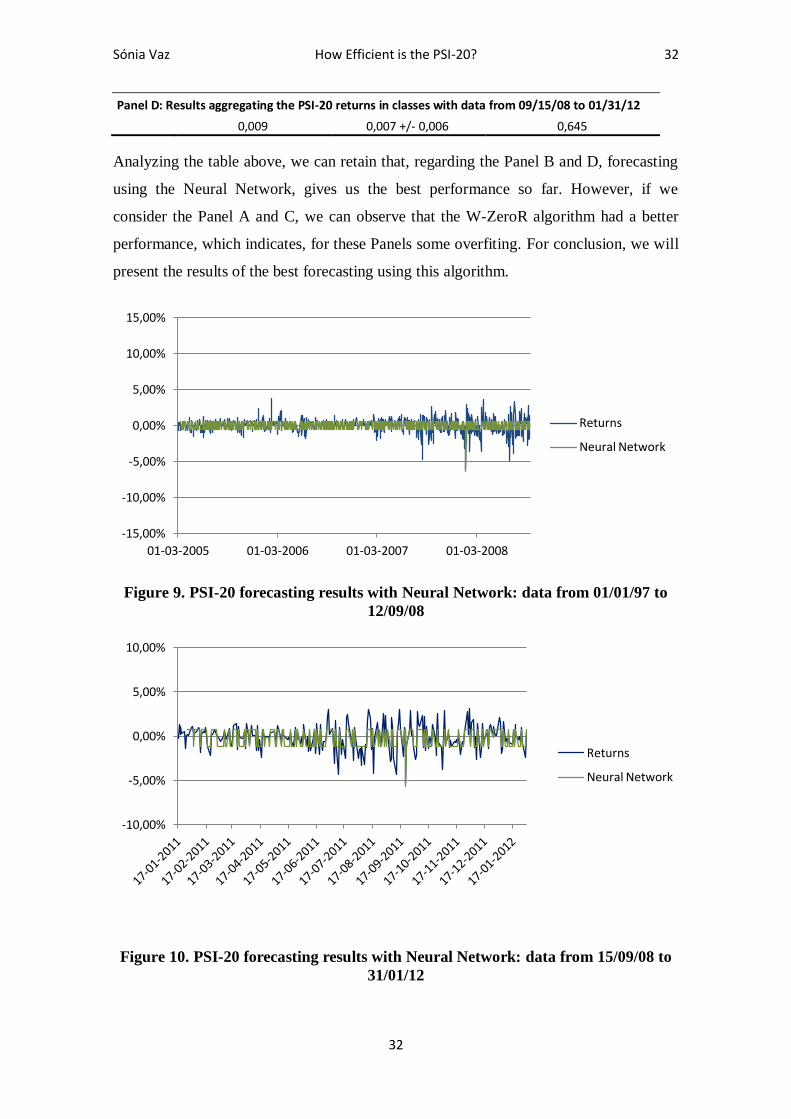
Sónia Vaz How Efficient is the PSI-20? 32
32
Panel D: Results aggregating the PSI-20 returns in classes with data from 09/15/08 to 01/31/12
0,009 0,007 +/- 0,006 0,645
Analyzing the table above, we can retain that, regarding the Panel B and D, forecasting
using the Neural Network, gives us the best performance so far. However, if we
consider the Panel A and C, we can observe that the W-ZeroR algorithm had a better
performance, which indicates, for these Panels some overfiting. For conclusion, we will
present the results of the best forecasting using this algorithm.
Figure 9. PSI-20 forecasting results with Neural Network: data from 01/01/97 to
12/09/08
Figure 10. PSI-20 forecasting results with Neural Network: data from 15/09/08 to
31/01/12
-15,00%
-10,00%
-5,00%
0,00%
5,00%
10,00%
15,00%
01-03-2005 01-03-2006 01-03-2007 01-03-2008
Returns
Neural Network
-10,00%
-5,00%
0,00%
5,00%
10,00%
Returns
Neural Network

Sónia Vaz How Efficient is the PSI-20? 33
33
5.2.4 Can we beat the market?
As earlier mentioned we will attempt to beat the market, using the best estimates of k-
NN and Neural Network.
Before we explain how we intend to do it, recalls that for the algorithms operate, our
initial data was split in order to 70% work as train and 30% as test. Being so, the data
we will now use concerns only those 30% which means that, the strategy is made with
respect to the data from 10/03/2005 to 12/09/2008, for the first period; and data from
26/01/2011 to 31/01/2012, for the second period.
In order to implement the strategy, first we defined the average of the returns predicted
either by k-NN either by Neural Network. Then, we calculated the moving average for 5
days and defined as a strategy to buy the index if the moving average was below the
average primarily calculated and to sell it if it was above. Finally we computed the
return we would obtain with this strategy and compare it with a buy and hold strategy.
The results were the ones presented at Table XI and assume as an assumption that there
are no transaction costs.
We also present in the Appendix A3 the histograms respecting the moving average for 5
days of the real PSI-20 returns, the k-NN prediction and the Neural Network prediction
concerning the first period of time (10/03/2005 to 12/09/2008); and in Appendix A4 the
same histograms but now with respect to the second period of time (26/01/2011 to
31/01/2012).
Table XI. Results of implementing the algorithms strategy
Real returns from a buy and hold strategy
Real returns from a strategy using k-NN predictions
Real returns from a strategy using Neural Network
predictions
Panel A: Data from 10/03/2005 to 12/09/2008
5,96% 39,18% 39,15%
Panel B: Data from 26/01/2011 to 31/12/2012
-37,28% -11,52% -11,52%
Looking at the Table XI, we can conclude that the real returns that we would obtain
using either the k-NN strategy either the Neural Network strategy are substantially
higher that the ones we would obtain using a buy and hold strategy.

Sónia Vaz How Efficient is the PSI-20? 34
34
6. Conclusions
In order to conclude this thesis is worth mentioning, regarding the Classical Efficiency
tests that all the indexes under analysis improve its efficiency after the subprime crisis,
with exception of the IBEX 35. It is also important to mention that, after the subprime
crisis, the DAX 30 did not reject the random walk hypothesis (or martingale process)
for any of the tests.
Based on the premise that if the market is efficient than it should not be possible to
forecast it, we introduced the algorithms as a complement of the classical tests for the
PSI-20 returns. This allows us to design a strategy based on the k-NN and on the Neural
Network predictions, and we conclude that would be possible to obtain significantly
higher earnings by the implementation of this strategy than using a simple buy-and-hold
strategy. Being so, this shows that the PSI-20 is not yet totally efficient, in fact as priory
confirmed by the classical tests.
In terms of other possible lines of research we believe it would be interesting to repeat
the tests mentioned in this dissertation, in a few years, to verify on the one hand if the
six European indexes chosen improve its efficiency, and on the other hand if it is
possible to obtain profits with the algorithms predictions. This will be useful because as
mentioned before, the techniques based on data mining will improve with time. Another
suggestion made is to consider transaction costs when designing the strategy “can we
beat the market?”.
Sónia Vaz How Efficient is the PSI-20? 35
35
Bibliography
Allen, H., & Taylor, M. (1992). The use of technical analysis in the foreign exchange
market. Journal of International Money and Finance 11 , 304-314.
Artus, P. (1995). Anomalies sur les marchés financiers. Ed. Economica.
Borges, M. R. (2008). Efficient Market Hypothesis in European Stock Markets. Lisbon:
ISEG, Working Paper 20/2008/DE/CIEF.
Borges, M. R. (2010). Efficient market hypothesis in European stock markets. The
European Journal of Finance , 16:7, 711-726.
Borges, M. R. (2011). Random walk tests for the Lisbon stock market. Applied
Economics , 43:5, 631-639.
Brooks, C. (2002). Introductory econometrics for finance. Cambridge: Cambridge
University Press.
Cabarkapa, S., Kojic, N., Savic, A., & Zivkovic, B. (2010). Use of artificial neural
networks in financial time series prediction and financial risk prediction. Infoteh-
Jahorina , 9, 584-587.
Chow, K., & Denning, K. (1993). A simple multiple variance ratio test. Journal of
Econometrics , 58, 385-401.
Dickey, D. A., & Fuller, W. A. (1979). Distribution of the Estimators for
Autoregressive Time Series With a Unit Root. Journal of the American Statistical
Association , 427-431.
Fama, E. (1970). Efficient Capital Markets: a Review of Theory and Empirical Work.
Journal of Finance 25 , 383-417.
Fama, E. (1991). Efficient Capital Markets: II. Journal of Finance, 46 , 1575-1617.
Ferson, W. E., Heuson, A., & Su, T. (2005). Weak-Form and Semi-Strong-Form Stock
Return Predictability Revisited. Management Science , 1582-1592.
Fuller, W. A. (1976). Introduction to Statistical Time Series. New York: Wiley.
Graham, B., & Dodd, D. L. (1934). Security analysis. NY: MacGraw-Hill.
Graham, B., & Dodd, D. L. (1934). Security Analysis. NY: McGraw-Hill.
Han, J., & Kamber, M. (2006). Data Minig Concepts and Techniques. San Francisco:
Elsevier.
Hill, T., O'Connor, M., & Remus, W. (1996). Neural Network Models for Time Series
Forecasts. Management Science , 1082-1092.
Sónia Vaz How Efficient is the PSI-20? 36
36
International Monetary Fund. (2011, April). World Economic Outlook. Retrieved June
1, 2012, from http://www.imf.org/external/pubs/ft/weo/2011/01/pdf/text.pdf
Isfan, M., Menezes, R., & Mendes, D. A. (2010). Forecasting the portuguese stock
market time series by using artificial neural networks. Journal of Physics: Conference
Series , 221, 1-13.
Jensen, M. C., & Benington, G. A. (1970). Random walks and technical theories: some
additional evidence. Journal of Finance , 469-481.
Kim, J. H. (2006). Wild bootstrapping variance ratio tests. Economics Letters , 92, 38-
43.
Koza, J. R. (1992). Genetic Programming: On the programming of computers by means
of natural selection. Cambridge: MIT Press.
LeRoy, S. F. (1989). Efficient Capital Markets and Martingales. Journal of Economic
Literature , 1583-1621.
Levy, R. A. (1968). Random Walk: Reality and Mith -- Reply. Financial Analysis
Journal , 129-132.
Levy, R. A. (1967). Random Walks: Reality or Myth. Financial Analysts Journal .
Lim, K.-P., Brooks, R. D., & Kim, J. H. (2008). Financial Crisis and Stock Market
Efficiency: Empirical Evidence from Asian Countries. International Review of
Financial Analysis , 571-591.
Lo, A., & MacKinlay, A. (1988). Stock market prices do not follow a random walk:
evidence from a simple specification test. The Review of Financial Studies , 1, 41-66.
Lo, A., & MacKinlay, A. (1989). The size and power of the variance ratio test in finite
samples. Journal of Econometrics , 40, 203-238.
McNelis, P. D. (2005). Neural Networks in finance: gaining predictive edge in the
market. Elsevier Academic Press.
Peña, D. (2005). Análisis de series temporales. Madrid: Alianza Editorial.
Quantitative Micro Software, LLC. (2009, November 29). Eviews 7 User's Guide II.
Retrieved May 31, 2012, from http://pt.scribd.com/doc/44246798/EViews-7-Users-
Guide-II
Samuelson, P. A. (1965). Proof that properly anticipated prices fluctuate randomly.
Industrial Management Review , 41-49.
Silva, N. M. (2001). Eficácia da Análise Técnica no Mercado Accionista Português.
Coimbra: Estudos do GEMF n. 9.
Sónia Vaz How Efficient is the PSI-20? 37
37
Smith, G., & Ryoo, H.-J. (2003). Variance Ratio Tests of the Random Walk Hypothesis
for European Emerging Stock Markets. The European Journal of Finance , 290-300.
Williams, J. B. (1938). The theory of investment value. Cambridge: Harvard U. Press.
Williams, J. B. (1938). The theory of investment value. Cambridge: Harvard U. Press.
Witten, I. H., Frank, E., Trigg, L., Hall, M., Holmes, G., & Cunningham, S. J. (1999).
Weka : Practical Machine Learning Tools and Techniques with Java Implementations.
(K. K, Ed.) Seminar, 99, 192-196. Retrieved April 20, 2012, from Citeseer:
http://citeseerx.ist.psu.edu/viewdoc/download?doi=10.1.1.157.9488&rep=rep1&type=p
df
Worthington, A., & Higgs, H. (2004). Random Walks and Market Efficiency in
European Equity Markets. Global Journal of Finance and Economics 1 , 59-78.
Wright, J. (2000). Alternative variance-ratio tests using ranks and signs. Journal of
Business and Economic Statistic , 18, 1-9.
Wu, X., Kumar, V., Quinlan, J. R., Ghosh, J., Yang, Q., Motoda, H., et al. (2008). Top
10 algorithms in data mining. Knowledge and Information Systems , 14 (1), 1-37.

Sónia Vaz How Efficient is the PSI-20? 38
38
Appendixes
A1. Histograms of the stock indexes’ returns from 01/01/1997 to 09/12/2012 and its
comparison with the Normal Distribution.
CAC 40 DAX 30
FTSE 100 FTSE ATHEX 20
IBEX 35 PSI 20
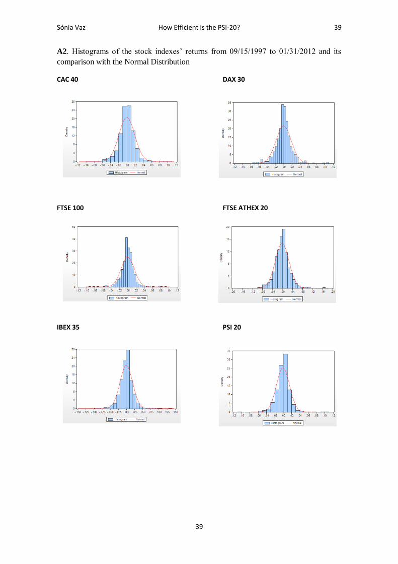
Sónia Vaz How Efficient is the PSI-20? 39
39
A2. Histograms of the stock indexes’ returns from 09/15/1997 to 01/31/2012 and its
comparison with the Normal Distribution
CAC 40 DAX 30
FTSE 100 FTSE ATHEX 20
IBEX 35 PSI 20
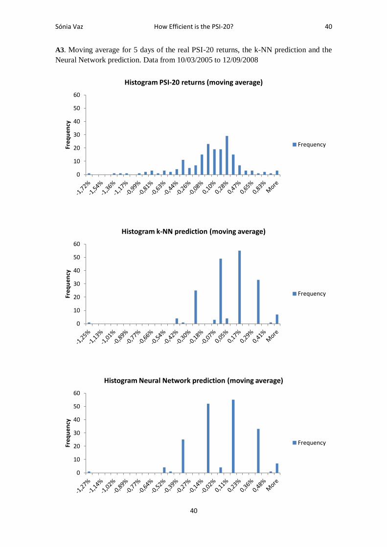
Sónia Vaz How Efficient is the PSI-20? 40
40
A3. Moving average for 5 days of the real PSI-20 returns, the k-NN prediction and the
Neural Network prediction. Data from 10/03/2005 to 12/09/2008
0
10
20
30
40
50
60
Fre
qu
en
cy
Histogram PSI-20 returns (moving average)
Frequency
0
10
20
30
40
50
60
Fre
qu
ency
Histogram k-NN prediction (moving average)
Frequency
0
10
20
30
40
50
60
Fre
qu
ency
Histogram Neural Network prediction (moving average)
Frequency
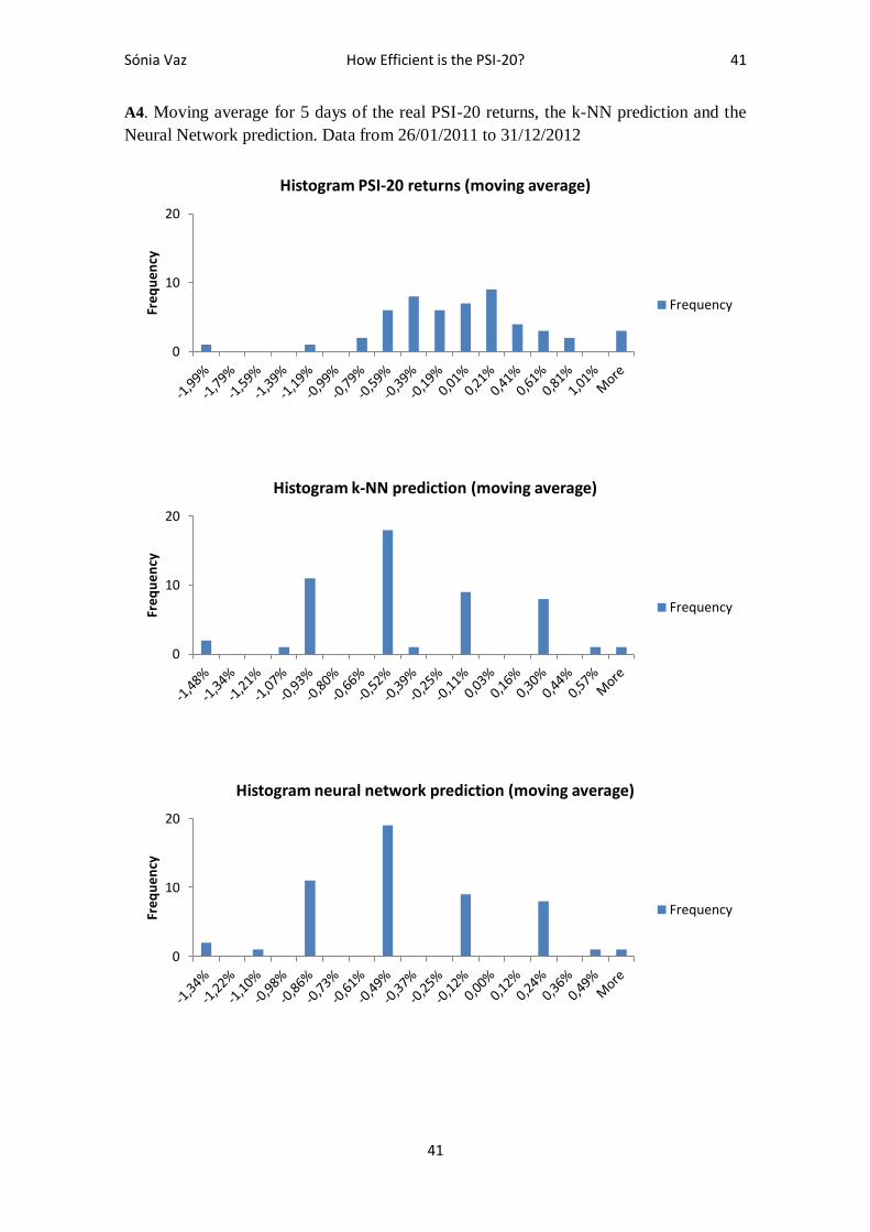
Sónia Vaz How Efficient is the PSI-20? 41
41
A4. Moving average for 5 days of the real PSI-20 returns, the k-NN prediction and the
Neural Network prediction. Data from 26/01/2011 to 31/12/2012
0
10
20
Fre
qu
en
cy
Histogram PSI-20 returns (moving average)
Frequency
0
10
20
Fre
qu
en
cy
Histogram k-NN prediction (moving average)
Frequency
0
10
20
Fre
qu
ency
Histogram neural network prediction (moving average)
Frequency