MapReduce: Parallel Programming in the Cloud - … · MapReduce: Parallel Programming in the Cloud Brad Karp ... file to final output file after writes finish; ... • Partitioning

MapReduce:Parallel Programming in the Cloud

Brad KarpUCL Computer Science

(with slides contributed by Kyle Jamieson)

CS M038 / GZ064th March 2016

Motivation

• By 2004, many web data sets were very large (10s−100s of terabytes)– Could not analyze them on a single server– Too much data, computation; using a

supercomputer would be expensive

• Standard architecture has emerged– Cluster of commodity machines– Gigabit Ethernet interconnect, racks arranged in tree

topology

• How to organize computation on this architecture?– Mask issues such as hardware failure

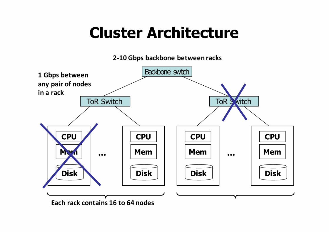
Cluster Architecture

Mem

Disk

CPU

Mem

Disk

CPU

…

ToR Switch

Eachrackcontains16to64nodes

Mem

Disk

CPU

Mem

Disk

CPU

…

ToR Switch

Backbone switch1Gbpsbetweenanypairofnodesinarack

2-10Gbpsbackbonebetweenracks

Stable Storage• First-order problem: if nodes can fail, how can we store

data persistently?

• Answer: A replicated, distributed file system– Provides a global file namespace abstraction

– Provides a unified view of the file system and hides the details of replication and consistency management

– Examples: Google’s GFS, Hadoop File System (HDFS)

• Typical usage pattern– Huge files (100s of GB to TB)– Data is rarely updated in place– Reads and appends are common

GFS Distributed File System

• Each file is split into contiguous 64 Mbyte chunks

• GFS cluster is made up of two types of nodes:1. Large number of Chunkservers

• Each chunk replicated, usually 3× (GFS)• Try to keep replicas in chunkservers in different racks (why?)

2. One Master node• Stores metadata; might be replicated

• Link GFS client library into applications– Talks to master to find chunk servers – Then connects directly to chunkservers to access data

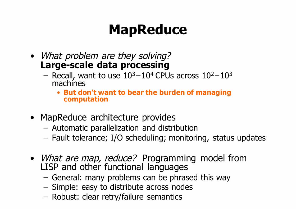
MapReduce• What problem are they solving?

Large-scale data processing– Recall, want to use 103−104 CPUs across 102−103

machines• But don’t want to bear the burden of managing

computation

• MapReduce architecture provides– Automatic parallelization and distribution– Fault tolerance; I/O scheduling; monitoring, status updates

• What are map, reduce? Programming model from LISP and other functional languages– General: many problems can be phrased this way– Simple: easy to distribute across nodes– Robust: clear retry/failure semantics

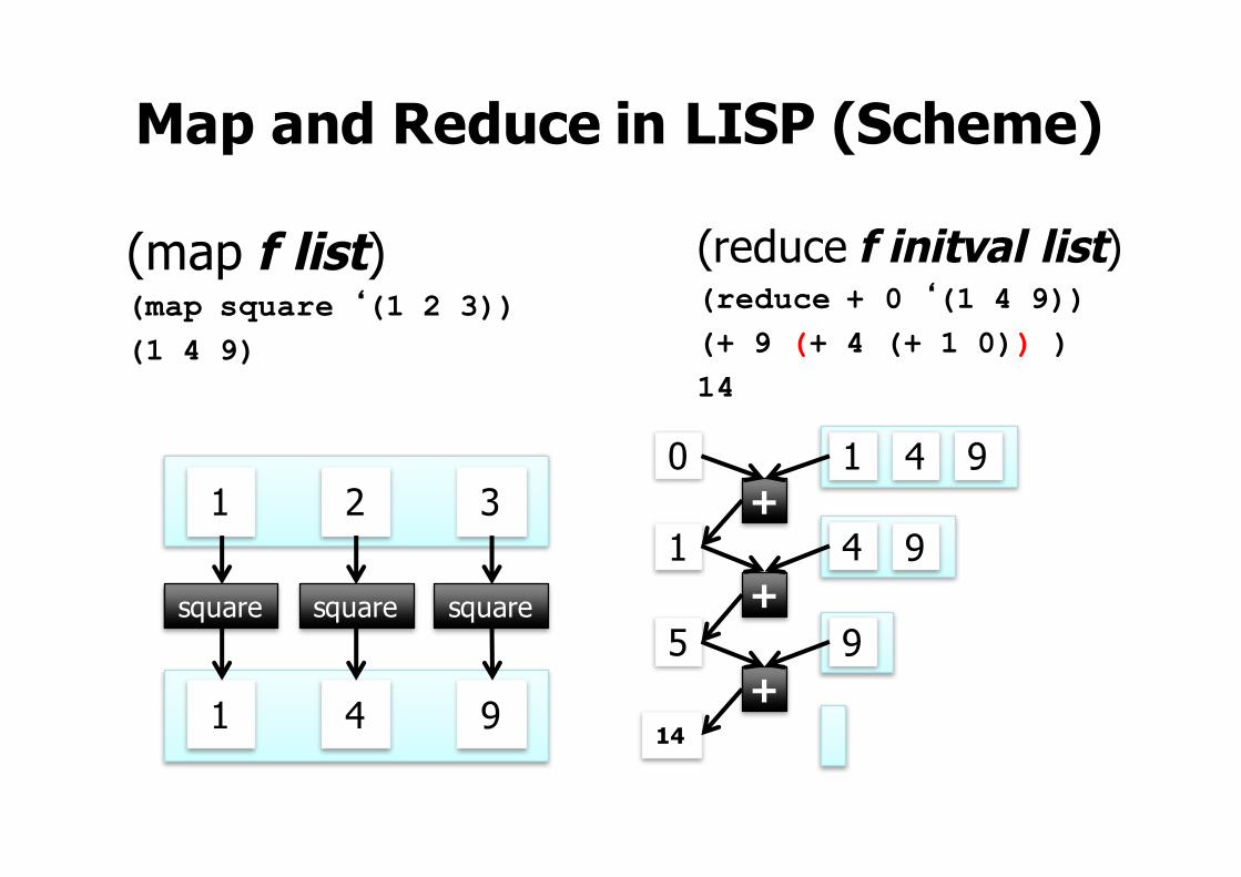
Map and Reduce in LISP (Scheme)

(map f list)(map square ‘(1 2 3)) (1 4 9)

(reduce f initval list)(reduce + 0 ‘(1 4 9))(+ 9 (+ 4 (+ 1 0)) )14

1 2 3

square square square

1 4 9

1 4 90+

1 4 9

9+

5

14+

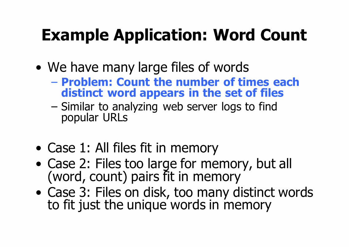
Example Application: Word Count

• We have many large files of words– Problem: Count the number of times each

distinct word appears in the set of files– Similar to analyzing web server logs to find

popular URLs

• Case 1: All files fit in memory• Case 2: Files too large for memory, but all

(word, count) pairs fit in memory• Case 3: Files on disk, too many distinct words

to fit just the unique words in memory

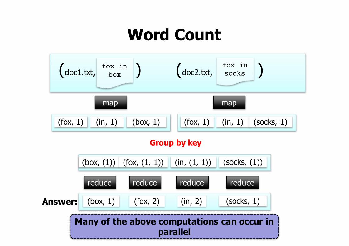
Word Countfox in socks

fox in box(doc1.txt, ) (doc2.txt, )

(fox, 1) (in, 1) (box, 1) (fox, 1) (in, 1) (socks, 1)

map map

(in, (1, 1))(box, (1)) (fox, (1, 1)) (socks, (1))

reduce reduce reduce reduce

(in, 2)(box, 1) (fox, 2) (socks, 1)

Many of the above computations can occur in parallel

Answer:

Group by key

MapReduce

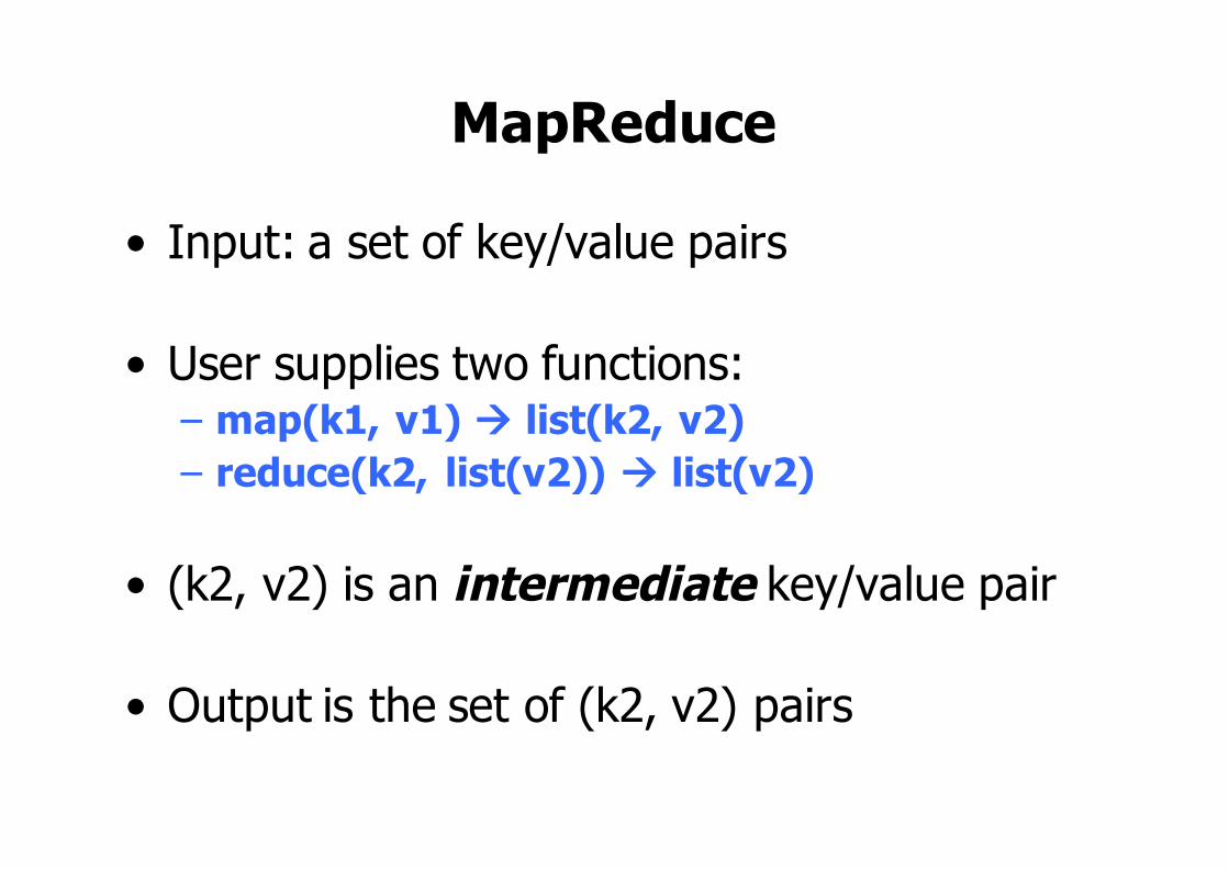
• Input: a set of key/value pairs

• User supplies two functions:– map(k1, v1) à list(k2, v2)– reduce(k2, list(v2)) à list(v2)

• (k2, v2) is an intermediate key/value pair

• Output is the set of (k2, v2) pairs

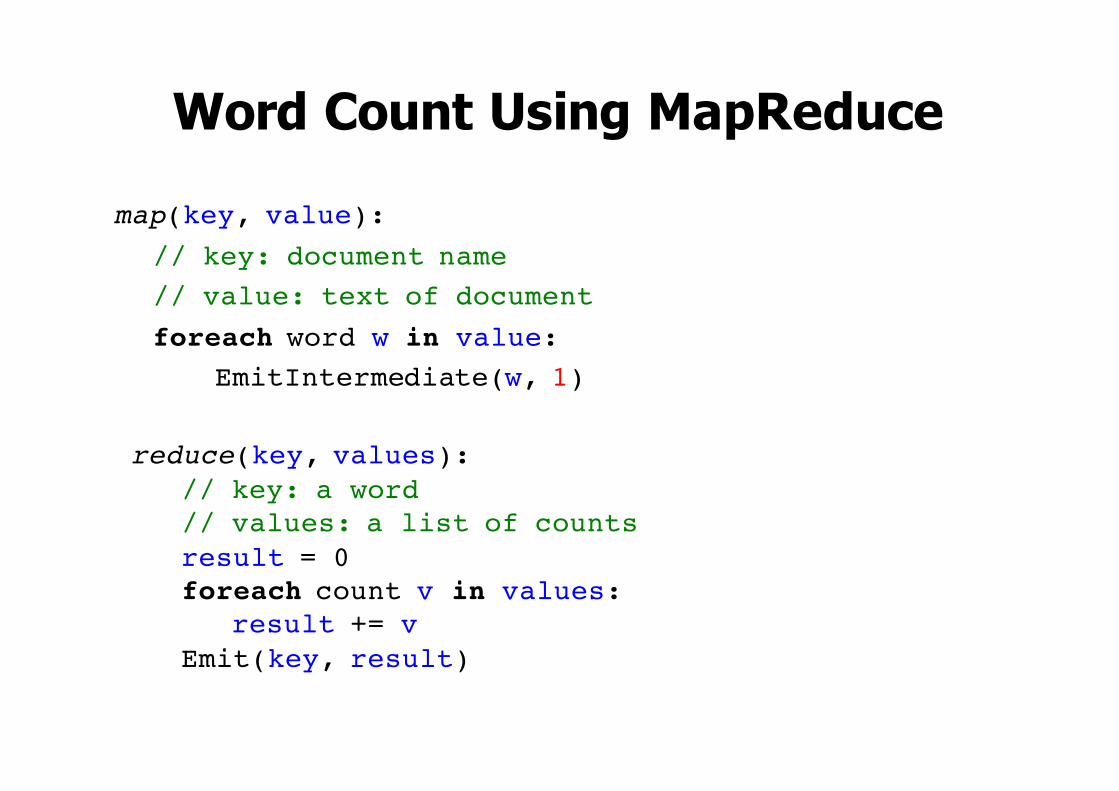
Word Count Using MapReducemap(key, value):

// key: document name// value: text of documentforeach word w in value:

EmitIntermediate(w, 1)

reduce(key, values):// key: a word// values: a list of countsresult = 0foreach count v in values:

result += vEmit(key, result)

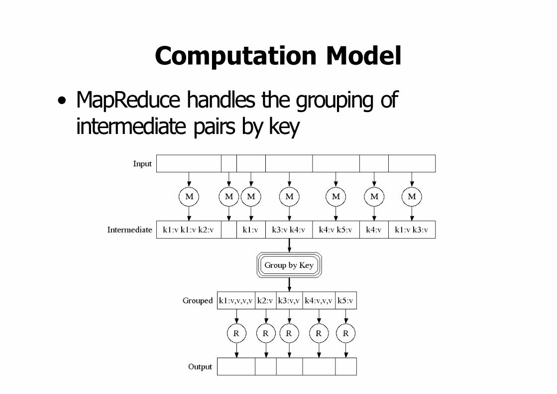
Computation Model• MapReduce handles the grouping of

intermediate pairs by key

Implementation Overview

• Typical cluster: 100s of 2-CPU machines, 4−8 GB RAM

– Limited bisection bandwidth: divide network into any two parts; take minimum bandwidth between parts

– GFS manages input and output data

• MapReduce Job scheduling system: jobs made up of tasks, scheduler assigns tasks to machines

• Implementation is a C++ library linked into user programs

MapReduce Execution Overview

UserProgram

Master

(1) fork

worker

(1) fork

worker

(1) fork

(2)assignmap

(2)assignreduce

split 0

split 1

split 2

split 3

split 4

outputfile 0

(6) write

worker(3) read

worker

(4) local write

Mapphase

Intermediate files(on local disks)

worker outputfile 1

Inputfiles

(5) remote read

Reducephase

Outputfiles

Figure 1: Execution overview

Inverted Index: The map function parses each docu-ment, and emits a sequence of ⟨word,document ID⟩pairs. The reduce function accepts all pairs for a givenword, sorts the corresponding document IDs and emits a⟨word, list(document ID)⟩ pair. The set of all outputpairs forms a simple inverted index. It is easy to augmentthis computation to keep track of word positions.

Distributed Sort: The map function extracts the keyfrom each record, and emits a ⟨key,record⟩ pair. Thereduce function emits all pairs unchanged. This compu-tation depends on the partitioning facilities described inSection 4.1 and the ordering properties described in Sec-tion 4.2.

3 Implementation

Many different implementations of the MapReduce in-terface are possible. The right choice depends on theenvironment. For example, one implementation may besuitable for a small shared-memory machine, another fora large NUMA multi-processor, and yet another for aneven larger collection of networked machines.This section describes an implementation targetedto the computing environment in wide use at Google:

large clusters of commodity PCs connected together withswitched Ethernet [4]. In our environment:

(1)Machines are typically dual-processor x86 processorsrunning Linux, with 2-4 GB of memory per machine.

(2) Commodity networking hardware is used – typicallyeither 100 megabits/second or 1 gigabit/second at themachine level, but averaging considerably less in over-all bisection bandwidth.

(3) A cluster consists of hundreds or thousands of ma-chines, and therefore machine failures are common.

(4) Storage is provided by inexpensive IDE disks at-tached directly to individual machines. A distributed filesystem [8] developed in-house is used to manage the datastored on these disks. The file system uses replication toprovide availability and reliability on top of unreliablehardware.

(5) Users submit jobs to a scheduling system. Each jobconsists of a set of tasks, and is mapped by the schedulerto a set of available machines within a cluster.

3.1 Execution Overview

The Map invocations are distributed across multiplemachines by automatically partitioning the input data

To appear in OSDI 2004 3

M

(in GFS) (R files in GFS)

R = 2

R

R

(R = 2 workers)

How Many Map and Reduce Jobs?

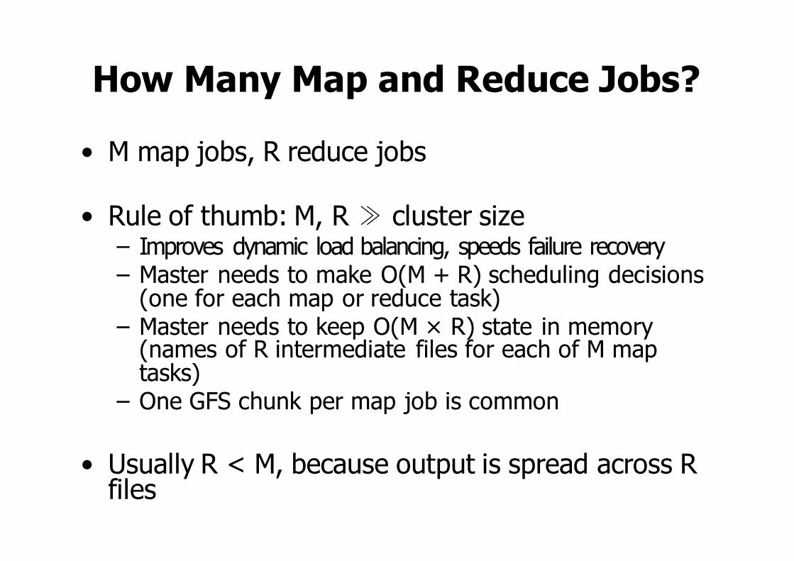
• M map jobs, R reduce jobs

• Rule of thumb: M, R ≫ cluster size– Improves dynamic load balancing, speeds failure recovery – Master needs to make O(M + R) scheduling decisions

(one for each map or reduce task)– Master needs to keep O(M × R) state in memory

(names of R intermediate files for each of M map tasks)

– One GFS chunk per map job is common

• Usually R < M, because output is spread across R files

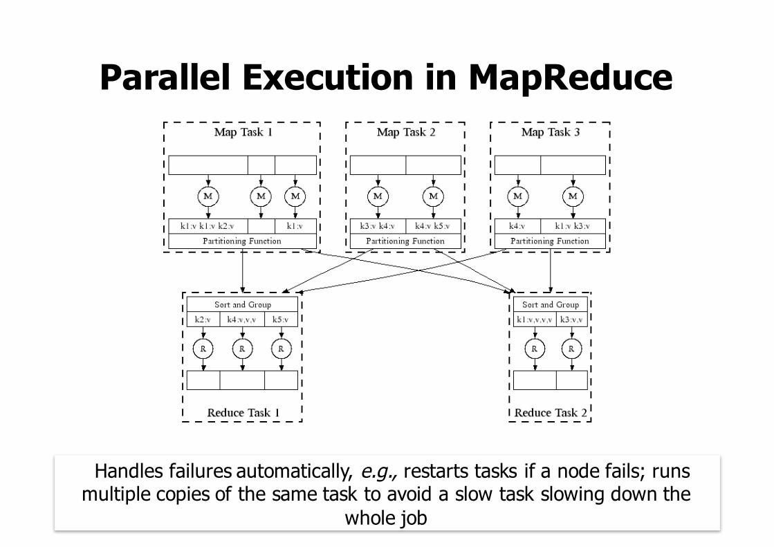
Parallel Execution in MapReduce

Handles failures automatically, e.g., restarts tasks if a node fails; runs multiple copies of the same task to avoid a slow task slowing down the

whole job

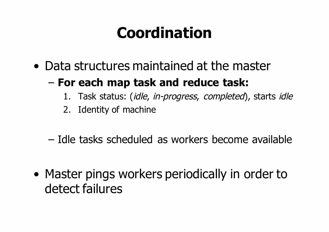
Coordination

• Data structures maintained at the master– For each map task and reduce task:

1. Task status: (idle, in-progress, completed), starts idle2. Identity of machine

– Idle tasks scheduled as workers become available

• Master pings workers periodically in order to detect failures

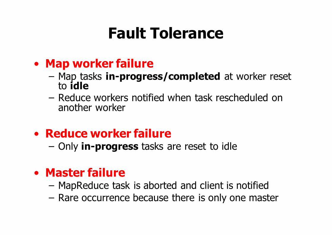
Fault Tolerance

• Map worker failure– Map tasks in-progress/completed at worker reset

to idle– Reduce workers notified when task rescheduled on

another worker

• Reduce worker failure– Only in-progress tasks are reset to idle

• Master failure– MapReduce task is aborted and client is notified– Rare occurrence because there is only one master

Semantics in the Presence of Failures

• Claim: Distributed MapReduce implementation produces same output as a non-faulting local execution (with deterministic operators)

• Atomic commits of map/reduce tasks: Either it all happens exactly once, or no effects are observable.– Map tasks: worker sends completion message to

master with names of R temporary files after writes finish; master accepts only one.

– Reduce task: Atomic rename of temporary output file to final output file after writes finish; file system guarantees just one execution.

Combiners

• Often a map task will produce many pairs of the form (k, v1), (k, v2), … for the same key k– e.g., popular words in word count example

• Can save network time by “pre-aggregating” at map worker– combine(k1, list(v1)) à v2– Usually same as reduce function

• Works only if reduce function is commutative and associative

Partitioning Function• Inputs to map tasks are created by contiguous

splits of input file

• For reduce, we need to ensure that records with the same intermediate key end up at the same worker

• System uses a default partition function e.g., hash(key) mod R

• Sometimes useful to override:– e.g., suppose we are counting URL access

frequencies• Partitioning function hash(hostname(URL)) mod R

ensures all URLs from a given host end up in the same output file

Performance: Stragglers

• Machine that takes unusually long time to complete one of the last few map or reduce tasks in a computation

• Why does this happen?– Bad disk: errors slow down– CPU load high– Configuration bug disables CPU cache

• Fix: When close to completion, master schedules backup tasks: executions of remaining in-progress tasks– Task completes when either primary or backup

completes– Atomicity properties above guarantee correctness.

Data Transfer Rates for sort Program

500 10000

5000

10000

15000

20000

Inpu

t (M

B/s)

500 10000

5000

10000

15000

20000

Shuf

fle (M

B/s)

500 1000Seconds

0

5000

10000

15000

20000

Out

put (

MB/

s)

Done

(a) Normal execution

500 10000

5000

10000

15000

20000

Inpu

t (M

B/s)

500 10000

5000

10000

15000

20000

Shuf

fle (M

B/s)

500 1000Seconds

0

5000

10000

15000

20000

Out

put (

MB/

s)

Done

(b) No backup tasks

500 10000

5000

10000

15000

20000

Inpu

t (M

B/s)

500 10000

5000

10000

15000

20000

Shuf

fle (M

B/s)

500 1000Seconds

0

5000

10000

15000

20000

Out

put (

MB/

s)

Done

(c) 200 tasks killed

Figure 3: Data transfer rates over time for different executions of the sort program

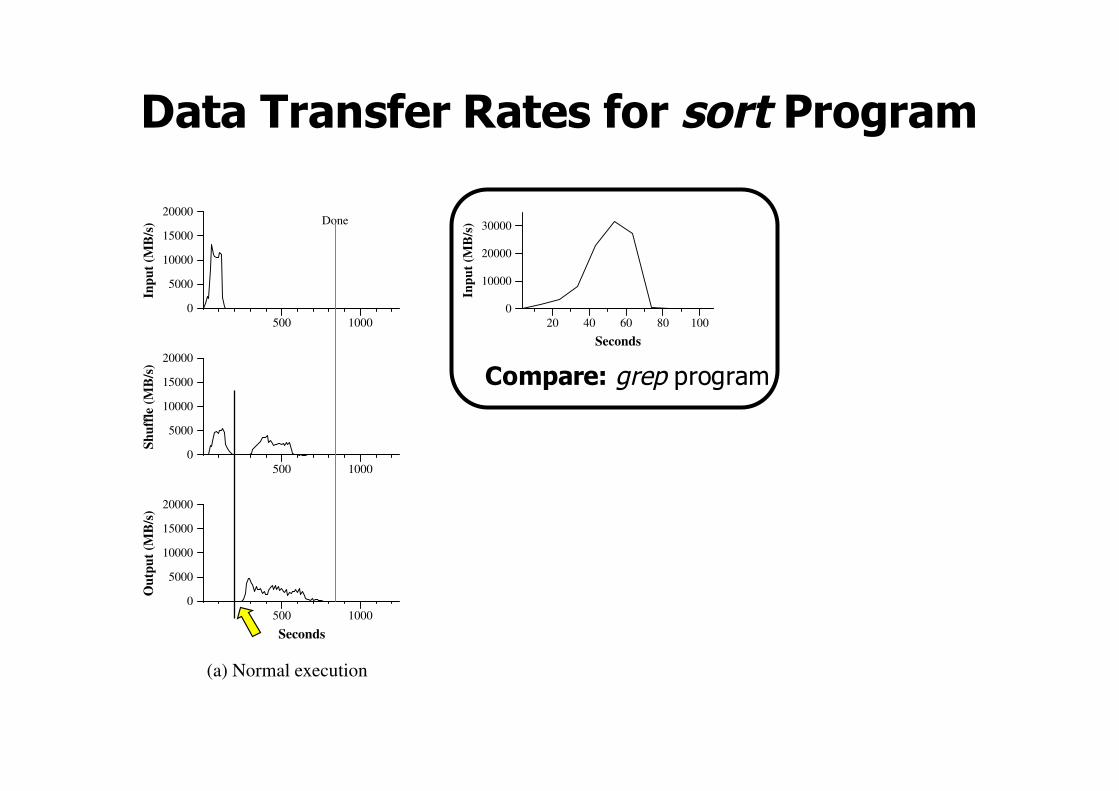
original text line as the intermediate key/value pair. Weused a built-in Identity function as the Reduce operator.This functions passes the intermediate key/value pair un-changed as the output key/value pair. The final sortedoutput is written to a set of 2-way replicated GFS files(i.e., 2 terabytes are written as the output of the program).As before, the input data is split into 64MB pieces(M = 15000). We partition the sorted output into 4000files (R = 4000). The partitioning function uses the ini-tial bytes of the key to segregate it into one of R pieces.Our partitioning function for this benchmark has built-in knowledge of the distribution of keys. In a generalsorting program, we would add a pre-pass MapReduceoperation that would collect a sample of the keys anduse the distribution of the sampled keys to compute split-points for the final sorting pass.Figure 3 (a) shows the progress of a normal executionof the sort program. The top-left graph shows the rateat which input is read. The rate peaks at about 13 GB/sand dies off fairly quickly since all map tasks finish be-fore 200 seconds have elapsed. Note that the input rateis less than for grep. This is because the sort map tasksspend about half their time and I/O bandwidth writing in-termediate output to their local disks. The correspondingintermediate output for grep had negligible size.The middle-left graph shows the rate at which datais sent over the network from the map tasks to the re-duce tasks. This shuffling starts as soon as the firstmap task completes. The first hump in the graph is for

the first batch of approximately 1700 reduce tasks (theentire MapReduce was assigned about 1700 machines,and each machine executes at most one reduce task at atime). Roughly 300 seconds into the computation, someof these first batch of reduce tasks finish and we startshuffling data for the remaining reduce tasks. All of theshuffling is done about 600 seconds into the computation.The bottom-left graph shows the rate at which sorteddata is written to the final output files by the reduce tasks.There is a delay between the end of the first shuffling pe-riod and the start of the writing period because the ma-chines are busy sorting the intermediate data. The writescontinue at a rate of about 2-4 GB/s for a while. All ofthe writes finish about 850 seconds into the computation.Including startup overhead, the entire computation takes891 seconds. This is similar to the current best reportedresult of 1057 seconds for the TeraSort benchmark [18].A few things to note: the input rate is higher than theshuffle rate and the output rate because of our localityoptimization – most data is read from a local disk andbypasses our relatively bandwidth constrained network.The shuffle rate is higher than the output rate becausethe output phase writes two copies of the sorted data (wemake two replicas of the output for reliability and avail-ability reasons). We write two replicas because that isthe mechanism for reliability and availability providedby our underlying file system. Network bandwidth re-quirements for writing data would be reduced if the un-derlying file system used erasure coding [14] rather thanreplication.


Counter* uppercase;uppercase = GetCounter("uppercase");

map(String name, String contents):for each word w in contents:if (IsCapitalized(w)):uppercase->Increment();

EmitIntermediate(w, "1");

The counter values from individual worker machinesare periodically propagated to the master (piggybackedon the ping response). The master aggregates the countervalues from successful map and reduce tasks and returnsthem to the user code when the MapReduce operationis completed. The current counter values are also dis-played on the master status page so that a human canwatch the progress of the live computation. When aggre-gating counter values, the master eliminates the effects ofduplicate executions of the same map or reduce task toavoid double counting. (Duplicate executions can arisefrom our use of backup tasks and from re-execution oftasks due to failures.)Some counter values are automatically maintainedby the MapReduce library, such as the number of in-put key/value pairs processed and the number of outputkey/value pairs produced.Users have found the counter facility useful for san-ity checking the behavior of MapReduce operations. Forexample, in some MapReduce operations, the user codemay want to ensure that the number of output pairsproduced exactly equals the number of input pairs pro-cessed, or that the fraction of German documents pro-cessed is within some tolerable fraction of the total num-ber of documents processed.

5 Performance

In this section we measure the performance of MapRe-duce on two computations running on a large cluster ofmachines. One computation searches through approxi-mately one terabyte of data looking for a particular pat-tern. The other computation sorts approximately one ter-abyte of data.These two programs are representative of a large sub-set of the real programswritten by users of MapReduce –one class of programs shuffles data from one representa-tion to another, and another class extracts a small amountof interesting data from a large data set.

5.1 Cluster ConfigurationAll of the programs were executed on a cluster thatconsisted of approximately 1800 machines. Each ma-chine had two 2GHz Intel Xeon processors with Hyper-Threading enabled, 4GB of memory, two 160GB IDE

20 40 60 80 100Seconds

0

10000

20000

30000

Inpu

t (M

B/s)

Figure 2: Data transfer rate over time

disks, and a gigabit Ethernet link. The machines werearranged in a two-level tree-shaped switched networkwith approximately 100-200 Gbps of aggregate band-width available at the root. All of the machines werein the same hosting facility and therefore the round-triptime between any pair of machines was less than a mil-lisecond.Out of the 4GB of memory, approximately 1-1.5GBwas reserved by other tasks running on the cluster. Theprograms were executed on a weekend afternoon, whenthe CPUs, disks, and network were mostly idle.

5.2 Grep

The grep program scans through 1010 100-byte records,searching for a relatively rare three-character pattern (thepattern occurs in 92,337 records). The input is split intoapproximately 64MB pieces (M = 15000), and the en-tire output is placed in one file (R = 1).Figure 2 shows the progress of the computation overtime. The Y-axis shows the rate at which the input data isscanned. The rate gradually picks up as more machinesare assigned to this MapReduce computation, and peaksat over 30 GB/s when 1764 workers have been assigned.As the map tasks finish, the rate starts dropping and hitszero about 80 seconds into the computation. The entirecomputation takes approximately 150 seconds from startto finish. This includes about a minute of startup over-head. The overhead is due to the propagation of the pro-gram to all worker machines, and delays interacting withGFS to open the set of 1000 input files and to get theinformation needed for the locality optimization.

5.3 Sort

The sort program sorts 1010 100-byte records (approxi-mately 1 terabyte of data). This program is modeled afterthe TeraSort benchmark [10].The sorting program consists of less than 50 lines ofuser code. A three-line Map function extracts a 10-bytesorting key from a text line and emits the key and the


Compare: grep program

Disabling Backup Tasks Lets Stragglers Delay Job Finish Time

500 10000

5000

10000

15000

20000

Inpu

t (M

B/s)

500 10000

5000

10000

15000

20000

Shuf

fle (M

B/s)

500 1000Seconds

0

5000

10000

15000

20000

Out

put (

MB/

s)

Done


500 10000

5000

10000

15000

20000

Inpu

t (M

B/s)

500 10000

5000

10000

15000

20000

Shuf

fle (M

B/s)

500 1000Seconds

0

5000

10000

15000

20000

Out

put (

MB/

s)

Done

(b) No backup tasks

500 10000

5000

10000

15000

20000

Inpu

t (M

B/s)

500 10000

5000

10000

15000

20000

Shuf

fle (M

B/s)

500 1000Seconds

0

5000

10000

15000

20000

Out

put (

MB/

s)

Done






Effect of Machine Failures

500 10000

5000

10000

15000

20000

Inpu

t (M

B/s)

500 10000

5000

10000

15000

20000

Shuf

fle (M

B/s)

500 1000Seconds

0

5000

10000

15000

20000

Out

put (

MB/

s)

Done


500 10000

5000

10000

15000

20000

Inpu

t (M

B/s)

500 10000

5000

10000

15000

20000

Shuf

fle (M

B/s)

500 1000Seconds

0

5000

10000

15000

20000

Out

put (

MB/

s)

Done

(b) No backup tasks

500 10000

5000

10000

15000

20000

Inpu

t (M

B/s)

500 10000

5000

10000

15000

20000

Shuf

fle (M

B/s)

500 1000Seconds

0

5000

10000

15000

20000

Out

put (

MB/

s)

Done






2003−2004: MapReduce Catches On

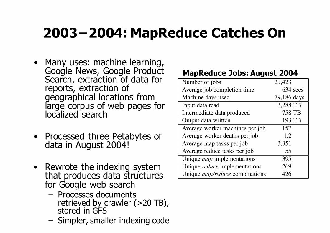
• Many uses: machine learning, Google News, Google Product Search, extraction of data for reports, extraction of geographical locations from large corpus of web pages for localized search

• Processed three Petabytes of data in August 2004!

• Rewrote the indexing system that produces data structures for Google web search– Processes documents

retrieved by crawler (>20 TB), stored in GFS

– Simpler, smaller indexing code

5.4 Effect of Backup Tasks

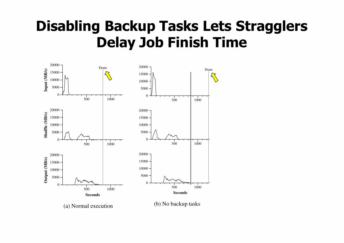
In Figure 3 (b), we show an execution of the sort pro-gram with backup tasks disabled. The execution flow issimilar to that shown in Figure 3 (a), except that there isa very long tail where hardly any write activity occurs.After 960 seconds, all except 5 of the reduce tasks arecompleted. However these last few stragglers don’t fin-ish until 300 seconds later. The entire computation takes1283 seconds, an increase of 44% in elapsed time.

5.5 Machine Failures

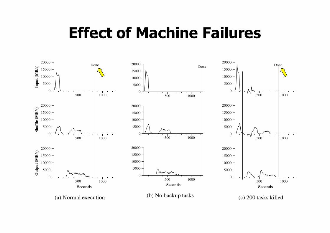
In Figure 3 (c), we show an execution of the sort programwhere we intentionally killed 200 out of 1746 workerprocesses several minutes into the computation. Theunderlying cluster scheduler immediately restarted newworker processes on these machines (since only the pro-cesses were killed, the machines were still functioningproperly).The worker deaths show up as a negative input ratesince some previously completed map work disappears(since the corresponding map workers were killed) andneeds to be redone. The re-execution of this map workhappens relatively quickly. The entire computation fin-ishes in 933 seconds including startup overhead (just anincrease of 5% over the normal execution time).

6 Experience

We wrote the first version of the MapReduce library inFebruary of 2003, and made significant enhancements toit in August of 2003, including the locality optimization,dynamic load balancing of task execution across workermachines, etc. Since that time, we have been pleasantlysurprised at how broadly applicable the MapReduce li-brary has been for the kinds of problems we work on.It has been used across a wide range of domains withinGoogle, including:

• large-scale machine learning problems,

• clustering problems for the Google News andFroogle products,

• extraction of data used to produce reports of popularqueries (e.g. Google Zeitgeist),

• extraction of properties of web pages for new exper-iments and products (e.g. extraction of geographi-cal locations from a large corpus of web pages forlocalized search), and

• large-scale graph computations.

2003/03

2003/06

2003/09

2003/12

2004/03

2004/06

2004/090

200

400

600

800

1000

Num

ber

of in

stan

ces i

n so

urce

tree

Figure 4: MapReduce instances over time

Number of jobs 29,423Average job completion time 634 secsMachine days used 79,186 daysInput data read 3,288 TBIntermediate data produced 758 TBOutput data written 193 TBAverage worker machines per job 157Average worker deaths per job 1.2Average map tasks per job 3,351Average reduce tasks per job 55Unique map implementations 395Unique reduce implementations 269Unique map/reduce combinations 426

Table 1: MapReduce jobs run in August 2004

Figure 4 shows the significant growth in the number ofseparate MapReduce programs checked into our primarysource code management system over time, from 0 inearly 2003 to almost 900 separate instances as of lateSeptember 2004. MapReduce has been so successful be-cause it makes it possible to write a simple program andrun it efficiently on a thousand machines in the courseof half an hour, greatly speeding up the development andprototyping cycle. Furthermore, it allows programmerswho have no experience with distributed and/or parallelsystems to exploit large amounts of resources easily.At the end of each job, the MapReduce library logsstatistics about the computational resources used by thejob. In Table 1, we show some statistics for a subset ofMapReduce jobs run at Google in August 2004.

6.1 Large-Scale Indexing

One of our most significant uses of MapReduce to datehas been a complete rewrite of the production index-


MapReduce Jobs: August 2004

Use Case: PageRank,Random Walks on the Web

• How can we measure how popular a web page is?

• If a user starts at a random web page and surfs by clicking links and randomly entering new URLs, what is the probability that s/he will arrive at a given page?

• The PageRank of a page captures this notion– More “popular” or “worthwhile” pages get a

higher rank

PageRank: Visually

www.cnn.com

en.wikipedia.org

www.nytimes.com

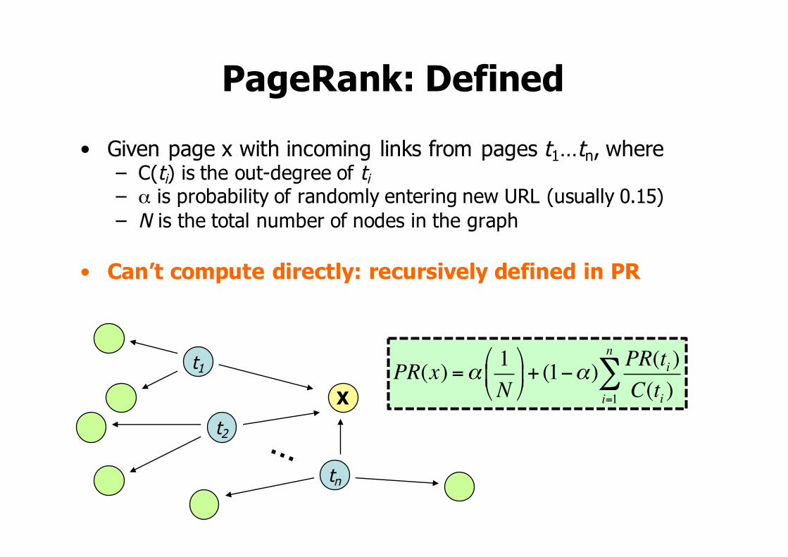
PageRank: Defined• Given page x with incoming links from pages t1…tn, where

– C(ti) is the out-degree of ti– α is probability of randomly entering new URL (usually 0.15)– N is the total number of nodes in the graph

• Can’t compute directly: recursively defined in PR

PR(x) =α 1N!

"#

$

%&+ (1−α)

PR(ti )C(ti )i=1

n

∑X

t1

t2

tn

PageRank Computation: Intuition

• Calculation is iterative: maintain an estimate of PageRank at iteration i: PRi

• Sketch of algorithm– Start with seed PRi values– PRi+1 is based on PRi: each page distributes PRi “credit” to

all pages it links to– Each target page adds up “credit” from inbound links to

compute PRi+1– Iterate until values converge

• Each page distributes its PRi to all pages it links to. Link targets add up their awarded rank fragments to find their PRi+1

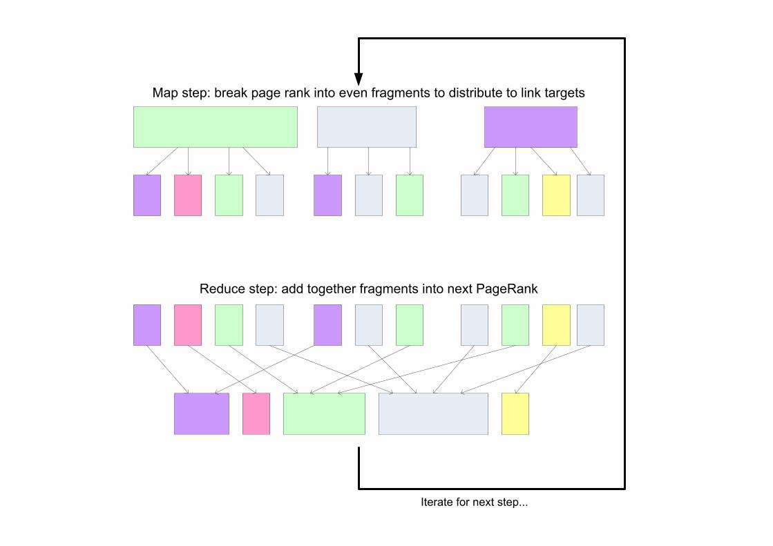
Map step: break page rank into even fragments to distribute to link targets

Reduce step: add together fragments into next PageRank

Iterate for next step...

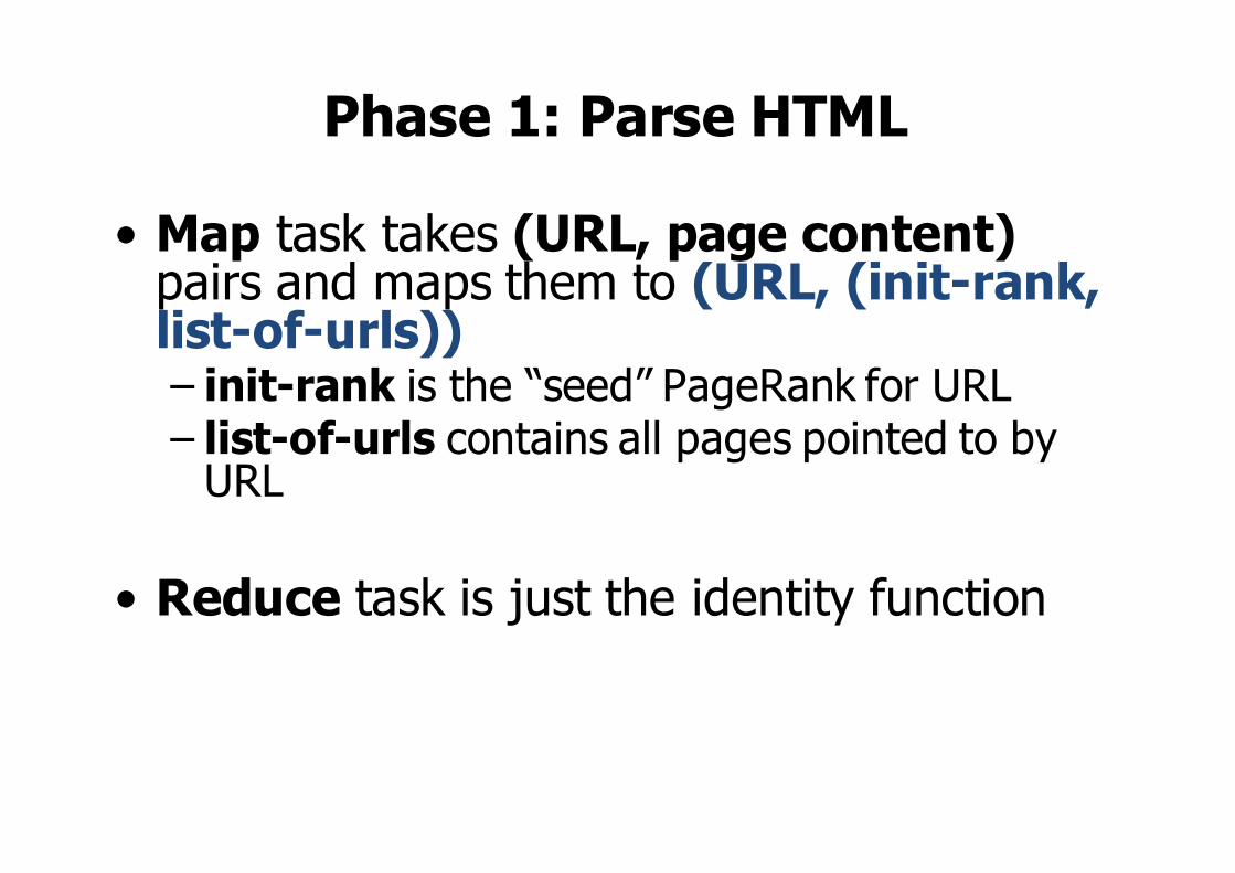
Phase 1: Parse HTML

• Map task takes (URL, page content) pairs and maps them to (URL, (init-rank, list-of-urls))– init-rank is the “seed” PageRank for URL– list-of-urls contains all pages pointed to by

URL

• Reduce task is just the identity function

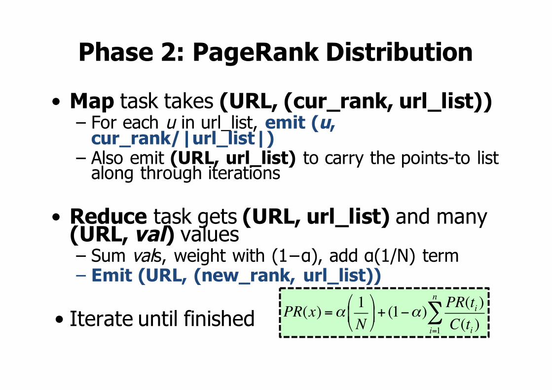
Phase 2: PageRank Distribution

• Map task takes (URL, (cur_rank, url_list))– For each u in url_list, emit (u,

cur_rank/|url_list|)– Also emit (URL, url_list) to carry the points-to list

along through iterations

• Reduce task gets (URL, url_list) and many (URL, val) values– Sum vals, weight with (1−α), add α(1/N) term– Emit (URL, (new_rank, url_list))

• Iterate until finished PR(x) =α 1N!

"#

$

%&+ (1−α)

PR(ti )C(ti )i=1

n

∑

PageRank Use Case Lessons

• MapReduce runs the “heavy lifting” in iterated computation

• Key element in parallelization is independent PageRank computations in a given step

• Parallelization requires thinking about minimum data partitions to transmit (e.g., compact representations of graph rows)– Even the implementation shown today doesn't

actually scale to the whole web, but it works for intermediate-sized graphs

Follow-on Reading(non-examinable)

Percolator, Peng and Dabek (USENIX OSDI ’10)

• System for incrementally processing updates to a large data set

• Deployed to create the Google web search index

• Replaces batch-based indexing with incremental processing

• Reduces the average age of documents in Google search results by 50%

Administrivia

• Student presentation slots posted to M038/GZ06 class calendar page

• Regardless of presentation slot, must submit final slides by start of lecture (10:05 AM) on 11th March (this Friday)– No changes allowed after submission

• One one-pager assigned per lecture on student presentation days 36

Documents

MapReduce: Parallel Programming in the Cloud - … · MapReduce: Parallel Programming in the Cloud Brad Karp ... file to final output file after writes finish; ... • Partitioning