Embed Size (px)
Citation preview

This article was downloaded by: [University of Haifa Library]On: 15 May 2013, At: 14:46Publisher: Taylor & FrancisInforma Ltd Registered in England and Wales Registered Number: 1072954 Registeredoffice: Mortimer House, 37-41 Mortimer Street, London W1T 3JH, UK
International Journal of RemoteSensingPublication details, including instructions for authors andsubscription information:http://www.tandfonline.com/loi/tres20
Mapping environmental variation inlowland Amazonian rainforests usingremote sensing and floristic dataAnders Sirén a b , Hanna Tuomisto c & Hugo Navarrete ba Department of Geography, University of Turku, Turku, Finlandb Herbario QCA, Pontificia Universidad Católica del Ecuador,Quito, Ecuadorc Department of Biology, University of Turku, Turku, FinlandPublished online: 16 Oct 2012.
To cite this article: Anders Sirén , Hanna Tuomisto & Hugo Navarrete (2013): Mappingenvironmental variation in lowland Amazonian rainforests using remote sensing and floristic data,International Journal of Remote Sensing, 34:5, 1561-1575
To link to this article: http://dx.doi.org/10.1080/01431161.2012.723148
PLEASE SCROLL DOWN FOR ARTICLE
Full terms and conditions of use: http://www.tandfonline.com/page/terms-and-conditions
This article may be used for research, teaching, and private study purposes. Anysubstantial or systematic reproduction, redistribution, reselling, loan, sub-licensing,systematic supply, or distribution in any form to anyone is expressly forbidden.
The publisher does not give any warranty express or implied or make any representationthat the contents will be complete or accurate or up to date. The accuracy of anyinstructions, formulae, and drug doses should be independently verified with primarysources. The publisher shall not be liable for any loss, actions, claims, proceedings,demand, or costs or damages whatsoever or howsoever caused arising directly orindirectly in connection with or arising out of the use of this material.
International Journal of Remote SensingVol. 34, No. 5, 10 March 2013, 1561–1575
Mapping environmental variation in lowland Amazonian rainforestsusing remote sensing and floristic data
Anders Siréna,b*, Hanna Tuomistoc , and Hugo Navarreteb
aDepartment of Geography, University of Turku, Turku, Finland; bHerbario QCA, PontificiaUniversidad Católica del Ecuador, Quito, Ecuador; cDepartment of Biology, University of Turku,
Turku, Finland
(Received 7 April 2011; accepted 12 December 2011)
This article describes a method for detailed mapping of ecological variation in a tropicalrainforest based on field inventory of pteridophytes (ferns and lycophytes) and remotesensing using Landsat Enhanced Thematic Mapper Plus (ETM+) imagery. Previouslyknown soil cation optima of the pteridophyte species were first used in calibration, i.e. toinfer soil cation concentrations for sites on the basis of their pteridophyte species com-position. Multiple linear regression based on spectral reflectance values in the Landsatimage was then used to derive an equation that allowed the prediction of these cali-brated soil values for unvisited sites in the study area. The predictive accuracy turnedout to be high: the mean absolute error, as estimated by leave-one-out cross-validation,was just 7% of the total range of calibrated soil values. This method for detailed map-ping of natural environmental variability in lowland tropical rainforest has applicationsfor land-use planning, such as wildlife management, forestry, biodiversity conservation,and payments for carbon sequestration.
1. Introduction
Within the humid Amazonian forests, a few broad forest types have traditionally been sep-arated on the basis of drainage conditions (seasonally inundated forests and swamp forests)or the presence of characteristic soils (white sand forests). The majority of forests, how-ever, lack such obvious distinguishing traits and fall under the broad category of terra firmeforest or ‘typical rainforest’. Due to their physiognomical uniformity, terra firme forestsare generally treated as one or just as a few classes in broad-scale vegetation maps. Forexample, the relatively recent vegetation map of Brazil (IBGE 2004) only recognized twoterra firme forest types, namely ‘dense forest’ and ‘open forest’. It is not clear whetherthese forest types differ in floristic composition or edaphic properties, so the classificationprovides little information on ecological similarity among sites.
Field surveys carried out in different parts of Amazonia have documented consider-able and interlinked floristic and edaphic variation within the terra firme forest. Site-to-sitedifferences in physical and chemical properties of soils (such as texture and nutrient con-tent) are reflected in the distribution patterns of plant species, and congruent floristicpatterns have been found in taxonomically unrelated plant groups. Such soil-related dis-tribution patterns have been documented especially for pteridophytes, Melastomataceae,
*Corresponding author. Email: [email protected]
ISSN 0143-1161 print/ISSN 1366-5901 online© 2013 Taylor & Francishttp://dx.doi.org/10.1080/01431161.2012.723148http://www.tandfonline.com
Dow
nloa
ded
by [
Uni
vers
ity o
f H
aifa
Lib
rary
] at
14:
46 1
5 M
ay 2
013
1562 A. Sirén et al.
palms, and trees (Gentry 1988; Duivenvoorden 1995; Tuomisto et al. 1995, 2002, 2003a,2003b; Ruokolainen, Linna, and Tuomisto 1997; Vormisto et al. 2000, 2004; Duque et al.2002, 2005; Phillips et al. 2003; Tuomisto, Ruokolainen, and Yli-Halla 2003; Ruokolainenet al. 2007; Honorio Coronado et al. 2009; Zuquim et al. 2009; Higgins et al. 2011).Consequently, any one of these plant groups can be used as an indicator of soil condi-tions and, by inference, also of floristic patterns in the other plant groups (Ruokolainen,Linna, and Tuomisto 1997; Duque et al. 2005; Ruokolainen et al. 2007).
An improved understanding of natural environmental variability in terra firme rain-forests has made it obvious that the forests cannot be assumed to be homogeneous, whichhas important practical implications. For example, terrestrial animals, especially herbi-vores, may perceive differences in habitat quality among sites with different kinds of soil.If primary productivity and plant species composition vary due to soil differences, the kindsand quantities of available edible plants will also vary. Furthermore, plants growing onnutrient-deficient soils seem to be generally better defended against herbivores and conse-quently provide lower quality food (Janzen 1974; Gartlan et al. 1980; Coley, Bryant, andChapin 1985). There are indications that abundance and species composition of animals interra firme forests is related to the fertility of soils (Salovaara 2005; Pomara et al. 2012),which has implications for hunting.
This study is aimed at producing information on environmental variability to help inter-pret the results of other studies in the same area. For example, it has been found thatalthough the number of animals the hunters of a local village caught in different partsof their hunting range could largely be explained by spatial variation in the hunting effort(Sirén, Hambäck, and Machoa 2004), there were also significant deviations from this pat-tern, which gave rise to the hypothesis that animal abundance may also vary naturally dueto habitat heterogeneity.
Because of the potential ecological importance of habitat variability in tropical rain-forests, methods are needed to recognize and map such variability in an accurate andcost-effective way. Field inventories provide point data from the actual inventory localities,and remote-sensing methods can be used to map large continuous areas with high spatialresolution. However, even distinguishing secondary succession from old-growth forest bymeans of remote sensing is complicated in tropical rainforest areas (e.g. Lu et al. 2003; Lu,Moran, and Batistella 2003; Vieira et al. 2003; Sirén and Brondizio 2009). Distinguishingdifferent types of old-growth terra firme forest from each other is even more challenging,but some recent studies have nevertheless succeeded in separating a few forest types repre-senting soils of different geological origins (Tuomisto et al. 2003a, 2003b; Salovaara et al.2005; Thessler et al. 2008; Higgins et al. 2011).
The difficulty in distinguishing different types of terra firme rainforests from each otherhas to do with the fact that over broad areas, the forest is relatively homogeneous in struc-tural terms, all being multi-species broadleaf forests with closed canopy. Consequently,the forest is also spectrally relatively homogeneous at the scales relevant for mapping.Although there may be differences in terms of forest structure, species composition, orspectral reflectance, ground truthing these is difficult. Moreover, any differences betweenforest types may go unnoticed when they are obscured by other kinds of variability withinthe forest types. This is particularly the case in regions with rugged terrain, where solarillumination varies considerably between shaded and sunlit slopes. Correcting for suchtopographic effects is in itself a major challenge (cf. Riaño et al. 2003; Twele and Erasmi2005; Thessler et al. 2008; Gao and Zhang 2009).
A final constraint to the use of remote-sensing methods in mapping environmentalvariability in terra firme forests is that discrete environmental or vegetation types are not
Dow
nloa
ded
by [
Uni
vers
ity o
f H
aifa
Lib
rary
] at
14:
46 1
5 M
ay 2
013
International Journal of Remote Sensing 1563
easy to either define or recognize in structurally uniformly complex, species-rich vege-tation. Ground truthing of image classifications is therefore much more difficult than inless species-rich or structurally more variable forests. Describing the forests on the basisof continuous variables representing ecological characteristics, such as soils, may there-fore be more practical than classifications based on discrete vegetation classes, even inremote-sensing applications (cf. Thessler et al. 2005).
The objective of this study is to develop a method to map natural environmentalheterogeneity in terra firme tropical rainforest on the basis of floristic inventory and remotesensing. Satellites register radiation mostly from the canopy, which consists of trees andlianas, but the plants in all strata of the forest react to the same variation in the underly-ing soils. This is the justification for using one plant group as an indicator of both soilconditions and more general floristic patterns (Ruokolainen, Linna, and Tuomisto 1997;Tuomisto et al. 2003a, 2003b; Ruokolainen et al. 2007; Higgins et al. 2011). Therefore,we analyse the relationship between spectral signatures of the canopy and trends in plantspecies composition in the field and take advantage of previously known relations betweenthe plant species and edaphic conditions to recognize a soil gradient in the study area.Finally, we produce a map, which provides an estimate of the spatial distribution of the soilgradient in the study area.
2. Materials and methods
2.1. Study area
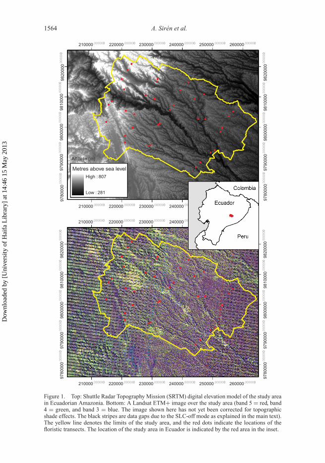
The study was carried out in a tropical rainforest in Ecuadorian Amazonia (Figure 1). Thestudy area is about 1300 km2, and it coincides with the study area of Sirén, Hambäck,and Machoa (2004), who studied hunting by the people of the Sarayaku community (1◦44′S, 77◦29′ W). There are no roads in the area, so all transport is by foot or river. Meanannual temperature in the area is about 23◦C, and the average annual precipitation is3000–3500 mm. Local inhabitants recognize a major rainy season in May–June, a dryseason in July–August, and a minor rainy season in December–January (Sirén 2004).Interannual variation in total rainfall, as well as variation in the timing of the seasons,is, however, high. The area is characterized by a rugged topography, which is shaped bytectonic uplift and landslides (Bès De Berc et al. 2005). The highest peaks in the north-west reach 640 m a.s.l., whereas in the southeast they do not surpass 500 m a.s.l. As theBobonaza River flows through the area, its elevation decreases from 390 to 330 m a.s.l.Occasionally, heavy rains cause flooding of the alluvial plains of the Bobonaza as well asof smaller rivers or creeks, but the water also withdraws rapidly, so there are no seasonallyflooded varzea forests in the area. Swamp forests with dense stands of Mauritia flexu-osa occur only as dispersed patches, the total area of which is negligible in comparisonwith the total forest area. Agricultural fields and anthropogenic secondary forests (fallows)cover about 4% of the total area and are concentrated near villages and navigable rivers(Sirén 2007). Small patches of natural secondary forest also exist as a result of landslidesor storms, but most of the area is covered by old-growth terra firme forest.
2.2. Field inventory
The sites for floristic transects were selected in such a way that they got fairly evenly dis-tributed throughout the study area (Figure 1). Whenever possible, transects were locatednear existing hunting trails, because travel through the forest in the absence of trails wasextremely slow. A total of 36 transects were established, and each transect was 2 m wideand 500 m long. In order to cover the full range of the topographic variation, two nearby
Dow
nloa
ded
by [
Uni
vers
ity o
f H
aifa
Lib
rary
] at
14:
46 1
5 M
ay 2
013
1564 A. Sirén et al.
210000,000000
9820
000,0
0000
098
1000
0,000
000
9800
000,0
0000
097
9000
0,000
000
9780
000,0
0000
098
2000
0,000
000
9810
000,0
0000
098
0000
0,000
000
9790
000,0
0000
097
8000
0,000
000
9820
000,0
0000
098
1000
0,000
000
9800
000,0
0000
097
9000
0,000
000
9780
000,0
0000
098
2000
0,000
000
9810
000,0
0000
098
0000
0,000
000
9790
000,0
0000
097
8000
0,000
000
220000,000000 230000,000000 240000,000000
210000,000000 220000,000000 230000,000000
240000,00
240000,00
210000,000000 220000,000000 230000,000000
250000,000000 260000,000000
210000,000000 220000,000000 230000,000000 240000,000000 250000,000000 260000,000000
Metres above sea levelHigh : 807
Altitude (m)
Low : 281
Figure 1. Top: Shuttle Radar Topography Mission (SRTM) digital elevation model of the study areain Ecuadorian Amazonia. Bottom: A Landsat ETM+ image over the study area (band 5 = red, band4 = green, and band 3 = blue. The image shown here has not yet been corrected for topographicshade effects. The black stripes are data gaps due to the SLC-off mode as explained in the main text).The yellow line denotes the limits of the study area, and the red dots indicate the locations of thefloristic transects. The location of the study area in Ecuador is indicated by the red area in the inset.
Dow
nloa
ded
by [
Uni
vers
ity o
f H
aifa
Lib
rary
] at
14:
46 1
5 M
ay 2
013
International Journal of Remote Sensing 1565
transects were always taken to represent different parts of the local topography. One transectstarted at a creek or a river and went upwards at an approximately right angle to the maindirection of the drainage network. The other transect started 50 m behind the top of a ridge,then passed the top of the ridge and continued downwards, approximately at a right angleto the main direction of the drainage network.
Each transect consisted of a narrow straight trail opened with a machete in the selectedcompass bearing. Transects were at first measured with a measuring tape, taking care tomeasure horizontally even in steep terrain, and georeferenced with a Garmin Etrex VistaCx GPS receiver (Garmin, Inc., Olathe, KS, USA). A Garmin Etrex Vista HCx receiverwas found to be more reliable and was later used both for georeferencing and for measuringtransect length.
Because floristic inventories in tropical rainforests are very laborious, pteridophytes(ferns and lycophytes) were used as indicators of floristic and edaphic patterns in thestudy area. Pteridophytes have three important advantages in this context. First, they arerelatively easy to observe, collect, and identify, which speeds up fieldwork and makes itpossible to inventory more transects. Second, they are relatively abundant but not exces-sively species rich, which facilitates obtaining robust sample sizes within the transects(Ruokolainen et al. 2007; Jones, Tuomisto, and Olivas 2008). Third, information on thedistribution of Amazonian pteridophytes along edaphic gradients already exists from othersites, which makes it possible to use pteridophyte species composition to infer edaphicproperties for a site.
For this purpose, a list of pteridophyte species was prepared for each transect. All ter-restrial individuals with at least one green leaf longer than 10 cm were considered, aswell as those epiphytic and climbing individuals that had such leaves below 2 m height.Although epiphytes have no direct connection with the soil, including them has been thecommon practice in these kinds of inventories (e.g. Tuomisto et al. 2003a, 2003b). This isbecause many species are able to grow both on the ground and epiphytically, and often itis difficult to establish whether a particular individual has a soil connection. All floristicsurveys were done by the same person (AS) with some training in identification of herbar-ium specimens but without previous experience of pteridophyte inventories in the field.Therefore, voucher specimens of all observed species were initially collected for identifi-cation by an expert on Ecuadorian ferns (HN). Based on photographs of these identifiedvoucher specimens, a simple photo guide was prepared and then used in the field for thesubsequent transects. Eventually, most species could be identified in the field, but voucherspecimens were nevertheless collected for verification. The time needed to survey a sin-gle 500 m transect was thus reduced from 5 days in the beginning to 2–4 h towards theend of fieldwork. All voucher specimens were finally identified by HT to ensure that thespecies concepts matched those used in Tuomisto, Ruokolainen, and Yli-Halla (2003). Thiswas necessary to calculate soil cation content optima for each pteridophyte species for thepurposes of calibration (to be described below).
2.3. Analyses of floristic data
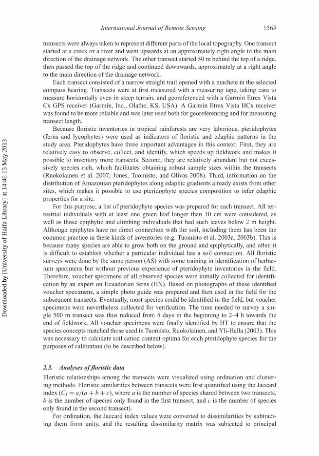
Floristic relationships among the transects were visualized using ordination and cluster-ing methods. Floristic similarities between transects were first quantified using the Jaccardindex (CJ = a/(a + b + c), where a is the number of species shared between two transects,b is the number of species only found in the first transect, and c is the number of speciesonly found in the second transect).
For ordination, the Jaccard index values were converted to dissimilarities by subtract-ing them from unity, and the resulting dissimilarity matrix was subjected to principal
Dow
nloa
ded
by [
Uni
vers
ity o
f H
aifa
Lib
rary
] at
14:
46 1
5 M
ay 2
013
1566 A. Sirén et al.
coordinates analysis (PCoA). This ordination method aims at concentrating informationfrom the dissimilarity matrix such that the compositional dissimilarities can be visualizedusing just a few dimensions. Clustering of the transects was carried out using the pro-portional link linkage algorithm. This is a hierarchical agglomerative clustering methodthat joins transects into groups on the basis of their pairwise floristic similarity (here itis based on the Jaccard index). Connectedness was set at 0.5 (i.e. midway between sin-gle and complete linkages; Legendre and Legendre 1998). The clustering results provideinsights into the compositional data that are complementary to those obtained by ordination.These analyses together provide the background information needed for making inferencesconcerning environmental variation in the study area.
Soil cation content in the transects was estimated using calibration, which is a standardmethod in ecology (Jongman, Ter Braak, and Van Tongeren 1995). Calibration is based onthe idea that any one plant species only occurs in a part of any environmental gradient, andthat its occurrence is most frequent and its abundance highest at sites that are closest to itsoptimum conditions. Species optima for a given environmental variable can be estimatedas an average of the variable values in the sites where the species have been observed.The value of the variable at a new site can then be estimated as an average of the optimaof those species that occur at the site. For this purpose, soil cation content optima forthe pteridophyte species occurring in our transects were first calculated using data from134 other transects situated in Ecuador, Colombia, and northern Peru. These transects hadbeen established using a method similar to ours, but both pteridophyte species compositionand soil cation content data were available (Tuomisto, Ruokolainen, and Yli-Halla 2003and unpublished data). Those species observed in this study but not in the previous oneswere excluded from this analysis. For each species, its soil cation optimum was calculatedas a weighted arithmetic mean of the soil cation content in the transects where the specieshad been observed, with species abundance (number of individuals) in each transect usedas the weight. The optima were then used to estimate soil cation content for each transectof this study by calculating the mean of the optima of all those species that occurred in thetransect in question. This mean was unweighted because species abundance informationwas not collected in this study. The resulting numbers are here referred to as ‘calibratedsoil values’.
2.4. Estimation of soil values based on image data
For image interpretation, a Landsat Enhanced Thematic Mapper Plus (ETM+) image (path9, row 61) acquired on 2 July 2005 was used (Figure 1). This image was in scan linecorrector (SLC)-off mode, implying that there were data gaps due to a technical problemof the satellite sensor. Fortunately, the study area was at the centre of the scene, wherethe least number of data gaps are present. Both such SLC-off data gaps and pixels rep-resenting water or river beaches were masked out prior to image analysis. Radiometriccalibration of the image data to convert digital number (DN) values to physical at-sensorradiance was done according to Green, Schweik, and Hanson (2002). A number of pro-cedures for atmospheric and topographic correction were tested. The best performancewas achieved by combining atmospheric correction using the dark object subtractionand topographic correction method and by applying the equal area normalization algo-rithm of Erdas Imagine (Intergraph, Corp., Huntsville, AL, USA), also called the internalaverage relative (IAR) reflectance (Kruse 1988; Zamudio and Atkinson 1990), to eachpixel. A detailed comparison of different preprocessing procedures will be presentedelsewhere.
Dow
nloa
ded
by [
Uni
vers
ity o
f H
aifa
Lib
rary
] at
14:
46 1
5 M
ay 2
013
International Journal of Remote Sensing 1567
The spectral signatures in the satellite image and the calibrated soil values for thetransects were used to obtain a regression equation to estimate soil values over the entirestudy area. To collect spectral signatures, the GPS points of each 500 m floristic transectwere displayed on screen, and a 200 m × 600 m rectangle was placed on top of eachtransect. An average spectral signature was registered for each rectangle using Landsatbands 1–5 and 7. Multiple regression was then performed to model the calibrated soil val-ues as a linear function of spectral signatures in the six bands. Stepwise multiple regressionwas used in order to exclude from the regression equation those bands that did not have astatistically significant contribution to explaining the variation in the calibrated soil values(with criteria p ≤ 0.05 for entry and p ≥ 0.10 for removal).
Before using the regression equation to extrapolate soil values to the whole image,some additional image processing was done. Existing information on land use in the area(Sirén 2007; Sirén and Brondizio 2009) was used to mask out areas that were known orsuspected to be cultivated land or anthropogenic secondary forests (fallows). The land-usemask included all land within a 50 m buffer around pixels classified as cultivated land in1987 or as fallows in either 1987 or 2001; a 150 m buffer around pixels classified as culti-vated land in 2001; and a 200 m buffer around navigable rivers. After the land-use mask,a focal mean filter was applied to the image in order to remove such variation on a smallspatial scale, which is likely to represent noise rather than relevant ecological informa-tion. This filter was given a radius of 195 m, such that its area was approximately equalto that of the rectangles used to collect spectral signatures. Applying the focal mean filteralso filled the data gaps caused by the SLC-off mode. A side effect was that even pixelsthat had previously been excluded with the land-use mask were again given DN values,but these were eliminated by a second application of the land-use mask. An estimatedsoil value was then calculated for each pixel in the scene using the multiple regressionequation.
The error in the soil values estimated from the Landsat data in relation to the orig-inal soil values obtained by calibration was quantified by leave-one-out cross-validation.In this validation method, one transect is set aside to be used as the test set, and the remain-ing 35 transects are used as the training set to parameterize the regression equation. Eachtransect is then used as the test set in turn, and the estimated soil values obtained in this wayfor the test transects are compared with the original calibrated soil values. This provides ameasure of the expected accuracy of the results when the regression equation is appliedover the entire Landsat scene.
3. Results
3.1. Ordination, clustering, and calibrated soil values
The total number of pteridophyte species observed in the 36 transects was 182, but someclosely related species were confused in the field and were consequently lumped. Thenumerical analyses were therefore run with 171 broadly circumscribed species (gammarichness Rγ = 171 species). On average, the transects contained 46 species (alpha richnessRα = 46 species/transect). Rγ is 3.7 times as large as Rα, which indicates that the amountof compositional heterogeneity (beta richness Rβ) in the data corresponds to what wouldbe observed among 3.7 transects that share no species. The pairwise Jaccard index similar-ity values that were calculated between transects ranged between 0.13 and 0.65, with theaverage being 0.37.
PCoA showed that there is a strong compositional gradient in the floristic data. Thisis mainly captured along Axis 1, but there is also indication of an arch (transects at both
Dow
nloa
ded
by [
Uni
vers
ity o
f H
aifa
Lib
rary
] at
14:
46 1
5 M
ay 2
013
1568 A. Sirén et al.
–0.4
0.2
0
–0.2
0.2
Calibrated soil value3.3 – 4.34.3 – 5.35.3 – 6.36.3 – 7.3
7.3 – 8.3
8.3 – 9.3
210000,000000
9820
000,0
0000
098
1000
0,000
000
9800
000,0
0000
097
9000
0,000
000
9780
000,0
0000
0
9820
000,0
0000
098
1000
0,000
000
9800
000,0
0000
097
9000
0,000
000
9780
000,0
0000
0
220000,000000 230000,000000 240000,000000 250000,000000 260000,000000
210000,000000 220000,000000 230000,000000 240000,000000 250000,000000 260000,000000
0
–0.2
–0.2 0 0.2
–0.4 –0.2
3.3 – 4.3
Calibrated soil value
4.3 – 5.3
5.3 – 6.3
6.3 – 7.3
7.3 – 8.3
8.3 – 9.3
Rivers
Villages
Limits of study area
0 5 10 20 30 40km
0 0.2
Figure 2. Top: The positions of 36 transects of 2 m × 500 m along the first two axes of PCoAbased on floristic differences of pteridophytes (one-complement of the Jaccard index). Bottom: Thegeographical distribution of the same 36 transects in the study area in Ecuadorian Amazonia. In bothpanels, the size of the circle corresponding to each transect is proportional to the calibrated soilvalue (estimated using floristic data), and the colours indicate to which of seven recognized floristicclasses each transect belongs (proportional link linkage clustering with connectedness 0.5 based onthe Jaccard index).
Dow
nloa
ded
by [
Uni
vers
ity o
f H
aifa
Lib
rary
] at
14:
46 1
5 M
ay 2
013
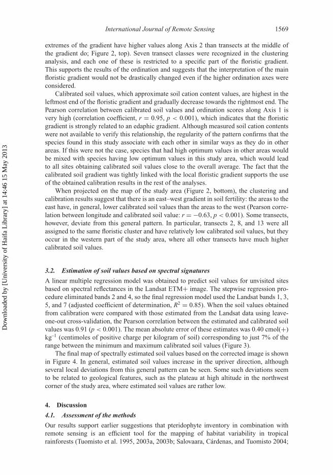
International Journal of Remote Sensing 1569
extremes of the gradient have higher values along Axis 2 than transects at the middle ofthe gradient do; Figure 2, top). Seven transect classes were recognized in the clusteringanalysis, and each one of these is restricted to a specific part of the floristic gradient.This supports the results of the ordination and suggests that the interpretation of the mainfloristic gradient would not be drastically changed even if the higher ordination axes wereconsidered.
Calibrated soil values, which approximate soil cation content values, are highest in theleftmost end of the floristic gradient and gradually decrease towards the rightmost end. ThePearson correlation between calibrated soil values and ordination scores along Axis 1 isvery high (correlation coefficient, r = 0.95, p < 0.001), which indicates that the floristicgradient is strongly related to an edaphic gradient. Although measured soil cation contentswere not available to verify this relationship, the regularity of the pattern confirms that thespecies found in this study associate with each other in similar ways as they do in otherareas. If this were not the case, species that had high optimum values in other areas wouldbe mixed with species having low optimum values in this study area, which would leadto all sites obtaining calibrated soil values close to the overall average. The fact that thecalibrated soil gradient was tightly linked with the local floristic gradient supports the useof the obtained calibration results in the rest of the analyses.
When projected on the map of the study area (Figure 2, bottom), the clustering andcalibration results suggest that there is an east–west gradient in soil fertility: the areas to theeast have, in general, lower calibrated soil values than the areas to the west (Pearson corre-lation between longitude and calibrated soil value: r = −0.63, p < 0.001). Some transects,however, deviate from this general pattern. In particular, transects 2, 8, and 13 were allassigned to the same floristic cluster and have relatively low calibrated soil values, but theyoccur in the western part of the study area, where all other transects have much highercalibrated soil values.
3.2. Estimation of soil values based on spectral signatures
A linear multiple regression model was obtained to predict soil values for unvisited sitesbased on spectral reflectances in the Landsat ETM+ image. The stepwise regression pro-cedure eliminated bands 2 and 4, so the final regression model used the Landsat bands 1, 3,5, and 7 (adjusted coefficient of determination, R2 = 0.85). When the soil values obtainedfrom calibration were compared with those estimated from the Landsat data using leave-one-out cross-validation, the Pearson correlation between the estimated and calibrated soilvalues was 0.91 (p < 0.001). The mean absolute error of these estimates was 0.40 cmol(+)kg–1 (centimoles of positive charge per kilogram of soil) corresponding to just 7% of therange between the minimum and maximum calibrated soil values (Figure 3).
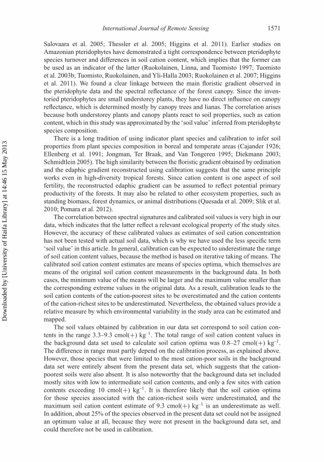
The final map of spectrally estimated soil values based on the corrected image is shownin Figure 4. In general, estimated soil values increase in the upriver direction, althoughseveral local deviations from this general pattern can be seen. Some such deviations seemto be related to geological features, such as the plateau at high altitude in the northwestcorner of the study area, where estimated soil values are rather low.
4. Discussion
4.1. Assessment of the methods
Our results support earlier suggestions that pteridophyte inventory in combination withremote sensing is an efficient tool for the mapping of habitat variability in tropicalrainforests (Tuomisto et al. 1995, 2003a, 2003b; Salovaara, Cárdenas, and Tuomisto 2004;
Dow
nloa
ded
by [
Uni
vers
ity o
f H
aifa
Lib
rary
] at
14:
46 1
5 M
ay 2
013
1570 A. Sirén et al.
0
2
4
6
8
10
0 2 4 6 8 10
Estimated soil value (spectral)
Cal
ibra
ted
soil
valu
e (f
loris
tic)
Figure 3. Calibrated soil values plotted against estimated soil values. Estimated soil values arecalculated using multiple regression of calibrated soil values against spectral reflectances on anatmospherically and topographically corrected Landsat ETM+ satellite image using leave-one-outcross-validation. Each point represents one field transect site.
200000,000000
9820
000,0
0000
098
1000
0,000
000
9800
000,0
0000
097
9000
0,000
000
9820
000,0
0000
098
1000
0,000
000
9800
000,0
0000
097
9000
0,000
000
210000,000000 220000,000000 230000,000000 240000,000000
N
250000,000000 260000,000000
200000,000000 210000,000000 220000,000000 230000,000000 240000,000000 250000,000000 260000,000000
3.3–4.3
Below 3.3
Estimated soil value
4.3–5.3
5.3–6.3
6.3–7.3
7.3–8.3
8.3–9.3
Above 9.3
0 5 10 20 30 40 50km
Figure 4. Map of estimated soil values in the study area in Ecuadorian Amazonia. The soil valuesprovide an approximation of the concentration of exchangeable bases in the soil (Ca, K, Mg, and Nain cmol(+) kg–1). Estimated values were obtained with a multiple linear regression, where spectralvalues of Landsat ETM+ bands 1, 3, 5, and 7 were used as the independent variables. The regressionequation was parameterized with soil values obtained from calibration, i.e. on the basis of pterid-pohyte species composition in 36 field transects. All calibrated soil values were within the range3.3–9.3 cmol(+) kg–1, so estimated values outside this range need to be interpreted with caution.
Dow
nloa
ded
by [
Uni
vers
ity o
f H
aifa
Lib
rary
] at
14:
46 1
5 M
ay 2
013
International Journal of Remote Sensing 1571
Salovaara et al. 2005; Thessler et al. 2005; Higgins et al. 2011). Earlier studies onAmazonian pteridophytes have demonstrated a tight correspondence between pteridophytespecies turnover and differences in soil cation content, which implies that the former canbe used as an indicator of the latter (Ruokolainen, Linna, and Tuomisto 1997; Tuomistoet al. 2003b; Tuomisto, Ruokolainen, and Yli-Halla 2003; Ruokolainen et al. 2007; Higginset al. 2011). We found a clear linkage between the main floristic gradient observed inthe pteridophyte data and the spectral reflectance of the forest canopy. Since the inven-toried pteridophytes are small understorey plants, they have no direct influence on canopyreflectance, which is determined mostly by canopy trees and lianas. The correlation arisesbecause both understorey plants and canopy plants react to soil properties, such as cationcontent, which in this study was approximated by the ‘soil value’ inferred from pteridophytespecies composition.
There is a long tradition of using indicator plant species and calibration to infer soilproperties from plant species composition in boreal and temperate areas (Cajander 1926;Ellenberg et al. 1991; Jongman, Ter Braak, and Van Tongeren 1995; Diekmann 2003;Schmidtlein 2005). The high similarity between the floristic gradient obtained by ordinationand the edaphic gradient reconstructed using calibration suggests that the same principleworks even in high-diversity tropical forests. Since cation content is one aspect of soilfertility, the reconstructed edaphic gradient can be assumed to reflect potential primaryproductivity of the forests. It may also be related to other ecosystem properties, such asstanding biomass, forest dynamics, or animal distributions (Quesada et al. 2009; Slik et al.2010; Pomara et al. 2012).
The correlation between spectral signatures and calibrated soil values is very high in ourdata, which indicates that the latter reflect a relevant ecological property of the study sites.However, the accuracy of these calibrated values as estimates of soil cation concentrationhas not been tested with actual soil data, which is why we have used the less specific term‘soil value’ in this article. In general, calibration can be expected to underestimate the rangeof soil cation content values, because the method is based on iterative taking of means. Thecalibrated soil cation content estimates are means of species optima, which themselves aremeans of the original soil cation content measurements in the background data. In bothcases, the minimum value of the means will be larger and the maximum value smaller thanthe corresponding extreme values in the original data. As a result, calibration leads to thesoil cation contents of the cation-poorest sites to be overestimated and the cation contentsof the cation-richest sites to be underestimated. Nevertheless, the obtained values provide arelative measure by which environmental variability in the study area can be estimated andmapped.
The soil values obtained by calibration in our data set correspond to soil cation con-tents in the range 3.3–9.3 cmol(+) kg–1. The total range of soil cation content values inthe background data set used to calculate soil cation optima was 0.8–27 cmol(+) kg–1.The difference in range must partly depend on the calibration process, as explained above.However, those species that were limited to the most cation-poor soils in the backgrounddata set were entirely absent from the present data set, which suggests that the cation-poorest soils were also absent. It is also noteworthy that the background data set includedmostly sites with low to intermediate soil cation contents, and only a few sites with cationcontents exceeding 10 cmol(+) kg–1. It is therefore likely that the soil cation optimafor those species associated with the cation-richest soils were underestimated, and themaximum soil cation content estimate of 9.3 cmol(+) kg–1 is an underestimate as well.In addition, about 25% of the species observed in the present data set could not be assignedan optimum value at all, because they were not present in the background data set, andcould therefore not be used in calibration.
Dow
nloa
ded
by [
Uni
vers
ity o
f H
aifa
Lib
rary
] at
14:
46 1
5 M
ay 2
013
1572 A. Sirén et al.
4.2. Applications
To successfully protect biodiversity, conservation area networks need to include a sufficientrepresentation of the entire range of habitat variability in all regions. Broad-scale mapsof environmental and floristic variation are needed to assess how well this goal has beenreached and to identify areas that should be prioritized in future conservation actions. Themethod used in this article provides one means to produce such maps.
The estimation of soil characteristics could also be used in land-use planning in orderto direct agricultural development to fertile areas. This would help avoiding such errors ashave been done in the past, when agricultural expansion has been targeted to areas wheresoils have been too poor for the intended crops (e.g. Fearnside 1986). At the same time,the method may be proactively used by conservationists to identify forests that may be atincreased risk of conversion to agriculture due to their high soil fertility.
Since general forest productivity is affected by soil properties, understanding theheterogeneity in soils is also important for estimating sustainable levels for the harvest-ing of forest products such as timber or game animals. Earlier studies have found that gameanimal abundance (as estimated from catch per unit of hunting effort) is spatially variablein our study area (Sirén, Hambäck, and Machoa 2004 and unpublished data). Human hunt-ing effort itself explained much of this variability for all important game species, but otherfactors seemed to complicate the picture. This study was motivated by the need to find outwhether mammal abundance varies naturally in response to variability in soil productivity,not just as a result of human hunting pressure. The map of estimated soil values producedhere (Figure 4) will provide the means to test this hypothesis. The local community is con-cerned about the sustainability of hunting in its territory and has set aside no-take areasfor wildlife in order to ensure long-term sustainability of hunting (Sirén 2006). Even whenintentions are good, however, failure to recognize spatial variability of wildlife habitats maylead to suboptimal harvest strategies and put sustainability at risk (Jonzén, Lundberg, andGårdmark 2001). Spatial information on environmental variability, and on how game pop-ulations react to this variability, may be useful when deciding about the location and sizeof no-take areas, as well as when evaluating their performance.
The United Nations Reduced Emissions from Deforestation and Degradation (REDD)programme aims to establish mechanisms for monetary compensation for maintaining car-bon stocks in forests. In the southern part of Peruvian Amazonia, it has been found thatcarbon stocks vary considerably both among and within 25 mainly topographically definedforest types (Asner et al. 2010). Soil properties can be expected to be among the ulti-mate determinants of carbon stocks, but the exact relationships are not yet well understood(Laurence et al. 1999; Clark and Clark 2000; Quesada et al. 2009). Including informationon edaphic characteristics, either directly by soil chemical analyses or indirectly by floristicinventory of indicator species, can therefore be expected to improve the accuracy of themodels used to estimate carbon stocks over large areas.
AcknowledgementsDuring the early planning phase of the project, Anders Sirén was funded by the Academy ofFinland. During further planning, as well as fieldwork and preliminary data analysis, he was fundedby a postdoc grant from the Swedish International Development Authority (SIDA) and a postdocgrant from the Swedish Research Council for Environment, Agricultural Sciences, and SpatialPlanning (FORMAS). During the final analyses and writing the manuscript, Sirén was funded byAkademikernas Erkända Arbetslöshetskassa, the Swedish Cultural Fund in Finland, the Oscar ÖflundFoundation, and by a grant awarded to Professor Risto Kalliola by the Kone Foundation. Saul Malaver,Alex Machoa, and Angel Gualinga assisted with fieldwork. We thank the Government Council of the
Dow
nloa
ded
by [
Uni
vers
ity o
f H
aifa
Lib
rary
] at
14:
46 1
5 M
ay 2
013
International Journal of Remote Sensing 1573
Sarayaku Community for facilitating fieldwork and Dra. Laura Arcos Terán, Dean of the Natural andExact Sciences, Faculty of the Pontificia Universidad Católica del Ecuador, for institutional supportto the development of the project.
ReferencesAsner, G. P., G. V. N. Powell, J. Mascaro, D. E. Knapp, J. K. Clark, J. Jacobson, T. Kennery-Bowdoin,
A. Blaji, G. Paez-Acosta, E. Victoria, L. Secada, M. Valqui, and R. F. Hughes. 2010. “High-Resolution Forest Carbon Stocks and Emissions in the Amazon.” PNAS 107: 16738–42.
Bès De Berc S., J. C. Soula, P. Baby, M. Souris, F. Christophoul, and J. Rosero. 2005. “GeomorphicEvidence of Active Deformation and Uplift in a Modern Continental Wedge-Top-ForedeepTransition: Example of the Eastern Ecuadorian Andes.” Tectonophysics 399: 351–80.
Cajander, A. K. 1926. “The Theory of Forest Types.” Acta Forestalia Fennica 29: 1–108.Clark, D. B., and D. A. Clark. 2000. “Landscape Variation in Forest Structure and Biomass in a
Tropical Rain Forest.” Forest Ecology and Management 137: 185–98.Coley, P. D., J. P. Bryant, and F. S. Chapin III. 1985. “Resource Availability and Plant Antiherbivore
Defence.” Science 230: 895–9.Diekmann, M. 2003. “Species Indicator Values as an Important Tool in Applied Plant Ecology: A
Review.” Basic and Applied Ecology 4: 493–506.Duivenvoorden, J. F. 1995. “Tree Species Composition and Rain Forest-Environment Relationships
in the Middle Caquetá Area, Colombia, NW Amazonia.” Vegetation 120: 91–113.Duque, A., M. Sánchez, J. Cavelier, and J. Duivenvoorden. 2002. “Different Floristic Patterns of
Woody Understorey and Canopy Plants in Colombian Amazonia.” Journal of Tropical Ecology18: 499–525.
Duque, A. J., J. F. Duivenvoorden, J. Cavelier, M. Sánchez, C. Polanía, and A. León. 2005. “Fernsand Melastomataceae as Indicators of Vascular Plant Composition in Rain Forests of ColombianAmazonia.” Plant Ecology 178: 1–13.
Ellenberg, H., H. E. Weber, R. Düll, V. Wirth, W. Werner, and D. Paulissen. 1991. “Zeigerwerte VonPflanzen in Mitteleuropa.” Scripta Geobotanica 18: 1–248.
Fearnside, P. 1986. “Settlement in Rondônia and the Token Role of Science and Technology inBrazil’s Amazonian Development.” Interciencia 11: 229–36.
Gao, Y., and W. Zhang. 2009. “A Simple Empirical Correction Method for ETM+ Imagery.”International Journal of Remote Sensing 30: 2259–75.
Gartlan, S. J., D. B. Mckey, P. G. Waterman, C. N. Mbi, and T. T. Struhsaker. 1980. “A ComparativeStudy of the Phytochemistry of Two African Rain Forests.” Biochemical Systematics and Ecology8: 401–22.
Gentry, A. H. 1988. “Changes in Plant Community Diversity and Floristic Composition onEnvironmental and Geographical Gradients.” Annals of the Missouri Botanical Garden 75:1–34.
Green, G. M., C. Schweik, and M. Hanson 2002. “Radiometric Calibration of LANDSAT Multi-spectral Scanner and Thematic Mapper Images: Guidelines for the Global Change Community.”CWP-02-03, Center for the Study of Institutions, Population, and Environmental Change(CIPEC), Indiana University, Bloomington.
Higgins, M. A., K. Ruokolainen, H. Tuomisto, N. Llerena, G. Cardenas, O. L. Phillips, R. Vásquez,and M. Räsänen. 2011. “Geological Control of Floristic Composition in Amazonian Forests.”Journal of Biogeography 38: 2136–49.
Honorio Coronado, E. N., T. R. Baker, O. L. Phillips, N. C. A. Pitman, R. T. Pennington, R. VasquezMartinez, A. Monteagudo, H. Mogollon, N. Davila Cardozo, M. Rios, R. Garcia-Villacorta,E. Valderrama, M. Ahuite, I. Huamantupa, D. A. Neill, W. F. Laurance, H. E. M. Nascimento,S. S. De Almeida, T. J. Killeen, L. Arroyo, P. Nunez, and L. Freitas Alvarado. 2009. “Multi-Scale Comparisons of Tree Composition in Amazonian Terra Firme Forests.” Biogeosciences 6:2719–31.
IBGE (Instituto Brasileiro de Geografia e Estatística). 2004. Mapa de Vegetação do Brasil. 3rd ed. Riode Janeiro: Instituto Brasileiro de Geografia e Estatística. ftp://ftp.ibge.gov.br/Cartas_e_Mapas/Mapas_Murais/.
Janzen, D. H. 1974. “Tropical Blackwater Rivers, Animals, and Mast Fruiting by theDipterocarpaceae.” Biotropica 6: 69–103.
Dow
nloa
ded
by [
Uni
vers
ity o
f H
aifa
Lib
rary
] at
14:
46 1
5 M
ay 2
013
1574 A. Sirén et al.
Jones, M. M., H. Tuomisto, and P. C. Olivas. 2008. “Differences in the Degree of EnvironmentalControl on Large and Small Tropical Plants: Just a Sampling Effect?” Journal of Ecology 96:367–77.
Jongman, R. H. G., C. J. F. Ter Braak, and O. F. R. Van Tongeren, eds. 1995. Data Analysis inCommunity and Landscape Ecology, 299. Cambridge: Cambridge University Press.
Jonzén, N., P. Lundberg, and A.Gårdmark. 2001. “Harvesting Spatially Distributed Populations.”Wildlife Biology 7: 197–203.
Kruse, F. A. 1988. “Use of Airborne Imaging Spectrometer Data to Map Minerals Associated withHydrotehermally Altered Rocks in the Northern Grapevine Mts., Nevada and California.” RemoteSensing of Environment 24: 31–51.
Laurance, W. F., P. M. Fearnside, S. G. Laurance, P. Delamonica, T. E. Lovejoy, J. M. Rankin-DeMerona, J. Q. Chambers, and C. Gascon. 1999. “Relationship Between Soils and Amazon ForestBiomass: A Landscape-Scale Study.” Forest Ecology and Management 118: 127–38.
Legendre, P., and L. Legendre. 1998. Numerical Ecology, Second English Edition (Developments inEnvironmental Modelling, vol. 20). Amsterdam: Elsevier.
Lu, D., P. Mausel, E. Brondizio, and E. Moran. 2003. “Classification of Successional Forest Stages inthe Brazilian Amazon Basin.” Forest Ecology and Management 181: 301–12.
Lu, D., E. Moran, and M. Batistella. 2003. “Linear Mixture Model Applied to Amazonian VegetationClassification.” Remote Sensing of Environment 87: 456–69.
Phillips, O. L., P. Nuñez Vargas, A. Lorenzo Monteagudo, A. Peña Cruz, M.-E. Chuspe Zans,W. Galiano Sanchez, M. Yli-Halla, and S. Rose. 2003. “Habitat Association Among AmazonianTree Species: A Landscape-Scale Approach.” Journal of Ecology 91: 757–75.
Pomara, L. Y., K. Ruokolainen, H. Tuomisto, and K. Young. 2012. “Avian Composition Co-varieswith Floristic Composition and Soil Nutrient Concentration in Amazonian Upland Forests.”Biotropica 44: 545–53.
Quesada, C. A., J. Lloyd, M. Schwartz, T. R. Baker, O. L. Phillips, S. Patiño, C. Czimczik,M. G. Hodnett, R. Herrera, A. Arneth, G. Lloyd, Y. Malhi, N. Dezzeo, F. J. Luizão, A. J. B. Santos,J. Schmerler, L. Arroyo, M. Silveira, N. Priante Filho, E. M. Jimenez, R. Paiva, I. Vieira,D. A. Neill, N. Silva, M. C. Peñuela, A. Monteagudo, R. Vásquez, A. Prieto, A. Rudas,S. Almeida, N. Higuchi, A. T. Lezama, G. López-González, J. Peacock, N. M. Fyllas, E. AlvarezDávila, T. Erwin, A. di Fiore, K. J. Chao, E. Honorio, T. Killeen, A. Peña Cruz, N. Pitman,P. Núñez Vargas, R. Salomão, J. Terborgh, and H. Ramírez. 2009. “Regional and Large-ScalePatterns in Amazon Forest Structure and Function Are Mediated by Variations in Soil Physicaland Chemical Properties.” Biogeosciences 6: 3993–4057.
Riaño, D., E. Chuvieco, J. Salas, and I. Aguado. 2003. “Assessment of Different TopographicCorrections in Landsat-TM Data for Mapping Vegetation Types.” IEEE Transactions onGeoscience and Remote Sensing 41: 1056–61.
Ruokolainen, K., A. Linna, and H. Tuomisto. 1997. “Use of Melastomataceae and Pteridophytes forRevealing Phytogeographic Patterns in Amazonian Rain Forests.” Journal of Tropical Ecology13: 243–56.
Ruokolainen, K., H. Tuomisto, M. J. Macía, M. A. Higgins, and M. Yli-Halla. 2007. “Are Floristicand Edaphic Patterns in Amazonian Rain Forests Congruent for Trees, Pteridophytes andMelastomataceae?” Journal of Tropical Ecology 23: 13–25.
Salovaara, K. J. 2005. “Habitat Heterogeneity and the Distribution of Large-Bodied Mammals inPeruvian Amazonia.” Report No. 53, Department of Biology, University of Turku, Finland.
Salovaara, K. J., G. G. Cárdenas, and H. Tuomisto. 2004. “Forest Classification in an AmazonianRainforest Landscape Using Pteridophytes as Indicator Species.” Ecography 27: 689–700.
Salovaara, K., S. Thessler, and R. N. Malik, and H. Tuomisto. 2005. “Classification of AmazonianPrimary Rain Forest Vegetation Using Landsat ETM+ Satellite Imagery.” Remote Sensing ofEnvironment 97: 39–51.
Schmidtlein, S. 2005. “Imaging Spectroscopy as a Tool for Mapping Ellenberg Indicator Values.”Journal of Applied Ecology 42: 966–74.
Sirén, A. 2004. “Changing Interactions Between Humans and Nature in Sarayaku, EcuadorianAmazon.” Acta Universitatis Agriculturae Sueciae, Agraria, 447. Uppsala: Swedish Universityof Agricultural Sciences.
Sirén, A. H. 2006. “Natural Resources in Indigenous People’s Lands in Amazonia: A Tragedy of theCommons?” International Journal of Sustainable Development & World Ecology 13: 363–74.
Dow
nloa
ded
by [
Uni
vers
ity o
f H
aifa
Lib
rary
] at
14:
46 1
5 M
ay 2
013

International Journal of Remote Sensing 1575
Sirén, A. H. 2007. “Population Growth and Land Use Intensification in a Subsistence-BasedIndigenous Community in the Amazon.” Human Ecology 35: 669–80.
Sirén, A. H., and E. S. Brondizio. 2009. “Detecting Subtle Land Use Change in Tropical Forests.”Applied Geography 29: 201–11.
Sirén, A., P. Hambäck, and J. Machoa. 2004. “Including Spatial Heterogeneity and Animal DispersalWhen Evaluating Hunting: A Model Analysis and an Empirical Assessment in an AmazonianCommunity.” Conservation Biology 18: 1315–29.
Slik, J. W. F., S.-I. Aiba, F. Q. Brearley, C. H. Cannon, O. Forshed, K. Kitayama, H. Nagamasu,R. Nilus, J. Payne, G. Paoli, A. D. Poulsen, N. Raes, D. Sheil, K. Sidiyasa, E. Suzuki, andJ. L. C. H. Van Valkenburg. 2010. “Environmental Correlates of Tree Biomass, Basal Area, WoodSpecific Gravity and Stem Density Gradients in Borneo’s Tropical Forests.” Global Ecology andBiogeography 19: 50–60.
Thessler, S., K. Ruokolainen, H. Tuomisto, and E. Tomppo. 2005. “Mapping Gradual Landscape-Scale Floristic Changes in Amazonian Primary Rain Forests by Combining Ordination andRemote Sensing.” Global Ecology and Biogeography 14: 315–25.
Thessler, S., S. Sesnie, Z. S. Ramos Bendaña, K. Ruokolainen, E. Tomppo, and B. Finegan. 2008.“Using k-Nn and Discriminant Analyses to Classify Rain Forest Types in a Landsat TM ImageOver Northern Costa Rica.” Remote Sensing of Environment 112: 2485–94.
Tuomisto, H., A. D. Poulsen, K. Ruokolainen, R. C. Moran, C. Quintana, J. Celi, and G. Cañas.2003a. “Linking Floristic Patterns with Soil Heterogeneity and Satellite Imagery in EcuadorianAmazonia.” Ecological Applications 13: 352–71.
Tuomisto, H., K. Ruokolainen, M. Aguilar, and A. Sarmiento. 2003b. “Floristic Patterns Along a43-km Long Transect in an Amazonian Rain Forest.” Journal of Ecology 91: 743–56.
Tuomisto, H., K. Ruokolainen, R. Kalliola, A. Linna, W. Danjoy, and Z. Rodriguez. 1995. “DissectingAmazonian Biodiversity.” Science 269: 63–6.
Tuomisto, H., K. Ruokolainen, A. D. Poulsen, R. C. Moran, C. Quintana, G. Cañas, and J. Celi. 2002.“Distribution and Diversity of Pteridophytes and Melastomataceae Along Edaphic Gradients inYasuni National Park, Ecuadorian Amazonia.” Biotropica 34: 516–33.
Tuomisto, H., K. Ruokolainen, and M. Yli-Halla. 2003. “Dispersal, Environment, and FloristicVariation of Western Amazonian Forests.” Science 299: 241–4.
Twele, A., and S. Erasmi. 2005. “Evaluating Topographic Correction Algorithms for Improved LandCover Discrimination in Mountainous Areas of Central Sulawesi.” In Remote Sensing and GISfor Environmental Studies, Göttinger Geographische Abhandlungen 113, edited by S. Erasmi,B. Cyffka, and M. Kappas, 287–95. Göttingen: Geographischen Instituts der UniversitätGöttingen.
Vieira, I. C. G., S. De Almeida, A. Davidson, E. A. Stone, T. A. Reis, C. J. De Carvalho, and J.B. Guerrero. 2003. “Classifying Successional Forests Using Landsat Spectral Properties andEcological Characteristics in Eastern Amazonia.” Remote Sensing of Environment 87: 470–81.
Vormisto, J., O. L. Phillips, K. Ruokolainen, H. Tuomisto, and R.Vásquez. 2000. “A Comparison ofFine-Scale Distribution Patterns of Four Plant Groups in an Amazonian Rainforest.” Ecography23: 349–59.
Vormisto, J., J. C. Svenning, P. Hall, and H. Balslev. 2004. “Diversity and Dominance in Palm(Arecaceae) Communities in Terra Firme Forests in the Western Amazon Basin.” Journal ofEcology 92: 577–88.
Zamudio, J. A., and W. W. Atkinson. 1990. “Analysis of AVIRIS Data for Spectral Discrimination ofGeologic Materials in the Dolly Varden Mountains.” In Paper presented at the Second AirborneVisible Infrared Imaging Sepctrometer (AVIRIS) Conference, Pasadena, CA, June 1990, 162–6.Pasadena, CA: Jet Propulsion Laboratory (JPL) Publication 90-54.
Zuquim, G., F. R. C. Costa, J. Prado, and R. Braga-Neto. 2009. “Distribution of PteridophyteCommunities Along Environmental Gradients in Central Amazonia, Brazil.” Biodiversity andConservation 18: 151–66.
Dow
nloa
ded
by [
Uni
vers
ity o
f H
aifa
Lib
rary
] at
14:
46 1
5 M
ay 2
013