8/15/2017

1

Where You Are!

Economics 305 – Macroeconomic Theory

M and W from 12:00pm to 12:50pm

Text: Gregory Mankiw: Macroeconomics, Worth, 9th, 8th edition.

A used copy of 8th edition is good.

Course Webpage

http://www.terpconnect.umd.edu/~jneri/Econ305

NOTE: upper-case E

Who am I ?

Dr. John Neri

Office: Morrill Hall, Room 1106D,

M and W 10:30am to 11:30am

Syllabus

8/15/2017

2

https://www.c-span.org/video/?430765-

1/federal-reserve-chair-predicts-moderate-

pace-economic-growth

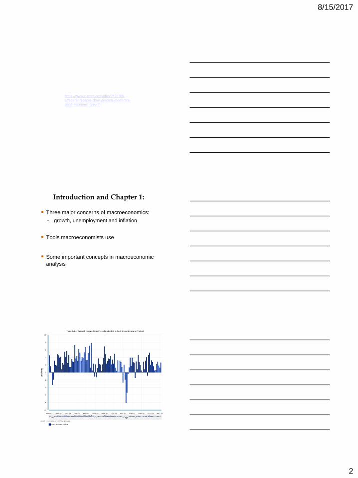
Introduction and Chapter 1:

Three major concerns of macroeconomics:

- growth, unemployment and inflation

Tools macroeconomists use

Some important concepts in macroeconomic

analysis

8/15/2017

3

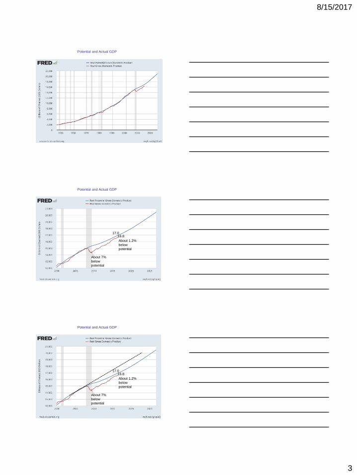
Potential and Actual GDP

About 7%

below

potential

About 1.2%

below

potential

Potential and Actual GDP

17.0 16.8

About 7%

below

potential

About 1.2%

below

potential

Potential and Actual GDP

17.0 16.8

8/15/2017

4

Long-term Real GDP Per Capita (2000 dollars)

long-run upward trend…

Great

Depression

World War II

First oil

price shock

Second oil

price shock

9/11/2001

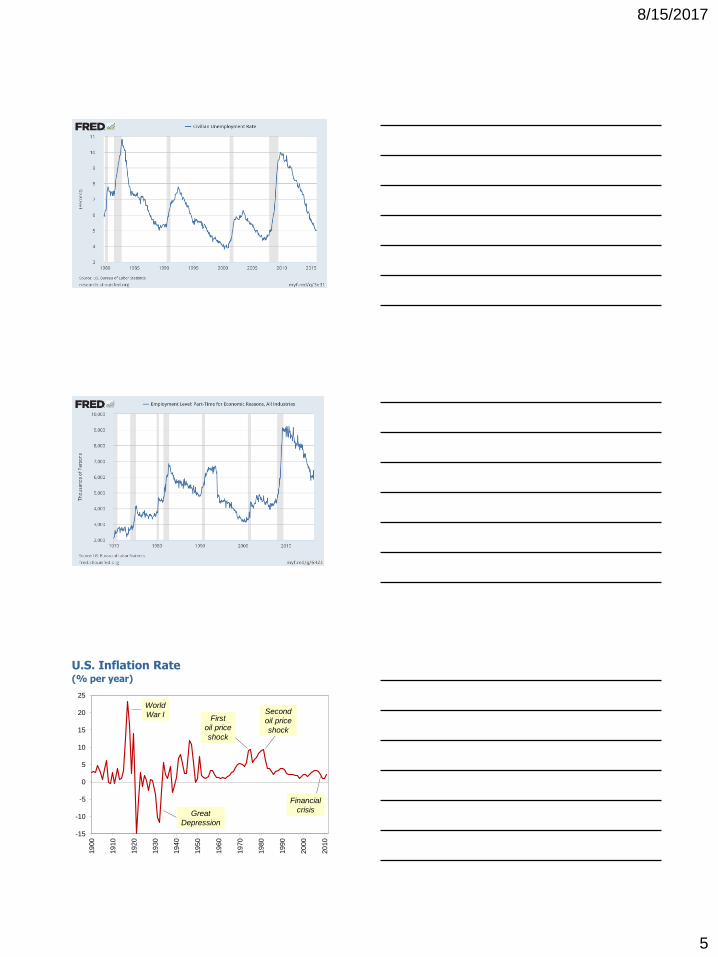
U.S. Unemployment Rate

(% of labor force)

Great

Depression

First

oil price

shock

Second

oil price

shock

Financial

crisis

World

War I

0

5

10

15

20

25

30

19

00

19

10

19

20

19

30

19

40

19

50

19

60

19

70

19

80

19

90

20

00

20

10

Great

Depression

Financial

crisis World

War II

World

War I Oil price

shocks

8/15/2017

5

U.S. Inflation Rate (% per year)

-15

-10

-5

0

5

10

15

20

25

19

00

19

10

19

20

19

30

19

40

19

50

19

60

19

70

19

80

19

90

20

00

20

10

Great

Depression

First

oil price

shock

Second

oil price

shock

Financial

crisis

World

War I

8/15/2017

6

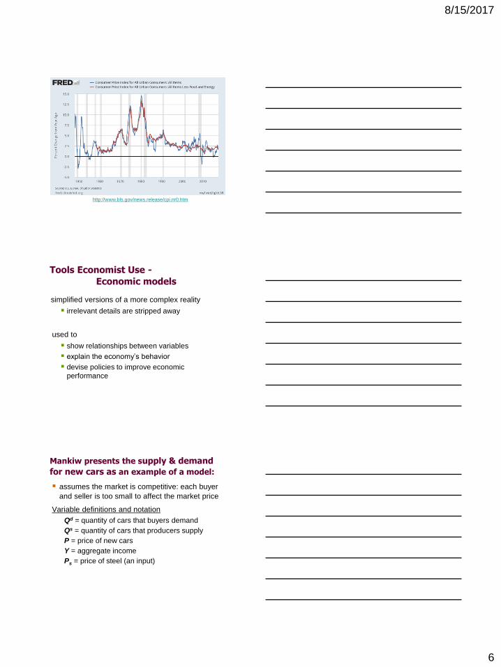
http://www.bls.gov/news.release/cpi.nr0.htm

Tools Economist Use -

Economic models

simplified versions of a more complex reality

irrelevant details are stripped away

used to

show relationships between variables

explain the economy’s behavior

devise policies to improve economic

performance

Mankiw presents the supply & demand

for new cars as an example of a model:

assumes the market is competitive: each buyer

and seller is too small to affect the market price

Variable definitions and notation

Qd = quantity of cars that buyers demand

Qs = quantity of cars that producers supply

P = price of new cars

Y = aggregate income

Ps = price of steel (an input)

8/15/2017

7

The demand for cars:

demand equation: Q d = D (P,Y )

Read as quantity demanded is a function of

(depends upon) the price of new cars (P) and

aggregate income (Y).

Shows that the quantity of cars consumers

demand is related to the price of cars and

aggregate income

Digression: functional notation

General functional notation

shows only that the variables are related.

Q d = D (P,Y )

A specific functional form shows the precise

quantitative relationship.

Example:

Q d =D (P,Y ) = 60 – 10P + 2Y

The market for cars: Demand

Q

Quantity of cars

P Price

of cars

D

The demand curve

shows the relationship

between quantity

demanded and price,

other things equal.

demand equation:

Q d = D (P,Y )

8/15/2017

8

The market for cars: Supply

Q

Quantity of cars

P Price

of cars

D

S

The supply curve

shows the relationship

between quantity

supplied and price,

other things equal.

supply equation:

Q s = S (P,PS )

The market for cars: Equilibrium

Q

Quantity of cars

P Price

of cars S

D

equilibrium

price

equilibrium

quantity

The effects of an increase in income

Q

Quantity of cars

P Price

of cars S

D1

Q1

P1

An increase in income

increases the quantity

of cars consumers

demand at each price…

…which increases

the equilibrium price

and quantity.

P2

Q2

D2

demand equation:

Q d = D (P,Y )

8/15/2017

9

The effects of a steel price increase

Q

Quantity of cars

P Price

of cars S1

D

Q1

P1

An increase in Ps

reduces the quantity of

cars producers supply

at each price…

…which increases the

market price and

reduces the quantity.

P2

Q2

S2

supply equation:

Q s = S (P,PS )

Endogenous vs. exogenous variables

The values of endogenous variables

are determined in the model.

The values of exogenous variables

are determined outside the model:

the model takes their values & behavior

as given.

In the model of supply & demand for cars,

endogenous: P, Qd, Qs

exogenous: Y, Ps

NOW YOU TRY:

Supply and Demand

1. Market for Pizza

2.

3.

4. Solve for equilibrium P and Q

60 10 2dQ P Y

100 5 15sQ P Pc

8/15/2017

10

The use of multiple models

No one model can address all the issues we

care about.

E.g., our supply-demand model of the car

market…

can tell us how a decrease in aggregate income

affects price & quantity of cars.

cannot tell us why aggregate income falls.

The use of multiple models

So we will learn different models for studying

different issues (e.g., unemployment,

inflation, long-run growth).

For each new model, you should keep track of

its assumptions

which variables are endogenous,

which are exogenous

the questions it can help us understand,

those it cannot

Prices: flexible vs. sticky

Market clearing: An assumption that prices are

flexible, adjust to equate supply and demand.

In the short run, many prices are sticky –

adjust sluggishly in response to changes in

supply or demand. For example:

many labor contracts fix the nominal wage

for a year or longer

many magazine publishers change prices

only once every 3-4 years

8/15/2017

11

Prices: flexible vs. sticky

The economy’s behavior depends partly on

whether prices are sticky or flexible:

If prices sticky (short run),

demand may not equal supply, which explains:

unemployment (excess supply of labor)

why firms cannot always sell all the goods

they produce

If prices flexible (long run), markets clear and

economy behaves very differently

Outline of the book:

Introductory material (Chaps. 1, 2)

Classical Theory (Chaps. 3–7)

How the economy works in the long run, when

prices are flexible

Growth Theory (Chaps. 8, 9)[Not covered]

The standard of living and its growth rate over the

very long run

Business Cycle Theory (Chaps. 10–14)

How the economy works in the short run, when

prices are sticky

Outline of the book:

Macroeconomic theory (Chaps. 15–17)

Macroeconomic dynamics, models of consumer

behavior, theories of firms’ investment decisions

Macroeconomic policy (Chaps. 18–20)

Stabilization policy, government debt and

deficits, financial crises

8/15/2017

12

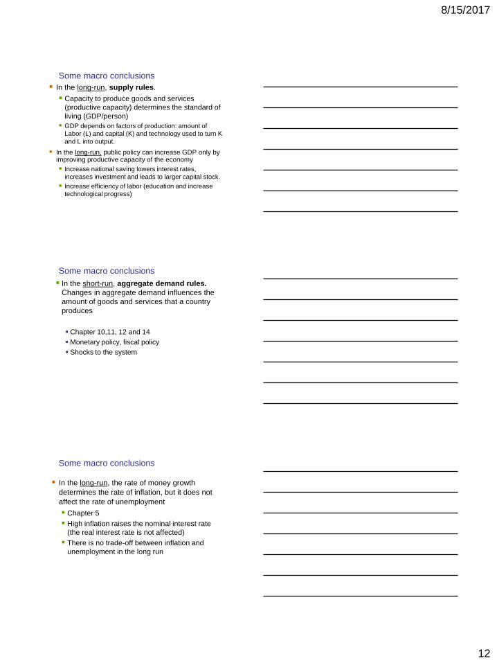
In the long-run, supply rules.

Capacity to produce goods and services

(productive capacity) determines the standard of

living (GDP/person)

GDP depends on factors of production: amount of

Labor (L) and capital (K) and technology used to turn K

and L into output.

In the long-run, public policy can increase GDP only by improving productive capacity of the economy

Increase national saving lowers interest rates,

increases investment and leads to larger capital stock.

Increase efficiency of labor (education and increase

technological progress)

Some macro conclusions

In the short-run, aggregate demand rules.

Changes in aggregate demand influences the

amount of goods and services that a country

produces

Chapter 10,11, 12 and 14

Monetary policy, fiscal policy

Shocks to the system

Some macro conclusions

In the long-run, the rate of money growth

determines the rate of inflation, but it does not

affect the rate of unemployment

Chapter 5

High inflation raises the nominal interest rate

(the real interest rate is not affected)

There is no trade-off between inflation and

unemployment in the long run

Some macro conclusions

8/15/2017

13

There is a trade-off between inflation and

unemployment in the short-run

Chapter 14, short-run Phillips curve

Increase Aggregate Demand => U↓ and π↑

Contract Aggregate Demand => U↑ and π↓

Some macro conclusions