Managing water resources system in a mixed inexact environment using superiority and inferiority measures

ORIGINAL PAPER

Managing water resources system in a mixed inexact environmentusing superiority and inferiority measures

Y. Lv • G. H. Huang • Y. P. Li • W. Sun

Published online: 2 November 2011

� Springer-Verlag 2011

Abstract A superiority–inferiority-based fuzzy-stochas-

tic integer programming (SI-FSIP) method is developed for

water resources management under uncertainty. In the SI-

FSIP method, techniques of fuzzy mathematical program-

ming with the superiority and inferiority measures and joint

chance-constrained programming are integrated into an

inexact mixed integer linear programming framework. The

SI-FSIP improves upon conventional inexact fuzzy pro-

gramming by directly reflecting the relationships among

fuzzy coefficients in both the objective function and con-

straints with a high computational efficiency, and by

comprehensively examining the risk of violating joint

probabilistic constraints. The developed method is applied

to a case study of water resources planning and flood

control within a multi-stream and multi-reservoir context,

where several studied cases (including policy scenarios)

associated with different joint and individual probabilities

are investigated. Reasonable solutions including binary and

continuous decision variables are generated for identifying

optimal strategies for water allocation, flood diversion and

capacity expansion; the tradeoffs between total benefit and

system-disruption risk are also analyzed. As the first

attempt for planning such a water-resources system through

the SI-FSIP method, it has potential to be applied to many

other environmental management problems.

List of symbols

A01;A

02

Storage area coefficients for Reservoirs 1

and 2, respectively

A1a, A2

a Areas per unit of active storage volume

above A10 and A2

0, respectively

CFD Upper limit of flood diversion (m3)

DAimax, DBi

max Maximum water amounts that can be

allocated to user i for Cities A and B,

respectively (m3)

e1±, e2

± Mean evaporation rates of Reservoirs 1

and 2, respectively (m)

EC± Cost for expanding capacity of flood

diversion ($)

f± Objective function value, expected net

system benefit ($)

FC± Fixed-charge cost for flooding diversion

($)

ia, ib Water users in Cities A and B, ia ¼ 1; 2;

. . .; Ia and ib ¼ 1; 2; . . .; Ib; respectively

k1, k2 Possible scenarios for flows of Streams

1 and 2; k1 ¼ 1; 2; . . .;K1

and k2 ¼ 1; 2; . . .;K2; respectively

NBA1±, NBB1

± Net benefit to user i of Cities A and B per

unit of water allocated ($/m3)

pk1; pk2

Probabilities of occurrences for scenarios

k1 and k2, respectively

Q�k1; Q�k2

Random inflows into Streams 1 and 2

under scenarios k1, k2, respectively (m3)

Y. Lv � G. H. Huang (&) � Y. P. Li

MOE Key Laboratory of Regional Energy Systems

Optimization, S&C Academy of Energy and Environmental

Research, North China Electric Power University, Beijing

102206, China

e-mail: [email protected]

Y. Lv


Y. P. Li


W. Sun

Faculty of Engineering and Applied Science, University of

Regina, Regina, SK S4S0A2, Canada


123

Stoch Environ Res Risk Assess (2012) 26:681–693

DOI 10.1007/s00477-011-0533-1

R�k1Release flow from Reservoir 1 associated

with probability of Pk1(m3)

R�k1k2Release flow from Reservoir 2 associated

with probability of pk1� pk2

(m3)

RD± Downstream water level (m3)

RSC1±, RSC2

± Storage capacities of Reservoirs 1 and 2,

respectively (m3)

RSV1±, RSV2

± Reserved storage volumes for Reservoirs

1 and 2, respectively (m3)

S�k1Storage level in Reservoir 1 under

scenarios k1 (m3)

S�k1k2Storage level in Reservoir 2 under

scenarios k1 and k2 (m3)

SI1±, SI2

± Initial storage volumes in Reservoirs 1

and 2, respectively (m3)~Tmax

a ; ~Tmaxb

Maximum water resources amounts that can

be allocated to Cities A and B, respectively

(m3)

VC� Variable cost for flooding diversion ($/m3)

XCAi±, XCBi

± Decision variables, water amounts

allocated to users in Cities A and B(m3)

XT�k1k2Surplus-flow to be diverted under

scenarios k1 and k2 (m3)

Yk1k2Binary variable identifying whether or

not a flood-diversion action needs to be

undertaken under scenarios k1 and k2

Z Binary variable identifying whether or

not the capacity of floodplain needs to be

expanded

b Joint probability of violating constraints of

the reservoir-storage capacities (b [ [0, 1])

1 Introduction

Water allocation among municipal, industrial and agricul-

tural users is vital to water resources management. The

disparate groups of water users need to know how much

water they can expect in order to make appropriate deci-

sions regarding their various activities and investments

(Guo et al. 2010b). Optimal use of available water

resources can result in efficient utilization to maximize the

benefits (Khare and Jat 2006; Obeysekera et al. 2011; Si-

vakumar 2011). However, such planning efforts in real-

world cases are often complicated by a number of highly

uncertain parameters and their interrelationships, as well as

interactions between the uncertain parameters and the

associated economic implications. For example, spatial and

temporal variations may cause uncertainties to exist in

system components, such as stream flows and water allo-

cation patterns, as well as benefits from water utilizations

and costs for flood diversion and floodplain capacity

expansion. These difficulties place the planning problem

beyond the conventional programming methods. Therefore,

there is an urgent need to develop innovative approaches

for efficient, equitable and sustainable water-resources

management under uncertainties.

Previously, there were many optimization methods for

assisting in the formulation of water resources management

plans generally based on interval, fuzzy, and stochastic

programming approaches (Huang 1996; Colby et al. 2000;

Despic and Simonovic 2000; Watkins et al. 2000; 2002;

Akter and Simonovic 2005; Chang 2005; Lee and Chang

2005; Maqsood et al. 2005; Fu 2008; Li et al. 2009; Liu and

Huang 2009; Zarghami and Szidarovszky 2009; Guo et al.

2010a; Li and Huang 2010b; Zhou and Huang 2011). For

example, Huang (1996) proposed an interval-parameter

programming (IPP) method for dealing with uncertainties

expressed as interval numbers in an agricultural water

resources management system. Fu (2008) presented an

optimization method for reservoir flood control operation,

which was based on the concept of ideal and anti-ideal

points to solve multi-criteria decision making problems

under fuzzy environments. Liu and Huang (2009) proposed

a dual interval two-stage programming for water resources

planning, where the system risk could be reflected through

the restricted-resource measure by controlling the vari-

ability of the recourse cost. Among the above optimization

approaches, fuzzy mathematical programming (FMP) was

capable of handling uncertainties presented as fuzzy sets,

and was effective in reflecting ambiguity and vagueness in

resource availabilities that present on the right-hand sides

of the model (Inuiguchi et al. 1990). To solve the FMP

problems, various approaches were proposed through uti-

lizing ranking operations (e.g., the area compensation and

signed distance methods) and discretizing fuzzy sets via a-

cuts (e.g., robust programming) (Fortemps and Roubens

1996; Inuiguchi and Sakawa 1998; Tan et al. 2010a).

However, these methods could generate a large number of

additional constraints and variables, and thus result in

complicated and time-consuming computation processes

(Van Hop 2007). Van Hop (2007) proposed a superiority–

inferiority-based fuzzy linear programming (SI-FSLP)

method to tackle these difficulties. The SI-FSLP could

directly reflect relationships among fuzzy parameters

through varying superiority and inferiority degrees, where

the implement of stochastic programming techniques after

the defuzzification process was not required any more.

Through quantifying economic penalties of potential con-

straint violations, the original models then could be trans-

formed into equivalent deterministic ones. Thus, the SI-

FSLP method can lead to a sharp decline in computational

efforts and be easily solved compared with the conven-

tional FMP methods. Tan et al. 2010b successfully used the

superiority and inferiority measures to address fuzziness in

682 Stoch Environ Res Risk Assess (2012) 26:681–693

123

the municipal solid waste management systems; however,

this method had difficulties in tackling uncertainties

expressed as probability distributions; in particular, when

the probability level is restricted to a set of constraints as a

whole. Joint chance-constrained programming (JCP) could

effectively reflect the reliability of satisfying (or risk of

violating) system constraints under joint probability

uncertainties. The JCP requires the whole set of uncertain

constraints are enforced to be satisfied at least at a proba-

bility level; this allows an increased robustness in con-

trolling system risk in the optimization process (Zhang

et al. 2002; Lejeune and Prekopa 2005; An and Eheart

2007). Few research efforts focused on JCP’s application to

planning water resources management systems (Li et al.

2009; Li and Huang 2010a; Lv et al. 2011).Therefore, one

potential approach for better accounting for the complex-

ities and uncertainties of water resources management and

planning is to link the FMP with the JCP.

On the other hand, for water resources management

problems, people may face the potential threats caused by

flooding in the case of sufficient water. In the past decades,

frequently occurring floods claimed thousands of lives and

resulted in tremendous economic losses (Huang 2005). In

the United States, flooding killed more than 10,000 people

during the twentieth century and the relevant property

damage totaled more than US $1 billion per year (FEMA

2002). Inexact mixed-integer linear programming (IMIP)

can be used to help make decisions on whether or not

particular actions (e.g., flood diversion and floodplains

expansion) are to be undertaken under uncertainty (Wind-

sor 1981; Randall et al. 1997; Srinivasan et al. 1999;

Needham et al. 2000; Olsen et al. 2000; Li et al. 2010). In

IMIP, uncertain parameters expressed as interval numbers

(with known lower and upper bounds but unknown mem-

bership functions or probability distributions) can be

directly communicated into the optimization process and

resulting solutions, such that multiple decision alternatives

can be generated through the interpretation of the solutions

(Huang et al. 1995b; Lv et al. 2009).

Therefore, the objective of this study is to develop a

superiority–inferiority-based fuzzy-stochastic integer pro-

gramming (SI-FSIP) method for planning of water

resources management system. In the SI-FSIP method,

techniques of fuzzy mathematical programming (FMP)

with the superiority and inferiority measures and joint

chance-constrained programming (JCP) will be integrated

into an inexact mixed integer linear programming (IMIP)

framework. The SI-FSIP will be able to deal with uncer-

tainties expressed as fuzzy sets, probability distributions

and interval values. A case study will then be provided to

demonstrate how the developed method with a high com-

putational efficiency can (a) support the planning for water

resources management with a multi-stream, multi-reservoir

context under joint-probabilistic constraints, and (b) help

identify desired plans of water allocation and flood diver-

sion with a maximized system benefit and a minimized

constraint-violation risk.

2 Methodology

2.1 Development of SI-FSIP model

An inexact mixed-integer linear programming (IMIP)

model incorporating the technique of interval-parameter

programming (IPP) within a mixed integer linear pro-

gramming (MIP) framework can tackle uncertainties pre-

sented as discrete intervals and to facilitate dynamic

analyses of capacity-expansion decisions (Huang et al.

1995a). In detail, an IMIP problem can be formulated as:

Max f� ¼ C�X� ð1aÞ

subject to:

A�X� � B� ð1bÞ

X� � 0 ð1cÞ

where A� 2 R�� m�n

; B� 2 R�� m�1

; C� 2 R�� 1�n

;

X� 2 R�� n�1

and R� denotes a set of interval values. In

model (1), decision variables (X±) can be divided into two

categories: continuous and binary. Apparently, IMIP can

hardly tackle uncertainties expressed as fuzzy sets and

probabilistic distributions.

In order to deal with uncertain parameters presented as

interval values and fuzzy sets, an inexact fuzzy integer

programming (IFIP) method is provided as follows:


subject to:

A�X� � B� ð2bÞ~G�X� � ~w ð2cÞ

X� � 0 ð2dÞ

where ~G� and ~w can be presented as fuzzy sets.

Then, the superiority and inferiority measures can be

introduced to solve the above problem via a more efficient

way, such that a superiority–inferiority-based IFIP model

can be formulated. According to Zimmermann 1991 and

Van Hop (2007), let ~H be a family of triangular fuzzy

numbers which can be defined as follows:

~H ¼ ~d ¼ d; a; bð Þ; a; b � 0n o

ð3aÞ

Stoch Environ Res Risk Assess (2012) 26:681–693 683

123

l�dðxÞ ¼max 0; 1� d�x

a

� �if x � d; a [ 0

1 if a ¼ 0 and=or b ¼ 0

max 0; 1� d�xb

� �if x [ d; b [ 0

0 otherwise

8>><

>>:ð3bÞ

where scalars a and b (a, b C 0; a, b [ R) are named the

left and right spreads, respectively. ~d is a crisp number

~d 2 R� �

that can be illustrated as a triangular fuzzy set

~d ¼ d; 0; 0ð Þ:Based on the above definitions, a method for compar-

ing fuzzy sets can be proposed through measuring supe-

riority and inferiority degrees. Two fuzzy sets associated

with a-cut levels can be defined as follows (Van Hop

2007):

~Pa ¼ lP� xð Þ � a ð4aÞ~Qa ¼ lQ� xð Þ � a ð4bÞ

If ~Pa � ~Qa, then sup s : lQ� sð Þ � a� �

� sup t : lP�ftð Þ � ag. Therefore, the total superiority of ~Q over ~P is

defined as the area of ~Q larger than ~P. Mathematically, this

area can be presented as follows:

S¼

R 1

0sup s : lQ� sð Þ � a� ��

� sup t : lP� tð Þ � af ggda � 0 if ~Q � ~P

0 otherwise

8><

>:ð5aÞ

Similar result can also be obtained for the inferior

degree of ~P to ~Q:

I ¼

R 1

0inf s : lQ� sð Þ � a� ��

� inf t : lP� tð Þ � af ggda � 0 if ~Q � ~P

0 otherwise

8><

>:ð5bÞ

Thus, the superiority of ~Q over ~P can be defined as

S ~Q; ~P� �

¼Z1

0

max 0; sup s : lQ� sð Þ � a� ��

� sup t : lP� tð Þ � af ggda � 0

ð6aÞ

Analogously, the inferiority of ~P to ~Q is

I ~Q; ~P� �

¼Z1

0

max 0; inf s : lQ� sð Þ � a� ��

� inf t : lP� tð Þ � af ggda � 0

ð6bÞ

Considering two triangular fuzzy sets ~P ¼ p; tpl; tpr

� �;

~Q ¼ q; tql; tqr

� �; and ~P; ~Q 2 ~H (Fig. 1), the superiority of ~Q

over ~P and the inferiority of ~P to ~Q thus can be defined as

follows (Van Hop 2007):Superiority S ~Q; ~P� �

S ~Q; ~P� �

¼ q� pþ tqr � tpr

2ð7Þ

Inferiority I ~P; ~Q� �

I ~P; ~Q� �

¼ q� pþ tql � tpl

2ð8Þ

Moreover, when the requirement of satisfactory level is

imposed on a set of constraints as a whole, the randomness

in the right-hand sides of the constraints needs to be

tackled. Thus, the joint chance-constrained programming

(JCP) can be introduced to deal with the above

uncertainties. Generally, a linear JCP model can be

expressed as follows (Miller and Wagner 1965; Lejeune

and Prekopa 2005; Lv et al. 2011):

Max cT x ð9aÞ

subject to:

Trx � F�1r brð Þ; r ¼ 1; 2; . . .;R ð9bÞ

XR

r¼1

br � b ð9cÞ

Ax � b ð9dÞx � 0 ð9eÞ

where A is an [m 9 n]-dimensional matrix; Tr is an

[r 9 n]-dimensional matrix; c and x are n-dimensional

vectors; b is an m-dimensional vector. brðr ¼ 1; 2; . . .;RÞare individual violating probabilities, 0\br � 1; F�1

r refer

to inverse probability distribution functions of the random

variables (er). When the random variables of model’s right-

hand sides are independent of each another, 1� br are

constrained to be larger than or equal to 1 - b.

Consequently, the JCP can be incorporated within the

above inexact fuzzy integer programming (IFIP) frame-

work, so that uncertainties presented as intervals, fuzzy sets

and joint probabilities can be tackled. The formulated

superiority–inferiority-based fuzzy-stochastic integer pro-

gramming (SI-FSIP) model can be generally expressed as

follows:

Fig. 1 Superiority and inferiority between ~P and Q_


123


subject to:

A�X� � B� ð10bÞ~G�X� � ~w ð10cÞ

Trx � F�1r brð Þ; r ¼ 1; 2; . . .;R ð10dÞ

XR

r¼1

br � b ð10eÞ

X� � 0 ð10fÞ

2.2 Solution method

The SI-FSIP model can be transformed into two deter-

ministic sub-models that corresponding to the lower and

upper bounds of the desired objective. Then, the interval

solution can be obtained through solving the two sub-

models sequentially, where the superiorities and inferiori-

ties of fuzzy variables are measured (Huang et al. 1995b;

Van Hop 2007; Lv et al. 2010). Since the SI-FSIP method

is to maximize its objective, the sub-model corresponding

to the upper bound objective (f?) can be firstly formulated

as follows:

Max fþ ¼Xk1

j¼1

cþj xþj þXn1

j¼k1þ1

cþj x�j ð11aÞ

subject to:

Xk1

j¼1

aij j�Sign a�i� �

xþj þXn1

j¼k1þ1

aij jþSign aþi� �

x�j � bþi ; 8i

ð11bÞ

Xk1

j¼1

~gvj j�Sign ~g�v� �

xþj þXn1

j¼k1þ1

~gvj jþSign ~gþv� �

x�j � ~w; 8v

ð11cÞ

Trxþ � F�1

r brð Þ; r ¼ 1; 2; . . .;R ð11dÞ

XR

r¼1

br � b ð11eÞ

xþj � 0; j ¼ 1; 2; . . .; k1 ð11fÞ

x�j � 0; j ¼ k1 þ 1; k1 þ 2; . . .; n1 ð11gÞ

Model (11) requires a maximized objective function value

subject to a superiority of the right-hand sides (RHS) over the

left-hand sides (LHS) and an inferiority of LHS to RHS.

Based on the concepts of the superiority and inferiority, the

above problem can be reformulated by paying a penalty to

any violation caused by variations in fuzziness; this

corresponds to a maximized objective function value

subject to penalty costs for violating superiority of RHS

over LHS and inferiority of LHS to RHS. Then, model (11)

can be re-formulated as follows:

Max fþ ¼Xk1

j¼1

cþj xþj þXn1

j¼k1þ1

cþj x�j � ds

X

v

Sv

Xk1

j¼1


xþj þXn1

j¼k1þ1


x�j ; ~w

!

� dI

X

v

Iv ~w;Xk1

j¼1


xþj

þXn1

j¼k1þ1


x�j

!

ð12aÞ

subject to:

Xk1

j¼1

aij j�Sign a�i� �

xþj þXn1

j¼k1þ1

aij jþSign aþi� �

x�j � bþi ; 8i

ð12bÞ

Trxþ � F�1

r brð Þ; r ¼ 1; 2; . . .;R ð12cÞ

XR

r¼1

br � b ð12dÞ

xþj � 0; j ¼ 1; 2; . . .; k1 ð12eÞ

x�j � 0; j ¼ k1 þ 1; k1 þ 2; . . .; n1 ð12fÞ

where dS and dI are penalty coefficients, and dS [ 0, dI [0.

Consequently, solutions of xþj opt j ¼ 1; 2; . . .; k1ð Þ and x�j opt

j ¼ k1 þ 1; k1 þ 2; . . .; n1ð Þ can be obtained through sub-

model (12). Similarly, the sub-model corresponding to f- can

be formulated accordingly, where solutions of xþj opt j ¼ð1; 2; . . .; k1Þ and x�j opt j ¼ k1 þ 1; k1 þ 2; . . .; n1ð Þ can be

obtained. Therefore, the general solutions are provided as

follows:

x�j opt ¼ x�j opt; xþj opt

h i; 8j ð13Þ

f�opt ¼ f�opt; fþopt

h ið14Þ

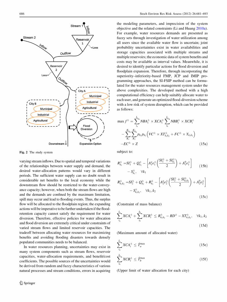
3 Case study

In the study region (Fig. 2), two streams and two reservoirs

can supply water to two cities (i.e., A and B), with a floodplain

region designed for flood diversion. To meet demands for

regional socio-economic development, the local authority is

responsible for water allocation to municipal, industrial and

agricultural sectors as well as for flood control and environ-

mental protection in the cities. The authority needs to know

how much water can be optimally allocated to each user under


123

varying stream inflows. Due to spatial and temporal variations

of the relationships between water supply and demand, the

desired water-allocation patterns would vary in different

periods. The sufficient water supply can no doubt result in

considerable net benefits to the local economy while the

downstream flow should be restricted to the water-convey-

ance capacity; however, when both the stream flows are high

and the demands are confined by the maximum limitation,

spill may occur and lead to flooding events. Thus, the surplus

flow will be allocated to the floodplain region; the expanding

actions will be imperative to be further undertaken if the flood-

retention capacity cannot satisfy the requirement for water

diversion. Therefore, effective policies for water allocation

and flood diversion are extremely critical under constraints of

varied stream flows and limited reservoir capacities. The

tradeoff between allocating water resources for maximizing

benefits and avoiding flooding disasters towards densely

populated communities needs to be balanced.

In water resources planning, uncertainties may exist in

many system components such as stream flows, reservoir

capacities, water-allocation requirements, and benefit/cost

coefficients. The possible sources of the uncertainties would

be derived from random and fuzzy characteristics of various

natural processes and stream conditions, errors in acquiring

the modeling parameters, and imprecision of the system

objective and the related constraints (Li and Huang 2010a).

For example, water resources demands are presented as

fuzzy sets through investigation of water utilization among

all users since the available water flow is uncertain; joint

probability uncertainties exist in water availabilities and

storage capacities associated with multiple streams and

multiple reservoirs; the economic data of system benefits and

costs may be available as interval values. Meanwhile, it is

desired to identify particular actions for flood diversion and

floodplain expansion. Therefore, through incorporating the

superiority–inferiority-based FMP, JCP and IMIP pro-

gramming approaches, the SI-FSIP method can be formu-

lated for the water resources management system under the

above complexities. The developed method with a high

computational efficiency can help suitably allocate water to

each user, and generate an optimized flood-diversion scheme

with a low risk of system disruption, which can be provided

as follows:

max f� ¼XIa

ia

NBA�i � XCA�iXIa

ib

NBB�i � XCB�i

�XK1

K1

XK2

K2

pk1pk2

VC� � XT�k1k2þ FC� � Yk1k2

� �

�EC� � Z ð15aÞ

subject to:

R�k1¼SI�1 þ Q�k1

� Aa1e�1

SI�1 þ SI�k1

2

� þ A0

1e�1

�

� S�k1; 8k1

ð15bÞ

R�k1k2¼SI�2 þ Q�k2

þ R�k1� Aa

2e�2SI�2 þ SI�k1k2

2

� þ A0

2e�2

�

� S�k1k2; 8k1; k2

ð15cÞ

(Constraint of mass balance)

XIa

ia

XCA�i þXIb

ib

XCB�i � R�k1k2� RD� � XT�k1k2

; 8k1; k2

ð15dÞ

(Maximum amount of allocated water)

XIa

ia

XCA�i � ~Tmaxa ð15eÞ

XIb

ib

XCB�i � ~Tmaxb ð15fÞ

(Upper limit of water allocation for each city)

Fig. 2 The study system


123

PrS�k1� RSC1; 8k1

S�k1k2� RSC2; 8k1k2

� � 1� b ð15gÞ

(Joint-probabilistic constraint for storage capacities of

reservoirs)

S�k1� RSV�1 ; 8k1 ð15hÞ

S�k1k2� RSV�2 ; 8k1; k2 ð15iÞ

(Requirement for minimum storage)

Yk1k2¼ 1; if XT�k1k2

[ 0

0; if XT�k1k2¼ 0

; 8k1; k2

�ð15jÞ

(Identification of flood-diversion action)

Z ¼ 1; if XT�k1k2[ CFD

0; if XT�k1k2� CFD

; 8k1; k2

�ð15kÞ

(Identification of capacity-expansion action)

0 � XCA�i � DAmaxi ; 8i ð15lÞ

0 � XCB�i � DBmaxi ; 8i ð15mÞ

(Water allocation required by each user)

XT�k1;k2� 0; 8k1; k2 ð15nÞ

(Constraint of non-negative variable)

The detailed nomenclatures for the variables and

parameters are provided in the Appendix. The decision

variables of model (15) can be sorted into two categories:

continuous and binary. The continuous variables XCA�i ;�

XCB�i and XT�k1k2Þ represent water resources amounts for

allocation and diversion. The binary variables Yk1k2and Zð Þ

indicate whether or not flood-diversion and floodplains-

expansion actions need to be carried out over the planning

horizon. In the system, the normally distributed inflows of

the two streams are presented as discrete random variables

associated with probabilities of occurrences (Table 1).

Moderate water allocations can bring net benefits for the

cities; higher stream inflows may lead to a raised surplus

that needs to be diverted effectively. Table 2 provides the

economic information of water allocation and flood

diversion. In addition, the random storage capacities of

Reservoirs 1 and 2 are 39.0 9 106 m3 (r = 3.90 9 106)

and 44.5 9 106 m3 (r = 4.45 9 106), respectively; the

initial storages in Reservoirs 1 and 2 are [16.2, 18.0] 9

106 m3 and [24.6, 27.3] 9 106 m3, respectively; the

reserved storage levels for Reservoirs 1 and 2 are [10.6,

11.7] 9 106 m3 and [13.5, 14.9] 9 106 m3, respectively;

the maximum water resources amounts allocated to Cities

A and B are specified as triangle fuzzy numbers of (37.0, 5,

5) 9 106 m3 and (45.0, 5, 5) 9 106 m3, respectively.

4 Result analysis

In this study, a set of chance constraints for the storage

capacities of the two reservoirs are considered, which can

help investigate the risk of violating the capacity con-

straints and generate desired water-allocation and surplus-

flow diversion schemes. Nine cases (Table 3) are examined

corresponding to various policies for water resources

management and multiple joint probabilities associated

with different sets of discrete individual probabilities. For

instance, Case 1–1 denotes that when the allowable vio-

lating probability (joint probability) of reservoir capacities

is 0.05, the individual probabilities are 0.025 for Reservoir

1 and 0.025 for Reservoir 2, respectively. Figure 3 shows

the solutions of water-allocation patterns and the associated

benefits, which are generated in Case 1–1 (b = 0.05) for

municipal, industrial and agricultural sectors in Cities A

and B, respectively. In detail, in city A, the optimized

water allocation amounts would be 17.5 9 106 m3 for

municipal sector, 12.5 9 106 m3 for industrial sector, and

9.5 9 106 m3 for agricultural sector, respectively. In city

B, the water amounts allocated to the three sectors would

be 22.0 9 106, 15.8 9 106 and 9.7 9 106 m3, respectively.

Meanwhile, benefits can be obtained from the utilizations

of water resources by these sectors in Cities A and B.

Among the three sectors, the municipality could bring the

highest benefits due to the maximum allocation amounts

and the highest net benefits per unit of water. Benefits

derived from municipal sectors in Cities A and B are

$[605.5, 743.8] 9 106 and $ [838.2, 1029.6] 9 106,

respectively. In comparison, industry and agriculture cor-

respond to lower benefits, which are $[317.5, 380.0] 9 106

and $[136.8, 169.1] 9 106 in city A, and $[440.8,

527.7] 9 106 and $ [153.3, 190.1] 9 106 in city B,

respectively.

Due to the temporal and spatial variations of both stream

inflows and water availability, surplus would occur in most

of flow scenarios (except L–L, L–M and LM–L in Case 1–1)

so that flood-diversion schemes would be made to avoid

spill accordingly. Since there are respectively five and

Table 1 Stream inflows at different probabilities (106 m3)

Inflow level Probability Stream Inflow

(106 m3)

Stream 1 Low (L) 0.12 [72.5, 80.5]

Low-Medium (L–M) 0.21 [80.3, 89.2]

Medium (M) 0.34 [98.5, 109.4]

Medium–High (M–H) 0.23 [116.5, 129.4]

High (H) 0.10 [167.7, 186.3]

Stream 2 Low (L) 0.24 [31.8, 35.3]

Medium (M) 0.49 [41.8, 46.4]

High (H) 0.27 [59.0, 65.5]


123

three flow levels for Streams 1 and 2, a total of 15 flow

scenarios are generated. The diverted water amounts may

vary at different flow levels (Table 4). When the inflows of

stream 1 and 2 are both high (denoted as scenario H–H),

the amount for flood diversion would be 116.91 9 106 m3

at a probability level of 2.70%. Moreover, the result of the

binary variable Z indicates that the diverted water amount

under this scenario cannot be satisfied by the capacity of

floodplain (115.00 9 106 m3). Thus, the capacity-expan-

sion action for the floodplain would be undertaken to

prevent flood disasters and to increase the diversion

allowances within the system. In Case 1–1, the system

would be expanded by an increment of 1.16 9 106 m3

under the inflow scenario of H–H in response to the local

flood control policy. Consequently, the total net benefit

would be the benefits from water allocations minus the

costs from both flood diversion and capacity expansion

($[1241.2, 1904.2] 9 106). The interval objective function

value is associated with two bounds of benefit and cost

coefficients, where upper bounds of benefits and lower

bounds of costs correspond to higher system benefit (f?),

and vice versa.

In the case of flood events, the water-diversion schemes

would be different from each other at varied joint- and

individual-probability levels. Table 4 also presents the

solutions of the continuous and binary variables for flood

control strategies in Cases 1–1 (b = 0.05), 2 –

1 (b = 0.01) and 3 – 1 (b = 0.10), respectively. Both

Cases 1–1 and 2–1 would obtain twelve non-zero binary

variables of Yk1k2, which means flood-diversion actions

should be undertaken under these flow scenarios (i.e., L–H,

LM–M, LM–H, M–L, M–M, M–H, MH–L, MH–M, MH–

H, H–L, H–M and H–H). In particular, when the flow

levels of Streams 1 and 2 are respectively low-medium and

medium (i.e., scenario LM–M with an occurrence proba-

bility of 10.29%), there would be 0.71 9 106 m3 and

6.16 9 106 m3 water diverted to the floodplain in Cases 1–

1 and 2–1, respectively. Comparatively, under scenario

LM–L in Case 3–1, no surplus flow need to be diverted

anywhere; thus, eleven non-zero binary variables of Yk1k2

could be generated from the studied case. In addition, the

results also indicate that the capacity-expansion project of

floodplain should be under consideration in Cases 1–1 and

2–1 over the planning horizon, so that the excess flows of

1.91 9 106 m3 in Case 1–1 and 7.36 9 106 m3 in Case

2–1 can be diverted as well. Generally, an increased b level

means a raised risk of constraint violation, leading to both

decreased strictness for the reservoirs’ capacities and lower

flood-diversion amounts, and vice versa. Moreover, the

solutions of diverted water amounts would also vary at

individual probability (bi) of each reservoir-capacity con-

straint (equal to the joint probability level, b). Figure 4

provides the optimized water-diversion plans under flow

scenarios of H–L, H–M and H–H. In general, different bi

levels correspond to different available storage capacities,

leading to varied flood-diversion patterns over the planning

horizon.

Figure 5 presents the solutions for system benefits. It is

indicated that any change at joint probabilities of b and the

related individual probability levels (bi) would result in the

variations of total benefits. Among all the study cases, only

the objective function value obtained in Case 3–1 would

Table 2 Economic data for

water allocation and flood

diversion

Water use sector City A City B Flood diversion cost

Municipality [34.6, 42.5] [38.1, 46.8] Fixed cost, FC± ($106) [18.0, 19.80]

Industry [25.4, 30.4] [27.9, 33.4] Variable cost, VC± ($/m3) [36.6, 40.3]

Agriculture [14.4, 17.8] [15.8, 19.6] Expansion cost, EC± ($106) [40.0, 44.0]

Table 3 The studied cases at different joint and individual

probabilities

Case No. Joint probability

for the overall

reservoir-storage

capacity (b)

Individual probability

Reservoir

1 (b1)

Reservoir

2 (b2)

1–1 0.05 0.025 0.025

1–2 0.05 0.010 0.040

1–3 0.05 0.040 0.010

2–1 0.01 0.005 0.005

2–2 0.01 0.001 0.009

2–3 0.01 0.009 0.001

3–1 0.10 0.050 0.050

3–2 0.10 0.010 0.090

3–3 0.10 0.090 0.010

Fig. 3 Water-allocation patterns and the associated benefits in Case

1–1


123

not include the cost for capacity expansion; thus, it would

lead to the maximum system benefit of $[1373.7,

2024.5] 9 106. Except that, Case 3–2 (b = 0.10) would

correspond to the highest upper-bound and lower-bound

system benefits (i.e., $[1286.6, 1945.4] 9 106). Case 2–3

(b = 0.10) would have the lowest system benefit ((i.e.,

$[1010.2, 1694.4] 9 106). Variations in the b level corre-

spond to the decision makers’ preferences regarding the

tradeoff between the system benefit and constraint-viola-

tion risk. A higher joint probability level (e.g., 0.10 in

Cases 3–1, 3–2 and 3–3) would sacrifice the system safety

so that the surplus-flow-diversion cost would be reduced

leading to higher system benefits. Conversely, a lower joint

probability level (e.g., 0.01 in Cases 2–1, 2–2 and 2–3)

would result in lower system benefits at a lower constraint-

violation risk. Moreover, under each joint probability level,

the interval objective function values would vary at indi-

vidual probability of each reservoir-capacity constraint

(Fig. 5). Given different water-availability and storage-

capacity conditions as well as their underlying probability

levels, the expected system benefit would change corre-

spondingly between fopt- and fopt

? .

5 Discussion

In the study, the allowable water amounts allocated to

Cities A and B (i.e., ~Tmaxa and ~Tmax

b ) are specified as fuzzy

numbers with tolerances (i.e., 5 9 106 m3). The solutions

generated through the SI-FSIP method would fluctuate with

the variations of these tolerance values. For example, when~Tmax

a can be specified as (37.0, 6, 6) 9 106 m3 (with the

tolerance values of 6 9 106 m3), the water amount allo-

cated to agriculture in city A would be 10.0 9 106 m3.

When the tolerances of ~Tmaxa are 4 9 106 m3 and

Table 4 Solutions in Cases

1–1, 2–1 and 3–1Scenario Occurrence

probability

(%)

Case 1–1 (b = 0.05) Case 2–1 (b = 0.01) Case 3–1 (b = 0.10)

Binary

variable

Yk1k2ð Þ

Diverted

flood

(106 m3)

Binary

variable

Yk1k2ð Þ

Diverted

flood

(106 m3)

Binary

variable

Yk1k2ð Þ

Diverted

flood

(106 m3)

L–L 2.88 0 0 0 0 0 0

L–M 5.88 0 0 0 0 0 0

L–H 3.24 1 11.11 1 16.56 1 8.38

LM–L 5.04 0 0 0 0 0 0

LM–M 10.29 1 0.71 1 6.16 0 0

LM–H 5.67 1 19.81 1 25.26 1 17.08

M–L 8.16 1 9.81 1 15.26 1 7.08

M–M 6.60 1 20.91 1 26.36 1 18.18

M–H 9.18 1 40.01 1 45.46 1 37.28

MH–L 5.52 1 29.81 1 35.26 1 27.08

MH–M 11.27 1 40.91 1 46.36 1 38.18

MH–H 6.21 1 60.01 1 65.46 1 57.28

H–L 2.40 1 86.71 1 92.16 1 83.98

H–M 4.90 1 97.81 1 103.26 1 95.08

H–H 2.70 1 116.91 1 122.36 1 114.18

Floodplain expansion or not Yes Yes No

86.7

1

97.8

1

116.

91

87.3

0

98.4

0

117.

50

87.6

9

98.7

9

117.

89

75

85

95

105

115

125

H-L H-M H-H

flood

div

ersi

on (

106

m3 ) β = 0.05Case 1-1

Case 1-2Case 1-3

92.1

6

103.

26

122.

36

92.8

6

103.

96

123.

06

93.3

6

104.

46

123.

56

H-L H-M H-H

β = 0.01Case 2-1Case 2-2Case 2-3

83.9

8

95.0

8

114.

18

85.3

9

96.4

9

115.

59

86.0

3

97.1

3

116.

23

H-L H-M H-H

β = 0.10Case 3-1Case 3-2Case 3-3

Fig. 4 Diverted flood amounts at flow levels of H–L, H–M and H–H


123

3 9 106 m3, respectively, the agricultural water amounts

allocated to city A would be 9.0 9 106 m3 and

8.5 9 106 m3 accordingly. For city B, the water allocations

to agriculture under different tolerance levels can be

interpreted in the similar way based on the results shown in

Fig. 6. The water amounts allocated to agriculture for the

two cities would be reduced with the decreased tolerance

values. Moreover, the flood-diversion amounts would also

vary with above changes. In detail, when ~Tmaxa and ~Tmax

b are

specified as (37.0, 6, 6) 9 106 m3 and (45.0, 6,

6) 9 106 m3 with the tolerance value of 6 9 106 m3,

respectively, the diverted flood would then be 85.7 9

106 m3 under scenario H–L, 96.8 9 106 m3 under scenario

H–M and 115.9 9 106 m3 under scenario H–H. Generally,

tolerances of each fuzzy number represent the domains

determined by authorities corresponding to the local water

resources management policies. Lower tolerance level

would lead to less available water resources allocated to

users (e.g., the agricultural sector); consequently, more

surplus flow would be required to be diverted at the same

time. In particular, given no tolerance to the allowable

water amounts, fuzzy numbers could be taken on deter-

ministic values; the SI-FSIP would then be turned into an

inexact stochastic mixed integer programming model. The

agricultural allocation water would be 7.0 9 106 m3 for

city A and 7.2 9 106 m3 for city B. The flood to be

diverted under flow scenarios H–L, H–M and H–H would

be 91.7 9 106 m3, 102.8 9 106 m3 and 121.9 9 106 m3,

respectively.

In the SI-FSIP model, the penalty coefficients (dS and dI)

would be determined by decision makers. The relationship

between the system benefit and the penalty coefficients is

investigated. Assuming that dS and dI be the same, let dS

and dI take several discrete values of 0; 5; 10; 15;

20; . . .; 100. Then, the corresponding system benefits (i.e.,

f- and f?) can be obtained. In detail, the variations of f-

and f? with the varied penalty coefficients are as follows:

When dS = dI = 0 and 5, it would result in the highest f-

(i.e., $1373.0 9 106) and f? (i.e., $2050.0 9 106),

respectively. When 5 \ dS = dI \ 30, the lower-bound

and upper-bound benefits would generally decrease with

the increased penalty coefficients. When dS = dI = 30,

both the lower and upper bounds of system benefit would

reach their lowest values that would be $1241.2 9 106 for

f- and $1904.2 9 106 for f?, respectively. When 30 \dS = dI B 100, the system benefit would not change any

more, and remain the same value as that in the situation of

dS = dI = 30,. The larger value of penalty coefficient

would correspond to stricter policies in terms of constraint

violations. On the basis of the above investigation results, a

value of 50 is specified as the penalty coefficient, leading to

the relatively conservative objective function values (sys-

tem benefit). For real-world practice, decision makers can

identify suitable penalty coefficients (i.e., dS = dI) based

on projected applicable conditions in order to obtain the

optimized water allocation and flood diversion schemes.

When the fuzzy numbers in constraints (13e) and (13f)

i:e:; ~Tmaxa and ~Tmax

b

� �are replaced by the interval numbers

([32.0, 42.0] 9 106 m3 and [40.0, 50.0] 9 106 m3,

respectively), the planning problem can thus be solved

through the inexact stochastic integer programming (ISIP)

model. The water allocation pattern for city A would be

17.5 9 106 m3 to municipality, 12.5 9 106 m3 to industry,

and 10.0 9 106 m3 to agriculture, respectively. The water

Fig. 5 Comparison of system benefits

Fig. 6 The water allocations to agriculture

Fig. 7 Comparisons of diverted water amounts obtained from ISIP

and SI-FSIP methods


123

amounts allocated to the above three sectors in city B

would be 22.0 9 106 m3, 15.8 9 106 m3 and 12.2 9

106 m3, respectively. The surplus flows to be diverted

would be less than those obtained from the superiority–

inferiority-based SI-FSIP method (i.e., Case 1–1) under

every flow scenarios, which are provided in Fig. 7. In

particular, the maximum amount of water diverted would

be 113.9 9 106 m3 (compared with 116.9 9 106 m3 from

Case 1–1) under scenario H–H, which means that the flow

levels of Streams 1 and 2 are both high with an occurrence

probability of 2.70%. Thus, the floodplain with a capacity

of 115.00 9 106 m3 would be sufficient for flood diver-

sion, and there would be no capacity-expansion actions to

be undertaken in such a situation. Consequently, the ISIP

method would correspond to a lower system benefit of

$[1153.4, 2088.1] 9 106 (i.e., $[1241.2, 1904.2] 9 106

from Case 1–1). In general, the ISIP solutions can only

reflect the restrictions of allowable water amounts allocated

to Cities A and B with lower and upper bounds. The ISIP

considers no preference from water resources managers so

that the amounts of diverted water under each scenario

would dramatically decrease. The ISIP is unable to incor-

porate various subjective judgments (fuzzy numbers) from

decision makers (or the planners), leading to the losses of

significant uncertain information. Therefore, the superior-

ity–inferiority-based SI-FSIP improves upon the ISIP by

avoiding oversimplification of fuzzy membership functions

to interval parameters.

Moreover, the SI-FSIP can enhance fuzzy robust pro-

gramming (FRP) in terms of computational efficiency.

Although the FRP can also deal with uncertainties in both

left- and right-hand side coefficients as well as fuzzy

relationships, the FRP would always require delimiting the

decision space by specifying uncertainties through dimen-

sional enlargement of the original fuzzy constraints with

more computational complexities (Liu et al. 2003). For

example, when solving the problem in this study under

three a-cut levels through the FRP method, the former

fuzzy equations (13e) and (13f) would be converted into 12

equivalent constraints, and thus a total of 24 constraints

would be generated in both lower- and upper- bound sub-

models. Thus, the decision space becomes smaller so that

feasible solutions can hardly be obtained in most real-

world case studies. In comparison, the advantages of the

superiority–inferiority-based SI-FSIP over the FRP would

include: (a) the relationships among fuzzy parameters (e.g.,

constraints (13e) and (13f)) can be directly reflected

through varying superiority and inferiority degrees. (b) the

SI-FSIP would not generate a large number of additional

constraints and variables, as well as time-consuming

computation processes. (c) The transformed equivalent

model would lead to a sharp decline in computational

efforts, and thus easily be solved.

6 Conclusions

A superiority–inferiority-based fuzzy-stochastic integer

programming (SI-FSIP) method has been developed

through incorporating techniques of fuzzy mathematical

programming (FMP), joint chance-constrained program-

ming (JCP), and the superiority and inferiority measures

within an inexact mixed integer linear programming

(IMIP) framework. The SI-FSIP method can tackle

uncertainties expressed as fuzzy sets, joint probabilities and

interval values. It can help examine the risk of violating

joint probabilistic constraints, support decision-making of

flood diversion and capacity expansion, and directly reflect

the relationships among fuzzy coefficients through varying

superiority and inferiority degrees. The solution algorithm

is of a considerable computational efficiency.

The SI-FSIP method has been applied to a case study of

water resources management within a multi-stream and

multi-reservoir context. Several studied cases (including

policy scenarios) associated with different risk levels of

violating system constraints under joint probabilities are

investigated. The results indicate that reasonable solutions

are generated for both binary and continuous variables. The

fixed-charge cost functions i:e:;PK1

k1

PK2

k2pk1

pk2FC��ð

�

Yk1k2Þ and EC� � ZÞ are used to reflect the costs for water

diversion and floodplain-capacity expansion. Desired

policies for water allocation and flood control with a

maximized economic benefit and a minimized system-

disruption risk are generated. Thus, the SI-FSIP method

can help the local authorities identify reasonable water

resources management policies under various environ-

mental and economic considerations.

In fact, the SI-FSIP method is formulated based on

several limitations, and thus would be further advanced in

the future. First, the random inflows of the two streams

are assumed to take on discrete normal distributions, such

that the SI-FSIP model can be solved through linear

programming. Secondly, the two random variables are

assumed to be mutually independent, such that the prob-

abilistic shortages correspond to the joint probabilities.

Thirdly, the triangular fuzzy numbers and the same

penalty coefficients (dS and dI) are used to illustrate the

applications of SI-FSIP model to water resources man-

agement. Finally, the expanded capacity of the floodplain

is assumed to be sufficiently large, so that surplus inflow

can be dealt with by the diversion zone after expansion.

However, as the first attempt for planning such a water-

resources system through the SI-FSIP method, the results

suggest that it has potential to be applied to many other

environmental management problems; it can also be

integrated with other optimization methods to handle

more systematic complexities.


123

Acknowledgement This research was supported by the Major State

Program of Water Pollution Control (2009ZX07104-004). The

authors are grateful to the editor and the anonymous reviewers for

their insightful comments and suggestions.

References

Akter T, Simonovic SP (2005) Aggregation of fuzzy views of a large

number of stakeholders for multi-objective flood management

decision-making. J Environ Manag 77:133–143

An HH, Eheart JW (2007) A screening technique for joint chance-

constrained programming for air-quality management. Oper Res

55:792–798

Chang NB (2005) Sustainable water resources management under

uncertainty. Stoch Environ Res Risk Assess 19:97–98

Chuntian C, Chau KW (2002) Three-person multi-objective conflict

decision in reservoir flood control. Eur J Oper Res 142:625–631

Colby JD, Mulcahy KA, Wang Y (2000) Modeling flooding extent

from Hurricane Floyd in the coastal plains of North Carolina.

Glob Environ Change 2:157–168

Despic O, Simonovic SP (2000) Aggregation operators for soft

decision making in water resources. Fuzzy Set Syst 115:11–33

Fortemps P, Roubens M (1996) Ranking and defuzzification methods

based on area compensation. Fuzzy Set Syst 82:319–330

Fu GT (2008) A fuzzy optimization method for multicriteria decision

making: An application to reservoir flood control operation.

Expert Syst Appl 34:145–149

Guo P, Huang GH, Li YP (2010a) An inexact fuzzy-chance-

constrained two-stage mixed-integer linear programming

approach for flood diversion planning under multiple uncertain-

ties. Adv Water Resour 33:81–91

Guo P, Huang GH, Zhu H, Wang XL (2010b) A two-stage

programming approach for water resources management under

randomness and fuzziness. Environ Model Softw 25:1573–1581

Huang GH (1996) IPWM: an interval parameter water quality

management model. Eng Optim 26:79–103

Huang GH (2005) Living with flood: A sustainable approach for

prevention, adaptation, and control. Water Int 30:2–4

Huang GH, Baetz BW, Patry GG (1995a) Grey fuzzy integer

programming: an application to regional waste management

planning under uncertainty. Socio-Econ Plan Sci 29:17–38

Huang GH, Baetz BW, Patry GG (1995b) Grey integer programming:

an application to waste management planning under uncertainty.

Eur J Oper Res 83:594–620

Inuiguchi M, Sakawa M (1998) Robust optimization under softness in

a fuzzy linear programming problem. Int J Approx Reason 18:

21–34

Inuiguchi M, Ichihashi H, Tanaka H (1990) Fuzzy programming: a

survey of recent developments. Kluwer, Dordrecht

Khare D, Jat MK, Ediwahyunan (2006) Assessment of counjunctive

use planning options: a case study of Sapon irrigation command

area of Indonesia. J Hydrol 328:764–777

Lee CS, Chang SP (2005) Interactive fuzzy optimization for an

economic and environmental balance in a river system. Water

Res 39:221–231

Lejeune MA, Prekopa A (2005) Approximations for and convexity of

probabilistic constrained problems with random right-hand sides.

RRR, Rutcor Res Report

Li YP, Huang GH (2010a) Inexact joint-probabilistic stochastic

programming for water resources management under uncer-

tainty. Eng Optim 42:1023–1037

Li YP, Huang GH (2010b) Planning water resources management

systems using a fuzzy-boundary interval-stochastic program-

ming method. Adv Water Resour 33:1105–1117

Li YP, Huang GH, Nie SL (2009) Water resources management and

planning under uncertainty: an inexact multistage joint-probabi-

listic programming method. Water Resour Manag 23:2515–2538

Li YP, Huang GH, Zhang N, Mo DW, Nie SL (2010) ISIP: capacity

planning for flood management systems under uncertainty. Civ

Eng Environ Syst 27:33–52

Liu ZF, Huang GH (2009) Dual-interval two-stage optimization for

flood management and risk analyses. Water Resour Manag

23:2141–2162

Liu L, Huang GH, Liu Y, Fuller GA, Zeng GM (2003) A fuzzy-

stochastic robust programming model for reginal air quality

management under uncertainty. Eng Optim 35:177–199

Lv Y, Huang GH, Li YP, Yang ZF, Li CH (2009) Interval-based air

quality index optimization model for regional environmental

management under uncertainty. Environ En. Sci 26:1585–1597

Lv Y, Huang GH, Yang ZF, Li YP, Liu Y, Cheng GH (2010)

Planning regional water resources system using an interval fuzzy

bi-level programming method. J Environ Inf 16:43–56

Lv Y, Huang GH, Li YP, Yang ZF, Sun W (2011) A two-stage

inexact joint-probabilistic programming method for air quality

management under uncertainty. J Environ Manag 92:813–826

MA FE (2002) Reducing risk through mitigation. Washington

Maqsood I, Huang GH, Huang YF, Chen B (2005) ITOM: an interval-

parameter two-stage optimization model for stochastic planning

of water resources systems. Stoch Environ Res Risk Assess

19:125–133

Miller BL, Wagner HM (1965) Chance constrained programming

with joint constraints. Oper Res 13:930–945

Needham JT, Watkins DW, Lund JR, Nanda SK (2000) Linear

programming for flood control in the Iowa and Des Moines

rivers. J Water Res Pl-ASCE 126:118–127

Obeysekera J, Irizarry M, Park J, Barnes J, Dessalegne T (2011)

Climate change and its implications for water resources

management in south Florida. Stoch Environ Res Risk Assess

25:495–516

Olsen JR, Beling PA, Lambert JH (2000) Dynamic models for

floodplain management. J Water Res Pl-ASCE 126:167–171

Randall D, Cleland L, Kuehne CS, Link GW, Sheer DP (1997) Water

Supply Planning Simulation Model Using Mixed-Integer Linear

Programming ‘Engine’. J Water Res Pl-ASCE 123:116–124

Sivakumar B (2011) Global climate change and its impacts on water

resources planning and management: assessment and challenges.

Stoch Environ Res Risk Assess 25:583–600

Srinivasan K, Neelakantan TR, Narayan S, Nagarajukumar C (1999)

Mixed-integer programming model for reservoir performance

optimization. J Water Res Pl-ASCE 125:298–301

Tan Q, Huang GH, Cai YP (2010a) Identification of optimal plans for

municipal solid waste management in an environment of

fuzziness and two-layer randomness. Stoch Environ Res Risk

Assess 24:147–164

Tan QA, Huang GH, Cai YP (2010b) A superiority-inferiority-based

inexact fuzzy stochastic programming approach for solid waste

management under uncertainty. Environ Model Assess 15:

381–396

Van Hop N (2007) Solving fuzzy (stochastic) linear programming

problems using superiority and inferiority measures. Inf Sci

177:1977–1991

Watkins DW Jr, McKinney DC, Lasdon LS, Nielsen SS, Martin QW

(2000) A scenario-based stochastic programming model for

water supplies from the highland lakes. Int Trans Oper Res 7:

211–230

Windsor JS (1981) Model for the optimal planning of structural flood

control systems. Water Resour Res 17:289–292

Zarghami M, Szidarovszky F (2009) Stochastic-fuzzy multi criteria

decision making for robust water resources management. Stoch

Environ Res Risk Assess 23:329–339


123

Zhang Y, Monder D, Fraser Forbes J (2002) Real-time optimization

under parametric uncertainty: a probability constrained approach.

J Process Control 12:373–389

Zhou Y, Huang GH (2011) Factorial two-stage stochastic program-

ming for water resources management. Stoch Environ Res Risk

Assess 25:67–78

Zimmermann HJ (1991) Fuzzy set theory and its applications.

Kluwer, Boston


123

Documents

Managing water resources system in a mixed inexact environment using superiority and inferiority measures