1

Management of demand-drivenproduction systems

Mike Chen,Student member, IEEE, Richard Dubrawski, and Sean Meyn,Fellow, IEEE.

Abstract— Control-synthesis techniques are developed fordemand-driven production systems. The resulting policiesaretime-optimal for a deterministic model, and approximately time-optimal for a stochastic model.

Moreover, they are easily adapted to take into account arange of issues that arise in a realistic, dynamic environment. Inparticular, control synthesis techniques are developed for modelsin which resources are temporarily unavailable. This may bedueto failure, maintenance, or an unanticipated change in demand.

These conclusions are based upon the following development:(i) Workload models are investigated for demand-driven sys-

tems, and an associatedworkload-relaxation is introducedas an approach to model-reduction.

(ii) The impact of hard constraints on performance, andon optimal control solutions is addressed via Lagrangemultiplier techniques. These include deadlines and bufferconstraints.

(iii) Rules for choosing appropriate safety-stocks as well ashedging-points are described to ensure robustness of controlsolutions with respect to persistent disturbances, such asvariability in demand and yield.

Index Terms— Scheduling, routing, queueing networks, inven-tory models, optimal control.

I. I NTRODUCTION

T HIS paper concerns production management in a sin-gle production system. Even within this limited scope,

there are numerous control decisions required for successfuloperation. These include,work release, routing, sequencing,lot sizing, batching, and preventive maintenance scheduling.These operating decisions are based on a range of performancemetrics such as minimizing lead-time and inventory.

An application of current interest in both academia andindustry is the semiconductor fabrication system. A modernplant may cost upward of several billion dollars. These sys-tems are subject to high variations in demand, and frequentmaintenance requirements result in significant internal plantvariability. Figure 1 shows a simplified model to illustratesome of the aforementioned issues. In this example there aretwo external demands. Production management involves workrelease decisions, as well as scheduling and routing decisionsfor the various resources.

This paper is based upon work supported by the National Science Foun-dation under Award Nos. ECS 02 17836, ECS 99 72957 and DMI 00 85165.Any opinions, findings, and conclusions or recommendationsexpressed in thispublication are those of the authors and do not necessarily reflect the viewsof the National Science Foundation

S. M. and M. C. are with the Department of Electrical and ComputerEngineering and the Coordinated Sciences Laboratory, University of Illinoisat Urbana-Champaign, Urbana, IL 61801, U.S.A..

R. D. is a senior Software Engineer at Viasat in San Diego

Station 4 Station 3

Station 5

Sta

tio

n 1

Sta

tio

n 2

λ 2

λ 11

q

2q

3q

5q

6q

7q

8q

4q

9q

12q

11q

10q

13q

14q

µ 10a

µ 10b

1δ

2δ

Fig. 1. A 16-buffer semiconductor production system.

Much of the literature on production management is basedon optimal control, using either combinatorics or dynamicprogramming techniques. It is well known that either approachis typically computationally infeasible in realistic models.Moreover, even in cases where an optimal solution is com-putable, the solution may not provide qualitative insightson‘closed-loop’ system behavior.

The policy synthesis techniques developed here are basedupon simplified deterministic models, and relaxations of thesebased upon workload. We arrive at a geometric approach topolicy synthesis for a deterministic fluid model, and transla-tion to a model with variability is then performed using acombination of safety-stocks and generalized hedging points.

Many of these concepts extend or synthesize previousapproaches to policy synthesis. In particular, the applicationof fluid models in policy synthesis has become widespread inrecent years (see e.g. [4], [1], [24], [21]). Fluid models havebeen used recently to construct policies that minimize make-span, which is closely related to the time-optimality constraintimposed here [18], [10], [19].

The policies considered here are based on safety-stocksto avoid starvation of resources [5], and hedging-points toregulate inventory at cost-efficient locations [8], [12].

The workload-relaxation described in this paper is similarto the application ofstate-space collapse for networks in aheavy-traffic regime, where a stochastic model with Gaussianstatistics is obtained via a Central Limit Theorem scaling[3], [14], [19]. The present paper does not concern limitingregimes, but instead applies the workload relaxation as a firststep in policy synthesis.

A list of contributions of the present paper follows:

(i) Workload-models are described for demand-driven pro-duction systems, and structural properties of the associ-

2

ated workload-relaxations are investigated.(ii) The greedy-time-optimal (GTO) policy is introduced

in which time-optimality is utilized as aconstraint inthe deterministic model. It provides a path-wise op-timal solution whenever a path-wise optimal solutionexists. Moreover, the policy is computable using a finite-dimensional linear program.

(iii) Sensitivity of performance and policy structure tobufferconstraints is addressed using Lagrange-multiplier tech-niques.

(iv) The GTO algorithm is adapted to account for scheduledmaintenance, unanticipated breakdown, or transient ex-ogenous demand.

(v) The introduction of safety-stocks ensures that the policyis robust with respect to persistent, unpredictable distur-bances.

Portions of these results have appeared in the thesis [11], andfurther numerical results may be found there.

The remainder of the paper is organized as follows. Sec-tion II contains background on fluid and workload modelsfor demand-driven production systems, and develops vari-ous workload relaxations. Policy synthesis based on optimalcontrol of these fluid models is considered in Section III.Section IV concerns policy synthesis techniques for systemssubject to breakdown, maintenance, and fluctuations in de-mand and yield. Conclusions and plans for future research arecontained in Section V.

N.B. IN 2003 A U.S. PATENT APPLICATION WAS AP-PROVED FOR A FAMILY OF POLICIES THAT INCLUDE THE

COLLECTION OFGTO POLICIES DESCRIBED BELOW.

II. N ETWORK MODELS

We begin with a description of the network models to beconsidered, including stochastic and fluid network models,inaddition to workload models and their relaxations. We alsoexamine pull and push models, and describe how the formercan be translated into the latter.

A. Fluid network model

The state process in the fluid model, denotedq, describesthe flow of jobs at the buffers in the network. It evolves ina convex setX ⊆ R

`+, and its trajectories are continuous

and deterministic. The number of resources in the network isdenoted m, and the number ofactivities (or controls variables)is denoted u.

For a given initial conditionx0 ∈ X, the state processsatisfies the time-evolution equations,

q(t; x0) = x0 + Bz(t; x0) + αt, t ≥ 0. (1)

The vectorα ∈ R`+ models exogenous arrival and departure

rates, andB is an ` × `u matrix that is defined by networktopology, and long-run average routing and service rates.

The non-decreasing cumulative allocation processz evolveson R

`u

+ . For each1 ≤ j ≤ `u, ζj(t; x0) = d+

dtzj(t; x

0) is equalto the instantaneous percentage of time devoted to activityj

at time t, where d+dt

denotes the right-derivative.

The `m× `u constituency matrix C has binary entries, withCij = 1 if and only if activity j is performed using resourcei.The allocation process is subject to the constraintζ(t; x0) ∈ U,t ≥ 0, where

U := {u ∈ R`u

+ : Cu ≤ 1} , (2)

and1 denotes a vector consisting of ones. The conditionCu ≤1 indicates that resources are shared among activities, and thatthey are limited.

Throughout the paper we assume that the fluid model isstabilizable. That is, for each initial conditionx0 ∈ X, one canfind an allocationz and a timeT ≥ 0 such thatq(T ; x0) =x0 + Bz(T ) + αT = θ, whereθ ∈ R

` is a vector of zeros.Characterizations of stabilizability are presented in [18], andsome of these results are reviewed in Section III.

The fluid model may be motivated through a scaling of thefollowing stochastic model:

Q(t; x0) = x0 − S(Z(t; x0)) + R(Z(t; x0)) + A(t), (3)

whereA, S are multi-dimensional renewal processes, and theallocation processZ is subject to the same constraints asz.

While valuable in simulation and analysis, the stochasticmodel (3) has little value in policy synthesis when consideredin this generality. Frequently, an effective policy may begenerated through consideration of a simpler model that retainsimportant details. We return to (3) in Section IV-D where weprovide detailed statistical assumptions, and describe how totranslate a policy from the fluid to the stochastic model.

In this paper we focus ondemand-driven models (alsoknown aspull models). An example is the16-buffer networkshown in Figure 1 in which demand rates for the two productsproduced are indicated by{δ1, δ2}. In a pull model it isassumed that demand is exogenous, while the arrival ofnew material is determined by the particular operating policyemployed.

A virtual queue is used to model inventory for each productproduced in a pull model: a negative value indicates deficit(unsatisfied demand), and a positive value indicates excessinventory. Ideally, a policy would regulate virtual queuestozero, though this is rarely feasible in practice. It is frequentlydesirable to maintain inventory through hedging-points toensure that demand is satisfied with high probability.

We avoid the use of negative buffer levels, and insteadtranslate a given pull model into an equivalent push model withstate spaceX ⊂ R

`+. We illustrate this construction using the

network shown at left in Figure 2. This is a simple pull modelwith a single production resource, and a single virtual queue.At right is an equivalent push model, obtained by replacing thevirtual queue by a single ‘exit-resource’ with two buffers.Rawmaterial is modeled as the ‘supply resource’ with maximal rateλ. In the resulting push model, one buffer at the exit-resourceis fed by the production resource, and the other is fed bythe demand process with instantaneous rateδ. These buffersare interpreted as surplus and deficit buffers, respectively. The

3

µ

δ

Surplus

Deficit

µd

λµδ

Surplus Deficit

Pull-model of inventory system Translation to equivalent push-model

λ

Fig. 2. Conversion of a pull model to a push model. Ifµd � µ then thetwo models shown are equivalent.

fluid model equation for the push model is given by (1) with

B =

λ −µ 00 µ −µd

0 0 −µd

, α =

00δ

, (4)

and the constituency matrix is the 3-by-3 identity matrix. Thus,after the push-to-pull conversion, a single-resource queuebecomes a three-resource system.

Upon optimizing we will find that the policy at the exit-resource is non-idling, so thatζ3(t) = 1 whenq2(t) > 0 andq3(t) > 0. In this case, the two systems are equivalent ifµd >0 is sufficiently large. Any push model may be transformedin this way to give a pull model evolving onR`

+ for someinteger`.

B. Workload formulations and relaxations

Although considerably simpler than the stochastic networkmodel, a fluid model may remain far too complex for exactanalysis. In this section we introduce workload models andtheir relaxations. Frequently, these are of far lower complexitysince the number of resources is typically far less than thenumber of buffers in a production system.

The definitions given here are taken from [19], some ofwhich are based on related concepts in the heavy-trafficliterature (e.g. [3], [14]).

Consider first thevelocity set V given by

V := {Bζ + α : ζ ∈ U}. (5)

The fluid model may be described as adifferential inclusionon X ⊆ R

`+, where the derivative ofq is constrained to lie in

V:d+

dtq(t; x0) ∈ V, q(t; x0) ∈ X, t ≥ 0. (6)

SinceV is a polyhedron, it can be expressed as the intersectionof half-spaces: for some integer`v ≥ 1, vectors{ξi : 1 ≤ i ≤`v} ⊂ R

`, and constants{κi : 1 ≤ i ≤ `v} ⊂ R,

V = {v : 〈ξi, v〉 ≥ −κi, 1 ≤ i ≤ `v}. (7)

It follows that for a givenx ∈ X, the minimal draining timeis given by

T ∗(x) = max1≤i≤`v

〈ξi, x〉

κi

.

Stabilizability ensures that this is finite forx ∈ X.Stabilizability also ensures thatθ ∈ V, so thatκi ≥ 0 for

each i. It is shown in [19] that these parameters have thespecific form,

κi = βi − 〈ξi, α〉, 1 ≤ i ≤ `v ,

where the{βi} are binary-valued. We assume below that theseare ordered so that, for some integer`r ≤ `v, βi = 1 for i ≤ `r

andβi = 0 for i > `r.We thus arrive at the following definitions:(i) The vectorsξi, 1 ≤ i ≤ `r, are called theworkload

vectors, and the indexi is called theith pooled resource.(ii) The vector loadρ ∈ R

`r is defined by,

ρi := 〈ξi, α〉, 1 ≤ i ≤ `r,

and the system load is defined as the maximum,ρ :=max{ρi}.

(iii) For a given state trajectoryq, the correspondingwork-load process is defined by

w(t; w0) = Ξq(t; x0), (8)

whereΞ denotes the r × ` matrix with rows given by{ξi : 1 ≤ i ≤ `r

}, andw0 = Ξx0.

The following assumptions are imposed throughout thepaper.(A1) The network is stabilizable.(A2) The vector load entries{ρi} are non-increasing ini, and

the system load satisfiesρ = ρ1 < 1.(A3) There exists r◦ ≤ `r such that the workload vectors

{ξi : 1 ≤ i ≤ `r◦} are linearly independent, and theminimal draining time may be expressed,

T ∗(x) = max1≤i≤`r◦

〈ξi, x〉

1 − ρi

, x ∈ X. (9)

The relationship between system load and stabilizabilityis illustrated in Proposition 2.1. We say that theith pooledresource is adynamic bottleneck at time t if

T ∗(q(t; x0)) =〈ξi, q(t; x0)〉

1 − ρi

,

and we letI(x) denote the index set of dynamic bottleneckswhen q(t; x0) = x. We obtain from these definitions thefollowing proposition. For a proof, see [19, Proposition 2.5].

Proposition 2.1: Suppose that (A1)-(A3) hold. Then, foreach initial conditionx0 ∈ X,

(a) For eachx1 ∈ X, provided this state is reachable fromx0, the minimum time to reachx1 from x0 is given by

T ∗(x0, x1) := max1≤i≤`v

〈ξi, x1 − x0〉

κi

. (10)

(b) For any allocation-state pair(z, q), the minimal drainingtime T ∗(x0) is achieved if and only if

d

dt〈ξi, q(t; x0)〉 = −(1 − ρi),

for i ∈ I(q(t; x0)) and a.e.0 ≤ t < T ∗(x0).The dynamics of the workload process arealmost decoupled

under (A3):Proposition 2.2: Under Assumptions (A1)–(A3) the work-

load processw is a differential inclusion with state spaceW := {Ξx : x ∈ X}. For eacht ≥ 0, the following lowerbounds hold:

d+

dtwi(t) ≥ −(1 − ρi), 1 ≤ i ≤ `r◦.

4

We now consider a model-relaxation in which the dynamicsof the workload process are completely decoupled. For a given1 ≤ n ≤ `r◦, the nth workload relaxation is defined asfollows:

(i) The velocity set is given by

V ={v :

⟨ξi, v

⟩≥ −(1 − ρi), 1 ≤ i ≤ n

}. (11)

Consequently, any solutionq to the nth relaxationevolves inX, and satisfiesd+

dtq(t) ∈ V for all t ≥ 0.

(ii) The workload process for the relaxation is expressed

w(t; w0) = Ξq(t; x0), t ≥ 0, (12)

where Ξ is the n × ` matrix with rows equal to{ξi : 1 ≤ i ≤ n

}andw0 = Ξx0. The workload process

evolves on the workload space, given by

W := {Ξx : x ∈ X}.

We have the following analog of Proposition 2.2. The proofis immediate from the definitions.

Proposition 2.3: Under Assumptions (A1)–(A3), for each1 ≤ n ≤ `r◦, the workload processw for the thenth workloadrelaxation is a differential inclusion with state spaceW, andvelocity constraints given by

d+

dtw(t; w0) ∈ {φ ∈ R

n : φi ≥ −(1 − ρi), 1 ≤ i ≤ n} .

(13)That is, the dynamics of the relaxed workload processw(t; w0)are decoupled.

Now that we have specified the models to be considered,we turn to the control synthesis problem in this deterministicsetting.

III. POLICY SYNTHESIS

The policies considered in this paper are based on theconsideration of a cost functionc : R

`+ → R+. We assume

that c is piecewise linear, of the specific form,

c(x) = max(〈ci, x〉 : i = 1, . . . , `c) (14)

with ci ∈ R`, i = 1, . . . , `c. We further assume thatc is non-

negative onR`+, and vanishes only at the origin.

For a given cost function we consider optimal controlformulations for the fluid workload model and its relaxations.This requires a translation of cost in buffer coordinates totheeffective cost on the space of workload configurations.

A. The effective cost

For the nth relaxation, we say that two statesx, y ∈ X

are exchangeable if Ξx = Ξy. Equivalently, T ∗(x, y) =T ∗(y, x) = 0, where

T ∗(x0, x1) := max1≤i≤n

〈ξi, x1 − x0〉

1 − ρi

, x0, x1 ∈ X.

For the purposes of optimization, ifq(t; x0) = y and there isan exchangeable statex satisfyingc(y) > c(x), then there isno reason to remain at the statey. This motivates the followingdefinitions for thenth relaxation:

EFFECTIVE COST: c : W → R+ is defined forw ∈ W as thevalue of the linear program,

c(w) := min η

s. t. 〈ci, x〉 ≤ η, 1 ≤ i ≤ `c,

Ξx = w, x ∈ X, η ∈ R+.

(15)

Sincec is piece-wise linear it follows that this is also true forthe effective cost,

c(w) = max{〈ci, w〉 : 1 ≤ i ≤ `c} , (16)

where{ci : i ≤ `c} ∈ Rn are the extreme points obtained in

the dual of (15).

EFFECTIVE STATE: This is any optimizer in (15),

X ∗(w) := argminx∈X

(c (x) : Ξx = w

). (17)

OPTIMAL EXCHANGEABLE STATE: For eachx ∈ X,

P∗(x) := X ∗(Ξx). (18)

MONOTONEREGION: The subset ofW on which the effectivecost is monotone,

W+ =

{w ∈ W such that c(w) ≤ c(w′)

whenever w′ ≥ w, and w′ ∈ W

}. (19)

The effective cost is calledmonotone if W+ = W.

In practice, the state space is subject to upper bounds onbuffer capacity. It is important to understand the impact ofsuch constraints on performance and policies. Quantifyingsensitivity of performance with respect to buffer constraintsis of particular interest in network planning.

Let b ∈ R`+ denote the`-dimensional vector of buffer

constraints, satisfying0 < bi ≤ ∞ for 1 ≤ i ≤ `, and setX := {x ∈ R

`+ : x ≤ b}. The effective cost subject to these

buffer constraints is obtained in the following linear program(the dual of (15)):

max γTw − βTb

s. t. ΞTγ − β ≤ c, β ≥ θ.(20)

The variableγ in (20) is not sign-constrained.The optimizers(γ∗, β∗) to (20) are Lagrange multipliers.

Consequently,γ∗ provides sensitivity of the effective cost toworkload, andβ∗ provides sensitivity with respect to bufferconstraints. The following result is a consequence of thisobservation, and the fact that an optimal solution to (20) maybe found amongbasic feasible solutions. We denote these by{(γi, βi) : 1 ≤ i ≤ `c} (note that the integerc defined hereis in general larger than the integer used in (16)).

Proposition 3.1: For thenth relaxation, and eachw ∈ W,

(a) The effective costc(w) = c(w; b) is given by

c(w) = max1≤i≤`c

(wTγi − bTβi

). (21)

5

0

-100 -80 -60 -40 -20 0 20 40 60 80 100

-100

-80

-60

-40

-20

20

40

60

80

100

w1

-100 -80 -60 -40 -20 0 20 40 60 80 100 -100

-80

-60

-40

-20

0

20

40

60

80

100

w1

w2

W+ W

+

Fig. 3. Two instances of the effective costc for the two-dimensional relaxation of the network shown in Figure 1. On the left is shown contour plots ofthe effective cost when no buffer-constraints are imposed;at right is shown contour plots of the effective cost with buffer-constraints given in (24). In bothfigures, the shaded regions are monotone.

(b) Suppose that there is a unique maximizing index in (21),denotedi∗ = i∗(w, b). Then,

∂∂wj

c(w; b) = γi∗

j , 1 ≤ j ≤ n;

∂∂bj

c(w; b) = −βi∗

j , 1 ≤ j ≤ ` .We illustrate Proposition 3.1 using a two-dimensional relax-

ation of the16-buffer model shown in Figure 1. The demandrate for each of the two products is equal to19/75, and thevector of service rates is given by

µ = (13/15,26/15, 13/15, 26/15, 1, 2,

1, 2, 1, 1/3, 1/2, 1/10, 100, 100)T .(22)

The cost on the buffers is linear, with

c = (1, 1, 1, 1, 1, 1, 1, 1, 1, 1, 1, 1, 5, 5, 10, 10)T. (23)

A contour plot of the effective cost without buffer constraints isshown at left in Figure 3. The figure shows that the monotoneregionW

+ is a small subset of the entire feasible regionW.The level sets change dramatically when buffer constraints

are imposed. Consider the vector of constraints given by

b = (10, 10,20, 20, 20, 10, 10,

10, 10, 10, 10, 10, 30, 30, 30, 30)T.(24)

The effective cost is now computed via (21). The level sets ofc are shown on the right hand side of Figure 3.

Based on this geometry we find that it is not difficult todevise efficient policies for a workload model of moderatedimension. Several general methods are developed in thefollowing sections. The question then arises,how can this beadapted to provide a policy for the original complex networkof interest?

This question is addressed in Section 4 of [19] for modelsin heavy traffic, but the same methods may be adapted to thepresent setting.

Suppose that[q◦(t; x0), z◦(t; x0)] is a piecewise linear, fea-sible solution to thenth relaxation. We assume thatq◦(t; x0) =P∗(q◦(t; x0)) for all t > 0. Based on this solution for therelaxation, an allocation processζ is defined for the unrelaxedmodel as follows where, for eacht ≥ 0, the rateζ(t; x0) is afunction of [q(t; x0), ζ(t; x0), q(t; x0)].

Given the current statesy = q(t; x0), y◦ = q◦(t; x0), defineIc(y):={1 ≤ j ≤ `c : c(x) = 〈ci, y〉}, and defineζ(t; x0) ∈ U

as any optimizerζ∗ ∈ U in the following linear program:

min γ

s. t. γ ≥ 〈ci, v〉, i ∈ Ic(y)Bζ + α = v,

vi ≥ 0, if yi = 0,vi ≤ 0, if yi = bi, 1 ≤ i ≤ `

〈ξj , v〉 ≤ 〈ξj , (Bζ◦ + α)〉,if 〈ξj , y〉 = 〈ξj , y◦〉, 1 ≤ j ≤ n,

γ ∈ R+, ζ ∈ U, v ∈ R`.

These constraints ensure thatwi(t; x) ≤ w◦i (t; x) for all

i ≤ n and all t. Consequently, this policy minimizes theinstantaneous decrease inc(q(t)) at each time instant, subjectto the constraint thatw never exceedw.

The policy is stabilizing under general conditions on themodel and policy. In [19, Theorem 4.1] asymptotic optimalityis established for networks in heavy traffic when the effectivecost is monotone.

We now show how to generate polices for the relaxationthrough optimal control techniques.

B. Optimal control

In the fluid model in which there is no variability we con-sider the transient control problem: given an initial conditionx0 ∈ X, we wish to find an allocationz that drains thenetwork in an economical manner. Below are two formulationsof optimal control:

TIME-OPTIMAL CONTROL: For each initial conditionx0 ∈X, find an allocationz that achieves theminimal emptyingtime, so that the resulting state trajectoryq satisfies,

q(t; x0) = θ, t ≥ T ∗(x0).

INFINITE-HORIZON OPTIMAL CONTROL: For each initial

6

condition x0 ∈ X, find an allocationz that minimizes thetotal cost,

J(x0) =

∫ ∞

0

c(q(t; x0))dt . (25)

We letJ∗(x0) denote the ‘optimal cost’, i.e., the infimum overall policies when the initial condition isx0.

Under Assumption (A1), time-optimal and infinite-horizonoptimal control solutions exist for each initial condition,although the solutions may not be unique.

These control-criteria extend to any workload relaxation.For thenth relaxation we may restrict attention to the work-load processw by exploiting the exchangeability of statesx, y ∈ X with a common workload value. The optimizationcriteria are then defined with respect to the workload spaceW ⊂ R

n, and the cost function onW is taken to be theeffective cost.

If the effective cost is monotone, then the infinite-horizon optimal policy iswork conserving, in the sense thatddt

w(t; w0) = −(1 − ρ) when w(t; w0) lies in the interiorof W. When monotonicity fails, so thatW+ is a propersubset ofW, then from certain initial conditions one may haved+dt

wi(0; w0) = +∞ for some1 ≤ i ≤ n in an optimal solution[19]. Consequently, the infinite-horizon optimal solutionw

∗

evolves fort > 0 in a regionR∗ satisfying

W+ ⊂ R∗ ⊂ W

The boundaries ofR∗ are interpreted as switching curvesdefining the optimal policy (see [15], [21], [6]).

Consider for example a two-dimensional relaxation of the16-buffer model. We haveR∗ = W

+ when (1 − ρ) ∈ W+.

When this is not the case, a trade-off must be made betweenreducing the cost at timet = 0+, and draining the network ina timely manner. Consequently,R∗ is strictly larger than themonotone regionW+. This is illustrated at left in Figure 4.

C. Policies based on time-optimality

We are now prepared to introduce a class of policies thatform the key building block for all of the policies consideredbelow.

Although the infinite-horizon optimal policy for the fluidmodel is well motivated by the solidarity between optimalcontrol solutions for fluid and stochastic models [17], [18],[19], [6], [20], in practice one may consider related policieswith desirable properties that are more easily computed.

As motivation, consider again the two-dimensional relax-ation of the16-buffer model. Suppose that the vector(1− ρ)lies belowW

+, as illustrated at left in Figure 4. Observe thatthe lower boundary ofR∗ is defined by a linear switchingcurves∗1(w1) satisfying

bw1 < s∗1(w1) < aw1, w1 > 0, (26)

where b = (1 − ρ2)/(1 − ρ1), and a is the slope of thelower boundary of the monotone regionW+. Consequently,for initial conditions lying below the infinite-horizon optimalswitching curve with slopes∗1, the infinite-horizon optimalcontrol is not time-optimal.

The greedy (or myopic) policy defines the allocation rateζ(t) at time t so that d+

dtc(q(t; x0)) = d+

dtc(w(t; w0)) is

minimized. Consequently, in the workload relaxation, for anyinitial w0 ∈ W, the workload trajectory satisfiesw(t; w0) ∈W

+ for all t > 0.One obtains a time-optimal allocation if the regionR∗ is

expanded to the setRGTO shown on the right hand side ofFigure 4 since we then have(1 − ρ) ∈ RGTO. This is oneexample of thegreedy-time-optimal (GTO) policy describednext.

GTO POLICY This is the state-feedback policy, defined for thenth relaxation as follows. Given the current stateq(t; x0) = x,the allocation rateζ(t) ∈ U is defined to be any optimizer inthe linear program

min η

s. t. 〈ci, v〉 ≤ η,if i ∈ Ic(x), 1 ≤ i ≤ `c,

〈ξi, v〉 = −(1 − ρi),for i ∈ I(x), 1 ≤ i ≤ n,

Bζ + α = v,vi ≥ 0, if xi = 0, 1 ≤ i ≤ `,vi ≤ 0, if xi = bi, 1 ≤ i ≤ `,

ζ ∈ U, v ∈ R`, η ∈ R.

(27)

In words, the GTO policy minimizes the derivatived+dt

c(q(t)), subject to time-optimality, and state space con-straints.

The following properties of the GTO policy follow directlyfrom Proposition 2.1 and the definitions. These conclusionshold for the queueing model with velocity spaceV, as well asany of its workload-relaxations.

Proposition 3.2: Let q(t; x0) denote a trajectory defined bya GTO policy with initial conditionx0. Then,

(a) The state trajectoryq is time optimal. That is,

q(t; x0) = θ, t ≥ T ∗(x0).

(b) Suppose that the linear program (27) has a unique solutionfor eachx ∈ X. If a unique path-wise optimal solutionq∗

exists starting fromx0 then q(t; x0) = q∗(t; x0) for t ≥ 0.1

(c) c(q(t; x0)) is convex and non-increasing int.

(d) I(q(t; x0)) is non-decreasing int.

IV. D ECISION MAKING IN A DYNAMIC ENVIRONMENT

We now develop extensions of the GTO policy to addressa range of issues that arise in a dynamic environment. Inparticular, we find that the GTO policy may be adapted toprovide effective policies in the following circumstances:

(i) A transient demand is imposed, and is given priorityover other products in the system.

(ii) Some component in the production network is temporar-ily in-operable, resulting in down-time for resources inthe network. During repair it is still necessary to choose

1A solution is path-wise optimal if foreach time instant, bq∗ minimizes

c(q(t; x0)) over all feasible trajectoriesq.

7

w2

w1

−(1 − ρ))

20 10 0 10 20 30 40 50

20

10

0

10

20

30

40

50

w2

w1

−(1 − ρ

20 10 0 10 20 30 40 50

20

10

0

10

20

30

40

50

R∗

Time-optimal

switching curve RGTO

W+ W

+

Fig. 4. On the left is shown the switching region for the infinite-horizon optimal policy,R∗, and on the right is shown the switching regionRGTO for theGTO policy. In this numerical example, the vector(1−ρ) does not lie inbW+. Consequently, the regionR∗ is strictly larger than the monotone regionbW+,andRGTO is strictly larger thanR∗.

allocations at those resources in the network that arefunctioning.

(iii) Some resources require preventative maintenance, sothat some portion of the network is disabled for aperiod of time in the future. In this case, decisionsregarding allocations prior to maintenance will be madesubject to the knowledge of approaching down-time, andsubsequent maintenance.

(iv) The network is subject to persistent, unpredictable dis-turbances, such as uncertainty in demand and yield.

The impact of these disturbances can be reduced if the con-trol synthesis problem is solved using all relevant information.

Until Section IV-D, we ignore persistent disturbances due touncertainty in demand and yield. For previous investigationson persistent machine failures, see [23].

A. Hot-lots

In production parlance, alot is a group of products in thesystem. Ahot-lot is a lot (or group of lots) that is given highpriority. It may be a prototype for a new product, in whichcase the (long-run) demand rate will be zero. We assumethroughout that this is the case. Therefore, for the purposeofpolicy synthesis, a hot-lot is modeled in the initial conditionof the network through the introduction of a correspondingvirtual queue.

Priorities may be hard or soft. We consider three generalclasses below:

NORMAL-PRIORITY HOT-LOT The deficit buffer for the hot-lot is non-empty at timet = 0, and the holding cost at thisdeficit buffer is commensurate with the holding cost at otherdeficit buffers in the network.

HIGH-PRIORITY HOT-LOT The deficit buffer for the hot-lotis non-empty at timet = 0, and the holding cost at this deficitbuffer is far larger than the holding cost at other deficit buffers.

CRITICAL -PRIORITY HOT-LOT The deficit buffer for the hot-lot is non-empty at timet = 0, and the allocation is chosento meet this demand in the shortest time possible.

The high-priority hot-lot is used to model a finite size cus-tomer order where, due to the premium paid by the customer,

the system is realigned to meet the order quickly; a critical-priority hot-lot receives the highest priority possible.

The GTO policy may be applied without modification insystems with normal-priority or high-priority hot-lots sincepositive demand-rates are not required in the definition (27).

Policy synthesis for a critical hot-lot is more complex. Onemust first obtain the minimal clearing time of the hot-lot.Based on this, the minimal draining time for the overall systemis computed, given that the critical hot-lot is cleared in minimaltime. Each of these computations may be cast as a finite-dimensional linear program. The required modification in (27)is obvious and will not be presented here.

To illustrate the impact of a hot-lot on overall systemperformance we consider a version of the network modelshown in Figure 1 in which the demand rateδ2 is set tozero.However, the corresponding bufferq16 is non-zero since weassume that there is a transient demand for this product. Inthe simulation below the initial buffer levels are given by,

x0 = (0, 5, 8, 0, 0, 4, 6, 6, 0, 7, 2, 2, 0, 0, 15, 20)T. (28)

Note that all of the buffers in the hot-lot path are initiallyempty. Consequently, to meet the hot-lot demandq16 = 20it is necessary to bring into the entrance buffers all of therequired raw material.

We first consider a simulation to establish a baseline foranalysis. The hot-lot is absent, so thatq16(0) = 0, andthe remaining initial-condition values are unchanged in (28).Results from the GTO policy are shown at left in Figure 5. Thisillustrates normal operation of the network under the GTOpolicy when there is a single recurrent demand with rateδ1.

Consider now a normal-priority hot-lot with initial condition(28), and linear cost function defined in (23). A simulation ofresults obtained using the GTO policy is shown at right inFigure 5. The emptying timeT ∗(x0) ≈ 160 in this simulationis approximately equal to the emptying time for the baselinesystem. The hot-lot is not cleared until late into the time-horizon [0, T ∗(x0)].

The plot on the left hand side of Figure 6 shows a simulationof the network with a high-priority hot-lot under the GTOpolicy in which the holding cost at buffer16 is increasedfrom 10 to 104, with initial condition fixed given in (28).

8

0 20 40 60 80 100 120 140 1600

10

20

30

40

50

60

t

q(t)

q(t)

Bu

ffe

r L

eve

l

Hot-lot contribution

0 20 40 60 80 100 120 140 1600

10

20

30

40

50

60

t

Bu

ffe

r L

eve

l

Fig. 5. The plot on the left hand side shows buffer levels versus time for normal operation under the GTO policy. The plot onthe right hand side showsbuffer levels versus time for a normal-priority hot-lot of size 20.

q

Buffer L

evel

Buffer L

evel

Hot-lot contribution

0 20 40 60 80 100 120 140 160 0 20 60 80 100 120 140 1600

10

20

30

40

50

60

70

80

t

(t)

40

0

10

20

30

40

50

60

70

80

q(t)

t

Fig. 6. On the left is a plot of buffer levels for the network shown in Figure 1 with a high-priority hot-lot under the GTO policy. On the right is a plot ofbuffer levels versus time under the GTO policy for the same network when a critical hot-lot is present. The system clearing-time was found to beT ∗ = 325in this case, which is approximately twice the minimal clearing time observed in the previous three simulations.

The resulting state trajectory clears the hot-lot demand inapproximately60 time units as opposed to about100 timeunits for the normal-priority hot-lot. Of course, because theGTO policy imposes a global time-optimality constraint, thesystem drains at timeT ∗(x0) ≈ 160, exactly as seen for thenormal-priority hot-lot.

Finally, we consider a critical-priority hot-lot. The minimaltime required to clear the hot-lot deficit buffer is40 timeunits with this initial condition. The minimal draining time forthe network, subject to the constraint that the critical-prioritydeficit is cleared at timet = 40, is equal to approximately325. This is approximately twice the clearing time seen forthe normal or high-priority model. A simulation is shown atright in Figure 6.

B. Unanticipated breakdown

Unscheduled down-time was ranked as the most significantcause of capacity loss in semiconductor fabs according to [22].If a critical resource is lost without warning, large deficits canbe generated while both upstream and downstream resourcesare forced into idleness.

We introduce here an extension of the GTO policy fornetwork regulation during a period in which some resourceis unavailable. Our goal is to obtain allocations that minimize

the impact of these gross disturbances. We find in simulationsthat the proposed policy places the network in a position toreturn to its normal operating state quickly once the resourceis again available.

By normalization we may assume that the breakdown occursat timet = 0, and takex0 as the state at this time. It is assumedthat the time to repair, denotedTMTTR, is known exactly. Theacronym MTTR stands formean time to repair, reflectingthe fact that in practice only mean-values, and perhaps somehigher order statistics, will be available.

Given thatq(t; x0) = y0 at some time0 ≤ t < TMTTR, theminimum time required to empty the systemT ∗(y0; TMTTR, t)is the value of the following linear program:

min T

s. t. y1 = y0 + (Bdownζ1 + α) · T1,θ = y1 + (Bζ2 + α) · T2,

ζ1 ∈ Udown, ζ2 ∈ U, y1 ∈ X,

(29)

whereT1 :=TMTTR−t; T2 :=T−TMTTR; Udown is the set of feasible

control rates during the period[0, TMTTR) when a resource isdisabled; andBdown is the corresponding system matrix in (1).When t > TMTTR we may defineT ∗ using (9).

9

0 10 20 30 40 50 60 70 800

10

20

30

40

50

60

70

80

90

100

t

q(t) q(t)

Deficit

Station 2 down-period

0 10 20 30 40 50 60 70 800

10

20

30

40

50

60

70

80

90

100

t

q3(t)

q2(t)

q1(t)

Station 1

Station 2

µ1

µ2

µ3

λ1

δ1

Fig. 7. The model considered is shown on the upper left-hand-side. The first plot shows buffer levels versus time for the GTO-B policy when resource 2is inoperable for0 ≤ t < 10. The plot at right shows buffer levels versus time for the GTO-M policy applied to the same network, with identical initialconditions, when resource 2 is inoperable for50 ≤ t < 60. The impact of resource down-time is reduced significantly with advanced planning.

Given T ∗(x; TMTTR, t) for all x ∈ X and t > 0, the greedy-time-optimal-with-breakdowns policy is defined as follows:

GTO-B POLICY Given 0 ≤ t < TMTTR and q(t) = x, theallocation rateζ(t) is an optimizer of the linear program:

min η

s. t. 〈ci, v〉 ≤ η, if i ∈ Ic(x),1 ≤ i ≤ `c,

〈∇xT ∗(x), v〉 = −1,vi ≥ 0, if xi = 0,

1 ≤ i ≤ `,vi ≤ 0, if xi = bi,

1 ≤ i ≤ `,Bdownζ + α = v,

ζ ∈ Udown, v ∈ R

`, η ∈ R.

whereT ∗(x) denotesT ∗(x; TMTTR, t).The GTO-B policy empties the system in minimal

time due to the dynamic programming conditionddt

T ∗(q(t; x0); TMTTR, t) = −1 for all 0 ≤ t ≤ T ∗(x0; TMTTR, 0).We consider simulations of the GTO-B for the pull model

shown in the upper left-hand-side of Figure 7, with ratesδ1 = 9, µ1 = µ3 = 22, and µ2 = 10. The resulting vectorload is ρ = (9/11, 9/10, 9/µd)

T. The loss of either resourcewill cause significant disruption. A breakdown at station 2 isparticularly significant due to its higher load.

In the simulation that follows, resource2 is in-operableduring [0, TMTTR] with TMTTR = 10, and the initial conditionis x0 = [10, 15, 20, 0, 0]T. The plot on the left hand side ofFigure 7 shows the buffer trajectories versus time under theGTO-B policy.

The inventory inq2 is quickly cleared once repair has beencompleted, after which the system works at capacity untilthe deficit created by the temporary loss of resource2 hasbeen cleared. Note that the unscheduled breakdown generatedtremendous deficit. Assuming that the initial20 units in bufferthree were used to meet some of the demand, an additional70 units of deficit accrued during repair.

C. Preventative maintenance

We now examine the case where advance-warning is pro-vided regarding system down-time. Our main conclusion is

that the impact of such disruptions is reduced significantlywith advanced planning.

The time at which the resource is lost is denotedTMTTF, andwe continue to denote byTMTTR the time required to bringthe resource back into service. The acronym MTTF standsfor mean-time to failure, which again reflects the fact thatthis time may not be known exactly in practice. However,for the purposes of control design, we again assume that thisinformation is exact.

Given a time-period[TMTTF, TMTTF + TMTTR] when a certainresource is not operational, the minimal draining time fromthestateq(t; x0) = x is denotedT ∗(x) = T ∗(x; TMTTF, TMTTR, t).This may be found through an obvious modification of (29).The greedy-time-optimal-with-maintenance policy is thende-fined as follows, based on the computation ofT ∗. We presentthe algorithm only for0 ≤ t < TMTTF. For t ∈ [TMTTF, TMTTF +TMTTR) the GTO-B policy is used to define the allocation rateζ(t).

GTO-M POLICY Given q(t) = x, with 0 ≤ t < TMTTF, theallocation rateζ(t) is an optimizer of the linear program:

min η

s. t. 〈ci, v〉 ≤ η, if i ∈ Ic(x),1 ≤ i ≤ `c,

〈∇xT ∗(x), v〉 = −1,vi ≥ 0, if xi = 0,

1 ≤ i ≤ `,vi ≤ 0, if xi = bi,

1 ≤ i ≤ `,Bζ + α = v,

ζ ∈ U, v ∈ R`, η ∈ R,

whereT ∗(x) denotesT ∗(x; TMTTF, TMTTR, t).

As with the GTO-B policy, the GTO-M policy empties thesystem in minimal time.

As an illustration we return to the two-station pull-modelconsidered in Section IV-B . We takeTMTTR = 10 andTMTTF =50. The plot on the right hand side of Figure 7 shows theresulting buffer trajectory when the GTO-M policy is applied.

At the point where maintenance begins, there are about70 units of inventory inq3 that is used to feed demand duringthe maintenance period. This surplus that has been staged atq3

10

is completely consumed by the demand by about timet = 57,and an additional20 units of deficit is incurred before repairis complete at timet = 60.

D. Responding to persistent variability

So far, we have considered only large-scale, transient dis-turbances. In practice, there are also recurrent, persistentdisturbances due to variability in demand and yield, and thesemust also be accounted for in the construction of an effectivepolicy.

Suppose for example that a GTO policy is applied directlyto the 16-buffer model in the presence of stochastic, persis-tent disturbances. The difficulty is most easily visualizedbyconsidering a low-dimensional workload relaxation. Considerthe two-dimensional relaxation, with effective cost showninFigure 3, and assume that(1 − ρ) ∈ W

+. In this casethe two dimensional fluid model admits a path-wise optimalsolution with R∗ equal to the monotone regionW+. If thisregion is used to construct a policy for the stochastic modelwith state processQ, then one station will idle wheneverW (t; x0) := ΞQ(t; x0) 6∈ W

+. Consequently, the workloadprocess will exhibit significant chattering near the boundariesof W

+, which will result in an excessively large mean valueif variability is significant.

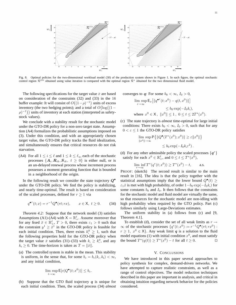
To illustrate how the regionR∗ must be modified to accountfor variability we consider the following two dimensionalMarkov Decision Process (MDP) workload model with stateprocessY , state spaceZ2, and one-step cost function equalto the effective cost onR2 illustrated at left in Figure 3. Thestate process is defined in discrete-time via,

Y (t + 1) = Y (t) + I(t) + N(t + 1), t ≥ 0, (30)

whereI is the two dimensional idleness process.The processN is i.i.d., and its marginal distribution is

supported on{(2, 0)T, (0, 2)T, (−5,−5)T}. Two cases wereconsidered. In Case I the marginal distribution is uniform(each possible value occurs with probability1/3.) This resultsin a mean drift given byE[N(t)] = −[1, 1]T. In Case 2 therespective probabilities are given by{43/240, 7/48, 31/120}.The mean drift is given byE[N(t)] = −[1, 1/10]T, which isconsistent with the drift vector shown in Figure 4. In eachcase, the second order statistics approximate the Central LimitTheorem variance obtained in a network with Poisson demand,and exponential servers.

The average-cost optimal policy is defined by a regionRSTO ⊂ Z

2 that determines the optimal idleness processI∗

as a function ofY . Shown in Figure 8 are the optimalregions obtained using value iteration in each of the two cases.Note that the boundaries ofRSTO are approximately affine, aspredicted by results in [6], [21].

Rather than compute the optimal policy for an MDP model,we propose here designs based on an affine enlargement ofthe coneRGTO used for the fluid model. All of the policiesconsidered in Sections 4.1-4.3 can be similarly modified.

We adopt the discrete-review structure described in [13] todefine the followingDiscrete-Review GTO policy. We supposethat a time horizonT > 0 is given, and the total allocation

z(T ) is obtained through a linear program. We then requirethat this total allocation is met by timeT , but the details ofthe allocation{z(t) : 0 ≤ t ≤ T } are not specified. With thisflexibility, it is possible to take into account the discretenatureof allocation decisions, and other issues such as set-up timesthat arise in manufacturing systems.

The affine enlargement ofRGTO is specified by a fixed targetvalue x ∈ R

`+. One goal in the GTO-DR policy introduced

next is to maintain the lower boundQ(t) ≥ x for all t. Forthis purpose a parameter0 < ε1 < 1 is fixed and, given aninitial conditionx0 ∈ X, a surrogate target value is defined by

x1 = x1(x0) := min(x, x0 + ε1x),

where the minimization is component-wise.

GTO-DR ALGORITHM Given the initial conditionx0; thetarget statex ∈ R

`+; planning horizonT > 0; and parameter

ε1 > 0, the GTO-DR control allocation is given byZ(T ) =ζ1∗T , where ζ1∗ is any optimizer to the following linearprogram:

min γ s. t. γ ≥ 〈ci, y1〉, i ∈ Ic(y1),

y1 = x0 + (Bζ1 + α)T1,y1 ≥ x1,x = y1 + (Bζ2 + α)T2,

ζ1, ζ2 ∈ U, y1 ∈ X, γ ∈ R,

whereT1 := min(T, T ∗(x0, x) ), andT2 := T ∗(x0, x) − T1.

The solutionζ1∗ of the linear program in GTO-DR coin-cides with the allocation rate obtained in the GTO policy (27)when the target statex is set to zero, and the planning horizonT is sufficiently small:

Proposition 4.1: Suppose thatx = θ in the GTO-DRpolicy. Then, for eachx0 ∈ X, there existsT > 0 sufficientlysmall such that the solutionζ1∗ ∈ U is a GTO allocation rateon [0, T ] with initial condition x0.

The GTO-DR policy is parameterized by the time horizonT , and the target-statex. For a given value ofT there aretwo major constraints to be taken into account on choosingthe target state:

(i) Starvation avoidance: For the fluid model, ifq(0) ≥ x,then each resource1 ≤ i ≤ `r◦ can work at capacityon the time-horizon[0, T ]. That is, there existsv ∈ V,satisfying

〈ξi, v〉 = −(1 − ρi), (31)

for 1 ≤ i ≤ `r◦, and x + Tv ∈ X. The following boundis suggested by results from [19], [2]: For some constantks > 0, and each1 ≤ i ≤ `m,

∑

j≥1

Ci,j xj ≥ ks log( 1

1 − ρ

), (32)

whereC is the constituency matrix.(ii) Appropriate hedging point: The resulting affine region

in workload space should be an appropriate enlargementof the fluid control regionRGTO: For a constantkh > 0,and each1 ≤ j ≤ `r◦,

wj := (Ξx)j ≤ −kh

( 1

1 − ρj

). (33)

11

w2

w1w1

w2

−(1 − ρ) −(1 − ρ)

R∗

R∗

20 10 0 10 20 30 40 50

20

10

0

10

20

30

40

50

20 10 0 10 20 30 40 50

20

10

0

10

20

30

40

50

R

RSTO

RSTO

Fig. 8. Optimal policies for the two-dimensional workload model (30) of the production system shown in Figure 1. In each figure, the optimal stochasticcontrol regionRSTO obtained using value iteration is compared with the optimalregionR∗ obtained for the two dimensional fluid model.

The following specifications for the target valuex are basedon consideration of the constraints (32) and (33) in the16buffer example: It will consist ofO

((1−ρ)−1

)units of excess

inventory (the two hedging points); and a total ofO(log

((1−

ρ)−1))

units of inventory at each station (interpreted as safety-stock values).

We conclude with a stability result for the stochastic modelunder the GTO-DR policy for a non-zero target state. Assump-tion (A4) formalizes the probabilistic assumptions imposed on(3). Under this condition, and with an appropriately chosentarget value, the GTO-DR policy tracks the fluid idealization,and simultaneously ensures that critical resources do not riskstarvation.

(A4) For all 1 ≤ i ≤ ` and1 ≤ k ≤ `u, each of the stochasticprocesses{Ai, Rik, Sik, t ≥ 0} is either null, or isan un-delayed renewal process whose increment processpossesses a moment generating function that is boundedin a neighborhood of the origin.

In the following result we consider the state trajectoryQ•

under the GTO-DR policy. We find the policy is stabilizing,and nearly time-optimal. The result is based on considerationof the scaled processes, defined forr ≥ 1 via

q•r(t; x) = r−1Q•(rt; rx), x ∈ X, t ≥ 0. (34)

Theorem 4.2: Suppose that the network model (3) satisfiesAssumptions (A1)-(A4) withX = R

`+. Assume moreover that

for any fixed x ∈ R`+, T > 0, there existsε1 > 0 such that

the constrainty1 ≥ x1 in the GTO-DR policy is feasible foreach initial condition. Then, there existsk0

s ≥ 1, such thatthe following properties hold for the GTO-DR policy whenthe target valuex satisfies (31)–(33) withks ≥ k0

s , and anykh ≥ 0. The time-horizon is taken asT = ‖x‖.

(a) The controlled system is stable in the mean. This stabilityis uniform, in the sense that, for somebc = bc(ks, kh) < ∞,and any initial condition,

lim supt→∞

E[c(Q•(t; x0))] ≤ bc.

(b) Suppose that the GTO fluid trajectoryq is unique foreach initial condition. Then, the scaled process (34)almost

converges toq: For someb0 < ∞, I0 > 0,

lim supr→∞

Ex

[‖q•r(t; x0) − q(t, x0)‖

]

≤ b0 exp(−I0ks),

where x0 ∈ X , ‖x0‖ ≤ 1 , 0 ≤ t ≤ 2T ∗(x0).

(c) The state trajectory isalmost time-optimal for large initialconditions: There existsb0 < ∞, I0 > 0, such that for any0 < ε ≤ 1 the GTO-DR policy satisfies

lim sup‖x0‖→∞

P{‖Q•(T ∗(x0); x0)‖ ≥ ε‖x0‖

}

≤ b0 exp(−I0ksε2) .

(d) For any other admissible policy the scaled processes{qr}satisfy for eachx0 ∈ R

`+, and0 ≤ t ≤ T ∗(x0),

lim infr→∞

T ∗(qr(t; x0)) ≥ T ∗(x0) − t, a.s.

PROOF: (sketch) The second result is similar to the mainresult in [16]. The idea is that the policy together with thestatistical assumptions imply that the lower boundQ•(t) ≥ε1x is met with high probability, of order1−b0 exp(−I0ks) forsome constantsb0 andI0. It then follows that the constraintsfor the stochastic model and fluid model are virtually the same,so that resources for the stochastic model are non-idling withhigh probability when required by the GTO policy. Part (c)follows similarly using Large-Deviations estimates.

The uniform stability in (a) follows from (c) and [9,Theorem 4.1].

To establish (d), consider the set of all weak limits asr →∞ of the stochastic processes{qr(t; x0) := r−1Q•(rt; rx0) :r ≥ 1, x0 ∈ X}. Any weak limit q is a solution to the fluidmodel equations (1) with initial conditionx0, and must satisfythe boundT ∗(q(t)) ≥ T ∗(x0) − t for all t ≥ 0. ut

V. CONCLUSIONS

We have introduced in this paper several approaches topolicy synthesis for complex, demand-driven networks. Wehave attempted to capture realistic constraints, as well asarange of control objectives. The model reduction techniquesdescribed in this paper are important in analysis, and critical inobtaining intuition regarding network behavior for the policiesconsidered.

12

Of course, there is also much room for further research.In our consideration of resource maintenance we assumed

complete information regarding down-time. An obvious nextstep is to investigate the impact of uncertainty on performancefor the algorithms described here, and to see if these algo-rithms can be improved given further statistical information.

It is natural to consider how these methods extend to mod-els with competing players, and distributed information. Anapplication of current interest concerns pricing and resourceallocation in power distribution. Those who design deregulatedmarkets can greatly benefit from a better understanding of theincentives in the network, which will eventually lead to a moreefficient market design. Some preliminary results are containedin [7].

Finally, we look forward to testing these policies in a real-world setting. We believe that the approaches described herewill have significant impact in network management for semi-conductor and related manufacturing industries.

REFERENCES

[1] F. Avram, D. Bertsimas, and M. Ricard. Fluid models of sequencingproblems in open queueing networks; an optimal control approach. InStochastic networks, volume 71 ofIMA Vol. Math. Appl., pages 199–234. Springer, New York, 1995.

[2] S.L. Bell and R.J. Williams. Dynamic scheduling of a system with twoparallel servers: Asymptotic optimality of a continuous review thesholdpolicy in heavy traffic. InProceedings of the 39th Conference onDecision and Control, pages 1743–1748, Pheonix, Arizona, 1999.

[3] M. Bramson. State space collapse with application to heavy trafficlimits for multiclass queueing networks.Queueing Systems: Theoriesand Applications, 30(89-148), 1998.

[4] H. Chen and A. Mandelbaum. Discrete flow networks: bottleneckanalysis and fluid approximations.Math. Oper. Res., 16(2):408–446,1991.

[5] H. Chen and David D. Yao. Fundamentals of queueing networks:Performance, asymptotics, and optimization. Springer-Verlag, New York,2001. Stochastic Modelling and Applied Probability.

[6] M. Chen, C. Pandit, and S.P. Meyn. In search of sensitivity in networkoptimization. Queueing Systems, 44(4):313–363, 2003.

[7] I.-K. Cho and S. P. Meyn The dynamics of the ancillary service pricesin power distribution systems. In preparation. Preliminary version inthe Proceedings of the 42nd IEEE Conference on Decision and Control,December 9-12, 2003.

[8] A.J. Clark and H.E. Scarf. Optimal policies for a multi-echelon inventoryproblem. Management Science, Vol. 6, No. 4, 1960.

[9] J.G. Dai and S.P. Meyn. Stability and convergence of moments formulticlass queueing networks via fluid limit models.IEEE Transactionson Automatic Control, 40:1889–1904, 1995.

[10] J.G. Dai and G. Weiss. A fluid heuristic for minimizing makespan injob shops.Oper. Res., 50(4):692–707, 2002.

[11] R. Dubrawski. Myopic and far-sighted strategies for control of demand-driven networks. Masters thesis, Department of ElectricalEngineering,UIUC, 2000. Urbana, Illinois, USA.

[12] S.B. Gershwin. Manufacturing Systems Engineering. Prentice–Hall,Englewood Cliffs, NJ, 1993.

[13] J.M. Harrison. The BIGSTEP approach to flow management in stochas-tic processing networks. In F. P. Kelly, S. Zachary, and I. Ziedins,editors, Stochastic Networks: Theory and Applications, pages 57–90.Oxford Science Publications, Oxford U.K., 1996.

[14] J.M. Harrison and J.A. Van Mieghem. Dynamic control of Browniannetworks: state space collapse and equivalent workload formulations.Ann. Appl. Probab., 7(3):747–771, 1997.

[15] S.G. Henderson, S. P. Meyn, and V. Tadic. Performance evaluationand policy selection in multiclass networks.Discrete Event DynamicSystems: Theory and Applications, 13:149–189, 2003. Special issue onlearning and optimization methods (invited).

[16] C. Maglaras. Dynamic scheduling in multiclass queueing networks:Stability under discrete-review policies.Queueing Systems, 31:171–206,1999.

[17] S.P. Meyn. Stability and optimization of queueing networks and theirfluid models. In Mathematics of stochastic manufacturing systems(Williamsburg, VA, 1996), pages 175–199. Amer. Math. Soc., Provi-dence, RI, 1997.

[18] S.P. Meyn. Sequencing and routing in multiclass queueing networks.Part I: Feedback regulation.SIAM J. Control Optim., 40(3):741–776,2001.

[19] S. P. Meyn. Sequencing and routing in multiclass queueing networks.Part II: Workload relaxations.SIAM J. Control Optim., 42(1):178–217,2003.

[20] S. P. Meyn. Dynamic safety-stocks for asymptotic optimality instochastic networks. (submitted for publication), 2003.

[21] S.P. Meyn. Value functions, optimization, and performance evaluationin stochastic network models. (submitted for publication), 2003.

[22] J.K. Robinson, J.W. Fowler, and E. Neacy. Capacity lossfactorsin semiconductor manufacturing. Working paper, availablefromwww.FabTime.com.

[23] A. Sharifnia. Production control of a manufacturing system with multiplemachine states.IEEE Transactions on Automatic Control, 33:600–626,July 1988.

[24] G. Weiss. Optimal draining of a fluid re-entrant line. InFrank Kellyand Ruth Williams, editors,Volume 71 of IMA volumes in Mathematicsand its Applications, pages 91–103, New York, 1995. Springer-Verlag.

PLACEPHOTOHERE

Richard Dubrawski was born in Pittsburgh, PA in1967. He obtained a BSEE from The PennsylvaniaState University in 1998 and an MSEE from UIUCin 2000. He is currently working at Viasat in SanDiego as a senior Software Engineer.

PLACEPHOTOHERE

Mike Chen was born in Kaohsiung City, Taiwan in1976. He obtained a BEng from McGill Universityin 1999 and an MS from UIUC in 2002, both inElectrical and Computer Engineering. He plans tocomplete a PhD in Electrical and Computer Engi-neering and an MS in Mathematics at UIUC in April,2005.

PLACEPHOTOHERE

Sean P. Meyn received the B.A. degree in Math-ematics Summa Cum Laude from UCLA in 1982,and the PhD degree in Electrical Engineering fromMcGill University in 1987. After a two year postdoc-toral fellowship at the Australian National Universityin Canberra, Dr. Meyn and his family moved tothe Midwest. He is now a Professor at the Depart-ment of Electrical and Computer Engineering, anda Research Professor at the Coordinated ScienceLaboratory at the University of Illinois.

Dr. Meyn has served on the editorial boards ofseveral journals in the systems and control, and applied probability areas. Heis coauthor with Richard L. Tweedie of the monographMarkov Chains andStochastic Stability, Springer-Verlag, London, 1993; and received jointly withTweedie the1994 ORSA/TIMS Best Publication In Applied Probability Award.