Embed Size (px)
Citation preview
3 Magnetism in Correlated Matter
Eva PavariniInstitute for Advanced SimulationForschungszentrum Julich
Contents1 Overview 2
2 The Hubbard model 82.1 Weak-correlation limit . . . . . . . . . . . . . . . . . . . . . . . . . . . . . . 122.2 Atomic limit . . . . . . . . . . . . . . . . . . . . . . . . . . . . . . . . . . . . 202.3 Strong-correlation limit . . . . . . . . . . . . . . . . . . . . . . . . . . . . . . 24
3 The Anderson model 363.1 The Kondo limit . . . . . . . . . . . . . . . . . . . . . . . . . . . . . . . . . . 363.2 The RKKY interaction . . . . . . . . . . . . . . . . . . . . . . . . . . . . . . 41
4 Conclusion 42
A Formalism 44A.1 Matsubara Green functions . . . . . . . . . . . . . . . . . . . . . . . . . . . . 44A.2 Linear-response theory . . . . . . . . . . . . . . . . . . . . . . . . . . . . . . 47A.3 Magnetic susceptibility . . . . . . . . . . . . . . . . . . . . . . . . . . . . . . 49
E. Pavarini, E. Koch, and P. Coleman (eds.)Many-Body Physics: From Kondo to HubbardModeling and Simulation Vol. 5Forschungszentrum Julich, 2015, ISBN 978-3-95806-074-6http://www.cond-mat.de/events/correl15
3.2 Eva Pavarini
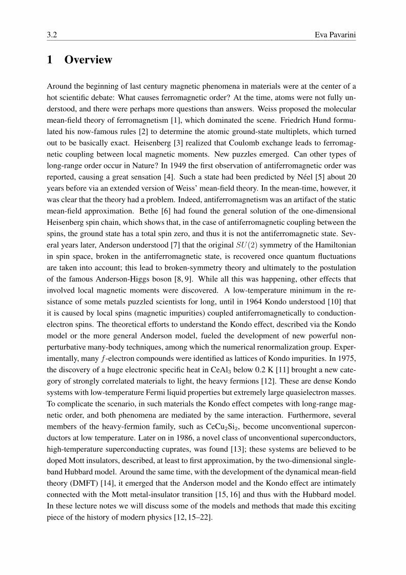
1 Overview
Around the beginning of last century magnetic phenomena in materials were at the center of ahot scientific debate: What causes ferromagnetic order? At the time, atoms were not fully un-derstood, and there were perhaps more questions than answers. Weiss proposed the molecularmean-field theory of ferromagnetism [1], which dominated the scene. Friedrich Hund formu-lated his now-famous rules [2] to determine the atomic ground-state multiplets, which turnedout to be basically exact. Heisenberg [3] realized that Coulomb exchange leads to ferromag-netic coupling between local magnetic moments. New puzzles emerged. Can other types oflong-range order occur in Nature? In 1949 the first observation of antiferromagnetic order wasreported, causing a great sensation [4]. Such a state had been predicted by Neel [5] about 20years before via an extended version of Weiss’ mean-field theory. In the mean-time, however, itwas clear that the theory had a problem. Indeed, antiferromagnetism was an artifact of the staticmean-field approximation. Bethe [6] had found the general solution of the one-dimensionalHeisenberg spin chain, which shows that, in the case of antiferromagnetic coupling between thespins, the ground state has a total spin zero, and thus it is not the antiferromagnetic state. Sev-eral years later, Anderson understood [7] that the original SU(2) symmetry of the Hamiltonianin spin space, broken in the antiferromagnetic state, is recovered once quantum fluctuationsare taken into account; this lead to broken-symmetry theory and ultimately to the postulationof the famous Anderson-Higgs boson [8, 9]. While all this was happening, other effects thatinvolved local magnetic moments were discovered. A low-temperature minimum in the re-sistance of some metals puzzled scientists for long, until in 1964 Kondo understood [10] thatit is caused by local spins (magnetic impurities) coupled antiferromagnetically to conduction-electron spins. The theoretical efforts to understand the Kondo effect, described via the Kondomodel or the more general Anderson model, fueled the development of new powerful non-perturbative many-body techniques, among which the numerical renormalization group. Exper-imentally, many f -electron compounds were identified as lattices of Kondo impurities. In 1975,the discovery of a huge electronic specific heat in CeAl3 below 0.2 K [11] brought a new cate-gory of strongly correlated materials to light, the heavy fermions [12]. These are dense Kondosystems with low-temperature Fermi liquid properties but extremely large quasielectron masses.To complicate the scenario, in such materials the Kondo effect competes with long-range mag-netic order, and both phenomena are mediated by the same interaction. Furthermore, severalmembers of the heavy-fermion family, such as CeCu2Si2, become unconventional supercon-ductors at low temperature. Later on in 1986, a novel class of unconventional superconductors,high-temperature superconducting cuprates, was found [13]; these systems are believed to bedoped Mott insulators, described, at least to first approximation, by the two-dimensional single-band Hubbard model. Around the same time, with the development of the dynamical mean-fieldtheory (DMFT) [14], it emerged that the Anderson model and the Kondo effect are intimatelyconnected with the Mott metal-insulator transition [15, 16] and thus with the Hubbard model.In these lecture notes we will discuss some of the models and methods that made this excitingpiece of the history of modern physics [12, 15–22].
Magnetism in Correlated Matter 3.3
Magnetism ultimately arises from the intrinsic magnetic moment of electrons, µ = −gµBs,where µB is the Bohr magneton and g ' 2.0023 is the electronic g-factor. It is, however,an inherently quantum mechanical effect, the consequence of the interplay between the Pauliexclusion principle, the Coulomb electron-electron interaction, and the hopping of electrons.To understand this let us consider the simplest possible system, an isolated atom or ion. In thenon-relativistic limit electrons in a single ion are typically described by the Hamiltonian
HNRe = −1
2
∑i
∇2i −
∑i
Z
ri+∑i>j
1
|ri − rj|,
where Z is the atomic number and {ri} are the coordinates of the electrons with respect to theionic nucleus. Here, as in the rest of this lecture, we use atomic units. If we consider only theexternal atomic shell with quantum numbers nl, for example the 3d shell of transition-metalions, we can rewrite this Hamiltonian as follows
HNRe = εnl
∑mσ
c†mσcmσ +1
2
∑σσ′
∑mmm′m′
U lmm′mm′c
†mσc
†m′σ′cm′σ′cmσ. (1)
The parameter εnl is the energy of the electrons in the nl atomic shell and m the degenerateone-electron states in that shell. For a hydrogen-like atom
εnl = −1
2
Z2
n2.
The couplings U lmm′mm′ are the four-index Coulomb integrals. In a basis of atomic functions
the bare Coulomb integrals are
U iji′j′
mm′mm′ =
∫dr1
∫dr2
ψimσ(r1)ψjm′σ′(r2)ψj′m′σ′(r2)ψi′mσ(r1)
|r1 − r2|,
and U lmm′mm′ = U iiii
mm′mm′ , where m,m′, m, m′ ∈ nl shell. The eigenstates of Hamiltonian (1)for fixed number of electronsN are the multiplets [23,24]. Since inHNR
e the Coulomb repulsionand the central potential are the only interactions, the multiplets can be labeled with S and L,the quantum numbers of the electronic total spin and total orbital angular momentum operators,S =
∑i si, and L =
∑i li. Closed-shell ions have S = L = 0 in their ground state. Ions
with a partially-filled shell are called magnetic ions; the value of S and L for their ground statecan be obtained via Hund’s rules. The first and second Hund’s rules say that the lowest-energymultiplet is the one with
1. the largest value of S
2. the largest value of L compatible with the previous rule
The main relativistic effect is the spin-orbit interaction, which has the form HSOe =
∑i λi li·si.
For not-too-heavy atoms it is a weak perturbation. For electrons in a given shell, we can rewriteHSOe in a simpler manner using the first and second Hund’s rule. If the shell filling is n < 1/2,
3.4 Eva Pavarini
the ground-state multiplet has spin S = (2l + 1)n = N/2; thus si = S/N = S/2S. If,instead, n > 1/2, since the sum of li vanishes for the electrons with spin parallel to S, onlythe electrons with spin antiparallel to S contribute. Their spin is si = −S/Nu = −S/2Swhere Nu = 2(2l + 1)(1− n) is the number of unpaired electrons. We therefore obtain the LSHamiltonian
HSOe ∼
[2Θ(1− 2n)− 1
]gµ2
B
2S
⟨1
r
d
drvR(r)
⟩︸ ︷︷ ︸
λ
L · S = λ L · S, (2)
where Θ is the Heaviside step function and vR(r) is the effective potential, which includes, e.g.,the Hartree electron-electron term [25]. For a hydrogen-like atom, vR(r) = −Z/r. Because ofthe LS coupling (2) the eigenstates have quantum numbers L, S and J , where J = S+L is thetotal angular momentum. Since L · S = [J2 −L2 − S2] /2, the value of J in the ground-statemultiplet is thus (third Hund’s rule)
• total angular momentum J =
|L− S| for filling n < 1/2
S for filling n = 1/2
L+ S for filling n > 1/2
In the presence of spin-orbit interaction a given multiplet is then labeled by 2S+1LJ , and itsstates can be indicated as |JJzLS〉. If we consider, e.g., the case of the Cu2+ ion, characterizedby the [Ar] 3d9 electronic configuration, Hund’s rules tell us that the 3d ground-state multiplethas quantum numbers S = 1/2, L = 2 and J = 5/2. A Mn3+ ion, which is in the [Ar] 3d4
electronic configuration, has instead a ground-state multiplet with quantum numbers S = 2,L = 2 and J = 0. The order of the Hund’s rules reflects the hierarchy of the interactions. Thestrongest interactions are the potential vR(r), which determines εnl, and the average Coulombinteraction, the strength of which is measured by the average direct Coulomb integral,
Uavg =1
(2l + 1)2
∑mm′
U lmm′mm′ .
For an N -electron state the energy associated with these two interactions is E(N) = εnlN +
UavgN(N − 1)/2, the same for all multiplets of a given shell. The first Hund’s rule is insteaddue to the average exchange Coulomb integral, Javg, defined as
Uavg − Javg =1
2l(2l + 1)
∑mm′
(U lmm′mm′ − U l
mm′m′m
),
which is the second-largest Coulomb term; for transition-metal ions Javg ∼ 1 eV. SmallerCoulomb integrals determine the orbital anisotropy of the Coulomb matrix and the secondHund’s rule.1 The third Hund’s rule comes, as we have seen, from the spin-orbit interactionwhich, for not-too-heavy atoms, is significantly weaker than all the rest.
1For more details on Coulomb integrals and their averages see Ref. [25].
Magnetism in Correlated Matter 3.5
The role of Coulomb electron-electron interaction in determining S and L can be understoodthrough the simple example of a C atom, electronic configuration [He] 2s2 2p2. We consideronly the p shell, filled by two electrons. The Coulomb exchange integrals have the form
Jpm,m′ = Upmm′m′m =
∫dr1
∫dr2
ψimσ(r1)ψim′σ(r2)ψimσ(r2)ψim′σ(r1)
|r1 − r2|
=
∫dr1
∫dr2
φimm′σ(r1)φimm′σ(r2)
|r1 − r2|. (3)
If we express the Coulomb potential as
1
|r1 − r2|=
1
V
∑k
4π
k2eik·(r1−r2),
we can rewrite the Coulomb exchange integrals in a form that shows immediately that they arealways positive
Jpm,m′ =1
V
∑k
4π
k2|φimm′σ(k)|2 > 0.
They generate the Coulomb-interaction term
−1
2
∑σ
∑m6=m′
Jpm,m′c†mσcmσc
†m′σcm′σ = −1
2
∑m6=m′
2Jpm,m′
[Smz S
m′
z +1
4nmnm′
].
This exchange interaction yields an energy gain if the two electrons occupy two different porbitals with parallel spins, hence it favors the state with the largest spin (first Hund’s rule). Itturns out that for the p2 configuration there is only one possible multiplet with S = 1, and sucha state has L = 1. There are instead two excited S = 0 multiplets, one with L = 0 and the otherwith L = 2; the latter is the one with lower energy (second Hund’s rule).To understand the magnetic properties of an isolated ion we have to analyze how its levels aremodified by an external magnetic field h. The effect of a magnetic field is described by
HHe = µB (gS +L) · h+
h2
8
∑i
(x2i + y2
i
)= HZ
e +HLe . (4)
The linear term is the Zeeman Hamiltonian. If the ground-state multiplet is characterized byJ 6= 0 the Zeeman interaction splits its 2J + 1 degenerate levels. The second-order term yieldsLarmor diamagnetism, which is usually only important if the ground-state multiplet has J = 0,as happens for ions with closed external shells. The energy µBh is typically very small (for afield as large as 100 T it is as small as 6 meV); it can however be comparable with or largerthan the spin-orbit interaction if the latter is tiny (very light atoms). Taking all interactions intoaccount, the total Hamiltonian is
He ∼ HNRe +HSO
e +HHe .
3.6 Eva Pavarini
In a crystal the electronic Hamiltonian is complicated by the interaction with other nuclei andtheir electrons. The non-relativistic part of the Hamiltonian then takes the form
HNRe = −1
2
∑i
∇2i +
1
2
∑i6=i′
1
|ri − ri′ |−∑iα
Zα|ri −Rα|
+1
2
∑α6=α′
ZαZα′
|Rα −Rα′ |,
where Zα is the atomic number of the nucleus located at position Rα. In a basis of localizedWannier functions [25] this Hamiltonian can be written as
HNRe = −
∑ii′σ
∑mm′
ti,i′
m,m′c†imσci′m′σ +
1
2
∑ii′jj′
∑σσ′
∑mm′
∑mm′
U iji′j′
mm′mm′c†imσc
†jm′σ′cj′m′σ′ci′mσ, (5)
where
ti,i′
m,m′ = −∫dr ψimσ(r)
[−1
2∇2 + vR(r)
]ψi′m′σ(r).
The terms εm,m′ = −ti,im,m′ yield the crystal-field matrix and ti,i′
m,m′ with i 6= i′ the hoppingintegrals. The label m indicates here the orbital quantum number of the Wannier function. Ingeneral, the Hamiltonian (5) will include states stemming from more than a single atomic shell.For example, in the case of strongly correlated transition-metal oxides, the set {im} includestransition-metal 3d and oxygen 2p states. The exact solution of the many-body problem de-scribed by (5) is an impossible challenge. The reason is that the properties of a many-bodysystem are inherently emergent and hence hard to predict ab-initio in the absence of any un-derstanding of the mechanism behind them. In this lecture, however, we want to focus onmagnetism. Since the nature of cooperative magnetic phenomena in crystals is currently to alarge extent understood, we can find realistic approximations to (5) and even map it onto simplermodels that still retain the essential ingredients to explain long-range magnetic order.Let us identify the parameters of the electronic Hamiltonian important for magnetism. The firstis the crystal-field matrix εm,m′ . The crystal field at a given site i is a non-spherical potentialdue to the joint effect of the electric field generated by the surrounding ions and of covalent-bond formation [24]. The crystal field can split the levels within a given shell and thereforehas a strong impact on magnetic properties. We can identify three ideal regimes. In the strong-crystal-field limit the crystal-field splitting is so large that it is comparable with the averageCoulomb exchange responsible for the first Hund’s rule. This can happen in 4d or 5d transition-metal oxides. A consequence of an intermediate crystal field (weaker than the average Coulombexchange but larger than Coulomb anisotropy and spin-orbit interaction) is the quenching of theangular momentum, 〈L〉 = 0. In this limit the second and third Hund’s rule are not respected.This typically happens in 3d transition-metal oxides. In 4f systems the crystal-field splittingis usually much weaker than the spin-orbit coupling (weak-crystal-field limit) and mainly splitsstates within a given multiplet, leaving a reduced magnetic moment. In all three cases, becauseof the crystal field, a magnetic ion in a crystal might lose – totally or partially – its spin, itsangular momentum, or its total momentum. Or, sometimes, it is the other way around. Thishappens for Mn3+ ions, which should have a J = 0 ground state according to the third Hund’srule. In the perovskite LaMnO3, however, they behave as S = 2 ions because of the quenchingof the angular momentum.
Magnetism in Correlated Matter 3.7
Even if the crystal field does not suppress the magnetic moment of the ion, the electrons mightdelocalize to form broad bands, completely losing their original atomic character. This happens,e.g., if the hopping integrals ti,i
′
m,m′ are much larger than the average on-site Coulomb interactionUavg. Surprisingly, magnetic instabilities arise even in the absence of localized moments. Thisitinerant magnetism is mostly due to band effects, i.e., it is associated with a large one-electronlinear static response-function χ0(q; 0). In this limit correlation effects are typically weak. Tostudy them we can exploit the power of the standard model of solid-state physics, the density-functional theory (DFT), taking into account Coulomb interaction effects beyond the local-density approximation (LDA) at the perturbative level, e.g., in the random-phase approximation(RPA). With this approach we can understand and describe Stoner instabilities.In the opposite limit, the local-moments regime, the hopping integrals are small with respectto Uavg. This is the regime of strong electron-electron correlations, where complex many-bodyeffects, e.g., those leading to the Mott metal-insulator transition, play an important role. At lowenough energy, however, only spins and spin-spin interactions matter. Ultimately, at integerfilling we can integrate out (downfold) charge fluctuations and describe the system via effectivespin Hamiltonians. The latter typically take the form
HS =1
2
∑ii′
Γ i,i′ Si · Si′ + · · · = HHS + . . . . (6)
The term HHS given explicitly in (6) is the Heisenberg Hamiltonian, and Γ i,i′ is the Heisenberg
exchange coupling, which can be antiferromagnetic (Γ i,i′ > 0) or ferromagnetic (Γ i,i′ < 0).The Hamiltonian (6) can, for a specific system, be quite complicated, and might include long-range exchange interactions or anisotropic terms. Nevertheless, it represents a huge simplifica-tion compared to the unsolvable many-body problem described by (5), since, at least within verygood approximation schemes, it can be solved. Spin Hamiltonians of type (6) are the minimalmodels that still provide a realistic picture of long-range magnetic order in strongly correlatedinsulators. There are various sources of exchange couplings. Electron-electron repulsion itselfyields, via Coulomb exchange, a ferromagnetic Heisenberg interaction, the Coulomb exchangeinteraction. The origin of such interaction can be understood via a simple model with a singleorbital, m. The inter-site Coulomb exchange coupling has then the form
J i,i′= U ii′i′i
mmmm =
∫dr1
∫dr2
ψimσ(r1)ψi′mσ(r2)ψimσ(r2)ψi′mσ(r1)
|r1 − r2|,
and it is therefore positive, as one can show by following the same steps that we used in Eq. (3)for Jpm,m′ . Hence, the corresponding Coulomb interaction yields a ferromagnetic Heisenberg-like Hamiltonian with
Γ i,i′ = −2J i,i′ < 0.
A different source of magnetic interactions are the kinetic exchange mechanisms (direct ex-change, super-exchange, double exchange, Ruderman-Kittel-Kasuya-Yosida interaction . . . ),which are mediated by the hopping integrals. Kinetic exchange couplings are typically (with
3.8 Eva Pavarini
a few well understood exceptions) antiferromagnetic [26]. A representative example of kineticexchange will be discussed in the next section.While the itinerant and local-moment regime are very interesting ideal limiting cases, correlatedmaterials elude rigid classifications. The same system can present features associated withboth regimes, although at different temperatures and/or energy scales. This happens in Kondosystems, heavy fermions, metallic strongly correlated materials, and doped Mott insulators.In this lecture we will discuss in representative cases the itinerant and localized-moment regimeand their crossover, as well as the most common mechanisms leading to magnetic cooperativephenomena. Since our target is to understand strongly correlated materials, we adopt the for-malism typically used for these systems. A concise introduction to Matsubara Green functions,correlation functions, susceptibilities, and linear-response theory can be found in the Appendix.
2 The Hubbard model
The simplest model that we can consider is the one-band Hubbard model
H = εd∑i
∑σ
c†iσciσ︸ ︷︷ ︸Hd
−t∑〈ii′〉
∑σ
c†iσci′σ︸ ︷︷ ︸HT
+U∑i
ni↑ni↓︸ ︷︷ ︸HU
= Hd +HT +HU , (7)
where εd is the on-site energy, t is the hopping integral between first-nearest neighbors 〈ii′〉, andU the on-site Coulomb repulsion; c†iσ creates an electron in a Wannier state with spin σ centeredat site i, and niσ = c†iσciσ. The Hubbard model is a simplified version of Hamiltonian (5) withm = m′ = m = m′ = 1 and
εd = −ti,i1,1
t = t〈i,i′〉1,1
U = U iiii1111
.
In the U = 0 limit the Hubbard model describes a system of independent electrons. TheHamiltonian is then diagonal in the Bloch basis
Hd +HT =∑kσ
[εd + εk
]c†kσckσ. (8)
The energy dispersion εk depends on the geometry and dimensionality d of the lattice. For ahypercubic lattice of dimension d
εk = −2td∑
ν=1
cos(krνa),
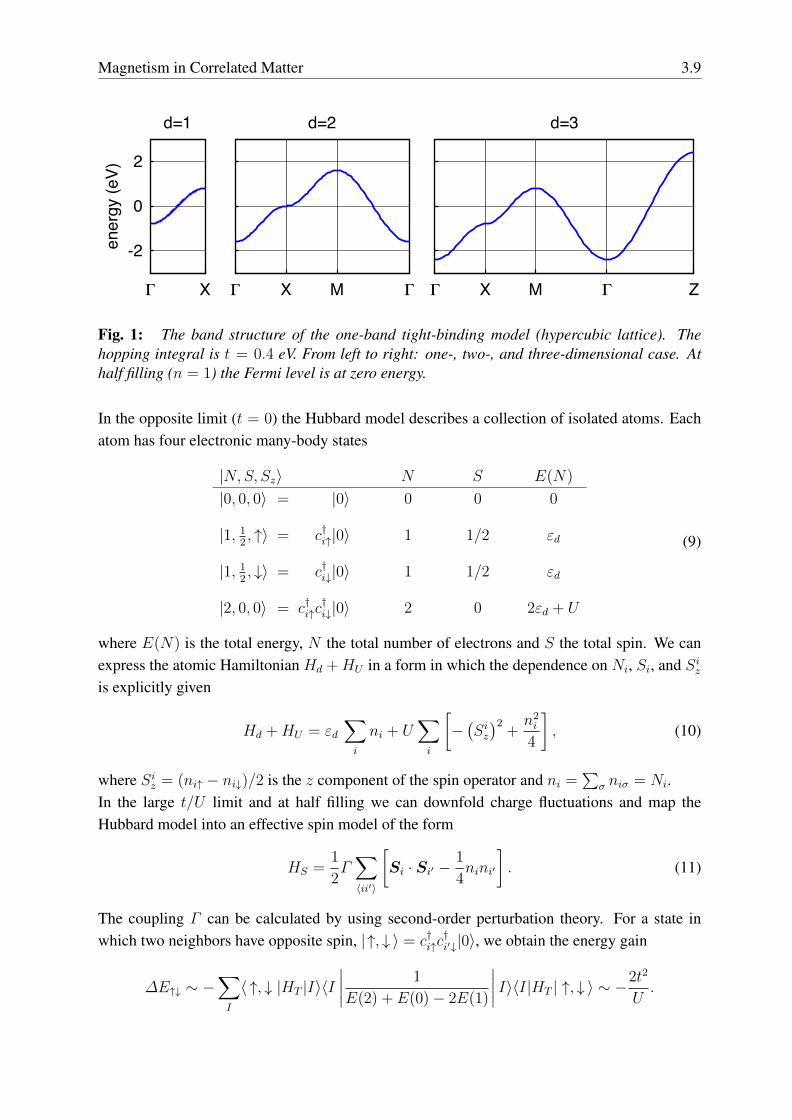
where a is the lattice constant, and r1 = x, r2 = y, r3 = z. The energy εk does not depend onthe spin. In Fig. 1 we show εk in the one-, two- and three-dimensional cases.
Magnetism in Correlated Matter 3.9
-2
0
2
Γ X
ener
gy (e
V)d=1
Γ X M Γ
d=2
Γ X M Γ Z
d=3
Fig. 1: The band structure of the one-band tight-binding model (hypercubic lattice). Thehopping integral is t = 0.4 eV. From left to right: one-, two-, and three-dimensional case. Athalf filling (n = 1) the Fermi level is at zero energy.
In the opposite limit (t = 0) the Hubbard model describes a collection of isolated atoms. Eachatom has four electronic many-body states
|N,S, Sz〉 N S E(N)
|0, 0, 0〉 = |0〉 0 0 0
|1, 12, ↑〉 = c†i↑|0〉 1 1/2 εd
|1, 12, ↓〉 = c†i↓|0〉 1 1/2 εd
|2, 0, 0〉 = c†i↑c†i↓|0〉 2 0 2εd + U
(9)
where E(N) is the total energy, N the total number of electrons and S the total spin. We canexpress the atomic Hamiltonian Hd +HU in a form in which the dependence on Ni, Si, and Sizis explicitly given
Hd +HU = εd∑i
ni + U∑i
[−(Siz)2
+n2i
4
], (10)
where Siz = (ni↑ − ni↓)/2 is the z component of the spin operator and ni =∑
σ niσ = Ni.In the large t/U limit and at half filling we can downfold charge fluctuations and map theHubbard model into an effective spin model of the form
HS =1
2Γ∑〈ii′〉
[Si · Si′ −
1
4nini′
]. (11)
The coupling Γ can be calculated by using second-order perturbation theory. For a state inwhich two neighbors have opposite spin, |↑, ↓ 〉 = c†i↑c
†i′↓|0〉, we obtain the energy gain
∆E↑↓ ∼ −∑I
〈 ↑, ↓ |HT |I〉〈I∣∣∣∣ 1
E(2) + E(0)− 2E(1)
∣∣∣∣ I〉〈I|HT | ↑, ↓ 〉 ∼ −2t2
U.
3.10 Eva Pavarini
Here |I〉 ranges over the excited states with one of the two neighboring sites doubly occupiedand the other empty, | ↑↓, 0〉 = c†i↑c
†i↓|0〉, or |0, ↑↓ 〉 = c†i′↑c
†i′↓|0〉; these states can be occupied
via virtual hopping processes. For a state in which two neighbors have parallel spins, | ↑, ↑ 〉 =c†i↑c
†i′↑|0〉, no virtual hopping is possible because of the Pauli principle, and ∆E↑↑ = 0. Thus
1
2Γ ∼ (∆E↑↑ −∆E↑↓) =
1
2
4t2
U. (12)
The exchange coupling Γ = 4t2/U is positive, i.e., antiferromagnetic.Canonical transformations [28] provide a scheme for deriving the effective spin model system-atically at any perturbation order. Let us consider a unitary transformation of the Hamiltonian
HS = eiSHe−iS = H + [iS,H] +1
2
[iS, [iS,H]
]+ . . . .
We search for a transformation operator that eliminates, at a given order, hopping integralsbetween states with a different number of doubly occupied states. To do this, first we split thekinetic term HT into a component H0
T that does not change the number of doubly occupiedstates and two terms that either increase it (H+
T ) or decrease it (H−T ) by one
HT = −t∑〈ii′〉
∑σ
c†iσci′σ = H0T +H+
T +H−T ,
where
H0T = −t
∑〈ii′〉
∑σ
ni−σ c†iσci′σ ni′−σ − t
∑〈ii′〉
∑σ
[1− ni−σ
]c†iσci′σ
[1− ni′−σ
],
H+T = −t
∑〈ii′〉
∑σ
ni−σ c†iσci′σ
[1− ni′−σ
],
H−T =(H+T
)†.
The term H0T commutes with HU . The remaining two terms fulfill the commutation rules
[H±T , HU ] = ∓UH±T .
The operator S can be expressed as a linear combination of powers of the three operatorsH0T , H
+T , and H−T . The actual combination, which gives the effective spin model at a given
order, can be found via a recursive procedure [28]. At half filling and second order, however,we can simply guess the form of S that leads to the Hamiltonian (11). By defining
S = − i
U
(H+T −H−T
)we obtain
HS = HU +H0T +
1
U
( [H+T , H
−T
]+[H0T , H
−T
]+[H+T , H
0T
] )+O(U−2).
Magnetism in Correlated Matter 3.11
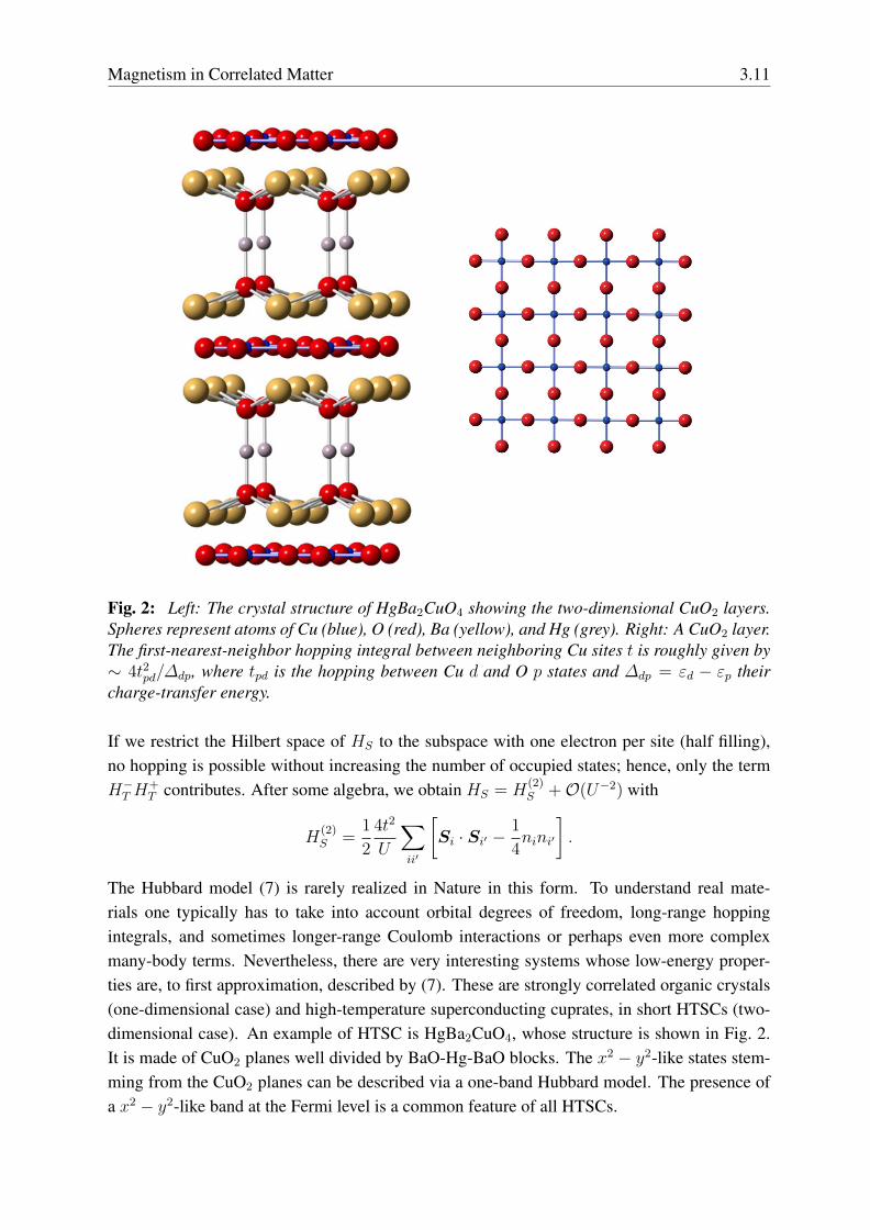
Fig. 2: Left: The crystal structure of HgBa2CuO4 showing the two-dimensional CuO2 layers.Spheres represent atoms of Cu (blue), O (red), Ba (yellow), and Hg (grey). Right: A CuO2 layer.The first-nearest-neighbor hopping integral between neighboring Cu sites t is roughly given by∼ 4t2pd/∆dp, where tpd is the hopping between Cu d and O p states and ∆dp = εd − εp theircharge-transfer energy.
If we restrict the Hilbert space of HS to the subspace with one electron per site (half filling),no hopping is possible without increasing the number of occupied states; hence, only the termH−T H
+T contributes. After some algebra, we obtain HS = H
(2)S +O(U−2) with
H(2)S =
1
2
4t2
U
∑ii′
[Si · Si′ −
1
4nini′
].
The Hubbard model (7) is rarely realized in Nature in this form. To understand real mate-rials one typically has to take into account orbital degrees of freedom, long-range hoppingintegrals, and sometimes longer-range Coulomb interactions or perhaps even more complexmany-body terms. Nevertheless, there are very interesting systems whose low-energy proper-ties are, to first approximation, described by (7). These are strongly correlated organic crystals(one-dimensional case) and high-temperature superconducting cuprates, in short HTSCs (two-dimensional case). An example of HTSC is HgBa2CuO4, whose structure is shown in Fig. 2.It is made of CuO2 planes well divided by BaO-Hg-BaO blocks. The x2 − y2-like states stem-ming from the CuO2 planes can be described via a one-band Hubbard model. The presence ofa x2 − y2-like band at the Fermi level is a common feature of all HTSCs.
3.12 Eva Pavarini
0
1
-2 0 2
DO
S
d=1
-2 0 2
energy (eV)
d=2
-2 0 2
d=3
0
1
2000 4000
χ R
d=1
2000 4000
T (K)
d=2
2000 4000
d=3
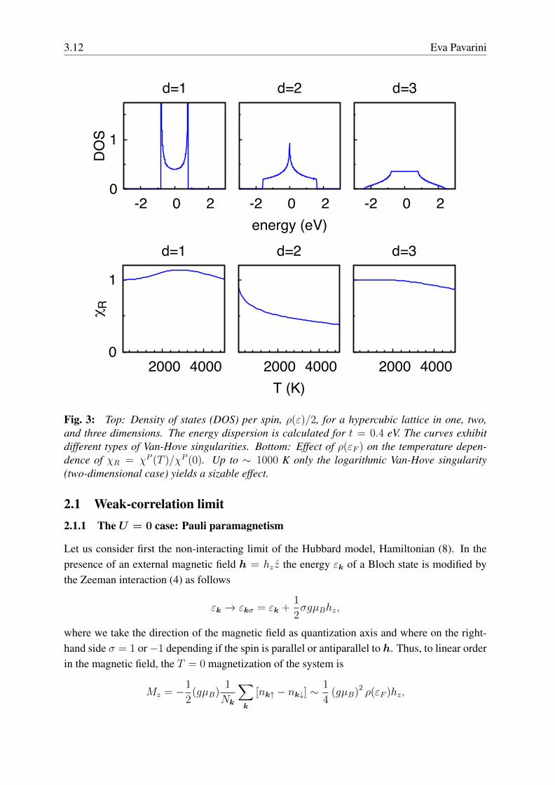
Fig. 3: Top: Density of states (DOS) per spin, ρ(ε)/2, for a hypercubic lattice in one, two,and three dimensions. The energy dispersion is calculated for t = 0.4 eV. The curves exhibitdifferent types of Van-Hove singularities. Bottom: Effect of ρ(εF ) on the temperature depen-dence of χR = χP (T )/χP (0). Up to ∼ 1000 K only the logarithmic Van-Hove singularity(two-dimensional case) yields a sizable effect.
2.1 Weak-correlation limit2.1.1 The U = 0 case: Pauli paramagnetism
Let us consider first the non-interacting limit of the Hubbard model, Hamiltonian (8). In thepresence of an external magnetic field h = hz z the energy εk of a Bloch state is modified bythe Zeeman interaction (4) as follows
εk → εkσ = εk +1
2σgµBhz,
where we take the direction of the magnetic field as quantization axis and where on the right-hand side σ = 1 or−1 depending if the spin is parallel or antiparallel to h. Thus, to linear orderin the magnetic field, the T = 0 magnetization of the system is
Mz = −1
2(gµB)
1
Nk
∑k
[nk↑ − nk↓] ∼1
4(gµB)
2 ρ(εF )hz,
Magnetism in Correlated Matter 3.13
l
m
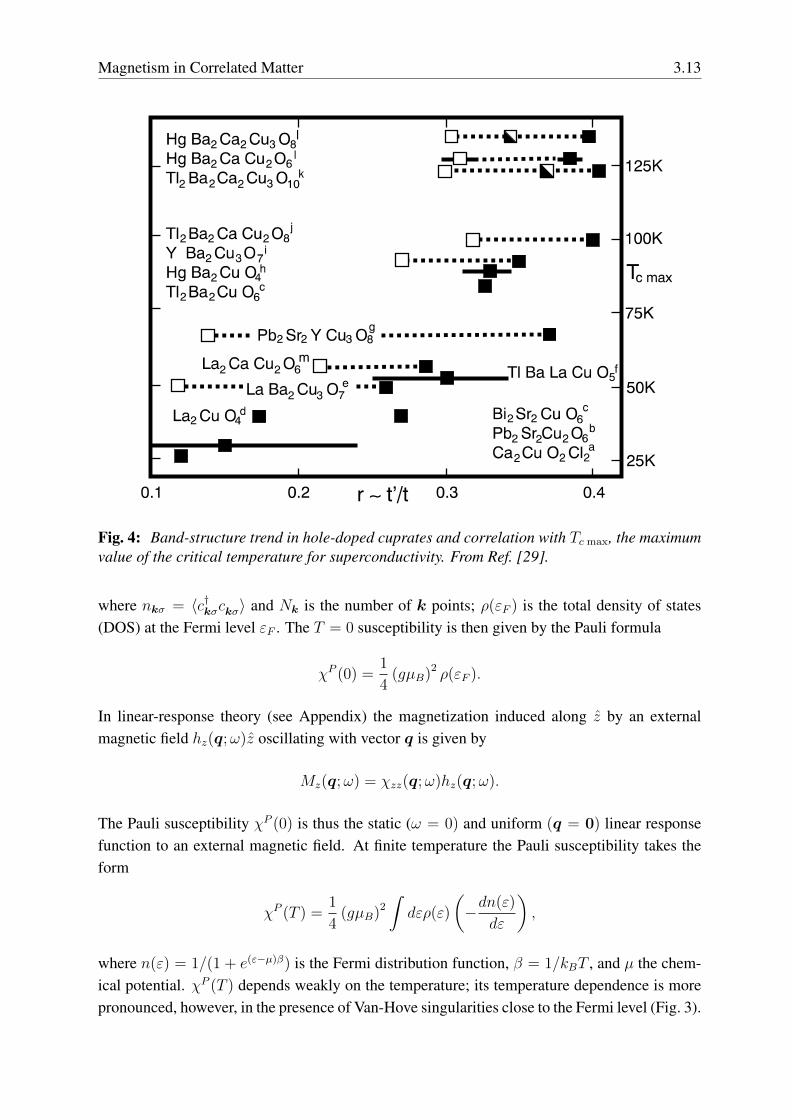
Fig. 4: Band-structure trend in hole-doped cuprates and correlation with Tc max, the maximumvalue of the critical temperature for superconductivity. From Ref. [29].
where nkσ = 〈c†kσckσ〉 and Nk is the number of k points; ρ(εF ) is the total density of states(DOS) at the Fermi level εF . The T = 0 susceptibility is then given by the Pauli formula
χP (0) =1
4(gµB)
2 ρ(εF ).
In linear-response theory (see Appendix) the magnetization induced along z by an externalmagnetic field hz(q;ω)z oscillating with vector q is given by
Mz(q;ω) = χzz(q;ω)hz(q;ω).
The Pauli susceptibility χP (0) is thus the static (ω = 0) and uniform (q = 0) linear responsefunction to an external magnetic field. At finite temperature the Pauli susceptibility takes theform
χP (T ) =1
4(gµB)
2
∫dερ(ε)
(−dn(ε)
dε
),
where n(ε) = 1/(1 + e(ε−µ)β) is the Fermi distribution function, β = 1/kBT , and µ the chem-ical potential. χP (T ) depends weakly on the temperature; its temperature dependence is morepronounced, however, in the presence of Van-Hove singularities close to the Fermi level (Fig. 3).
3.14 Eva Pavarini
2.1.2 The Fermi liquid regime
In some limit the independent-particle picture still holds even when the Coulomb interactionis finite. Landau’s phenomenological Fermi liquid theory suggests that, at low-enough energyand temperature, the elementary excitations of a weakly interacting system can be describedby almost independent fermionic quasiparticles, fermions with effective mass m∗ and finitelifetime τQP
εQPnk =
m
m∗εnk,
τQP ∝ (aT 2 + bω2)−1.
Remarkably, a very large number of materials do exhibit low-energy Fermi liquid behavior,and the actual violation of the Fermi liquid picture is typically an indication that somethingsurprising is going on. How are quasiparticles related to actual particles, however? Landaupostulated that the low-lying states of a weakly-correlated system are well-described by theenergy functional
E = E0 +∑kσ
εkσδnkσ +1
2
∑kσ
∑k′σ′
fkσk′σ′δnkσδnk′σ′ ,
where E0 is the ground-state energy, δnkσ = nkσ − n0kσ gives the number of quasiparticles
(or quasi-holes), nkσ is the occupation number in the excited state, and n0kσ is the occupation
number of the non-interacting system at T = 0. The idea behind this is that δnkσ is small withrespect to the number of particles and therefore can be used as an expansion parameter. Thelow-lying elementary excitations are thus fermions with dispersion
εQPnk =
δE
δnkσ= εkσ +
∑k′σ′
fkσk′σ′δnk′σ′ ,
so that
E = E0 +∑kσ
εQPnk δnkσ,
i.e., the energy of quasiparticles is additive. Remarkably, by definition
fkσk′σ′ =δ2E
δnkσδnk′σ′.
Hence, fkσk′σ′ is symmetric in all the arguments. If the system has inversion symmetry, fkσk′σ′ =f−kσ−k′σ′; furthermore, if the system has time-reversal symmetry, fkσk′σ′ = f−k−σ−k′−σ′ . It istherefore useful to rewrite it as the sum of a symmetric and an antisymmetric contribution,fkσk′σ′ = f skk′ + σσ′fakk′ , where
f skk′ =1
4
∑σσ′
fkσk′σ′
fakk′ =1
4
∑σσ′
σσ′fkσk′σ′ .
Magnetism in Correlated Matter 3.15
Only the symmetric term contributes to the energy of the quasiparticles. Let us consider forsimplicity a Fermi gas, the dispersion relation of which has spherical symmetry. Since quasi-particles are only well defined close to the Fermi level, we can assume that |k| ∼ |k′| ∼ kF ;therefore, f skk′ and fakk′ depend essentially only on the angle between k and k′, while the de-pendence on the k vector’s length is weak. Next, let us expand f skk′ and fakk′ in orthogonalLegendre polynomials Pl(cos θkk′), where θkk′ is the angle between k and k′. We have
fs/akk′ = ρ(εF )
∞∑l=0
Fs/al Pl(cos θkk′),
where F sl and F a
l are dimensionless parameters. One can then show that the mass renormaliza-tion is given by
m∗
m= 1 +
1
3F s
1 > 1, F s1 > 0.
Quasiparticles are less compressible than particles, i.e., if κ is the compressibility
κ
κ0
=m∗
m
1
1 + F s0
< 1, F s0 > 0.
They are, however, more spin-polarizable than electrons; correspondingly the system exhibitsan enhanced Pauli susceptibility
χ
χP=m∗
m
1
1 + F a0
> 1, F a0 < 0.
It has to be noticed that, because of the finite lifetime of quasiparticles and/or non-Fermi liquidphenomena of various nature, the temperature and energy regime in which the Fermi liquidbehavior is observed can be very narrow. This happens, e.g., for heavy-fermion or Kondosystems; we will come back to this point again in the last part of the lecture.
2.1.3 Stoner instabilities
In the presence of the Coulomb interaction U 6= 0, finding the solution of the Hubbard modelrequires many-body techniques. Nevertheless, in the small-U limit, we can already learn a lotabout magnetism from Hartree-Fock (HF) static mean-field theory. In the simplest version ofthe HF approximation we make the following substitution
HU = U∑i
ni↑ni↓ → HHFU = U
∑i
[ni↑〈ni↓〉+ 〈ni↑〉ni↓ − 〈ni↑〉〈ni↓〉] .
This approximation transforms the Coulomb two-particle interaction into an effective single-particle interaction. Let us search for a ferromagnetic solution and set therefore
〈niσ〉 = nσ =n
2+ σm,
3.16 Eva Pavarini
-2
0
2
Γ X M Γ
ener
gy (e
V)
r=0.2
Γ X M Γ
r=0.4
0
1
-2 0 2
DO
S
r=0.2
-2 0 2
energy (eV)
r=0.4
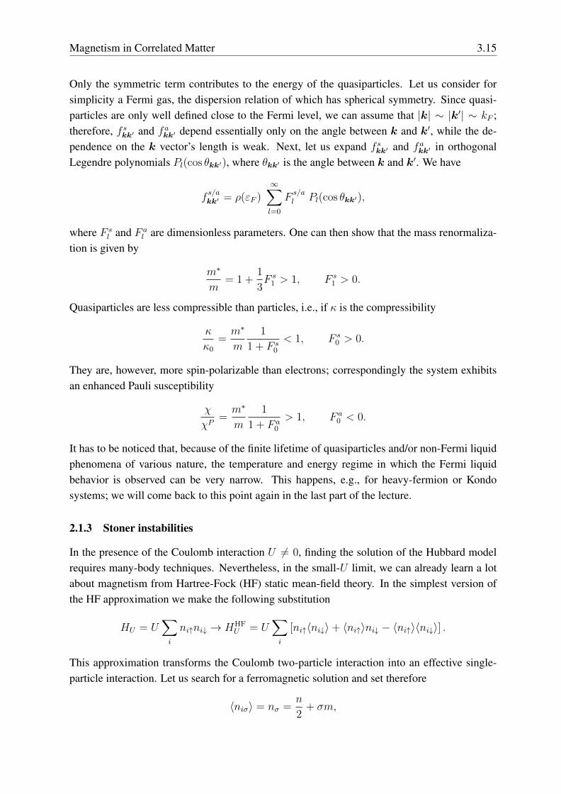
Fig. 5: Top: Effect of r = t′/t on the band structure of the two-dimensional tight-bindingmodel. Black line: Fermi level at half filling. Bottom: corresponding density of states per spin.
where m = (n↑ − n↓)/2 and n = n↑ + n↓. It is convenient to rewrite the mean-field Coulombenergy as in (10), i.e., as a function of m, n and Siz
HHFU = U
∑i
[−2mSiz +m2 +
n2
4
]. (13)
The solution of the problem defined by the HamiltonianH0+HHFU amounts to the self-consistent
solution of a non-interacting electron system with Bloch energies
εUkσ = εk + n−σ U = εk +n
2U − σmU .
In a magnetic field we additionally have to consider the Zeeman splitting. Thus
εkσ = εUkσ +1
2gµBhzσ .
In the small-U limit and for T → 0 the magnetization Mz = −gµBm is then given by
Mz ∼ χP (0)
[hz −
2
gµBUm
]= χP (0)
[hz + 2(gµB)
−2UMz
].
Solving for Mz we find the Stoner expression
χS(0; 0) =χP (0)
1− 2 (gµB)−2 UχP (0)
.
Magnetism in Correlated Matter 3.17
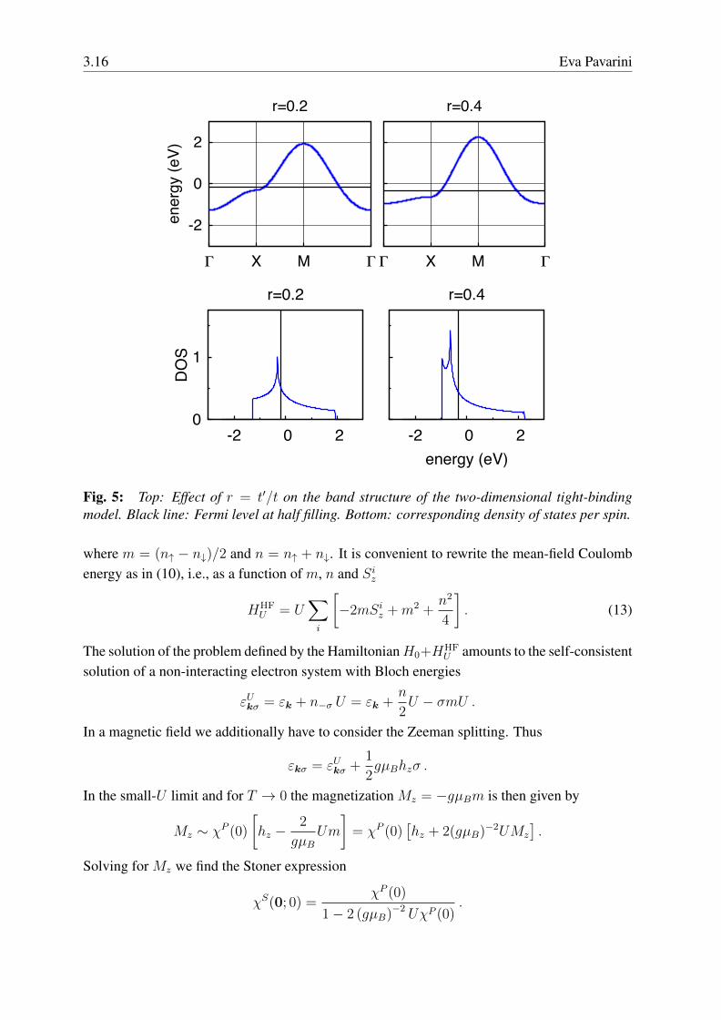
Fig. 6: Doubling of the cell due to antiferromagnetic order and the corresponding foldingof the Brillouin zone (BZ) for a two-dimensional hypercubic lattice. The antiferromagneticQ2 = (π/a, π/a, 0) vector is also shown.
Thus with increasing U the q = 0 static susceptibility increases and at the critical value
Uc = 2/ρ(εF )
diverges, i.e., even an infinitesimal magnetic field can produce a finite magnetization. Thismeans that the ground state becomes unstable against ferromagnetic order.Let us consider the case of the half-filled d-dimensional hypercubic lattice whose density ofstates is shown in Fig. 3. In three dimensions the DOS is flat around the Fermi level, e.g.,ρ(εF ) ∼ 2/W where W is the band width. For a flat DOS ferromagnetic instabilities are likelyonly when U ∼ W , a rather large value of U , which typically also brings in strong-correlationeffects not described by static mean-field theory. In two dimensions we have a rather differentsituation because a logarithmic Van-Hove singularity is exactly at the Fermi level (Fig. 3); asystem with such a density of states is unstable towards ferromagnetism even for very small U .In real materials distortions or long-range interactions typically push the Van-Hove singularitiesaway from the Fermi level. In HTSCs the electronic dispersion is modified as follows by thehopping t′ between second-nearest neighbors
εk = −2t[cos(kxa) + cos(kya)] + 4t′ cos(kxa) cos(kya) .
As shown in Fig. 4, the parameter r ∼ t′/t ranges typically from ∼ 0.15 to 0.4 [29]. Fig. 5shows that with increasing r the Van-Hove singularity moves downwards in energy.It is at this point natural to ask ourselves if ferromagnetism is the only possible instability.For a given system, magnetic instabilities with q 6= 0 might be energetically favorable com-pared to ferromagnetism; an example of a finite-q instability is antiferromagnetism (see Fig. 6).To investigate finite-q instabilities we generalize the Stoner criterion. Let us consider a mag-netic excitation characterized by the vector q commensurate with the reciprocal lattice. Thismagnetic superstructure defines a new lattice; the associated supercell includes j = 1, . . . , Nj
3.18 Eva Pavarini
d=1
X
M 0
2
40(q;0)
d=2
X
M 0
2
4d=3
X
M 0
2
4
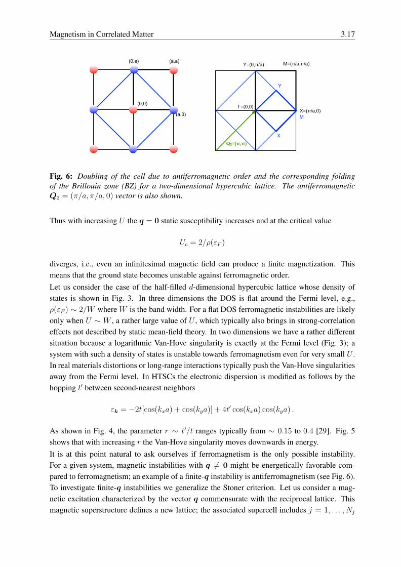
Fig. 7: The ratio χ0(q; 0)/χ0(0; 0) in the xy plane for a hypercubic lattice with t = 0.4 eV(T ∼ 230 K) at half filling. From left to right: one, two, and three dimensions.
magnetically inequivalent sites. We therefore define the quantities
Siz(q) =∑j
eiq·RjSjiz ,
〈Sjiz 〉 = m cos(q ·Rj),
where j runs over the magnetically inequivalent sites {Rj} and i over the supercells in thelattice. In the presence of a magnetic field oscillating with vector q and pointing in the zdirection, hj = hz cos(q ·Rj)z, the mean-field Coulomb and Zeeman terms can be written as
HHFU +HZ =
∑i
[gµB2
(hz −
2
gµBmU
)[Siz(q) + Siz(−q)
]+m2 +
n2
4
],
where m has to be determined self-consistently. This leads to the generalized Stoner formula
χS(q; 0) =1
2(gµB)
2 χ0(q; 0)
[1− Uχ0(q; 0)], (14)
χ0(q; 0) = −1
Nk
∑k
nk+q − nkεk+q − εk
.
Expression (14) is also known as the RPA (acronym for random-phase approximation) suscep-tibility. For q = 0 in the T → 0 limit we recover the ferromagnetic RPA susceptibility with
χ0(0; 0) = 2 (gµB)−2 χP (0) ∼ 1
2ρ(εF ) .
Figure 7 shows the non-interacting susceptibility in the xy plane for our d-dimensional hy-
Magnetism in Correlated Matter 3.19
r≈0.2
χ0(q;0)
Γ X
M 0
2
4r≈0.4
Γ X
M 0
2
4
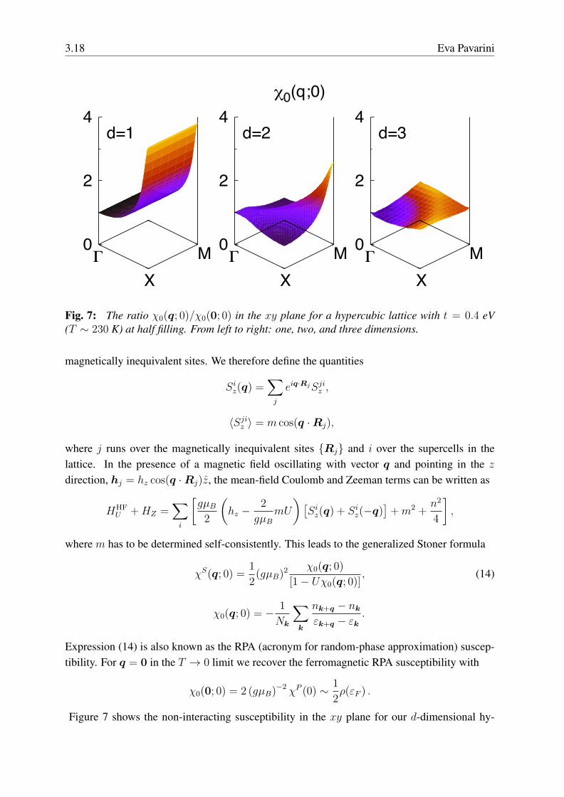
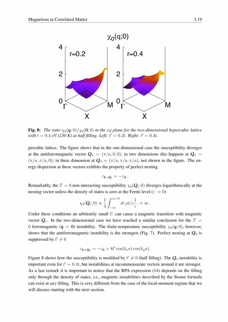
Fig. 8: The ratio χ0(q; 0)/χ0(0; 0) in the xy plane for the two-dimensional hypercubic latticewith t = 0.4 eV (230 K) at half filling. Left: t′ = 0.2t. Right: t′ = 0.4t.
percubic lattice. The figure shows that in the one-dimensional case the susceptibility divergesat the antiferromagnetic vector Q1 = (π/a, 0, 0); in two dimensions this happens at Q2 =
(π/a, π/a, 0); in three dimension at Q3 = (π/a, π/a, π/a), not shown in the figure. The en-ergy dispersion at these vectors exhibits the property of perfect nesting
εk+Qi = −εk .
Remarkably, the T = 0 non-interacting susceptibility χ0(Qi; 0) diverges logarithmically at thenesting vector unless the density of states is zero at the Fermi level (ε→ 0)
χ0(Qi; 0) ∝1
4
∫ εF=0
−∞dε ρ(ε)
1
ε→∞ .
Under these conditions an arbitrarily small U can cause a magnetic transition with magneticvector Qi. In the two-dimensional case we have reached a similar conclusion for the T =
0 ferromagnetic (q = 0) instability. The finite-temperature susceptibility χ0(q; 0), however,shows that the antiferromagnetic instability is the strongest (Fig. 7). Perfect nesting at Q2 issuppressed by t′ 6= 0
εk+Q2 = −εk + 8t′ cos(kxa) cos(kya).
Figure 8 shows how the susceptibility is modified by t′ 6= 0 (half filling). The Q2 instability isimportant even for t′ ∼ 0.4t, but instabilities at incommensurate vectors around it are stronger.As a last remark it is important to notice that the RPA expression (14) depends on the fillingonly through the density of states, i.e., magnetic instabilities described by the Stoner formulacan exist at any filling. This is very different from the case of the local-moment regime that wewill discuss starting with the next section.
3.20 Eva Pavarini
Ion n S L J 2S+1LJ
V4+ Ti3+ 3d1 1/2 2 3/2 2D3/2
V3+ 3d2 1 3 2 3F2
Cr3+ V2+ 3d3 3/2 3 3/2 4F3/2
Mn3+ Cr2+ 3d4 2 2 0 5D0
Fe3+ Mn2+ 3d5 5/2 0 5/2 6S5/2
Fe2+ 3d6 2 2 4 5D4
Co2+ 3d7 3/2 3 9/2 4F9/2
Ni2+ 3d8 1 3 4 3F4
Cu2+ 3d9 1/2 2 5/2 2D5/2
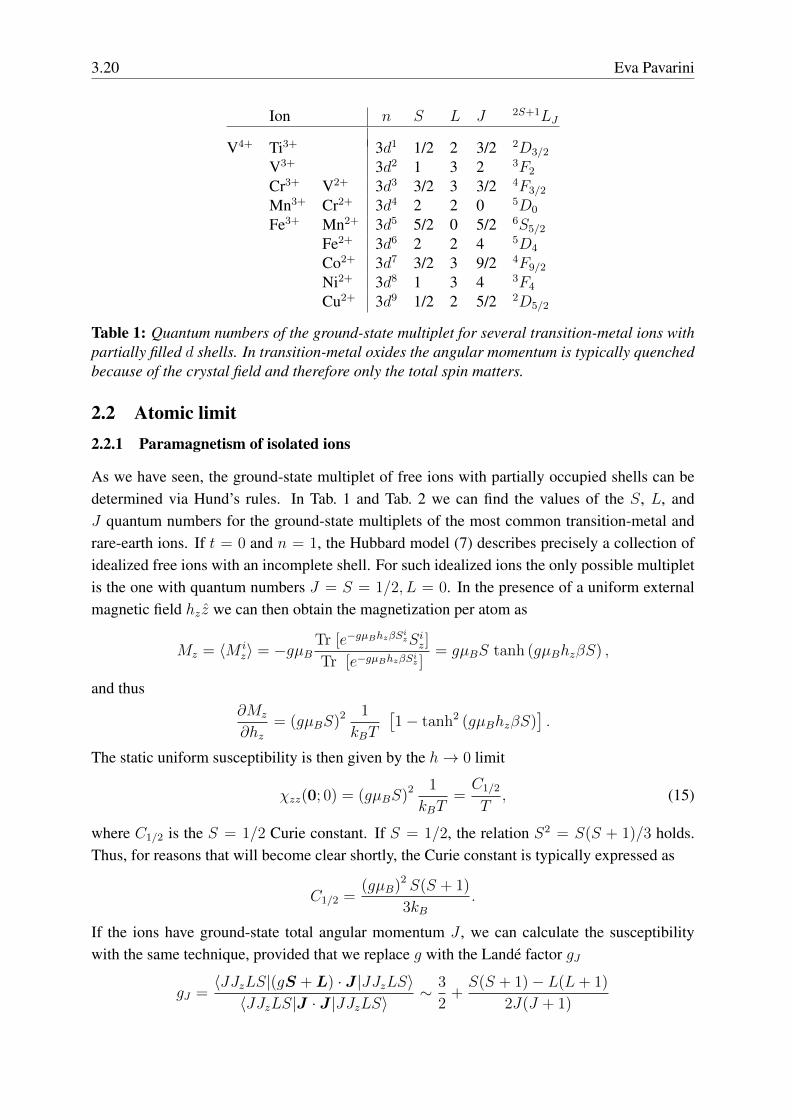
Table 1: Quantum numbers of the ground-state multiplet for several transition-metal ions withpartially filled d shells. In transition-metal oxides the angular momentum is typically quenchedbecause of the crystal field and therefore only the total spin matters.
2.2 Atomic limit2.2.1 Paramagnetism of isolated ions
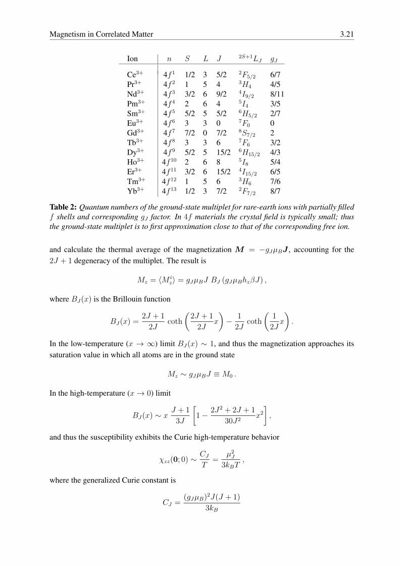
As we have seen, the ground-state multiplet of free ions with partially occupied shells can bedetermined via Hund’s rules. In Tab. 1 and Tab. 2 we can find the values of the S, L, andJ quantum numbers for the ground-state multiplets of the most common transition-metal andrare-earth ions. If t = 0 and n = 1, the Hubbard model (7) describes precisely a collection ofidealized free ions with an incomplete shell. For such idealized ions the only possible multipletis the one with quantum numbers J = S = 1/2, L = 0. In the presence of a uniform externalmagnetic field hz z we can then obtain the magnetization per atom as
Mz = 〈M iz〉 = −gµB
Tr [e−gµBhzβSizSiz]
Tr [e−gµBhzβSiz ]= gµBS tanh (gµBhzβS) ,
and thus∂Mz
∂hz= (gµBS)
2 1
kBT
[1− tanh2 (gµBhzβS)
].
The static uniform susceptibility is then given by the h→ 0 limit
χzz(0; 0) = (gµBS)2 1
kBT=C1/2
T, (15)
where C1/2 is the S = 1/2 Curie constant. If S = 1/2, the relation S2 = S(S + 1)/3 holds.Thus, for reasons that will become clear shortly, the Curie constant is typically expressed as
C1/2 =(gµB)
2 S(S + 1)
3kB.
If the ions have ground-state total angular momentum J , we can calculate the susceptibilitywith the same technique, provided that we replace g with the Lande factor gJ
gJ =〈JJzLS|(gS +L) · J |JJzLS〉〈JJzLS|J · J |JJzLS〉
∼ 3
2+S(S + 1)− L(L+ 1)
2J(J + 1)
Magnetism in Correlated Matter 3.21
Ion n S L J 2S+1LJ gJ
Ce3+ 4f 1 1/2 3 5/2 2F5/2 6/7Pr3+ 4f 2 1 5 4 3H4 4/5Nd3+ 4f 3 3/2 6 9/2 4I9/2 8/11Pm3+ 4f 4 2 6 4 5I4 3/5Sm3+ 4f 5 5/2 5 5/2 6H5/2 2/7Eu3+ 4f 6 3 3 0 7F0 0Gd3+ 4f 7 7/2 0 7/2 8S7/2 2Tb3+ 4f 8 3 3 6 7F6 3/2Dy3+ 4f 9 5/2 5 15/2 6H15/2 4/3Ho3+ 4f 10 2 6 8 5I8 5/4Er3+ 4f 11 3/2 6 15/2 4I15/2 6/5Tm3+ 4f 12 1 5 6 3H6 7/6Yb3+ 4f 13 1/2 3 7/2 2F7/2 8/7
Table 2: Quantum numbers of the ground-state multiplet for rare-earth ions with partially filledf shells and corresponding gJ factor. In 4f materials the crystal field is typically small; thusthe ground-state multiplet is to first approximation close to that of the corresponding free ion.
and calculate the thermal average of the magnetization M = −gJµBJ , accounting for the2J + 1 degeneracy of the multiplet. The result is
Mz = 〈M iz〉 = gJµBJ BJ (gJµBhzβJ) ,
where BJ(x) is the Brillouin function
BJ(x) =2J + 1
2Jcoth
(2J + 1
2Jx
)− 1
2Jcoth
(1
2Jx
).
In the low-temperature (x → ∞) limit BJ(x) ∼ 1, and thus the magnetization approaches itssaturation value in which all atoms are in the ground state
Mz ∼ gJµBJ ≡M0 .
In the high-temperature (x→ 0) limit
BJ(x) ∼ xJ + 1
3J
[1− 2J2 + 2J + 1
30J2x2
],
and thus the susceptibility exhibits the Curie high-temperature behavior
χzz(0; 0) ∼CJT
=µ2J
3kBT,
where the generalized Curie constant is
CJ =(gJµB)
2J(J + 1)
3kB
3.22 Eva Pavarini
-1
0
1
-10 -5 0 5 10
Mz/M
0
M0hz/kBT
-1
0
1
-10 -5 0 5 10
Mz/M
0
M0hz/kBT
-10
-5
0
5
10
-10 -5 0 5 10
Mz/M
0hz
M0/kBT
-10
-5
0
5
10
-10 -5 0 5 10
Mz/M
0hz
M0/kBT
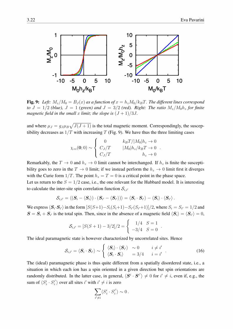
Fig. 9: Left: Mz/M0 = BJ(x) as a function of x = hzM0/kBT . The different lines correspondto J = 1/2 (blue), J = 1 (green) and J = 3/2 (red). Right: The ratio Mz/M0hz for finitemagnetic field in the small x limit; the slope is (J + 1)/3J .
and where µJ = gJµB√J(J + 1) is the total magnetic moment. Correspondingly, the suscep-
tibility decreases as 1/T with increasing T (Fig. 9). We have thus the three limiting cases
χzz(0; 0) ∼
0 kBT/|M0|hz → 0
CJ/T |M0|hz/kBT → 0
CJ/T hz → 0
.
Remarkably, the T → 0 and hz → 0 limit cannot be interchanged. If hz is finite the suscepti-bility goes to zero in the T → 0 limit; if we instead perform the hz → 0 limit first it divergeswith the Curie form 1/T . The point hz = T = 0 is a critical point in the phase space.Let us return to the S = 1/2 case, i.e., the one relevant for the Hubbard model. It is interestingto calculate the inter-site spin correlation function Si,i′
Si,i′ = 〈(Si − 〈Si〉) · (Si′ − 〈Si′〉)〉 = 〈Si · Si′〉 − 〈Si〉 · 〈Si′〉 .
We express 〈Si·Si′〉 in the form [S(S+1)−Si(Si+1)−Si′(Si′+1)]/2, where Si = Si′ = 1/2 andS = Si + Si′ is the total spin. Then, since in the absence of a magnetic field 〈Si〉 = 〈Si′〉 = 0,
Si,i′ = [S(S + 1)− 3/2]/2 =
{1/4 S = 1
−3/4 S = 0.
The ideal paramagnetic state is however characterized by uncorrelated sites. Hence
Si,i′ = 〈Si · Si′〉 ∼{〈Si〉 · 〈Si′〉 ∼ 0 i 6= i′
〈Si · Si〉 = 3/4 i = i′. (16)
The (ideal) paramagnetic phase is thus quite different from a spatially disordered state, i.e., asituation in which each ion has a spin oriented in a given direction but spin orientations arerandomly distributed. In the latter case, in general, 〈Si · Si′〉 6= 0 for i′ 6= i, even if, e.g., thesum of 〈Siz · Si
′z 〉 over all sites i′ with i′ 6= i is zero∑
i′ 6=i
〈Siz · Si′
z 〉 ∼ 0 .
Magnetism in Correlated Matter 3.23
The high-temperature static susceptibility can be obtained from the correlation function Eq. (16)using the fluctuation-dissipation theorem and the Kramers-Kronig relations (see Appendix).The result is
χzz(q; 0) ∼(gµB)
2
kBT
∑j
S i,i+jzz eiq·(Ri−Ri+j) = χizz(T ) =M2
0
kBT=C1/2
T. (17)
This shows that χzz(q; 0) is q-independent and coincides with the local susceptibility χizz(T )
χzz(0; 0) = limhz→0
∂Mz
∂hz= χizz(T ) .
How can the spin susceptibility (17) be obtained directly from Hamiltonian (10), the atomiclimit of the Hubbard model? To calculate it we can use, e.g., the imaginary-time and Matsubara-frequency formalism (see Appendix). Alternatively at high temperatures we can obtain it fromthe correlation function as we have just seen. The energies of the four atomic states are givenby (9) and, at half filling, the chemical potential is µ = εd + U/2. Therefore
χzz(0; 0) ∼(gµB)
2
kBT
Tr[e−β(Hi−µNi) (Siz)
2]
Tr [e−β(Hi−µNi)]−[Tr[e−β(Hi−µNi) Siz
]Tr [e−β(Hi−µNi)]
]2 =
C1/2
T
eβU/2
1 + eβU/2.
Thus, the susceptibility depends on the energy scale
U = E(Ni + 1) + E(Ni − 1)− 2E(Ni).
If we perform the limit U → ∞, we effectively eliminate doubly occupied and empty states.In this limit, we recover the expression that we found for the spin S = 1/2 model, Eq. (17).This is a trivial example of downfolding, in which the low-energy and high-energy sector aredecoupled in the Hamiltonian from the start. In the large-U limit the high-energy states areintegrated out leaving the system in a magnetic S = 1/2 state.
2.2.2 Larmor diamagnetism and Van Vleck paramagnetism
For ions with J = 0 the ground-state multiplet, in short |0〉, is non-degenerate and the lin-ear correction to the ground-state total energy due to the Zeeman term is zero. Remarkably,for open-shell ions the magnetization nevertheless remains finite because of higher-order cor-rections. At second order there are two contributions for the ground state. The first is theVan-Vleck term
MVVz = 2hzµ
2B
∑I
|〈0|(Lz + gSz)|I〉|2EI − E0
,
where EI is the energy of the excited state |I〉 and E0 the energy of the ground-state multiplet.The Van Vleck term is weakly temperature-dependent and typically small. The second term isthe diamagnetic Larmor contribution
MLz = −1
4hz〈0|
∑i
(x2i + y2
i )|0〉.
The Larmor and Van Vleck terms have opposite signs and typically compete with each other.
3.24 Eva Pavarini
2.3 Strong-correlation limit2.3.1 From the Hubbard model to the Heisenberg model
In the large-U limit and at half filling we can map the Hubbard model onto an effective Heisen-berg model. In this section we solve the latter using static mean-field theory. In the mean-fieldapproximation we replace the Heisenberg Hamiltonian (11) with
HMFS =
1
2Γ∑〈ii′〉
[Si · 〈Si′〉+ 〈Si〉 · Si′ − 〈Si〉 · 〈Si′〉 −
1
4nini′
].
In the presence of an external magnetic field h we add the Zeeman term and have in total
H = gµB∑i
[Si · (h+ hmi ) + const.] ,
hmi = n〈ii′〉Γ 〈Si′〉/gµB ,
where n〈ii′〉 is the number of first nearest neighbors and hmi is the molecular field at site i.We define the quantization axis z as the direction of the external magnetic field, h = hz z,and assume that z is also the direction of the molecular field, hmi = ∆hiz z. Since Γ > 0 andhypercubic lattices are bipartite, the likely magnetic order is two-sublattice antiferromagnetism.Thus we set MA
z = −gµB〈Siz〉, MBz = −gµB〈Si′z 〉, where A and B are the two sublattices,
i ∈ A and i′ ∈ B. In the absence of an external magnetic field, the total magnetization performula unit, Mz = (MB
z +MAz )/2, vanishes in the antiferromagnetic state (MB
z = −MAz ).
We define therefore as the order parameter σm = 2m = (MBz −MA
z )/2M0, which is zero onlyabove the critical temperature for antiferromagnetic order. We then calculate the magnetizationfor each sublattice and find the system of coupled equations{
MAz /M0 = B1/2
[M0(hz +∆hAz )β
]MB
z /M0 = B1/2
[M0(hz +∆hBz )β
] , (18)
where {∆hAz = −(MB
z /M0)S2Γn〈ii′〉/M0
∆hBz = −(MAz /M0)S
2Γn〈ii′〉/M0
.
For hz = 0 the system (18) can be reduced to the single equation
σm = B1/2
[σmS
2Γn〈ii′〉β]. (19)
This equation always has the trivial solution σm = 0. Figure 10 shows that, for small-enoughtemperatures it also has a non-trivial solution σm 6= 0. The order parameter σm equals ±1 atzero temperature, and its absolute value decreases with increasing temperature. It becomes zerofor T ≥ TN with
kBTN =S(S + 1)
3n〈ii′〉Γ.
Magnetism in Correlated Matter 3.25
0
1
0 0.5 1 1.5 2
σm
x
T>TN T=TN
T<TN
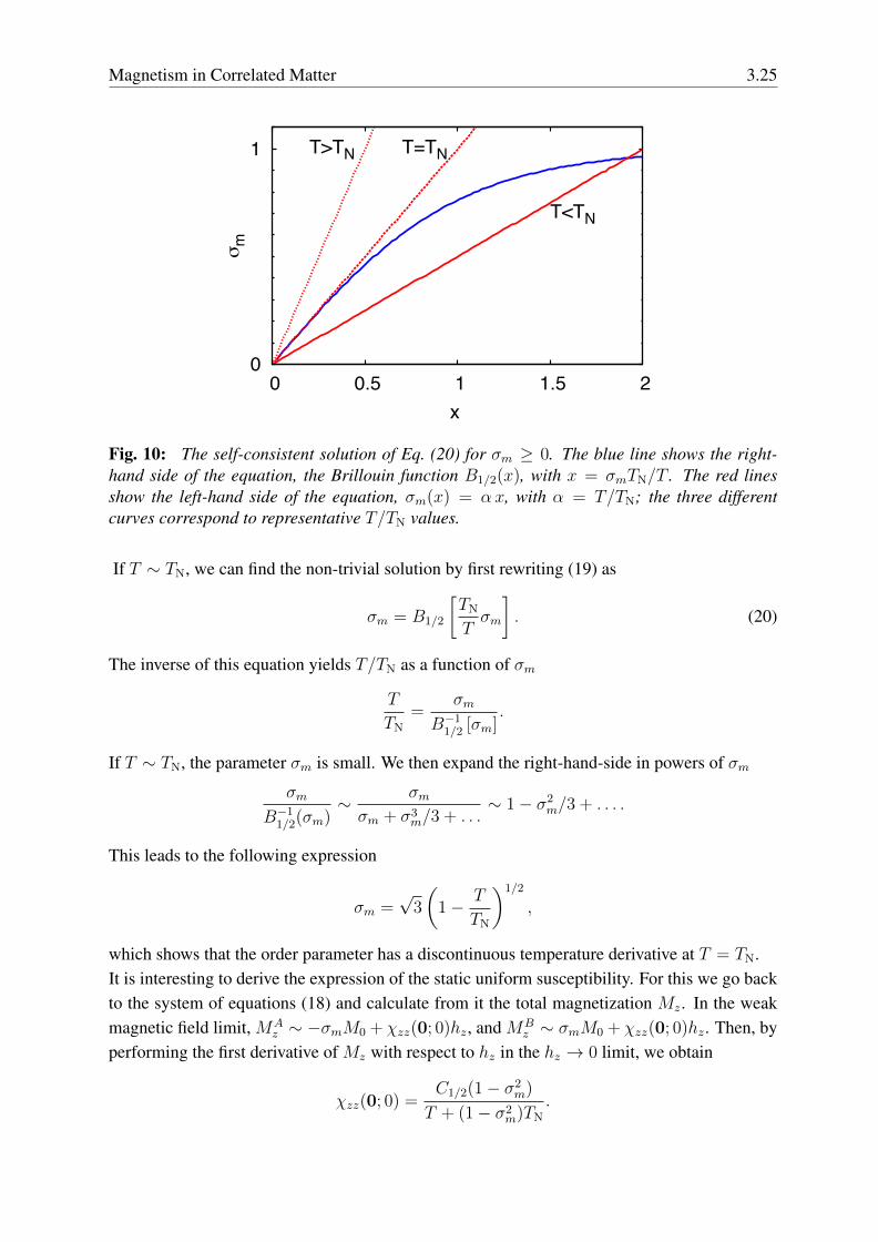
Fig. 10: The self-consistent solution of Eq. (20) for σm ≥ 0. The blue line shows the right-hand side of the equation, the Brillouin function B1/2(x), with x = σmTN/T . The red linesshow the left-hand side of the equation, σm(x) = αx, with α = T/TN; the three differentcurves correspond to representative T/TN values.
If T ∼ TN, we can find the non-trivial solution by first rewriting (19) as
σm = B1/2
[TN
Tσm
]. (20)
The inverse of this equation yields T/TN as a function of σm
T
TN
=σm
B−11/2 [σm]
.
If T ∼ TN, the parameter σm is small. We then expand the right-hand-side in powers of σm
σm
B−11/2(σm)
∼ σmσm + σ3
m/3 + . . .∼ 1− σ2
m/3 + . . . .
This leads to the following expression
σm =√3
(1− T
TN
)1/2
,
which shows that the order parameter has a discontinuous temperature derivative at T = TN.It is interesting to derive the expression of the static uniform susceptibility. For this we go backto the system of equations (18) and calculate from it the total magnetization Mz. In the weakmagnetic field limit, MA
z ∼ −σmM0 + χzz(0; 0)hz, and MBz ∼ σmM0 + χzz(0; 0)hz. Then, by
performing the first derivative of Mz with respect to hz in the hz → 0 limit, we obtain
χzz(0; 0) =C1/2(1− σ2
m)
T + (1− σ2m)TN
.
3.26 Eva Pavarini
The uniform susceptibility vanishes at T = 0 and reaches the maximum at T = TN, where ittakes the value C1/2/2TN. In the high-temperature regime σm = 0 and
χzz(0; 0) ∼C1/2
T + TN
,
which is smaller than the susceptibility of free S = 1/2 magnetic ions.The magnetic linear response is quite different if we apply an external field h⊥ perpendicularto the spins in the antiferromagnetic lattice. The associated perpendicular magnetization is
M⊥ ∼M0σm(gµBh⊥)√
(gµBh⊥)2 + (4σm)2(kBTN)2,
and therefore the perpendicular susceptibility is temperature-independent for T ≤ TN
χ⊥(0; 0) = limh⊥→0
dM⊥dh⊥
=C1/2
2TN
.
Hence, for T < TN the susceptibility is anisotropic, χzz(0; 0) = χ‖(0; 0) 6= χ⊥(0; 0); atabsolute zero χ‖(0; 0) vanishes, but the response to h⊥ remains strong. For T > TN the orderparameter is zero and the susceptibility isotropic, χ‖(0; 0) = χ⊥(0; 0).We have up to now considered antiferromagnetic order only. What about other magnetic insta-bilities? Let us consider first ferromagnetic order. For a ferromagnetic spin arrangement, byrepeating the calculation, we find
χzz(0; 0) =C1/2(1− σ2
m)
T − (1− σ2m)TC
,
where TC = −S(S + 1)n〈ii′〉Γ/3kB is, if the exchange coupling Γ is negative, the criticaltemperature for ferromagnetic order. Then, in contrast to the antiferromagnetic case, the high-temperature uniform susceptibility is larger than that of free S = 1/2 magnetic ions.For a generic magnetic structure characterized by a vector q and a supercell with j = 1, . . . , Nj
magnetically inequivalent sites we make the ansatz
〈M jiz 〉 = −σmM0 cos(q ·Rj) = −gµBm cos(q ·Rj) ,
where σm is again the order parameter, i identifies the supercell, andRj the position of the j-thinequivalent site. We consider a magnetic field rotating with the same q vector. By using thestatic mean-field approach we then find
kBTq =S(S + 1)
3Γq, Γq = −
∑ij 6=0
Γ 00,ijeiq·(Ti+Rj), (21)
where Γ 00,ij is the exchange coupling between the spin at the origin and the spin at site Ti+Rj
(ij in short); {Rj} are vectors inside a supercell and {Ti} are lattice vectors. In our example,T0 = TC and TqAF
= TN = −TC. Thus we have
χzz(q; 0) =C1/2(1− σ2
m)
T − (1− σ2m)Tq
, (22)
Magnetism in Correlated Matter 3.27
which diverges at T = Tq. The susceptibility χzz(q; 0) reflects the spatial extent of correlations,i.e., the correlation length ξ; the divergence of the susceptibility at Tq is closely related to thedivergence of ξ. To see this we calculate ξ for a hypercubic three-dimensional lattice, assumingthat the system has only one instability with vector Q. First we expand Eq. (21) around Qobtaining Tq ∼ TQ + α(q −Q)2 + . . . , and then we calculate χ00,ji
zz , the Fourier transform ofEq. (22). We find that χ00,ji
zz decays exponentially with r = |Ti + Rj|, i.e., χ00,jizz ∝ e−r/ξ/r.
The range of the correlations is ξ ∝ [TQ/(T − TQ)]1/2, which becomes infinite at T = TQ.It is important to notice that in principle there can be instabilities at any q vector, i.e., q neednot be commensurate with reciprocal lattice vectors. The value of q for which Tq is the largestdetermines (within static mean-field theory) the type of magnetic order that is realized. Theantiferromagnetic structure in Fig. 6 corresponds to qAF = Q2 = (π/a, π/a, 0).In real systems the spin S is typically replaced by an effective magnetic moment, µeff , andtherefore C1/2 → Ceff = µ2
eff/3kB. It follows that µeff is the value of the product 3kBTχzz(q; 0)in the high-temperature limit (here T � Tq). The actual value of µeff depends, as we havediscussed in the introduction, on the Coulomb interaction, the spin-orbit coupling and the crystalfield. In addition, the effective moment can be screened by many-body effects, as happens forKondo impurities; we will discuss the latter case in the last section.
2.3.2 The Hartree-Fock approximation
We have seen that Hartree-Fock (HF) mean-field theory yields Stoner magnetic instabilities inthe weak-coupling limit. Can it also describe magnetism in the local-moment regime (t/U �1)? Let us focus on the half-filled two-dimensional Hubbard model for a square lattice, and letus analyze two possible magnetically ordered states, the ferro- and the antiferromagnetic state.If we are only interested in the ferromagnetic or the paramagnetic solution, the HF approxima-tion of the Coulomb term in the Hubbard model is given by Eq. (13). Thus the Hamiltonian isH = Hd + HT + HHF
U with HHFU = U
∑i[−2mSiz + m2 + 1
4n2]. For periodic systems it is
convenient to write H in k space. We then adopt as one-electron basis the Bloch states
Ψkσ(r) =1√Ns
∑i
eik·Ti Ψiσ(r),
where Ψiσ(r) is a Wannier function with spin σ, Ti a lattice vector, and Ns the number of latticesites. The term HHF
U depends on the spin operator Siz, which can be written in k space as
Siz =1
Nk
∑kk′
ei(k−k′)·Ti 1
2
∑σ
σc†kσck′σ︸ ︷︷ ︸Sz(k,k′)
=1
Nk
∑kk′
ei(k−k′)·TiSz(k,k
′).
The term HHFU has the same periodicity as the lattice and does not couple states with different
k vectors. Thus only Sz(k,k) contributes, and the Hamiltonian can be written as
H =∑σ
∑k
εknkσ + U∑k
[−2m Sz(k,k) +m2 +
n2
4
]︸ ︷︷ ︸
HHFU = U
∑i[−2mSiz +m2 + 1
4n2]
,
3.28 Eva Pavarini
-2
0
2
Γ X M Γ
ener
gy (e
V)mU=0
Γ X M Γ
mU=2t
Γ X M Γ
mU=2t
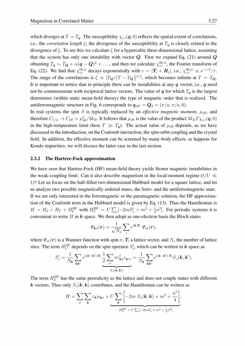
Fig. 11: Ferromagnetism in Hartree-Fock. The chemical potential is taken as the energy zero.
where m = (n↑ − n↓)/2 and n = 1; for simplicity we set εd = 0. The HF correction splits thebands with opposite spin, leading to new one-electron eigenvalues, εkσ = εk+
12U − σUm; the
chemical potential is µ = U/2. The separation between εk↑ − µ and εk↓ − µ is 2mU , as canbe seen in Fig. 11. The system remains metallic for U smaller than the bandwidth W . In thesmall-t/U limit and at half filling we can assume that the system is a ferromagnetic insulatorand m = 1/2. The total energy of the ground state is then
EF =1
Nk
∑k
[εkσ − µ] =1
Nk
∑k
[εk −
1
2U
]= −1
2U.
Let us now describe the same periodic lattice via a supercell which allows for a two-sublatticeantiferromagnetic solution; this supercell is shown in Fig. 6. We rewrite the Bloch states of theoriginal lattice as
Ψkσ(r) =1√2
[ΨAkσ(r) + ΨBkσ(r)
], Ψαkσ(r) =
1√Nsα
∑iα
eiTαi ·k Ψiασ(r).
Here A and B are the two sublattices with opposite spins and T Ai and TB
i are their lattice vec-tors; α = A,B. We take as one-electron basis the two Bloch functions Ψkσ and Ψk+Q2σ, whereQ2 = (π/a, π/a, 0) is the vector associated with the antiferromagnetic instability and the cor-responding folding of the Brillouin zone, also shown in Fig. 6. Then, in the HF approximation,the Coulomb interaction is given by
HHFU =
∑i∈A
[−2mSiz +m2 +
n2
4
]+∑i∈B
[+2mSiz +m2 +
n2
4
].
This interaction couples Bloch states with k vectors made equivalent by the folding of theBrillouin zone. Thus the HF Hamiltonian takes the form
H =∑k
∑σ
εknkσ +∑k
∑σ
εk+Q2nk+Q2σ + U∑k
[−2m Sz(k,k +Q2) + 2m2 + 2
n2
4
]︸ ︷︷ ︸
static mean-field correction HHFU
.
Magnetism in Correlated Matter 3.29
-2
0
2
Γ X M Γ
ener
gy (e
V)mU=0
-2
0
2
Γ X M Γ
ener
gy (e
V)mU=0
Γ X M Γ
mU=0.5t
Γ X M Γ
mU=0.5t
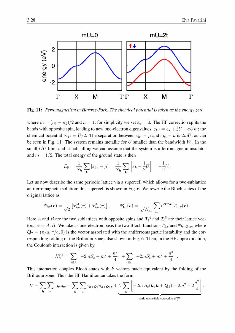
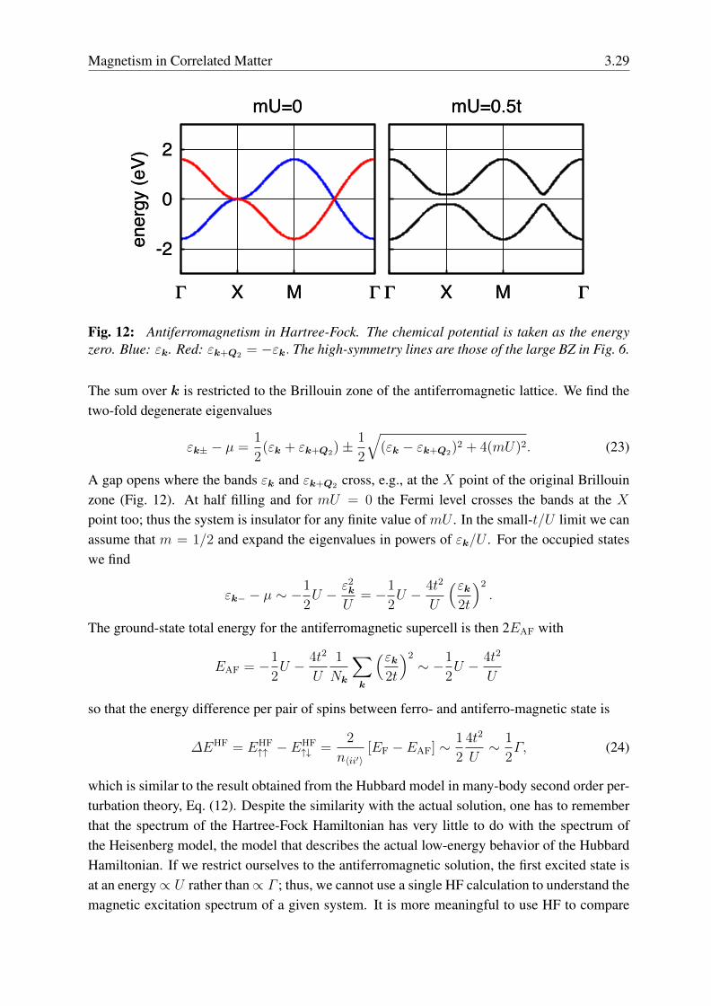
Fig. 12: Antiferromagnetism in Hartree-Fock. The chemical potential is taken as the energyzero. Blue: εk. Red: εk+Q2 = −εk. The high-symmetry lines are those of the large BZ in Fig. 6.
The sum over k is restricted to the Brillouin zone of the antiferromagnetic lattice. We find thetwo-fold degenerate eigenvalues
εk± − µ =1
2(εk + εk+Q2)±
1
2
√(εk − εk+Q2)
2 + 4(mU)2. (23)
A gap opens where the bands εk and εk+Q2 cross, e.g., at the X point of the original Brillouinzone (Fig. 12). At half filling and for mU = 0 the Fermi level crosses the bands at the Xpoint too; thus the system is insulator for any finite value of mU . In the small-t/U limit we canassume that m = 1/2 and expand the eigenvalues in powers of εk/U . For the occupied stateswe find
εk− − µ ∼ −1
2U − ε2
k
U= −1
2U − 4t2
U
(εk2t
)2
.
The ground-state total energy for the antiferromagnetic supercell is then 2EAF with
EAF = −1
2U − 4t2
U
1
Nk
∑k
(εk2t
)2
∼ −1
2U − 4t2
U
so that the energy difference per pair of spins between ferro- and antiferro-magnetic state is
∆EHF = EHF↑↑ − EHF
↑↓ =2
n〈ii′〉[EF − EAF] ∼
1
2
4t2
U∼ 1
2Γ, (24)
which is similar to the result obtained from the Hubbard model in many-body second order per-turbation theory, Eq. (12). Despite the similarity with the actual solution, one has to rememberthat the spectrum of the Hartree-Fock Hamiltonian has very little to do with the spectrum ofthe Heisenberg model, the model that describes the actual low-energy behavior of the HubbardHamiltonian. If we restrict ourselves to the antiferromagnetic solution, the first excited state isat an energy∝ U rather than∝ Γ ; thus, we cannot use a single HF calculation to understand themagnetic excitation spectrum of a given system. It is more meaningful to use HF to compare
3.30 Eva Pavarini
the total energy of different states and determine in this way, within HF, the ground state. Evenin this case, however, one has to keep in mind that HF suffers from spin contamination, i.e.,singlet states and Sz = 0 triplet states mix [26]. The energy difference per bond EHF
↑↑ − EHF↑↓
in Eq. (24) only resembles the exact result, as one can grasp by comparing it with the actualenergy difference between triplet and singlet state in the two-site Heisenberg model
∆E = ES=1 − ES=0 = Γ,
which is a factor of two larger. The actual ratio ∆E/∆EHF might depend on the details ofthe HF band structures. Thus, overall, Hartree-Fock is not the ideal approach to determine theonset of magnetic phase transitions. Other shortcomings of the Hartree-Fock approximation arein the description of the Mott metal-insulator transition. In Hartree-Fock the metal-insulatortransition is intimately related to long-range magnetic order (Slater transition), but in stronglycorrelated materials the metal-insulator transition can occur in the paramagnetic phase (Motttransition). It is associated with a divergence of the self-energy at low frequencies rather thanwith the formation of superstructures. This physics, captured by many-body methods such asthe dynamical mean-field theory [15], is completely missed by the Hartree-Fock approximation.
2.3.3 The dynamical mean-field theory approach
The modern approach for solving the Hubbard model is the so-called dynamical mean-field the-ory method [14–16]. In DMFT the lattice Hubbard model is mapped onto a self-consistent quan-tum impurity model describing an impurity coupled to a non-correlated conduction-electronbath. The quantum impurity model is typically the Anderson model, which will be discussedin detail in the next chapter. Here we do not want to focus on the specific form of the quantumimpurity model but rather on the core aspects of the DMFT approach and on the comparison ofDMFT with Hartree-Fock. In Hartree-Fock the effective mean field is an energy-independent(static) parameter; in the example discussed in the previous section it is a function of the mag-netic order parameter m. In DMFT the role of the effective mean-field is played by the bathGreen functionG0(iνn) where νn is a fermionic Matsubara frequency; it is frequency dependent(dynamical) and related to the impurity Green function G(iνn) via the Dyson equation
[G(iνn)]−1 = [G0(iνn)]
−1 −Σ(iνn) , (25)
where Σ(iνn) is the impurity self-energy. As in any mean-field theory, the effective field isdetermined by enforcing a self-consistency condition. In DMFT the latter requires that theimpurity Green function G(iνn), calculated by solving the quantum impurity model, equalsGii(iνn), the lattice Green function at a site i
Gii(iνn) = G(iνn),
with
Gii(iνn) =1
Nk
∑k
G(k; iνn) =1
Nk
∑k
1
iνn − εk −Σ(iνn) + µ.
Magnetism in Correlated Matter 3.31
E
Hartree-Fock DMFT
Ti
⌃0"(!)
⌃0#(!)
!
!
Ti+1Ti�1
⌃0i"
⌃0i#
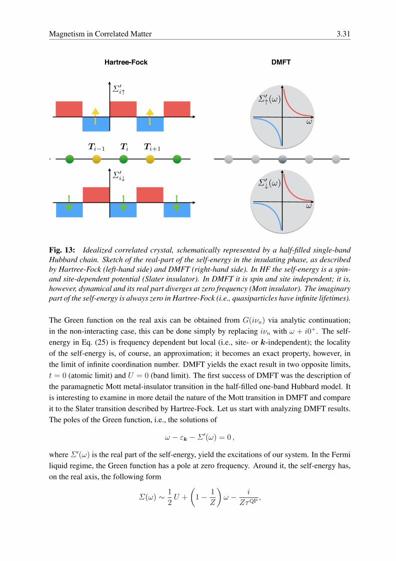
Fig. 13: Idealized correlated crystal, schematically represented by a half-filled single-bandHubbard chain. Sketch of the real-part of the self-energy in the insulating phase, as describedby Hartree-Fock (left-hand side) and DMFT (right-hand side). In HF the self-energy is a spin-and site-dependent potential (Slater insulator). In DMFT it is spin and site independent; it is,however, dynamical and its real part diverges at zero frequency (Mott insulator). The imaginarypart of the self-energy is always zero in Hartree-Fock (i.e., quasiparticles have infinite lifetimes).
The Green function on the real axis can be obtained from G(iνn) via analytic continuation;in the non-interacting case, this can be done simply by replacing iνn with ω + i0+. The self-energy in Eq. (25) is frequency dependent but local (i.e., site- or k-independent); the localityof the self-energy is, of course, an approximation; it becomes an exact property, however, inthe limit of infinite coordination number. DMFT yields the exact result in two opposite limits,t = 0 (atomic limit) and U = 0 (band limit). The first success of DMFT was the description ofthe paramagnetic Mott metal-insulator transition in the half-filled one-band Hubbard model. Itis interesting to examine in more detail the nature of the Mott transition in DMFT and compareit to the Slater transition described by Hartree-Fock. Let us start with analyzing DMFT results.The poles of the Green function, i.e., the solutions of
ω − εk −Σ ′(ω) = 0 ,
where Σ ′(ω) is the real part of the self-energy, yield the excitations of our system. In the Fermiliquid regime, the Green function has a pole at zero frequency. Around it, the self-energy has,on the real axis, the following form
Σ(ω) ∼ 1
2U +
(1− 1
Z
)ω − i
ZτQP,
3.32 Eva Pavarini
where the positive dimensionless number Z yields the mass enhancement, m∗/m ∼ 1/Z, andthe positive parameter τQP ∼ 1/(aT 2 + bω2) is the quasiparticles lifetime; at higher frequencythe self-energy yields two additional poles corresponding to the Hubbard bands. In the Mottinsulating regime the central quasiparticle peak disappears, and only the Hubbard bands remain.The self-energy has approximately the form
Σ(ω) ∼ rU2
4
[1
ω− iπδ(ω)− ifU(ω)
],
where fU(ω) is a positive function that is zero inside the gap and r is a model-specific renormal-ization factor. Hence, the real-part of the self-energy diverges at zero frequency, and there areno well defined low-energy quasiparticles. Furthermore, since we are assuming that the systemis paramagnetic, the self-energy and the Green function are independent of the spin
Σσ(ω) = Σ(ω)
Gσ(ω) = G(ω)
Gσ(k;ω) = G(k;ω).
Thus DMFT can be seen, to some extent, as a complementary approximation to Hartree-Fock.If we write the Hartree-Fock correction to the energies in the form of a self-energy, the latter isa real, static but spin- and site-dependent potential. More specifically, we have at site i
ΣHFiσ (ω) = U
[ni−σ −
1
2
],
where niσ is the site occupation for spin σ. Let us consider the antiferromagnetic case. For this,as we have seen, we have to consider two sublattices or a two-site cluster; the magnetization atsites j, nearest neighbors of site i, has opposite sign than at site i. Thus
ΣHFjσ (ω) = −U
[ni−σ −
1
2
].
This spatial structure of the self-energy is what opens the gap shown in Fig. 12; this picture ofthe gap opening is very different from the one emerging from DMFT; as we have just seen, inDMFT the gap opens via the divergence at zero frequency in the real-part of the self-energy;this happens already in a single-site paramagnetic calculation, i.e., we do not have to assumeany long-range magnetic order. In HF the self-energy resulting from a non-magnetic (m = 0)single-site calculation is instead a mere energy shift – the same for all sites and spins – and doesnot change the band structure at all. Hartree-Fock is not, e.g., the large-U limit of DMFT butmerely the large frequency limit of DMFT (or of its cluster extensions). The differences amongthe two approaches are pictorially shown in Fig. 13 for an idealized one-dimensional crystal.Let us now focus on the magnetic properties of the Hubbard model, and in particular on themagnetic susceptibility χzz(q; iωm). Since in DMFT we solve the quantum impurity modelexactly, we can directly calculate the local linear-response tensor, and therefore the local sus-ceptibility χzz(iωm). If we are interested in magnetic order, however, we need also, at least
Magnetism in Correlated Matter 3.33
=
+!n
"o!nk
!n+#mk+q
k
!n+#mk+q
"!n
!n+#m !n′+#m
!n′
k+q
k
k′+q
k′
"
$ ""o!n+#mk+q
!n k!n′
k′
!n′+#mk′+q
α′
α′
α′
αα
α
γ
γ′
γ′
γγ
γ′
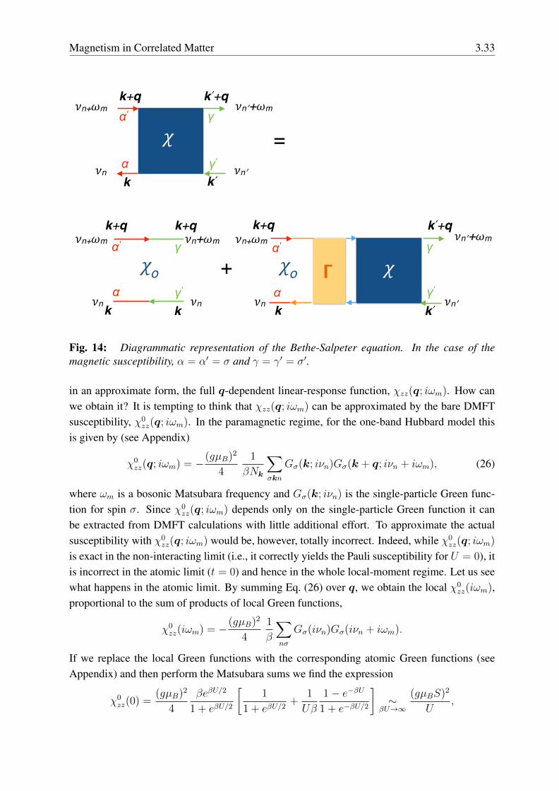
Fig. 14: Diagrammatic representation of the Bethe-Salpeter equation. In the case of themagnetic susceptibility, α = α′ = σ and γ = γ′ = σ′.
in an approximate form, the full q-dependent linear-response function, χzz(q; iωm). How canwe obtain it? It is tempting to think that χzz(q; iωm) can be approximated by the bare DMFTsusceptibility, χ0
zz(q; iωm). In the paramagnetic regime, for the one-band Hubbard model thisis given by (see Appendix)
χ0zz(q; iωm) = −
(gµB)2
4
1
βNk
∑σkn
Gσ(k; iνn)Gσ(k + q; iνn + iωm), (26)
where ωm is a bosonic Matsubara frequency and Gσ(k; iνn) is the single-particle Green func-tion for spin σ. Since χ0
zz(q; iωm) depends only on the single-particle Green function it canbe extracted from DMFT calculations with little additional effort. To approximate the actualsusceptibility with χ0
zz(q; iωm) would be, however, totally incorrect. Indeed, while χ0zz(q; iωm)
is exact in the non-interacting limit (i.e., it correctly yields the Pauli susceptibility for U = 0), itis incorrect in the atomic limit (t = 0) and hence in the whole local-moment regime. Let us seewhat happens in the atomic limit. By summing Eq. (26) over q, we obtain the local χ0
zz(iωm),proportional to the sum of products of local Green functions,
χ0zz(iωm) = −
(gµB)2
4
1
β
∑nσ
Gσ(iνn)Gσ(iνn + iωm).
If we replace the local Green functions with the corresponding atomic Green functions (seeAppendix) and then perform the Matsubara sums we find the expression
χ0zz(0) =
(gµB)2
4
βeβU/2
1 + eβU/2
[1
1 + eβU/2+
1
Uβ
1− e−βU1 + e−βU/2
]∼
βU→∞
(gµBS)2
U,
3.34 Eva Pavarini
Green Function Susceptibility
local self-energy approximation local vertex approximation
local Dyson equation local Bethe-Salpeter equation
k-dependent Dyson equation matrix q-dependent Bethe-Salpeter equation matrix
G(k; i⌫n) = G0(k; i⌫n) + G0(k; i⌫n)⌃(k; i⌫n)G(k; i⌫n)
G(i⌫n) = G0(i⌫n) + G0(i⌫n)⌃(i⌫n)G(i⌫n)
� (q; i!m) ! � (i!m)
�(q; i!m) = �0(q; i!m) + �0(q; i!m)� (q; i!m)�(q; i!m)
�(i!m) = �0(i!m) + �0(i!m)� (i!m)�(i!m)
⌃(k; i⌫n) ! ⌃(i⌫n)
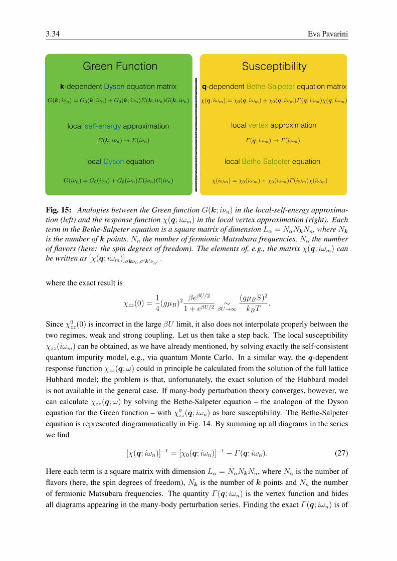
Fig. 15: Analogies between the Green function G(k; iνn) in the local-self-energy approxima-tion (left) and the response function χ(q; iωm) in the local vertex approximation (right). Eachterm in the Bethe-Salpeter equation is a square matrix of dimension Lα = NαNkNn, where Nkis the number of k points, Nn the number of fermionic Matsubara frequencies, Nα the numberof flavors (here: the spin degrees of freedom). The elements of, e.g., the matrix χ(q; iωm) canbe written as [χ(q; iωm)]σkνn,σ′k′νn′ .
where the exact result is
χzz(0) =1
4(gµB)
2 βeβU/2
1 + eβU/2∼
βU→∞
(gµBS)2
kBT.
Since χ0zz(0) is incorrect in the large βU limit, it also does not interpolate properly between the
two regimes, weak and strong coupling. Let us then take a step back. The local susceptibilityχzz(iωm) can be obtained, as we have already mentioned, by solving exactly the self-consistentquantum impurity model, e.g., via quantum Monte Carlo. In a similar way, the q-dependentresponse function χzz(q;ω) could in principle be calculated from the solution of the full latticeHubbard model; the problem is that, unfortunately, the exact solution of the Hubbard modelis not available in the general case. If many-body perturbation theory converges, however, wecan calculate χzz(q;ω) by solving the Bethe-Salpeter equation – the analogon of the Dysonequation for the Green function – with χ0
zz(q; iωn) as bare susceptibility. The Bethe-Salpeterequation is represented diagrammatically in Fig. 14. By summing up all diagrams in the serieswe find
[χ(q; iωn)]−1 = [χ0(q; iωn)]
−1 − Γ (q; iωn). (27)
Here each term is a square matrix with dimension Lα = NαNkNn, where Nα is the number offlavors (here, the spin degrees of freedom), Nk is the number of k points and Nn the numberof fermionic Matsubara frequencies. The quantity Γ (q; iωn) is the vertex function and hidesall diagrams appearing in the many-body perturbation series. Finding the exact Γ (q; iωn) is of
Magnetism in Correlated Matter 3.35
course as difficult as solving the full many-body problem; we therefore have to find a reasonableapproximation. In the spirit of DMFT, let us assume that the vertex entering the Bethe-Salpeterequation can be replaced by a local function
Γ (q; iωn)→ Γ (iωn).
Furthermore, let us assume that the local vertex solves, in turn, a local version of the Bethe-Salpeter equation
Γ (iωm) = [χ0(iωm)]−1 − [χ(iωm)]
−1. (28)
The local vertex Γ (iωm), calculated via Eq. (28), can then be used to compute the susceptibilityfrom the q-dependent Bethe-Salpeter equation Eq. (27). The analogy between the calculationof the susceptibility in the local vertex approximation and that of the Green function in the localself-energy approximation is shown in Fig. 15.Let us now qualitatively discuss the magnetic susceptibility of the one-band Hubbard model inthe Mott-insulating limit. For simplicity, let us now assume that the vertex is static and thusthat we can replace all susceptibility matrices in the Bethe-Salpeter equation with the physicalsusceptibilities, which we obtain by summing over the fermionic Matsubara frequencies andthe momenta. For the magnetic susceptibility this means
χzz(q; iωm) =(gµB)2 1
β2
1
4
∑σσ′
σσ′∑nn′
1
N2k
∑kk′
1
β[χ(q; iωm)]σkνn,σ′k′νn′
=(gµB)2
∫dτ eiωmτ 〈Sz(τ)Sz(0)〉.
In the high-temperature and large-U limit (βU →∞ and T � TN ) the static local susceptibilityis approximatively given by the static atomic susceptibility
χzz(0) ∼µ2
eff
kBT,
where µ2eff = (gµB)
2S(S + 1)/3. Therefore the vertex is roughly given by
Γ (0) ∼ 1
χ0zz(0)
− kBT
µ2eff
.
The susceptibility calculated with such a local vertex is
χzz(q; 0) ∼µ2
eff
kBT − µ2effJ(q)
≡ µ2eff
kB(T − Tq),
where the coupling is given by
J(q) = −[
1
χ0zz(q; 0)
− 1
χ0zz(0)
].
Thus, in the strong-correlation limit, the Bethe-Salpeter equation, solved assuming the vertexis local and, in addition, static, yields a static high-temperature susceptibility of Curie-Weissform. We had found the same form of the susceptibility by solving the Heisenberg model inthe static mean-field approximation. A more detailed presentation of the DMFT approach tocalculate linear-response functions can be found in Ref. [27].
3.36 Eva Pavarini
3 The Anderson model
The Kondo impurity is a representative case of a system that exhibits both local-moment andPauli-paramagnetic behavior, although in quite different temperature regimes [12]. The Kondoeffect was first observed in diluted metallic alloys, metallic systems in which isolated d or fmagnetic impurities are present, and it has been a riddle for decades. A Kondo impurity in ametallic host can be described by the Anderson model
HA =∑σ
∑k
εknkσ +∑σ
εfnfσ + Unf↑nf↓︸ ︷︷ ︸H0
+∑σ
∑k
[Vkc
†kσcfσ + h.c.
]︸ ︷︷ ︸
H1
, (29)
where εf is the impurity level (occupied by nf ∼ 1 electrons), εk is the dispersion of the metallicband, and Vk the hybridization. If we assume that the system has particle-hole symmetry withrespect to the Fermi level, then εf − µ = −U/2. The Kondo regime is characterized by theparameter values εf � µ and εf + U � µ and by a weak hybridization, i.e., the hybridizationwidth
∆(ε) = π1
Nk
∑k
|Vk|2δ(εk − ε)
is such that ∆(µ) � |µ− εf |, |µ− εf − U |. The Anderson model is also used as the quantumimpurity problem in dynamical mean-field theory. In DMFT the bath parameters εk and Vkhave, in principle, to be determined self-consistently. If quantum Monte Carlo is used to solvethe Anderson model, it is sufficient to determine the bath Green function self-consistently.
3.1 The Kondo limit
Through the Schrieffer-Wolff canonical transformation [28] one can map the Anderson modelonto the Kondo model, in which only the effective spin of the impurity enters
HK = H ′0 + ΓSf · sc(0) = H ′0 +HΓ , (30)
where
Γ ∼ −2|VkF |2[1
εf− 1
εf + U
]> 0
is the antiferromagnetic coupling arising from the hybridization, Sf the spin of the impurity(Sf = 1/2), and sc(0) is the spin-density of the conduction band at the impurity site. Forconvenience we set the Fermi energy to zero; kF is a k vector at the Fermi level. The Schrieffer-Wolff canonical transformation works as follows. We introduce the operator S that transformsthe Hamiltonian H into HS
HS = eSHe−S.
Magnetism in Correlated Matter 3.37
We search for an operator S such that the transformed Hamiltonian HS has no terms of firstorder in Vk. Let us first split the original Hamiltonian HA into two pieces: H0, the sum of allterms except the hybridization term, and H1, the hybridization term. Let us choose S linear inVk and such that
[S,H0] = −H1. (31)
From Eq. (31) one finds that the operator S is given by
S =∑kσ
[1− nf−σεk − εf
+nf−σ
εk − εf − U
]Vkc
†kσcfσ − h.c..
The transformed Hamiltonian is complicated, as can be seen from explicitly writing the seriesfor a transformation satisfying Eq. (31)
HS = H0 +1
2[S,H1] +
1
3
[S, [S,H1]
]+ . . . .
In the limit in which the hybridization strength Γ is small this series can, however, be truncatedat second order. The resulting Hamiltonian has the form HS = H0 + H2, with H2 = HΓ +
Hdir +∆H0 +Hch. The first term is the exchange interaction
HΓ =1
4
∑kk′
Γkk′
[∑σ1σ2
c†k′σ1〈σ1|σ|σ2〉ckσ2 ·∑σ3σ4
c†fσ3〈σ3|σ|σ4〉cfσ4
]
where
Γkk′ = V ∗k Vk′
[1
εk − εf+
1
εk′ − εf+
1
U + εf − εk+
1
U + εf − εk′
].
Let us assume that the coupling Γkk′ is weakly dependent on k and k′; then by setting |k| ∼ kF ,and |k′| ∼ kF we recover the antiferromagnetic contact coupling in Eq. (30).The second term is a potential-scattering interaction
Hdir =∑kk′
[Akk′ −
1
4Γkk′nf
] ∑σ
c†k′σ ckσ,
where
Akk′ =1
2V ∗k Vk′
[1
εk − εf+
1
εk′ − εf
].
This term is spin-independent, and thus does not play a relevant role in the Kondo effect. Thenext term merely modifies the H0 term
∆H0 = −∑kσ
[Akk −
1
2Γkk nf−σ
]nfσ.
3.38 Eva Pavarini
Finally, the last term is a pair-hopping interaction, which changes the charge of the f sites bytwo electrons and thus can be neglected if nf ∼ 1
∆Hch = −1
4
∑kk′σ
Γkk′c†k′−σc
†kσcfσcf−σ + h.c..
The essential term in H2 is the exchange term HΓ , which is the one that yields the antiferro-magnetic contact interaction in the Kondo Hamiltonian (30). Remarkably, the Schrieffer-Wolfftransformation generates a perturbation series in the hybridization; an analogous perturbationseries is also used in the hybridization-expansion continuous-time quantum Monte Carlo ap-proach to solve the quantum impurity problem in dynamical mean-field theory.
3.1.1 The impurity susceptibility
The solution of the problem defined by (29) or (30) is not at all trivial and requires many-bodytechniques such as the Wilson numerical renormalization group [30] or the Bethe ansatz [31].Here we only discuss some important exact results concerning the magnetic properties. Let usdefine the impurity susceptibility χfzz(T ) as the total susceptibility minus the contribution of themetallic band in the absence of the impurity [30–32]. One can show that at high temperaturesχfzz(T ) has the following behavior
χfzz(T ) ∼(gµB)
2Sf (Sf + 1)
3kBT
{1− 1
ln (T/TK)
}.
This expression resembles the Curie susceptibility, apart from the ln(T/TK) term. The scale TK
is the Kondo temperature, which, to first approximation, is given by
kBTK ∼ De−2/ρ(εF )Γ ,
where 2D = W is the band width of the host conduction band. Because of the ln (T/TK) term,the susceptibility apparently diverges at T ∼ TK. In reality, however, around TK there is acrossover to a new regime. For T � TK
χfzz(T ) ∼C1/2
WTK
{1− αT 2 + . . .
},
whereW is a (universal) Wilson number. Thus the low-temperature system has a Fermi liquidbehavior with enhanced density of states, i.e., with heavy masses m∗/m; furthermore χfzz(0) =C1/2/WTK is the Curie susceptibility (Eq. (15)) with the temperature frozen at T = WTK. AtT = 0 the impurity magnetic moment is screened by the conduction electrons, which forma singlet state with the spin of the impurity. In other words, the effective magnetic momentformed by the impurity magnetic moment and its screening cloud,
µ2eff(T ) ≡ 3kBTχ
fzz(T ) ∝ 〈Sfz Sfz 〉+ 〈Sfz scz〉,
vanishes for T � TK. The Kondo temperature is typically 10–30 K or even smaller, hence theFermi liquid behavior is restricted to a very narrow energy and temperature region.
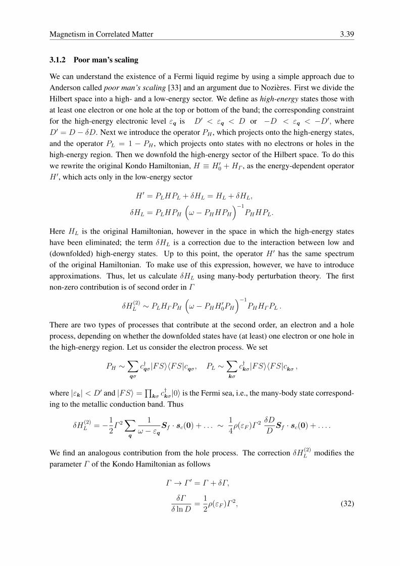
Magnetism in Correlated Matter 3.39
3.1.2 Poor man’s scaling
We can understand the existence of a Fermi liquid regime by using a simple approach due toAnderson called poor man’s scaling [33] and an argument due to Nozieres. First we divide theHilbert space into a high- and a low-energy sector. We define as high-energy states those withat least one electron or one hole at the top or bottom of the band; the corresponding constraintfor the high-energy electronic level εq is D′ < εq < D or −D < εq < −D′, whereD′ = D − δD. Next we introduce the operator PH , which projects onto the high-energy states,and the operator PL = 1 − PH , which projects onto states with no electrons or holes in thehigh-energy region. Then we downfold the high-energy sector of the Hilbert space. To do thiswe rewrite the original Kondo Hamiltonian, H ≡ H ′0 +HΓ , as the energy-dependent operatorH ′, which acts only in the low-energy sector
H ′ = PLHPL + δHL = HL + δHL,
δHL = PLHPH
(ω − PHHPH
)−1
PHHPL.
Here HL is the original Hamiltonian, however in the space in which the high-energy stateshave been eliminated; the term δHL is a correction due to the interaction between low and(downfolded) high-energy states. Up to this point, the operator H ′ has the same spectrumof the original Hamiltonian. To make use of this expression, however, we have to introduceapproximations. Thus, let us calculate δHL using many-body perturbation theory. The firstnon-zero contribution is of second order in Γ
δH(2)L ∼ PLHΓPH
(ω − PHH ′0PH
)−1
PHHΓPL .
There are two types of processes that contribute at the second order, an electron and a holeprocess, depending on whether the downfolded states have (at least) one electron or one hole inthe high-energy region. Let us consider the electron process. We set
PH ∼∑qσ
c†qσ|FS〉〈FS|cqσ, PL ∼∑kσ
c†kσ|FS〉〈FS|ckσ ,
where |εk| < D′ and |FS〉 =∏kσ c†kσ|0〉 is the Fermi sea, i.e., the many-body state correspond-
ing to the metallic conduction band. Thus
δH(2)L = −1
2Γ 2∑q
1
ω − εqSf · sc(0) + . . . ∼ 1
4ρ(εF )Γ
2 δD
DSf · sc(0) + . . . .
We find an analogous contribution from the hole process. The correction δH(2)L modifies the
parameter Γ of the Kondo Hamiltonian as follows
Γ → Γ ′ = Γ + δΓ,
δΓ
δ lnD=
1
2ρ(εF )Γ
2, (32)
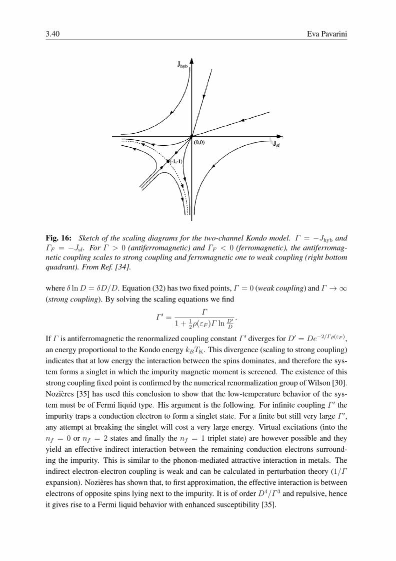
3.40 Eva Pavarini
Fig. 16: Sketch of the scaling diagrams for the two-channel Kondo model. Γ = −Jhyb andΓF = −Jsf . For Γ > 0 (antiferromagnetic) and ΓF < 0 (ferromagnetic), the antiferromag-netic coupling scales to strong coupling and ferromagnetic one to weak coupling (right bottomquadrant). From Ref. [34].
where δ lnD = δD/D. Equation (32) has two fixed points, Γ = 0 (weak coupling) and Γ →∞(strong coupling). By solving the scaling equations we find
Γ ′ =Γ
1 + 12ρ(εF )Γ ln D′
D
.
If Γ is antiferromagnetic the renormalized coupling constant Γ ′ diverges for D′ = De−2/Γρ(εF ),an energy proportional to the Kondo energy kBTK. This divergence (scaling to strong coupling)indicates that at low energy the interaction between the spins dominates, and therefore the sys-tem forms a singlet in which the impurity magnetic moment is screened. The existence of thisstrong coupling fixed point is confirmed by the numerical renormalization group of Wilson [30].Nozieres [35] has used this conclusion to show that the low-temperature behavior of the sys-tem must be of Fermi liquid type. His argument is the following. For infinite coupling Γ ′ theimpurity traps a conduction electron to form a singlet state. For a finite but still very large Γ ′,any attempt at breaking the singlet will cost a very large energy. Virtual excitations (into thenf = 0 or nf = 2 states and finally the nf = 1 triplet state) are however possible and theyyield an effective indirect interaction between the remaining conduction electrons surround-ing the impurity. This is similar to the phonon-mediated attractive interaction in metals. Theindirect electron-electron coupling is weak and can be calculated in perturbation theory (1/Γexpansion). Nozieres has shown that, to first approximation, the effective interaction is betweenelectrons of opposite spins lying next to the impurity. It is of order D4/Γ 3 and repulsive, henceit gives rise to a Fermi liquid behavior with enhanced susceptibility [35].
Magnetism in Correlated Matter 3.41
If Γ = ΓF < 0 (ferromagnetic coupling, as for example the coupling arising from directCoulomb exchange) the renormalized coupling constant Γ ′ goes to zero in the D′ → 0 limit(scaling to weak coupling). This means that the local spin becomes asymptotically free andyields a Curie-type susceptibility, which diverges for T → 0. For small but finite coupling wecan account for the ferromagnetic interaction perturbatively (expansion in orders of ΓF ). Inf -electron materials often both ferro and antiferromagnetic exchange couplings are present, thefirst, ΓF , arising from the Coulomb exchange, the second, Γ , from the hybridization. Thereare therefore two possibilities. If both exchange interactions couple the impurity with the sameconduction channel, only the total coupling ΓF + Γ matters. Thus a |ΓF | > Γ suppresses theKondo effect. If, however, ferromagnetic and antiferromagnetic exchange interaction couplethe impurity to different conduction channels, a |ΓF | > Γ does not suppress the Kondo effect(Fig. 16) but merely reduces TK. In the infinite |ΓF | limit the model describes an undercompen-sated Kondo effect [34].
3.2 The RKKY interaction
The Kondo Hamiltonian (30) describes a magnetic coupling between a local impurity and a bathof conduction electrons. Thus, in the presence of several Kondo impurities coupled to the sameconduction electron bath, an indirect magnetic coupling between the local moments arises. Letus start for simplicity from two Kondo impurities described by the Hamiltonian
H2K =∑kσ
εknkσ +∑i=1,2
ΓSif · sc(0). (33)
Let us calculate the effective magnetic coupling between the impurities by integrating out thedegrees of freedom of the conduction electrons; this can be done again via perturbation theoryor via a canonical transformation. At second order in Γ , the original Hamiltonian becomes
HRKKY = I12(R12) S1f · S2
f (34)
whereR12 = R1 −R2 and
I12(R12) ∼− Γ 2 1
Nk
∑k
1
Nk
∑q
Θ(εF − εk)Θ(εk+q − εF )cos q ·R12
εk+q − εk.
For a free-electron gas one finds
I12(R12) ∼−Γ 2q4
F
π3
[sin 2qFR12 − 2qFR12 cos 2qFR12
(2qFR12)4
],
where R12 = |R12|. The coupling I12(R12) decays as ∼ 1/R312 with the distance between
the two impurities. It oscillates with a behavior similar to Friedel oscillations; the sign ofthe interaction at a certain distance between the impurities depend on the band filling, andit is negative (ferromagnetic) for qF → 0. The exchange Hamiltonian HRKKY is known asthe Ruderman-Kittel-Kasuya-Yosida (RKKY) interaction and competes with the Kondo effect.
3.42 Eva Pavarini
We can understand this competition using the following – well known but naive – argument.For simplicity, we assume I12 > 0 (antiferromagnetic) as it is often the case. The energygain obtained forming a singlet (antiferromagnetic state) is ES ∝ −I12 ∝ −Γ 2; the Kondoenergy gain is instead EK ∝ −kBTK ∼ −De−2/ρ(εF )Γ . If the coupling constant Γ is small|ES| is larger than |EK |. In this case, the antiferromagnetic order is favored over the Kondoeffect, which would lead to the screening of local moments. In the opposite limit, i.e., whenΓ is large, the Kondo effect dominates, and the local moments are screened – thus the systemdoes not exhibit any long-range order. Although reality is more complex – the two effectsoccur together – this simple argument gives a picture of the mechanisms at play in a latticeof Kondo impurities. It is important to understand that the RKKY interaction is an indirectcoupling arising from the interaction of a correlated impurity with a conduction-electron bath;the coupling I12 is proportional to Γ 2, and the coupling Γ itself was obtained by integratingout high-energy doubly occupied states on the impurity, in a similar way as we have seen forkinetic exchange. In the U = 0 limit the coupling Γ diverges and the full construction breaksdown. Finally, in a system in which non-perturbative effects – such as the Kondo effect – play akey role, the second order Hamiltonian HRKKY is in general not even sufficient to describe theactual nature of the magnetic phenomena; to obtain HRKKY we have actually integrated out thevery interaction leading to the Kondo effect, and this is clearly incorrect in the general case.
4 Conclusion
In this lecture we introduced some of the fundamental aspects of magnetism in correlated sys-tems. We have seen two distinct regimes, the itinerant and the local-moment regime. In thefirst regime we can, in most cases, treat correlation effects in perturbation theory. In the worldof real materials this is the limit in which density-functional theory (DFT), in the local-densityapproximation or its simple extensions, works best. If the system is weakly correlated we cancalculate the linear-response function in the random-phase approximation and understand mag-netism within this approach fairly well.The opposite regime is the strong-correlation limit, in which many-body effects play a key role.In this limit perturbation theory fails and we have in principle to work with many-body meth-ods. If, however, we are interested only in magnetic phenomena, at integer filling a strongsimplification comes from mapping the original many-body Hamiltonian into an effective spinmodel. The exact solution of effective spin models requires in general numerical methods suchas the Monte Carlo or quantum Monte Carlo approach, or, when the system is small enough,exact diagonalization or Lanczos. To work with material-specific spin models we need to cal-culate the magnetic exchange parameters. Typically this is done starting from total-energy DFTcalculations for different spin configurations, e.g., in the LDA+U approximation. The LDA+Uapproach is based on the Hartree-Fock approximation, and therefore when we extract the pa-rameters from LDA+U calculations we have to keep in mind the shortcomings of the method.Furthermore if we want to extract the magnetic couplings from total energy calculations wehave to make a guess on the form of the spin model. More flexible approaches, which allow
Magnetism in Correlated Matter 3.43
us to account for actual correlation effects, are based on Green functions and the local-forcetheorem [36], or on canonical transformations [28, 37].In strongly correlated materials localized- and itinerant-moment physics can often be observedin the same system, although in different energy or temperature regimes. This is apparent in thecase of the Kondo effect. For a Kondo impurity, the susceptibility exhibits a Curie behavior athigh temperature and a Fermi liquid behavior at low temperature. In correlated transition-metaloxides Fermi liquid and local-spin magnetism can both play an important role but at differentenergy scales. Furthermore, in the absence of a large charge gap, downfolding to spin mod-els is not really justified. The modern method to bridge between the localized and itinerantregimes and deal with the actual complications of real systems is the dynamical mean-field the-ory (DMFT) [14–16]. Within this technique we directly solve generalized Hubbard-like models,albeit in the local self-energy approximation. DMFT is the first flexible approach that allows usto understand the paramagnetic Mott metal-insulator transition and thus also magnetism in cor-related materials in a realistic setting. Modern DMFT codes are slowly but steadily becomingas complex and flexible as DFT codes, allowing us to deal with the full complexity of stronglycorrelated materials. While this is a huge step forward, we have to remember that state-of-the-art many-body techniques have been developed by solving simple models within certainapproximations. We have to know these very well if we want to understand real materials andfurther advance the field. In DMFT we self-consistently solve an effective quantum impuritymodel, a generalization of the Anderson model. Thus a lot can be learnt from the solution ofthe Anderson model in the context of the Kondo problem. Much can be understood alone withsimple arguments, as Anderson or Nozieres have shown us, reaching important conclusions onthe Kondo problem with paper and pencil.
Acknowledgment
Support of the Deutsche Forschungsgemeinschaft through FOR1346 is gratefully acknowledged.
3.44 Eva Pavarini
Appendices
A Formalism
The formulas in this Appendix are in atomic units: The numerical value of e, m, and ~ is 1, thatof µB is either 1/2 (SI units) or α/2 (cgs-Gauss units), where α is the fine-structure constant;the energies are in Hartree.
A.1 Matsubara Green functionsA.1.1 Imaginary-time and frequency Green functions
The imaginary-time Matsubara Green function is defined as
Gαα′(τ ) = −〈T cα(τ1)c†α′(τ2)〉 = −
1
ZTr[e−β(H−µN)T cα(τ1)c
†α′(τ2)
],
where T is the time-ordering operator, τ = (τ1, τ2), Z = Tre−β(H−µN) is the partition function,and the imaginary-time operators o(τ) = c(τ), c†(τ) are defined as
o(τ) = eτ(H−µN)o e−τ(H−µN).
The indices α and α′ are the flavors; they can be site and spin indices in the atomic limit and kand spin indices in the non-interacting-electrons limit. Writing the action of the time-orderingoperator explicitly, we obtain
Gαα′(τ ) = −Θ(τ1 − τ2)〈cα(τ1)c†α′(τ2)〉+Θ(τ2 − τ1)〈c†α′(τ2)cα(τ1)〉.
Using the invariance of the trace of the product of operators under cyclic permutations, one canshow that the following properties hold
Gαα′(τ ) = Gαα′(τ1 − τ2),
Gαα′(τ) = −Gαα′(τ + β) for − β < τ < 0.
The Fourier transform on the Matsubara axis is
Gαα′(iνn) =1
2
∫ β
−βdτeiνnτGαα′(τ) =
∫ β
0
dτeiνnτGαα′(τ),
with νn = (2n+ 1)π/β. The inverse Fourier transform is given by
Gαα′(τ) =1
β
+∞∑n=−∞
e−iνnτGαα′(iνn).
The convergence of Gαα′(τ) is only guaranteed in the interval −β < τ < β. Finally, if nα isthe number of electrons for flavor α, one can show that
Gαα(τ → 0+) = −1 + nα, Gαα(τ → β−) = −nα. (35)
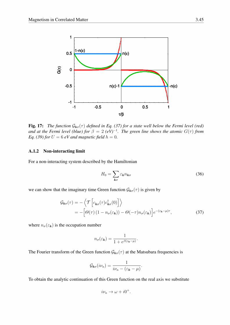
Magnetism in Correlated Matter 3.45
-1
-0.5
0
0.5
1
-1 -0.5 0 0.5 1
G( τ
)
τ/β
n(ε)
n(ε)-1 -n(ε)
1-n(ε)
-1
-0.5
0
0.5
1
-1 -0.5 0 0.5 1
G( τ
)
τ/β
n(ε)
n(ε)-1 -n(ε)
1-n(ε)
-1
-0.5
0
0.5
1
-1 -0.5 0 0.5 1
G( τ
)
τ/β
n(ε)
n(ε)-1 -n(ε)
1-n(ε)
Fig. 17: The function Gkσ(τ) defined in Eq. (37) for a state well below the Fermi level (red)and at the Fermi level (blue) for β = 2 (eV)−1. The green line shows the atomic G(τ) fromEq. (39) for U = 6 eV and magnetic field h = 0.
A.1.2 Non-interacting limit
For a non-interacting system described by the Hamiltonian
H0 =∑kσ
εknkσ (36)
we can show that the imaginary time Green function Gkσ(τ) is given by
Gkσ(τ) = −⟨T[ckσ(τ)c
†kσ(0)
]⟩= −
[Θ(τ) (1− nσ(εk))−Θ(−τ)nσ(εk)
]e−(εk−µ)τ , (37)
where nσ(εk) is the occupation number
nσ(εk) =1
1 + eβ(εk−µ).
The Fourier transform of the Green function Gkσ(τ) at the Matsubara frequencies is
Gkσ(iνn) =1
iνn − (εk − µ).
To obtain the analytic continuation of this Green function on the real axis we substitute
iνn → ω + i0+.
3.46 Eva Pavarini
A.1.3 Matsubara sums
The non-interacting Green function Gkσ(z) has a pole at zp = εk − µ; the Fermi function nσ(z)has poles for z = iνn instead. Let us consider the integral
1
2πi
∮C
Fkσ(z)nσ(z)ezτdz = 0,
where 0 < τ < β and where the function Fkσ(z) is analytic everywhere except at some poles{zp}. The contour C is a circle in the full complex plane centered at the origin and includingthe poles of the Fermi function (Matsubara frequencies) and the poles of Fkσ(z). The integralis zero because the integrand vanishes exponentially for |z| → ∞. Furthermore
Res [nσ(iνn)] = −1
β.
Using Cauchy’s integral theorem we then have
1
β
∑n
eiνnτFkσ(iνn) =∑zp
Res [Fkσ(zp)]nσ(zp)ezpτ .
We can use this expression and (35) to show that
1
β
∑n
e−iνn0−Gkσ(iνn) = Gkσ(0−) = nσ(εk),
1
β
∑n
e−iνn0+Gkσ(iνn) = Gkσ(0+) = nσ(εk)− 1.
In a similar way we can show that
1
β
∑n
eiνn0+Gkσ(iνn)Gkσ(iνn) =dnσ(εk)
dεk= βnσ(εk)[−1 + nσ(εk)],
1
β
∑n
eiνn0+Gkσ(iνn)Gk+qσ(iνn + iωm) =nk+q − nk
−iωm + εk+q − εk,
where in the last relation ωm = 2mπ/β is a bosonic Matsubara frequency.
A.1.4 Atomic limit
It is interesting to consider a half-filled idealized atom described by the Hamiltonian
H = εd∑σ
nσ + U
(N2
4− S2
z
)+ gµBhSz. (38)
For τ > 0 we can calculate explicitly the Green function, obtaining
Gσ(τ) = −1
2
1
1 + eβU/2 cosh (βgµBh/2)
[eτ(U−gµBhσ)/2 + e(β−τ)(U+gµBhσ)/2
]. (39)
Magnetism in Correlated Matter 3.47
The Fourier transform of Gσ(τ) is
Gσ(iνn) =
[w−
iνn + (U − gµBhσ)/2+
w+
iνn − (U + gµBhσ)/2
],
where
w± =1
2
1 + eβU/2e±βgµBhσ/2
1 + eβU/2 cosh (βgµBh/2).
Since the Green function is written as the sum of functions with one pole, the analytic continu-ation is simple, as in the non-interacting case. We replace iνn with ω + i0+.
A.2 Linear-response theoryA.2.1 Theory
The response of a system described by the Hamiltonian H to a small magnetic field h(r, t) isgiven by the linear correction to the Hamiltonian, i.e.,∑
ν
δHν(r; t) = −∑ν
Mν(r; t)hν(r; t), (40)
whereM (r; t) is the magnetization operator in the Heisenberg representation
Mν(r; t) = eiHtMν(r)e−iHt
and ν = x, y, z. To linear order in the perturbation and assuming that the perturbation is turnedon adiabatically at t0 = −∞
〈Mν(r; t)〉 − 〈Mν(r)〉0︸ ︷︷ ︸δ〈Mν(r; t)〉
= −i∑ν′
∫dr′∫ t
−∞dt′〈[∆Mν(r; t), δHν′(r
′; t′)]〉0.
Here 〈Mν(r)〉0 is the (equilibrium) thermal average in the absence of the perturbation and∆Mν(r; t) =Mν(r; t)− 〈Mν(r)〉0. By replacing
∑ν′ δHν′(r
′; t′) with (40) we obtain
δ〈Mν(r; t)〉 = i∑ν′
∫dr′∫ t
−∞dt′ 〈[∆Mν(r; t), ∆Mν′(r
′; t′)]〉0 hν′(r′; t′).
The function
χνν′(r, r′; t, t′) = i 〈[∆Mν(r; t), ∆Mν′(r
′; t′)]〉0Θ(t− t′) (41)
is the so-called retarded response function. If the Hamiltonian H has time translational invari-ance symmetry the retarded response function depends only on time differences t− t′. For theFourier transform, we have
δ〈Mν(r;ω)〉 =∑ν′
∫dr′χνν′(r, r
′;ω)hν′(r′;ω).
3.48 Eva Pavarini
For a system with translational invariance, we additionally have
δ〈Mν(q;ω)〉 =∑ν′
χνν′(q;ω)hν′(q;ω).
In the ω = 0 and q → 0 limit we have
χνν′(0; 0) = limhν′→0
∂Mν
∂hν′,
where hν′ = hν′(0; 0). More details can be found in Ref. [27]. In the rest of the Appendix wereplace for simplicity the notation 〈· · · 〉0 with 〈· · · 〉.
A.2.2 Kramers-Kronig relations and thermodynamic sum rule
Important properties of the spin susceptibility are the Kramers-Kronig relations
Re[χ(q;ω)]− Re[χ(q;∞)] =1
πP∫ +∞
−∞
Im[χ(q;ω′)]
ω′ − ω dω′,
Im[χ(q;ω)] = − 1
πP∫ +∞
−∞
Re[χ(q;ω′)]− Re[χ(q;∞)]
ω′ − ω dω′,
where P is the Cauchy principal value, and Re and Im indicate the real and imaginary part.The first Kramers-Kronig relation yields the sum rule
Re[χ(q;ω = 0)]− Re[χ(q;∞)] =1
πP∫ +∞
−∞
Im[χ(q;ω′)]
ω′dω′. (42)
In the q = 0 limit, Eq. (42) is known as thermodynamic sum rule.
A.2.3 Fluctuation-dissipation theorem and static susceptibility
We define the spin-spin correlation function
Sνν′(q; t) = 〈∆Sν(q; t)∆Sν′(−q)〉
where ∆Sν(q; t) = Sν(q; t) − 〈Sν(q; 0)〉 and where the Sν are spin operators. The Fouriertransform of the correlation function in frequency space is Sνν′(q;ω). One can show that
Sνν′(q;ω) = eβωSν′ν(q;−ω).
The following formula, known as fluctuation-dissipation theorem, relates the spin-spin correla-tion function with the magnetic susceptibility
Im[χνν′(q;ω)] =1
2(1 + nB)(gµB)
2Sνν′(q;ω), nB(ω) =1
eβω − 1.
Assuming kBT large and using Eq. (42) we find
Re[χνν′(q;ω = 0)]− Re[χνν′(q;∞)] ∼ (gµB)2
kBTSνν′(q; t = 0).
Magnetism in Correlated Matter 3.49
A.2.4 Imaginary-time and frequency response function
We define the susceptibility in imaginary time as
χνν′(q; τ, τ′) = 〈T ∆Mν(q; τ)∆Mν′(−q; τ ′)〉
where ∆Mν(q; τ) =Mν(q; τ)−〈Mν(q; 0)〉. As in the case of the Green function, by using theinvariance properties of the trace one can show that
χνν′(q; τ, τ′) = χνν′(q; τ − τ ′).
The response function in imaginary time is related to the response function at the bosonic Mat-subara frequency iωm through the Fourier transforms
χνν′(q; τ) =1
β
∑n
e−iωmτχνν′(q; iωm),
χνν′(q; iωm) =
∫dτeiωmτχνν′(q; τ).
A.3 Magnetic susceptibilityA.3.1 Spin and magnetization operators
The spin operators Sν are defined as
Sν =1
2
∑σσ′
c†σσνcσ′ ,
where ν = x, y, z and σν are the Pauli matrices
σx =
(0 1
1 0
)σy =
(0 −ii 0
)σz =
(1 0
0 −1
).
The magnetization operators Mν are defined as Mν = −gµBSν .
A.3.2 Matsubara magnetic susceptibility
The magnetic susceptibility for a single-band system can be expressed as
χzz(q; τ ) =(gµB)
2
4
∑σσ′
σσ′ χqσσ′(τ ) =
(gµB)2
4
∑σσ′
σσ′1
β
1
N2k
∑kk′
[χ(q; τ )]σk,σ′k′︸ ︷︷ ︸χqσσ′
(τ )
(43)
where σ = 1 or −1 depending on whether the spin is up or down, τ = (τ1, τ2 τ3, τ4) and
[χ(q; τ )]σk,σ′k′ =〈T ckσ(τ1)c†k+qσ(τ2)ck′+qσ′(τ3)c
†k′σ′(τ4)〉
−〈T ckσ(τ1)c†k+qσ(τ2)〉〈T ck′+qσ′(τ3)c
†k′σ′(τ4)〉.
3.50 Eva Pavarini
In Fourier space
χzz(q; iωm) =(gµB)
2
4
∑σσ′
σσ′1
β2
∑nn′
χqσσ′
n,n′ (iωm)
=(gµB)
2
4
∑σσ′
σσ′1
β2
∑nn′
1
β
1
N2k
∑kk′
[χ(q; iωm)]σkn,σ′k′n′︸ ︷︷ ︸χqσσ′
n,n′ (iωm)
,
where ωm = 2mπ/β is a bosonic Matsubara frequency and
χqσσ′
n,n′ (iωm) = χqσσ′(ν) =
β
8
∫∫∫dτ eiν·τχqσσ
′(τ ). (44)
The integral for each τ component is from −β to β and ν = (νn,−νn − ωm, νn′ + ωm,−νn′).
A.3.3 Symmetry properties
Let us now analyze the symmetry properties of (44). The complex conjugate is given by[χqσσ
′
n,n′ (iωm)]∗
= χqσσ′
−n−1,−n′−1(−iωm),
with
χqσσ′
n,n′ (iωm) =β
8
∫∫∫dτ ei(−ωmτ23+νnτ12+νn′τ34)χqσσ
′(τ ).
By using the fact that, for the cases considered here, the response function is real in τ space andby exchanging the indices 1 and 4, 2 and 3 in the integrand, we find
χqσσ′
n,n′ (iωm) = χqσ′σ
n′,n (iωm),
and hence if σ = σ′, νn = ν ′n is a reflection axis. An additional reflection axis can be found byfirst shifting the frequency νn = νl − ωm
χqσσ′
l,n′ (iωm) =β
8
∫∫∫dτ ei(−ωmτ13+νlτ12+νn′τ34)χqσσ
′(τ )
and then exchanging in the integrand the indices 12 with 34 and vice versa. Hence
χqσσ′
l,n′ (iωm) = χqσ′σ
n′,l (−iωm)
so that, if σ = σ′, νn+m = −νn′ is a mirror line∣∣∣χqσσ′n+m,n′(iωm)∣∣∣ = ∣∣∣χqσ′σ−n′−1,−n−m−1(iωm)
∣∣∣ .
Magnetism in Correlated Matter 3.51
A.3.4 Non-interacting limit
For a non-interacting system described by Hamiltonian (36) Wick’s theorem yields
χqσσ′(τ ) = − 1
β
1
Nk
∑k
〈T ckσ(τ1)c†k+qσ′(τ4)〉〈T ck+qσ′(τ3)c
†kσ(τ2)〉
= − 1
β
1
Nk
∑k
Gkσ(τ14)Gk+qσ′(−τ23)δσ,σ′ .
Then, in the paramagnetic case, the magnetic susceptibility is given by
χzz(q; τ ) = −(gµB)21
4
1
β
1
Nk
∑kσ
Gkσ(τ14)Gk+qσ(−τ23).
Its Fourier transform is
χzz(q; iωm) = (gµB)21
4
1
β2
∑nn′
∑σ
χqσσn,n′(iωm),
where ∑σ
χqσσn,n′(iωm) = −β1
Nk
∑kσ
Gkσ(iνn)Gk+qσ(iνn + iωm)δn,n′ .
Thus, the static susceptibility is
χzz(q; 0) = − (gµB)2 1
4
1
Nk
∑kσ
nσ(εk+q)− nσ(εk)εk+q − εk
.
Finally, in the q → 0 and T → 0 limit we find
χzz(0; 0) =1
4(gµB)
2 1
Nk
∑kσ
[−dnσ(εk)
dεk
]T=0︸ ︷︷ ︸
ρ(εF )
=1
4(gµB)
2 ρ(εF ).
A.3.5 Atomic limit
In the atomic limit, we sum over q to obtain the local susceptibility tensor
χσσ′(τ ) =
1
Nk
∑q
χqσσ′(τ ).
For Hamiltonian (38), in the sector τ+ such that τi > τi+1, the latter has the form
χσσ′(τ+) =
1
β
1
2(1 + eβU/2)
(eτ12U/2+τ34U/2 + δσσ′e
(β−τ12)U/2−τ34U/2).
The magnetic susceptibility for τi > τi+1 is then given by
χzz(τ+) = (gµB)
2 1
4
∑σσ′
σσ′χσσ′(τ+) =
(gµB)2
4β
1
(1 + eβU/2)e(β−τ12−τ34)U/2,
3.52 Eva Pavarini
which depends only on τ = τ12+τ34. In the remaining sectors (labeled with P ) the susceptibilityhas a similar form after appropriate permutation of the imaginary times
χzz(τP ) = (gµB)
2 1
4
∑σσ′
σσ′χσσ′(τ P ) = sP
(gµB)2
4βn(−sP y)e−sP (τ12+τ34)y,
where y = U/2 and sP = ±1; the derivation can be found in [27]. If we perform the Fouriertransform of χzz(τ ) we find χzz(iωn) = χzz(0)δωn,0. The static susceptibility is
χzz(0) = (gµB)2 1
4kBT
eβU/2
1 + eβU/2= (gµB)
2 1
4
1
β2
∑nn′
∑σσ′
σσ′ χσσ′
n,n′(0).
Here, after setting
Mn =
[1
iνn − y− 1
iνn + y
]we have∑
σσ′
σσ′ χσσ′
n,n′(0) =dMn′Mn
dy− βn(y)
[δn,n′
dMn
dy+ δn,−n′−1
dMn′
dy
]+ βn(−y)MnMn′
−1
y
[Mn′−βn(y)δn,−n′−1 + βn(−y)δn,n′
]Mn.
Most contributions cancel each other when the sums over the Matsubara frequencies are per-formed. A detailed derivation can be found in Ref. [27]. For y = 0 only the terms proportionalto δn,n′ survive, as expected from the Wick theorem.
Magnetism in Correlated Matter 3.53
References
[1] P. Weiss, J. Phys. Theor. Appl. 6, 661 (1907)
[2] F. Hund, Z. Phys. 33, 855 (1925)
[3] W. Heisenberg, Z. Phys. 49, 619 (1928)
[4] C.G. Shull and J.S. Smart, Phys. Rev. 76, 1256 (1949)
[5] L. Neel, Ann. de Phys. 17, 5 (1932); ibid. 5, 232 (1936); C. R. Acad. Sc. 203, 304 (1936)
[6] H. Bethe, Z. Phys. 71, 205 (1931)
[7] P.W. Anderson, Phys. Rev. 86, 694 (1952)
[8] P.W. Anderson, Phys. Rev. 130, 439 (1963)
[9] P.W. Higgs, Phys. Rev. Lett. 13, 508 (1964)
[10] J. Kondo, Prog. Theor. Phys. 32, 37 (1964)
[11] K. Andres, J.E. Graebner and H.R. Ott, Phys. Rev. Lett. 35, 1779 (1975)
[12] A.C. Hewson: The Kondo Problem to Heavy Fermions(Cambridge University Press, 1993)
[13] J.G. Bednorz, K.A. Muller, Z. Phys. B 64, 189 (1986)
[14] W. Metzner and D. Vollhardt, Phys. Rev. Lett. 62, 324 (1989);A. Georges and G. Kotliar, Phys. Rev. B 45, 6479 (1992)
[15] E. Pavarini, E. Koch, A. Lichtenstein, D. Vollhardt:The LDA+DMFT approach to strongly correlated materials,Reihe Modeling and Simulation, Vol. 1 (Forschungszentrum Julich, 2011)http://www.cond-mat.de/events/correl11
[16] E. Pavarini, E. Koch, A. Lichtenstein, D. Vollhardt: DMFT at 25: Infinite Dimensions,Reihe Modeling and Simulation, Vol. 4 (Forschungszentrum Julich, 2014)http://www.cond-mat.de/events/correl14
[17] H. Bruus and K. Flensberg: Many-Body Quantum Theory in Condensed Matter Physics(Oxford University Press, 2004)
[18] P. Fazekas: Lecture Notes on Electron Correlation and Magnetism(World Scientific, Singapore, 1999)
[19] D.C. Matthis: The Theory of Magnetism Made Simple (World Scientific, Singapore, 2006)
3.54 Eva Pavarini
[20] K. Yosida: Theory of Magnetism (Springer, Heidelberg, 1998)
[21] E. Pavarini, E. Koch, F. Anders, M. Jarrell:Correlated electrons: from models to materials,Reihe Modeling and Simulation, Vol. 2 (Forschungszentrum Julich, 2012)http://www.cond-mat.de/events/correl12
[22] E. Pavarini, E. Koch, U. Schollwock:Emergent Phenomena in Correlated Matter,Reihe Modeling and Simulation, Vol. 3 (Forschungszentrum Julich, 2013)http://www.cond-mat.de/events/correl13
[23] See R. Eder, Multiplets in Transition Metal Ions in Ref. [21]
[24] See E. Pavarini, Crystal-field Theory, Tight-binding Method and Jahn-Teller Effect,in Ref. [21]
[25] See E. Pavarini, The LDA+DMFT Approach, in Ref. [15]
[26] See E. Koch, Exchange Mechanisms, in Ref. [21]
[27] See E. Pavarini, Linear-response Theory, in Ref. [16]
[28] J.R. Schrieffer and P.A. Wolff, Phys. Rev. 149, 491 (1966);A.H. MacDonald, S.M. Girvin and D. Yoshioka, Phys. Rev. B 37, 9753 (1988)
[29] E. Pavarini, I. Dasgupta, T.Saha-Dasgupta, O. Jepsen and O.K. Andersen,Phys. Rev. Lett. 87, 047003 (2001)
[30] K. Wilson, Rev. Mod. Phys. 47, 773 (1975)
[31] N. Andrei, K. Furuya, and J.H. Lowenstein, Rev. Mod. Phys. 55, 331 (1983);A.M. Tsvelik and P.B. Wiegmann, Adv. Phys. 32, 453 (1983)
[32] J.E. Gubernatis, J.E. Hirsch, and D.J. Scalapino, Phys. Rev. B 16, 8478 (1987)
[33] P.W. Anderson, J. Phys. C: Solid State Phys. 3, 2436 (1970)
[34] E. Pavarini and L.C. Andreani, Phys. Rev. Lett. 77, 2762 (1996)
[35] P. Nozieres, J. Low. Temp. Phys. 17, 31 (1974)
[36] A.I. Lichtenstein, M.I. Katsnelson, and V.A. Gubanov, J. Phys. F 14, L125;Solid State Commun. 54, 327 (1985);A.I. Lichtenstein, M.I. Katsnelson, V.P. Antropov, and V.A. Gubanov,J. Magn. Magn. Mater. 67, 65 (1987);M.I. Katsnelson and A.I. Lichtenstein, Phys. Rev. B 61, 8906 (2000)
Magnetism in Correlated Matter 3.55
[37] E. Pavarini, E. Koch, and A.I. Lichtenstein,Phys. Rev. Lett. 101, 266405 (2008);A. Chiesa, S. Carretta, P. Santini, G. Amoretti and E. Pavarini,Phys. Rev. Lett. 110, 157204 (2013)


![Journal of Magnetism and Magnetic Materialsof high temperature superconductivity [11–17] and more generally correlated physics in complex oxides materials [6,18,19]. Towards this](https://img.dokumen.tips/doc/110x75/5f268f96f8de0d2e6d643af2/journal-of-magnetism-and-magnetic-materials-of-high-temperature-superconductivity.jpg)