PHYSICAL REVIEW E 90, 043010 (2014)

Magnetic field reversals and long-time memory in conducting flows

P. Dmitruk,1 P. D. Mininni,1 A. Pouquet,2 S. Servidio,3 and W. H. Matthaeus4

1Departamento de Fısica, Facultad de Ciencias Exactas y Naturales, Universidad de Buenos Aires and IFIBA,CONICET, Buenos Aires, Argentina

2Department of Atmospheric and Space Physics, University of Colorado and National Center for Atmospheric Research,Boulder, Colorado, USA

3Dipartimento di Fisica, Universita della Calabria, Cosenza, Italy4Bartol Research Institute and Department of Physics and Astronomy, University of Delaware, Newark, Delaware, USA

(Received 10 December 2013; revised manuscript received 17 July 2014; published 16 October 2014)

Employing a simple ideal magnetohydrodynamic model in spherical geometry, we show that the presenceof either rotation or finite magnetic helicity is sufficient to induce dynamical reversals of the magnetic dipolemoment. The statistical character of the model is similar to that of terrestrial magnetic field reversals, with thesimilarity being stronger when rotation is present. The connection between long-time correlations, 1/f noise,and statistics of reversals is supported, consistent with earlier suggestions.

DOI: 10.1103/PhysRevE.90.043010 PACS number(s): 47.65.−d, 47.27.E−, 47.35.Tv, 91.25.Mf

I. INTRODUCTION

The origin of magnetic field reversals in Earth’s magneticfield is a matter of debate. Reversals take place rapidly, withina scale of ∼1000 years, but infrequently, distanced apart byperiods of 104–107 years [1,2].

Reversals, first thought to be a purely random process, arenow known to display long-term memory with deviations froma purely Poisson process [3]. In many systems, such a highdegree of variability may be associated with features of thepower spectrum of the time series known as “1/f ” noise, anindication of the presence of correlations over a wide range oftime scales [4–7]. 1/f signals are found in many physicalsystems [8,9], including the intensity of the geomagneticfield [10,11]. We examine this phenomenon by employinga simple model consisting of incompressible nondissipativemagnetohydrodynamics (MHD) in spherical geometry. Theresults demonstrate the presence of reversals possessing 1/f

noise where rotation and/or magnetic helicity play importantroles. Remarkably, the distribution of waiting times betweenreversals follows a power law that is comparable to the recordof terrestrial magnetic reversals.

Earth’s magnetic field is sustained by a dynamo process:Motions of the conducting fluid core generate and sustainmagnetic fields against Ohmic dissipation. Although MHDcontains the basic physics of the dynamo, the completeterrestrial problem requires solving either compressible,Boussinesq, or anelastic MHD equations for the velocity, themagnetic field, and the temperature, in a spherical shell witha possible inner solid conducting core, and surrounded by amantle [12,13]. Additional realism requires more complexityin chemistry, equations of state, and boundary conditions.Even with advanced supercomputers, only few reversals canbe simulated [12–14], and studies of the long-time statistics ofreversals are therefore out of reach.

Experiments reproducing dynamos in laboratory turbulentflows display magnetic field reversals [15,16], 1/f noise, andlong-term memory. Still, a theoretical understanding of thesefeatures remains incomplete since the origin of correlationswith time scales much greater than the characteristic nonlineartime associated with the largest eddies in the system isunknown.

Many physical causes have been considered to explain theorigin and statistics of the reversals, including the effect oftides, departures of the mantle from spherical geometry, or lowmagnetic Reynolds number effects. We show that the MHDequations in their simplest nonlinear form (incompressibleand ideal) in a simple geometry (spherical surrounded by aperfect conductor) already include the ingredients required formagnetic field reversals, long-time correlations, 1/f noise,and non-Poisson statistics compatible with that observed inthe geodynamo.

II. MODEL

The ideal MHD equations are solved using a spectralmethod that preserves to numerical accuracy all ideal quadraticinvariants with no numerical dissipation or dispersion. For verylong-time integrations, this is the only method that ensuresadequate conservation. Since the initial energy introduced inthe system is conserved, no external forces are needed tosustain the velocity and magnetic fields. For a purely spectralGalerkin method, we use spherical Chandrasekhar-Kendallfunctions as a basis, expanding the fields in spectral space[17,18]. A fourth-order Runge-Kutta method is used to evolvethe system in time.

With the magnetic field confined in the interior of thesphere, the system has two quadratic conserved quantities: thetotal energy (kinetic plus magnetic, E = 1

2

∫ |v|2 + |b|2 dV ,with v, b the velocity and magnetic fields) and the magnetichelicity (Hm = ∫

a · b dV , a measure of linkage or handednessof the magnetic field, with a the vector potential, ∇×a = b).E is transferred towards small scales (“direct cascade”), whileHm is transferred towards large scales (“inverse cascade”).In the ideal system, Hm condenses at the largest availablescales [19]. In our simulations, long-time-scale correlationsarise when Hm is nonzero. Long-time correlations also arisedue to symmetry breaking by rotation [20]. Here we show forthe rotating sphere that the magnetic dipole moment reverseswith respect to the rotation direction, displaying 1/f noiseand long-term memory even when the magnetic helicity iszero. A recent related study [21] reported persistence of themagnetic dipole associated with broken ergodicity effects [22].Broken ergodicity of fluid systems may also be viewed as

1539-3755/2014/90(4)/043010(7) 043010-1 ©2014 American Physical Society

DMITRUK, MININNI, POUQUET, SERVIDIO, AND MATTHAEUS PHYSICAL REVIEW E 90, 043010 (2014)

“delayed ergodicity” in which very long-time correlationsdelay ergodically covering the phase space [23].

The incompressible ideal MHD equations solved for theevolution of the velocity field v and magnetic field b (inAlfvenic units) are

∂v∂t

= v×ω + j×b − ∇(P + v2

2

)− 2�×v, (1)

∂b∂t

= ∇×(v×b), (2)

for vorticity ω = ∇×v; electric current density j = ∇×b;normalized pressure P; and rotation rate �. The units arenormalized to the spherical radius R and initial root meansquare velocity v0 = 〈v2〉1/2, so R = 1 and v0 = 1, and thetime unit is t0 = R/v0 = 1 (later time scales are rescaled toMa = 106 years, based on the longest observed waiting timebetween reversals). We consider vanishing normal velocityand magnetic field components at the sphere boundary. Forthe simulations, 980 coupled Chandrasekhar-Kendall (C-K)modes are followed in time. The C-K functions are

Ji = λ∇×rψi + ∇×(∇×rψi), (3)

where we work with a set of spherical orthonormal unitvectors (r ,θ ,φ), and the scalar function ψi is a solution ofthe Helmholtz equation, (∇2 + λ2)ψi = 0. The explicit formof ψi is

ψi(r,θ,φ) = Cql jl(|λql|r)Ylm(θ,φ), (4)

where jl(|λql|r) is the order-l spherical Bessel function ofthe first kind, {λql} are the roots of jl indexed by q (so thatthe function vanishes at r = 1), and Ylm(θ,φ) is a sphericalharmonic in the polar angle θ and the azimuthal angle φ.The subindex i is a shorthand notation for the three indices(q,l,m); q = 1,2,3, . . . corresponds to the positive values of λ,and q = −1,−2,−3, . . . indexes the negative values; finallyl = 1,2,3, . . . , and −l � m � l. The C-K functions satisfy

∇×Ji = λiJi . (5)

With the proper normalization constants, they are a completeorthonormal set. The values of |λi | play a role similar tothe wave number k in a Fourier expansion. Note that theboundary conditions, as well as the Galerkin method to solvethe equations inside the sphere using this base, were chosen toensure conservation of all quadratic invariants of the system(total energy and magnetic helicity).

The initially excited modes for the runs are those forq = ±3, l = 3 and all possible values of m. With proper initialvalues for the expansion coefficients of the C-K functions, theinitial values of the quadratic quantities can be chosen. In allthe runs, the initial total energy is set to E = 1 (dimensionlessunits). We set the initial magnetic and kinetic energies toEm = Ek ≈ 0.5. The runs with nonzero magnetic helicity haveHm ≈ 0.03. As a comparison, note that for the q = 3, l = 3mode alone, Hm/Em is no more than about 0.072 (this isthe maximum value of |Hm/Em| if only modes with |q| = 3,l = 3, and one sign of λ are excited). So, the chosen valueof Hm (when is nonzero) corresponds to about 85% of themaximum helicity in the system.

FIG. 1. (Color online) The ratio of kinetic energy vs magneticenergy Ek/Em as a function of time, for three runs with different initialconditions and same Hm = 0.03, � = 16. Thicker line (black online)Ek/Em(t = 0) = 1, intermediate thick line (red online) Ek/Em(t =0) = 0.5, and thin line (blue online) Ek/Em(t = 0) = 2.

III. RESULTS

A. Kinetic and magnetic energy, field structure

The values of the total energy E and magnetic helicityremain constant in time (as ideal invariants). The values of themagnetic and kinetic energies Em and Ek fluctuate, reachinga statistical steady state after about 20 unit times. The initialratio of kinetic over magnetic energy is Ek/Em(t = 0) = 1and approaches and fluctuates around Ek/Em ≈ 0.9. We per-formed two additional runs starting from different initial ratiosEk/Em(0) ≈ 2 and Ek/Em(0) ≈ 0.5, with the same value ofmagnetic helicity Hm = 0.03. Both cases evolve initially andafter about 20 unit times reach the same asymptotical statisticalstate, with a value of Ek/Em ≈ 0.9. This is shown in Fig. 1.This asymptotic value corresponds to a steady state withsome excess of magnetic energy over kinetic energy which isconsistent with the nonzero value of magnetic helicity (whichallows condensation at the large scales).

The results about the statistics of the magnetic dipole thatfollows (next subsection) are not sensitive to the differentinitial values of the ratio Ek/Em.

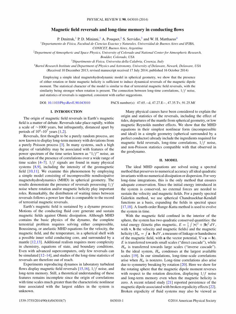
The fields evolve to a highly disordered state, with a widerange of scales present. Figure 2 shows velocity and magneticfield lines for one particular run.

B. Magnetic dipole and statistics of reversals

We focus on the dynamics of the magnetic dipole moment,

μ = 1

2

∫r×j dV, (6)

and, in particular, on its z component μz, which is ofimportance with rotation � = �z. We report first results ofa run with both nonzero magnetic helicity (Hm = 0.03) andnonzero rotation (� = 16 in units of t−1

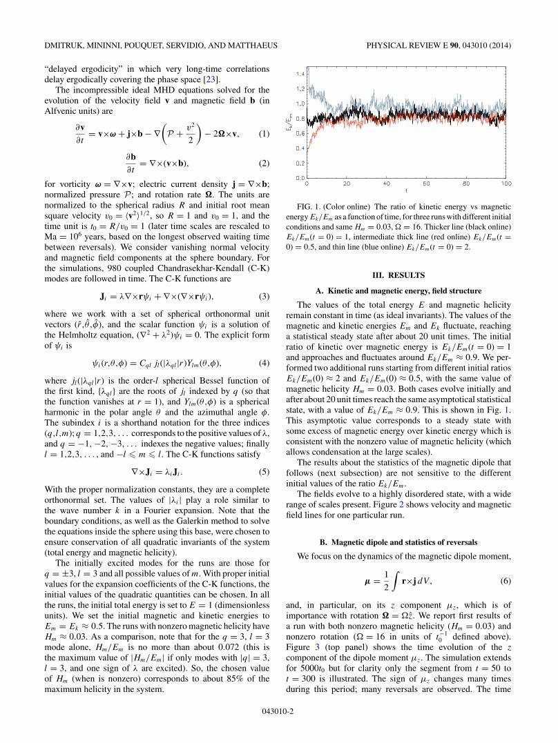
0 defined above).Figure 3 (top panel) shows the time evolution of the zcomponent of the dipole moment μz. The simulation extendsfor 5000t0 but for clarity only the segment from t = 50 tot = 300 is illustrated. The sign of μz changes many timesduring this period; many reversals are observed. The time

043010-2

MAGNETIC FIELD REVERSALS AND LONG-TIME MEMORY . . . PHYSICAL REVIEW E 90, 043010 (2014)

FIG. 2. (Color online) Velocity (top) and magnetic (bottom) fieldlines in the run with � = 16, Hm = 0.03. The field lines change coloraccording to the intensity of the field, from red to yellow, blue, andmagenta. The red, green, and blue arrows indicate, respectively, thex,y,z axis, with � in the z direction.

periods between reversals range from short times (δt ∼ 1) tolong times (δt ∼ 50).

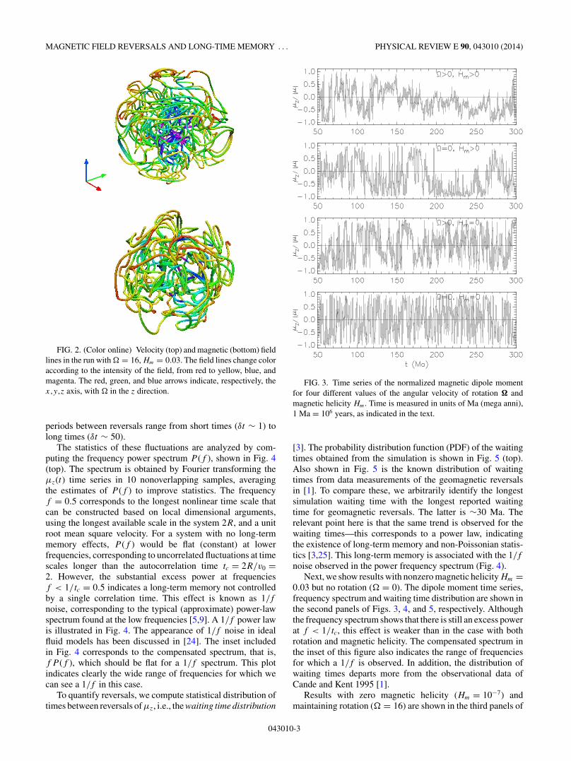
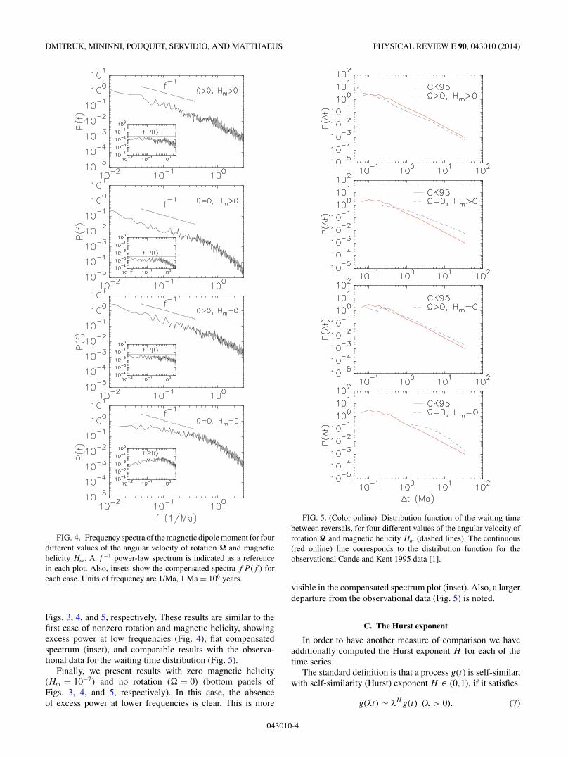
The statistics of these fluctuations are analyzed by com-puting the frequency power spectrum P (f ), shown in Fig. 4(top). The spectrum is obtained by Fourier transforming theμz(t) time series in 10 nonoverlapping samples, averagingthe estimates of P (f ) to improve statistics. The frequencyf = 0.5 corresponds to the longest nonlinear time scale thatcan be constructed based on local dimensional arguments,using the longest available scale in the system 2R, and a unitroot mean square velocity. For a system with no long-termmemory effects, P (f ) would be flat (constant) at lowerfrequencies, corresponding to uncorrelated fluctuations at timescales longer than the autocorrelation time tc = 2R/v0 =2. However, the substantial excess power at frequenciesf < 1/tc = 0.5 indicates a long-term memory not controlledby a single correlation time. This effect is known as 1/f

noise, corresponding to the typical (approximate) power-lawspectrum found at the low frequencies [5,9]. A 1/f power lawis illustrated in Fig. 4. The appearance of 1/f noise in idealfluid models has been discussed in [24]. The inset includedin Fig. 4 corresponds to the compensated spectrum, that is,f P (f ), which should be flat for a 1/f spectrum. This plotindicates clearly the wide range of frequencies for which wecan see a 1/f in this case.

To quantify reversals, we compute statistical distribution oftimes between reversals of μz, i.e., the waiting time distribution

FIG. 3. Time series of the normalized magnetic dipole momentfor four different values of the angular velocity of rotation � andmagnetic helicity Hm. Time is measured in units of Ma (mega anni),1 Ma = 106 years, as indicated in the text.

[3]. The probability distribution function (PDF) of the waitingtimes obtained from the simulation is shown in Fig. 5 (top).Also shown in Fig. 5 is the known distribution of waitingtimes from data measurements of the geomagnetic reversalsin [1]. To compare these, we arbitrarily identify the longestsimulation waiting time with the longest reported waitingtime for geomagnetic reversals. The latter is ∼30 Ma. Therelevant point here is that the same trend is observed for thewaiting times—this corresponds to a power law, indicatingthe existence of long-term memory and non-Poissonian statis-tics [3,25]. This long-term memory is associated with the 1/f

noise observed in the power frequency spectrum (Fig. 4).Next, we show results with nonzero magnetic helicity Hm =

0.03 but no rotation (� = 0). The dipole moment time series,frequency spectrum and waiting time distribution are shown inthe second panels of Figs. 3, 4, and 5, respectively. Althoughthe frequency spectrum shows that there is still an excess powerat f < 1/tc, this effect is weaker than in the case with bothrotation and magnetic helicity. The compensated spectrum inthe inset of this figure also indicates the range of frequenciesfor which a 1/f is observed. In addition, the distribution ofwaiting times departs more from the observational data ofCande and Kent 1995 [1].

Results with zero magnetic helicity (Hm = 10−7) andmaintaining rotation (� = 16) are shown in the third panels of

043010-3

DMITRUK, MININNI, POUQUET, SERVIDIO, AND MATTHAEUS PHYSICAL REVIEW E 90, 043010 (2014)

FIG. 4. Frequency spectra of the magnetic dipole moment for fourdifferent values of the angular velocity of rotation � and magnetichelicity Hm. A f −1 power-law spectrum is indicated as a referencein each plot. Also, insets show the compensated spectra f P (f ) foreach case. Units of frequency are 1/Ma, 1 Ma = 106 years.

Figs. 3, 4, and 5, respectively. These results are similar to thefirst case of nonzero rotation and magnetic helicity, showingexcess power at low frequencies (Fig. 4), flat compensatedspectrum (inset), and comparable results with the observa-tional data for the waiting time distribution (Fig. 5).

Finally, we present results with zero magnetic helicity(Hm = 10−7) and no rotation (� = 0) (bottom panels ofFigs. 3, 4, and 5, respectively). In this case, the absenceof excess power at lower frequencies is clear. This is more

FIG. 5. (Color online) Distribution function of the waiting timebetween reversals, for four different values of the angular velocity ofrotation � and magnetic helicity Hm (dashed lines). The continuous(red online) line corresponds to the distribution function for theobservational Cande and Kent 1995 data [1].

visible in the compensated spectrum plot (inset). Also, a largerdeparture from the observational data (Fig. 5) is noted.

C. The Hurst exponent

In order to have another measure of comparison we haveadditionally computed the Hurst exponent H for each of thetime series.

The standard definition is that a process g(t) is self-similar,with self-similarity (Hurst) exponent H ∈ (0,1), if it satisfies

g(λt) ∼ λHg(t) (λ > 0). (7)

043010-4

MAGNETIC FIELD REVERSALS AND LONG-TIME MEMORY . . . PHYSICAL REVIEW E 90, 043010 (2014)

-0.2

0

0.2

0.4

0.6

0.8

1

10-2 10-1 100 101 102 103 104

C(δ

)

δ

(I)

(II)

(III)

(IV)

(I) Hm=0, Ω=0(II) Hm=0, Ω>0(III) Hm>0, Ω=0(IV) Hm>0, Ω>0

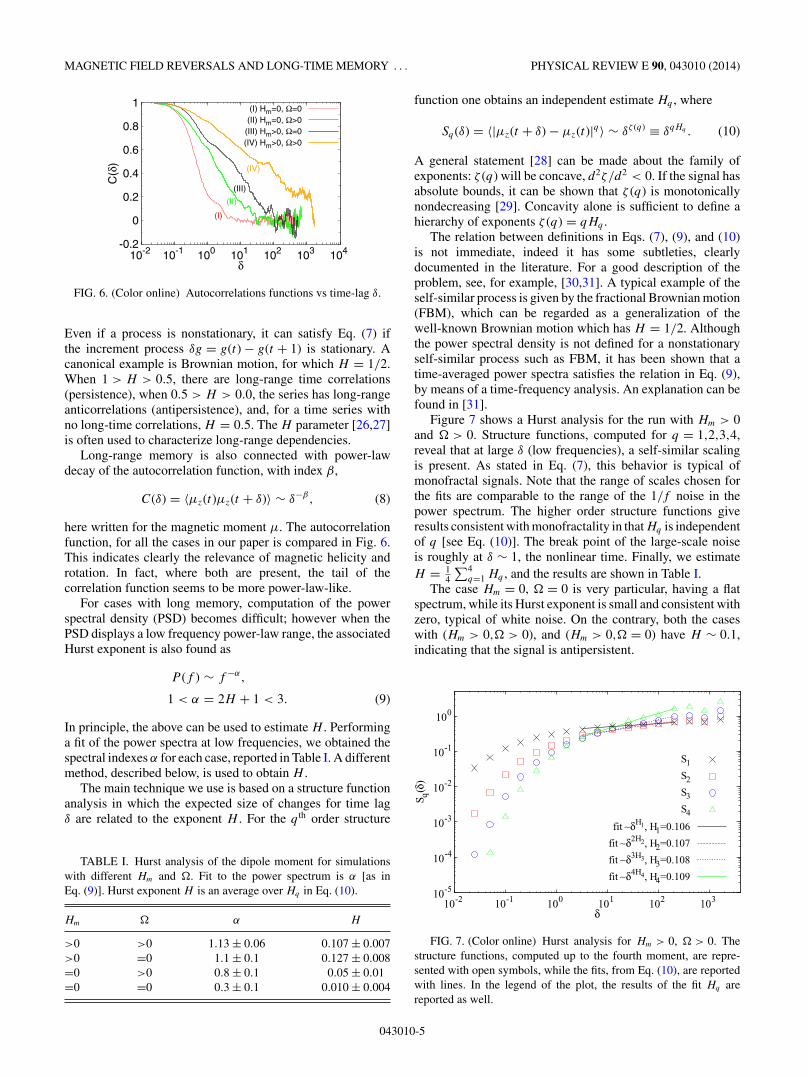
FIG. 6. (Color online) Autocorrelations functions vs time-lag δ.

Even if a process is nonstationary, it can satisfy Eq. (7) ifthe increment process δg = g(t) − g(t + 1) is stationary. Acanonical example is Brownian motion, for which H = 1/2.When 1 > H > 0.5, there are long-range time correlations(persistence), when 0.5 > H > 0.0, the series has long-rangeanticorrelations (antipersistence), and, for a time series withno long-time correlations, H = 0.5. The H parameter [26,27]is often used to characterize long-range dependencies.

Long-range memory is also connected with power-lawdecay of the autocorrelation function, with index β,

C(δ) = 〈μz(t)μz(t + δ)〉 ∼ δ−β, (8)

here written for the magnetic moment μ. The autocorrelationfunction, for all the cases in our paper is compared in Fig. 6.This indicates clearly the relevance of magnetic helicity androtation. In fact, where both are present, the tail of thecorrelation function seems to be more power-law-like.

For cases with long memory, computation of the powerspectral density (PSD) becomes difficult; however when thePSD displays a low frequency power-law range, the associatedHurst exponent is also found as

P (f ) ∼ f −α,

1 < α = 2H + 1 < 3. (9)

In principle, the above can be used to estimate H . Performinga fit of the power spectra at low frequencies, we obtained thespectral indexes α for each case, reported in Table I. A differentmethod, described below, is used to obtain H .

The main technique we use is based on a structure functionanalysis in which the expected size of changes for time lagδ are related to the exponent H . For the q th order structure

TABLE I. Hurst analysis of the dipole moment for simulationswith different Hm and �. Fit to the power spectrum is α [as inEq. (9)]. Hurst exponent H is an average over Hq in Eq. (10).

Hm � α H

>0 >0 1.13 ± 0.06 0.107 ± 0.007>0 =0 1.1 ± 0.1 0.127 ± 0.008=0 >0 0.8 ± 0.1 0.05 ± 0.01=0 =0 0.3 ± 0.1 0.010 ± 0.004

function one obtains an independent estimate Hq , where

Sq(δ) = 〈|μz(t + δ) − μz(t)|q〉 ∼ δζ (q) ≡ δqHq . (10)

A general statement [28] can be made about the family ofexponents: ζ (q) will be concave, d2ζ/d2 < 0. If the signal hasabsolute bounds, it can be shown that ζ (q) is monotonicallynondecreasing [29]. Concavity alone is sufficient to define ahierarchy of exponents ζ (q) = qHq .

The relation between definitions in Eqs. (7), (9), and (10)is not immediate, indeed it has some subtleties, clearlydocumented in the literature. For a good description of theproblem, see, for example, [30,31]. A typical example of theself-similar process is given by the fractional Brownian motion(FBM), which can be regarded as a generalization of thewell-known Brownian motion which has H = 1/2. Althoughthe power spectral density is not defined for a nonstationaryself-similar process such as FBM, it has been shown that atime-averaged power spectra satisfies the relation in Eq. (9),by means of a time-frequency analysis. An explanation can befound in [31].

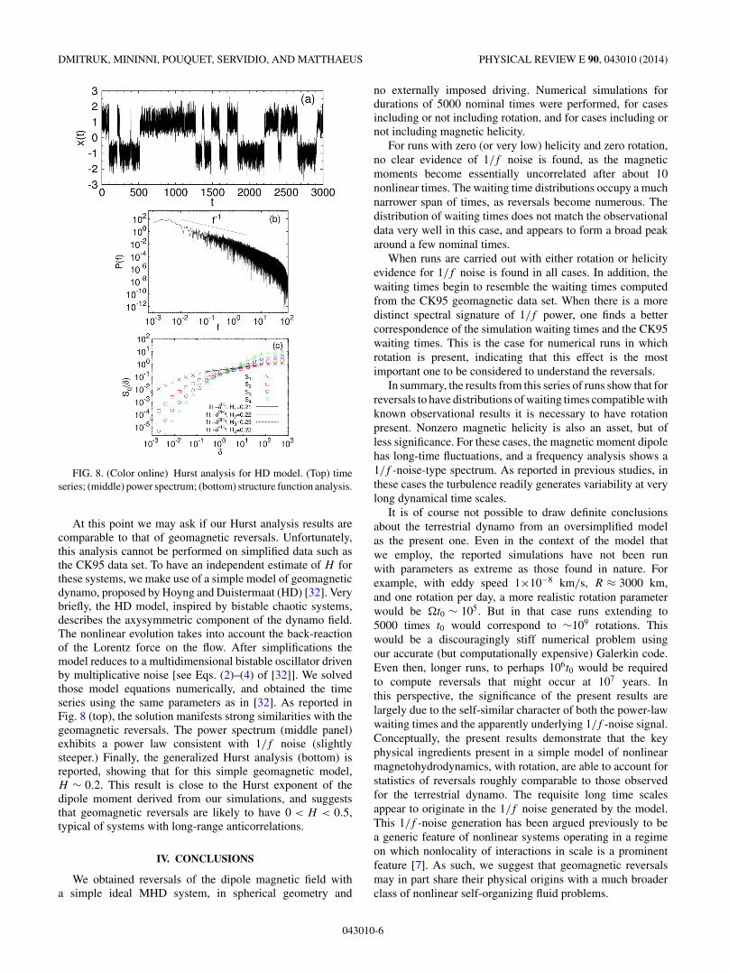
Figure 7 shows a Hurst analysis for the run with Hm > 0and � > 0. Structure functions, computed for q = 1,2,3,4,reveal that at large δ (low frequencies), a self-similar scalingis present. As stated in Eq. (7), this behavior is typical ofmonofractal signals. Note that the range of scales chosen forthe fits are comparable to the range of the 1/f noise in thepower spectrum. The higher order structure functions giveresults consistent with monofractality in that Hq is independentof q [see Eq. (10)]. The break point of the large-scale noiseis roughly at δ ∼ 1, the nonlinear time. Finally, we estimateH = 1

4

∑4q=1 Hq , and the results are shown in Table I.

The case Hm = 0, � = 0 is very particular, having a flatspectrum, while its Hurst exponent is small and consistent withzero, typical of white noise. On the contrary, both the caseswith (Hm > 0,� > 0), and (Hm > 0,� = 0) have H ∼ 0.1,indicating that the signal is antipersistent.

10-5

10-4

10-3

10-2

10-1

100

10-2 10-1 100 101 102 103

S q(δ

)

δ

S1

S2

S3

S4

fit ∼δH1, H1=0.106

fit ∼δ2H2, H2=0.107

fit ∼δ3H3, H3=0.108

fit ∼δ4H4, H4=0.109

FIG. 7. (Color online) Hurst analysis for Hm > 0, � > 0. Thestructure functions, computed up to the fourth moment, are repre-sented with open symbols, while the fits, from Eq. (10), are reportedwith lines. In the legend of the plot, the results of the fit Hq arereported as well.

043010-5

DMITRUK, MININNI, POUQUET, SERVIDIO, AND MATTHAEUS PHYSICAL REVIEW E 90, 043010 (2014)

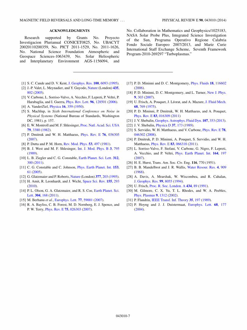
FIG. 8. (Color online) Hurst analysis for HD model. (Top) timeseries; (middle) power spectrum; (bottom) structure function analysis.

At this point we may ask if our Hurst analysis results arecomparable to that of geomagnetic reversals. Unfortunately,this analysis cannot be performed on simplified data such asthe CK95 data set. To have an independent estimate of H forthese systems, we make use of a simple model of geomagneticdynamo, proposed by Hoyng and Duistermaat (HD) [32]. Verybriefly, the HD model, inspired by bistable chaotic systems,describes the axysymmetric component of the dynamo field.The nonlinear evolution takes into account the back-reactionof the Lorentz force on the flow. After simplifications themodel reduces to a multidimensional bistable oscillator drivenby multiplicative noise [see Eqs. (2)–(4) of [32]]. We solvedthose model equations numerically, and obtained the timeseries using the same parameters as in [32]. As reported inFig. 8 (top), the solution manifests strong similarities with thegeomagnetic reversals. The power spectrum (middle panel)exhibits a power law consistent with 1/f noise (slightlysteeper.) Finally, the generalized Hurst analysis (bottom) isreported, showing that for this simple geomagnetic model,H ∼ 0.2. This result is close to the Hurst exponent of thedipole moment derived from our simulations, and suggeststhat geomagnetic reversals are likely to have 0 < H < 0.5,typical of systems with long-range anticorrelations.

IV. CONCLUSIONS

We obtained reversals of the dipole magnetic field witha simple ideal MHD system, in spherical geometry and

no externally imposed driving. Numerical simulations fordurations of 5000 nominal times were performed, for casesincluding or not including rotation, and for cases including ornot including magnetic helicity.

For runs with zero (or very low) helicity and zero rotation,no clear evidence of 1/f noise is found, as the magneticmoments become essentially uncorrelated after about 10nonlinear times. The waiting time distributions occupy a muchnarrower span of times, as reversals become numerous. Thedistribution of waiting times does not match the observationaldata very well in this case, and appears to form a broad peakaround a few nominal times.

When runs are carried out with either rotation or helicityevidence for 1/f noise is found in all cases. In addition, thewaiting times begin to resemble the waiting times computedfrom the CK95 geomagnetic data set. When there is a moredistinct spectral signature of 1/f power, one finds a bettercorrespondence of the simulation waiting times and the CK95waiting times. This is the case for numerical runs in whichrotation is present, indicating that this effect is the mostimportant one to be considered to understand the reversals.

In summary, the results from this series of runs show that forreversals to have distributions of waiting times compatible withknown observational results it is necessary to have rotationpresent. Nonzero magnetic helicity is also an asset, but ofless significance. For these cases, the magnetic moment dipolehas long-time fluctuations, and a frequency analysis shows a1/f -noise-type spectrum. As reported in previous studies, inthese cases the turbulence readily generates variability at verylong dynamical time scales.

It is of course not possible to draw definite conclusionsabout the terrestrial dynamo from an oversimplified modelas the present one. Even in the context of the model thatwe employ, the reported simulations have not been runwith parameters as extreme as those found in nature. Forexample, with eddy speed 1×10−8 km/s, R ≈ 3000 km,and one rotation per day, a more realistic rotation parameterwould be �t0 ∼ 105. But in that case runs extending to5000 times t0 would correspond to ∼109 rotations. Thiswould be a discouragingly stiff numerical problem usingour accurate (but computationally expensive) Galerkin code.Even then, longer runs, to perhaps 106t0 would be requiredto compute reversals that might occur at 107 years. Inthis perspective, the significance of the present results arelargely due to the self-similar character of both the power-lawwaiting times and the apparently underlying 1/f -noise signal.Conceptually, the present results demonstrate that the keyphysical ingredients present in a simple model of nonlinearmagnetohydrodynamics, with rotation, are able to account forstatistics of reversals roughly comparable to those observedfor the terrestrial dynamo. The requisite long time scalesappear to originate in the 1/f noise generated by the model.This 1/f -noise generation has been argued previously to bea generic feature of nonlinear systems operating in a regimeon which nonlocality of interactions in scale is a prominentfeature [7]. As such, we suggest that geomagnetic reversalsmay in part share their physical origins with a much broaderclass of nonlinear self-organizing fluid problems.

043010-6

MAGNETIC FIELD REVERSALS AND LONG-TIME MEMORY . . . PHYSICAL REVIEW E 90, 043010 (2014)

ACKNOWLEDGMENTS

Research supported by Grants No. ProyectoInvestigacion Plurianual CONICET0825, No. UBACYT20020110200359, No. PICT 2011-1529, No. 2011-1626,No. National Science Foundation Atmospheric andGeospace Sciences-1063439, No. Solar Heliosphericand Interplanetary Environment AGS-1156094, and

No. Collaboration in Mathematics and Geophysics/1025183,NASA Solar Probe Plus, Integrated Science Investigationof the Sun, Programa Operativo Regione CalabriaFondo Sociale Europeo 2007/2013, and Marie CurieInternational Staff Exchange Scheme, Seventh FrameworkProgram-2010-269297 “Turboplasmas.”

[1] S. C. Cande and D. V. Kent, J. Geophys. Res. 100, 6093 (1995).[2] J.-P. Valet, L. Meynadier, and Y. Guyodo, Nature (London) 435,

802 (2005).[3] V. Carbone, L. Sorriso-Valvo, A. Vecchio, F. Lepreti, P. Veltri, P.

Harabaglia, and I. Guerra, Phys. Rev. Lett. 96, 128501 (2006).[4] A. VanderZiel, Physica 16, 359 (1950).[5] S. Machlup, in Sixth International Conference on Noise in

Physical Systems (National Bureau of Standards, WashingtonDC, 1981), p. 157.

[6] E. W. Montroll and M. F. Shlesinger, Proc. Natl. Acad. Sci. USA79, 3380 (1982).

[7] P. Dmitruk and W. H. Matthaeus, Phys. Rev. E 76, 036305(2007).

[8] P. Dutta and P. M. Horn, Rev. Mod. Phys. 53, 497 (1981).[9] B. J. West and M. F. Shlesinger, Int. J. Mod. Phys. B 3, 795

(1989).[10] L. B. Ziegler and C. G. Constable, Earth Planet. Sci. Lett. 312,

300 (2011).[11] C. G. Constable and C. Johnson, Phys. Earth Planet. Int. 153,

61 (2005).[12] G. Glatzmaier and P. Roberts, Nature (London) 377, 203 (1995).[13] H. Amit, R. Leonhardt, and J. Wicht, Space Sci. Rev. 155, 293

(2010).[14] P. L. Olson, G. A. Glatzmaier, and R. S. Coe, Earth Planet. Sci.

Lett. 304, 168 (2011).[15] M. Berhanu et al., Europhys. Lett. 77, 59001 (2007).[16] R. A. Bayliss, C. B. Forest, M. D. Nornberg, E. J. Spence, and

P. W. Terry, Phys. Rev. E 75, 026303 (2007).

[17] P. D. Mininni and D. C. Montgomery, Phys. Fluids 18, 116602(2006).

[18] P. D. Mininni, D. C. Montgomery, and L. Turner, New J. Phys.9, 303 (2007).

[19] U. Frisch, A. Pouquet, J. Leorat, and A. Mazure, J. Fluid Mech.68, 769 (1975).

[20] P. D. Mininni, P. Dmitruk, W. H. Matthaeus, and A. Pouquet,Phys. Rev. E 83, 016309 (2011)

[21] J. V. Shebalin, Geophys. Astrophys. Fluid Dyn. 107, 353 (2013).[22] J. V. Shebalin, Physica D 37, 173 (1989).[23] S. Servidio, W. H. Matthaeus, and V. Carbone, Phys. Rev. E 78,

046302 (2008).[24] P. Dmitruk, P. D. Mininni, A. Pouquet, S. Servidio, and W. H.

Matthaeus, Phys. Rev. E 83, 066318 (2011).[25] L. Sorriso-Valvo, F. Stefani, V. Carbone, G. Nigro, F. Lepreti,

A. Vecchio, and P. Veltri, Phys. Earth Planet. Int. 164, 197(2007).

[26] H. E. Hurst, Trans. Am. Soc. Civ. Eng. 116, 770 (1951).[27] B. B. Mandelbrot and J. R. Wallis, Water Resour. Res. 4, 909

(1968).[28] A. Davis, A. Mrarshak, W. Wiscombea, and R. Cahalan,

J. Geophys. Res. 99, 8055 (1994).[29] U. Frisch, Proc. R. Soc. London. A 434, 89 (1991).[30] M. Gilmore, C. X. Yu, T. L. Rhodes, and W. A. Peebles,

Phys. Plasmas 9, 1312 (2002).[31] P. Flandrin, IEEE Transf. Inf. Theory 35, 197 (1989).[32] P. Hoyng and J. J. Duistermaat, Europhys. Lett. 68, 177

(2004).

043010-7