Magnetic Field Optimization

From

Limited Data

Matthieu Chassot

Master of Science

Artificial Intelligence

School of Informatics

University of Edinburgh

2009

I

ABSTRACT

When a sensor coil is placed in the field of an electromagnetic transmitter, a voltage is

induced and may be measured. The amplitude of this voltage depends on the distance from

the transmitter and the angle between the axes of the transmitter and the sensor. This

relationship between the state of the coil and the voltages, known as the dipole model, can be

exploited to track sensor coils in the space. ElectroMagnetic Articulography (EMA) uses this

principle. It consists in measuring and representing graphically the mechanics of speech

using sensor coils moved through the magnetic field induced by electromagnetic

transmitters. The Carstens AG-500 EMA machine aims to provide 3-dimensional tracking of

coils with 5 degrees of freedom and is used in speech mechanics research. The tracking

process relies on optimization algorithms run to minimize the error between the measured

voltages and the predicted ones using the dipole model. However, there is evidence to

suggest that the dipole model may not match the actual magnetic field and then induces

inaccurate tracking.

In this project, the feasibility of building a trainable model of the magnetic field is

investigated. Using data sets sampled from the dipole model, different neural networks were

trained and their performances compared. The objective of having such a model of the

magnetic field would be to allow further optimization given some new data. A solution based

on a constrained tracking of several sensor coils and an Unscented Kalman filtering

algorithm is presented. Several coils were fixed relative to each other on a rigid body and

moved through the measurement field of the AG-500. Using the knowledge of the fixed

arrangement of the sensors on the block, the movement of this rigid body could be tracked.

Finally, several methods to discover the arrangements of coils fixed on a rigid device were

tested.

The three solutions described above are part of a potential new calibration procedure

aimed at accommodating any magnetic field distortions created by perturbations from the

environment.

II

ACKNOWLEDGEMENTS

I would like to thank my supervisor Korin Richmond, for his precious suggestions,

constant support and encouragement that led me to this stage of the project; Joanna Tomasik

for her valuable help that allowed me to come here to study and for having been an

exceptional tutor; and finally my parents, for believing in me and constantly supporting me.

III

DECLARATION

I declare that this thesis was composed by myself, that the work contained herein is my

own except where explicitly stated otherwise in the text, and that this work has not been

submitted for any other degree or professional qualification except as specified.

Matthieu Chassot

 

IV

Table of Contents

Chapter 1  Introduction .................................................................................................. 1 

1.1  Electromagnetic Articulography .......................................................................... 1 

1.2  The AG500 Electro-Magnetic Articulography system ........................................ 3 

1.2.1  The dipole model ......................................................................................... 4 

1.2.2  Calibration .................................................................................................... 5 

1.3  The objectives ...................................................................................................... 6 

Chapter 2  Background .................................................................................................. 8 

2.1.1  An inaccurate field model ............................................................................ 8 

2.1.2  Correcting the magnetic field model ............................................................ 8 

2.1.3  Building the magnetic field model from data .............................................. 9 

2.2  Artificial Neural Networks ................................................................................. 10 

2.2.1  Analysis of several neural networks: Scattered Data Interpolation ........... 11 

Chapter 3  Training Neural Networks to use with the AG-500 ................................... 13 

3.1  Creating the data sets ......................................................................................... 13 

3.2  Methods to train the networks ............................................................................ 15 

3.3  Selection of Neural Networks ............................................................................ 17 

3.3.1  Function Complexity .................................................................................. 18 

3.3.2  Training the VoltNets ................................................................................. 21 

3.3.3  Training the FieldNets ............................................................................... 22 

Chapter 4  Accuracy Assessment ................................................................................ 24 

4.1  Tracking the coils in the magnetic field ............................................................. 24 

4.2  Unscented Kalman Filtering .............................................................................. 24 

4.2.1  Kalman Filtering ........................................................................................ 25 

4.2.2  Unscented Transform ................................................................................. 27 

4.3  Unconstrained Tracking ..................................................................................... 30 

4.4  Accuracy of the new field models ...................................................................... 32 

V

4.4.1  Networks interpolating the voltages ........................................................... 38 

4.4.2  Networks interpolating the magnetic field ................................................. 42 

Chapter 5  Optimizing the field model ........................................................................ 46 

5.1  A constrained tracking problem ......................................................................... 46 

5.1.1  Tracking the woodblock in the field .......................................................... 48 

5.1.2  Several alternatives to track the woodblock ............................................... 50 

5.2  An EM approach to optimize the tracking of the woodblock ............................ 55 

5.2.1  Measuring the positions and orientations of the coils on the woodblock .. 56 

Chapter 6  Conclusion ................................................................................................. 64 

6.1  Summary of the project ...................................................................................... 64 

6.2  Results ................................................................................................................ 65 

6.2.1  Interpolated observation model .................................................................. 65 

6.2.2  Creating a new training data set from measured data ................................ 66 

6.3  Further Works .................................................................................................... 68 

Appendix .......................................................................................................................... 70 

Reverse Hardy’s Multi-Quadrics ................................................................................. 70 

Dual Hidden-Layered MLP ......................................................................................... 70 

References ........................................................................................................................ 72 

VI

List of figures Figure 1 - The AG-500 device ........................................................................................... 3 

Figure 2 - AG-500 Coordinate System & Positions of the transmitters ............................ 4 

Figure 3 - Magnetic Latitude ............................................................................................. 5 

Figure 4 - Artificial Neural Network Diagram ................................................................ 11 

Figure 5 - Spherical Coordinate System .......................................................................... 13 

Figure 6 - Log of the training Error with the angles fixed to 0° ...................................... 19 

Figure 7 - Log of the training Error with theta varying and phi fixed to 0° .................... 20 

Figure 8 - Log of the training Error with 5 degrees of freedom ...................................... 20 

Figure 9 - Arrangement of the coils on the woodblock ................................................... 32 

Figure 10 - Distance between coils 3 & 4 tracked with the calcamps function ............... 33 

Figure 11 - 3D Plot of the movements of the 4 coils ....................................................... 35 

Figure 12 - RMS error of the coil 1 ................................................................................. 36 

Figure 13 - RMS error of the coil 2 ................................................................................. 36 

Figure 14 - RMS error of the coil 3 ................................................................................. 37 

Figure 15 - RMS error of the coil 4 ................................................................................. 37 

Figure 16 - Distance between coils 3 & 4 – VoltNets ..................................................... 42 

Figure 17 - Distance between coils 3 & 4 - FieldNets ..................................................... 44 

Figure 18 - Euler Angles .................................................................................................. 47 

Figure 19 - Woodblock with 4 coils and the local coordinate system ............................. 49 

Figure 20 - Local positions on X-axis - Block tracked with 3 coils ................................ 52 

Figure 21 - Local positions on Y-axis - Block tracked with 3 coils ................................ 52 

Figure 22 - Local positions on Z-axis - Block tracked with 3 coils ................................. 53 

Figure 23 - Local positions on X-axis - Block tracked with 4 coils ................................ 53 

Figure 24 - Local positions on Y-axis - Block tracked with 4 coils ................................ 54 

Figure 25 - Local positions on Z-axis - Block tracked with 4 coils ................................. 54 

Figure 26 - Optimization of the distances between the coils ........................................... 58 

Figure 27 - Local positions of the coils while distances are optimized ........................... 60 

Figure 28 - Jointly optimized local positions ................................................................... 62 

Figure 29 - Distance between the coils 1 and 3 tracked with the Joint UKF ................... 63 

VII

List of tables

Table 1 - Training Data Set for the VoltNets ................................................................... 14 

Table 2 - Training Data Set for the FieldNets .................................................................. 15 

Table 3 - Comparison of the complexity of the state-to-voltage function ....................... 19 

Table 4 - Comparison of different trained VoltNets ........................................................ 22 

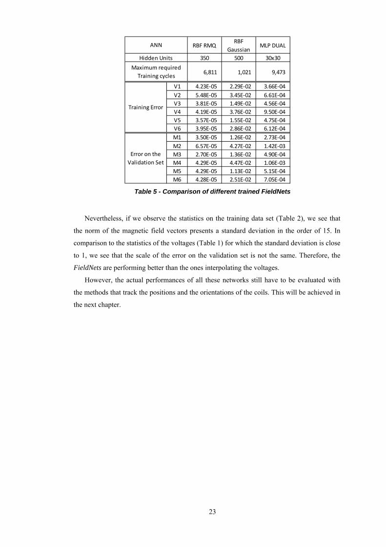
Table 5 - Comparison of different trained FieldNets ....................................................... 23 

Table 6 - Distances between coils using the VoltNets ..................................................... 38 

Table 7 - Distances between coils using the FieldNets .................................................... 43 

Table 8 - Intended local positions of the coils on the woodblock .................................... 49 

Table 9 - Mean of the optimized distances ...................................................................... 58 

 

1

Chapter 1 Introduction

Speech Synthesis has now become quite a common thing in our lives. The reader will

probably remember the hologram in the first Star Wars trilogy when the hero receives a

message and that the face expression is very accurate. However, at this time, the hologram

was just a pre recorded movie with some post processing effects to give the impression that

the person is not in the same place. There is still not a device that is capable of reproducing

the facial expressions for any spoken sentence. In order to do that, one must know all the

movements of the jaw, the tongue and the lips. There are some ways to do that, by using

optical devices, but this is not adequate to study articulography movements inside the mouth,

which is quite important for all the applications it allows (speech training for deaf people,

communication in noisy environments where microphones are unusable,...). Fortunately,

other means of recording these movements inside and outside the vocal tract have been

developed. They rely on an inductive measuring principle.

1.1 Electromagnetic Articulography

Electromagnetic transmitters driven by alternating current produce an inhomogeneous

alternating magnetic field. When a receiving coil sensor is placed in this field, an alternating

voltage is induced. Given the distance from the transmitter and the orientation of the sensor

relative to the transmitter, we may calculate the amplitude of the voltage that is induced

between the two ends of the sensor coil. A simple approach to explain these properties is to

use the dipole model which describes the magnetic flux density to be inversely proportional

to the cube of the distance from the transmitter. The induced voltage also depends on the

orientation of the sensor, so that it is proportional to the scalar product between the magnetic

field vector and the unit vector that describes the orientation of the sensor.

Therefore, given the position and orientation of the coils relative to those of the

transmitter, there is a simple way to calculate accurately the voltages which we expect to be

induced. However, this function that provides the amplitude of the voltage given the position

and the orientation of the sensor is not linear, and there is no simple way to invert it. Thus,

inferring the state of the coil in the magnetic field from measurements of the induced voltage

is not direct. In order to find positions and orientations of the sensor coil while the only data

2

that can be observed are the voltages, one needs to use iterative non-linear optimization

algorithms. Those methods aim to find an optimum state that minimizes the error between

the measured voltage and the voltage that is predicted at this position and this orientation.

The best outcome happens when the error is null, which means that the algorithm has ended

up with a state that is an antecedent of the measured voltage (though this does not

necessarily mean this is the only solution). In practice, the algorithm may find a locally

optimum solution and fail to converge on the globally best solution.

As already mentioned (and described more accurately in section 1.2.1), the relationship

between the state of the coil and the voltage is highly non-linear, which increases the

difficulty of predicting the state given the voltage. The voltage varies in a one-dimensional

space while the coil has 5 degrees of freedom, 3 Cartesian coordinates and 2 angles.

Therefore, one transmitter alone does not provide enough information to locate the sensor.

Many positions around the transmitter can be associated with the same voltage amplitude.

This problem can be solved by using several transmitters set at strategic positions. The AG-

500, described in section 1.2, uses 6 transmitters, and so to estimate sensors’ positions and

orientations, we essentially have 6 equations in 5 unknown variables to allow a 3

dimensional localization.

3

1.2 The AG500 Electro-Magnetic Articulography system

Figure 1 - The AG-500 device

(Photo from (Carstens))

The AG500 (Figure 1) is the most developed 3 dimensional Electro Magnetic

Articulography (EMA) system, and there is no other technology available that is fully

comparable in capabilities with this device. It provides real time motion tracking in 5 degrees

of freedom, which are the 3 Cartesian coordinates and 2 orientation angles. The device

comprises a cube-shaped acrylic glass structure with six transmitter coils arranged

spherically such that the receiver coil axis is never perpendicular to more than one

transmitter at a time (there is a right angle between every pair of transmitters) (see Figure 2).

Each transmitter has a unique frequency, ranging from 7.5 to 13.75 kHz so that, using

frequency demodulation, one can measure the voltage induced in the sensor coil

corresponding to each transmitter separately (Zierdt, Kaburagi, Hoole, Honda, & Tillman,

2000).

4

Figure 2 - AG-500 Coordinate System & Positions of the transmitters (Extracted from (Kaburagi, Wakamiya, & Honda, 2005))

The voltages induced can be measured in up to 12 receiver coils at the same time. The

voltage measured at the sensors depends on the distance from the transmitter and the angle

between the axis of each transmitter and of each sensor. The general method to describe the

variation of the voltages is to use the dipole model which is described in section 1.2.1 below.

Given the measured voltages in each sensor, Cartesian and angular coordinates of each of

them are determined by solving a set of non-linear mathematical equations. Given the

magnetic field model or a state-to-voltage function, the expected amplitudes are computed

and compared to the measured ones. Then, the determination of the states of the sensors is

achieved with some optimization methods in order to minimize the error between the

measured voltages and the expected ones. The commonly used optimization methods are

Newton’s Method, or Leven-Marquardt’s Method.

1.2.1 The dipole model

In the original version of the AG-500 implemented by A. Zierdt (Zierdt, Hoole, &

Tillman, Development of a system for three-dimensional fleshpoint measurement of speech

movements, 1999), the relation between the state (Cartesian and angle coordinates) of the

sensor and the amplitudes of the induced voltages is defined with the dipole model. This

model describes the magnetic field induced by and around a magnetic dipole, which is a

device with a close circulation of electric current. According to this model, the magnetic

field vector is governed by the equation:

5

,4

3 .23

 

where:

is the magnetic field vector at the position defined by ,

is the permeability of free space,

is the dipole moment,

is the vector from the position of the dipole to the position of the sensor,

is the three-dimensional delta function ( 0, except at 0; 0; 0 ),

Then, if is the opening angle between axis of the field vector and that of the sensor, the

voltage signal is proportional to:

, , 

1 3  ²  

where is the magnetic latitude measured from the dipole axis (see Figure 3).

Figure 3 - Magnetic Latitude

1.2.2 Calibration

The system that uses the dipole model requires calibration to define the relationship

between the voltage amplitudes and the state of each sensor. The dipole model only defines a

relation of proportionality between those two domains and this still remains to be

determined. To track the sensors through the magnetic field, the absolute measured signal

strength is not important, but in order to run the position calculation algorithm, this

amplitude must be calibrated to the expected signals or this would result in an inaccurate

6

tracking. This calibration factor is usually estimated using a rotating disk with several

sensors (see (Carstens) for more details of this procedure).

1.3 The objectives

The AG-500 has been shown to work satisfactorily and is used in research. However,

there is room for improvement in the accuracy and the reliability of this device (Yanusova,

Green, & Mefferd, 2009). In fact, there are some positional errors that are unacceptable in

some localized regions of the measurement field. The dipole model, together with calibration

factors found using Autokal (see (Zierdt A. , EMA and the crux of calibration, August

2007)), may not match the true physical properties of the AG-500 system at the time of

recording voltages. Those inaccuracies will be illustrated in this project.

As a consequence, one might consider building a representation of the magnetic field

based on interpolation methods where voltage measurements are taken at many known

positions in the measurement field. Then, interpolation of these is used to give the voltages at

any given point. Such representations of the magnetic field can provide satisfactory results as

this was presented in (Kaburagi, Wakamiya, & Honda, 2005). However, while this solution

proved successful, it has several downsides. Placing 12 coils accurately at many known

locations and orientations is an expensive, not convenient and time-consuming method. It is

not conceivable that this would be used before every experiment.

A potential solution to the inaccuracies of the dipole model would be to obtain a

trainable model of the magnetic field that could be further optimized with new data sampled

in the measurement field of the AG-500. Ideally, the only data to be used to optimize the

trainable model would consist of the movements of several sensors that are fixed relative to

each other through the measurement space. Unlike the method implemented by T. Kaburagi

and al. (Kaburagi, Wakamiya, & Honda, 2005), this solution would be cheap and easy to

achieve. Only minimal effort would be required to record the voltages from the movements

of the sensor coils constrained by being fixed relative to each other. Those measurements

would constitute a new training data set. Although we would not know exactly where each

sensor coil is in the measurement field, this measured data set would carry the limited

information that their relative positions and orientations are fixed. Using this knowledge, the

trainable model would be further optimized on this data set using machine learning

algorithms to match the true magnetic field as closely as possible. In this project, we will use

the data from an experiment done with 4 coils. Those 4 coils were fixed on a block with

approximately known relative positions and orientations.

7

However, the critical success factor of the overall method described above is to have

confident knowledge about the relative positions and orientations of the coils fixed on a rigid

body. While the sensors could be glued with intended dispositions, there might be some

degrees of inaccuracy that would make the overall method fail. Therefore, one should refine

the knowledge of the relative arrangement. Improving the accuracy of this limited

information aimed at optimizing the trainable model would increase the chances of obtaining

satisfactory results with the overall method.

Having some solution to derive and refine the coils' arrangements while they are known

to be fixed relative to each other would also add another advantage to this overall calibration

procedure. When a human subject, who has been glued up with sensor coils, is speaking in

the measurement field of the AG-500, coils fixed behind his ears, on his forehead and on the

upper part of his jaw stay fixed relative to each other. Unlike a woodblock where it is

possible to accurately measure the relative positions and orientations of the sensors, there is

no easy and direct way of doing it with the coils glued on somebody’s head. Thus, a method

that could discover the relative arrangements of those coils would be valuable. In fact, the

limited training data used to further optimize the magnetic field model could be directly

recorded before any experiment with the AG-500 involving a human subject. The limited

knowledge would consist in the movements of coils glued on somebody’s head at positions

where they stay with the same relative arrangements (behind the ears, on the nose, on the

forehead...). These relative dispositions would be discovered from the measured data.

In this project, we tackle the problem of finding a trainable model of the magnetic field.

The feasibility of using other models based on regression techniques is tested and their

accuracies are compared. The performances will be first evaluated on separate validation

data sets, and then using the data from the constrained movement of the 4 coils fixed on a

rigid body. These 4 coils stay at the same relative distances from each other during the

experiment. Therefore, accurate models must track those coils satisfying these constraints.

To be useful, a trainable model of the magnetic field will be expected to perform at least as

well as the dipole model currently used with the AG-500.

Then, we focus on the constrained tracking problem of the block where 4 coils were

fixed, and investigate the tracking accuracy of the block. This work was based on the

assumption that the relative positions and orientation of the 4 coils were known.

Finally, we implement and evaluate some methods to discover the arrangement of the 4

sensors on the rigid body, given that the actual positions and orientations of the coils could

slightly differ from the intended ones.

8

Chapter 2 Background

2.1.1 An inaccurate field model

A good deal of research has been done on how to minimize the error between the

measured voltages and the estimated voltages. As this is a non-linear optimization problem,

estimating a sensor’s position and orientation requires using non-linear methods to invert the

function that predicts the voltage given the position and the orientation of the sensor.

The magnetic field is highly sensitive to any perturbation. Any metal in the area modifies

the pattern of the field, and its amplitude. Thus, researchers know that there could be some

errors modelling the field and that it must be improved. That is why the designers of the AG-

500 have implemented a calibration procedure which is advised to be performed before each

experiment to reduce error.

This might also suggest that the dipole model is not very adequate for this device.

Previous experiments have shown that using it can lead to considerable errors. In (Yanusova,

Green, & Mefferd, 2009), Y. Yunusova reports the errors in the estimated trajectories of

sensors that are moved through a circular trajectory. Given the measurements of the voltages,

these estimated trajectories are not perfect circles as there are supposed to be. There are

some explanations to that, apart from the potentially inaccurate dipole model. The magnetic

fields created by the six transmitters can interfere, probably because of the mutual induction

between the coils, which makes the actual magnetic field deviate from the theoretical one.

2.1.2 Correcting the magnetic field model

In (Zachmann, 1997), G. Zachmann deals with a way of correcting the estimation of the

sensor’s position to make up for the distortion of the magnetic field. He focused on an

algorithm that could compensate for the inaccuracy of the field model in a (2.4m)3-cave. He

measured the magnetic field induced in the cave at 144 points placed on a regular lattice.

Then, using these sampled data and an algorithm based on global scattered data

interpolation, he built a representation of the magnetic field model and obtained method to

track sensors with higher accuracy. Nevertheless, tracking the positions of a sensor in such

an environment has a different application to articulography. This is used to create Virtual

Reality, but this exploits the same underlying principles. G. Zachmann obtained some

9

improvement on the tracking accuracy, which suggested that the magnetic field model could

be improved. Nevertheless, given that the data points were measured in a (2.4m)3-cave, the

standards are not the same as for the AG-500 and an error of 2-5cm in tracking the sensor’s

positions is quite high compared to the average error of the current AG-500.

2.1.3 Building the magnetic field model from data

T. Kaburagi and al. (Kaburagi, Wakamiya, & Honda, 2005) commented on the potential

limitations of the dipole model representing the magnetic field of the AG-500. They

suggested changing the field model itself and utilized multivariate B-spline functions to

interpolate the magnetic field given some sampled data. They measured the induced signal in

a receiver sensor coil that was placed at the crossing points of a grid drawn to cover in a

cubic region. This signal was sampled along every Cartesian axis at every crossing point.

Given those sampled data points, they built a multivariate B-Spline representation of the

magnetic field to be used instead of the dipole model. The expected voltages were calculated

from the scalar product between the magnetic field vector and the unit vector that expresses

the direction of the axis of the receiver coil. They obtained a higher accuracy with this new

model than with the dipole model. The reader must be aware that some of the relative error

can also be caused by the magnetic field model. In fact, this error is calculated as the

difference between the measured receiver signal and the predicted one using the B-spline

representation of the magnetic field, and normalized by the received signal at the origin of

the coordinate system as the reference. Therefore, an erroneous predicted voltage can

increase the average error.

The work of T. Kaburagi and al. suggests investigating the representation of the

magnetic field with other models or methods, such as interpolation methods. This also

suggests that a new state-to-voltage function that predicts the voltages given the Cartesian

and angle coordinates of the sensors could improve the accuracy of the tracking procedure

given some sampled data. Using representations of the magnetic field that exploits regression

techniques and which can be further optimized given some new sampled data might improve

the overall position tracking system. The first step of this method would be to approximate

either the magnetic field produced by each transmitter, or the voltages induced from each

transmitter and to use those approximations to track the coils through the field. In a second

step, those functions to approximate either the magnetic field vector or the induced voltages

would be optimized in a data-driven way. One would expect to obtain an average error that is

at least as low as the average error that is obtained with the currently used representation

based on the dipole model.

10

2.2 Artificial Neural Networks

In modern Mathematics, much work on approximation exists but there is only a small

portion of it that is interesting for the problem of improving the tracking accuracy of the

coils through the magnetic field. Given the evidence which indicates that the magnetic field

model presents a lack of accuracy and can be improved, a good approximation method for

this problem is the Artificial Neural Network (ANN). This is a model for regression where

the input vector is forward propagated through a succession of transformations. Each

transformation is symbolized by a neuron, which is also called a hidden-unit. In an ANN,

neurons can be connected to other ones. When two neurons have a directed connection, this

means that one of them computes a function that takes the output of the other neuron as an

input. Each neuron computes a function of a linear combination of input variables and/or

outputs of other neurons:

where:

is the output of the neuron ,

, 1, … , are an input variables or the outputs of other neurons,

, 1, … , are weighting coefficients,

is the function computed by the neuron ,

is the total number of inputs of the neuron .

ANNs are represented by graphical networks as in Figure 4. The function h is called the

activation function and defines the type of the ANN. In this problem, we have only used

feed-forward ANNs, which means that there is no closed directed cycles in the graphical

representation of the networks, and which ensures that the outputs are deterministic functions

of the inputs. Neurons can be classified in hidden layers. Then, every neuron computes a

function of the outputs of the neurons that belong to the hidden layer immediately below,

which creates a hierarchy in the hidden layers.

11

Figure 4 - Artificial Neural Network Diagram www.odec.ca/projects/2007/stag7m2/images

There has been a huge number of studies regarding feed-forward networks and their

potential to approximate arbitrary functions of finite number of real variables. It has be

proven (Cybenko, 1989, p. 308) that every bounded continuous function can be

approximated with arbitrarily small error by a network with one hidden layer and that any

continuous function can be approximated on a compact input domain to arbitrary accuracy

by a network with two hidden layers. Neural Networks are therefore said to be universal

approximators.

2.2.1 Analysis of several neural networks: Scattered Data Interpolation

There exist several sorts of ANNs, and all of them have different properties that make

them suitable for one modelling problem or another. The type of the ANN is defined by the

basis function that is symbolized by the hidden neurons. Common activation functions for a

hidden unit are either sigmoid function (logistic function, arctan...), or Radial-Basis-

Functions (RBF) (Gaussian functions, Multi Quadrics function...). The first ones implement

one kind of ANNs called Multi-Layered Perceptrons (MLP), and the latter define another

type of ANNs which are the RBF networks. The ANNs cited above have been shown to be

universal approximators given some conditions (see (Park & Sandberg, Universal

Approximation Using Radial-Basis-Function Networks, 1991), (Park & Sandberg,

Approximation and Radial-Basis-Function Networks, 1993) and (Cybenko, 1989)).

The Radial Basis function method has been shown to produce high quality solutions in

terms of accuracy to the problem of multivariate scattered data interpolation (Lazzaro &

Montefusco, 2002). However, this method has been associated with very high computational

12

cost, as compared to alternative methods such as finite element or multivariate spline

interpolation, and also a high computational cost for the training. The Radial Basis Function

networks are also highly sensitive to noise.

MLP networks have also been proven to be universal approximators, given enough

hidden units and hidden layers. They can also be costly computationally to train and to use if

there are several hidden layers.

We also considered another machine learning technique for this problem. Gaussian

Processes are usually highly accurate, efficient and easier to train. However, they require

storing all the training data points and the values of the kernels on these training data points,

which is not appropriate to large scattered data interpolation problems, such as encountered

in this study.

13

Chapter 3 Training Neural Networks to use with the AG-500

3.1 Creating the data sets

In order to train Neural Networks, we required a data set that captures the relationship

between the state (position and orientation) of the sensors and some other values that are

used to track the sensor in the field. In our case, those values were either the six voltages

induced in the coils by each transmitter, or the six magnetic field vectors produced by each

transmitter. Knowing that the recommended measurement volume is limited to a sphere with

a radius of 150 mm that is centred in the AG-500 cube, we have restricted our data points to

this area. Therefore, the data set should describe a reasonably large subset of these positions

and orientations of the coils throughout this sphere, which makes a 5-dimensional input

space. All data points were created in the following way: a radius ρ and two angles α and β

were sampled using a uniform distribution over the intervals [0; 150], [0; 2π] and [0; π]

respectively, in order to represent the point in a spherical coordinate system (see Figure 5).

Figure 5 - Spherical Coordinate System

Then, those three parameters were converted to the corresponding Cartesian coordinates.

The two angles θ and representing the orientation of the coil were also sampled from

14

uniform distributions over the interval [0; 2π]. Then, depending on the purpose of the neural

network, the target values were computed using one of the following methods.

Data set to interpolate the voltages

For the neural networks that map from the state of the coils to the voltages induced by

the six transmitters and which we will refer to as the VoltNets, the target values of every

input data point were computed using the calcamps function of the TAPADM toolbox

(Zierdt A. , The 3D-EMA Page). This function takes the state of the coil as input, changes

those coordinates to make them correspond to the local coordinate systems of each of the six

transmitters. Then it computes the magnetic field vector produced by each of the six

transmitters at the position of the coil. The output voltages are proportional to the scalar

product between this magnetic field vector and the unit vector that describes the orientation

of the coil in the coordinate system of the corresponding transmitter.

, , , , , , , , ,  

Data set to interpolate the magnetic field vector

For the neural networks that maps from the state of the coils to the magnetic field vector

and which we will refer to as the FieldNets, a modified version of the calcamps function that

directly outputs the magnetic field vector corresponding to every transmitter was used.

, , , , , , ,  

Using the two functions described above, a training data set of 100,000 samples and a

validation data set of 1,000 samples were created.

In the volume where the points were sampled, the voltages and the magnetic field vector

have the following characteristics:

Voltages V1 V2 V3 V4 V5 V6

Training set

Mean -0.004 0.001 -0.002 0.007 -0.002 0.005 Min -5.17 -7.83 -5.05 -8.46 -5.28 -7.82 Max 5.12 7.91 5.21 8.19 5.55 8.25

St. dev 0.764 1.041 0.654 1.123 0.768 0.944

Table 1 - Training Data Set for the VoltNets

15

Magnetic field

Training set Mean 30.02 42.96 28.17 44.89 28.42 42.21

St. dev 17.66 21.81 14.12 25.16 14.29 20.67

Table 2 - Training Data Set for the FieldNets

The target values of these data sets are not noisy; but determined by a function that uses

the dipole model. Even though the field model is supposed to be unknown in this problem,

creating the data sets in this way ensures that increasing the number of data points will not

have a negative effect on the trainings of the neural networks with respect to the accuracy.

However, this will add more constraints and will make the training more costly

computationally.

In order to evaluate the representation power of different VoltNets and FieldNets, the

data sets were restricted to a line with 1,000 training points, then a plane with 10,000 points.

Those intermediate steps revealed that thousands of training cycles were required before the

networks gave satisfactory results regarding the error on the validation sets. These pilot

experiments also highlighted the need to normalize the input data in order to restrict the

range of all inputs from -1 to 1 for the positions, and from 0 to 1 for the angles.

3.2 Methods to train the networks

The two functions which we want to represent using either the VoltNets or the FieldNets

and to compare are two non-linear functions. We had to run optimization algorithms to

approximate these functions with the corresponding networks. All computations have been

done using Matlab®. The networks and their optimizations have been achieved using the

Netlab toolbox (Nabney) which had to be modified to implement other kinds of networks

such as Radial-Basis-Function networks with Reverse Hardy’s Multiquadrics or dual hidden

layers Multi-Layered Perceptrons. All Networks have been optimized using the Scaled

Conjugate Gradient algorithm (Møller, 1993) which is already implemented in Netlab. This

algorithm is a variation of a conjugate gradient method that uses a Levenberg-Marquardt

(Kelley, 1999) approach in order to scale the step size instead of running a line-search

algorithm at each step. The scale bounds had been left to their default values set in Netlab

(10 10 ).

Given the large amount of data points in the training set, running the scaled conjugate

gradient algorithm as it has been implemented in Netlab gave rise to memory problems with

Matlab®. Therefore, the computation of the weights’ gradients using the back-propagation

16

algorithm had to be slightly modified in order to process the smallest matrices and vectors as

possible.

The representation power of a single hidden layer MLP might not be sufficient to this

problem. In order to assess these limits, the Netlab toolbox has been enhanced with a set of

Matlab® script to utilize dual hidden-layered MLPs (some of the scripts are provided in the

appendix). Those scripts are based on the original ones in Netlab and use the Back-

Propagation algorithm that is described in (Bishop, 2007, pp. 241-249). While the

representation power of dual hidden-layered MLPs is higher than for the single hidden-

layered MLPs, the computational cost is also much more significant. The amount of

weighting parameters is much more important as there is a weighting parameter for every

connection between the neurons of the first hidden layer and the neurons of the second

hidden layer. For instance, if the first hidden layer has n neurons and the second hidden layer

m neurons, there are (n x m) weighting parameters to represent the relationship between the

first and the second hidden layers.

In the original Netlab package, the Radial Basis Function networks can be defined with

the one of the following three hidden unit activation functions:

Gaussian Function: ²²

Thin Plate Spline function: ²log 

Polyharmonic Spline Function of 4th order: log 

Only the Gaussian functions have shown to be potentially able to interpolate the field

vector or the voltages. In fact, the voltages and the amplitude of the magnetic field vector

decrease with the distance from the transmitter. Therefore, the thin plate Spine functions and

the Polyharmonic Spline Function of 4th order are not adequate for this problem. However,

given this remark, we wanted to assess another type of Radial Basis Functions called the

Reverse Hardy’s Multi-Quadrics (RMQ) functions. Those functions are a close variant of the

Hardy’s Multi-Quadrics function. According to the comparison of some scattered data

interpolation methods in (Franke, 1982), those radial basis functions are one of the most

popular scattered data approximation methods. They were also tested in (Gorinevsky &

Connolly, 1994) and presented satisfactory results and high accuracy compared to the other

scattered data approximation methods. The form of those radial basis functions is as follows:

1 

17

where d is a scale parameter that has the same role as the standard deviation in a Gaussian

radial-basis function, and represents the norm of the position vector. When those

functions are incorporated in a neural network, the output of a hidden neuron which applies

this function is the following:

1 

where denotes the centre of the radial-basis function of the ith hidden unit, denotes the

input vector that is forward propagated through the neural network. In order to optimize a

RBF network with Reverse RMQ functions, the scripts in Netlab had to be adapted. The

main modification was done in the rbfbkp script, where the components of the gradient of the

network with respect to the parameters had to be implemented. The following derivatives

were used:

.  

.  

The details of the scripts can be found in the appendix.

3.3 Selection of Neural Networks

In order to obtain the best accuracy to track the coils in the AG-500, one needs to select

the neural networks that ensure the lowest error on a validation set as possible. The training

data that were utilized to train the networks are supposed to be non-noisy, given the fact that

they were sampled from the magnetic field model itself. Therefore, the error on the training

data set should express the accuracy of the neural network with a relatively high fidelity.

However, the performances of the different networks were assessed on the validation set

which contains 1,000 data points.

The relationship between the state of the coils and the voltages is highly non-linear and

the results of our pilot experiments lead us to define a VoltNet for every transmitter. Thus,

each VoltNet takes 5 variables as input and outputs one value. In fact, in the AG-500

measurement field, only the central region is used. The coils are never placed in the corners

of the acrylic cube. The relative location of this part of the measurement field is different for

every transmitter. It depends on the position and the orientation of the corresponding

18

transmitter relatively to the AG-500. Therefore, the magnetic field in this central region of

the AG-500 is different for every transmitter. This choice of defining one VoltNet for every

transmitter is justified in section 3.3.1.

Regarding the interpolation of the magnetic field itself, the FieldNets were also defined

in a similar way as for the voltages. Each FieldNet takes 3 variables as inputs which are the 3

Cartesian coordinates, and outputs the 3 Cartesian coordinates that represent the magnetic

field vector.

Given those settings, several types of networks were trained on the two data sets

described in section 3.1, and their performances were compared.

3.3.1 Function Complexity

The complexity of the function that we want to interpolate given the training data set has

been investigated. As this was previously described, the amplitudes of the voltages depend

on the position of the sensor relative to the transmitter, but also on the angle between the axis

of the coil and the one of the transmitter. Given the model used to represent the positions and

the orientations of the coils, there are 5 degrees of freedom: 3 Cartesian coordinates and 2

angles. In order to assess the difficulty to interpolate voltages, the same type of VoltNet was

trained with different training data sets containing the same number of data points. The first

data set contains data points that all have the same orientation, i.e. all the data points have

the orientation angles θ and φ set to 0°. The second data set contains the same amount of data

points but with θ varying and φ fixed and set to 0°. The third data set still has the same

number of data points but both θ and φ vary, as this is described in section 3.1. The results

are presented in Table 3. Figure 6 to Figure 8 represent the logarithm of the training error as

a function of the training cycles for each of the alternative data sets described above. Each

figure plots the logarithm of the training error of every of the 6 networks.

19

Table 3 - Comparison of the complexity of the state-to-voltage function

Figure 6 - Log of the training Error with the angles fixed to 0°

Cartesian Coordinates with 

fixed angles

Cartesian Coordinates with one angle varying

Cartesian Coordinates with 2 angles varying

1,952 14,197 34,500

V1 1.87E‐05 3.53E‐04 3.49E‐03V2 1.87E‐05 3.62E‐04 6.47E‐03V3 1.02E‐05 3.92E‐04 3.58E‐03V4 8.02E‐06 4.09E‐04 7.24E‐03V5 1.53E‐05 2.22E‐04 2.28E‐03V6 1.89E‐05 5.87E‐04 7.53E‐03V1 1.63E‐05 3.74E‐04 4.31E‐03V2 9.56E‐06 4.21E‐04 7.15E‐03V3 7.60E‐06 4.76E‐04 3.61E‐03V4 1.62E‐05 4.24E‐04 7.47E‐03V5 1.59E‐05 2.22E‐04 2.46E‐03V6 1.40E‐05 6.19E‐04 8.97E‐03

Average Error on the Validation Set (Volt)

Training Data Set

Maximum required Training cycles

Average Training Error (Volt)

20

Figure 7 - Log of the training Error with theta varying and phi fixed to 0°

Figure 8 - Log of the training Error with 5 degrees of freedom

The results show that the angles add some significant difficulty in interpolating the

function. If the input data had only 3 degrees of freedom, the problem would be much

simpler. Furthermore, the cost to train the function would be much more reduced since the

space from where to sample is only 3-dimensional instead of 5-dimensional. When one

degree of freedom is added, i.e. when one angle varies, the complexity of the state-to-voltage

function increases significantly, and training a network with those data is much more costly.

21

Therefore, this comparison justifies why it has been chosen to train one network for every

transmitter.

First, this reduced the complexity of the error function which then depends on one

voltage only. Second, this simplified the training process. In fact, the amount of training

cycles required to optimize every network with the data set described in section 3.1 was

above 10,000. Therefore, this required up to one week to train one type of network on the

data set. Every network was trained independently on computers with a capacities equalled

to or higher than a Dell OptiPlex 745 Desktop with 2GB of RAM. Those computational

requirements were ones of the main problems encountered through this project.

This comparison also suggests that this type of ANNs might be adequate for the

FieldNets. We will focus on this problem further in this chapter.

3.3.2 Training the VoltNets

The first aim of this project was to assess the feasibility of interpolating the voltages with

the VoltNets. As stated in section 3.3.1, this problem was quite challenging because the 5

degrees of freedom of the input space made the function quite complex. Several types of

ANNs have been trained on the data set and their abilities to accurately represent the

function were evaluated on the validation data set. More effort has been put on the Multi-

Layered perceptrons for this particular function. After the pilot experiments, those ANNs

proved to be more adequate to interpolate the voltages. In fact, the radial-basis function

networks did not lead to satisfactory results while tested on the validation set. Moreover, as

this was presented in section 2.2.1, RBF networks were also highly costly to train, as this can

be observed from the maximum number of required training cycles before a local minimum

was reached. This can be noted in the results which are presented in Table 4 where the

performances on the validation set are compared.

22

3.3.3 Training the FieldNets

As suggested in (Kaburagi, Wakamiya, & Honda, 2005), the dipole model might not

match accurately the physical magnetic field in some regions of the space. In order to make

up for this inaccuracy, this is possible to interpolate the magnetic field vector in the region of

the space were one wants to track the sensors. Therefore, the potential representation of the

magnetic field vector by ANNs has been evaluated (see Table 5). While a VoltNet with 350

hidden units of Reverse hardy’s Multi-Quadrics radial basis function was not adequate, this

was not the case for the FieldNets. A Gaussian RBF FieldNet was also trained on the data

set. However, the potential of this network turned out to be limited as one can see in Table 5.

The training process was stopped after about 1,000 cycles and without giving as satisfactory

results as the other evaluated networks.

MLP MLP DUAL MLP DUAL MLP DUAL MLP DUAL RBF RMQ RBF RMQRBF 

Gaussian500 200x300 300x200 400x100 50x400 350 500 500

19,358 7,537 9,473 7,916 7,043 34,500 21,000 8,000

V1 6.63E‐04 1.11E‐04 1.44E‐04 1.48E‐04 1.15E‐04 3.49E‐03 2.31E‐03 1.46E‐01V2 9.06E‐04 1.57E‐04 2.15E‐04 2.60E‐04 1.41E‐04 6.47E‐03 5.31E‐03 3.42E‐01V3 6.53E‐04 1.53E‐04 1.87E‐04 2.62E‐04 2.66E‐04 3.58E‐03 3.72E‐03 1.35E‐01V4 6.81E‐04 1.44E‐04 1.78E‐04 2.03E‐04 1.90E‐04 7.24E‐03 5.96E‐03 3.99E‐01V5 4.71E‐04 2.23E‐04 1.43E‐04 1.68E‐04 1.80E‐04 2.28E‐03 2.29E‐03 9.65E‐02V6 7.49E‐04 1.45E‐04 2.03E‐04 2.30E‐04 1.90E‐04 7.53E‐03 6.25E‐03 3.35E‐01V1 8.16E‐04 1.20E‐04 1.41E‐04 1.98E‐04 1.23E‐04 4.31E‐03 2.71E‐03 1.63E‐01V2 8.63E‐04 1.98E‐04 2.34E‐04 2.21E‐04 1.47E‐04 7.15E‐03 5.46E‐03 3.06E‐01V3 6.59E‐04 1.49E‐04 1.78E‐04 2.55E‐04 2.86E‐04 3.61E‐03 3.91E‐03 1.35E‐01V4 5.82E‐04 1.47E‐04 1.97E‐04 2.08E‐04 2.39E‐04 7.47E‐03 7.24E‐03 4.27E‐01V5 3.60E‐04 2.49E‐04 1.32E‐04 1.44E‐04 1.89E‐04 2.46E‐03 2.38E‐03 8.86E‐02V6 9.74E‐04 1.52E‐04 2.38E‐04 2.78E‐04 2.19E‐04 8.97E‐03 7.39E‐03 3.29E‐01

ANN

Hidden Units

Maximum required Training cycles

Average Training Error 

(Volt)

Average Error on the 

Validation Set (Volt)

Table 4 - Comparison of different trained VoltNets

23

Table 5 - Comparison of different trained FieldNets

Nevertheless, if we observe the statistics on the training data set (Table 2), we see that

the norm of the magnetic field vectors presents a standard deviation in the order of 15. In

comparison to the statistics of the voltages (Table 1) for which the standard deviation is close

to 1, we see that the scale of the error on the validation set is not the same. Therefore, the

FieldNets are performing better than the ones interpolating the voltages.

However, the actual performances of all these networks still have to be evaluated with

the methods that track the positions and the orientations of the coils. This will be achieved in

the next chapter.

RBF RMQRBF 

GaussianMLP DUAL

350 500 30x30

6,811 1,021 9,473

V1 4.23E‐05 2.29E‐02 3.66E‐04V2 5.48E‐05 3.45E‐02 6.61E‐04V3 3.81E‐05 1.49E‐02 4.56E‐04V4 4.19E‐05 3.76E‐02 9.50E‐04V5 3.57E‐05 1.55E‐02 4.75E‐04V6 3.95E‐05 2.86E‐02 6.12E‐04M1 3.50E‐05 1.26E‐02 2.73E‐04M2 6.57E‐05 4.27E‐02 1.42E‐03M3 2.70E‐05 1.36E‐02 4.90E‐04M4 4.29E‐05 4.47E‐02 1.06E‐03M5 4.29E‐05 1.13E‐02 5.15E‐04M6 4.28E‐05 2.51E‐02 7.05E‐04

ANN

Hidden Units

Maximum required Training cycles

Training Error

Error on the Validation Set

24

Chapter 4 Accuracy Assessment

4.1 Tracking the coils in the magnetic field

To recapitulate, each transmitter induces a signal in each sensor which depends on the

position and the axis orientation of the coil relative to the transmitter. For each sensor, six

voltages are recorded in order to find the 5 variables that describe the state of the coil. This

makes a system of 6 equations with 5 unknown. Those equations are not linear so that the

solutions need to be computed numerically using some optimization algorithms. Several

methods have been implemented to track the coils in the magnetic fields: the Calcpos

program (Carstens software that comes with the AG-500), the TAPADM toolbox and an

unscented Kalman Filter approach.

The AG-500 is initially used with the Calcpos program (Carstens). This program uses a

standard Newton-method along with a Householder transformation in order to compute the

QR decomposition and to estimate the solution of this overdetermined linear equation set.

A. Zierdt developed a Matlab® toolbox called TAPADM (‘Three-dimensional

Articulographic Position and Align Determination with MATLAB’) as an open-source

alternative to the Calcpos program (Zierdt A. , The 3D-EMA Page). This toolbox can use

other optimization methods than the Newton algorithm, such as the Levenberg-Marquardt

algorithm.

K. Richmond (Geng, Richmond, Renals, & Turk, 2009) implemented another approach

to track the sensors in the magnetic field. He used an Unscented Kalman filtering algorithm.

4.2 Unscented Kalman Filtering

When the coils are moved through the magnetic field, the voltages are usually recorded

with a sampling rate of 200Hz. This makes a discrete-time movement with one sample every

0.005 second. Successive samples are strongly correlated, because they refer to close

positions and orientations of the sensor coils. This correlation can be used to track the coils.

25

4.2.1 Kalman Filtering

The Kalman filter is an efficient recursive filter that estimates the hidden state of a

dynamic system from noisy observation measurements. The Kalman Filter operates by

propagating the mean and the covariance of the state through time, using the mathematical

description of the dynamic system. It is based on a linear discrete-time system given as

follows:

State-update Equation:            

Measurement-update Equation:          

where:

is the hidden state at time k,

is the observation at time k,

is the state transition model which is applied to the previous hidden state

,

is the control-input model which is applied to the control vector ,

is the process noise which is assumed to be drawn from a zero mean

multivariate normal distribution with covariance ,

is the observation model which maps the true hidden state space into the

observed space,

is the observation noise which is assumed to be drawn from a zero mean

multivariate normal distribution with covariance ,

The noise processes are supposed to be uncorrelated, i.e.:

   

   

 0 

where is the Kronecker delta function, which means that 1 if , and

0 if . The Kalman filter is a recursive estimator as described in the equations

above. It uses the state from the previous time and the observation measurement at time k to

compute the estimate for the current state. It first estimates an a priori hidden state and

an a posteriori hidden state which are the expected value of the state at time k

conditioned on all the measurements before (but not including) time k and the expected

26

value of the state at time k conditioned on all the measurements up to and including time k,

respectively.

| , , … ,  

| , , … ,  

Given those two estimates, it also computes the covariance matrices of the a priori and

the a posterior estimation errors, noted respectively and .

 

 

One also needs to define the Kalman Filter gain which adjusts the importance given

to the new measurement in the a posterior estimation:

 

The initialization of the Kalman filter is achieved as follows:

 

 

Then, for each time step 1,2, … , ∞ , the algorithm is run as follows:

 

 

 

 

 

The above description of the algorithm is the general one. All the details can be found in

(Simon, 2006, pp. 123-148). The main flaw of this algorithm is that it relies on a strong

assumption: the state transition equation and the measurement equation are linear. Therefore,

this version of the Kalman filter cannot be applied to the problem of tracking the coils in the

magnetic field as the relation between the state of the coils (position and orientation) and the

measurement equation is non-linear. In order to make up for this linear assumption, one

needs to use a modified version of the original Kalman Filter.

27

4.2.2 Unscented Transform

Most non-trivial real-world systems are non-linear. The non-linearity can stem from the

state update equation or the measurement equation or both.

State-update Equation:     ,    

Measurement‐update Equation:                

The non-linear functions f and h cannot be applied to the covariance matrices. In order to

make up for these flaws, there exist at least two methods. The Extended Kalman Filter uses

matrices of partial derivatives of the functions. But it is difficult to implement and can only

be used with systems that are almost linear. For highly non-linear systems, the Unscented

Kalman Filter (UKF) has proven to be much more efficient and much more accurate. It uses

a deterministic sampling approach in order to propagate mean and covariance information

through the non-linear equations. This is known as the unscented transform. The sampled

points capture the posterior mean and covariance accurately to the 3rd order according to the

Taylor expansion. It was first developed by Simon J. Julier and Jeffrey K. Uhlmann (Julier &

Uhlmann, 1997) and further improved by Eric A. Wan and Rudolph Van der Merwe (Wan &

Van der Marwe, 2000).

The unscented transformation computes (2L+1) points, where L is the dimension of the

variable that needs to be propagated through a non-linear function. It starts from the

assumption that the mean and the covariance matrix are known. Using those, a matrix

of (2L+1) sigma vectors is calculated:

 

, 1, … ,  

, 1, … ,2  

 

1  

12

, 1, … ,2  

where:

28

is a scaling parameter,

, and are fixed parameters that are usually set to 10 , 2 and 0 respectively.

is the ith row of the matrix square root,

and are weighting parameters used to compute the mean and the

covariance respectively.

Those computed sigma points are propagated through the nonlinear function g which can

be the state and/or the measurement function:

Ζ χ , 0, … ,2  

And the mean and the covariance are approximated using the weighting parameters!

Ζ Ζ  

Ζ Ζ Ζ Ζ  

This transformation is used along with the Kalman Filter algorithm to form the

Unscented Kalman Filter. It first estimates the a priori state and the a priori measurement

given the sigma points computed with the vectors and matrices from the previous time k-1.

Then, it estimates the observation covariance matrix and the state-observation covariance

matrix to calculate the Kalman Gain matrix and achieve the measurement update step. The

complete algorithm is described below (see (Haykin, 2001, p. 232)):

Initialization:

and are initialized as with the linear Kalman Filter. Then the process noise

and measurement noise are added to the state vector:

 0 0  

0 00 00 0

 

For each time step 1,… ,∞ , the sigma points of the state augmented with

the process and measurement noises are computed as follows:

 

29

For each column 1,… ,2 1 of (L is the dimension of the augmented

state: ):

 

Time-update equation:

| , , 1, … ,2 1  

|  

| |  

Υ | | , 1, … ,2 1  

Υ |  

Measurement-update equations:

, Υ | Υ |  

, | Υ |  

, ,  

 

,  

This algorithm assumes that the process and the measurement equations are linear with

respect to the noise. One will see that this assumption is valid with the problem we are

focusing on in this study. The algorithm presented is the general form of the UKF. This can

be applied to the problem of tracking the coils in the magnetic field as this is presented in the

following section.

30

4.3 Unconstrained Tracking

The relationship between the state of the sensors and the amplitudes of the voltages that

are induced by the transmitters is non-linear. Therefore, in order to apply a Kalman filter to

track the coils through the magnetic field, one needs to use the Unscented Kalman filtering

algorithm. In fact, the update equation and the measurement equation are as follows:

Update-equation:

 

where are the three Cartesian coordinates and the 2 angle coordinates of the coil at time

, and is the process noise

Measurement equation:

 

φ

 

Where:

is the ith voltage measured on the coil at time ,

is the observation model,

is the observation noise which is assumed to be zero mean Gaussian

white noise

The reader can verify that the measurement equation is non-linear and requires using the

unscented version of the Kalman filter. In those equations, the state of the coil is set as the

hidden state variable, and the six voltages represent the measurements. Given this model and

the recorded voltages sampled at 200 Hz, the UKF can be run to track the movement and the

orientation of the coil. This model uses a fictitious process noise to represent the movement

of the coil. The time-update equation is linear and the state at time k equals the state at time

k-1 with addition of some process noise. This allows the filter to place more emphasis on the

measurements and ensures that the coil can move according to the measured voltages.

31

However, it is difficult to estimate the covariance of the process noise that will ensure an

accurate tracking process. If a system model has too much noise, this makes it difficult to

estimate its state and will end up with a higher tracking error because of the addition of some

random movements. But a too little noise will make the system more rigid and prevent it

from tracking the true movement of the coil, especially when the sensor is moving rapidly.

Therefore, the process noise covariance plays an important role in the tracking process.

Regarding the problem of tracking the coils in the AG-500, the state values

approximately vary from -150 mm to +150 mm for the Cartesian coordinates and from 0° to

360° for the angles. The 5 coordinates roughly vary through ranges of the same amplitude.

With regard to the problem of tracking each coil independently, a process noise covariance

of 0.5 has proven to be adequate, given that the speed of the coils is quite limited and that the

sampling rate is high enough. Concerning the measurement-update equation, the noise

covariance was set to 10-4 and expresses the error in measuring the amplitudes of the

voltages.

The three scaling parameters of the UKF, α, β and κ, have been set to fixed values

according to the description in (Van der Merwe & Wan, The square-root unscented Kalman

Filter for state and parameter-estimation, 2001). α determines the spread of the sigma points

around the a priori estimation of the state, β is used to incorporate prior knowledge of the

distribution of the state and κ is another scaling parameter. They have been set to the

following values:

1 

2 

0 

The model described above ignores the exogenous input .

This algorithm was implemented in Matlab® using the existing toolbox ReBEL-0.2.7

which was used under the Academic License (Van der Merwe & Wan, ReBEL, 2006). The

initial state covariance was set to 0.75  , and the initial state of the coils was set to the

values which were computed with the CalcPos program when the data were acquired. Given

those initial conditions and this model, the trajectories of the sensors were computed

independently.

32

4.4 Accuracy of the new field models

The different ANNs trained in sections 3.3.2 and 3.3.3 are aimed at interpolating either

the voltages (VoltNets), or the magnetic field vector (FieldNets). A first evaluation could be

done by comparing their performance on a validation set. However, the main purpose of

training those ANNs is to use them as a substitute for the dipole model to track the coils in

the AG-500 measurement field with at least the same accuracy.

In order to evaluate the performance of the ANNs and to compare them to the calcamps

function provided with the TAPADM toolbox, we used some data measured with 4 coils that

were moved in the AG-500 magnetic field. Those 4 coils were fixed on a woodblock so that

their relative positions and orientations remained constant. In particular, the distances

between the coils are constant. In this experiment, the block was first held relatively steady

in the measurement field. Then, in a second phase, this rigid body was rotated with a

backward and forward motion. The rotations had approximately the same amplitudes, but the

frequency of the rotations was increased with the time.

A “good” tracking method should calculate a trajectory for each coil that respects the

constraint of staying at the same distances from the other coils. The 4 coils were aligned on

the block with different orientation, as illustrated in Figure 9.

Figure 9 - Arrangement of the coils on the woodblock

Each coil was tracked independently using the UKF algorithm and the corresponding

recorded voltages. The UKF algorithm was run with every ANN that we want to assess, and

also with the calcamps function. Figure 10 shows the distance between the coils 3 and 4 as a

function of the time. While the coils are supposed to stay at the same distance, this figures

shows that there is some tracking error when the calcamps function is used. In fact, the

33

distance ranges approximately from 56 mm to 63 mm while it should remain fixed to a value

close to 60 mm.

Figure 10 - Distance between coils 3 & 4 tracked with the calcamps function

In the following paragraphs, the performances of the trained VoltNets and FieldNets are

evaluated using the distances between some of the coils on the woodblock. However, as

shown in Figure 9, the coil n° 2 was fixed with a different orientation from the other ones. Its

trajectory which was computed with the UKF and the observation functions (including the

calcamps function) presented some irregularities which could be justified with the different

orientation and which increased the standard deviation of the distances between this coil and

the others.

The 3-dimensional plots in Figure 11 illustrate the inaccurate tracking of this coil. They

represent a succession of 6 sampled images from the movement of the 4 coils.

34

35

Figure 11 - 3D Plot of the movements of the 4 coils

Figure 11 provides a succession of images sampled from the 3-dimensional movement of

the 4 coils tracked independently. In the first 3 images, the block starts rotating towards the

vertical position. When the vertical position has been reached, the second coil deviates from

the axis where the 3 others are aligned (images 4 and 5). Then, when the block rotates

backwards to the horizontal position, the coil n° 2 goes back to an aligned relative position

(image 6).

In order to show the inaccuracy of the field model, we focused on the root mean square

error between the measured voltages and the predicted ones using the calcamps function

(based on the dipole model). The RMS error as a function of the time is plotted for each of

the coils from Figure 12 to Figure 15.

36

Figure 12 - RMS error of the coil 1

Figure 13 - RMS error of the coil 2

37

Figure 14 - RMS error of the coil 3

Figure 15 - RMS error of the coil 4

One can observe that the RMS error for the coil 2 is at least twice higher than for the

other coils, which supports the hypothesis that there is still a “calibration” problem with the

field model, inducing higher error when the axis of the coils are getting closer to the vertical

axis.

38

4.4.1 Networks interpolating the voltages

Using the ANNs that were trained on the magnetic field, we ran the UKF algorithm to

track each coil independently. Then, the distances between some of the coils were analyzed

for every network. All the coils are fixed on the block. Therefore, when the coils are tracked

independently using one of those networks, the trajectories of the coils should respect this

constraint of moving the coils at the same distance.

Unlike the second coil, we know that the trajectories of the coils 3 and 4 are tracked

coherently and with more satisfactory accuracy than the 2 others when the dipole model is

used. In fact, they presented the smallest RMS error during this experiment (see Figure 12 to

Figure 15). A good network used to track the coils independently should keep the distance

between those 2 coils almost as constant as when the dipole model is used. One can observe

in Table 6 that even the dipole model presents some inaccuracies and that the standard

deviation of the distances between the coils 1 and 3, or the coils 3 and 4 is higher than 1 mm.

Once again, this supports the idea of obtaining a new model for the magnetic field. However,

Table 6 also shows that the VoltNets do not provide accurate tracking of the coil. Except for

the Dual hidden-layered MLP networks with 50x400 hidden units, the standard deviation of

the distances between two confident coils is superior to 2.5 mm, and the distances can

deviate by more than 20 mm from their actual values.

Table 6 - Distances between coils using the VoltNets

In order to visualize those results, the distances between the coils 3 and 4 are plotted in

Figure 16. This demonstrates that interpolating the voltages using those types of VoltNets

does not provide satisfactory results. The computed distances with the coils tracked using

those networks present many more spikes with higher amplitudes than with the dipole

calcamps MLPMLP DUAL

MLP DUAL

MLP DUAL

MLP DUAL

RBF RMQ RBF RMQ

N.A. 500 200x300 300x200 400x100 50x400 350 500min 4.71 3.73 6.79 2.31 4.81 1.76 8.87 1.61max 73.88 51.78 42.27 74.74 62.07 521.66 351.99 283.21mean 20.09 30.68 22.30 20.94 22.95 30.39 149.76 106.14st. Dev. 5.91 8.92 4.31 7.62 5.45 61.37 87.77 99.49min 41.51 37.60 36.49 42.91 43.71 53.54 28.76 28.44max 70.59 108.69 67.05 70.98 69.78 81.45 203.62 217.98mean 60.19 57.90 58.49 61.00 57.62 61.69 79.92 77.11st. Dev. 1.59 9.37 3.19 3.16 4.33 3.75 33.27 28.97min 54.91 41.25 49.82 53.84 43.37 52.02 30.21 17.46max 62.74 68.86 70.73 69.15 67.78 63.90 81.05 142.45mean 59.90 61.31 57.89 61.50 60.86 59.32 59.86 65.00st. Dev. 1.20 5.07 2.53 2.52 4.93 1.76 8.03 17.09

ANN

Hidden Units

coil3‐coil4

coil1‐coil3

coil1‐coil2

39

model. Therefore, we can conclude that the voltages cannot be accurately interpolated using

neural networks that are trainable with Matlab® and a training data set of 100,000 points.

Single hidden-layered MLP Network with 500 hidden units

Dual hidden-layered MLP Network with 200x300 hidden units

40

Dual hidden-layered MLP Network with 300x200 hidden units

Dual hidden-layered MLP Network with 400x100 hidden units

41

Dual hidden-layered MLP Network with 50x400 hidden units

RMQ RBF Network with 350 hidden units

42

RMQ RBF Network with 500 hidden units

Figure 16 - Distance between coils 3 & 4 – VoltNets

4.4.2 Networks interpolating the magnetic field

In the same way as we evaluated the VoltNets, we used FieldNets to track the 4 sensors

of the woodblock. The UKF algorithm was run with each of the ANNs. The results of these

experiments (see Table 7) show that those FieldNets perform as well as the dipole model.

The standard deviations of the distances between the coils 1 and 3, or the coils 3 and 4 are of

the same order as the standard deviations obtained with the calcamps functions. The

distances also range by the same amplitudes and the difference between the means of the

distances is inferior to 0.3 mm.

43

Table 7 - Distances between coils using the FieldNets

Those results show that the three FieldNets provide as accurate results as the calcamps

function. Even the Gaussian Radial Basis Function network, which was not performing with

the same accuracy on the validation set after the training, gives as satisfactory results as the

other networks for this experiment. In order to visualize the performance, the distance

between the coils 3 and 4 as a function of the time is provided below for each of the

networks.

RMQ RBF Network with 350 hidden units

calcamps RBF RMQRBF 

GaussianMLP DUAL

N.A. 350 500 30x30min 4.71 4.69 4.63 4.85max 73.88 72.41 75.89 74.27mean 20.09 20.07 19.84 20.03st. Dev. 5.91 5.82 6.16 5.97min 41.51 41.42 41.54 41.81max 70.59 70.78 72.42 70.78mean 60.19 60.20 60.00 60.23st. Dev. 1.59 1.61 1.76 1.63min 54.91 54.92 55.00 54.84max 62.74 62.75 63.17 62.94mean 59.90 59.91 60.04 59.91st. Dev. 1.20 1.20 1.18 1.23

ANN

Hidden Units

coil1‐coil2

coil1‐coil3

coil3‐coil4

44

Gaussian RBF Network with 500 hidden units

Dual hidden-layered MLP Network with 30x30 hidden units

Figure 17 - Distance between coils 3 & 4 - FieldNets

45

Those plots show that these networks provide results that are similar to the ones obtained

with the calcamps function. The Reverse hardy’s Multi-Quadrics network with 350 hidden

neurons computed a distance between the coils 3 and 4 that almost perfectly matches the

distance computed with the dipole model. The distances tracked with the two other networks

are also quite similar to the ones tracked with the calcamps function. Therefore, this provides

evidence that the magnetic field vector can be interpolated with a trainable model.

46

Chapter 5 Optimizing the field model

5.1 A constrained tracking problem

In order to optimize the field model initialized from the dipole model (as in Chapter 3 ),

some more data are necessary so that the field model can be adjusted. Some perturbations

due to the environment can slightly modify the magnetic field and therefore add some error

to the tracking process. The aim of the field model optimization is to obtain a function that is

closer to the actual magnetic field or the actual amplitude of the voltages to make up for

those perturbations. The only way of doing this kind of optimization is to measure some data

to get some knowledge about the actual magnetic field. One way of doing this is to record

the voltages with some sensors moving through the field. However, in order to get data that

provide information about the relationship between the state of the coils and the measured

voltages, one needs to have some precise knowledge about the position and the orientation of

some coils.

In this project, we propose an alternative approach based on a constrained tracking

problem. Several sensors were fixed relative to each other on a rigid block and moved

through the measurement space. Thus, the positions and the orientations of the coils relative

to each others remain fixed although none of the trajectories is known accurately. Working

out how best to exploit this knowledge of the fixed distances is not trivial. For example, if 2

coils are fixed relative to each other at a distance D, knowing the state of one of them does

not define the position of the second coil. The latter could be anywhere on the surface of the

sphere of a radius D, centred at the first coil. Adding the information of the tracked trajectory

of the second coil does not even define exactly its position given that the tracked one could

even not be on the surface of this sphere. Given that we do not know exactly the position of

either of the 2 coils, the difficulty is even higher.

To tackle this problem, we implement a solution which is based on an Unscented

Kalman Filtering algorithm . We use the data from the woodblock with the 4 coils. Then,

assuming that the coils 1, 3 and 4 are reliable enough (see section 4.4), the constraints

between the sensors are used along with an Unscented Kalman Filter to enhance the

accuracy of the tracking process.

47

The implementation of such a method is different from the one that was used to track the

coils independently. The state variable is no longer the 5-dimensional state of the coil but a

6-dimensional vector that describes the state of the whole block onto which the coils have

been fixed. These six degrees of freedom are the 3 Cartesian coordinates and the 3

orientation angles of the block that have been chosen to be the Euler angles. Those angles, α,

β and γ, represent the rotation around the z-axis, the line of nodes axis and the new Z-axis

respectively (see Figure 18). The line of nodes axis is the intersection of the xy plane before

rotation of the coordinate system, and the plane XY after the rotation.

Figure 18 - Euler Angles (Figure from http://en.wikipedia.org/wiki/Euler_angles)

The state transition model is still set with the identity matrix, and the transition equation

includes some process noise with a zero mean multivariate distribution, as described below:

 

where are the coordinates of the block at time , and is the process noise

The measurement equation is more different from the previous model that was used

to track the coils independently. The measurements are all the voltages recorded with every

coil that has been fixed on the block. Knowing with some confidence the positions and the

orientations of every coil on the rigid body, the state of the block at time can be linked to

48

the whole set of the recorded voltages, which exploits the knowledge of the constraints

between the coils. The measurements also include some observation noise, as described

below:

,

,

,

,

 

where:

, is the jth voltage measured on the ith coil at time , where is the

number of coils fixed on the block,

is the observation model based on the position of the sensors relative

to the position of the block, and the field model,

is the observation noise which is assumed to be zero mean Gaussian

white noise.

The observation model uses either the dipole model, or one of the FieldNets

trained in section 3.3.3. Given the arrangement of the coils on the block, the position and the

orientation of each of them can be inferred from the state of the block, and then linked to the

voltages. A more precise description of this is provided in the following section.

5.1.1 Tracking the woodblock in the field

The coils on the woodblock were placed with different orientations and different

distances. Figure 19 illustrates the relative positions of the coils and shows how the local

coordinate was chosen to link the 6 coordinates of the block to the coordinates of each of the

coils. The 3rd coil was chosen to be the origin of the local coordinate system.

49

Figure 19 - Woodblock with 4 coils and the local coordinate system

The intended positions of the coils in the local coordinate system are summarized in

Table 8.

Coil  X (mm)  Y (mm)  Z (mm)  θ (degree)  φ (degree) 1  0 ‐80 0 0 0 2  0 ‐60 0 ‐90 0 3  0 0 0 0 0 4  0 60 0 180 0 

Table 8 - Intended local positions of the coils on the woodblock

Given these local coordinates of the coils and the global coordinates of the woodblock, it

is then possible to compute the global coordinates for every coil. This local coordinate

system is obtained from the global coordinate system with a composition of rotations, which

have been chosen to be the Euler rotations. Given the three Euler angles, the matrix

representations of the rotations were multiplied with the vectors of the local coordinates of

each coil to obtain the positions in the global coordinate system. The orientation of each coil

was converted into three Cartesian coordinates to allow the multiplication with the rotation

matrices. The three Euler rotations were represented as follows:

cos  sin  0sin  cos  00 0 1

 

1 0 00 cos  sin 0 sin  cos 

 

50

cos  sin  0sin  cos  00 0 1

 

where:

Rz is the rotation around z-axis the global coordinate system,

Rn is the rotation around the line of node,

RZ’ is the rotation around the Z-axis of the rotated frame.

The coordinates of each coil in the global coordinate system are computed as follows:

       

where the coordinates in the local frame are in capital letters, the ones in the global

coordinate system in small letters, and where the variables with a subscript “o” denote the

Cartesian representation of the unit vector of the orientation.

Given the positions and orientations in the global coordinate system, the corresponding

voltages can be calculated with either one of the FieldNets, or the calcamps function from

the TAPADM toolbox. This relationship between the state of the woodblock and the

measured voltages constitutes the observation model used in the unscented Kalman filter.

Given that the Euler angles are defined modulo 2 , we had to use the option available in

the Rebel toolbox to deal with angle discontinuities. This was set by adding the following

line of code: model.stateAngleCompIdxVec = [4 5 6];

This line declares the parameters number 4, 5 and 6 as angles before the Inference data

structure is created in Rebel.

5.1.2 Several alternatives to track the woodblock

Previous analysis (section 4.4) has shown that some parts of the tracked trajectory of the

coil 2 on the woodblock present some irregularities. When the axis of this sensor is close to

the z-axis of the global coordinate system, the tracked position of this coil deviates distinctly

from its actual one that we can approximately infer from the positions of the 3 other sensors.

Therefore, when the Unscented Kalman filtering algorithm is run to track the trajectory of

the woodblock, this coil gives erroneous information that might add some error to the

51

tracked movement. In order to gauge the impact on the tracking process, we implemented

two versions of the measurement equation in the UKF. In a first experiment, the 24 voltages

that correspond to the 4 coils were used to define the observations for the model, and in a

second experiment, the coil n°2 was excluded from the model to use only the 3 other coils. In

the latter version, only the 18 voltages corresponding to the exploited coils were taken into

account.

Then, we used the trajectories of the 4 coils tracked independently with the calcamps

function to do further analysis. Given the tracked positions and orientations of the block, we

applied the opposite rotations and translations to the independent trajectories of the 4 coils in

order to observe their local movement in the local frame of the woodblock. This was done

for both the experiment using the 18 voltages and the one using the 24 voltages. The plots in

Figure 20 to Figure 25 represent the local Cartesian coordinates of the coils in the frame of

the woodblock.

52

Figure 20 - Local positions on X-axis - Block tracked with 3 coils

Figure 21 - Local positions on Y-axis - Block tracked with 3 coils

53

Figure 22 - Local positions on Z-axis - Block tracked with 3 coils

Figure 23 - Local positions on X-axis - Block tracked with 4 coils

54

Figure 24 - Local positions on Y-axis - Block tracked with 4 coils

Figure 25 - Local positions on Z-axis - Block tracked with 4 coils

The coils were stuck on the woodblock with the intended positions and orientations

given in Table 8. There might be some slight deviations from those which could be about 1

55

mm and a couple of degrees. This could be the cause of a small difference from the 0-axis

that one can observe in Figures Figure 20, Figure 22, Figure 23 and Figure 25. However, this

small error should be in the order of 1 mm for the Cartesian coordinates and 2 or 3 degrees

for the angles. Even if the tracked trajectories of the coils are not the actual ones, we know

that the local movements in the frame of the woodblock should stay around the intended

locations reported in Table 8. The positions of the coils in the local frame when the block

was tracked with 3 coils present a higher deviation from the intended values than when the

block was tracked with the whole set of coils. This can be observed distinctly with the X and

Z local coordinates. In Figure 22, the difference can be up to 10 mm on the Z-axis. The coil

4 stays around +5 mm on this axis, and the coil 1 around -5 mm, while both of them should

stay in the local XY plane. As a matter of fact, the remaining constraints when only 18

voltages are processed to infer the state of the woodblock are not sufficient. Given that there

are fewer constraints, the orientations of the main axis of the woodblock (which is the local

Y-axis) are tracked with lower precision. The calculated orientations of this axis differ from

the actual ones and the coils are no longer in the local XY plane, which explains this

difference in the positions on the Z-axis.

Therefore, the tracking algorithm that exploits the 24 voltages is more appropriate for

this problem, even if the trajectory of the second coil presents some irregularities. The

version of the constrained tracking is the one that has been retained.

5.2 An EM approach to optimize the tracking of the woodblock

The field model currently in use allows tracking the coils with an error which is below 1

mm. In order to expect any improvement of this model using measured data, one must utilize

reliable data so that the optimization of the model will not degenerate to nonsense. With the

solution of the constrained tracking, the relative positions and orientations of the coils must

be known with high confidence. However, the “theoretic” arrangement of the coils on the

woodblock might slightly differ from the actual ones. Given that these data are supposed to

be analyzed to optimize the field models, they must be precise and reliable for this purpose.

Therefore, the relative positions used need to be processed and optimized to make those new

limited training data as accurate as possible and to expect some improvement of the field

model.

56

5.2.1 Measuring the positions and orientations of the coils on the woodblock

There are many different ways to try to discover the relative positions of the coils on a

block. However, the difficulty to achieve this optimization is that each coil has 5 degrees of

freedom which, added to the 6 degrees of the freedom of the block, makes a challenging

number of unknowns. Therefore, in order to make up for this high dimensionality of the

space where the optimization is computed, one needs to either use more equations, either

keep some constraints. The first option would require more measures for the coils, which

means more voltages, and which is then not conceivable. The second option can be done by

assuming that we have some knowledge about the relative positions and orientations of the

coils. This presumably correct knowledge should be defined according to the problem.

Regarding the woodblock, there are different variables describing the states of the coils

on the woodblock that could be assumed to be known with a high confidence. Some others

can be potentially less confident, and these are the variables that we want to refine. On the

block, the coils are supposed to be perfectly aligned. Given the distances between the coils,

one can assume that this alignment is sufficiently correct. However, the distances could

present a small inaccuracy, and given that they are supposed to be utilized in the observation

model to track the whole block, their actual values should be known with high confidence.

In order to discover the distances, those were introduced as unknown in the Unscented

Kalman filtering algorithm, even if they are still parameters in the observation model. Doing

that, the tracking algorithm becomes an alternative version of the UKF, called the Joint

Unscented Kalman Filter. This version of the algorithm optimizes jointly the unknown

variables and parameters, i.e. it tracks the block and optimizes the distances used in the

observation model at the same time.

The difficulty that was encountered is that the distances are actually a function of the 3

Cartesian coordinates of the coils, which means that knowing the distances between the coils

does not give sufficient knowledge about their relative positions. A coil situated at a known

distance from another could be anywhere on the surface of the sphere centred on the second

coil with this distance as radius. Therefore, we had to assume that the coils were confidently

aligned on the block. Therefore, the distance was expressed by the position on the local Y-

axis (see Figure 19). The augmented state vector of the Joint Unscented Kalman Filter was

defined as follows:

57

 

where , , , , and describe the state of the woodblock as defined in section 5.1, and

, and describe the distances of the coils 1, 2 and 4 respectively, from the coil 3

which was chosen to be the origin of the local coordinate system. This augmented state

contains the distance parameters which are optimized jointly with the positions and

orientations of the block. In the observation model, the optimized distances were used as the

coordinates of those 3 coils on the local Y-axis.

The joint UKF was run on the same data set of the woodblock. The variance of the noise

corresponding to the distances was set to a small value (10-7), given that they are not

supposed to vary significantly. The results are reported in Figure 26.

58

Figure 26 - Optimization of the distances between the coils

Coil 1 to Coil 3 Coil 2 to Coil 3 Coil 3 to Coil 4

Mean distance (mm) 68.07 82.61 57.56

Table 9 - Mean of the optimized distances

This solution presented bad results. In fact, the coils are supposed to be fixed on the

woodblock at positions and orientations close to the intended ones (see Table 8) and should

not differ from them by more than 1 or 2 mm regarding the Cartesian coordinates. Therefore,

59

we wanted to assess if the problem was not a consequence of a bad tracking of the block.

Given the distances and the state of the block tracked jointly, the global positions of the coils

were computed. Then, given those global positions and orientations of the coils, we took

back the movement of the block tracked with 4 coils and the calcamps function and we

evaluated the trajectories of the coils in this local frame. The evolutions of the local

coordinates of the coils are plotted in Figure 27.

60

Figure 27 - Local positions of the coils while distances are optimized

In Figure 27, we can observe that the local coordinates are not as incorrect as the

distances were. In fact, the difference with the intended values stays below 2 mm, which is

much more satisfactory than the results obtained for the distances, i.e. the Y Cartesian

coordinate in the frame of the woodblock tracked jointly. Therefore, we can provide some

explanations to these results. First, the movements of the coils in the local frame of the

woodblock tracked with calcamps show that the overall tracking process has not degenerated

to nonsense. The trajectory of the coils is still sensible with respect to the ones calculated in

section 5.1.2. However, we can infer that the trajectory and in particular the orientation of

the block is no longer followed accurately, which could explain the divergence of the

positions on the local Y-axis. When we reconstituted the movements of the coils using the

jointly optimized woodblock trajectory and parameters, we could observe that these

reconstituted movements were similar to the ones obtained in section 5.1.2. This provides

some evidence that these inaccuracies compensate each other. Secondly, the Joint UKF

algorithm used an augmented state, which added some degrees of freedom to the problem.

This might be one of the causes of this divergence of the distances, as well as this was

observed with the comparison in section 5.1.2 when the block was tracked with 3 coils.

Thirdly, the assumption that the coils where perfectly aligned might also induce some error

and cause this divergence.

Some other ways of optimizing the parameters were tested. Firstly, we added more

degrees of freedom to the augmented state. The 6 variables describing the state of the

woodblock were augmented with the 15 variables that depict the local state of the coils 1, 2

61

and 4 in the local frame. For those 3 coils, the 3 Cartesian coordinates and the 2 angles were

added to the state to optimize their arrangement with a Joint Unscented Kalman filter. This

made a 21-dimensional joint state composed of 6 variables for the state of the woodblock

and 15 parameters. In order to evaluate the results, we plotted the evolution of the local

Cartesian coordinates (Figure 28).

62

Figure 28 - Jointly optimized local positions

We observe (2nd plot) that the values of the local Y-coordinate stay close to the intended

ones, with some variations though. However, the local Z-coordinates (3rd plot) vary quite

randomly around the 0-axis. Nevertheless, one can notice that the position of the coil 4 on

this axis presents some symmetry with the positions of the coils 1 and 2 somehow. Given

that the coil 4 is supposed to be in the positive values of the Y-axis and the 2 others in the

negative values, this symmetry suggests that this “random” behaviour along the Z-axis might

be a consequence of some inaccuracy in tracking the Euler angles defining the orientation of

the block. These 2 inaccurately tracked variables compensate each other, ensuring a coherent

movement of the coils in the global coordinate system.

Secondly, we slightly modified this previous model to try to increase the constraints on

the axis where the coils are supposedly aligned. Therefore, we considered as parameters the

8 angles corresponding to each of the 4 coils, the distance between the coils 1 and 3, and the

3 local Cartesian coordinates of the coils 2 and 4. This ended up with an augmented joint

state-parameter vector of 21 variables: 6 variables describing the state of the block

augmented with the 15 variables cited above. After running the Joint UKF algorithm, we

observed that this model did not provide satisfactory results and that it was not adequate for

this problem. For example, the distance between the coils 1 and 3 should remain around the

intended value of 60 mm. Figure 29 shows that the tracked distance does not satisfy this

criterion.

63

Figure 29 - Distance between the coils 1 and 3 tracked with the Joint UKF

Those experiments show that the optimization of the relative positions and orientations

of the coils is quite challenging. There might be some explaination to this problem. Only 4

coils were fixed on the block. The amount of available data on the block might not be

sufficient and therefore, when the state is augmented with the parameters, the tracking

algorithm encounters a lack of information. The solid block is then tracked with a lower

accuracy which, with the woodblock, was expressed by the erroneous Euler angles.

64

Chapter 6 Conclusion

6.1 Summary of the project

Electromagnetic Articulography has caught the curiosity and the interest of many

scientists. Its applications are numerous and this might be adapted to create many new

technologies. The AG-500 is one of the most sophisticated and developed device used in

research in this field. It is superior to the 2-dimensional predecessors (AG-100 and AG-200)

because of the light sensors allowing all kind of movements and because it provides 3-

dimensional tracking in 5 degrees of freedom. It is expected to measure the sensor positions

and orientations with a smaller error than its predecessors. However, the measurement

principle relies on an inaccurate model of the magnetic field, which is quite sensitive to

perturbations. Therefore, some measurement errors could be reduced if the magnetic field

model was adapted to true physical one where the experiments are done.

In this project, we wanted to test and evaluate the potential to interpolate the magnetic

field or the voltages with Artificial Neural Networks. Those approximators provide the

advantage to be adapted and optimized to fit new data. If those new data are sampled in the

AG-500 measurement field, they can carry information about the perturbed magnetic field

and allow distortion correction. They are different potential solutions to use neural networks

along with the AG-500. Two alternatives were tested and evaluated in this project:

Neural Networks interpolating the magnetic field vector.

Neural Networks interpolating the measured voltages induced between the 2

ends of the sensors by each of the 6 transmitters.

The optimization of the magnetic field model also requires some newly measured data.

These data should provide positions and orientations of the sensor coils that are closer to the

true ones. This step is also quite challenging. The sensors are tracked in the AG-500 using

optimization algorithms that are aimed at minimizing the error between the measured

voltages and the predicted ones using the magnetic field model. Therefore, this tracking

process is based on the currently used magnetic field model which we want to adapt to

improve the accuracy. In order to escape from this vicious circle, we introduced some

constraints between the coils which could be utilized as confident knowledge about their

65

relative positions and orientations. The objective of this solution is to prevent the

interpolated observation model, i.e. the relationship between the positions and the

orientations of the coils, from degenerating to nonsense when it is optimized with those

newly measured data. However, one must find a way to discover the relative positions and

orientations of the supposedly fixed coils. In fact, when the coils are fixed on somebody’s

head at some places where they are supposed to stay fixed relative to each other (forehead,

nose, behind the ears...), there is no easy method to accurately measure those relative

positions and orientations. In this project, some potential solutions to this problem were

evaluated.

6.2 Results

6.2.1 Interpolated observation model

The observation model that links positions and orientations of the coils to the measured

voltages was one of the main points of interest in this project, and probably the most time-

consuming part. In fact, while artificial neural networks are supposed to be universal

approximators, this is conditioned by a sufficient amount of hidden units and an appropriate

type of activation functions. In this project, different types of networks were trained on one

of the two training data sets created from the dipole model and corresponding to the

objective of the network. We first assessed the performances on separate validation data sets,

and then we used those ANNs to track 4 coils that were fixed relative to each other on a solid

block. Then, we observed the tracked distance between those coils. Accurate networks

should calculate trajectories of these coils where the distances between two of them are

constant.

First, we focused on the problem of interpolating the voltages as a function of the 5

variables describing the state of the coils. Several types of networks were trained on the data

set such as single and dual hidden-layered MLP networks, Gaussian radial basis function

networks and reverse Hardy’s Multi-Quadrics radial basis function networks. Those trainable

observation models did not provide satisfactory results. For the best networks, the RMS error

on the validation set presented an average difference in the order of 10-4 V which could seem

satisfactory. However, when we evaluated the performances of these networks using the

woodblock with the 4 coils, those proved to be quite bad. The distances between those coils

differed by up to 5 mm from the intended fixed distances when the block was relatively

steady in the field.

66

Secondly we dealt with the problem of interpolating the magnetic field vector. The

experiments showed that this was possible to model the magnetic field vector with a high

precision, which led to the same tracking accuracy as with the dipole model. A Radial Basis

Function neural network with 350 hidden units and using the Reverse Hardy’s Multi-

Quadrics provided the same tracked trajectories of the coils as when this was computed with

the calcamps function from the TAPADM toolbox (which is based on the dipole model). A

Multi-Layered Perceptron with 2 hidden layers of 30 neurons for each layer also performed

satisfactorily on the validation set and with the distance evaluation with the woodblock.

Gaussian Radial Basis Function networks with 500 hidden units gave satisfactory results

with the test of the 4 coils on the woodblock, while the performance on the validation set

was much more limited than with the two other types of networks. Therefore, we conclude

that a trainable model for the magnetic field can be obtained.

6.2.2 Creating a new training data set from measured data

Creating a trainable model of the relationship between the positions and the orientations

of the coils and the voltages allows adapting this model to newly measured data in order to

mitigate any magnetic field distortions created by perturbations of the environment. We

could observe that the dipole model originally used with the AG-500 presented some

inaccuracies. Tracking the coils on the solid block with the calcamps function that is based

on this model provided some random trajectory for the coil n°2, when it was oriented

vertically. Therefore, the dipole model should be changed and one way of doing that is to

adapt the trainable networks to some measured data which carry the information about the

actual magnetic field. However, in order to achieve this training, some confident measured

data is required.

In this project, we proposed a solution to get some confident data from the actual

magnetic field. We implemented a constrained tracking of 4 coils that were fixed on a solid

block. Their relative positions and orientations were known approximately according to the

intended ones. Using those constraints between the coils, the trajectory and the orientation of

the woodblock, where the 4 coils were fixed on, were tracked using an Unscented Kalman

filtering algorithm. Then, given the movement of the block and knowing the position and the

orientation of each coil on it, the overall trajectory of each of the 4 coils can be computed.

These new trajectories are known to be closer to the true ones, given the knowledge that the

coils are fixed relative to each other. These new trajectories along with the corresponding

measured voltages are used to create a new training data set. However, as mentioned above,

the coil n°2 on the rigid body was inaccurately tracked at some points when we ran the

67

unconstrained tracking algorithm. Therefore, we compared two versions of the constrained

tracking, one using only the 3 coils that did not present these irregularities, and one using the

whole set of coils. While the coil n° 2 presented mistaken tracked movements, we observed

that the rigid body was tracked more accurately using the 4 coils than only 3. Running the

Unscented Kalman filtering algorithm with more constraints provided higher accuracy in

tracking the orientation of the block than using fewer constraints and only presumably

correctly tracked coils. Therefore, we retained the solution that uses the whole set of coils to

track the rigid body.

However, we used the intended positions and orientations of the coils and not the actual

precise ones. While the coils were intended to be fixed according to the documentation, their

actual positions and orientations might slightly differ from those ones. In this project, we

tried to make up for those slight inaccuracies and to discover the actual positions and

orientations of the coils on the rigid body. In the constrained tracking, this local arrangement

of the coils is used as parameters. A Joint Unscented Kalman filtering algorithm was

implemented to optimize jointly the trajectory of the block and the local positions and

orientations of the coils on the rigid body. Three different methods were tested. The

arrangement of the coils on the block was parameterized in three different ways. All those

three methods did not provide satisfactory results and the optimization of the parameters for

each of those 3 methods degenerated to nonsense. This suggests that investigating the

relative arrangements of coils fixed on a rigid body is a challenging problem. We can

venture the hypothesis that discovering the local positions and orientations of coils on a rigid

body requires having more constraints on the state of this block, i.e. more coils fixed on it.

However, this experiment with the 4 coils fixed on the block provided knowledge with

regard to the coil n° 2. In fact, even if the exact arrangement of the coils on the body could

not be discovered, the trajectory and orientation of the block could be accurately tracked

using the data from the 4 coils. The movements of the coils 1, 3 and 4 in the global

coordinate system were tracked independently with the Unscented Kalman Filter, and those

independently tracked trajectories were observed in the local frame of the woodblock. Given

that the coils remained almost steady at the same position in the local frame, we could

validate the tracked trajectory an orientation of the woodblock, and then infer accurately the

actual trajectory of the coil 2.

68

6.3 Further Works

The overall objective of the project is to find a solution to the observed inaccuracy of the

dipole model. In (Zierdt A. , EMA and the crux of calibration, August 2007), A. Zierdt stated

that there is probably a “remaining calibration problem” which appears when the sensor

orientation becomes parallel to the z-axis. This problem could be observed in this project

with the coil n° 2 fixed on the rigid body. Starting from this observation, we proposed to

build a trainable model of the magnetic field that could be further optimized with confident

measured data. Given that we could obtain a correct interpolation of the magnetic field

vector, we continued with the problem of acquiring new confident data. Satisfactory results

could be obtained from coils fixed at known distances with known orientations relative to

each other. We could not find an easy solution to discover the actual arrangements of the

coils on the rigid body that could slightly differ from the intended ones. Therefore, the next

steps in this project are the following ones:

First, to pursue the project further, one would have to find a solution to discover

from measured data the local arrangement of coils fixed on a rigid body. A

solution to this problem could prove highly useful. In fact, to provide this overall

new “calibration” procedure with significant benefits, it would be valuable to

acquire these limited data of constrained movements of several coils at the same

time as the normal experiments (speech utterances) are done. Gluing some coils

behind the ears, on the nose and on the upper part of the jaw (already glued for

head correction) and recording the voltage with those ones would provide these

data. However, there is no easy way to measure the relative positions and

orientations of coils fixed on somebody’s head. Having a method to discover the

distances and relative orientations between those coils could provide a solution

and allow recording the data from the constrained movements at the same time

as the normal data. Some new measured data has been acquired by Korin

Richmond and Christian Geng from The Centre for Speech Technology Research

of the University of Edinburgh. They stuck 12 coils on a rigid body at unknown

relative distances and orientations and acquired the voltages from long slow

movements of the rigid body. These data could be used to investigate a potential

solution to the problem of discovering the positions and the orientations of each

coil relative to the rigid body.

69

Secondly, the trainable model of the magnetic field could be further optimized

using those new data obtained from coils fixed with the same distance and

orientation relative to each other. There are some potential solutions that can be

tried, such as training the network using the new data set, or adapting an

Expectation-Maximization algorithm to the problem (see (Haykin, 2001, pp.

175-220)).

Ultimately, if the whole project works and the method is useful, the whole set of methods

described above could be combined to implement a solution to calibrate the magnetic field

model and to improve the accuracy of the AG-500.

70

Appendix

Reverse Hardy’s Multi-Quadrics

The following code is the core of the implementation of the Reverse Hardy’s Multi-

Quadrics radial basis networks in Matlab®. It works with other scripts and the Netlab

toolbox. function g = rbfbkp(net, x, z, n2, deltas) % This part of the code was added to the rbfbkp script from the Netlab % toolbox. This is the core of the implementation of this type of RBF % network. The rest of the code from this toolbox was slightly modified. case 'multiquadrics' % Inverse Multiquadrics activation function z_cube=z.^3; delhid = (delhid.*z_cube); % A loop seems essential, so do it with the shortest index vector if (net.nin > net.nhidden) for i = 1:net.nin gc(:,i) = (sum(((x(:,i)*ones(1, net.nhidden)) - ... (ones(ndata, 1)*(net.c(:,i)'))).*delhid, 1))'; end else for i = 1:net.nhidden gc(i,:) = sum((x - (t1*(net.c(i,:)))).*(delhid(:,i)*t2), 1); end end gwi=zeros(1,length(net.wi)); for i=1:net.nhidden gwi(1,i) = sum(-(ones(ndata, 1)*net.wi(i)).*delhid(:,i), 1); end otherwise error('Unknown activation function in rbfgrad') end g = [gc(:)', gwi, gw2(:)', gb2];

Dual Hidden-Layered MLP

The following code is the core of the implementation of the dual hidden-layered MLP

networks in Matlab®. It works with other scripts and the Netlab toolbox. function net = mlpdual(nin, nhidden1,nhidden2, nout, outfunc, prior, beta) % This part of the code was added to the the Netlab toolbox, and was % written from the mlp script of this toolbox. This creates a dual % hidden-layered MLP network network. It works with other scripts that % were implemented from the code of the Netlab toolbox. net.type = 'mlpdual'; net.nin = nin;

71

net.nhidden = [nhidden1 nhidden2]; net.nout = nout; net.nwts = (nin + 1)*nhidden1 + (nhidden1 + 1)*nhidden2 + (nhidden2 + 1)*nout; outfns = {'linear', 'logistic', 'softmax'}; if sum(strcmp(outfunc, outfns)) == 0 error('Undefined output function. Exiting.'); else net.outfn = outfunc; end if nargin > 5 if isstruct(prior) net.alpha = prior.alpha; net.index = prior.index; elseif size(prior) == [1 1] net.alpha = prior; else error('prior must be a scalar or a structure'); end end net.w1 = randn(nin, nhidden1)/sqrt(nin + 1); net.b1 = randn(1, nhidden1)/sqrt(nin + 1); net.w2 = randn(nhidden1, nhidden2)/sqrt(nhidden1 + 1); net.b2 = randn(1, nhidden2)/sqrt(nhidden1 + 1); net.w3 = randn(nhidden2, nout)/sqrt(nhidden2 + 1); net.b3 = randn(1, nout)/sqrt(nhidden2 + 1); if nargin == 7 net.beta = beta; end

function g = mlpdualbkp(net, x, z1, z2, deltas) % This script implements the backpropagation algorithm to compute the % gradient of the network. I was implemented from the Netlab toolbox. % Evaluate third-layer gradients. gw3 = z2'*deltas; gb3 = sum(deltas, 1); % Now do the backpropagation. delhid2 = deltas*net.w3'; delhid2 = delhid2.*(1.0 - z2.*z2); %delhid2 is an (ndata * nhidden2) matrix % Evaluate second-layer gradients. gw2 = z1'*delhid2; gb2 = sum(delhid2, 1); % Now do the backpropagation. delhid1 = delhid2*net.w2'; delhid1 = delhid1.*(1.0 - z1.*z1); %delhid1 is an (ndata * nhidden1) matrix % Finally, evaluate the first-layer gradients. gw1 = x'*delhid1; gb1 = sum(delhid1, 1); g = [gw1(:)', gb1, gw2(:)', gb2, gw3(:)', gb3];

The whole code has been implemented from the Netlab toolbox and is available on

demand. (s0898667@sms.ed.ac.uk)

72

References

- Bishop, C. M. (2007). Pattern recognition and Machine Learning. Springer.

- Carstens, B. Unbenanntes Dokument. Retrieved from www.articulograph.de

- Cybenko, G. (1989). Approximation by Superpositions of Sigmoidal Function.

Mathematics of Control, Signal, and Systems , 303-314.

- Franke, R. (1982). Scattered Data Interpolation: Test of Some Methods. Mathematics of

Computation , 38 (157), pp. 181-200.

- Geng, C., Richmond, K., Renals, S., & Turk, A. (2009). Robust Estimation of Sensor Coil

Position and Orientation for Electromagnetic Articulography using an Unscented

Kalman Smoother.

- Gorinevsky, D., & Connolly, T. H. (1994). Comparison of Some Neural Network and

Scattered Data Approximations: The inverse Manipulator Kinematics Example. 6

(3), 521-542.

- Haykin, S. (2001). Kalman Filtering and Neural Networks. John Wiley &Sons, Inc.

- Julier, S. J., & Uhlmann, J. K. (1997). A new extension of the Kalman filter to nonlinear

systems. (pp. 182-193). Proceedings of AeroSense: The 11th International

Symposium on Aerospace/Defense Sensing.

- Kaburagi, T., Wakamiya, K., & Honda, M. (2005). Three-dimensional electromagnetic

articulography: a measurement principle. Journal of the Acoustical Society of

America , 118 (1), 428-443.

- Kelley, C. T. (1999). Iterative Methods for Optimization. SIAM Frontiers in Applied

Mathematics.

- Lazzaro, D., & Montefusco, L. B. (2002). Radial Basis functions for the multivariate

interpolation of large scattered data sets. 140.

- Møller, M. F. (1993). A scaled conjugate gradient algorithm for fast supervised learning. 6

(4), 525-533.

- Nabney, I. Netlab neural network software. (Aston University) Retrieved from

www.ncrg.aston.ac.uk/netlab/index.php

- Park, J., & Sandberg, I. W. (1993). Approximation and Radial-Basis-Function Networks.

Neural computation (5), 305-316.

73

- Park, J., & Sandberg, I. W. (1991). Universal Approximation Using Radial-Basis-Function

Networks. Austin, Texas: Massachussetts Institute of Technology.

- Simon, D. J. (2006). Optimal State Estimation. John Wiley & Sons, Inc.

- Van der Merwe, R., & Wan, E. A. (2006). ReBEL. Retrieved from

http://choosh.csee.ogi.edu/rebel/

- Van der Merwe, R., & Wan, E. A. (2001). The square-root unscented Kalman Filter for

state and parameter-estimation. 6, pp. 3461-3464. IEEE.

- Wan, E. A., & Van der Marwe, R. (2000). The Unscented Kalman Filter for Nonlinear

Estimation. 153-158.

- Yanusova, Y., Green, J. R., & Mefferd, A. (2009). Accuracy Assessment for AG500,

Electromagnetic Articulography. Journal of Speech, Language, and Hearing

Research , 52, 547–555.

- Zachmann, G. (1997). Distortion Correction of Magnetic Fields for Position Tracking.

Proc. Computer Graphics International (pp. 213-220). Society Press.

- Zierdt, A. (August 2007). EMA and the crux of calibration. Institute of Phonetics and

Speech Processing .

- Zierdt, A. The 3D-EMA Page. Retrieved from www.phonetik.uni-

muenchen.de/~andi/EMAPage/

- Zierdt, A., Hoole, P., & Tillman, H. G. (1999). Development of a system for three-

dimensional fleshpoint measurement of speech movements. Proc. ICPhS. San

Francisco.

- Zierdt, A., Kaburagi, T., Hoole, P., Honda, M., & Tillman, H.-G. (2000). Extracting

tongues from moving heads. (pp. 313-316). Germany: 5th Speech Production

Seminar.