Magnetic Bearings

Joint Advanced Student School

April 2006 – St. Petersburg, Russia

Jeffrey Hillyard

Department of Mechanical Engineering

Technical University of Munich

2

Introduction The use of bearings is essential to all types of machines, in that they provide the function of supporting another piece or component in a desired position. Two major types include radial and axial bearings. Furthermore, bearings are usually implied to be supporting a rotating object or shaft, which is addressed in this paper, but that is not always the case. The other situation would be one of translational sliding, which is merely a linear case of supporting a rotating object. A further classification can be made into active and passive bearings. Active bearings are electrically controlled with some type of controller, whereas passive bearings are not electrically powered and thus have no control mechanism. There are numerous advantages to using magnetic bearings, the most notable being contact-free, in that the magnetic force is used to support the object as opposed to contact between two surfaces. This enables very high rotational speeds to be realized. A magnetic bearing is free of lubricant, which avoids servicing and also enables use in clean room environments. Maintenance is also decreased due to the absence of surface wear, so that as long as the control system functions as intended, there could even be no maintenance. Lastly, the magnetic properties of the materials used are highly resistive or immune to changes in temperature, pressure, and the presence of chemicals, further reasons for use in extreme conditions and highly sensitive applications. One major disadvantage to using magnetic bearings is their complexity. A very knowledgeable person in the field is generally required to design and implement a successful system. Because of the large amount of effort and time required for development and the increase in the number of components, compared to a traditional bearing, the initial costs are much higher. However, depending on the application, the return on investment for these initial costs could be relatively short for a system, for example, that runs with a much higher efficiency due to the lack of bearing friction resistance. According to Betschon (2000), the minimum equipment required for an active magnetic bearing system for a shaft is as follows: ten electromagnets, five displacement sensors, one evaluation unit, one control unit, five power amplifiers, and one constant current source. Two radial and one axial thrust bearings are the minimum to keep a shaft in place. All this required equipment is much more than that which would be required for traditional bearings, which are usually just picked out of a catalog based on the design requirements. The magnetic force used in magnetic bearings can be divided into two categories of how the force is created: reluctance force and Lorentz force. The reluctance force results from a difference of permeabilities between two materials. The Lorentz force results from the movement of charges in a magnetic field. The details of these two forces will be examined later. The classical active magnetic bearing and the permanent magnetic bearing both employ the use of the reluctance force in conjunction with ferromagnetic material, whereas only the active magnetic bearing utilizes electromagnetism, as stated earlier.

3

Magnetism Fundamentals A magnetic field exists between two poles of opposite polarity, denoted as the north and south poles. The magnetic field lines are emitted radially from the north pole in every direction and end up at the south pole, then going through the object back to the north pole, creating a closed path. Such magnetic field lines can also be created by an electro magnet, which functions by running current through a wire that is coiled around a piece of ferromagnetic material. The magnetic field, H, can be calculated with equation (1), the current through a single loop of wire evaluates to equation (2) idsH =∫ (1)

r

iH⋅

=π2

(2)

where ds is the differential length of wire and i is the current. Taking multiple wire loops into consideration, only an additional factor of the number of loops need be multiplied with equation (2). The direction of H is determined by using the right-hand rule. Magnetic flux density, B, is related the magnetic field by HB µ= (3) where µ is the magnetic permeability. Permeability can be further represented as rµµµ 0= (4) where µ0 is the permeability of free space, a constant, and µr is the relative permeability of the material being used. Materials with a permeability less than one are called diamagnetic, greater than one paramagnetic, and much greater than one ferromagnetic. A ferromagnetic material is also referred to as being magnetizable. When such a material is inserted into a magnetic field, the flux increases linearly, as described by equation (3). But at a certain point, the material becomes saturated and the magnetic flux through the material levels off. When the magnetic field is decreased, the flux follows a different path creating a hysteresis. The area within the hysteresis represents the amount of thermal energy loss per hysteresis cycle. Lorentz Force The Lorentz force is present when an electrical charge is subjected to an energy field and/or moves within a magnetic field, provided as equation (5). In the presence of an induced magnetic field, though, the force due to the electric field is much smaller than the force due to the magnetic field, simplifying (5) to equation (6). ( )BvEQf ×+= (5) ( )BvQf ×≈ (6)

4

The variable Q is the electric charge, E is the electric field, and v is the velocity of the electric charge. Because current is simply composed of moving charges, equation (7) can be inserted into (6) to yield a finalized form for the Lorentz force provided as equation (8). vQi ⋅= (7) Bif ×= (8) What becomes evident from (8) is that only the component of the magnetic flux vector that is perpendicular to the current has a role in generating a force. The maximum possible force to be generated would simply be when the flux is exactly perpendicular to the flow of the current. Reluctance Force The reluctance force is a force resulting from a difference between magnetic permeabilities in the presence of a magnetic field. The direction of this force is perpendicular to the interface of the two surfaces. For linear materials, the energy in a magnetic field is given by

∫=V

BHdVU21 (9)

where U is the potential energy and V is volume. Differentiating (9) with respect to distance l – using the principle of virtual work – leads to an equation for a resulting force, provided as

µ2

2 ABf = (10)

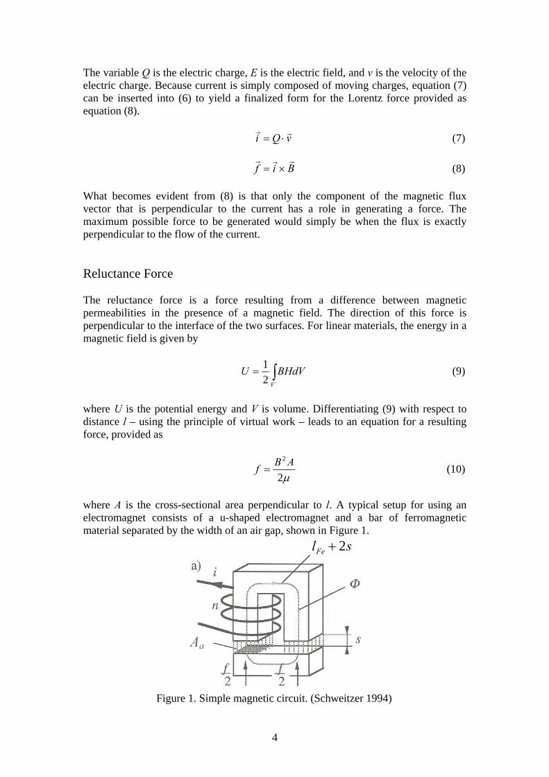
where A is the cross-sectional area perpendicular to l. A typical setup for using an electromagnet consists of a u-shaped electromagnet and a bar of ferromagnetic material separated by the width of an air gap, shown in Figure 1.

Figure 1. Simple magnetic circuit. (Schweitzer 1994)

Aa

slFe 2+

5

The variable Φ illustrates the closed-circuit path of the magnetic flux. Starting with equation (9), the energy in the air gap can be shown to be

sAHBU aaaa 221

= (11)

where s is the size of the air gap. Evaluating equation (1) for the magnetic circuit of Figure 1 yields expression (12). The magnetic flux has been solved for from (12) with the help of equations (3) and (4) and provided as equation (13). nisHHlHds aFeFe =+=∫ 2 (12)

⎟⎟⎠

⎞⎜⎜⎝

⎛+

=s

lNIB

r

Fe 20

µ

µ (13)

The variable n is the number of coils and NI together is often capitalized and called the magnetomotive force. The main assumption in evaluating (12) was that the magnetic flux does not leave the boundaries of the air gap, which does happen in actual operation of such apparatuses. To facilitate development of this analysis, the model in Figure 2 will now be used, instead of the model from Figure 1, which more accurately illustrates the situation.

Figure 2. Single electromagnet with shaft. (Schweitzer 1994) The functioning principle is the same, but the geometry reflects a real system much closer. Employing once again the principle of virtual displacement with equation (11) and simplifying with equations (3) and (13) leads to the following expression for the force exerted on a rotating shaft by an electromagnet.

αµ

µ cos2

2

0 arFe

Asl

nif ⎟⎟⎠

⎞⎜⎜⎝

⎛+

= (14)

The reason for the cosine term in (14) can be seen by examining the geometry of Figure 2. The only variables in equation (14) are the current, i, and the air gap, s.

6

After making the assumption that the permeability of the iron, µr is much greater in magnitude than the length of the magnetic circuit through the iron, lFe, the dependence of the force on the gap width and current become much clearer: the force is quadratically proportional to the current and inversely quadratically proportional to the gap width. All the other terms are constants. This relationship will be important in analyzing the controller equations. Force Linearization For any active magnetic bearing system, the main components consist of the electromagnet, rotor, sensor, controller, and amplifier. Now the electromagnet-rotor system will be further examined to see how the governing equations can be obtained for use in the controller. The force exerted by a magnet behaves much differently than that of a spring. The force of a spring increases linearly as displacement increases, whereas the force of a magnet is inversely proportional to the square of an increase in distance. As the distance between the magnet and the object subjected to its force decreases, the force levels off at a point when the material becomes saturated with the magnetic flux. For a mechatronic system, higher order relationships complicate matters and make it more difficult to implement a controller. For this reason the magnetic force must be linearized around the operating point., but to do so, the effects of current and position must be evaluated independently. With constant current and position defined as deviation from the operating point, and in the opposite direction as previously defined in order to achieve a positive correlation, a tangent line to the magnetic force curve at the operating point is drawn as seen in Figure 3.

Figure 3. Dependence of magnetic force on position. The force-displacement factor ks is used to describe the slope of the tangent line. With constant position and current defined as deviation from current at the operating point, a tangent line at the operating point is used in Figure 4 as well.

Figure 4. Dependence of magnetic force on current.

7

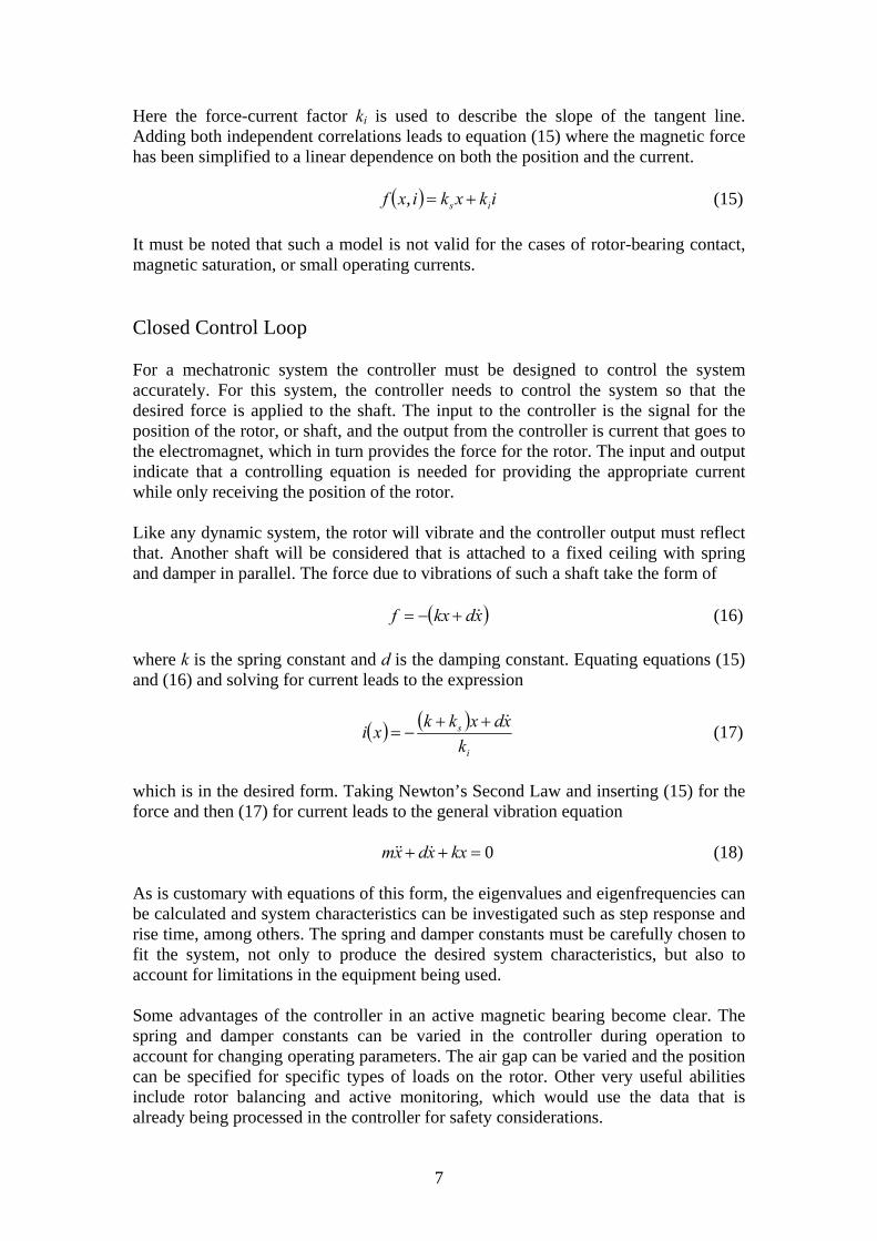
Here the force-current factor ki is used to describe the slope of the tangent line. Adding both independent correlations leads to equation (15) where the magnetic force has been simplified to a linear dependence on both the position and the current. ( ) ikxkixf is +=, (15) It must be noted that such a model is not valid for the cases of rotor-bearing contact, magnetic saturation, or small operating currents. Closed Control Loop For a mechatronic system the controller must be designed to control the system accurately. For this system, the controller needs to control the system so that the desired force is applied to the shaft. The input to the controller is the signal for the position of the rotor, or shaft, and the output from the controller is current that goes to the electromagnet, which in turn provides the force for the rotor. The input and output indicate that a controlling equation is needed for providing the appropriate current while only receiving the position of the rotor. Like any dynamic system, the rotor will vibrate and the controller output must reflect that. Another shaft will be considered that is attached to a fixed ceiling with spring and damper in parallel. The force due to vibrations of such a shaft take the form of ( )xdkxf +−= (16) where k is the spring constant and d is the damping constant. Equating equations (15) and (16) and solving for current leads to the expression

( ) ( )i

s

kxdxkkxi ++

−= (17)

which is in the desired form. Taking Newton’s Second Law and inserting (15) for the force and then (17) for current leads to the general vibration equation 0=++ kxxdxm (18) As is customary with equations of this form, the eigenvalues and eigenfrequencies can be calculated and system characteristics can be investigated such as step response and rise time, among others. The spring and damper constants must be carefully chosen to fit the system, not only to produce the desired system characteristics, but also to account for limitations in the equipment being used. Some advantages of the controller in an active magnetic bearing become clear. The spring and damper constants can be varied in the controller during operation to account for changing operating parameters. The air gap can be varied and the position can be specified for specific types of loads on the rotor. Other very useful abilities include rotor balancing and active monitoring, which would use the data that is already being processed in the controller for safety considerations.

8

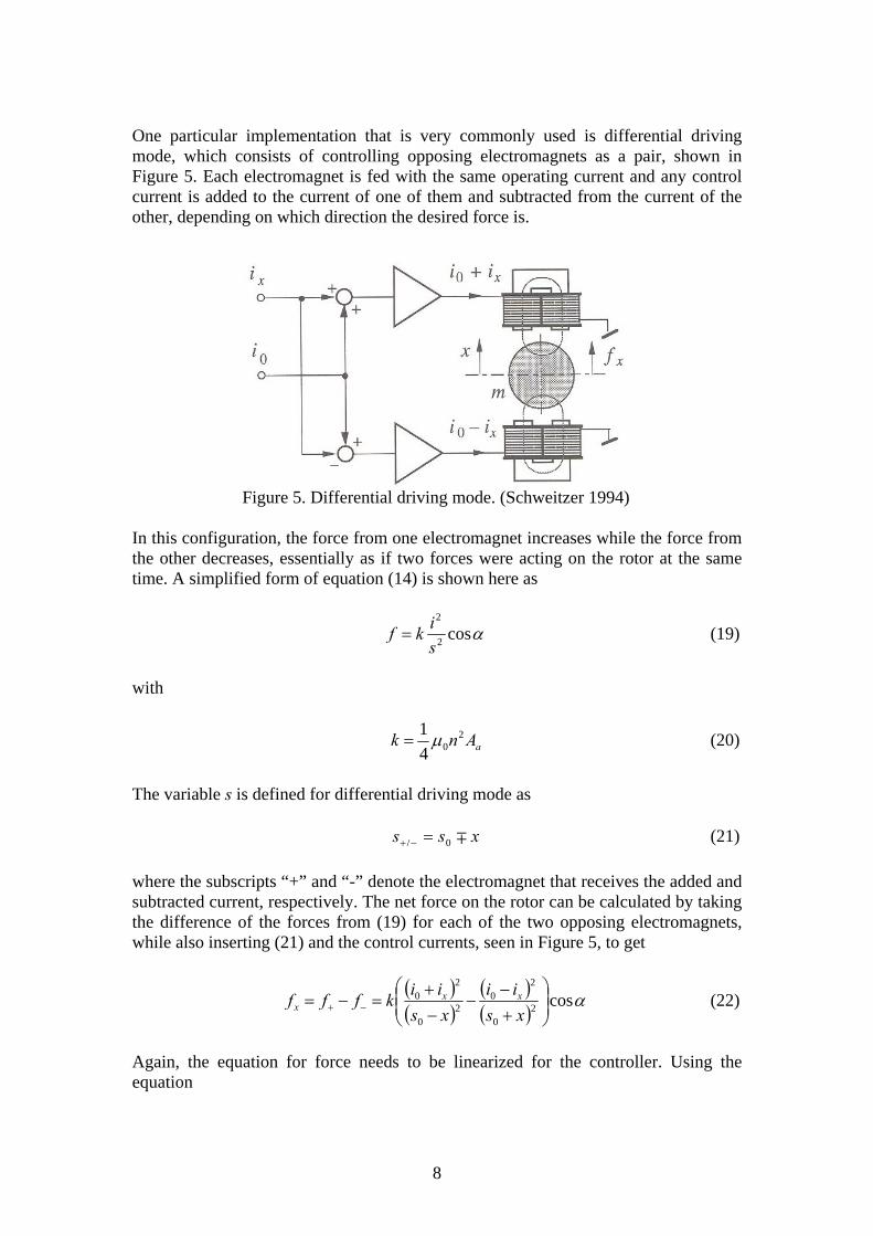
One particular implementation that is very commonly used is differential driving mode, which consists of controlling opposing electromagnets as a pair, shown in Figure 5. Each electromagnet is fed with the same operating current and any control current is added to the current of one of them and subtracted from the current of the other, depending on which direction the desired force is.

Figure 5. Differential driving mode. (Schweitzer 1994) In this configuration, the force from one electromagnet increases while the force from the other decreases, essentially as if two forces were acting on the rotor at the same time. A simplified form of equation (14) is shown here as

αcos2

2

sikf = (19)

with

aAnk 204

1 µ= (20)

The variable s is defined for differential driving mode as xss ∓0/ =−+ (21) where the subscripts “+” and “-” denote the electromagnet that receives the added and subtracted current, respectively. The net force on the rotor can be calculated by taking the difference of the forces from (19) for each of the two opposing electromagnets, while also inserting (21) and the control currents, seen in Figure 5, to get

( )( )

( )( )

αcos20

20

20

20

⎟⎟⎠

⎞⎜⎜⎝

⎛

+−

−−+

=−= −+ xsii

xsiikfff xx

x (22)

Again, the equation for force needs to be linearized for the controller. Using the equation

9

xxfi

iff

x

xx

xx

xx ⋅

∂∂

+⋅∂∂

=00

(23)

and evaluating the partial differentials yields

xskii

skif xx ⎟⎟

⎠

⎞⎜⎜⎝

⎛+⎟⎟

⎠

⎞⎜⎜⎝

⎛= αα cos4cos4

30

20

20

0 (24)

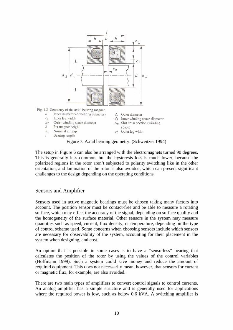
which has the same form as the original linearization of force from equation (15). Bearing Geometry Typical bearing geometry and descriptions of the components are provided for radial bearings in Figure 6 and for axial bearings in Figure 7.

Figure 6. Radial bearing geometry. (Schweitzer 1994)

10

Figure 7. Axial bearing geometry. (Schweitzer 1994) The setup in Figure 6 can also be arranged with the electromagnets turned 90 degrees. This is generally less common, but the hysteresis loss is much lower, because the polarized regions in the rotor aren’t subjected to polarity switching like in the other orientation, and lamination of the rotor is also avoided, which can present significant challenges to the design depending on the operating conditions. Sensors and Amplifier Sensors used in active magnetic bearings must be chosen taking many factors into account. The position sensor must be contact-free and be able to measure a rotating surface, which may effect the accuracy of the signal, depending on surface quality and the homogeneity of the surface material. Other sensors in the system may measure quantities such as speed, current, flux density, or temperature, depending on the type of control scheme used. Some concerns when choosing sensors include which sensors are necessary for observability of the system, accounting for their placement in the system when designing, and cost. An option that is possible in some cases is to have a “sensorless” bearing that calculates the position of the rotor by using the values of the control variables (Hoffmann 1999). Such a system could save money and reduce the amount of required equipment. This does not necessarily mean, however, that sensors for current or magnetic flux, for example, are also avoided. There are two main types of amplifiers to convert control signals to control currents. An analog amplifier has a simple structure and is generally used for applications where the required power is low, such as below 0.6 kVA. A switching amplifier is

11

used in high power applications. It introduces a high remagnetization loss, due the induced eddy currents from the switching, but is more efficient than an analog amplifier and so it has lower overall losses. Electrical Response of System Like any electrical system, there is a slight delay in signals that are carried through the wires. In the case of an active magnetic bearing, the overwhelming resistance in the circuit comes from the inductance of the electromagnets. To get an accurate picture of system performance, several factors need to be accounted for using Kirchhoff’s Law for voltage in a closed electrical circuit. The result is

xkdtdiLRiu u++= (25)

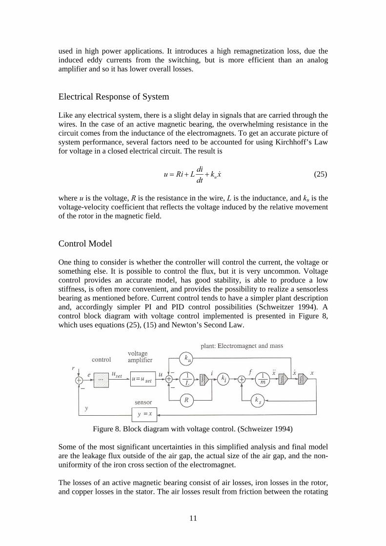
where u is the voltage, R is the resistance in the wire, L is the inductance, and ku is the voltage-velocity coefficient that reflects the voltage induced by the relative movement of the rotor in the magnetic field. Control Model One thing to consider is whether the controller will control the current, the voltage or something else. It is possible to control the flux, but it is very uncommon. Voltage control provides an accurate model, has good stability, is able to produce a low stiffness, is often more convenient, and provides the possibility to realize a sensorless bearing as mentioned before. Current control tends to have a simpler plant description and, accordingly simpler PI and PID control possibilities (Schweitzer 1994). A control block diagram with voltage control implemented is presented in Figure 8, which uses equations (25), (15) and Newton’s Second Law.

Figure 8. Block diagram with voltage control. (Schweizer 1994) Some of the most significant uncertainties in this simplified analysis and final model are the leakage flux outside of the air gap, the actual size of the air gap, and the non-uniformity of the iron cross section of the electromagnet. The losses of an active magnetic bearing consist of air losses, iron losses in the rotor, and copper losses in the stator. The air losses result from friction between the rotating

12

shaft and the surrounding environment air. The iron losses result from the eddy currents, which are minimized through laminating of the rotor, and the hysteresis. Iron losses due to hysteresis loss increase when using a switching amplifier because of the additional switching not present with an analog amplifier. The copper losses are due to the resistance in the copper wire, which happens to increase with the square of the current. More than any other factor, the copper losses tend to influence the system operation the most. All the heat dissipated in the copper windings must be taken out of the system to prevent overheating. This limits the amount of power that can be pumped into the system, which can in turn limit the performance of the magnetic bearings. Rotor Dynamics The behavior of the rotor under operating conditions is another area of analysis that must be considered. Many different effects of rotation and types of rotation can be examined. There are natural vibrations and critical speeds of the rotor which must be avoided or quickly bypassed to achieve operating speed. Other phenomena of rotation include forward and backward whirl, nutation, and precession. Rotor touch-down is something that may happen during operation, in which the rotor makes physical contact to some part of the system. This can cause damage to the equipment because of the extremely high velocities involved in such applications, but simulations of this kind of event are very difficult. One way to protect the bearing equipment is to have retainer bearings in the system so that they are contacted instead of the bearings themselves. Other times when retainer bearings are useful is during maintenance, when the system is suddenly shut off for safety reasons, or when the system is normally shut down, during which at some point the electromagnets will no longer produce the force to keep the rotor levitated in place. Stresses within the rotor are also worth considering. The radial and tangential stresses can be calculated for different radii within the rotor, solid or hollow. The largest overall stress happens to be at the inside radius of a hollow shaft, which is often used to reduce the rotational moment of inertia. Shaft materials, though, have maximum velocities at which they can travel before the stress is too large. With the maximum tensile strength of a material, a maximum velocity can be calculated. For one shaft, a maximum velocity of about 300 m/s was reached, which resulted from a shaft with a rotational velocity of around 120,000 rpm (Schweizer 1994). Permanent Magnet Bearings Magnetic bearings which utilize permanent magnets instead of electromagnets have other issues during the design. The use of passive magnetic bearings has very high potential for several reasons. They can be more economical in that the control system is avoided along with the electricity for power. Without a control system then there is also fewer components that could possibly have a problem or break down. The drawbacks are that there is no active control of the system and that there is always at least one degree of freedom that is unstable. That must be supported by a normal bearing or an active magnetic bearing.

13

Some active magnetic bearings have been replaced by systems with passive systems employing permanent magnets for the reasons stated above. Typical applications for switching over to passive bearings have been not only those with generally smaller-sized equipment and systems but also for systems in which a large air gap is desired. Current increases quadratically to make up for an increase in air gap width, so energy correspondingly increases at a high rate when the air gap gets larger. The use of a permanent magnet avoids having to use more power for a system with a large air gap. Applications There are many different areas where active magnetic bearings are used and have been successful; many more are still being developed. The complexity of the system makes implementation very difficult in some instances, but the advantages of such a system can be very enticing. Some major projects include use in turbomolecular pumps, in long-term energy storage flywheel systems, and as Maglev trains, to name just a few. The Maglev trains essentially use a linear version of the basic active magnetic bearing described in this paper to achieve very high-speed trains that are safe, reliable, and emit less noise compared to regular trains. Other applications are sure to be developed in the future as the capabilities of magnetic bearings diversify.

14

References 1. Betschon, F. Design Principles of Integrated Magnetic Bearings, Diss. ETH. Nr.

13643, ETH Zürich, 2000.

2. Boden, K. & Fremerey, J.K. Industrial Realization of the “SYSTEM KFA-JÜLICH“ Permanent Magnet Bearing Lines, Proceedings of MAG ‘92 Magnetic Bearings, Magnetic Drives and Dry Gas Seals Conference & Exhibition. Lancaster: Technomic Publishing, 1998.

3. Electricity and Magnetism. Hyperphysics. Georgia State University, Dept. of Physics and Astronomy. 1 Apr. 2006 <http://hyperphysics.phy-astr.gsu.edu/Hbase/hph.html>.

4. Fremery, J.K. Permanentmagnetische Lager. Forshungszentrum Jülich, Zentralabteilung Technologie, 2000.

5. Hoffmann, K.J. Integrierte aktive Magnetlager, Diss. TU Darmstadt. Herdecke: GCA-Verlag 1999.

6. Lösch, F. Identification and Automated Controller Design for Active Magnetic Bearing Systems, Diss. ETH. Nr. 14474, ETH Zürich, 2002.

7. Maglev Monorails of the World: Shanghai, China. The Monorail Society Website. 1 Apr. 2006 <http://www.monorails.org/tMspages/MagShang.html>.

8. Maglev Train Explained, DiscoveryChannel.ca. Bell Globemedia 2005 <http://discoverychannel.ca/interactives/japan/maglev/maglev.html>.

9. Magnetic Bearings & High Speed Motors, S2M. 1 Apr. 2006

<http://www.s2m.fr/chap3/>. 10. Moon, F.C. Superconducting Levitation: Applications to Bearings and Magnetic

Transportation. New York: John Wiley & Sons, 1994.

11. Research and Development for Superconducting Bearing Technology for Flywheel Electric Energy Storage System. New Energy and Industrial Technology Development Organization (NEDO). 1 Apr. 2006 <http://www.nedo.go.jp/ english/activities/2_sinenergy/1/p04033e.html>.

12. Schwall, R. Power Systems – Other Applications: Flywheels. Power Applications of Superconductivity in Japan and Germany. WTEC Hyper-Librarian 1997 <http://www.wtec.org/loyola/scpa/04_02.htm>.

13. Schweizer, G., Bleuler, H., & Traxler, A. Active Magnetic Bearings: Basics, Properties and Applications of Active Magnetic Bearings. Zürich: Hochschulverlag AG an der ETH, 1994.

15

14. Widbro, L. Magnetic Bearings Come of Age. Revolve Magnetic Bearings Inc. 2004. MachineDesign.com. 1 Apr. 2006 <http://www.machinedesign.com/ ASP/strArticleID/57263/strSite/MDSite/viewSelectedArticle.asp>.

15. Wikipedia contributors (2006). Hysteresis. Wikipedia, The Free Encyclopedia.

April 1, 2006 <http://en.wikipedia.org/w/ index.php?title=Hysteresis&oldid=45621877>.

16. Wikipedia contributors (2006). Magnetic field. Wikipedia, The Free

Encyclopedia. April 1, 2006 <http://en.wikipedia.org/w/ index.php?title=Magnetic_field&oldid=46010831 >.