Macroeconomic Implications of “Deep Habits” in Banking

ROGER ALIAGA-DIAZ

MARIA PIA OLIVERO

Macroeconomic Implications of “Deep Habits”

in Banking

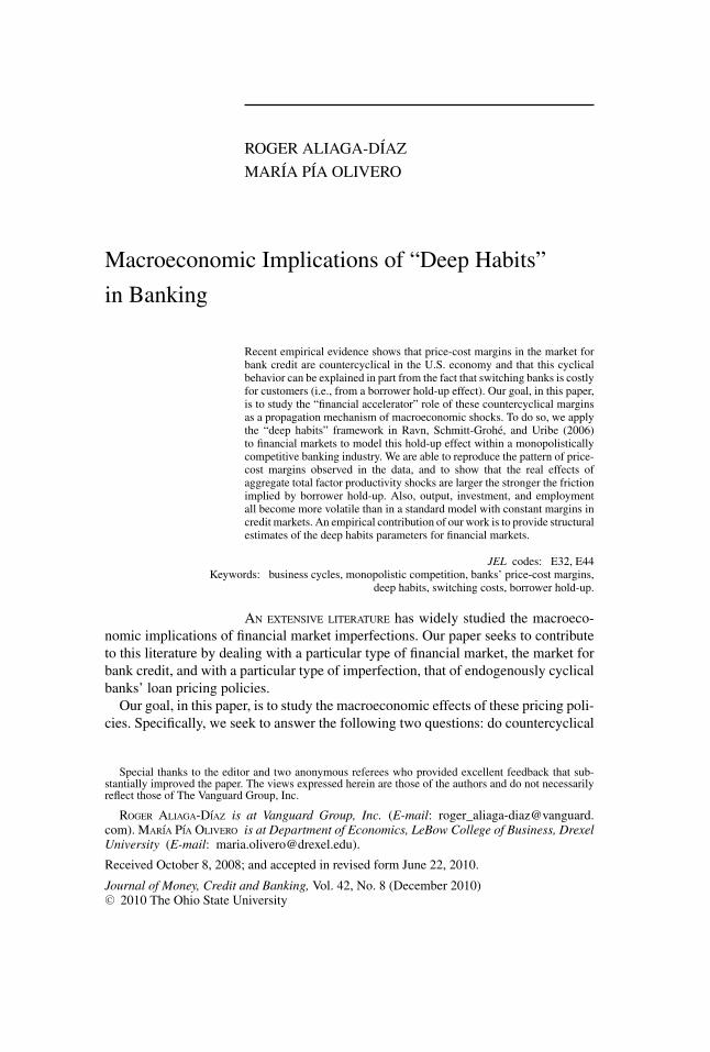
Recent empirical evidence shows that price-cost margins in the market forbank credit are countercyclical in the U.S. economy and that this cyclicalbehavior can be explained in part from the fact that switching banks is costlyfor customers (i.e., from a borrower hold-up effect). Our goal, in this paper,is to study the “financial accelerator” role of these countercyclical marginsas a propagation mechanism of macroeconomic shocks. To do so, we applythe “deep habits” framework in Ravn, Schmitt-Grohe, and Uribe (2006)to financial markets to model this hold-up effect within a monopolisticallycompetitive banking industry. We are able to reproduce the pattern of price-cost margins observed in the data, and to show that the real effects ofaggregate total factor productivity shocks are larger the stronger the frictionimplied by borrower hold-up. Also, output, investment, and employmentall become more volatile than in a standard model with constant margins incredit markets. An empirical contribution of our work is to provide structuralestimates of the deep habits parameters for financial markets.

JEL codes: E32, E44Keywords: business cycles, monopolistic competition, banks’ price-cost margins,

deep habits, switching costs, borrower hold-up.

AN EXTENSIVE LITERATURE has widely studied the macroeco-nomic implications of financial market imperfections. Our paper seeks to contributeto this literature by dealing with a particular type of financial market, the market forbank credit, and with a particular type of imperfection, that of endogenously cyclicalbanks’ loan pricing policies.

Our goal, in this paper, is to study the macroeconomic effects of these pricing poli-cies. Specifically, we seek to answer the following two questions: do countercyclical

Special thanks to the editor and two anonymous referees who provided excellent feedback that sub-stantially improved the paper. The views expressed herein are those of the authors and do not necessarilyreflect those of The Vanguard Group, Inc.

ROGER ALIAGA-DIAZ is at Vanguard Group, Inc. (E-mail: [email protected]). MARIA PIA OLIVERO is at Department of Economics, LeBow College of Business, DrexelUniversity (E-mail: [email protected]).

Received October 8, 2008; and accepted in revised form June 22, 2010.

Journal of Money, Credit and Banking, Vol. 42, No. 8 (December 2010)C© 2010 The Ohio State University

1496 : MONEY, CREDIT AND BANKING

price-cost margins in banking (defined as the spread between the interest rates onloans and deposits) act as a “financial accelerator,” working as a propagation mech-anism of aggregate total factor productivity (TFP) shocks?1 If so, do countercyclicalmargins in banking can help us better understand business cycles? Our hypothesis isthat in our setting, where recessions trigger an increase in the cost of credit, credit-dependent firms may delay their production, employment, and investment decisionsby more than in a standard model with constant price-cost margins. This, in turn,might make recessions deeper and more persistent.

The reason why in our framework recessions trigger an increase in the cost ofbank credit is associated to a borrower “hold-up” effect. The idea is that whenbanks monitor borrowers, they get an “information monopoly” over their customers’creditworthiness, which creates switching costs of changing banks for borrowers (i.e.,a borrower hold-up). In recessions, when borrowers are perceived to be in greater riskof failure, the information monopoly lets lenders hold up the borrowers for higherinterest rates, giving rise to countercyclical margins in credit markets. Several studiesin the banking literature along with our own findings presented below in Section 1support this story (see Diamond 1984, Sharpe 1990, Rajan 1992, von Thadden 1995,Dell’Ariccia 2001, Santos and Winton 2008).

We model this relationship between banks’ cyclical pricing policies and borrowerswitching costs through an application of the “deep habits” framework in Ravn,Schmitt-Grohe, and Uribe (2006) (hereafter RSGU) to financial markets. By doingso we follow their suggestion that their model can be viewed as a natural vehiclefor incorporating switching costs into dynamic general equilibrium frameworks.2

Although RSGU is not a model of informational asymmetries, their deep habitsframework is a useful and tractable way to replicate the borrower hold-up effect gen-erated by these asymmetries within a dynamic stochastic general equilibrium (DSGE)setting. The bank pricing policies in a model where borrowers exhibit deep habits inthe choice of lenders are equivalent to those that would arise in an asymmetric infor-mation model where incumbent banks accumulate proprietary information on theircustomers creditworthiness, which allows them to build an information monopolyand gives them market power. With deep habits, it is costly for borrowers to switchto a different bank and thus banks can hold up borrowers for higher interest rates justas in an asymmetric information model.

An additional value added of our work is to provide structural estimates of thedeep habits parameters for financial markets.

There are two ways in which a setup with deep habits in banking allows usto better understand business cycles. First, our model can reproduce the empiricalobservation that margins in the market for credit are more volatile than GDP in the

1. For studies documenting the countercyclical nature of these margins, see Dueker and Thornton(1997), Mandelman (2006), Aliaga-Dıaz and Olivero (2010, Forthcoming), and Olivero (2010).

2. RSGU demonstrate the formal similarity between the deep habit model and switching costs models.Nakamura and Steinsson (2006) interpret this good specific habit model as providing a specification forthe effects of switching costs.

ROGER ALIAGA-DIAZ AND MARIA PIA OLIVERO : 1497

U.S. economy. Second, our model is able to reproduce the countercyclicality of banks’price-cost margins observed in the data. Moreover, these margins are endogenouslycountercyclical in a way consistent with the presence of switching costs or borrowershold-up (see empirical evidence provided in Section 1). The intuition for this resultis as follows. Because of the hold-up effect, when choosing the interest rate on loans,banks face a trade-off between current profits and future market share: loweringinterest rates lowers current profits but allows them to build a larger future marketshare. After a positive TFP shock hits the economy, the present value of future profitsis expected to be high, which raises the lenders’ incentives to lure customers that willbe held up in the future. The future market share motive gains importance relative tothe current profits motive, and induces banks to charge lower margins.

From the simulation analysis, we conclude that aggregate TFP shocks have largerreal effects when price-cost margins are countercyclical and that these effects arelarger the stronger hold-up. Also, output, investment, and employment all becomemore volatile than in a standard model with constant margins in credit markets.Therefore, countercyclical margins act as a financial accelerator of business cycles.The supply-side effects coming from banks’ loan pricing policies in the model workto amplify the standard demand-side effects of aggregate TFP shocks.

Our results have relevant policy implications since countercyclical margins seemto provide additional grounds for stabilization policy in economies where marginsare more cyclical and where the share of bank credit in total external financing ishigher.

Related to our work are Bernanke and Gertler (1989) and Bernanke, Gertler, andGilchrist (1998, 1999). They study the role of endogenously countercyclical externalfinance premia as an amplifier of business fluctuations. Our borrower hold-up, or bor-rower switching costs, story provides an alternative way to generate countercyclicalexternal finance premia and the implied financial accelerator.

The rest of the paper is organized as follows. Section 1 presents some empiricalevidence on the cyclicality of price-cost margins in banking. Section 2 develops themodel. Section 3 presents the simulation results. Section 4 concludes and providessome directions for further research. The Appendix presents the results of a sensitivityanalysis on the calibration of the deep habits parameters.

1. THE EMPIRICAL EVIDENCE

To provide some insight on banks cyclical pricing policies, in this section, wepresent empirical evidence on the cyclical behavior of price-cost margins in banking(defined as the spread between the interest rates on loans and deposits). Margins area useful measure of the cost of external finance for borrowers since they representthe premium of the interest rate paid on loans over borrowers’ opportunity cost ofinternal funds (as measured by the interest rate on deposits).


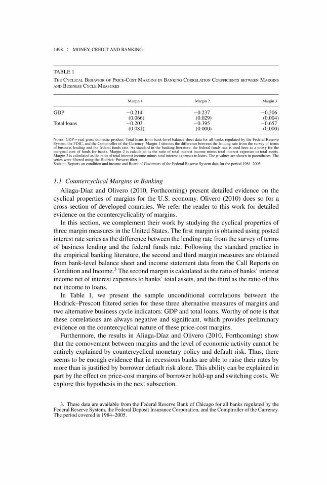
TABLE 1

THE CYCLICAL BEHAVIOR OF PRICE-COST MARGINS IN BANKING CORRELATION COEFFICIENTS BETWEEN MARGINS

AND BUSINESS CYCLE MEASURES

Margin 1 Margin 2 Margin 3

GDP −0.214 −0.237 −0.306(0.066) (0.029) (0.004)

Total loans −0.203 −0.395 −0.657(0.081) (0.000) (0.000)

NOTES: GDP = real gross domestic product. Total loans from bank-level balance sheet data for all banks regulated by the Federal ReserveSystem, the FDIC, and the Comptroller of the Currency. Margin 1 denotes the difference between the lending rate from the survey of termsof business lending and the federal funds rate. As standard in the banking literature, the federal funds rate is used here as a proxy for themarginal cost of funds for banks. Margin 2 is calculated as the ratio of total interest income minus total interest expenses to total assets.Margin 3 is calculated as the ratio of total interest income minus total interest expenses to loans. The p-values are shown in parentheses. Theseries were filtered using the Hodrick–Prescott filter.SOURCE: Reports on condition and income and Board of Governors of the Federal Reserve System data for the period 1984–2005.

1.1 Countercyclical Margins in Banking

Aliaga-Dıaz and Olivero (2010, Forthcoming) present detailed evidence on thecyclical properties of margins for the U.S. economy. Olivero (2010) does so for across-section of developed countries. We refer the reader to this work for detailedevidence on the countercyclicality of margins.

In this section, we complement their work by studying the cyclical properties ofthree margin measures in the United States. The first margin is obtained using postedinterest rate series as the difference between the lending rate from the survey of termsof business lending and the federal funds rate. Following the standard practice inthe empirical banking literature, the second and third margin measures are obtainedfrom bank-level balance sheet and income statement data from the Call Reports onCondition and Income.3 The second margin is calculated as the ratio of banks’ interestincome net of interest expenses to banks’ total assets, and the third as the ratio of thisnet income to loans.

In Table 1, we present the sample unconditional correlations between theHodrick–Prescott filtered series for these three alternative measures of margins andtwo alternative business cycle indicators: GDP and total loans. Worthy of note is thatthese correlations are always negative and significant, which provides preliminaryevidence on the countercyclical nature of these price-cost margins.

Furthermore, the results in Aliaga-Dıaz and Olivero (2010, Forthcoming) showthat the comovement between margins and the level of economic activity cannot beentirely explained by countercyclical monetary policy and default risk. Thus, thereseems to be enough evidence that in recessions banks are able to raise their rates bymore than is justified by borrower default risk alone. This ability can be explained inpart by the effect on price-cost margins of borrower hold-up and switching costs. Weexplore this hypothesis in the next subsection.

3. These data are available from the Federal Reserve Bank of Chicago for all banks regulated by theFederal Reserve System, the Federal Deposit Insurance Corporation, and the Comptroller of the Currency.The period covered is 1984–2005.


1.2 How Borrower Hold-Up and Switching Costs Give Rise to the ObservedCountercyclicality

Santos and Winton (2008) present evidence that borrower switching costs giverise to a lasting borrower–lender relationship, which allows incumbent banks toaccumulate information over time, and to eventually earn an informational monopolyover their customers. This creates a hold-up, or “lock-in,” effect that makes it costlyfor firms to switch lenders. Santos and Winton (2008) use microloan data and find thatbank-dependent firms without accessibility to public debt markets pay significantlyhigher loan rates than those firms with the accessibility, implying that banks do takeadvantage of their information monopoly. They also show that banks seem to be ableto exploit this advantage further during recessions, when borrowers are in greaterrisk of failure. They do so by providing evidence that in recessions, banks raise theirrates more for bank-dependent borrowers than for those with access to public bondmarkets, and that much of this is due to informational hold-up effects.4

To further study how this hold-up can give rise to the observed cyclicality ofmargins, in this section, we measure the empirical relationship between borrowersswitching costs and the degree of countercyclicality of margins using unbalancedpanel data for 56 countries including developing and developed economies in Northand South America, Europe, and Asia. To do so, we conduct a two-step estimationmethodology. In the first step, we use time-series techniques to obtain a measure ofthe cyclicality of credit margins in each country. In the second step, we perform across-sectional analysis, and we regress the measure of cyclicality of margins fromthe first step on a measure of switching costs and other controls.

For the first step, we use data on lending and deposit rates and real GDP fromthe IMF International Financial Statistics (IFS) for this cross-section of countries.We then calculate price-cost margins as the difference between lending and depositrates. We obtain a measure of cyclicality of margins as the unconditional correlationcoefficient between Hodrick–Prescott filtered margins and GDP.

In the second step, we regress this cyclicality on a measure of switching costsin banking. Switching costs measures are from Yuan (2009) and Olivero and Yuan(2009), who obtain switching costs for a cross-section of countries by structurallyestimating the model in Kim, Kliger, and Vale (2003). Yuan uses bank-level balancesheet and income statement data from Bankscope to estimate switching costs for 25 ofthe countries in our sample. Olivero and Yuan obtain them for the United States usingdata from the Call Reports on Condition and Income. For the remaining countriesin our sample, we obtain the switching costs estimates as the predicted values froma regression of the switching cost measures in Yuan and in Olivero and Yuan onmargins.

In the second step regression of the cyclicality of margins on these switching costs,we also control for relative country size (measured as the ratio of each country’s GDPto GDP in the United States), the degree of openness in each country (proxied by the

4. Hale and Santos (2009) show that firms are able to borrow from banks at lower interest rates afterthey issue for the first time in the public bond market. They interpret this finding as evidence that banksdo indeed price their informational monopoly.


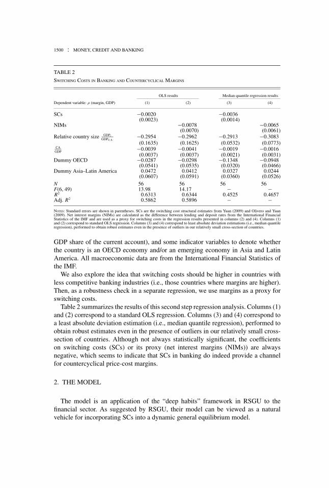
TABLE 2

SWITCHING COSTS IN BANKING AND COUNTERCYCLICAL MARGINS

OLS results Median quantile regression results

Dependent variable: ρ (margin, GDP) (1) (2) (3) (4)

SCs −0.0020 −0.0036(0.0023) (0.0014)

NIMs −0.0078 −0.0065(0.0070) (0.0061)

Relative country size GDPiGDPU.S.

−0.2954 −0.2962 −0.2913 −0.3083(0.1635) (0.1625) (0.0532) (0.0773)

CAGDP

−0.0039 −0.0041 −0.0019 −0.0016(0.0037) (0.0037) (0.0021) (0.0031)

Dummy OECD −0.0287 −0.0298 −0.1348 −0.0948(0.0541) (0.0535) (0.0320) (0.0466)

Dummy Asia–Latin America 0.0472 0.0412 0.0327 0.0244(0.0607) (0.0591) (0.0360) (0.0526)

N 56 56 56 56F(6, 49) 13.98 14.17 − −R2 0.6313 0.6344 0.4525 0.4657Adj. R2 0.5862 0.5896 − −NOTES: Standard errors are shown in parentheses. SCs are the switching cost structural estimates from Yuan (2009) and Olivero and Yuan(2009). Net interest margins (NIMs) are calculated as the difference between lending and deposit rates from the International FinancialStatistics of the IMF and are used as a proxy for switching costs in the regression results presented in columns (2) and (4). Columns (1)and (2) correspond to standard OLS regression. Columns (3) and (4) correspond to least absolute deviation estimations (i.e., median quantileregression), performed to obtain robust estimates even in the presence of outliers in our relatively small cross-section of countries.

GDP share of the current account), and some indicator variables to denote whetherthe country is an OECD economy and/or an emerging economy in Asia and LatinAmerica. All macroeconomic data are from the International Financial Statistics ofthe IMF.

We also explore the idea that switching costs should be higher in countries withless competitive banking industries (i.e., those countries where margins are higher).Then, as a robustness check in a separate regression, we use margins as a proxy forswitching costs.

Table 2 summarizes the results of this second step regression analysis. Columns (1)and (2) correspond to a standard OLS regression. Columns (3) and (4) correspond toa least absolute deviation estimation (i.e., median quantile regression), performed toobtain robust estimates even in the presence of outliers in our relatively small cross-section of countries. Although not always statistically significant, the coefficientson switching costs (SCs) or its proxy (net interest margins (NIMs)) are alwaysnegative, which seems to indicate that SCs in banking do indeed provide a channelfor countercyclical price-cost margins.

2. THE MODEL

The model is an application of the “deep habits” framework in RSGU to thefinancial sector. As suggested by RSGU, their model can be viewed as a naturalvehicle for incorporating SCs into a dynamic general equilibrium model.


In a context of asymmetric information on borrowers creditworthiness, banksgradually accumulate this information over time as they lend repeatedly to theircustomers, eventually earning an informational monopoly over these borrowers. Thiscreates a borrower hold-up effect, which makes it costly for borrowers to switchlenders and to have to start signaling this information to a new bank. Thus, borrowerhold-up gives rise to SCs. In recessions when these informational asymmetries aremore pronounced and when borrowers are in greater risk of failure, incumbent bankscan further exploit their advantage and raise lending rates by more than in a standardmodel that lacks this friction.

Although RSGU is not a model of informational asymmetries, their deep habitsframework is still a useful and tractable way to replicate the borrower hold-up effectin a DSGE setting. With deep habits, it is costly for borrowers to switch to a differentbank, and thus banks can hold up borrowers for higher interest rates, just as in afully microfounded informational monopoly model. Admittedly, this is a reducedform of incorporating the effects of informational asymmetries into a DSGE model.However, a formal setup of asymmetric information in a DSGE framework wouldrequire heterogeneous agent solution methods, something that is beyond the scope ofthis paper.5

This is a closed economy with a household sector, a production sector and financialintermediaries (hereafter called banks). Households take consumption–saving andlabor–leisure decisions to maximize their expected lifetime utility. Firms producegoods using labor and capital. To finance investment spending, firms use a compositeof heterogeneous bank loans. Banks use household savings to provide loans in amonopolistically competitive market.

We now proceed to present the optimization problems of all agents in this economy.

2.1 Firms

There is a continuum of measure one of firms indexed by j ∈ [0, 1]. In each periodt firm j sells output (Y j

t ) in a competitive goods market, produced using labor (h jt )

and capital (K jt ). To finance investment spending, firm j uses a composite (x j

t ) ofimperfectly substitutable heterogeneous loans provided by a continuum of mass oneof banks. Each bank is indexed by i , and firm j borrows from a subset ψ j of them.6

In this setup, firms engage in multiple banking relationships by borrowing fromseveral banks in the economy. This is in line with the rich empirical evidence

5. Aliaga-Dıaz and Olivero (2008) provide such a model.6. There is abundant evidence on the existence of product differentiation in banking that makes the

financial services from different banks imperfectly substitutable from the point of view of borrowers.Banks can differentiate their loans by targeting the financial services that they provide together with aloan (i.e., firm monitoring, valuation of collateral, and investment project evaluation) toward particularsectors of economic activity. Also, banks can choose various quality characteristics to build reputation anddifferentiate from competitors, like equity ratios, size, loss avoidance, etc. (Kim, Kristiansen, and Vale2005). Last, lenders use different product packages and the extensiveness and location of their branches(Northcott 2004), personalized service, accessibility to the institution’s executives, hours of operation andATM, and remote access availability (Cohen and Mazzeo 2004) to differentiate their services from thoseof competitors.


presented by Ongena and Smith (2000a) and references therein.7 Fama (1985), Sharpe(1990), Rajan (1992), Petersen and Rajan (1994), Hart (1995), von Thadden (1995),Bolton and Scharfstein (1996), Detragiache, Garella, and Guiso (1999), Neubergerand Schacht (2005), and Vulpes (2005) also study various reasons for firms to borrowfrom multiple banks.

To model the existence of borrower hold-up effects and costs of switching banks,the loan composite x j

t is assumed to depend on past levels of borrowing, as definedby equations (1) and (2),

x jt =

[∫ ψ j

0

(l ji t − θsit−1

)1− 1η di

]1/(1− 1η

)

, (1)

sit−1 = ρssit−2 + (1 − ρs)li t−1, (2)

where l ji t is firm j’s demand for credit from bank i in period t , and η > 1 is the elasticity

of substitution across varieties. This specification for the Dixit–Stiglitz aggregatorimplies that each firm j borrows from a subset ψ j of all banks in the economy.

The second term in x jt is intended to capture the borrower hold-up effect. sit−1

measures the stock of firm–bank relationships and the parameter θ measures thedegree of hold-up.

The fact that θ > 0 implies that the current demand for credit is a function of pastborrowing levels. It will become clear later that θ > 0 also implies that the interestrate elasticity of the demand for loans and, hence price-cost margins in the marketfor credit are cyclical, and that they exhibit a behavior consistent with the empiricalevidence presented in Section 1. When θ = 0 the model boils down to the benchmarkversion with constant interest rate elasticity of the demand for credit, pinned downby the elasticity of substitution across varieties η.

Equation (2) defines the stock s as a function of the cross-sectional average levelof borrowing from bank i in period t − 1. This average satisfies li t−1 ≡ ∫ μi

0 l ji t−1d j ,

where μi is the subset of j firms that borrow from bank i . This average is takenas exogenous by each individual atomistic firm. The fact that the stock sit−1 is afunction of the average level of borrowing implies that habits are external to theborrower.8 This can be rationalized through banks exhibiting economies of scale in

7. According to various studies cited by Ongena and Smith (2000a), the average number of bankrelationships is 15.2 in Italy; 11 in Portugal, France, and Belgium; 9.7 in Spain; 8.1 in Germany; 7.4 inGreece; 5 in Austria, Luxembourg, and the Czech Republic; 4 in Hungary; 3 in Japan, Finland, Switzerland,Denmark, the Netherlands, Poland, Ireland, and the United Kingdom; and 2 in Sweden, Norway, and theUnited States.

8. As in RSGU, this assumption makes the model analytically tractable, since it preserves the separationof the dynamic problem of choosing total borrowing over time from the static problem of choosingindividual borrowing from each bank at any given point in time. If this was not the case, the currentdemand from each bank i would depend both on its current relative interest rate and on all future expectedrates. Therefore, each bank would face an incentive to renege from past interest rate promises, and theproblem would no longer be time consistent.


the management of informational asymmetries. Thus, the more firms bank with onebank, the larger the information monopoly for that bank.

Equation (2) gives the law of motion for the stock s, where the parameter ρs ∈[0, 1) measures the persistence or duration of the hold-up effects or, in other words,the speed of adjustment of these effects to variations in the previous period cross-sectional average lit−1. The fact that ρs > 0 makes the model general enough to allowfor these effects to last over several periods. When ρs = 0, hold-up effects are veryshort-lived and last for only one period.

In each period t , firm j chooses investment (I jt ), employment (h j

t ), the loanscomposite (x j

t ) and borrowing from each bank i (l ji t ) to maximize the expected

present discounted value of its lifetime profits. Its optimization problem is given by9

maxK j

t+1,I jt ,h j

t ,xjt ,l j

i t

E0

∞∑t=0

t∏m=0

qmπj

t qm = βm UCm

UCm−1

s.t.

eq.(1),

eq.(2),

πj

t = At F(K j

t , h jt

) − wt hjt − I j

t + x jt −

∫ ψ j

0(1 + Rit−1)l j

i t−1di + �jt , (3)

K jt+1 = I j

t + (1 − δ)K jt , (4)

∫ ψ j

0l ji t di ≥ φ I j

t φ ≤ 1, (5)

ln(At+1) = ρln(At ) + εt , (6)

where ψ j is the subset of i banks that firm j borrows from, and where as in RSGU�

jt ≡ θ

∫ ψ j

0(1+Rit )(1+Rt )

sit−1di . Equation (3) corresponds to firm j’s cash flow, where wt

is the wage rate and Rit−1 is the interest rate contracted with bank i in period t − 1,on loans to be repaid in period t . This equation defines firm j’s profits in period tas sales revenues plus what the firm obtains from borrowing minus the sum of labor,investment, and borrowing costs.

Equation (3) is a key equation in the model, since it helps to understand howdeep habits work to provide microfoundations for SC models. In that sense, what the

9. Firms in this economy are owned by households, and therefore, their discount factor q is given bythe households’ intertemporal marginal rate of substitution.


firms/borrowers actually borrow is l jt ≡ ∫ ψ j

0 l ji t di and they repay

∫ ψ j

0 (1 + Rit )lji t di

one period later. However, what they effectively borrow is given by the term(x j

t + �jt ) = [

∫ ψ j

0 (l jit − θsit−1)1−1/η di]

11−1/η + θ

∫ ψ j

0(1+Rit)(1+Rt )

sit−1 di in the profit func-tion. Thus, the wedge between these two can be thought of as the cost of switchingbetween bank i and any other rival bank. This cost is a function of the differencebetween the rate charged by bank i (Ri) and the market rate (R). To see this analyti-cally, consider the case for which η → ∞. In this case, effective borrowing amountsto:

∫ ψ j

0 l ji t di − θ

∫ ψ j

0 sit−1(Rt −Rit )(1+Rt )

di , while actual borrowing amounts to:∫ ψ j

0 l ji t di .

Therefore, the wedge between the two or SCs is represented by: θ∫ ψ j

0 sit−1(Rt −Rit )(1+Rt )

di .Notice that, as discussed in RSGU, this is still a model where there is no discrete

switching when a seller raises its price, but rather a gradual loss of customers forthat seller. This is important because it makes the general equilibrium model com-putationally tractable and suitable to explore the macroeconomic and business cycleimplications of deep habits in banking. However, even without discrete switching,there is still a wedge between what firms actually borrow (i.e., the amount that theyrepay in t + 1) and what they effectively borrow. This wedge is what we refer to asSCs in this model.

Equation (4) gives the standard law of motion for the firm’s capital stock.Equation (5) introduces the need for bank financing into the model, and it states

that each firm needs to finance at least a fraction φ of its investment spending withexternal borrowing.10

Last, equation (6) describes the exogenous process followed by TFP, where εt

follows an i.i.d. distribution with mean zero and standard deviation σ ε .From this problem, firm j’s optimal demand for credit from bank i is

l ji t =

(1 + Rit

1 + Rt

)−η

x jt + θsit−1, (7)

where (1 + Rt ) ≡ [∫ ψ j

0 (1 + Rit )1−η di]1

1−η is the nominal price index for the loancomposite.

10. With market power in banking and (1 + Ri) ≥ q−1 firms will always prefer to finance investmentwith internal rather than with external resources, and borrowing would be zero if this condition was notimposed. In other words, φ would always equal 0 if it was optimally chosen by borrowers. Therefore,equation (5) always binds in equilibrium. Equation (5) is actually the opposite of a standard borrowingconstraint that sets an upper limit on borrowing equal to a fraction of the borrower’s collateral. Onthe contrary, this financing constraint sets a lower limit on external borrowing, and it is needed forbanks and external credit to play a role in the model. Admittedly, it is an ad hoc way to incorporatemeaningful financial intermediation into the model. Modeling the existence of financial intermediariesfrom first principles through their role in liquidity provision, monitoring of borrowers credit worthinessor management of maturity mismatches has been widely studied in the past, and it is beyond the scope ofour paper. The parameter φ is calibrated to match the ratio of external credit to business investment in thedata.


2.2 The Banking Sector

There is a continuum of mass one of banks indexed by i ∈ [0, 1]. Each varietyof loans/financial services is produced by a bank operating in a monopolisticallycompetitive loan market. Banks are competitive in the market for deposits.

In each period t bank i chooses its demand for deposits (Dit) and the interestrate charged on loans (Rit) to maximize the expected present discounted value of itslifetime profits. Bank i’s optimization problem is given by11

maxDit,Rit

E0

∞∑t=0

t∏m=0

qm it qm = βm UCm

UCm−1

s.t.

it = Dit − Lit + (1 + Rit−1)Lit−1 − (1 + rt−1)Dit−1 − κ, (8)

Lit = Dit, (9)

Lit ≡∫ μi

0l jit dj =

∫ μi

0

[(1 + Rit

1 + Rt

)−η

x jt + θsit−1

]dj, (10)

where μi is the subset of j firms that borrow from bank i .Equation (8) is the bank’s cash flow in period t , where r t−1 is the common risk-free

interest rate on deposits paid by all banks. κ denotes the fixed costs of productionintroduced to guarantee no entry in the monopolistically competitive banking sector.The presence of κ ensures that profits are relatively small on average, in spite ofequilibrium price-cost margins being significantly positive. Equation (9) is bank i’sbalance sheet condition, and equation (10) shows the aggregate demand from a μi

subset of j firms that bank i internalizes.The Lagrangian of bank i’s problem is given by

� = E0

∞∑t=0

Q0,t

{(Rit−1 − rt−1)Lit−1 − κ

+ νit

[− Lit +

∫ μi

0

[(1 + Rit

1 + Rt

)−η

x jt + θsit−1

]dj

]},

Q0,t = β t UCt

UC0

,

where the multiplier ν it measures the shadow value of lending an extra dollar by banki in period t .

11. Banks are owned by households so that their discount factor q is given by the households’intertemporal marginal rate of substitution.


The first-order conditions with respect to Lit and Rit are, respectively,

νit = (Rit − rt )Et Qt,t+1 + θ Et Qt,t+1νit+1(1 − ρs), (11)

Lit Et Qt,t+1 = −νit∂Lit

∂ Rit. (12)

Equation (11) states that the value of lending an extra dollar in period t is composedof two terms: the short-run returns of that operation ((Rit − rt)Et Qt,t+1), and the futureexpected profits associated with the fact that a share of this lending will be held upin period t + 1. Equation (12) states that the marginal revenue of an increase in theinterest rate (given by the discounted value of the loans Lit Et Qt,t+1) has to equalthe marginal cost of that increase (given by the resulting reduction in the quantitydemanded of loans ∂Lit

∂ Ritevaluated at the shadow price ν it).

We are now able to use equations (11) and (12) to formally show the equivalencebetween this deep habits model and a SC model a la Klemperer (1995). Let V (Lit−1)be the value of the maximized objective function for the bank for any given Lit−1.Then, we can represent the bank’s optimization problem as

V (Lit−1) = maxRit,Lit

{(Rit−1 − rt−1)Lit−1 − κ + Et Qt,t+1V (Lit)

}s.t.

Lit ≡∫ μi

0l jit dj =

∫ μi

0

[(1 + Rit

1 + Rt

)−η

x jt + θsit−1

]dj.

Using the constraint to eliminate Lit, the FOC with respect to Rit is

∂ it

∂ Rit+ Et Qt,t+1

∂V (Lit)

∂Lit

∂Lit

∂ Rit= 0.

This equation is analogous to equation (2′) in Klemperer (1995), where firm F’sFOC is

∂π Ft

∂pFt

+ δ∂V F

t+1

∂σ Ft

∂σ Ft

∂pFt

= 0,

where π Ft , pF

t , and σ Ft denote firm F’s profits, price and market share in period t ,

respectively. As in RSGU, the equivalence with the Klemperer (1995) model becomesobvious noting that pF

t and σ Ft are linearly related to Rit and Lit, respectively.

Still an important difference between the two models is the absence of discreteswitching in equilibrium in the deep habits model, where each firm j can distribute itsborrowing identically among a subset ψ j of banks, and still each bank i faces a gradualloss of market share if it raises its interest rate Ri above R. This is a useful feature that


facilitates numerical tractability of the DSGE model when studying macroeconomicissues.

2.3 Households

A representative household takes consumption (Ct), savings and labor supplydecisions in this economy. Each household derives disutility from working and isallowed to save by accessing a competitive market for bank deposits (Dt) in eachperiod t ≥ 0. Firms’ and banks’ profits are rebated to households in a lump-sumfashion.

The optimization problem for the representative household is given by

maxCt ,ht ,Dit

E0

∞∑t=0

β tU (Ct , ht )

s.t.

Ct +∫ 1

0Dit di = wt ht + (1 + rt−1)

∫ 1

0Dit−1 di +

∫ 1

0π

jt dj +

∫ 1

0 it di, (13)

and a no-Ponzi game constraint, taking as given initial deposit holdings and theprocesses for wt , π

jt , and it.

2.4 Deep Habits and Price-Cost Margins in Banking

In this section, we obtain an equation for equilibrium price-cost margins in themarket for bank credit, and we discuss the role that deep habits play in shaping thecyclical nature of these margins.

Working with equations (11) and (12) and using the approximation 1+Rit1+Rt

≈e(Rit −Rt ) ≈ (1 + Rit − Rt ), we can derive an expression for the price-cost margin(Rit − rt) charged by each noncompetitive bank i in this economy as12

(Rit − rt ) ={η (ψ)

1(1−η)

[1 − θρs

sit−2

li t− θ (1 − ρs)

γt

]}−1

− θ (1 − ρs)Et Qt,t+1νi t+1

Et Qt,t+1, (14)

where γt ≡ li tli t−1

denotes the growth rate of loans at time t .

The expression {η(ψ)1

(1−η) [1 − θρssit−2

li t− θ(1−ρs )

γt]} gives the short-run interest rate

elasticity of the demand for credit faced by bank i . It is easily seen that the marginbetween Rit and rt is inversely related to this elasticity. An increase in the level

12. The approximation error tends to cancel out since the same transformation is performed on thenumerator and the denominator of the original expression. The details on this derivation are presented ina mathematical appendix available at https://faculty.lebow.drexel.edu/OliveroM/.


of economic activity (reflected in an increase in lt and γ t) raises the elasticity andlowers the margin. The intuition is the following: as a result of the hold-up effect,when choosing the interest rate on loans banks face a trade-off between current profitsand future market share: lowering interest rates lowers current profits but allows themto build larger future market shares. With autocorrelated TFP shocks, an increase inthe current demand for credit implies that the present value of future profits is high,which raises lenders’ incentives to lure customers that will be held up in the future.The future market share motive dominates over the current profits motive. Thus,banks start charging lower margins to lure customers and to increase their currentmarket share. A higher market share today implies more customers for the future.Therefore, the optimal price-cost margin for each bank is diminishing in the level ofcurrent demand.

The spread also depends negatively on the value of future perunit profits discountedto period t + 1 (as measured by ν t+1).13 The intuition here is that an increase in futureexpected profits raises the value of a higher future market share. Thus, banks have anincentive to lower margins today to gain a higher customer base in the future, even ifthis implies giving up current profits.

Last, notice that if θ = 0, then (Rit − rt ) = 1η(ψ j )−

1(1−η) , and the model collapses

to the benchmark version with no borrower hold-up and constant price-cost marginspinned down by the inverse of the elasticity of substitution across varieties.

It is important to highlight that we obtain this hold-up effect in equilibrium even ina model where agents are forward looking. These agents do anticipate that they mightbe being currently lured with lower interest rates and that this might be happeningat the expense of higher future rates. However, even in this case, these forward-looking agents cannot avoid higher rates because hold-up is modeled as external inthis framework. In other words, habits are modeled at the cross-sectional sector levelinstead of at the individual borrower’s level, and borrowers have no control over theexternal component of habits.

This intuition is also evident from the model’s FOCs. In our framework of externalhabits, the demand for loans in equation (7) is only a function of current relative pricesand the stock of habits. Conversely, the current demand for a particular variety dependsalso on all future expected relative prices when habits are internal.14 Therefore, ina model with forward-looking agents and internal habits, that is, in a model wheredemand is a function of both current and future prices, banks may be less able tocharge lower interest rates today to lure borrowers at the expense of higher futurerates.15

13. It can be shown that ν t is the present discounted value of expected future perunit profits inducedby a unit increase in current lending.

14. See Section 4.3 of RSGU for the internal habits extension of their model.15. Notice that in the internal habits model, the problem is no longer time consistent; since then,

monopolists have the incentive to renege from price promises made in the past. Thus, this statement isconditional on banks not reneging from their past promises. Special thanks to one of the referees forpointing out the need for this analysis and how it relates to the external habits formulation of the model.


TABLE 3

BENCHMARK CALIBRATION

Preference parameters

β = 0.99 σ = 2ω = 0.2

Financing parametersθ = 0.72 η = 190 φ = 0.42ρs= 0.85Production parametersα = 0.64 δ = 0.018TFP processσ ε = 0.007 ρ = 0.95

3. MODEL SOLUTION

3.1 Calibration

The model is calibrated at a quarterly frequency to the U.S. economy followingthe standards in the RBC literature.

Preferences are assumed to be isoelastic and of the constant relative risk aversiontype. The utility function is U (C, h) = (Cω(1−h)1−ω)1−σ

(1−σ ) , where σ > 1 is the inverse ofthe intertemporal elasticity of substitution. The parameter σ is set to 2, and ω to 0.2.

The production function is of the Cobb–Douglas type F(K , h) = AK 1−αhα and itis assumed to exhibit constant returns to scale. The labor share in GDP α is set to 0.64.The depreciation rate δ is set to 0.018 to match the 0.076 investment to capital ratiofor annual data in Cooley and Prescott (1995). φ is set to 0.42 to match the mean ratioof credit market instruments to nonresidential gross fixed investment for nonfinancialbusinesses in the U.S. Flows of Funds Accounts data for the period 1946–2008.16

The discount factor β is set to match the average quarterly 10-year interest rate onU.S. government Treasury bills. We take this rate as a measure of the long-run costof funds for banks and, therefore, as a measure of the steady-state interest rate ondeposits.

The parameters describing the exogenous process followed by TFP are set follow-ing Cooley and Prescott (1995).

Table 3 shows all parameter values used for the calibration of the model.

3.2 Estimation of Deep Habits Parameters in Banking

Since no estimates exist for the elasticity of substitution across varieties in thedemand for financial services η and for the deep habits parameter θ in banking, weobtain these parameters from the structural estimation of the model using GMM.

16. The minimum value of the ratio in this period was 0.23 and the maximum, 0.61.


TABLE 4

GMM ESTIMATES OF STRUCTURAL PARAMETERS

Total loans Total loans C&I loans C&I loansBAA bond rate BP loan rate BAA bond rate BP loan rate

θ 0.7164∗ 0.8089∗ 0.7159∗ 0.6445∗(0.0865) (0.0356) (0.1009) (0.2985)

η 245.51∗ 143.0795∗ 254.9107∗ 140.085∗(10.5876) (5.7063) (11.3757) (5.4101)

N 218 218 218 218Determinant residual covariance 0.1630 0.2645 0.1766 0.1872J-statistic 0.1010 0.1076 0.0991 0.1029

NOTES: C&I loans stands for commercial and industrial loans. BP loan rate is the bank prime rate. BAA bond’s rate is Moody’s bond rate.Estimates are based on quarterly U.S. data for the period 1954 Q3 to 2008 Q4. Standard errors shown in parentheses. *Significant at 10%level.

Thus, we contribute to the deep habits literature by providing structural estimates ofthe habit parameters for financial markets.

The equation we estimate is equation (15), derived from the supply side of themodel by working with the first-order conditions of the banking sector problem,equations (11) and (12):

0 = Et Qt,t+1γ L

t(γ L

t − θ) − η(μt − 1) − θ Et Qt,t+1 Qt+1,t+2

γ Lt+1(

γ Lt+1 − θ

) , (15)

where μt ≡ (1+Rt )(1+rt )

, Et Qt+z,t+i is the discount factor between periods t + z and t + i ,given by the Euler equation governing households savings, and γ L

t+1 denotes the grossgrowth rate of aggregate lending between periods t and t + 1, that is, γ L

t+1 ≡ Lt+1

Lt.

To estimate this system, μ is calculated in two alternative ways as the ratio of thegross bank prime loan rate to the gross Treasury bill rate or the ratio of the grossMoody’s BAA bond rate to the gross Treasury bill rate. γ L is calculated using dataon both total and commercial and industrial (C&I) loans. For the equation involvingtotal (C&I) loan growth, as instruments we use several lags of μ, several lags of total(C&I) loan growth, and the contemporaneous growth rates for consumption, GDP,and the volume of industrial production.

We use quarterly data for the United States for the period 1954–2008. Data on totalloans and C&I loans are from the Call Reports on Condition and Income. Last, dataon interest rates and all macroeconomic data are from the Board of Governors of theFederal Reserve System.

Table 4 presents four sets of estimation results for the two alternative measures ofloan growth γ L and the two alternative measures of the markup μ introduced above.

The average values for θ and η across these four alternative specifications implya steady-state price-cost margin of (R − r ) = 0.0168 and a cost of the hold-upfriction of 0.2% of GDP (as measured by the ratio (R−r )L

Y ). The estimated value of


the deep habits parameter θ is 0.72 on average, somewhat lower than the estimatedvalue of 0.86 for goods markets in RSGU. This indicates that habit formation incredit markets seems to be weaker than in goods markets. Also important is that theestimated elasticity of substitution (η = 190 on average) is higher than that obtainedby RSGU. This makes sense. Although differentiated, banking products and creditfrom different sources are still highly substitutable with each other, significantly morethan different categories of goods in goods markets.17

The average of θ and η across the four specifications presented in Section 3.2 areused as a benchmark. Sensitivity analyses on the values of the parameters θ and η arepresented in Tables A1 and A2 of the Appendix. Following RSGU, the persistenceparameter ρs is set to 0.85 in the benchmark version of the model. A sensitivityanalysis on the value of this parameter is conducted later in Table 6.

3.3 Results

The stationary competitive equilibrium for our model economy is defined as a setof allocations {Ct, ht, xt, st, ν t, It, K t+1, lt, Dt, Lt} and prices {wt, rt, Rt} satisfyinga system of 13 equilibrium conditions. We solve the model by computing a log-linearapproximation of this set of equations in the neighborhood of the deterministic steadystate.

Table 5 shows the dynamic properties for both a standard model with constantprice-cost margins in banking (i.e., a model where θ = 0) and one where bor-rower hold-up effects generate countercyclical margins, and compares them to thedata.

Introducing hold-up or SCs helps us better understand two features of businesscycles in the United States. First, it reproduces the fact that the volatility of marginsexceeds that of output. Second, and more importantly, it allows us to reproduce thecountercyclicality of price-cost margins in banking, in a way consistent with theempirical evidence presented in Section 1. Notice that these results come at no costin terms of still reproducing the cyclical patterns of consumption, output, investment,and employment.

The simulation results indicate that as the degree of hold-up increases (i.e., as θ

rises from 0 to 0.72), output, investment, and employment all become more volatileboth in absolute terms and relative to output. On the contrary, the standard deviationof consumption falls as margins become countercyclical. Thus, allowing for θ >

0 works further in favor of reproducing the stylized facts that consumption is lessvolatile than output and that investment is more volatile than output.

Regarding the persistence of macroeconomic aggregates, the autocorrelation coef-ficients in Table 5 show that when margins are countercyclical output, investment, andemployment all become slightly less persistent than in the standard model. This pro-vides a major difference relative to the framework of Bernanke, Gertler, and Gilchrist

17. Also, notice that the markup (price/marginal cost) equation for goods markets in RSGU is differentfrom our margin (price–marginal cost) equation for credit markets.


TABLE 5

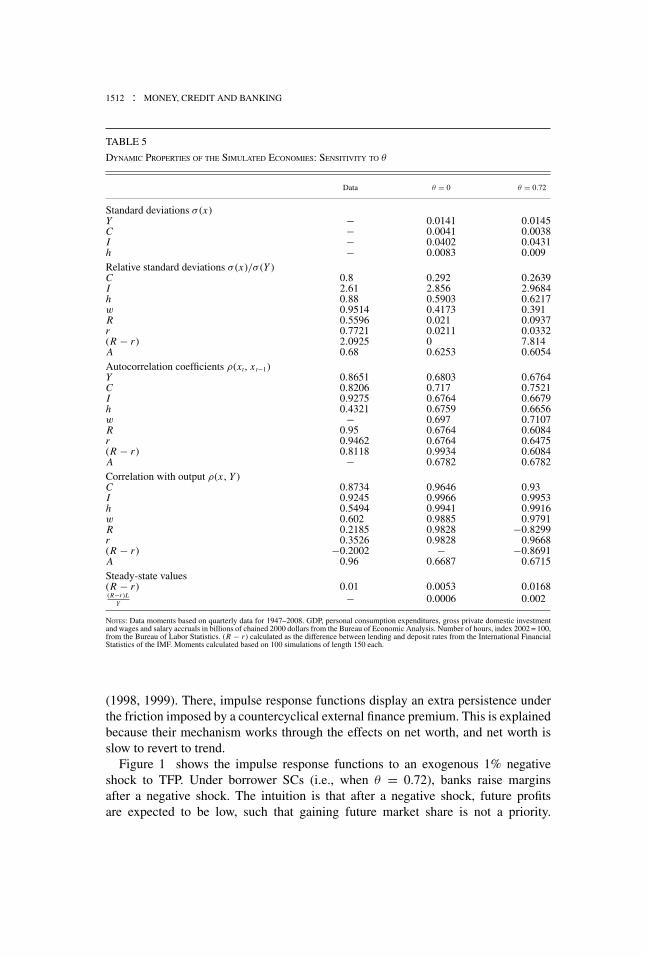
DYNAMIC PROPERTIES OF THE SIMULATED ECONOMIES: SENSITIVITY TO θ

Data θ = 0 θ = 0.72

Standard deviations σ (x)Y − 0.0141 0.0145C − 0.0041 0.0038I − 0.0402 0.0431h − 0.0083 0.009Relative standard deviations σ (x)/σ (Y )C 0.8 0.292 0.2639I 2.61 2.856 2.9684h 0.88 0.5903 0.6217w 0.9514 0.4173 0.391R 0.5596 0.021 0.0937r 0.7721 0.0211 0.0332(R − r ) 2.0925 0 7.814A 0.68 0.6253 0.6054Autocorrelation coefficients ρ(xt, xt−1)Y 0.8651 0.6803 0.6764C 0.8206 0.717 0.7521I 0.9275 0.6764 0.6679h 0.4321 0.6759 0.6656w − 0.697 0.7107R 0.95 0.6764 0.6084r 0.9462 0.6764 0.6475(R − r ) 0.8118 0.9934 0.6084A − 0.6782 0.6782Correlation with output ρ(x , Y )C 0.8734 0.9646 0.93I 0.9245 0.9966 0.9953h 0.5494 0.9941 0.9916w 0.602 0.9885 0.9791R 0.2185 0.9828 −0.8299r 0.3526 0.9828 0.9668(R − r ) −0.2002 − −0.8691A 0.96 0.6687 0.6715Steady-state values(R − r ) 0.01 0.0053 0.0168(R−r )L

Y− 0.0006 0.002

NOTES: Data moments based on quarterly data for 1947–2008. GDP, personal consumption expenditures, gross private domestic investmentand wages and salary accruals in billions of chained 2000 dollars from the Bureau of Economic Analysis. Number of hours, index 2002 = 100,from the Bureau of Labor Statistics. (R − r ) calculated as the difference between lending and deposit rates from the International FinancialStatistics of the IMF. Moments calculated based on 100 simulations of length 150 each.

(1998, 1999). There, impulse response functions display an extra persistence underthe friction imposed by a countercyclical external finance premium. This is explainedbecause their mechanism works through the effects on net worth, and net worth isslow to revert to trend.

Figure 1 shows the impulse response functions to an exogenous 1% negativeshock to TFP. Under borrower SCs (i.e., when θ = 0.72), banks raise marginsafter a negative shock. The intuition is that after a negative shock, future profitsare expected to be low, such that gaining future market share is not a priority.


FIG. 1. Impulse Response Functions: Sensitivity to θ .

NOTE: Values are percentage deviations from the steady state.


TABLE 6

DYNAMIC PROPERTIES OF THE SIMULATED ECONOMIES: SENSITIVITY TO PERSISTENCE OF HABITS AS MEASURED BY

ρs

Persistence

None Low Intermediate HighData ρs = 0 ρs = 0.5 ρs = 0.85 ρs = 0.95

Standard deviations (σ )Y − 0.0143 0.0143 0.0145 0.0146C − 0.004 0.004 0.0038 0.0037I − 0.0415 0.0418 0.0431 0.0437h − 0.0087 0.0087 0.009 0.0092Relative standard deviations σ (x)/σ (Y )C 0.8 0.2815 0.2785 0.2639 0.2549I 2.61 2.9078 2.9204 2.9684 2.9885h 0.88 0.6073 0.6086 0.6217 0.6267w 0.9514 0.4058 0.4037 0.391 0.3842R 0.5596 0.0631 0.0637 0.0937 0.1085r 0.7721 0.0716 0.0423 0.0332 0.0287(R − r ) 2.0925 33.7558 8.5896 7.814 8.0926A 0.68 0.6155 0.6141 0.6054 0.602Autocorrelation coefficients ρ(xt, xt−1)Y 0.8651 0.6563 0.6677 0.6764 0.6797C 0.8206 0.7844 0.7664 0.7521 0.7398I 0.9275 0.6249 0.65 0.6679 0.6747h 0.4321 0.6095 0.6426 0.6656 0.6741w − 0.7302 0.7189 0.7107 0.7048R 0.95 −0.1295 0.3296 0.6084 0.666r 0.9462 −0.0623 0.4402 0.6475 0.6735(R − r ) 0.8118 −0.155 0.31 0.6084 0.6625A − 0.6782 0.6782 0.6782 0.6782Correlation with outputρ(x , Y )C 0.8734 0.9354 0.9386 0.93 0.9353I 0.9245 0.9951 0.9954 0.9953 0.9958h 0.5494 0.9908 0.9914 0.9916 0.9928w 0.602 0.9796 0.9808 0.9791 0.9813R 0.2185 −0.1152 −0.3837 −0.8299 −0.9659r 0.3526 0.6454 0.8728 0.9668 0.983(R − r ) −0.2002 −0.3703 −0.6087 −0.8691 −0.9541A 0.96 0.6705 0.671 0.6715 0.6702Steady-state values(R − r ) 0.01 0.0053 0.0121 0.0168 0.0181(R−r )L

Y− 0.0006 0.0014 0.002 0.0021

NOTES: Data moments based on quarterly data for 1947–2008. GDP, personal consumption expenditures, gross private domestic investment,and wages and salary accruals in billions of chained 2000 dollars from the Bureau of Economic Analysis. Number of hours, index 2002 = 100,from the Bureau of Labor Statistics. (R − r ) calculated as the difference between lending and deposit rates from the International FinancialStatistics of the IMF. Simulations performed for a value of θ = 0.72 and η = 190. Moments calculated based on 100 simulations of length150 each.

The current profits motive dominates over the future market share motive and banksraise margins to increase their current revenues (they are able to do so becausethe short-run interest rate elasticity of the demand for credit falls with anegativeshock). Therefore, the cost of credit increases, and investment falls by more thanin the standard model with θ = 0. Because of the negative effect of this reductionin investment on the stock of capital and on the marginal productivity of labor,


FIG. 2. Cyclicality of Margins and the Persistence of Hold-Up.

NOTES: Correlation coefficients between margins and output computed from 100 model simulations of length 150 eachfor each value of the persistence parameter ρs measured on the horizontal axis.

employment and output also fall by more under hold-up than in the standard model.Resources are reallocated away from investment into consumption, such that thenegative effect on the latter is smaller when margins are countercyclical.

Thus, we provide a positive answer to the question of whether introducing acountercyclical wedge in the market for credit implies the presence of a financial ac-celerator. That is, endogenous developments in credit markets, in the pricing policiesof banks in particular, amplify and propagate the standard effects of aggregate TFPshocks. Countercyclical price-cost margins make aggregate shocks have larger realeffects than in a model that lacks this friction, and the variables of interest displaymore amplitude. Therefore, the friction introduced by borrower hold-up effects canbe interpreted as an alternative to the financial accelerator in Bernanke, Gertler, andGilchrist (BGG) (1998, 1999). While their accelerator originates in the demand sideof the market for credit (it is caused by a friction related to the value of borrowers’collateral), our accelerator is related to the supply side of the market in the sense thatdeep habits lead to banks’ pricing policies that are optimally countercyclical.

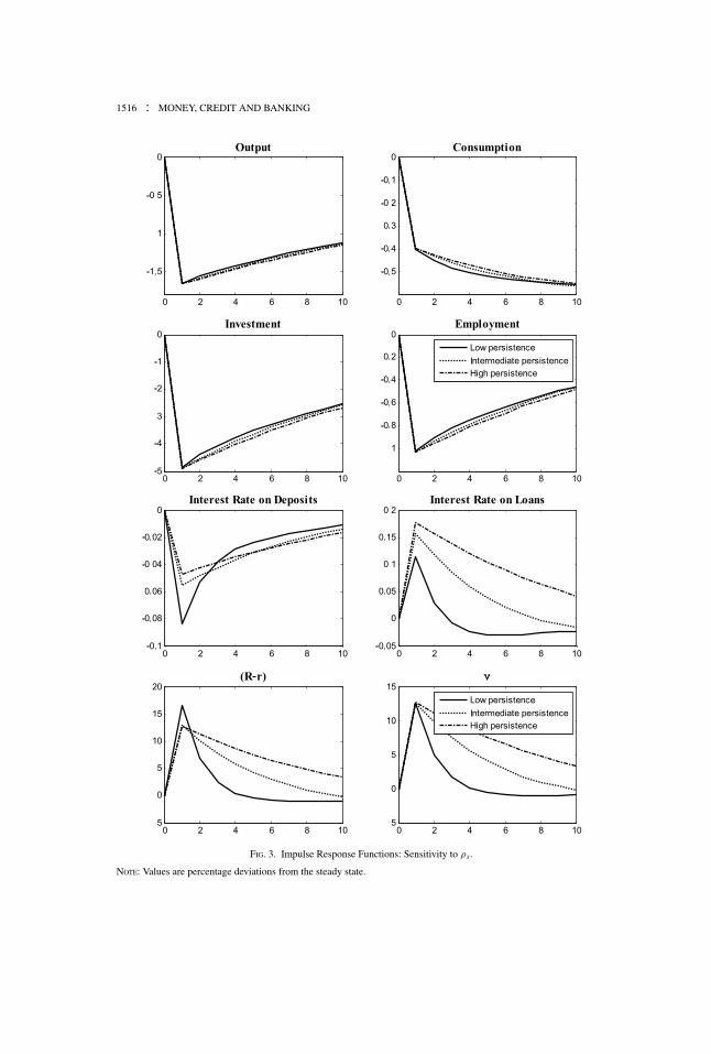
In Table 6 and Figures 2 and 3, we study the sensitivity of the dynamic prop-erties of the model to changes in the duration of the hold-up effects, as measuredby the parameter ρs. From this exercise, we can conclude that the dynamic prop-erties of the model are monotonic in ρs. Figure 2 shows that as ρs increases, mar-gins become more countercyclical. The degree of countercyclicality of margins ob-served for U.S. data can be reproduced in the presence of the estimated SCs andfor a very low persistence of the borrower hold-up effect (i.e., for θ = 0.72 andρs → 0).

The impulse responses to a 1% negative TFP shock in Figure 3 also show thatcountercyclical margins work as an amplifier of macroeconomic shocks, with thereal effects of these shocks being larger the more sensitive margins are to GDP.Although the difference in the responses of variables among alternative values


FIG. 3. Impulse Response Functions: Sensitivity to ρs.

NOTE: Values are percentage deviations from the steady state.


of the persistence parameter ρs is not quantitatively large, it is still qualitativelyimportant.

The intuition for this result is as follows. As the persistence of firm–bank rela-tionships (as measured by ρs) increases, the hold-up becomes stronger and SCs rise.Banks know that the customers that they are able to lure today will become “locked”in that relationship for several periods (for longer the larger ρs). Therefore, they facestronger incentives to change margins after an aggregate shock, and the resultingchange in the cost of credit is larger. Consequently, the responses of consumption,investment, employment, and output are all increasing in ρs.

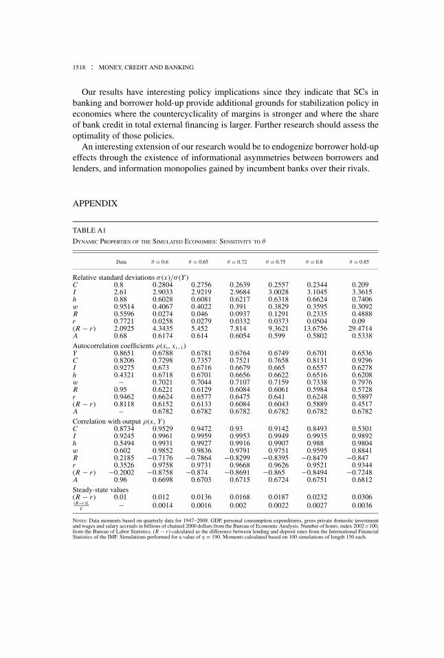
All results are qualitatively robust to the choice of parameter values in the specificsense that θ > 0 always allows us to reproduce the countercyclicality of marginsobserved in the data and that countercyclical margins always act as a financial ac-celerator that amplifies and propagates the effects of aggregate shocks (i.e., it isalways the case that in the simulated economies macroeconomic variables are morevolatile than with constant margins). In Tables A1 and A2 of the Appendix we presentconsistent results obtained for several values of θ and η. Notice that the degree ofcountercyclicality falls as θ rises. We would initially expect more strongly cyclicalmargins as the size of the friction increases. However, it is also evident from theresults in Table A1 that the level of margins themselves rises with θ , and it is a knownfeature of models with imperfect competition that the countercyclicality of marginsis decreasing in their level. This is also evident from the sensitivity analysis on η. Asη rises, margins fall at the same time that they become increasingly countercyclical(see Table A2). Results for alternative parametrizations of the model are availablefrom the authors upon request.

4. CONCLUSIONS

In this paper, we study the macroeconomic consequences of endogenously cyclicalprice-cost margins in banking. In particular, we assess their “financial accelerator”role as a propagation mechanism of macroeconomic shocks. Building on recentempirical evidence, we model this cyclicality as arising from a borrower hold-upeffect and borrower SCs by developing an application of the deep habits model ofRSGU to financial markets.

Our model allows us to reproduce two important features of business cycles thatmodels that lack this friction are unable to address: the countercyclicality of creditmargins and the fact that their volatility exceeds that of output.

Furthermore, in the simulated economies, aggregate TFP shocks trigger a changein the cost of credit, and this gives rise to two main results. First, aggregate TFPshocks have larger real effects the stronger the friction implied by borrower SCs.Second, output, investment, and employment all become more volatile than in astandard model with constant margins in credit markets. These results allow us toconclude that countercyclical price-cost margins act as a financial accelerator in theU.S. economy.


Our results have interesting policy implications since they indicate that SCs inbanking and borrower hold-up provide additional grounds for stabilization policy ineconomies where the countercyclicality of margins is stronger and where the shareof bank credit in total external financing is larger. Further research should assess theoptimality of those policies.

An interesting extension of our research would be to endogenize borrower hold-upeffects through the existence of informational asymmetries between borrowers andlenders, and information monopolies gained by incumbent banks over their rivals.

APPENDIX

TABLE A1

DYNAMIC PROPERTIES OF THE SIMULATED ECONOMIES: SENSITIVITY TO θ

Data θ = 0.6 θ = 0.65 θ = 0.72 θ = 0.75 θ = 0.8 θ = 0.85

Relative standard deviations σ (x)/σ (Y )C 0.8 0.2804 0.2756 0.2639 0.2557 0.2344 0.209I 2.61 2.9033 2.9219 2.9684 3.0028 3.1045 3.3615h 0.88 0.6028 0.6081 0.6217 0.6318 0.6624 0.7406w 0.9514 0.4067 0.4022 0.391 0.3829 0.3595 0.3092R 0.5596 0.0274 0.046 0.0937 0.1291 0.2335 0.4888r 0.7721 0.0258 0.0279 0.0332 0.0373 0.0504 0.09(R − r ) 2.0925 4.3435 5.452 7.814 9.3621 13.6756 29.4714A 0.68 0.6174 0.614 0.6054 0.599 0.5802 0.5338Autocorrelation coefficients ρ(xt, xt−1)Y 0.8651 0.6788 0.6781 0.6764 0.6749 0.6701 0.6536C 0.8206 0.7298 0.7357 0.7521 0.7658 0.8131 0.9296I 0.9275 0.673 0.6716 0.6679 0.665 0.6557 0.6278h 0.4321 0.6718 0.6701 0.6656 0.6622 0.6516 0.6208w − 0.7021 0.7044 0.7107 0.7159 0.7338 0.7976R 0.95 0.6221 0.6129 0.6084 0.6061 0.5984 0.5728r 0.9462 0.6624 0.6577 0.6475 0.641 0.6248 0.5897(R − r ) 0.8118 0.6152 0.6133 0.6084 0.6043 0.5889 0.4517A − 0.6782 0.6782 0.6782 0.6782 0.6782 0.6782Correlation with output ρ(x , Y )C 0.8734 0.9529 0.9472 0.93 0.9142 0.8493 0.5301I 0.9245 0.9961 0.9959 0.9953 0.9949 0.9935 0.9892h 0.5494 0.9931 0.9927 0.9916 0.9907 0.988 0.9804w 0.602 0.9852 0.9836 0.9791 0.9751 0.9595 0.8841R 0.2185 −0.7176 −0.7864 −0.8299 −0.8395 −0.8479 −0.847r 0.3526 0.9758 0.9731 0.9668 0.9626 0.9521 0.9344(R − r ) −0.2002 −0.8758 −0.874 −0.8691 −0.865 −0.8494 −0.7248A 0.96 0.6698 0.6703 0.6715 0.6724 0.6751 0.6812Steady-state values(R − r ) 0.01 0.012 0.0136 0.0168 0.0187 0.0232 0.0306(R−r )L

Y− 0.0014 0.0016 0.002 0.0022 0.0027 0.0036

NOTES: Data moments based on quarterly data for 1947–2008. GDP, personal consumption expenditures, gross private domestic investmentand wages and salary accruals in billions of chained 2000 dollars from the Bureau of Economic Analysis. Number of hours, index 2002 = 100,from the Bureau of Labor Statistics. (R − r ) calculated as the difference between lending and deposit rates from the International FinancialStatistics of the IMF. Simulations performed for a value of η = 190. Moments calculated based on 100 simulations of length 150 each.


TABLE A2

DYNAMIC PROPERTIES OF THE SIMULATED ECONOMIES: SENSITIVITY TO η

Data η = 130 η = 150 η = 170 η = 190 η = 210 η = 230 η = 250

Relative standard deviations σ (x)/σ (Y )C 0.8 0.2521 0.257 0.2609 0.2639 0.2665 0.2686 0.2704I 2.61 3.0261 3.0015 2.9829 2.9684 2.9568 2.9473 2.9394h 0.88 0.6369 0.6304 0.6255 0.6217 0.6186 0.6161 0.614w 0.9514 0.379 0.3841 0.388 0.391 0.3935 0.3956 0.3973R 0.5596 0.1478 0.1248 0.1074 0.0937 0.0827 0.0737 0.0662r 0.7721 0.0396 0.0368 0.0348 0.0332 0.0319 0.0309 0.0301(R − r ) 2.0925 7.9953 7.9176 7.8593 7.814 7.7779 7.7483 7.7236A 0.68 0.5959 0.5999 0.603 0.6054 0.6073 0.6089 0.6102Autocorrelation coefficients ρ(xt, xt−1)Y 0.8651 0.6741 0.6751 0.6758 0.6764 0.6768 0.6771 0.6774C 0.8206 0.7735 0.764 0.7572 0.7521 0.7481 0.745 0.7424I 0.9275 0.6633 0.6653 0.6667 0.6679 0.6687 0.6695 0.67h 0.4321 0.6603 0.6626 0.6643 0.6656 0.6667 0.6675 0.6682w − 0.7188 0.7153 0.7127 0.7107 0.7092 0.708 0.707R 0.95 0.6049 0.6064 0.6075 0.6084 0.6091 0.6098 0.6104r 0.9462 0.6378 0.6418 0.6449 0.6475 0.6497 0.6515 0.6531(R − r ) 0.8118 0.604 0.6059 0.6073 0.6084 0.6092 0.6099 0.6105A − 0.6782 0.6782 0.6782 0.6782 0.6782 0.6782 0.6782Correlation with output ρ(x , Y )C 0.8734 0.9049 0.9164 0.9242 0.93 0.9343 0.9377 0.9404I 0.9245 0.9946 0.9949 0.9952 0.9953 0.9955 0.9956 0.9957h 0.5494 0.9902 0.9908 0.9912 0.9916 0.9918 0.9921 0.9922w 0.602 0.9727 0.9756 0.9776 0.9791 0.9802 0.9811 0.9818R 0.2185 −0.8423 −0.8387 −0.8345 −0.8299 −0.8249 −0.8194 −0.8135r 0.3526 0.9604 0.963 0.9651 0.9668 0.9682 0.9694 0.9704(R − r ) −0.2002 −0.8665 −0.8676 −0.8684 −0.8691 −0.8696 −0.87 −0.8704A 0.96 0.6729 0.6723 0.6719 0.6715 0.6712 0.671 0.6708Steady-state values(R − r ) 0.01 0.0245 0.0213 0.0188 0.0168 0.0152 0.0139 0.0128(R−r )L

Y− 0.0029 0.0025 0.0022 0.002 0.0018 0.0016 0.0015

NOTES: Data moments based on quarterly data for 1947–2008. GDP, personal consumption expenditures, gross private domestic investmentand wages and salary accruals in billions of chained 2000 dollars from the Bureau of Economic Analysis. Number of hours, index 2002 = 100,from the Bureau of Labor Statistics. (R − r ) calculated as the difference between lending and deposit rates from the International FinancialStatistics of the IMF. Simulations performed for a value of θ = 0.72. Moments calculated based on 100 simulations of length 150 each.

LITERATURE CITED

Aliaga-Dıaz, R., and M. Olivero. (2008) “Macroeconomic Implications of Asymmetric Infor-mation in Banking.” Mimeo, Drexel University.

Aliaga-Dıaz, R., and M. Olivero. (2010) “Is There a Financial Accelerator in US Banking?Evidence from the Cyclicality of Banks’ Price-Cost Margins.” Economics Letters, 108,167–71.

Aliaga-Dıaz, R., and M. Olivero. (Forthcoming) “The Cyclicality of Price-Cost Margins inBanking: An Empirical Analysis of its Determinants.” Economic Inquiry.

Bernanke, B., and M. Gertler. (1989) “Agency Costs, Net Worth, and Business Fluctuations.”American Economic Review, 79, 14–31.


Bernanke, B., M. Gertler, and S. Gilchrist. (1998) “The Financial Accelerator in a QuantitativeBusiness Cycle Framework.” NBER Working Paper No. 6455.

Bernanke, B., M. Gertler, and S. Gilchrist. (1999) “The Financial Accelerator in a QuantitativeBusiness Cycle Framework.” In Handbook of Macroeconomics, edited by J. B. Taylor andM. Woodford, pp. 1341–393. New York: Elsevier

Bolton, P., and D.S. Scharfstein. (1996) “Optimal Debt Structure and the Number of Creditors.”Journal of Political Economy, 104, 1–25.

Cohen, A., and M. Mazzeo. (2004) “Competition, Product Differentiation and Quality Provi-sion: An Empirical Equilibrium Analysis of Bank Branching Decisions.” Working Paper.

Cooley, T., and E. Prescott. (1995) “Economic Growth and Business Cycles.” In Frontiers ofBusiness Cycle Research, edited by T. Cooley. Princeton, NJ: Princeton University Press.

Dell’Ariccia, G. (2001) “Asymmetric Information and the Structure of the Banking Industry.”European Economic Review, 45, 1957–80.

den Haan, W. (2000) “The Comovement between Output and Prices.” Journal of MonetaryEconomics, 46, 3–30.

Detragiache, E., P.G. Garella, and L. Guiso. (1999) “Multiple versus Single Banking Relation-ships: Theory and Evidence.” Journal of Finance, 55, 1133–61.

Diamond, D. (1984) “Financial Intermediation and Delegated Monitoring.” Review of Eco-nomic Studies, 51, 393–414.

Dueker, M., and D. Thornton. (1997) “Do Bank Loan Rates Exhibit a Countercyclical Mark-up?” Working Paper No. 1997-004A, Federal Reserve Bank of St. Louis.

Fama, E. (1985) “What’s Different about Banks?” Journal of Monetary Economics, 15, 5–29.

Hale, G., and J. Santos. (2009) “Do Banks Price Their Informational Monopoly?” Journal ofFinancial Economics, 93, 185–206.

Hart, O.D. (1995) Firms, Contracts, and Financial Structure. Oxford, UK: Oxford UniversityPress.

Kim, M., D. Kliger, and B. Vale. (2003) “Estimating Switching Costs: The Case of Banking.”Journal of Financial Intermediation, 12, 25–56.

Kim, M., E. Kristiansen, and B. Vale. (2005) “Endogenous Product Differentiation in CreditMarkets: What Do Borrowers Pay for?” Journal of Banking and Finance, 29, 681–99.

Klemperer, P. (1995) “Competition When Consumers Have Switching Costs: An Overviewwith Applications to Industrial Organization, Macroeconomics, and International Trade.”Review of Economic Studies, 62, 515–39.

Mandelman, F. (2006) “Business Cycles: A Role for Imperfect Competition in the BankingSystem.” Working Paper No. 2006-21, Federal Reserve Bank of Atlanta.

Nakamura, E., and J. Steinsson. (2006) “Price Setting in Forward-Looking Customer Markets.”Working Paper, Harvard University.

Neuberger, D., and C. Schacht. (2005) “The Number of Bank Relationships of SMEs: ADisaggregated Analysis for the Swiss Loan Market.” Working Paper No. 52, Thunen-Seriesof Applied Economic Theory.

Northcott, C. (2004) “Competition in Banking: A Review of the Literature.” Working PaperNo. 2004-24, Bank of Canada.

Olivero, M. (2010) “Market Power in Banking, Countercyclical Margins and the InternationalTransmission of Business Cycles.” Journal of International Economics, 80, 292–301.


Olivero, M., and Y. Yuan. (2009) “Switching Costs for Bank-Dependent Borrowers and theBank Lending Channel of Monetary Policy.” Mimeo, Drexel University.

Ongena, S., and D.C. Smith. (2000a) “What Determines the Number of Bank Relationships:Cross-Country Evidence.” Journal of Financial Intermediation, 9, 26–56.

Ongena, S., and D.C. Smith. (2000b) “Bank Relationships: A Survey.” In The Performance ofFinancial Institutions, edited by P. Harker and S. A. Zenios, pp. 221–58. Cambridge, UK:Cambridge University Press.

Ongena, S., and D.C. Smith. (2001) “The Duration of Bank Relationships.” Journal of Finan-cial Economics, 61, 449–75.

Petersen, M.A., and R. Rajan. (1994) “The Benefits of Lending Relationships: Evidence fromSmall Business Data.” Journal of Finance, 49, 3–37.

Rajan, R.G. (1992) “Insiders and Outsiders: The Choice Between Informed and Arm’s-LengthDebt.” Journal of Finance, 47, 1367–1400.

Ravn, M., S. Schmitt-Grohe, and M. Uribe. (2004) “Deep Habits.” NBER Working Paper No.10261.

Ravn, M., S. Schmitt-Grohe, and M. Uribe. (2006) “Deep Habits.” Review of Economic Studies,73, 195–218.

Salop, S. (1979) “Monopolistic Competition with Outside Goods.” Bell Journal of Economics,10, 141–56.

Santos, J., and A. Winton. (2008) “Bank Loans, Bonds, and Information Monopolies acrossthe Business Cycle.” Journal of Finance, 63, 1315–59.

Sharpe, S.A. (1990) “Asymmetric Information, Bank Lending and Implicit Contracts: A Styl-ized Model of Customer Relationships.” Journal of Finance, 45, 1069–87.

von Thadden, E.L. (1995) “Long-term Contracts, Short-Term Investment, and Monitoring.”Review of Economic Studies, 62, 557–75.

Vulpes, G. (2005) “Multiple Bank Lending Relationships in Italy: Their Determinants andthe Role of Firms’ Governance Features.” Working Paper, Research Department UniCreditBanca d’Impresa.

Yuan, Y. (2009) “Switching Costs for Borrowers and Macroeconomic Performance.” Mimeo,Drexel University.

Documents

Macroeconomic Implications of “Deep Habits” in Banking