Machine Learning - cdn.ttgtmedia.com Methods for Cyber... · directed acyclic graphs, have mathematical properties for characterizing rela- tionships between dynamic event and system

CHAPTER 6

Machine Learning

Machine learning is a computational process to discover the underlying mod-els of system behavior. Machine learning takes datasets, processes them, andattempts to discover causal variables. Machine learning techniques were bigin the 1980s during the first artificial intelligence. Machine learning is havinga major resurgence in the last decade because of the immense amounts ofdata available and the significant advancements in computational power.

The absence of a robust and unified theory of cyber dynamics presents chal-lenges and opportunities for using machine learning�based data-drivenapproaches to further the understanding of the behavior of such complex sys-tems. Analysts can also use machine learning approaches to gain operationalinsights. In order to be operationally beneficial, cyber security machinelearning�based models need to have the ability to: (1) represent a real-world system, (2) infer system properties, and (3) learn and adapt based onexpert knowledge and observations. Probabilistic models and probabilisticgraphical models provide these necessary properties and are further exploredin this chapter. Bayesian networks (BNs) and hidden Markov models (HMMs)are introduced as an example of a widely used data-driven classification/modeling strategy.

This chapter is organized as follows: We begin with an introduction ofmachine learning concepts and techniques. This is followed by a discussionof validating models derived through machine learning. Finally, we willexplore using BNs and HMMs.

CHAPTER OBJECTIVES

� Introduce machine learning� Discuss model validation� Explore the use of Bayesian networks and hidden Markov models in

cyber security research

Research Methods for Cyber Security. DOI: http://dx.doi.org/10.1016/B978-0-12-805349-2.00006-6© 2017 Elsevier Inc. All rights reserved. PNNL under Contract No. DE AC05-76RL01830.

153

WHAT IS MACHINE LEARNING

Machine learning is a field of study that looks at using computational algo-rithms to turn empirical data into usable models. The machine learning fieldgrew out of traditional statistics and artificial intelligences communities.From the efforts of mega corporations such as Google, Microsoft, Facebook,Amazon, and so on, machine learning has become one of the hottest compu-tational science topics in the last decade. Through their business processesimmense amounts of data have been and will be collected. This has providedan opportunity to re-invigorate the statistical and computational approachesto autogenerate useful models from data.

Machine learning algorithms can be used to (a) gather understanding of thecyber phenomenon that produced the data under study, (b) abstract theunderstanding of underlying phenomena in the form of a model, (c) predictfuture values of a phenomena using the above-generated model, and(d) detect anomalous behavior exhibited by a phenomenon under observation.There are several open-source implementations of machine learning algo-rithms that can be used with either application programming interface (API)calls or nonprogrammatic applications. Examples of such implementationsinclude Weka,1 Orange,2 and RapidMiner.3 The results of such algorithmscan be fed to visual analytic tools such as Tableau4 and Spotfire5 to producedashboards and actionable pipelines.

Cyber space and its underlying dynamics can be conceptualized as a manifes-tation of human actions in an abstract and high-dimensional space. In orderto begin solving some of the security challenges within cyber space, oneneeds to sense various aspects of cyber space and collect data.6 The observa-tional data obtained is usually large and increasingly streaming in nature.Examples of cyber data include error logs, firewall logs, and network flow.

CATEGORIES OF MACHINE LEARNING

There are two dimensions around which machine learning is generally cate-gorized: the process by which it learns and the type of output or problem itattempts to solve. For the first machine learning�based solution strategiescan be broadly classified into three categories based on the mechanism usedto perform learning namely, supervised learning, semisupervised learning,and unsupervised learning.7 For the latter, machine learning algorithms canbe broken into four categories: classification, clustering, regression, andanomaly detection.

The style of learning has an impact upon the question you are trying tosolve. In some cases, you have data that you do not know the ground truth,

154 CHAPTER 6: Machine Learning

other times it is possible to label data with categories or classifications.Sometimes you know what a good result looks like but you may not knowwhat variables are important to get there. By categorizing machine learningtechniques by the learning style can help you in selecting the best approachfor your research. Table 6.1 discusses the different styles and provides a sam-ple set of machine learning algorithms.

Supervised learning involves using a labeled dataset (e.g., the outcomes areknown and labeled). Unsupervised learning is used in cases where the labelsof the data are unknown (e.g., when the outcomes are unknown, but somesimilar measure is desired). Examples of unsupervised learning approachesinclude self-organizing maps (SOMs), K-means clustering, expectation�maximization (EM), and hierarchical clustering.8 Unsupervised learningapproaches can also be used for preliminary data exploration such asclustering similar error logs entries. Results of unsupervised algorithms arefrequently visualized using visual analytic tools. An important caveat onusing an unsupervised approach is to make sure one knows the numericspace that the data encompasses as well as the type of distance measureapplied. Semisupervised approaches are a hybrid of unsupervised andsupervised approaches. Such approaches are used when only some ofthe data is unlabeled. Semisupervised approaches are used when a portionof the data is unlabeled. Such approaches can be inductive or transductive.9

While it is sometimes helpful in picking algorithms based on what type ofinput data is available, it is equally helpfully to break them out along the

Table 6.1 Learning Style Categorization of Machine Learning Algorithms

Style Definition Example Algorithms

Unsupervised In unsupervised learning, no extra or meta data isprovided to the algorithm and it is forced to discoverthe structure data and the relationship of variables byobserving a raw dataset.

K-means clustering, hierarchical clustering,principal component analysis

Supervised In supervised learning, input data is annotated withexpert information detailing what the expected outputor answer would be. The process of annotating datafor supervised learning is called labeling.

Neural network, Bayesian networks,decision tree, support vector machine

Semi-supervised

In semisupervised learning a small set of learningdata is labeled but large gaps in labeling are present.This is largely used when it is known that a smallnumber of variables led to a result, but the full extent ofthe variables involved is unknown. A special case ofsemisupervised learning is called reinforced learningwhere an expert informs the algorithm if its output iscorrect or not.

Expectation�maximization, transductivesupport vector machine, Markov decisionprocesses

Categories of Machine Learning 155

result types provided. Variables within a dataset can be numeric (i.e., discreteor continuous), ordinal (i.e., order matters), cardinal (i.e., integer valued),nominal/categorical (i.e., used as an outcome class name). Machine learningalgorithms can also be categorized based on the type of problem they solve.An example of such a breakdown of algorithms is listed in Table 6.2.

Decision tree algorithms: classification trees (e.g.,C4.5) can be used in casesof a nominal class variable while regression trees can be used for continuousnumeric valued outcome variables.

As discussed by Murphy et al.,11 several issues affect the alternative learningschemes, including:

� Dynamic range of the features� Number of features� Type of the class variable� Types of the features� Heavily correlated features

In order to be operationally beneficial, cyber security machine learning�based models need to have the ability to: (1) represent a real-world system,(2) infer system properties, and (3) learn and adapt based on expert know-ledge and observations. Probabilistic graphical models have wide applica-tions for assessing and quantifying cyber security risks.12,13 These modelscontain desirable properties including representation of a real-world system,inference about queries of interest related to the system, and learning fromexpert knowledge and past experience.14 The probabilistic terms in thesemodels may be estimated or learned from historical data, generated fromsimulation experiments, or elicited through informed judgments of subjectmatter experts.

Table 6.2 Categories of Machine Learning Algorithms Separated by Problems they Address10

Problem Definition Example Algorithms

Classification Classification algorithms take labeled data andgenerate models that classify new data into thelearned labels.

Hidden Markov models, support vectormachines (SVMs), random forests, naïve bayes,probabilistic graphical models, logisticregression, neural networks [9]

Clustering Cluster analysis attempts to take a dataset anddefine clusters of like items.

K-means, heirarchical, density-based (DBSCAN)

Regression Regression attempts to generate a predictivemodel by optimizing the error in learned data.

Linear,logistic, ordinary least squares,multivariate adaptive regression splines

Anomalydetection

Anomaly detection takes a dataset of “normal”items and learns a model of normal. This model isused to determine if any new data is anomalousor low probability of occurring.

One-class SVM, linear regression and logisticregression, frequent pattern growth (FP-growth),a priori


DID YOU KNOW?

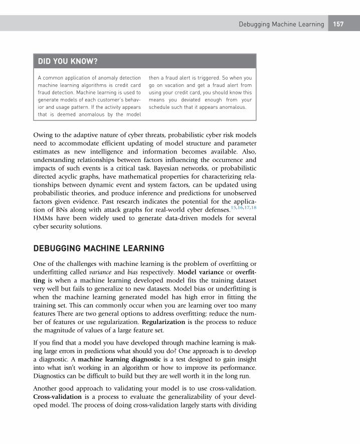
A common application of anomaly detectionmachine learning algorithms is credit cardfraud detection. Machine learning is used togenerate models of each customer’s behav-ior and usage pattern. If the activity appearsthat is deemed anomalous by the model

then a fraud alert is triggered. So when yougo on vacation and get a fraud alert fromusing your credit card, you should know thismeans you deviated enough from yourschedule such that it appears anomalous.

Owing to the adaptive nature of cyber threats, probabilistic cyber risk modelsneed to accommodate efficient updating of model structure and parameterestimates as new intelligence and information becomes available. Also,understanding relationships between factors influencing the occurrence andimpacts of such events is a critical task. Bayesian networks, or probabilisticdirected acyclic graphs, have mathematical properties for characterizing rela-tionships between dynamic event and system factors, can be updated usingprobabilistic theories, and produce inference and predictions for unobservedfactors given evidence. Past research indicates the potential for the applica-tion of BNs along with attack graphs for real-world cyber defenses.15,16,17,18

HMMs have been widely used to generate data-driven models for severalcyber security solutions.

DEBUGGING MACHINE LEARNING

One of the challenges with machine learning is the problem of overfitting orunderfitting called variance and bias respectively. Model variance or overfit-ting is when a machine learning developed model fits the training datasetvery well but fails to generalize to new datasets. Model bias or underfitting iswhen the machine learning generated model has high error in fitting thetraining set. This can commonly occur when you are learning over too manyfeatures There are two general options to address overfitting: reduce the num-ber of features or use regularization. Regularization is the process to reducethe magnitude of values of a large feature set.

If you find that a model you have developed through machine learning is mak-ing large errors in predictions what should you do? One approach is to developa diagnostic. A machine learning diagnostic is a test designed to gain insightinto what isn’t working in an algorithm or how to improve its performance.Diagnostics can be difficult to build but they are well worth it in the long run.

Another good approach to validating your model is to use cross-validation.Cross-validation is a process to evaluate the generalizability of your devel-oped model. The process of doing cross-validation largely starts with dividing

Debugging Machine Learning 157

your initial dataset into three; a training set, a cross-validation set, and a testset. You want to have a sufficient amount of data for your training set so agood rule of thumb is to make the divisions at 60% training, 20% cross vali-dation, and 20% test. The cross-validation set is used to tune or find thebest-fit model parameters. Then the test set is used to determine the gener-alizability of the generated model.

There are a few more tips for addressing. To fix high variance you can getmore training data or try to learn around a smaller set of features or vari-ables. To fix high bias try adding more features or polynomial features. Inboth cases tuning your parameters can help.

DID YOU KNOW?

In 2011 the IBM Watson super computercompeted in two Jeopardy matches withBrad Rutter and Ken Jennings, two of themost successful Jeopardy players in his-tory. The technology underlying Watson’sability to parse and answer questions,

called DeepQA, leveraged over 100 machinelearning algorithms.19 But it wasn’t just thealgorithms alone but also the pipeline andstructured sequence of using the machinelearning algorithms that helped Watsonbest two of the best Jeopardy contestants.

BAYESIAN NETWORK MATHEMATICAL PRELIMINARIESAND MODEL PROPERTIES

A BN is a graphical model that represents uncertainties (as probabilities)associated with discrete or continuous random variables (nodes) andtheir conditional dependencies (edges) within a directed acyclicgraph.20,21

BNs model the relationships among variables and may be updated as addi-tional information about these variables becomes available. Mathematically,if nodes represent a set of random variables, X5X1;X2; :::;Xn then a setof links connecting these nodes Xi-Xj represent the dependencies amongthe variables. Also, each node is conditionally independent of nondescen-dant nodes given its parent nodes and has an attached probability function.As a result, the joint probability of all nodes, P Xð Þ may be represented as:Ln

i51P�Xi j parentsðXiÞ

�.

Strengths and LimitationsKey strengths and limitations of BNs are listed below:

� Models dependencies among random variables as directed acyclic graphs� Allows probabilistic inference of unobserved variables� Graphical representation may be intuitive for users


� Incorporate data/expert judgments and update structure/parameters as“new” data/knowledge becomes available

� Inferring structure of an unknown network may be computationallydemanding from a scalability perspective

� Identifying reliable prior knowledge is a challenge

Data-driven Learning and Probabilistic Inference withinBayesian NetworksStructure learning within Directed Acyclic Graphs (DAGs) may be broadly clas-sified as: (1) constraint-based and (2) score-based. Constraint-based algorithmsuse conditional independence tests using the data to build causal graphs thatsatisfy constraints. A challenge associated with constraint-based approaches isidentifying independence properties and optimizing network structure. Also,these approaches do not account for a well-defined objective function and mayresult in nonoptimal graphical structures. Score-based algorithms assigns a scorefunction to the entire space of causal graphs and typically use greedy searchamong various potential DAGs to identify the structure with the highest score.These approaches are optimization-based and tend to scale better.

Data-driven statistical learning methods (e.g., Hill Climbing and Grow-Shrinkalgorithms) may be adopted to infer Bayesian network structures for variousparameters of interest across geographic regions. Hill Climbing is a score-based algorithm that uses greedy heuristic search to maximize scores assignedto candidate networks.22 Grow-Shrink is a constraint-based algorithm thatuses conditional independence tests to detect blankets (comprised of a node’sparents, children, and children’s other parents) of various variables.

DIG DEEPER: BAYESIAN NETWORK PROVENANCEThe probabilities and process underlying BNs was first defined by Thomas Bayes in mid-17th century. The Bayes rule determines the probability of an event by updating prior proba-bilities with new information. It wasn’t until the 1980s that Judea Pearl made the distinctionbetween evidence and causality. In the Bayesian network defined by Pearl, the nature anduncertainty of evidence is taken into account before updating probabilities.

Parameter LearningProbabilistic parameters associated with these network structures may be esti-mated using expectation maximization and maximum likelihood estimation tech-niques. Expectation maximization is useful with not fully observed data,and is an iterative algorithm where in the “Expectation” step the probabilityof unobserved variables given observed and current parameters are estimated.Thereafter, in the “Maximization” step the current parameters are updatedthrough log-likelihood maximization.

Bayesian Network Mathematical Preliminaries and Model Properties 159

Maximum likelihood approach is useful with fully observed data andinvolves estimating probabilistic parameters θ, for each node in the graphsuch that the log-likelihood function, log

�PðXjθÞ�, is maximized.

Bayesian estimation is also an option, where θ is treated as a random vari-able, a prior probability p θð Þ is assumed, and data is used to estimate theposterior probability of pðθjXÞ.

Probabilistic InferenceBNs apply Bayes’ theorem for inference of unobserved variables. Variableelimination (by integration or summation) of unobserved, nonquery vari-ables is a widely used exact inference method. Approximate inference meth-ods include stochastic Markov Chain monte Carlo (MCMC) simulation, logicsampling, likelihood weighting, and others.

Notional Example with bnlearn Package in RR, in conjunction with the RStudio integrated development environment,provides a powerful platform for data analysis. The default setup of R pro-vides several libraries including the stat library. R and RStudio need to beinstalled separately.23,24 The example described below uses the R package“bnlearn”25 for structure learning, parameter learning, and probabilistic infer-ence. The code begins by loading the “learning” dataset. This data has dis-crete levels for each of the following random variables: In a realistic cybersetting, these random variables (e.g., A, B, etc.) may represent the time-varying health of system components and the levels (e.g., a, b, c) may repre-sent the discrete states of health.

#install.packages(“bnlearn”)library(bnlearn)data(learning.test)str(learning.test)## ‘data.frame’: 5000 obs. of 6 variables:## $ A: Factor w/ 3 levels “a”,“b“,”c”: 2 2 1 1 1 3 3 2 2 2 . . .

## $ B: Factor w/ 3 levels “a”,”b”,”c”: 3 1 1 1 1 3 3 2 2 1 . . .

## $ C: Factor w/ 3 levels “a”,”b”,”c”: 2 3 1 1 2 1 2 1 2 2 . . .

## $ D: Factor w/ 3 levels “a”,”b”,”c”: 1 1 1 1 3 3 3 2 1 1 . . .

## $ E: Factor w/ 3 levels “a”,”b”,”c”: 2 2 1 2 1 3 3 2 3 1 . . .

## $ F: Factor w/ 2 levels “a”,”b”: 2 2 1 2 1 1 1 2 1 1 . . .

head(learning.test)## A B C D E F## 1 b c b a b b## 2 b a c a b b## 3 a a a a a a## 4 a a a a b b## 5 a a b c a a## 6 c c a c c a


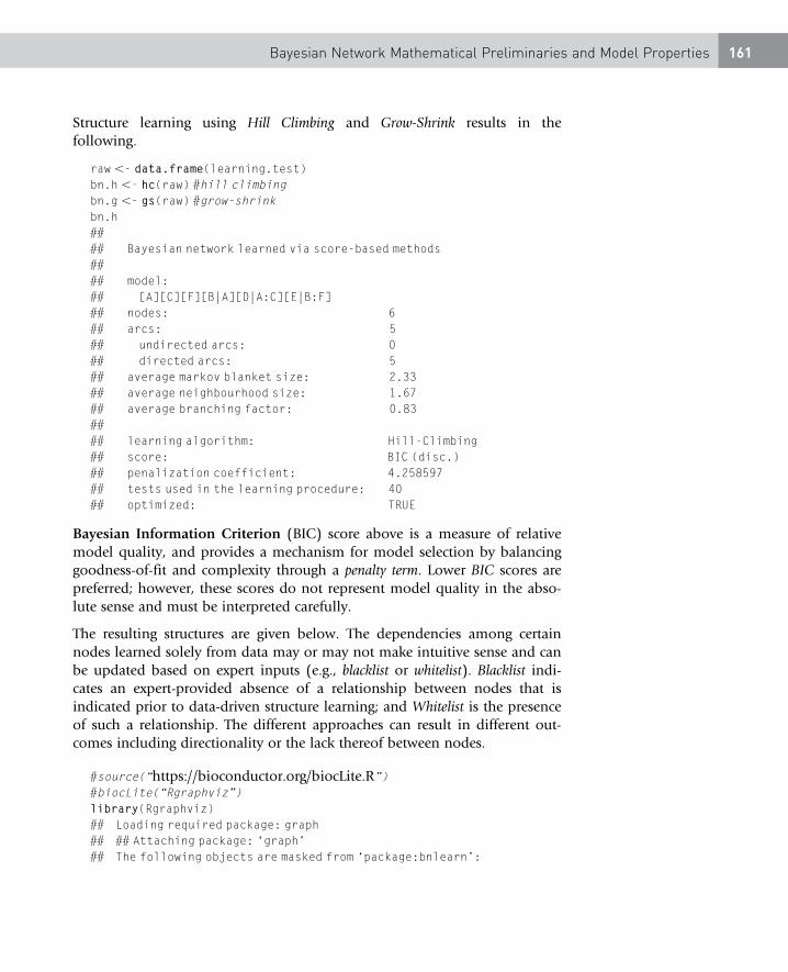
Structure learning using Hill Climbing and Grow-Shrink results in thefollowing.

raw ,- data.frame(learning.test)bn.h ,- hc(raw) #hill climbingbn.g ,- gs(raw) #grow-shrinkbn.h#### Bayesian network learned via score-based methods#### model:## [A][C][F][B|A][D|A:C][E|B:F]## nodes: 6## arcs: 5## undirected arcs: 0## directed arcs: 5## average markov blanket size: 2.33## average neighbourhood size: 1.67## average branching factor: 0.83#### learning algorithm: Hill-Climbing## score: BIC (disc.)## penalization coefficient: 4.258597## tests used in the learning procedure: 40## optimized: TRUE

Bayesian Information Criterion (BIC) score above is a measure of relativemodel quality, and provides a mechanism for model selection by balancinggoodness-of-fit and complexity through a penalty term. Lower BIC scores arepreferred; however, these scores do not represent model quality in the abso-lute sense and must be interpreted carefully.

The resulting structures are given below. The dependencies among certainnodes learned solely from data may or may not make intuitive sense and canbe updated based on expert inputs (e.g., blacklist or whitelist). Blacklist indi-cates an expert-provided absence of a relationship between nodes that isindicated prior to data-driven structure learning; and Whitelist is the presenceof such a relationship. The different approaches can result in different out-comes including directionality or the lack thereof between nodes.

#source(“https://bioconductor.org/biocLite.R”)#biocLite(“Rgraphviz”)library(Rgraphviz)## Loading required package: graph## ## Attaching package: ‘graph’## The following objects are masked from ‘package:bnlearn’:


#### degree, nodes, nodes,-## Loading required package: gridpar(mfrow 5 c(1, 2))graphviz.plot(bn.h, main 5 “Hill climbing”)graphviz.plot(bn.g, main 5 “Grow-shrink”)

In this notional example, the hill climbing and grow-shrink-based BN structuresabove are similar except the directionality between nodes A and B. Grow-shrink results in an undirected edge between nodes A and B, whereas hillclimbing results in the learning of a dependence of node B on node A. Oncethe network structure is determined, one can learn the model parameters(i.e., conditional probability tables (CPT) for the discrete case) associated witheach node in the BN. The results below display parameters of node D basedon maximum likelihood and Bayesian estimation methods.

fit.bnm ,- bn.fit(bn.h, data 5 raw, method 5 “mle”)fit.bnm$D#### Parameters of node D (multinomial distribution)#### Conditional probability table:#### , , C 5 a#### A## D a b c## a 0.80081301 0.09251810 0.10530547## b 0.09024390 0.80209171 0.11173633## c 0.10894309 0.10539019 0.78295820#### , , C 5 b#### A


## D a b c## a 0.18079096 0.88304094 0.24695122## b 0.13276836 0.07017544 0.49390244## c 0.68644068 0.04678363 0.25914634#### , , C 5 c#### A## D a b c## a 0.42857143 0.34117647 0.13333333## b 0.20238095 0.38823529 0.44444444## c 0.36904762 0.27058824 0.42222222fit.bnb ,- bn.fit(bn.h, data 5 raw, method 5 “bayes”)fit.bnb$D#### Parameters of node D (multinomial distribution)#### Conditional probability table:#### , , C 5 a#### A## D a b c## a 0.80039110 0.09273317 0.10550895## b 0.09046330 0.80167307 0.11193408## c 0.10914561 0.10559376 0.78255696#### , , C 5 b#### A## D a b c## a 0.18126825 0.88126079 0.24724285## b 0.13339591 0.07102763 0.49336034## c 0.68533584 0.04771157 0.25939680#### , , C 5 c#### A## D a b c## a 0.42732811 0.34107527 0.13577236## b 0.20409051 0.38752688 0.44308943## c 0.36858138 0.27139785 0.42113821

The code below generates a plot of the CPT.

bn.fit.barchart(fit.bnm$D, xlab 5 “Probabilities”, ylab 5 “Levels”,main 5 “Conditional Probabilities”)## Loading required namespace: lattice


With the BN structure and parameters, we can perform probabilistic infer-ence. Logic sampling and likelihood weighting are currently implementedoptions. For example, P(B55 “b”| A55 “a”) B 0.025.

cpquery(fit.bnm, event5(B 55 “b”), evidence5(A 55 “a”))## [1] 0.02622852cpquery(fit.bnm, event5(B 55 “b”), evidence5(A 55 “a” & D 55 “c”))## [1] 0.02760351

BNs are also useful for in-sample and out-of-sample predictions. In-samplepredictions are useful for model evaluation and out-of-sample predictionshelp with model testing and validation. An out-of-sample prediction exam-ple is given below with training and testing datasets and out-of-sample pre-dictive performance of 90%.

train ,- raw[1:4990, ]test ,- raw[4991:5000, ]bn.train ,- hc(train)fit ,- bn.fit(bn.train, data 5 train)pred ,- predict(fit, “D”, test)#library(xtable)#print(xtable(cbind(pred, test[, “D”])), type5‘html’)#print(xtable(table(pred, test[, “D”])), type5‘html’)cbind(pred, test[, “D”])## pred


## [1,] 1 1## [2,] 3 3## [3,] 2 2## [4,] 1 2## [5,] 2 2## [6,] 1 1## [7,] 2 2## [8,] 2 2## [9,] 3 3## [10,] 1 1table(pred, test[, “D”])#### pred a b c## a 3 1 0## b 0 4 0## c 0 0 2

HIDDEN MARKOV MODELS

In this section, we discuss HMMs,26 which are a type of dynamic BN models.HMMs have found applications in biological sequence analysis for gene andprotein structure predictions,27,28,29 multistage network attack detection30,and in pattern recognition problems31 such as speech,32 handwriting,33 andgesture34 recognition. HMMs model the generation of a sequence of statesthat can only be inferred from a sequence of observed symbols. The symbolscan be discrete (e.g., events, tosses of a coin) or continuous. In a HMM, ahidden Markov process generates the sequence of states, which are in turnused to explain and characterize the occurrence of a sequence of observablesymbols. Therefore, the generation of the observable symbols is probabilisti-cally dependent on the generation of the unobservable Markov states.

To illustrate the process of generating the observation sequence in a HMM, let’sdenote a time-ordered sequence of observed symbols of length T, asY 5 fY1;Y2; . . . ;YTg, and the associated hidden sequence of Markov states, asX5 fX1;X2; . . . ;XTg. Each observed element,Yi, can be a symbol describing theoutcome of a stochastic process. Let O5 O1;O2; . . . ;OMf g represent a discreteset of M such possible outcomes (observed symbols). Similarly letS5 fS1; S2; . . . ;YNg represent a discrete set of N distinct Markov states. Besidesspecifying the number of observed symbols, M, and the number of distinctMarkov states, N, a HMM specification involves specifying three probability dis-tributions: (1) the transition state probability distribution, A; (2) the probabilitydistribution to choose the observed symbol from a state, B; and (3) the initialstate distribution, π. The compact notation, λ5 A;B;πð Þ, is normally used torepresent an HMM.

Hidden Markov Models 165

Fig. 6.1 illustrates a general example of an HMM. The process of generatingthe observation sequence is described below.

Generation of observation sequence in HMM

1. Initialize time index, t 5 12. Choose the initial state, Xt , according to the initial state distribution, π.3. Choose the observed symbol, Yt , according to the probability

distribution, B in state Xt .4. Choose a new state, Xt11according to the state transition probability

distribution, A for the current state, Xt .5. Set t5 t1 16. if t, T then7. go to step 38. end if

There are three types of problems that need to be solved, in order for HMMsto be useful in real-world applications:

� Problem 1: Given the observation sequence, Y 5 fY1;Y2; . . . ;YTg, andthe model parameters, λ5 A;B;πð Þ, compute the probability

FIGURE 6.1General process modeled by hidden Markov models.


(likelihood), PðYjλÞ; that the observed sequence was produced by themodel. Problem 1 aims to evaluate the model.

� Problem 2: Given the observation sequence, Y 5 fY1;Y2; . . . ;YTg, andthe model parameters, λ5 A;B;πð Þ, determine the most optimal statesequence of the underlying Markov process, X5 fX1;X2; . . . ;XTg.Problem 2 aims to uncover the hidden part of the model.

� Problem 3: Given the observation sequence, Y 5 fY1;Y2; . . . ;YTg, andthe dimensions M and N, adjust the parameters of the model,λ5 A;B;πð Þ, to maximize PðOjλÞ. Problem 3 aims to find the bestmodel that fits a training sequence of observed symbols.

Notional Example with HMM Package in RThis example uses the R package “HMM” for: (1) computing most probablepath of states given a HMM and (2) inferring optimal parameters to a HMM.The Viterbi algorithm for state path estimation is implemented below:

#install.packages(“HMM”)#source: https://cran.r-project.org/web/packages/HMM/HMM.pdflibrary(HMM)##Viterbi algorithm for computing most probable path of states given anHMM# HMM Initializationhmm 5 initHMM(c(“A”,”B”,”C”), c(“o1”,”o2”), startProbs5matrix(c(.25,.5,.25),1), transProbs5matrix(c(.3,.4,.6,.4,.4,.3,.3,.2,.1),3), emissionProbs5matrix(c(.5,.4,.9,.5,.6,.1),3))print(hmm)## $States## [1] “A” “B” “C”#### $Symbols## [1] “o1” “o2”#### $startProbs## A B C## 0.25 0.50 0.25#### $transProbs## to## from A B C## A 0.3 0.4 0.3## B 0.4 0.4 0.2## C 0.6 0.3 0.1#### $emissionProbs## symbols

Hidden Markov Models 167

## states o1 o2## A 0.5 0.5## B 0.4 0.6## C 0.9 0.1# Sequence of observationsobservations 5 c(“o1”,”o2”,”o2”,”o1”,”o1”,”o2”)print(observations)## [1] “o1” “o2” “o2” “o1” “o1” “o2”# Calculate Viterbi pathviterbi 5 viterbi(hmm,observations)print(viterbi)## [1] “C” “A” “B” “A” “C” “A”

The Viterbi-training algorithm for inferring optimal parameters is implemen-ted below.

##Viterbi-training algorithm for inferring optimal parameters to an HMM# Initial HMMhmm 5 initHMM(c(“A”,”B”,”C”), c(“o1”,”o2”), startProbs5matrix(c(.25,.5,.25),1), transProbs5matrix(c(.3,.4,.6,.4,.4,.3,.3,.2,.1),3), emissionProbs5matrix(c(.5,.4,.9,.5,.6,.1),3))# Sequence of observationsa 5 sample(c(rep(“o1”,100),rep(“o2”,300)))b 5 sample(c(rep(“o1”,300),rep(“o2”,100)))observation 5 c(a,b)# Viterbi-trainingvt 5 viterbiTraining(hmm,observation,1000)print(vt$hmm)## $States## [1] “A” “B” “C”#### $Symbols## [1] “o1” “o2”#### $startProbs## A B C## 0.25 0.50 0.25#### $transProbs## to## from A B C## A 0.0000000 0.2981928 0.7018072## B 0.4230769 0.5769231 0.0000000## C 1.0000000 0.0000000 0.0000000#### $emissionProbs## symbols## states o1 o2


## A 0.5 0.5## B 0.0 1.0## C 1.0 0.0

DISCUSSION

BNs and HMMs provide a probabilistic framework to infer, predict, and gaininsights into the dependencies between components within a cyber system.The choice of random variables, their types (discrete or continuous), andstate information are critical for designing and interpreting BN and HMMresults. Within BNs, the strength and direction of component dependencies(represented as conditional probabilities) learned from data may vary acrosssystems and time periods. Additional cyber intelligence information relatedto pre-event conditions and postevent impacts can be valuable for enhancingwhat-if and forensic analyses. Modeling extensions of interest may includethe use of dynamic BNs that allow evolution over time and hybrid networksthat can accommodate mixed discrete and continuous random variables asnodes. Further, validation approaches may be incorporated to test variousdata-driven learning models using appropriate training and testing datasets.

SAMPLE FORMAT

In the following, we will provide you with a general outline for publishingyour results. Every publication will provide their own formatting guidelines.Be sure to check your selected venue’s submission requirements to make sureyou follow any outline and formatting specifications. The outline providedhere follows a common flow of information found in published papers andshould meet the requirements of a larger number of publisher specifications.

Every paper is unique and requires some different ways of presentation; how-ever, the provided sample flow includes all of the general information that isimportant to cover in a paper and is a general starting format we take whenstarting to write a paper and then modify it to support the topic and venue.We understand that every researcher has their own style of presentation, sofeel free to use this as a jumping-off point. The discussions of each sectionare provided to explain what is important to include and why, so you canpresent the important information in whatever way best suits your style.

AbstractThe abstract is a concise and clear summary of the paper. The goal of anabstract is to provide readers with a quick description of what the paper dis-cusses. You should only talk about what is stated in the rest of the paper and

Sample Format 169

nothing additional. Each submission venue will provide guidelines on howto provide an abstract. Generally, this includes the maximum length of theabstract and formatting instructions, but sometimes this will include infor-mation on the type and layout of the content to provide.

IntroductionThe first section of a paper should always be an introduction for the readerinto the rest of the paper. The introduction section provides the motivationand reasoning behind why the research was performed. This should includea statement of the research question and any motivating questions that wereused for the research. If any background information is required, such asexplaining the domain, environment, or context of the research, you woulddiscuss it here. If the audience is significantly removed from some aspect ofthis topic, it may be worth it to create an independent background section.In machine learning papers, it is good to include the performance or learningcriteria around which you will determine the quality of the machine learningapplication. It’s also good to specify the category of machine learning youare describing in this paper; is it a new machine learning algorithm or anapplication of an existing machine learning approach to a new set of data?

Related WorkThe related works section should include a quick summarization of thefield’s knowledge about this research topic. Are there competing solutions?Have other machine learning approaches been used in the past? Explainwhat is deficient about past applications. What was the gap in the solutionspace that motivated the use of the proposed machine learning approachdefined in this paper.

ApproachThe approach section of an applied paper is often the meat or largest portionof the paper. In this section you describe how your machine learning algo-rithm works and represents or systematizes knowledge. Describe your learn-ing dataset and any processing or manipulation of the data to provide it tothe algorithm.

EvaluationIn the evaluation explain how you are going to exercise the machine learningapproach to generate a results dataset for performance characterization.Discuss what test datasets you will use. Explain if you do cross-validationand regularization.


Data Analysis/ResultsIn the results section of your paper, explain what you found after you per-formed your analysis. Present the performance and/or learning resultsaround whatever metrics you define. Comparative analysis with past or com-peting applied solutions are very helpful in contextualizing your results.Without previous performance numbers it is difficult to understand the sig-nificance of your work. Creating tables to show results is an efficient andeffective method. You can also show pictures of interesting results, that is if adata anomaly occurred or to display the distributions of the data samples.

Discussion/Future WorkThe discussion/future work section is for you to provide your explanationsfor the results you received. Discuss additional tests you think should be per-formed. Discuss future directions in research that may result from the know-ledge gained from the evaluation. If performance was less than expectedshould more observation research be performed?

Conclusion/SummaryIn the final section of the paper, summarize the results and conclusions ofthe paper. The conclusion section is often a place readers jump to quicklyafter reading the abstract. Make a clear and concise statement about what theultimate results of the experiments and what you learned from it.

AcknowledgmentsThe acknowledgments section is a place for you to acknowledge anyone whohelped you with parts of the research that were not part of the paper. It isalso good to acknowledge and funding sources that supported your research.

ReferencesEach publication will provide some guidelines on how to format references.Follow their guidelines and list all your references at the end of your paper.Depending on the length of the paper you will want to adjust the number ofreferences. The longer the paper the more references. A good rule of thumb is15�20 references for a 6-page paper. For peer-reviewed publications, themajority of your references should be other peer-reviewed works. Referencingweb pages and Wikipedia doesn’t generate confidence in reviewers. Also,make sure you only list references that are useful to your paper, that is don’tinflate your reference count. Good reviewers will check and this will likelydisqualify and reflect poorly on you.

Sample Format 171

Endnotes1. Weka 3: Data Mining Software in Java. (n.d.). Retrieved February 25, 2017, from http://

www.cs.waikato.ac.nz/ml/weka/Weka.2. Shaulsky, G., Borondics, F., Bellazzi, R. (n.d.). Orange—Data Mining Fruitful & Fun. Retrieved

February 25, 2017, from http://orange.biolab.si/BioLab, University of Ljubljana.3. Data Science Platform. Machine Learning (2017, February 22). Retrieved February 25, 2017,

from http://www.rapidminer.com/rapidminer.4. Tableau Software (n.d.). Retrieved February 25, 2017, from http://www.tableau.com/.5. Data Visualization & Analytics Software—TIBCO Spotfire. (n.d.). Retrieved February 25,

2017, from http://spotfire.tibco.com/.6. Sheymov, V., Cyberspace and Security: A Fundamentally New Approach. 2012: Cyber books

publishing.7. Chapelle, O., B. Schölkopf, and A. Zien, Semi-supervised Learning. 2010: MIT Press.8. Murphy, K.P., Machine Learning: A Probabilistic Perspective. 2012: MIT Press.9. Chapelle, O., B. Schölkopf, and A. Zien, Semi-supervised Learning. 2010: MIT Press.10. Borgelt, C., An implementation of the FP-growth algorithm, in Proceedings of the 1st international

workshop on open source data mining: Frequent pattern mining implementations. 2005, ACM:Chicago, Illinois, pp. 1�5.

11. Murphy, K.P., Machine Learning: A Probabilistic Perspective. 2012: MIT Press.12. Ezell, B.C., et al., Probabilistic risk analysis and terrorism risk. Risk Analysis, 2010. 30(4):

p. 575�589.13. Koller, D. and N. Friedman, Probabilistic graphical models: principles and techniques. 2009: MIT

press.14. Koller, D. and N. Friedman, Probabilistic graphical models: principles and techniques. 2009: MIT

press.15. Frigault, M., et al. Measuring network security using dynamic bayesian network. in Proceedings of

the 4th ACM workshop on Quality of protection. 2008. ACM.16. Xie, P., et al. Using Bayesian networks for cyber security analysis. in 2010 IEEE/IFIP International

Conference on Dependable Systems and Networks (DSN). 2010. IEEE.17. Bode Moyinoluwa, A., K. Alese Boniface, and F. Thompson Aderonke. A Bayesian Network

Model for Risk Management in Cyber Situation. in Proceedings of the World Congress onEngineering and Computer Science. 2014.

18. Shin, J., H. Son, and G. Heo, Development of a cyber security risk model using Bayesian networks.Reliability Engineering and System Safety, 2015. 134: p. 208�217.

19. https://www.aaai.org/Magazine/Watson/watson.php.20. Team, R.C., R: A language and environment for statistical computing. 2013.21. Nielsen, T.D. and F.V. Jensen, Bayesian Networks and Decision Graphs. 2007: Springer New

York.22. Bode Moyinoluwa, A., K. Alese Boniface, and F. Thompson Aderonke. A Bayesian Network

Model for Risk Management in Cyber Situation. in Proceedings of the World Congress onEngineering and Computer Science. 2014.

23. Team, R.C., R: A language and environment for statistical computing. 2013.24. RStudio. 2016: https://www.rstudio.com/.25. Scutari, M., Learning Bayesian networks with the bnlearn R package. arXiv preprint

arXiv:0908.3817, 2009.26. Rabiner, L.R., A Tutorial on Hidden Markov-Models and Selected Applications in Speech

Recognition. Proceedings of the Ieee, 1989. 77(2): p. 257�286.27. Yoon, B.-J., Hidden Markov models and their applications in biological sequence analysis. Current

genomics, 2009. 10(6): p. 402�415.28. Krogh, A., et al., Hidden Markov models in computational biology: Applications to protein modeling.

Journal of molecular biology, 1994. 235(5): p. 1501�1531.


29. Eddy, S.R., What is a hidden Markov model? Nature biotechnology, 2004. 22(10):p. 1315�1316.

30. Ourston, D., et al. Applications of hidden markov models to detecting multi-stage network attacks.in System Sciences, 2003. Proceedings of the 36th Annual Hawaii International Conference on.2003. IEEE.

31. Fink, G.A., Markov models for pattern recognition: from theory to applications. 2014: SpringerScience & Business Media.

32. Gales, M. and S. Young, The application of hidden Markov models in speech recognition.Foundations and trends in signal processing, 2008. 1(3): p. 195�304.

33. Plötz, T. and G.A. Fink, Markov models for offline handwriting recognition: A survey.International Journal on Document Analysis and Recognition (IJDAR), 2009. 12(4):p. 269�298.

34. Moni, M. and A.S. Ali. HMM based hand gesture recognition: A review on techniques andapproaches. in Computer Science and Information Technology, 2009. ICCSIT 2009. 2nd IEEEInternational Conference on. 2009. IEEE.

Endnotes 173

Documents

Machine Learning - cdn.ttgtmedia.com Methods for Cyber... · directed acyclic graphs, have mathematical properties for characterizing rela- tionships between dynamic event and system