Macaulay's Method 0809

Structural Analysis III

Dr. C. Caprani 1

Deflection of Flexural Members - Macaulay’s Method

3rd Year

Structural Engineering

2008/9

Dr. Colin Caprani


Dr. C. Caprani 2

Contents 1. Introduction ......................................................................................................... 3

1.1 General............................................................................................................. 3

1.2 Background...................................................................................................... 4

1.3 Discontinuity Functions................................................................................... 9

1.4 Modelling of Load Types .............................................................................. 14

1.5 Analysis Procedure ........................................................................................ 18

2. Determinate Beams ........................................................................................... 21

2.1 Example 1 – Point Load ................................................................................ 21

2.2 Example 2 – Patch Load................................................................................ 28

2.3 Example 3 – Moment Load ........................................................................... 32

2.4 Example 4 – Beam with Overhangs and Multiple Loads.............................. 35

2.5 Example 5 – Beam with Hinge...................................................................... 43

2.6 Problems ........................................................................................................ 53

3. Indeterminate Beams ........................................................................................ 56

3.1 Basis............................................................................................................... 56

3.2 Example 6 – Propped Cantilever with Overhang.......................................... 57

3.3 Example 7 – Indeterminate Beam with Hinge .............................................. 62

3.4 Problems ........................................................................................................ 74

4. Indeterminate Frames....................................................................................... 77

4.1 Introduction.................................................................................................... 77

4.2 Example 8 – Simple Frame ........................................................................... 78

4.3 Problems ........................................................................................................ 86

5. Appendix ............................................................................................................ 87

5.1 References...................................................................................................... 87


Dr. C. Caprani 3

1. Introduction

1.1 General

Macaulay’s Method is a means to find the equation that describes the deflected shape

of a beam. From this equation, any deflection of interest can be found.

Before Macaulay’s paper of 1919, the equation for the deflection of beams could not

be found in closed form. Different equations for bending moment were used at

different locations in the beam.

Macaulay’s Method enables us to write a single equation for bending moment for the

full length of the beam. When coupled with the Euler-Bernoulli theory, we can then

integrate the expression for bending moment to find the equation for deflection.

Before looking at the deflection of beams, there are some preliminary results needed

and these are introduced here.

Some spreadsheet results are presented in these notes; the relevant spreadsheets are

available from www.colincaprani.com.


Dr. C. Caprani 4

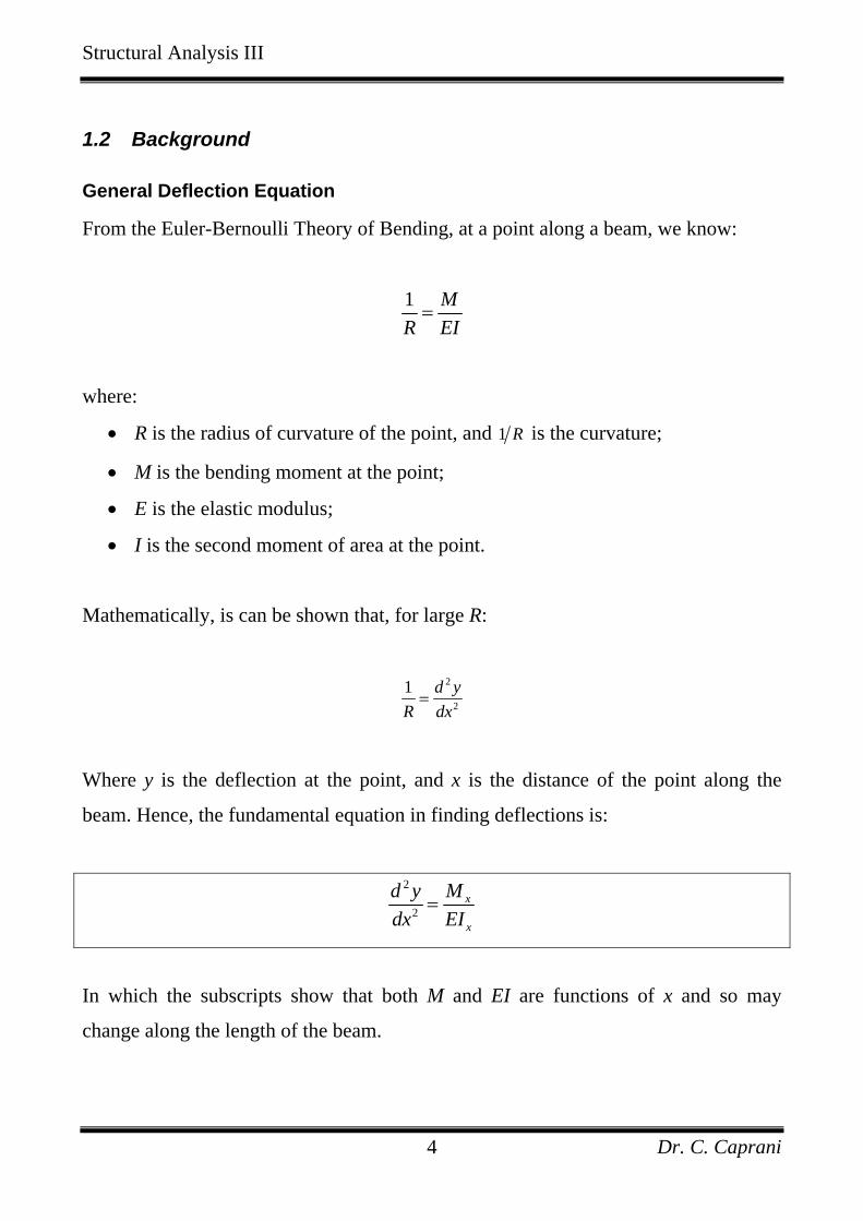
1.2 Background

General Deflection Equation

From the Euler-Bernoulli Theory of Bending, at a point along a beam, we know:

1 MR EI=

where:

• R is the radius of curvature of the point, and 1 R is the curvature;

• M is the bending moment at the point;

• E is the elastic modulus;

• I is the second moment of area at the point.

Mathematically, is can be shown that, for large R:

2

2

1 d yR dx=

Where y is the deflection at the point, and x is the distance of the point along the

beam. Hence, the fundamental equation in finding deflections is:

2

2x

x

d y Mdx EI

=

In which the subscripts show that both M and EI are functions of x and so may

change along the length of the beam.


Dr. C. Caprani 5

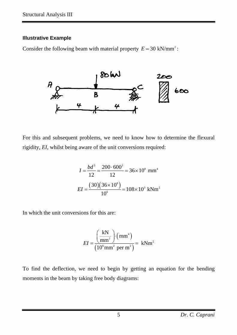
Illustrative Example

Consider the following beam with material property 230 kN/mmE = :

For this and subsequent problems, we need to know how to determine the flexural

rigidity, EI, whilst being aware of the unit conversions required:

3 3

8 4200 600 36 10 mm12 12bdI ⋅

= = = ×

( )( )8

3 26

30 36 10108 10 kNm

10EI

×= = ×

In which the unit conversions for this are:

( )

( )

42

26 2 2

kN mmmm kNm

10 mm per mEI

⎛ ⎞ ⋅⎜ ⎟⎝ ⎠= =

To find the deflection, we need to begin by getting an equation for the bending

moments in the beam by taking free body diagrams:


Dr. C. Caprani 6

For the free-body diagram A to the cut 1 1X X− , 1 1M about 0X X− =∑ gives:

( )( )40 0

40

M x x

M x x

− =

=

For the second cut 2 2M about 0X X− =∑ gives:

( ) ( )( ) ( )

40 80 4 0

40 80 4

M x x x

M x x x

− + − =

= − −


Dr. C. Caprani 7

So the final equation for the bending moment is:

( ) ( )( ) ( )

40 0 4 portion 40 80 4 4 8 portion

x x ABM x

x x x BC⎧ ≤ ≤

= ⎨ − − ≤ ≤⎩

The equations differ by the ( )80 4x− − term, which only comes into play once we are

beyond B where the point load of 80 kN is.

Going back to our basic formula, to find the deflection we use:

( ) ( )2

2 M x M xd y y dx

dx EI EI= ⇒ = ∫∫

But since we have two equations for the bending moment, we will have two different

integrations and four constants of integration.


Dr. C. Caprani 8

Though it is solvable, every extra load would cause two more constants of

integration. Therefore for even ordinary forms of loading, the integrations could be

quite involved.

The solution is to have some means of ‘turning off’ the ( )80 4x− − term when 4x ≤

and turning it on when 4x > . This is what Macaulay’s Method allows us to do. It

recognizes that when 4x ≤ the value in the brackets, ( )4x − , is negative, and when

4x > the value in the brackets is positive. So a Macaulay bracket, [ ]⋅ , is defined to be

zero when the term inside it is negative, and takes its value when the term inside it is

positive:

[ ] 0 44

4 4x

xx x

≤⎧− = ⎨ − >⎩

Another way to think of the Macaulay bracket is:

[ ] ( )4 max 4,0x x− = −

The above is the essence of Macaulay’s Method. The idea of the special brackets is

routed in a strong mathematical background which is required for more advanced

understanding and applications. So we next examine this background, whilst trying

no to loose sight of its essence, explained above.

Note: when implementing a Macaulay analysis in MS Excel or Matlab, it is easier to

use the max function, as above, rather than lots of if statements.


Dr. C. Caprani 9

1.3 Discontinuity Functions

Background

This section looks at the mathematics that lies behind Macaulay’s Method. The

method relies upon special functions which are quite unlike usual mathematical

functions. Whereas usual functions of variables are continuous, these functions have

discontinuities. But it is these discontinuities that make them so useful for our

purpose. However, because of the discontinuities these functions have to be treated

carefully, and we will clearly define how we will use them. There are two types.

Notation

In mathematics, discontinuity functions are usually represented with angled brackets

to distinguish them from other types of brackets:

• Usual ordinary brackets: ( ) [ ] {}⋅ ⋅ ⋅

• Usual discontinuity brackets: ⋅

However (and this is a big one), we will use square brackets to represent our

discontinuity functions. This is because in handwriting they are more easily

distinguishable than the angled brackets which can look similar to numbers.

Therefore, we adopt the following convention here:

• Ordinary functions: ( ) {}⋅ ⋅

• Discontinuity functions: [ ]⋅


Dr. C. Caprani 10

Macaulay Functions

Macaulay functions represent quantities that begin at a point a. Before point a the

function has zero value, after point a the function has a defined value. So, for

example, point a might be the time at which a light was turned on, and the function

then represents the brightness in the room: zero before a and bright after a.

Mathematically:

( ) [ ]( )

0 when

when

where 0,1,2,...

n

nn

x aF x x a

x a x a

n

≤⎧⎪= − = ⎨− >⎪⎩

=

When the exponent 0n = , we have:

( ) [ ]0

0

0 when 1 when

x aF x x a

x a≤⎧

= − = ⎨ >⎩

This is called the step function, because when it is plotted we have:


Dr. C. Caprani 11

For 1n = , we have:

( ) [ ]11

0 when when

x aF x x a

x a x a≤⎧

= − = ⎨ − >⎩

For 2n = , we have:

( ) [ ]( )

2

21

0 when

when

x aF x x a

x a x a

≤⎧⎪= − = ⎨− >⎪⎩

And so on for any value of n.


Dr. C. Caprani 12

Singularity Functions

Singularity functions behave differently to Macaulay functions. They are defined to

be zero everywhere except point a. So in the light switch example the singularity

function could represent the action of switching on the light.

Mathematically:

( ) [ ] 0 when when

where 1, 2, 3,...

n

n

x aF x x a

x an

≠⎧= − = ⎨∞ =⎩

= − − −

The singularity arises since when 1n = − , for example, we have:

( )1

0 when 1when

x aF x

x ax a−

≠⎧⎡ ⎤= = ⎨⎢ ⎥ ∞ =−⎣ ⎦ ⎩

Two singularity functions, very important for us, are:

1. When 1n = − , the function represents a unit force at point a:


Dr. C. Caprani 13

2. When 2n = − , the function represents a unit moment located at point a:

Integration of Discontinuity Functions

These functions can be integrated almost like ordinary functions:

Macaulay functions ( 0n ≥ ):

( ) ( ) [ ] [ ] 1

1

0 0

i.e.1 1

nx xnn

n

x aF xF x x a

n n

+

+ −= − =

+ +∫ ∫

Singularity functions ( 0n < ):

( ) ( ) [ ] [ ] 1

10 0

i.e.x x

n n

n nF x F x x a x a +

+= − = −∫ ∫


Dr. C. Caprani 14

1.4 Modelling of Load Types

Basis

Since our aim is to find a single equation for the bending moments along the beam,

we will use discontinuity functions to represent the loads. However, since we will be

taking moments, we need to know how different load types will relate to the bending

moments. The relationship between moment and load is:

( ) ( ) ( ) ( )and dV x dM x

w x V xdx dx

= =

Thus:

( ) ( )

( ) ( )

2

2

d M xw x

dxM x w x dx

=

= ∫∫

So we will take the double integral of the discontinuity representation of a load to

find its representation in bending moment.


Dr. C. Caprani 15

Moment Load

A moment load of value M, located at point a, is represented by [ ] 2M x a −− and so

appears in the bending moment equation as:

( ) [ ] [ ]2 0M x M x a dx M x a−= − = −∫∫

Point Load

A point load of value P, located at point a, is represented by [ ] 1P x a −− and so

appears in the bending moment equation as:

( ) [ ] [ ]1 1M x P x a dx P x a−= − = −∫∫

Uniformly Distributed Load

A UDL of value w, beginning at point a and carrying on to the end of the beam, is

represented by the step function [ ]0w x a− and so appears in the bending moment

equation as:

( ) [ ] [ ]0 2

2wM x w x a dx x a= − = −∫∫


Dr. C. Caprani 16

Patch Load

If the UDL finishes before the end of the beam – sometimes called a patch load – we

have a difficulty. This is because a Macaulay function ‘turns on’ at point a and never

turns off again. Therefore, to cancel its effect beyond its finish point (point b say), we

turn on a new load that cancels out the original load, giving a net load of zero, as

shown:


Dr. C. Caprani 17

Structurally this is the same as doing the following superposition:

And finally mathematically we represent the patch load that starts at point a and

finishes at point b as:

[ ] [ ]0 0w x a w x b− − −

Giving the resulting bending moment equation as:

( ) [ ] [ ]{ } [ ] [ ]0 0 2 2

2 2w wM x w x a w x b dx x a x b= − − − = − − −∫∫


Dr. C. Caprani 18

1.5 Analysis Procedure

Steps in Analysis

1. Draw a free body diagram of the member and take moments about the cut to

obtain an equation for ( )M x .

2. Equate ( )M x to 2

2

d yEIdx

- this is Equation 1.

3. Integrate Equation 1 to obtain an expression for the rotations along the beam,

dyEIdx

- this is Equation 2, and has rotation constant of integration Cθ .

4. Integrate Equation 2 to obtain an expression for the deflections along the beam,

EIy - this is Equation 3, and has deflection constant of integration Cδ .

5. Us known displacements at support points to calculate the unknown constants

of integration, and any unknown reactions.

6. Substitute the calculated values into the previous equations:

a. Substitute for any unknown reactions;

b. Substitute the value for Cθ into Equation 2, to give Equation 4;

c. Substitute the value for Cδ into Equation 3, giving Equation 5.

7. Solve for required displacements by substituting the location into Equation 4 or

5 as appropriate.

Note that the constant of integration notation reflects the following:

• Cθ is the rotation where 0x = , i.e. the start of the beam;

• Cδ is the deflection where 0x = .

The constants of integration will always be in units of kN and m since we will keep

our loads and distances in these units. Thus our final deflections will be in units of m,

and our rotations in units of rads.


Dr. C. Caprani 19

Finding the Maximum Deflection

A usual problem is to find the maximum deflection. Given any curve ( )y f x= , we

know from calculus that y reaches a maximum at the location where 0dydx

= . This is

no different in our case where y is now deflection and dydx

is the rotation. Therefore:

A local maximum displacement occurs at a point of zero rotation

The term local maximum indicates that there may be a few points on the deflected

shape where there is zero rotation, or local maximum deflections. The overall biggest

deflection will be the biggest of these local maxima. For example:

So in this beam we have 0θ = at two locations, giving two local maximum

deflections, 1,maxy and 2,maxy . The overall largest deflection is ( )max 1,max 2,maxmax ,y y y= .

Lastly, to find the location of the maximum deflection we need to find where 0θ = .

Thus we need to solve the problem’s Equation 4 to find an x that gives 0θ = .

Sometimes this can be done algebraically, but often it is done using trial and error.

Once the x is found that gives 0θ = , we know that this is also a local maximum

deflection and so use this x in Equation 5 to find the local maximum deflection.


Dr. C. Caprani 20

Sign Convention

In Macaulay’s Method, we will assume there to be tension on the bottom of the

member by drawing our ( )M x arrow coming from the bottom of the member. By

doing this, we orient the x-y axis system as normal: positive y upwards; positive x to

the right; anti-clockwise rotations are positive – all as shown below. We do this even

(e.g. a cantilever) where it is apparent that tension is on top of the beam. In this way,

we know that downward deflections will always be algebraically negative.

When it comes to frame members at an angle, we just imagine the above diagrams

rotated to the angle of the member.


Dr. C. Caprani 21

2. Determinate Beams

2.1 Example 1 – Point Load

Here we take the beam looked at previously and calculate the rotations at the

supports, show the maximum deflection is at midspan, and calculate the maximum

deflection:

Step 1

The appropriate free-body diagram is:

Note that in this diagram we have taken the cut so that all loading is accounted for.

Taking moments about the cut, we have:


Dr. C. Caprani 22

( ) [ ]40 80 4 0M x x x− + − =

In which the Macaulay brackets have been used to indicate that when 4x ≤ the term

involving the 80 kN point load should become zero. Hence:

( ) [ ]40 80 4M x x x= − −

Step 2

Thus we write:

( ) [ ]2

2 40 80 4d yM x EI x xdx

= = − − Equation 1

Step 3

Integrate Equation 1 to get:

[ ]2240 80 42 2

dyEI x x Cdx θ= − − + Equation 2

Step 4


[ ]3340 80 46 6

EIy x x C x Cθ δ= − − + + Equation 3

Notice that we haven’t divided in by the denominators. This makes it easier to check

for errors since, for example, we can follow the 40 kN reaction at A all the way

through the calculation.


Dr. C. Caprani 23

Step 5

To determine the constants of integration we use the known displacements at the

supports. That is:

• Support A: located at 0x = , deflection is zero, i.e. 0y = ;

• Support C: located at 8x = , deflection is zero, i.e. 0y = .

So, using Equation 3, for the first boundary condition, 0y = at 0x = gives:

( ) ( ) [ ] ( )3340 800 0 0 4 06 6

EI C Cθ δ= − − + +

Impose the Macaulay bracket to get:

( ) ( ) [ ]3340 800 0 0 46 6

EI = − − ( )0

0 0 0 0

C C

C

θ δ

δ

+ +

= − + +

Therefore:

0Cδ =

Again using Equation 3 for the second boundary condition of 0y = at 8x = gives:

( ) ( ) [ ] ( )3340 800 8 8 4 8 06 6

EI Cθ= − − + +

Since the term in the Macaulay brackets is positive, we keep its value. Note also that

we have used the fact that we know 0Cδ = . Thus:


Dr. C. Caprani 24

20480 51200 86 6

48 15360320

C

CC

θ

θ

θ

= − +

= −= −

Which is in units of kN and m, as discussed previously.

Step 6

Now with the constants known, we re-write Equations 2 & 3 to get Equations 4 & 5:

[ ]2240 80 4 3202 2

dyEI x xdx

= − − − Equation 4

[ ]3340 80 4 3206 6

EIy x x x= − − − Equation 5

With Equations 4 & 5 found, we can now calculate any deformation of interest.

Rotation at A

We are interested in A

dydx

θ ≡ at 0x = . Thus, using Equation 4:

( ) [ ]2240 800 0 42 2AEIθ = − − 320

320320

A

A

EI

EI

θ

θ

−

= −−

=

From before we have 3 2108 10 kNmEI = × , hence:


Dr. C. Caprani 25

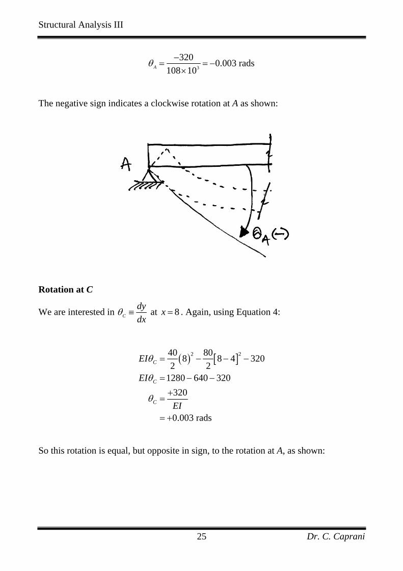
3

320 0.003 rads108 10Aθ−

= = −×

The negative sign indicates a clockwise rotation at A as shown:

Rotation at C

We are interested in C

dydx

θ ≡ at 8x = . Again, using Equation 4:

( ) [ ]2240 808 8 4 3202 2

1280 640 320320

0.003 rads

C

C

C

EI

EI

EI

θ

θ

θ

= − − −

= − −

+=

= +

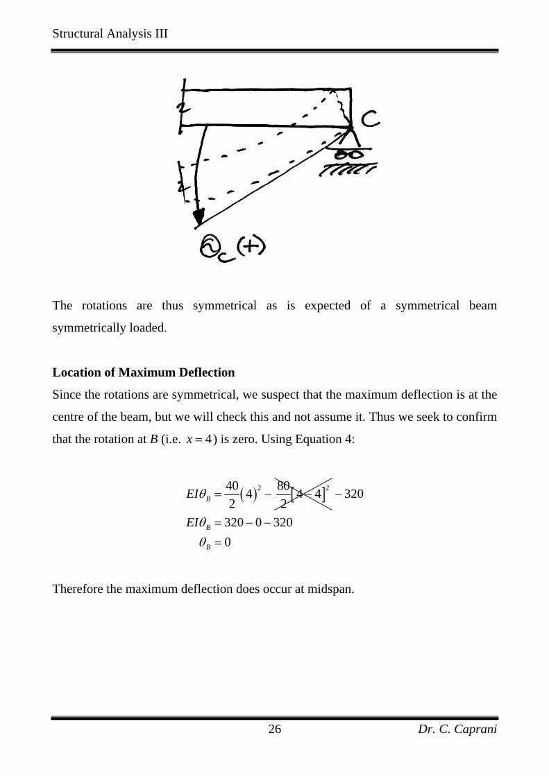
So this rotation is equal, but opposite in sign, to the rotation at A, as shown:


Dr. C. Caprani 26

The rotations are thus symmetrical as is expected of a symmetrical beam

symmetrically loaded.

Location of Maximum Deflection

Since the rotations are symmetrical, we suspect that the maximum deflection is at the

centre of the beam, but we will check this and not assume it. Thus we seek to confirm

that the rotation at B (i.e. 4x = ) is zero. Using Equation 4:

( ) [ ]2240 804 4 42 2BEIθ = − − 320

320 0 3200

B

B

EIθθ

−

= − −=

Therefore the maximum deflection does occur at midspan.


Dr. C. Caprani 27

Maximum Deflection

Substituting 4x = , the location of the zero rotation, into Equation 5:

( ) [ ]3340 804 4 46 6BEIδ = − − ( )320 4

2560 0 12806853.33

B

B

EI

EI

δ

δ

−

= − −

−=

In which we have once again used the Macaulay bracket. Thus:

33

853.33 7.9 10 m108 10

7.9 mm

Bδ−−

= = − ××

= −

Since the deflection is negative we know it to be downward as expected.

In summary then, the final displacements are:


Dr. C. Caprani 28

2.2 Example 2 – Patch Load

In this example we take the same beam as before with the same load as before, except

this time the 80 kN load will be spread over 4 m to give a UDL of 20 kN/m applied to

the centre of the beam as shown:

Step 1

Since we are dealing with a patch load we must extend the applied load beyond D

(due to the limitations of a Macaulay bracket) and put an upwards load from D

onwards to cancel the effect of the extra load. Hence the free-body diagram is:


Dr. C. Caprani 29

Again we have taken the cut far enough to the right that all loading is accounted for.


( ) [ ] [ ]2 220 2040 2 6 02 2

M x x x x− + − − − =

Again the Macaulay brackets have been used to indicate when terms should become

zero. Hence:

( ) [ ] [ ]2 220 2040 2 62 2

M x x x x= − − + −

Step 2

Thus we write:

( ) [ ] [ ]2

2 22

20 2040 2 62 2

d yM x EI x x xdx

= = − − + − Equation 1

Step 3


[ ] [ ]3 3240 20 202 62 6 6

dyEI x x x Cdx θ= − − + − + Equation 2

Step 4


[ ] [ ]4 4340 20 202 66 24 24

EIy x x x C x Cθ δ= − − + − + + Equation 3


Dr. C. Caprani 30

As before, notice that we haven’t divided in by the denominators.

Step 5

The boundary conditions are:

• Support A: 0y = at 0x = ;

• Support B: 0y = at 8x = .

So for the first boundary condition:

( ) ( ) [ ]4340 200 0 0 26 24

EI = − − [ ]420 0 624

+ − ( )0C Cθ δ+ +

0Cδ =

For the second boundary condition:

( ) ( ) ( ) ( )3 4 440 20 200 8 6 2 86 24 24293.33

EI C

C

θ

θ

= − + +

= −

Step 6

Insert constants into Equations 2 & 3:

[ ] [ ]3 3240 20 202 6 293.332 6 6

dyEI x x xdx

= − − + − − Equation 4

[ ] [ ]4 4340 20 202 6 293.336 24 24

EIy x x x x= − − + − − Equation 5


Dr. C. Caprani 31

To compare the effect of smearing the 80 kN load over 4 m rather than having it

concentrated at midspan, we calculate the midspan deflection:

( ) ( ) [ ]43 4max

40 20 204 2 4 66 24 24

EIδ = − + − ( )293.33 4

760

−

= −

Therefore:

max 3

max

760 760 0.00704 m108 20

7.04 mmEI

δ

δ

− −= = = −

×= −

This is therefore a downward deflection as expected. Comparing it to the 7.9 mm

deflection for the 80 kN point load, we see that smearing the load has reduced

deflection, as may be expected.

Problem:

• Verify that the maximum deflection occurs at the centre of the beam;

• Calculate the end rotations.


Dr. C. Caprani 32

2.3 Example 3 – Moment Load

For this example we take the same beam again, except this time it is loaded by a

moment load at midspan, as shown:

Before beginning Macaulay’s Method, we need to calculate the reactions:

Step 1

The free-body diagram is:


Dr. C. Caprani 33


( ) [ ]010 80 4 0M x x x+ − − =

Notice a special point here. We have used our knowledge of the singularity function

representation of a moment load to essentially locate the moment load at 4x = in the

equations above. Refer back to page 15 to see why this is done. Continuing:

( ) [ ]010 80 4M x x x= − + −

Step 2

( ) [ ]2

02 10 80 4d yM x EI x x

dx= = − + − Equation 1

Step 3

[ ]1210 80 42

dyEI x x Cdx θ= − + − + Equation 2

Step 4

[ ]2310 80 46 2

EIy x x C x Cθ δ= − + − + + Equation 3

Step 5

We know 0y = at 0x = , thus:

( ) ( ) [ ]2310 800 0 0 46 2

EI = − + − ( )0

0

C C

C

θ δ

δ

+ +

=


Dr. C. Caprani 34

0y = at 8x = , thus:

( ) ( ) ( )3 210 800 8 4 8

6 2803

EI C

C

θ

θ

= − + +

= +

Step 6

[ ]1210 8080 42 3

dyEI x xdx

= − + − + Equation 4

[ ]2310 80 8046 2 3

EIy x x x= − + − + Equation 5

So for the deflection at C:

( ) [ ]2310 804 4 46 2CEIδ = − + − ( )80 4

30CEIδ

+

=

Problem:

• Verify that the rotation at A and B are equal in magnitude and sense;

• Find the location and value of the maximum deflection.


Dr. C. Caprani 35

2.4 Example 4 – Beam with Overhangs and Multiple Loads

For the following beam, determine the maximum deflection, taking 3 220 10 kNmEI = × :

Before beginning Macaulay’s Method, we need to calculate the reactions:

Taking moments about B:

( ) ( ) 240 2 10 2 2 8 40 0

2

2.5 kN i.e.

E

E

V

V

⎧ ⎫⎛ ⎞− ⋅ + ⋅ ⋅ + − + =⎨ ⎬⎜ ⎟⎝ ⎠⎩ ⎭

= + ↑


Dr. C. Caprani 36

Summing vertical forces:

( )2.5 40 2 10 0

57.5 kN, i.e. B

B

V

V

+ − − ⋅ =

= + ↑

With the reactions calculated, we begin by drawing the free body diagram for

Macaulay’s Method:

Note the following points:

• The patch load has been extended all the way to the end of the beam and a

cancelling load has been applied from D onwards;

• The cut has been taken so that all forces applied to the beam are to the left of

the cut. Though the 40 kNm moment is to the right of the cut, and so not in the

diagram, its effect is accounted for in the reactions which are included.


Dr. C. Caprani 37

Taking moments about the cut:

( ) [ ] [ ] [ ] [ ]2 210 1040 57.5 2 4 6 2.5 10 02 2

M x x x x x x+ − − + − − − − − =

So we have Equation 1:

( ) [ ] [ ] [ ] [ ]2

2 2

2

10 1040 57.5 2 4 6 2.5 102 2

d yM x EI x x x x xdx

= = − + − − − + − + −

Integrate for Equation 2:

[ ] [ ] [ ] [ ]2 3 3 2240 57.5 10 10 2.52 4 6 102 2 6 6 2

dyEI x x x x x Cdx θ= − + − − − + − + − +

And again for Equation 3:

[ ] [ ] [ ] [ ]3 4 4 3340 57.5 10 10 2.52 4 6 106 6 24 24 6

EIy x x x x x C x Cθ δ= − + − − − + − + − + +

Using the boundary condition at support B where 0y = at 2x = :

( ) ( ) [ ]3340 57.50 2 2 26 6

EI = − + − [ ]410 2 424

− − [ ]410 2 624

+ − [ ]32.5 2 106

+ − 2C Cθ δ+ +

Thus:

16023

C Cθ δ+ = (a)


Dr. C. Caprani 38

The second boundary condition is 0y = at 10x = :

( ) ( ) ( ) ( ) ( ) [ ]33 3 4 440 57.5 10 10 2.50 10 8 6 4 10 106 6 24 24 6

EI = − + − + + − 10C Cθ δ+ +

Hence:

6580103

C Cθ δ+ = (b)

Subtracting (a) from (b) gives:

64208 267.53

C Cθ θ= ⇒ = +

And:

( ) 1602 267.5 481.73

C Cδ δ+ = ⇒ = −

Thus we have Equation 4:

[ ] [ ] [ ] [ ]2 3 3 2240 57.5 10 10 2.52 4 6 10 267.52 2 6 6 2

dyEI x x x x xdx

= − + − − − + − + − +

And Equation 5:

[ ] [ ] [ ] [ ]3 4 4 3340 57.5 10 10 2.52 4 6 10 267.5 481.76 6 24 24 6

EIy x x x x x x= − + − − − + − + − + −


Dr. C. Caprani 39

Since we are interested in finding the maximum deflection, we solve for the shear,

bending moment, and deflected shape diagrams, in order to better visualize the

beam’s behaviour:

So examining the above, the overall maximum deflection will be the biggest of:

• Aδ - the deflection of the tip of the cantilever at A – found from Equation 5

using 0x = ;

• Fδ - the deflection of the tip of the cantilever at F – again got from Equation 5

using 11x = ;

• max BEδ - the largest upward deflection somewhere between the supports – its

location is found solving Equation 4 to find the x where 0θ = , and then

substituting this value into Equation 5.


Dr. C. Caprani 40

Maximum Deflection Between B and E

Since Equation 4 cannot be solved algebraically for x, we will use trial and error.

Initially choose the midspan, where 6x = :

( ) ( ) ( ) [ ]32 2 3

6

40 57.5 10 106 4 2 6 62 2 6 6x

dyEIdx =

= − + − + − [ ]22.5 6 102

+ − 267.5

5.83

+

= −

Try reducing x to get closer to zero, say 5.8x = :

( ) ( ) ( ) [ ]32 2 3

5.8

40 57.5 10 105.8 3.8 1.8 5.8 62 2 6 6x

dyEIdx =

= − + − + − [ ]22.5 5.8 102

+ − 267.5

0.13

+

= +

Since the sign of the rotation has changed, zero rotation occurs between 5.8x = and

6x = . But it is apparent that zero rotation occurs close to 5.8x = . Therefore, we will

use 5.8x = since it is close enough (you can check this by linearly interpolating

between the values).

So, using 5.8x = , from Equation 5 we have:

( ) ( ) ( ) [ ]43 3 4

max

40 57.5 10 105.8 3.8 1.8 5.8 66 6 24 24

EI BEδ = − + − + − [ ]32.5 5.8 106

+ −

( )max

267.5 5.8 481.7

290.5EI BEδ

+ −

= +

Thus we have:


Dr. C. Caprani 41

max 3

290.5 290.5 0.01453 m20 10

14.53 mm

BEEI

δ = + = + = +×

= +

Since the result is positive it represents an upward deflection.

Deflection at A

Substituting 0x = into Equation 5 gives:

( ) [ ]3340 57.50 0 26 6AEIδ = − + − [ ]410 0 4

24− − [ ]410 0 6

24+ − [ ]32.5 0 10

6+ −

( )267.5 0 481.7481.7AEIδ

+ −

= −

Hence

3

481.7 481.7 0.02409 m20 10

24.09 mm

A EIδ = − = − = −

×= −

Since the result is negative the deflection is downward. Note also that the deflection

at A is the same as the deflection constant of integration, Cδ . This is as mentioned

previously on page 18.

Deflection at F

Substituting 11x = into Equation 5 gives:

( ) ( ) ( ) ( ) ( )

( )

3 3 4 4 340 57.5 10 10 2.511 9 7 5 16 6 24 24 6

267.5 11 481.7165.9

F

F

EI

EI

δ

δ

= − + − + +

+ −

= −


Dr. C. Caprani 42

Giving:

3

165.9 165.9 0.00830 m20 10

8.30 mm

F EIδ = − = − = −

×= −

Again the negative result indicates the deflection is downward.

Maximum Overall Deflection

The largest deviation from zero anywhere in the beam is thus at A, and so the

maximum deflection is 24.09 mm, as shown:


Dr. C. Caprani 43

2.5 Example 5 – Beam with Hinge

For the following prismatic beam, find the following:

• The rotations at the hinge;

• The deflection of the hinge;

• The maximum deflection in span BE.

Before beginning the deflection calculations, calculate the reactions:

This beam is made of two members: AB and BE. The Euler-Bernoulli deflection

equation only applies to individual members, and does not apply to the full beam AB

since there is a discontinuity at the hinge, B. The discontinuity occurs in the rotations

at B, since the ends of members AB and BE have different slopes as they connect to


Dr. C. Caprani 44

the hinge. However, there is also compatibility of displacement at the hinge in that

the deflection of members AB and BE must be the same at B – there is only one

vertical deflection at the hinge. From the previous examples we know that each

member will have two constant of integration, and thus, for this problem, there will

be four constants in total. However, we have the following knowns:

• Deflection at A is zero;

• Rotation at A is zero;

• Deflection at D is zero;

• Deflection at B is the same for members AB and BE;

Thus we can solve for the four constants and the problem as a whole. To proceed we

consider each span separately initially.

Span AB

The free-body diagram for the deflection equation is:

Note that even though it is apparent that there will be tension on the top of the

cantilever, we have retained our sign convention by taking ( )M x as tension on the

bottom. Taking moments about the cut:

( ) 220360 130 02

M x x x+ − + =


Dr. C. Caprani 45

Hence, the calculations proceed as:

( )2

22

20130 3602

d yM x EI x xdx

= = − − Equation (AB)1

2 3130 203602 6

dyEI x x x Cdx θ= − − + Equation (AB)2

3 2 4130 360 206 2 24

EIy x x x C x Cθ δ= − − + + Equation (AB)3

At 0x = , 0y = :

( ) ( ) ( ) ( ) ( )3 2 4130 360 200 0 0 0 0 06 2 24

EI C C Cθ δ δ= − − + + ⇒ =

At 0x = , 0A

dydx

θ = = :

( ) ( ) ( ) ( )2 3130 200 0 360 0 0 02 6

EI C Cθ θ= − − + ⇒ =

Thus the final equations are:

2 3130 203602 6

dyEI x x xdx

= − − Equation (AB)4

3 2 4130 360 206 2 24

EIy x x x= − − Equation (AB)5


Dr. C. Caprani 46

Span BE

The relevant free-body diagram is:

Thus:

( ) [ ] [ ]100 2 50 50 4 0M x x x x+ − − − − =

( ) [ ] [ ]2

250 50 4 100 2d yM x EI x x x

dx= = + − − − Equation (BE)1

[ ] [ ]2 2250 50 1004 22 2 2

dyEI x x x Cdx θ= + − − − + Equation (BE)2

[ ] [ ]3 3350 50 1004 26 6 6

EIy x x x C x Cθ δ= + − − − + + Equation (BE)3

At B, we can calculate the deflection from member AB’s Equation (AB)5. Thus:


Dr. C. Caprani 47

( ) ( ) ( )3 2 4130 360 204 4 4

6 2 241707

B

B

EI

EI

δ

δ

= − −

−=

This is a downward deflection and must also be the deflection at B for member BE, so

from Equation (BE)3:

( ) [ ]331707 50 500 0 46 6

EIEI

−⎛ ⎞ = + −⎜ ⎟⎝ ⎠

[ ]3100 0 26

− − ( )0

1707

C C

C

θ δ

δ

+ +

= −

Notice that again we find the deflection constant of integration to be the value of

deflection at the start of the member.

Representing the deflection at support D, we know that at 4x = , 0y = for member

BE. Thus using Equation (BE)3 again:

( ) ( ) [ ]3350 500 4 4 46 6

EI = + − ( ) ( )3100 2 4 17076

327

C

C

θ

θ

− + −

= +

Giving Equation (BE)4 and Equation (BE)5 respectively as:

[ ] [ ]2 2250 50 1004 2 3272 2 2

dyEI x x xdx

= + − − − +

[ ] [ ]3 3350 50 1004 2 327 17076 6 6

EIy x x x x= + − − − + −


Dr. C. Caprani 48

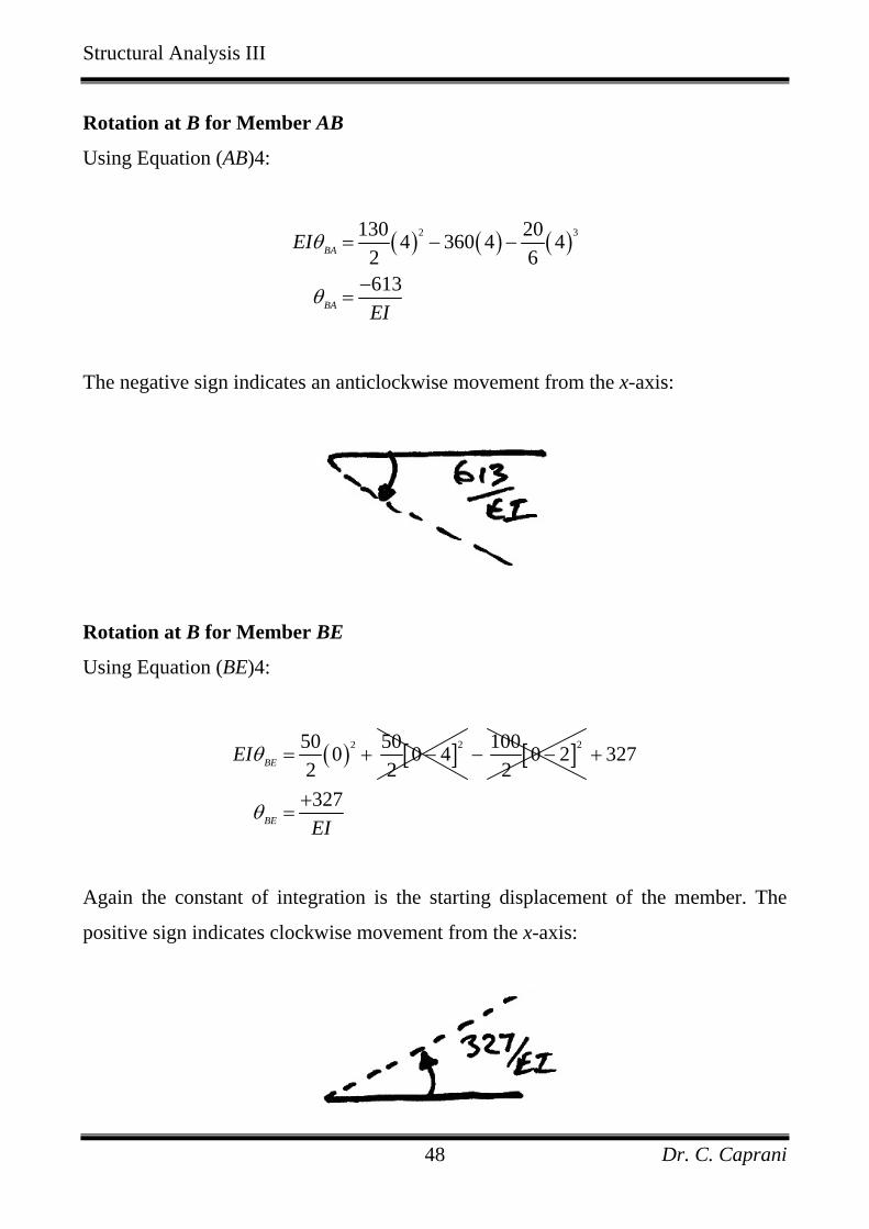
Rotation at B for Member AB

Using Equation (AB)4:

( ) ( ) ( )2 3130 204 360 4 4

2 6613

BA

BA

EI

EI

θ

θ

= − −

−=

The negative sign indicates an anticlockwise movement from the x-axis:

Rotation at B for Member BE

Using Equation (BE)4:

( ) [ ]2250 500 0 4

2 2BEEIθ = + − [ ]2100 0 22

− − 327

327BE EI

θ

+

+=

Again the constant of integration is the starting displacement of the member. The

positive sign indicates clockwise movement from the x-axis:


Dr. C. Caprani 49

Thus at B the deflected shape is:

Deflection at B

Calculated previously to be 1707B EIδ = − .

Maximum Deflection in Member BE

There are three possibilities:

• The maximum deflection is at B – already known;

• The maximum deflection is at E – to be found;

• The maximum deflection is between B and D – to be found.

The deflection at E is got from Equation (BE)5:

( ) ( ) ( ) ( )3 3 350 50 1006 2 4 327 6 1707

6 6 61055

E

E

EI

EI

δ

δ

= + − + −

+=

And this is an upwards displacement which is smaller than that of the movement at B.

To find the maximum deflection between B and D, we must identify the position of

zero rotation. Since at the start of the member (i.e. at B) we know the rotation is

positive ( 327BE EIθ = + ), zero rotation can only occur if the rotation at the other end


Dr. C. Caprani 50

of the member (rotation at E) is negative. However, we know the rotation at E is the

same as that at D since DE is straight because there is no bending in it. Hence we find

the rotation at D to see if it is negative, from Equation (BE)4:

( ) [ ]2250 504 4 4

2 2DEIθ = + − ( )2100 2 3272

527D EI

θ

− +

+=

Since this is positive, there is no point at which zero rotation occurs between B and D

and thus there is no position of maximum deflection. Therefore the largest deflections

occur at the ends of the member, and are as calculated previously:

As a mathematical check on our structural reasoning above, we attempt to solve

Equation (BE)4 for x when 0dydx

= :

( ) [ ] [ ]2 22

2 2 2

50 50 1000 4 2 3272 2 2

50 50 1000 8 16 4 4 3272 2 2

EI x x x

x x x x x

= + − − − +

= + − + − − + +⎡ ⎤ ⎡ ⎤⎣ ⎦ ⎣ ⎦


Dr. C. Caprani 51

Collecting terms, we have:

( ) ( )

2

2

50 50 100 400 400 800 4000 3272 2 2 2 2 2 2

0 0 0 5270 527

x x

x x

−⎛ ⎞ ⎛ ⎞ ⎛ ⎞= + − + + + − +⎜ ⎟ ⎜ ⎟ ⎜ ⎟⎝ ⎠ ⎝ ⎠ ⎝ ⎠

= + +

=

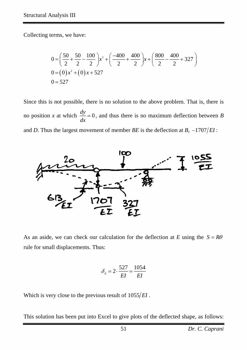
Since this is not possible, there is no solution to the above problem. That is, there is

no position x at which 0dydx

= , and thus there is no maximum deflection between B

and D. Thus the largest movement of member BE is the deflection at B, 1707 EI− :

As an aside, we can check our calculation for the deflection at E using the S Rθ=

rule for small displacements. Thus:

527 10542E EI EIδ = ⋅ =

Which is very close to the previous result of 1055 EI .

This solution has been put into Excel to give plots of the deflected shape, as follows:


Dr. C. Caprani 52

X global X for AB X for BE dy/dx AB y AB dy/dx BE y BE0.00 0.00 -4.00 0.0 0.0 727.0 -3548.30.25 0.25 -3.75 -86.0 -10.9 678.6 -3372.70.50 0.50 -3.50 -164.2 -42.3 633.3 -3208.80.75 0.75 -3.25 -234.8 -92.4 591.1 -3055.81.00 1.00 -3.00 -298.3 -159.2 552.0 -2913.01.25 1.25 -2.75 -354.9 -241.0 516.1 -2779.61.50 1.50 -2.50 -405.0 -336.1 483.3 -2654.71.75 1.75 -2.25 -448.8 -442.9 453.6 -2537.72.00 2.00 -2.00 -486.7 -560.0 427.0 -2427.72.25 2.25 -1.75 -518.9 -685.8 403.6 -2323.92.50 2.50 -1.50 -545.8 -819.0 383.3 -2225.62.75 2.75 -1.25 -567.8 -958.3 366.1 -2132.03.00 3.00 -1.00 -585.0 -1102.5 352.0 -2042.33.25 3.25 -0.75 -597.9 -1250.4 341.1 -1955.83.50 3.50 -0.50 -606.7 -1401.1 333.3 -1871.53.75 3.75 -0.25 -611.7 -1553.5 328.6 -1788.94.00 4.00 0.00 -613.3 -1706.7 327.0 -1707.04.25 0.25 328.6 -1625.14.50 0.50 333.3 -1542.54.75 0.75 341.1 -1458.25.00 1.00 352.0 -1371.75.25 1.25 366.1 -1282.05.50 1.50 383.3 -1188.45.75 1.75 403.6 -1090.16.00 2.00 427.0 -986.36.25 2.25 450.4 -876.66.50 2.50 470.8 -761.46.75 2.75 487.9 -641.57.00 3.00 502.0 -517.77.25 3.25 512.9 -390.77.50 3.50 520.8 -261.57.75 3.75 525.4 -130.68.00 4.00 527.0 1.08.25 4.25 527.0 132.88.50 4.50 527.0 264.58.75 4.75 527.0 396.39.00 5.00 527.0 528.09.25 5.25 527.0 659.8 dy/dx AB = 130*x^2/2-360*x-20*x^3/69.50 5.50 527.0 791.5 y AB = 130*x^3/6-360*x^2/2-20*x^4/249.75 5.75 527.0 923.3 dy/dx BE = 50*x^2/2+50*MAX(x-4,0)^2/2-100*MAX(x-2,0)^2/2+32710.00 6.00 527.0 1055.0 y BE = 50*x^3/6+50*MAX(x-4,0)^3/6-100*MAX(x-2,0)^3/6+327*x-1707

Macaulay's Method - Determinate Beam with Hinge

Equation used in the Cells

-800.0

-600.0

-400.0

-200.0

0.0

200.0

400.0

600.0

800.0

0.00 2.00 4.00 6.00 8.00 10.00

Distance Along Beam (m)

Rot

atio

n - (

dy/d

x)/E

I

dy/dx for AB

dy/dx for BE (4<x<10)

dy/dx for BE (x<4)

-4000.0

-3000.0

-2000.0

-1000.0

0.0

1000.0

2000.0

0.00 2.00 4.00 6.00 8.00 10.00

Distance Along Beam (m)D

efle

ctio

n -y

/EI

y for ABy for BE (4<x<10)y for BE (x<4)


Dr. C. Caprani 53

2.6 Problems

1. (DT004/3 A’03) Determine the rotation and the deflection at C for the

following beam. Take 2200 kN/mmE = and 8 48 10 mmI = × . (Ans. 4.46 mm,

0.0775 rads).

40 kN

A B C

15 kN/m

6 m 2 m

2. (DT004/3 S’04) Determine the rotation at A, the rotation at B, and the

deflection at C, for the following beam. Take 2200 kN/mmE = and 8 48 10 mmI = × . (Ans. 365A EIθ = ; 361.67B EIθ = ; 900c EIδ = ).

2 m

50 kN

A BC

20 kN/m

4 m 2 m

3. (DT004/3 A’04) Determine the deflection at C, for the following beam. Check

your answer using 4 35 384 48C wL EI PL EIδ = + . Take 2200 kN/mmE = and 8 48 10 mmI = × . The symbols w, L and P have their usual meanings. (Ans. 5.34

mm).

50 kN

A BC

12 kN/m

6 m


Dr. C. Caprani 54

4. (DT004/3 S’05) Determine the deflection at B and D for the following beam.

Take 2200 kN/mmE = and 8 48 10 mmI = × . (Ans. 2.95 mm ↑ , 15.1 mm ↓ ).

ACB

12 kN/m

3 m

50 kN

3 m 3 m

D

5. (DT004/3 A’05) Verify that the rotation at A is smaller than that at B for the

following beam. Take 2200 kN/mmE = and 8 48 10 mmI = × . (Ans.

186.67A EIθ = − ; 240B EIθ = − ; 533.35C EIδ = − ).

A BC

20 kN/m

4 m 4 m

6. (DT004/3 S’06) Determine the location of the maximum deflection between A

and B, accurate to the nearest 0.01 m and find the value of the maximum

deflection between A and B, for the following beam. Take 2200 kN/mmE =

and 8 48 10 mmI = × . (Ans. 2.35 m; -2.55 mm)

AB

15 kN/m

3 m 3 mC

80 kNm

2 m


Dr. C. Caprani 55

7. (DT004/3 A’06) Determine the location of the maximum deflection between A

and B, accurate to the nearest 0.01 m and find the value of the maximum

deflection between A and B, for the following beam. Take 2200 kN/mmE =

and 8 48 10 mmI = × . (Ans. 2.40 m; 80 EI ).

40 kN

A B C

15 kN/m

6 m 2 m

8. (DT004/3 S2R’07) Determine the rotation at A, the rotation at B, and the

deflection at C, for the following beam. Check your answer using 4 35 384 48C wL EI PL EIδ = + . Take 2200 kN/mmE = and 8 48 10 mmI = × .

The symbols w, L and P have their usual meanings. (Ans. -360/EI, +360/EI, -

697.5/EI)

80 kN

A BC

20 kN/m

6 m


Dr. C. Caprani 56

3. Indeterminate Beams

3.1 Basis

In solving statically determinate structures, we have seen that application of

Macaulay’s Method gives two unknowns:

1. Rotation constant of integration;

2. Deflection constant of integration.

These unknowns are found using the known geometrically constraints (or boundary

conditions) of the member. For example, at a pin or roller support we know the

deflection is zero, whilst at a fixed support we know that both deflection and rotation

are zero. Form what we have seen we can conclude that in any stable statically

determinate structure there will always be enough geometrical constraints to find the

two knowns – if there isn’t, the structure simply is not stable, and is a mechanism.

Considering indeterminate structures, we will again have the same two unknown

constants of integration, in addition to the extra unknown support reactions.

However, for each extra support introduced, we have an associated geometric

constraint, or known displacement. Therefore, we will always have enough

information to solve any structure. It simply falls to us to express our equations in

terms of our unknowns (constants of integration and redundant reactions) and apply

our known displacements to solve for these unknowns, thus solving the structure as a

whole.

This is best explained by example, but keep in mind the general approach we are

using.


Dr. C. Caprani 57

3.2 Example 6 – Propped Cantilever with Overhang

Determine the maximum deflection for the following prismatic beam, and solve for

the bending moment, shear force and deflected shape diagrams.

Before starting the problem, consider the qualitative behaviour of the structure so that

we have an idea of the reactions’ directions and the deflected shape:

Since this is a 1˚ indeterminate structure we must choose a redundant and the use the

principle of superposition:


Dr. C. Caprani 58

Next, we express all other reactions in terms of the redundant, and draw the free-body

diagram for Macaulay’s Method:

Proceeding as usual, we take moments about the cut, being careful to properly locate

the moment reaction at A using the correct discontinuity function format:

( ) ( )[ ] ( ) [ ]06 900 100 6 0M x R x R x R x− − − − − − =

Since x will always be positive we can remove the Macaulay brackets for the moment

reaction at A, and we then have:

( ) ( ) ( ) [ ]2

02

6 900 100 6d yM x EI R x R x R xdx

= = − + − + − Equation 1

From which:

( ) ( ) [ ]221006 900 6

2 2Rdy REI R x x x C

dx θ

−= − + + − + Equation 2

And:


Dr. C. Caprani 59

( ) ( ) [ ]32 36 900 1006

2 6 6R R REIy x x x C x Cθ δ

− −= + + − + + Equation 3

Thus we have three unknowns to solve for, and we have three knowns we can use:

1. no deflection at A – fixed support;

2. no rotation at A – fixed support;

3. no deflection at B – roller support.

As can be seen the added redundant support both provides an extra unknown

reaction, as well as an extra known geometric condition.

Applying the first boundary condition, we know that at 0x = , 0y = :

( ) ( ) ( ) ( ) ( ) [ ]32 36 900 1000 0 0 0 6

2 6 6R R REI− −

= + + − ( )0

0

C C

C

θ δ

δ

+ +

=

Applying the second boundary condition, at 0x = , 0dydx

= :

( ) ( )( ) ( ) ( ) [ ]221000 6 900 0 0 0 6

2 2R REI R

−= − + + −

0

C

C

θ

θ

+

=

Applying the final boundary condition, at 6x = , 0y = :

( ) ( ) ( ) ( ) ( ) [ ]32 36 900 1000 6 6 6 6

2 6 6R R REI− −

= + + −

( ) ( )0 108 16200 3600 36R R= − + −


Dr. C. Caprani 60

Thus we have an equation in R and we solve as:

0 72 12600175 kN

RR= −

= ↑

The positive answer means the direction we assumed initially was correct. We can

now solve for the other reactions:

( )6 900 6 175 900 150 kNm

100 100 175 75 kN i.e. A

A

M R

V R

= − = − = +

= − = − = − ↓

We now write Equations 4 and 5:

[ ]2275 175150 62 2

dyEI x x xdx

−= + + −

[ ]32 3150 75 175 62 6 6

EIy x x x−= + + −

Finally to find the maximum deflection, we see from the qualitative behaviour of the

structure that it will either be at the tip of the overhang, C, or between A and B. For

the deflection at C, where 9x = , we have, from Equation 5:

( ) ( ) ( )2 3 3150 75 1759 9 3

2 6 62250

C

C

EI

EI

δ

δ

−= + +

−=

This is downwards as expected. To find the local maximum deflection in Span AB,

we solve for its location using Equation 4:


Dr. C. Caprani 61

( ) [ ]2275 1750 150 62 2

EI x x x−= + + − since 6

0 150 37.5150 4 m37.5

x

x

x

≤

= −

= =

Therefore from Equation 5:

( ) ( ) [ ]32 3

max

150 75 1754 4 4 62 6 6

EI ABδ −= + + −

max

400ABEI

δ +=

The positive result indicates an upward displacement, as expected. Therefore the

maximum deflection is at C, and the overall solution is:


Dr. C. Caprani 62

3.3 Example 7 – Indeterminate Beam with Hinge

For the following prismatic beam, find the rotations at the hinge, the deflection of the

hinge, and the maximum deflection in member BE.

This is a 1 degree indeterminate beam. Once again we must choose a redundant and

express all other reactions (and hence displacements) in terms of it. Considering first

the expected behaviour of the beam:

The shear in the hinge, V, is the ideal redundant, since it provides the obvious link

between the two members:


Dr. C. Caprani 63

For member AB:

24 about 0 20 4 0 160 42

0 20 4 0 80

A A

y A A

M A M V M V

F V V V V

= − ⋅ − = ∴ = +

= − ⋅ − = ∴ = +

∑

∑

And for member BE:

about 0 6 4 100 2 0 200 3

0 0 100 2D D

y D E E

M E V V V VF V V V V V

= − ⋅ + = ∴ = −

= + − = ∴ = −∑∑

Thus all reactions are known in terms of our chosen redundant. Next we calculate the

deflection curves for each member, again in terms of the redundant.

Member AB

The relevant free-body diagram is:

Taking moments about the cut gives:

( ) ( ) ( )0 220160 4 80 02

M x V x V x x+ + − + + =


Dr. C. Caprani 64

Thus, Equation (AB)1 is:

( ) ( ) ( )2

0 22

2080 160 42

d yM x EI V x V x xdx

= = + − + −

And Equations (AB)2 and 3 are:

( ) ( )2 1 380 20160 42 6

VdyEI x V x x Cdx θ

+= − + − +

( ) ( )3 2 480 160 4 206 2 24

V VEIy x x x C x Cθ δ

+ += − − + +

Using the boundary conditions, 0x = , we know that 0dydx

= . Therefore we know

0Cθ = . Also, since at 0x = , 0y = we know 0Cδ = . These may be verified by

substitution into Equations 2 and 3. Hence we have:

( ) ( )2 1 380 20160 42 6

VdyEI x V x xdx

+= − + − Equation (AB)4

( ) ( )3 2 480 160 4 206 2 24

V VEIy x x x

+ += − − Equation (AB)5

Member BE

Drawing the free-body diagram, as shown, and taking moments about the cut gives:

( ) [ ] ( )[ ]100 2 200 3 4 0M x x Vx V x+ − − − − − =


Dr. C. Caprani 65

Thus Equation (BE)1 is:

( ) ( )[ ] [ ]2

2 200 3 4 100 2d yM x EI Vx V x xdx

= = + − − − −

Giving Equations (BE)2 and 3 as:

( ) [ ] [ ]2 22 200 3 1004 22 2 2

Vdy VEI x x x Cdx θ

−= + − − − +

( ) [ ] [ ]3 33 200 3 1004 26 6 6

VVEIy x x x C x Cθ δ

−= + − − − + +

The boundary conditions for this member give us 0y = at 4x = , for support D.

Hence:

( ) ( ) ( ) [ ]33 200 30 4 4 4

6 6VVEI

−= + − ( )3100 2 4

6C Cθ δ− + +


Dr. C. Caprani 66

Which gives:

32 4004 03 3

C C Vθ δ+ + − = (a)

For support E, we have 0y = at 6x = , giving:

( ) ( ) ( ) ( ) ( )3 3 3200 3 1000 6 2 4 66 6 6

VVEI C Cθ δ

−= + − + +

Thus:

6 32 800 0C C Vθ δ+ + − − = (b)

Subtracting (a) from (b) gives:

64 20002 0 03 3

32 10003 3

C V

C V

θ

θ

+ + − =

= − +

And thus from (b):

32 10006 32 800 03 3

32 1200

V C V

C V

δ

δ

⎛ ⎞− + + + − − =⎜ ⎟⎝ ⎠

= −

Thus we write Equations (BE)4 and 5 respectively as:


Dr. C. Caprani 67

( ) [ ] [ ]2 22 200 3 100 32 10004 22 2 2 3 3

Vdy VEI x x x Vdx

− ⎛ ⎞= + − − − + − +⎜ ⎟⎝ ⎠

( ) [ ] [ ] ( )3 33 200 3 100 32 10004 2 32 12006 6 6 3 3

VVEIy x x x V x V− ⎛ ⎞= + − − − + − + + −⎜ ⎟

⎝ ⎠

Thus both sets of equations for members AB and BE are ion terms of V – the shear

force at the hinge. Now we enforce compatibility of displacement at the hinge, in

order to solve for V.

For member AB, the deflection at B is got from Equation (AB)5 for 4x = :

( ) ( ) ( ) ( ) ( )3 2 480 160 4 204 4 46 2 24

2560 32 6401280 323 3 364 6403

BA

V VEI

V V

V

δ+ +

= − −

= + − − −

= − −

And for member BE, the deflection at B is got from Equation (BE)5 for 0x = :

( ) ( ) [ ]33 200 30 0 4

6 6BE

VVEIδ−

= + − [ ]3100 0 26

− − ( )0

32 1200

C C

CV

θ δ

δ

+ +

== −

Since BA BE Bδ δ δ≡ ≡ , we have:


Dr. C. Caprani 68

64 640 32 12003

160 5603

10.5 kN

V V

V

V

− − = −

− = −

= +

The positive answer indicates we have chosen the correct direction for V. Thus we

can work out the relevant quantities, recalling the previous free-body diagrams:

• ( )160 4 10.5 202 kNmAM = + =

• 80 10.5 90.5 kNAV = + = ↑

• ( )200 3 10.5 168.5 kNDV = − = ↑

• ( )100 2 10.5 79 kNEV = − = ↓

Deformations at the Hinge

For member BE we now know:

( )32 10.5 1200 864Cδ = − = −

And since this constant is the initial deflection of member BE:

864864

B

B

EI

EI

δ

δ

= −−

=

Which is a downwards deflection as expected. The rotation at the hinge for member

AB is got from Equation (AB)4


Dr. C. Caprani 69

( ) ( ) ( )2 390.5 204 202 4 4

2 6297.3

BA

BA

EI

EI

θ

θ

= − −

−=

The sign indicates movement in the direction shown:

Also, for member BE, knowing V gives:

( )32 100010.5 221.33 3

Cθ = − + = +

And so the rotation at the hinge for member BE is:

( ) [ ]2210.5 168.50 0 4

2 2BEEIθ = + − [ ]2100 0 22

− − 221.3

221.3BE EI

θ

+

+=

The movement is therefore in the direction shown:

The deformation at the hinge is thus summarized as:


Dr. C. Caprani 70

Maximum Deflection in Member BE

There are three possibilities:

• The deflection at B;

• A deflection in B to D;

• A deflection in D to E.

We check the rotation at D to see if there is a point of zero rotation between B and D.

If there is then we have a local maximum deflection between B and D. If there isn’t

such a point, then there is no local maximum deflection. From Equation (BE)4:

( ) [ ]2210.5 168.54 4 4

2 2DEIθ = + − ( )2100 2 221.32

105.3D EI

θ

− +

+=

Therefore since the deflection at both B and D are positive there is no point of zero

rotation between B and D, and thus no local maximum deflection. Examining the

deflected shape, we see that we must have a point of zero rotation between D and E

since the rotation at E must be negative:


Dr. C. Caprani 71

We are interested in the location x where we have zero rotation between D and E.

Therefore we use Equation (BE)4, with the knowledge that 4 6x≤ ≤ :

( ) ( ) ( )

( ) ( )

( )

( )

2 22

2 2 2

2

2

10.5 168.5 1000 4 2 221.32 2 2

10.5 168.5 1000 8 16 4 4 221.32 2 210.5 168.5 100 168.5 1000 8 4

2 2 2 2 2168.5 10016 4 221.3

2 20 39.5 474 1369.3

EI x x x

x x x x x

x x

x x

= + − − − +

= + − + − − + +

⎛ ⎞ ⎛ ⎞= + − + − + ⋅⎜ ⎟ ⎜ ⎟⎝ ⎠ ⎝ ⎠

⎛ ⎞+ − ⋅ +⎜ ⎟⎝ ⎠

= − +

Thus we solve for x as:

2474 474 4 38.5 1369.32 39.5

7.155 m or 4.845 m

x ± − ⋅ ⋅=

⋅=

Since 7.155 m is outside the length of the beam, we know that the zero rotation, and

hence maximum deflection occurs at 4.845 mx = . Using Equation (BE)5:

( ) ( ) ( )3 33

max

max

10.5 168.5 1000.845 2.845 221.3 4.845 8646 6 640.5

EI DE x

DEEI

δ

δ

= + − + −

+=

Which is an upwards displacement, as expected, since it is positive. Since the

deflection at B is greater in magnitude, the maximum deflection in member BE is the

deflection at B, 864 EI .


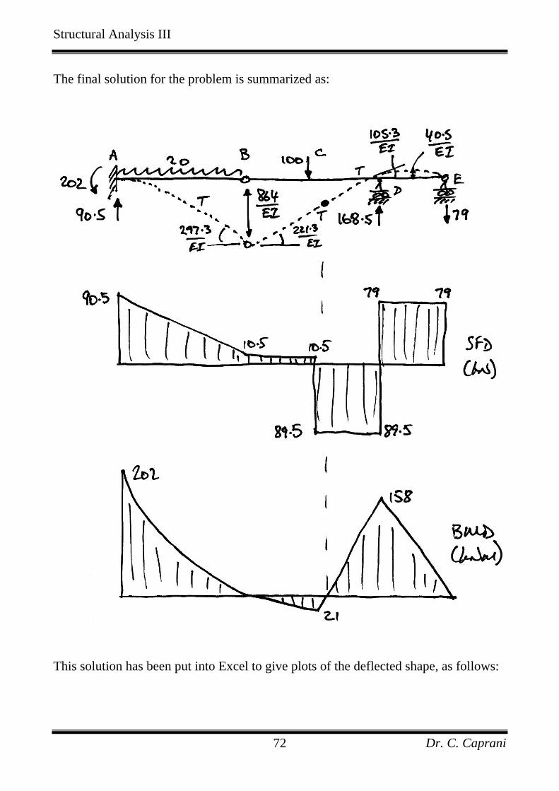
Dr. C. Caprani 72

The final solution for the problem is summarized as:

This solution has been put into Excel to give plots of the deflected shape, as follows:


Dr. C. Caprani 73

X global X for AB X for BE dy/dx AB y AB dy/dx BE y BE0.00 0.00 -4.00 0.0 0.0 305.3 -1861.30.25 0.25 -3.75 -47.7 -6.1 295.2 -1786.30.50 0.50 -3.50 -90.1 -23.4 285.6 -1713.70.75 0.75 -3.25 -127.5 -50.7 276.8 -1643.41.00 1.00 -3.00 -160.1 -86.8 268.6 -1575.21.25 1.25 -2.75 -188.3 -130.4 261.0 -1509.11.50 1.50 -2.50 -212.4 -180.6 254.1 -1444.71.75 1.75 -2.25 -232.8 -236.3 247.9 -1381.92.00 2.00 -2.00 -249.7 -296.7 242.3 -1320.72.25 2.25 -1.75 -263.4 -360.9 237.4 -1260.72.50 2.50 -1.50 -274.3 -428.1 233.1 -1201.92.75 2.75 -1.25 -282.6 -497.8 229.5 -1144.13.00 3.00 -1.00 -288.8 -569.3 226.6 -1087.13.25 3.25 -0.75 -293.0 -642.0 224.3 -1030.73.50 3.50 -0.50 -295.6 -715.6 222.6 -974.93.75 3.75 -0.25 -297.0 -789.7 221.7 -919.44.00 4.00 0.00 -297.3 -864.0 221.3 -864.04.25 0.25 0.0 0.0 221.7 -808.64.50 0.50 0.0 0.0 222.6 -753.14.75 0.75 0.0 0.0 224.3 -697.35.00 1.00 0.0 0.0 226.6 -640.95.25 1.25 0.0 0.0 229.5 -583.95.50 1.50 0.0 0.0 233.1 -526.15.75 1.75 0.0 0.0 237.4 -467.36.00 2.00 0.0 0.0 242.3 -407.36.25 2.25 0.0 0.0 244.8 -346.36.50 2.50 0.0 0.0 241.6 -285.46.75 2.75 0.0 0.0 232.9 -226.07.00 3.00 0.0 0.0 218.6 -169.47.25 3.25 0.0 0.0 198.7 -117.27.50 3.50 0.0 0.0 173.1 -70.67.75 3.75 0.0 0.0 142.0 -31.18.00 4.00 0.0 0.0 105.3 0.08.25 4.25 0.0 0.0 68.3 21.68.50 4.50 0.0 0.0 36.2 34.58.75 4.75 0.0 0.0 9.0 40.19.00 5.00 0.0 0.0 -13.2 39.59.25 5.25 0.0 0.0 -30.5 33.9 dy/dx AB = (80+V)*x^2/2-(160+4*V)*x-20*x^3/69.50 5.50 0.0 0.0 -42.8 24.7 y AB = (80+V)*x^3/6-(160+4*V)*x^2/2-20*x^4/249.75 5.75 0.0 0.0 -50.2 12.9 dy/dx BE = V*x^2/2+(200-3*V)*MAX(x-4,0)^2/2-100*MAX(x-2,0)^2/2+const110.00 6.00 0.0 0.0 -52.7 0.0 y BE = V*x^3/6+(200-3*V)*MAX(x-4,0)^3/6-100*MAX(x-2,0)^3/6+const1*x+const2

Macaulay's Method - Indeterminate Beam with Hinge

Equation used in the Cells

-400.0

-300.0

-200.0

-100.0

0.0

100.0

200.0

300.0

0.00 2.00 4.00 6.00 8.00 10.00

Distance Along Beam (m)

Rot

atio

n - (

dy/d

x)/E

I

dy/dx for AB

dy/dx for BE (4<x<10)

-1000.0

-900.0

-800.0

-700.0

-600.0

-500.0

-400.0

-300.0

-200.0

-100.0

0.0

100.0

0.00 2.00 4.00 6.00 8.00 10.00

Distance Along Beam (m)D

efle

ctio

n -y

/EI

y for ABy for BE (4<x<10)


Dr. C. Caprani 74

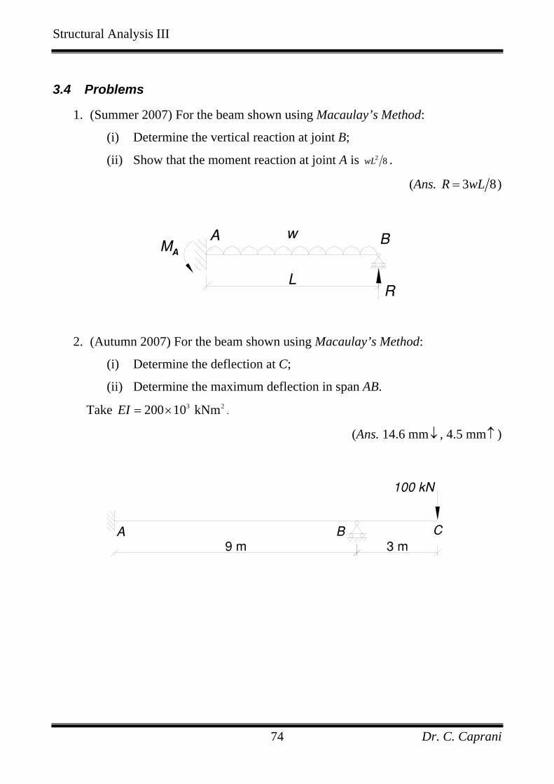
3.4 Problems

1. (Summer 2007) For the beam shown using Macaulay’s Method:

(i) Determine the vertical reaction at joint B;

(ii) Show that the moment reaction at joint A is 2 8wL .

(Ans. 3 8R wL= )

w

L

MA

A B

R

2. (Autumn 2007) For the beam shown using Macaulay’s Method:

(i) Determine the deflection at C;

(ii) Determine the maximum deflection in span AB.

Take 3 2200 10 kNmEI = × .

(Ans. 14.6 mm↓ , 4.5 mm↑ )

100 kN

A B9 m 3 m

C


Dr. C. Caprani 75

3. For the beam shown, find the reactions and draw the bending moment, shear

force, and deflected shape diagrams. Determine the maximum deflection and

rotation at B in terms of EI.








Dr. C. Caprani 76



the rotations at A, B, and C in terms of EI.



the rotations at A, B, and C in terms of EI.

8. (Summer 2008) For the prismatic beam of Fig. Q3(b), using Macaulay’s

Method, find the vertical deflection at C in terms of EI.

(Ans. 20 EI )

A B6 m 2 m

C

20 kN/m


Dr. C. Caprani 77

4. Indeterminate Frames

4.1 Introduction

Macaulay’s method is readily applicable to frames, just as it is to beams. Both

statically indeterminate and determinate frames can be solved. The method is applied

as usual, but there is one extra factor:

Compatibility of displacement must be maintained at joints.

This means that:

• At rigid joints, this means that the rotations of members meeting at the joint

must be the same.

• At hinge joints we can have different rotations for each member, but the

members must remain connected.

• We must (obviously) still impose the boundary conditions that the supports

offer the frame.

In practice, Macaulay’s Method is only applied to basic frames because the number

of equations gets large otherwise. For more complex frames other forms of analysis

can be used (such as moment distribution, virtual work, Mohr’s theorems, etc.) to

determine the bending moments. Once these are known, the defections along

individual members can then be found using Macaulay’s method applied to the

member itself.


Dr. C. Caprani 78

4.2 Example 8 – Simple Frame

For the following prismatic frame, find the horizontal deflection at C and draw the

bending moment diagram:

Before starting, assess the behaviour of the frame:

The structure is 1 degree indeterminate. Therefore we need to choose a redundant.

Choosing BV , we can now calculate the reactions in terms of the redundant by taking

moments about A:


Dr. C. Caprani 79

100 3 6 0

6 300A

A

M RM R

+ ⋅ − == −

Thus the reactions are:

And we can now draw a free-body diagram for member AB, in order to apply

Macaulay’s Method to AB:


( ) ( )[ ]06 300 0M x R x Rx− − + =


Dr. C. Caprani 80

Thus:

( ) ( )[ ]2

0

2 6 300d yM x EI R x Rxdx

= = − − Equation 1

Giving:

( )[ ]1 26 3002

dy REI R x x Cdx θ= − − + Equation 2

( ) [ ]2 36 3002 6

R REIy x x C x Cθ δ

−= − + + Equation 3

Applying 0y = and 0dydx

= at 0x = gives us 0Cθ = and 0Cδ = . Therefore:

( )[ ]1 26 3002

dy REI R x xdx

= − − Equation 4

( ) [ ]2 36 3002 6

R REIy x x−

= − Equation 5

Further, we know that at 6x = , 0y = because of support B. Therefore:

( ) ( ) ( ) ( )2 36 3000 6 6

2 60 3 150

75 kN i.e.

R REI

R RR

−= −

= − −

= + ↑

Thus we now have:


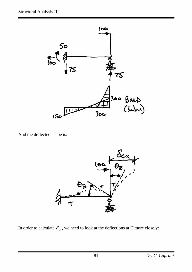
Dr. C. Caprani 81

And the deflected shape is:

In order to calculate Cxδ , we need to look at the deflections at C more closely:


Dr. C. Caprani 82

From this diagram, it is apparent that the deflection at C is made up of:

• A deflection due to the rotation of joint B, denoted Bθδ ;

• A deflection caused by bending of the cantilever member BC, cantiδ .

From S Rθ= , we know that:

3B Bθδ θ=

So to find Bθ we use Equation 4 with 6x = :

( ) ( )275150 6 6

2450

B

B

EI

EI

θ

θ

= −

−=

The sense of the rotation is thus as shown:


Dr. C. Caprani 83

The deflection at C due to the rotation of joint B is:

4503

1350

B EI

EI

θδ⎛ ⎞= ⎜ ⎟⎝ ⎠

=

Note that we don’t need to worry about the sign of the rotation, since we know that C

is moving to the right, and that the rotation at B is aiding this movement.

The cantilever deflection of member BC can be got from standard tables as:

3 3

canti

100 3 9003 3PLEI EI EI

δ ⋅= = =

We can also get this using Macaulay’s Method applied to member BC:

Note the following:


Dr. C. Caprani 84

• Applying Macaulay’s method to member BC will not give the deflection at C –

it will only give the deflection at C due to bending of member BC. Account

must be made of the rotation of joint B.

• The axis system for Macaulay’s method is as previously used, only turned

through 90 degrees. Thus negative deflections are to the right, as shown.

Taking moments about the cut:

( ) [ ]0300 100 0M x x x+ − =

( ) [ ]2

0

2 100 300d yM x EI x xdx

= = −

[ ]12100 3002

dyEI x x Cdx θ= − +

[ ]23100 3006 2

EIy x x C x Cθ δ= − + +

But we know that 0y = and 0dydx

= at 0x = so 0Cθ = and 0Cδ = . Therefore:

[ ]23100 3006 2

EIy x x= −

And for the cantilever deflection at C:


Dr. C. Caprani 85

( ) ( )3 2

canti

canti

100 3003 36 2

900

EI

EI

δ

δ

= −

−=

This is the same as the standard table result, as expected. Further, since a negative

answer here means a deflection to the right, the total deflection to the right at C is:

canti

1350 900

2250

Cx B

EI EI

EI

θδ δ δ= +

= +

=


Dr. C. Caprani 86

4.3 Problems

1. For the prismatic frame shown, find the reactions and draw the bending

moment, shear force, and deflected shape diagrams. Verify the following

displacements: 80B EIθ = ; 766.67Dy EIδ = ↓ ; 200Bx EIδ = (direction not

given because to do so would influence answer).

2. For the prismatic frame shown, find the reactions and draw the bending

moment, shear force, and deflected shape diagrams. Verify the following

displacements: 200C EIθ = ; 666.67By EIδ = ↓ ; 400Dx EIδ = (again

direction not given because to do so would influence answer).


Dr. C. Caprani 87

5. Appendix

5.1 References

The basic reference is the two-page paper which started it all:

• Macaulay, W. H. (1919), ‘Note on the deflection of the beams’, Messenger of

Mathematics, 48, pp. 129-130.

Most textbooks cover the application of the method, for example:

• Gere, J.M and Goodno, B.J. (2008), Mechanics of Materials, 7th Edn., Cengage

Engineering.

• McKenzie, W.M.C. (2006), Examples in Structural Analysis, Taylor and

Francis, Abington.

• Benham, P.P., Crawford, R.J. and Armstrong, C.G. (1996), Mechanics of

Engineering Materials, 2nd Edn., Pearson Education.

Some interesting developments and uses of the step-functions method are:

• Biondi, B. and Caddemi, S. (2007), ‘Euler–Bernoulli beams with multiple

singularities in the flexural stiffness’, European Journal of Mechanics A/Solids,

26 pp. 789–809.

• Falsone, G. (2002), ‘The use of generalised functions in the discontinuous beam

bending differential equations’, International Journal of Engineering

Education, Vol. 18, No. 3, pp. 337-343.

See www.colincaprani.com for notes on the use of Macaulay’s Method in the

development of a general beam analysis program, based upon the following work:

• Wilson, H.B., Turcotte, L.H., and Halpern, D. (2003), Advanced Mathematics

and Mechanics Applications Using MATLAB, 3rd Edn., Chapman and

Hall/CRC, Boca Raton, Florida.

Documents

Macaulay's Method 0809