LYAPUNOV DESIGN

S.S. Ge, Department of Electrical and Computer Engineering, The National University of

Singapore, Singapore

Keywords: Control Lyapunov Function, Lyapunov Design, Model Reference Adaptive Con-

trol, Adaptive Control, Backstepping Design.

Contents

1. Introduction

2. Control Lyapunov Function

3. Lyapunov Design via Lyapunov Equation

3.1. Lyapunov Equation

3.2. MRAC for Linear Time Invariant Systems

3.3. MRAC for Nonlinear Systems

4. Lyapunov Design for Matched and Unmatched Uncertainties

4.1. Lyapunov Design for Systems with Matched Uncertainties

4.1.1. Lyapunov Redesign

4.1.2. Adaptive Lyapunov Redesign

4.1.3. Robust Lyapunov Redesign

4.2. Backstepping Design for Systems with Unmatched Uncertainties

4.2.1. Backstepping for Known Parameter Case

4.2.2. Adaptive Backstepping for Unknown Parameter Case

4.2.3. Adaptive Backstepping with Tuning Function

5. Property-based Lyapunov Design

5.1. Physically Motivated Lyapunov Design

5.2. Integral Lyapunov Function for Nonlinear Parameterizations

6. Design Flexibilities and Considerations

7. Conclusions

Bibliography

Glossary

Lipschitz continuity: The function f(x; t) is said to be Lipschitz continuous in x, if for some

h > 0, there exists L � 0 such that jf(x1; t)�f(x2; t)j � Ljx1�x2j for all x1, x2 2 B(0; t),

t > 0 where B(0; h) is the ball of radius h centered at 0. The constant L is called the

Lipschitz constant.

Equilibrium point: x� is said to be an equilibrium point of system _x = f(x; t);x(t0) = x0 if

f(x�; t) = 0 for all t � 0.

Stable equilibrium: An equilibrium point where all solutions starting at nearby points stay

nearby. The equilibrium state x = 0 is said to be stable if, for any � > 0 and t0 � 0,

there exists a Æ(�; t0) such that if jx(t0)j < Æ(�; t0), then jx(t)j < � for all t > t0.

Uniformly stable: The equilibrium point x = 0 is uniformly stable if Æ is the de�nition of

stable equilibrium can be chosen independent of t0.

Region of attraction: The set of all points with the property that the trajectories starting

at these points asymptotically converge to the origin.

Asymptotic stability: The equilibrium point x = 0 is an asymptotically stable equilibrium

point of system _x = f(x; t) if (i) x = 0 is a stable equilibrium point; and (ii) x = 0 is

attractive, that is for all t0 � 0 there exists Æ(t0) such that jx0j < Æ ! limt!1 jx(t)j = 0,

i.e., all trajectories starting at nearby points approach the equilibrium point as time goes

to in�nity.

Hurwitz matrix: A square real matrix is Hurwitz if all its eigenvalues have negative real

parts.

Positive (semi-) de�nite function: A scalar function of a vector argument V (x) is positive

(semi-) de�nite if it vanishes at the origin and is positive (nonnegative) for all points in

the neighborhood of the origin, excluding the origin.

Positive (semi-) de�nite matrix: A square symmetric real matrix P is positive (semi-) def-

inite if the quadratic form V (x) = xTPx is a positive (semi-) de�nite function.

Negative (semi-) de�nite function: A scalar function of a vector argument V (x) is nega-

tive (semi-) de�nite if it vanishes at the origin and is negative (nonpositive) for all points

in the neighborhood of the origin, excluding the origin.

Negative (semi-) de�nite matrix: A square symmetric real matrix P is negative (semi-)

de�nite if the quadratic form V (x) = xTPx is a negative (semi-) de�nite function.

Lyapunov equation: A linear algebraic matrix equation of the form PA+ATP = �Q, where

A and Q are real square matrices and Q is symmetric and positive de�nite. The equation

has a (unique) positive de�nite matrix solution P if and only if A is Hurwitz.

Lyapunov function (LF): A scalar positive de�nite function V (x) of the states whose deriva-

tive along the trajectories of the system is negative de�nite.

Control Lyapunov Function: A scalar smooth positive de�nite and radially unbounded

function V (x) : Rn ! R+ is called a Control Lyapunov Function (CLF) for control

system _x = f(x;u) there exists u(x) such that@V (x)

@xf(x;u(x)) < 0 8x 6= 0.

Invariant Set: : A set is an invariant set for a dynamic system if every system trajectory

which starts from a point in remains in for all future time.

Ln2 : Let x(t) 2 R

n be a continuous or piecewise continuous vector function. Then the 2� norm

space is de�ned as Ln2 =: fx : jkxk2 =

R1

0xTxdt <1g.

Ln1: Let x(t) 2 R

n be a continuous or piecewise continuous vector function. Then the 1�norm space is de�ned as Ln

1=: fx : jkxk1 = max1�i�n jxij <1g.

diag[�]: Diagonal matrix with given diagonal elements.

inf �(t): The largest number that is smaller than or equal to the minimum value of �(t).

�max(A): The maximum eigenvalue of A, where �max(A) is real.

Summary

This article gives an overview on some state-of-the-art approaches of Lyapunov design by divid-

ing systems into several distinct classes, though in general there is no systematic procedure in

choosing a suitable Lyapunov function candidate for controller design to guarantee the closed-

loop stability for a given nonlinear system. After a brief introduction and historic review, this

article sequentially presents (i) the basic concepts of Lyapunov stability and control Lyapunov

functions, (ii) Lyapunov equations and model reference adaptive control based on Lyapunov

design for matched systems, (iii) Lyapunov redesign, adaptive redesign and robust design for

matched systems, (iv) adaptive backstepping design for unmatched nonlinear systems, (v) Lya-

punov design by exploiting physical properties for special classes of systems, and (vi) design

exibilities and considerations in actual design.

1. Introduction

Lyapunov design has been a primary tool for nonlinear control system design, stability and

performance analysis since its introduction in 1982. The basic idea is to design a feedback

control law that renders the derivative of a speci�ed Lyapunov function candidate negative

de�nite or negative semi-de�nite. Lyapunov's direct method is a mathematical interpretation

of the physical property that if a system's total energy is dissipating, then the states of the

system will ultimately reach to an equilibrium point. The basic idea behind the method is that,

if there exists a kind of continuous scalar \energy" function such that this \energy" diminishes

along the system's trajectory, then the system is said to be asymptotically stable. Since there is

no need to solve the solution of the di�erential equations governing the system in determining

its stability, it is usually referred to as the direct method (see Lyapunov Stability).

Although Lyapunov direct method is eÆcient for stability analysis, it is of restricted applica-

bility due to the diÆculty in selecting a Lyapunov function. The situation is di�erent when

facing the controller design problem, where the control has not being speci�ed, and the system

under consideration is undetermined. Lyapunov functions have been e�ectively utilized in the

synthesis of control systems. The basic idea is that, by �rst choosing a Lyapunov function

candidate and then the feedback control law can be speci�ed such that it renders the derivative

of the speci�ed Lyapunov function candidate negative de�nite, or negative semi-de�nite when

invariance principle can be used to prove asymptotic stability. This way of designing control

is called Lyapunov design. Lyapunov design depends on the selection of Lyapunov function

candidates. Though the result is suÆcient, it is a diÆcult problem to �nd a Lyapunov func-

tion (LF) satisfying the requirements of Lyapunov design. Fortunately, during the past several

decades, many e�ective control design approaches have been developed for di�erent classes of

linear and nonlinear systems based on the basic ideas of Lyapunov design. Lyapunov functions

are additive, like energy, i.e., Lyapunov functions for combinations of subsystems may be de-

rived by adding the Lyapunov functions of the subsystems. This point can be seen clearly in

the adaptive control design and backstepping design in this article.

Though Lyapunov design is a very powerful tools for control system design, stability and

performance analysis, the construction of a Lyapunov function is not easy for general nonlinear

systems, and it is usually a trial-and-error process and there is a lack of systematic methods.

Di�erent choices of Lyapunov functions may result in di�erent control structures and control

performance. Past experience shows that a good design of Lyapunov function should fully

utilize the property of the studied systems. Lyapunov design is used in many contexts, such as

dynamic feedback, output-feedback, estimation of region of attraction, and adaptive control,

among others. The article is not meant to be comprehensive but to serve as an introduction

to the state-of-the-art of full-state feedback design based on Lyapunov techniques for several

typical classes of autonomous systems.

Intensive research in adaptive control was �rst motivated for the design of autopilots for high

performance aircraft in the early 1950s because their dynamics change drastically when they

y from one operating point to another and constant gain feedback control cannot handle it

e�ectively. The lack of stability theory and one disastrous ight test led to the diminishing

interest in adaptive control in the late 1950s. The 1960s saw many advances in control theory

and adaptive control in particular. Simultaneous development in computers and electronics

that made the implementation of complex controllers possible, interest in adaptive control and

its applications was renewed in the 1970s and several breakthrough results were made. The

uncover of nonrobust behaviour of adaptive control subject to small disturbance and unmod-

elled dynamics in 1979 and the earlier 1980s, it led to better understanding of the instability

mechanisms and the design of robust adaptive control in the later 1980s though it was very

controversial initially. They were all systems satisfying the matching condition. In the later

1980s and earlier 1990s, the matching condition was relaxed to the extended matching condition,

which for one period was regarded as the frontier that could not be crossed by Lyapunov design,

and then further relaxed to the strict-feedback systems with general unmatched uncertainties

through backstepping design, which is the state-of-the-art of adaptive control.

This article gives an overview of the state-of-the-art approaches of Lyapunov design and ways

of choosing Lyapunov functions in the area of full-state adaptive control. Section 2 presents the

concepts of Lyapunov stability analysis and control Lyapunov functions. In Section 3, Lyapunov

functions for linear time invariant systems are presented �rst, then the results are utilized to

solve Model Reference Adaptive Control (MRAC) problems for classes of linear and nonlinear

systems which can be transformed to systems having stable linear portion. For this class of

problems, the choice of Lyapunov functions is systematic and controller design is standard. In

Section 4, after the presentation of Lyapunov Redesign, Adaptive Lyapunov Redesign, Robust

Lyapunov Redesign for a class of matched systems, backstepping controller design is discussed

for unmatched nonlinear systems. By exploiting the physical properties of the systems under

study, Section 5 shows that di�erent choices of Lyapunov functions and better controllers are

possible. Section 6 discusses the design exibilities and considerations in actual applications of

Lyapunov design, and further research work.

2. Control Lyapunov Function

Though Lyapunov's method applies to nonautonomous systems _x = f(x; t), for clarity and

simplicity, we shall restrain our discussion to time-invariant nonlinear systems of the form

_x = f(x) (1)

where x 2 Rn, and f(x) : Rn ! R

n is continuous. The basic idea of Lyapunov direct method

consists of (ii) choosing a radially unbounded positive de�nite Lyapunov function candidate

V (x), and (ii) evaluating its derivative _V (x) along system dynamics (1) and checking its neg-

ativeness for stability analysis.

Lyapunov design refers to the synthesis of control laws for some desired closed-loop stability

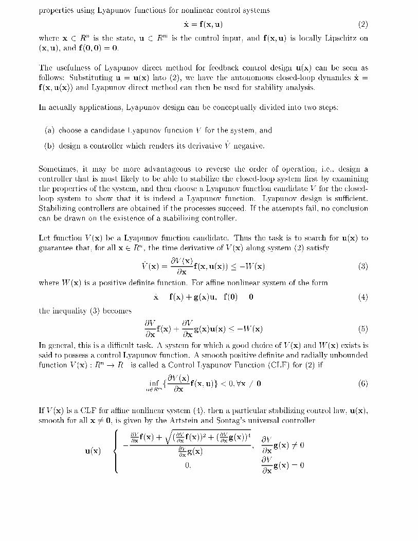
properties using Lyapunov functions for nonlinear control systems

_x = f(x;u) (2)

where x 2 Rn is the state, u 2 R

m is the control input, and f(x;u) is locally Lipschitz on

(x;u), and f(0; 0) = 0.

The usefulness of Lyapunov direct method for feedback control design u(x) can be seen as

follows: Substituting u = u(x) into (2), we have the autonomous closed-loop dynamics _x =

f(x;u(x)) and Lyapunov direct method can then be used for stability analysis.

In actually applications, Lyapunov design can be conceptually divided into two steps:

(a) choose a candidate Lyapunov function V for the system, and

(b) design a controller which renders its derivative _V negative.

Sometimes, it may be more advantageous to reverse the order of operation, i.e., design a

controller that is most likely to be able to stabilize the closed-loop system �rst by examining

the properties of the system, and then choose a Lyapunov function candidate V for the closed-

loop system to show that it is indeed a Lyapunov function. Lyapunov design is suÆcient.

Stabilizing controllers are obtained if the processes succeed. If the attempts fail, no conclusion

can be drawn on the existence of a stabilizing controller.

Let function V (x) be a Lyapunov function candidate. Thus the task is to search for u(x) to

guarantee that, for all x 2 Rn, the time derivative of V (x) along system (2) satisfy

_V (x) =

@V (x)

@xf(x;u(x)) � �W (x) (3)

where W (x) is a positive de�nite function. For aÆne nonlinear system of the form

_x = f(x) + g(x)u; f(0) = 0 (4)

the inequality (3) becomes

@V

@xf(x) +

@V

@xg(x)u(x) � �W (x) (5)

In general, this is a diÆcult task. A system for which a good choice of V (x) and W (x) exists is

said to possess a control Lyapunov function. A smooth positive de�nite and radially unbounded

function V (x) : Rn ! R+ is called a Control Lyapunov Function (CLF) for (2) if

infu2Rm

f@V (x)@x

f(x;u)g < 0; 8x 6= 0 (6)

If V (x) is a CLF for aÆne nonlinear system (4), then a particular stabilizing control law, u(x),

smooth for all x 6= 0, is given by the Artstein and Sontag's universal controller

u(x) =

8>>><>>>:

�@V

@xf(x) +

q(@V@xf(x))2 + (@V

@xg(x))4

@V

@xg(x)

;

@V

@xg(x) 6= 0

0;@V

@xg(x) = 0

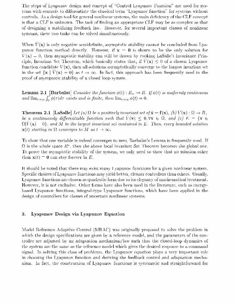
The steps of Lyapunov design and concept of \Control Lyapunov Function" are used for sys-

tems with controls to di�erentiate the classical term \Lyapunov function" for systems without

controls. As a design tool for general nonlinear systems, the main de�ciency of the CLF concept

is that a CLF is unknown. The task of �nding an appropriate CLF may be as complex as that

of designing a stabilizing feedback law. However, for several important classes of nonlinear

systems, these two tasks can be solved simultaneously.

When _V (x) is only negative semide�nite, asymptotic stability cannot be concluded from Lya-

punov function method directly. However, if x = 0 is shown to be the only solution for_V (x) = 0, then asymptotic stability can still be drawn by evoking LaSalle's Invariance Prin-

ciple, Invariant Set Theorem, which basically states that, if _V (x) � 0 of a chosen Lyapunov

function candidate V (x), then all solutions asymptotically converge to the largest invariant set

in the set fx j _V (x) = 0g as t ! 1. In fact, this approach has been frequently used in the

proof of asymptotic stability of a closed-loop system.

Lemma 2.1 [Barbalat] Consider the function �(t) : R+ ! R. If �(t) is uniformly continuous

and limt!1

R t

0�(�)d� exists and is �nite, then limt!1 �(t) = 0.

Theorem 2.1 [LaSalle] Let (a) be a positively invariant set of _x = f(x), (b) V (x) : ! R+

be a continuously di�erentiable function such that _V (x) � 0; 8x 2 , and (c) E = fx 2

j _V (x) = 0g, and M be the largest invariant set contained in E. Then, every bounded solution

x(t) starting in converges to M as t!1.

To show that one variable is indeed converges to zero, Barbalat's Lemma is frequently used. If

is the whole space Rn, then the above local Invariant Set Theorem becomes the global one.

To prove the asymptotic stability of the system, we only need to show that no solution other

than x(t) � 0 can stay forever in E.

It should be noted that there may exist many Lyapunov functions for a given nonlinear system.

Speci�c choices of Lyapunov functions may yield better, cleaner controllers than others. Usually,

Lyapunov functions are chosen as quadratic form due to its elegancy of mathematical treatment.

However, it is not exclusive. Other forms have also been used in the literature, such as energy-

based Lyapunov functions, integral-type Lyapunov functions, which have been applied in the

design of controllers for classes of uncertain nonlinear systems.

3. Lyapunov Design via Lyapunov Equation

Model Reference Adaptive Control (MRAC) was originally proposed to solve the problem in

which the design speci�cations are given by a reference model, and the parameters of the con-

troller are adjusted by an adaptation mechanism/law such that the closed-loop dynamics of

the system are the same as the reference model which gives the desired response to a command

signal. In solving this class of problems, the Lyapunov equation plays a very important role

in choosing the Lyapunov function and deriving the feedback control and adaptation mecha-

nism. In fact, the construction of Lyapunov functions is systematic and straightforward for

the class of systems which can be transformed into two portions: (i) a stable linear portion so

that linear stability results can be directly applied, and (ii) matched nonlinear portion which

can be handled using di�erent techniques such as adaptive or robust control techniques in dif-

ferent situations. Thus, MRAC can also be viewed as Lyapunov design based on Lyapunov

equations. To explain the concepts clearly, Lyapunov equation and Lyapunov stability analysis

are �rstly presented for linear time-invariant systems, then adaptive control design for classes

of unknown linear time invariant systems and unknown nonlinear systems are presented by

utilizing Lyapunov equation.

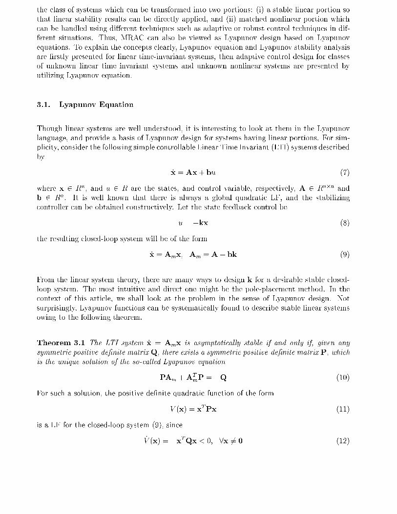
3.1. Lyapunov Equation

Though linear systems are well understood, it is interesting to look at them in the Lyapunov

language, and provide a basis of Lyapunov design for systems having linear portions. For sim-

plicity, consider the following simple controllable Linear Time Invariant (LTI) systems described

by

_x = Ax+ bu (7)

where x 2 Rn, and u 2 R are the states, and control variable, respectively, A 2 R

n�n and

b 2 Rn. It is well known that there is always a global quadratic LF, and the stabilizing

controller can be obtained constructively. Let the state feedback control be

u = �kx (8)

the resulting closed-loop system will be of the form

_x = Amx; Am = A� bk (9)

From the linear system theory, there are many ways to design k for a desirable stable closed-

loop system. The most intuitive and direct one might be the pole-placement method. In the

context of this article, we shall look at the problem in the sense of Lyapunov design. Not

surprisingly, Lyapunov functions can be systematically found to describe stable linear systems

owing to the following theorem.

Theorem 3.1 The LTI system _x = Amx is asymptotically stable if and only if, given any

symmetric positive-de�nite matrix Q, there exists a symmetric positive-de�nite matrix P, which

is the unique solution of the so-called Lyapunov equation

PAm +ATmP = �Q (10)

For such a solution, the positive de�nite quadratic function of the form

V (x) = xTPx (11)

is a LF for the closed-loop system (9), since

_V (x) = �xTQx < 0; 8x 6= 0 (12)

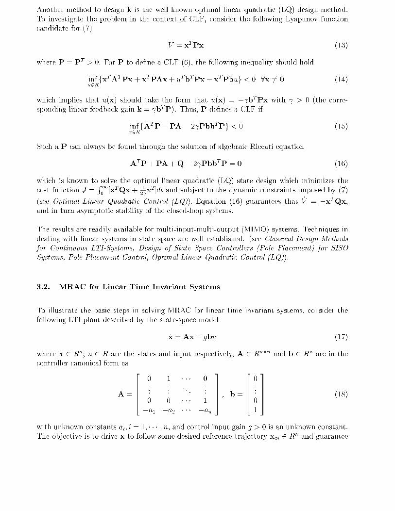
Another method to design k is the well known optimal linear quadratic (LQ) design method.

To investigate the problem in the context of CLF, consider the following Lyapunov function

candidate for (7)

V = xTPx (13)

where P = PT> 0. For P to de�ne a CLF (6), the following inequality should hold

infu2R

fxTATPx+ xTPAx+ uTbTPx+ xTPbug < 0 8x 6= 0 (14)

which implies that u(x) should take the form that u(x) = � bTPx with > 0 (the corre-

sponding linear feedback gain k = bTP). Thus, P de�nes a CLF if

inf 2R

fATP+PA� 2 PbbTPg < 0 (15)

Such a P can always be found through the solution of algebraic Riccati equation

ATP+PA+Q� 2 PbbTP = 0 (16)

which is known to solve the optimal linear quadratic (LQ) state design which minimizes the

cost function J =R1

0[xTQx + 1

2 u2]dt and subject to the dynamic constraints imposed by (7)

(see Optimal Linear Quadratic Control (LQ)). Equation (16) guarantees that _V = �xTQx,

and in turn asymptotic stability of the closed-loop systems.

The results are readily available for multi-input-multi-output (MIMO) systems. Techniques in

dealing with linear systems in state space are well established. (see Classical Design Methods

for Continuous LTI-Systems, Design of State Space Controllers (Pole Placement) for SISO

Systems, Pole Placement Control, Optimal Linear Quadratic Control (LQ)).

3.2. MRAC for Linear Time Invariant Systems

To illustrate the basic steps in solving MRAC for linear time invariant systems, consider the

following LTI plant described by the state-space model

_x = Ax+ gbu (17)

where x 2 Rn; u 2 R are the states and input respectively, A 2 R

n�n and b 2 Rn are in the

controller canonical form as

A =

26664

0 1 � � � 0...

.... . .

...

0 0 � � � 1

�a1 �a2 � � � �an

37775 ; b =

266640...

0

1

37775 (18)

with unknown constants ai; i = 1; � � � ; n, and control input gain g > 0 is an unknown constant.

The objective is to drive x to follow some desired reference trajectory xm 2 Rn and guarantee

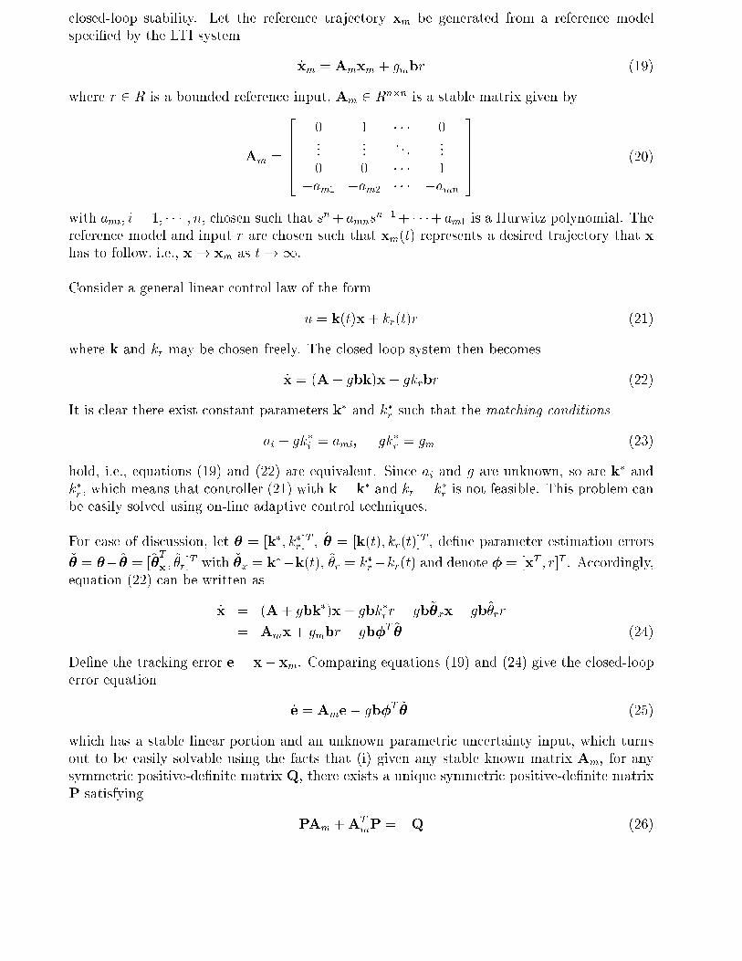
closed-loop stability. Let the reference trajectory xm be generated from a reference model

speci�ed by the LTI system

_xm = Amxm + gmbr (19)

where r 2 R is a bounded reference input, Am 2 Rn�n is a stable matrix given by

Am =

26664

0 1 � � � 0...

.... . .

...

0 0 � � � 1

�am1 �am2 � � � �amn

37775 (20)

with ami; i = 1; � � � ; n, chosen such that sn+ amnsn�1+ � � �+ am1 is a Hurwitz polynomial. The

reference model and input r are chosen such that xm(t) represents a desired trajectory that x

has to follow, i.e., x! xm as t!1.

Consider a general linear control law of the form

u = k(t)x+ kr(t)r (21)

where k and kr may be chosen freely. The closed-loop system then becomes

_x = (A+ gbk)x+ gkrbr (22)

It is clear there exist constant parameters k� and k�

r such that the matching conditions

ai + gk�

i = ami; gk�

r = gm (23)

hold, i.e., equations (19) and (22) are equivalent. Since ai and g are unknown, so are k� and

k�

r , which means that controller (21) with k = k� and kr = k�

r is not feasible. This problem can

be easily solved using on-line adaptive control techniques.

For ease of discussion, let � = [k�; k�r ]T , �̂ = [k(t); kr(t)]

T , de�ne parameter estimation errors

~� = �� �̂ = [~�T

x;~�r]

T with ~�x = k��k(t), ~�r = k�

r�kr(t) and denote � = [xT ; r]T . Accordingly,

equation (22) can be written as

_x = (A+ gbk�)x + gbk�rr � gb~�xx� gb~�rr

= Amx+ gmbr � gb�T ~� (24)

De�ne the tracking error e = x� xm. Comparing equations (19) and (24) give the closed-loop

error equation

_e = Ame� gb�T ~� (25)

which has a stable linear portion and an unknown parametric uncertainty input, which turns

out to be easily solvable using the facts that (i) given any stable known matrix Am, for any

symmetric positive-de�nite matrix Q, there exists a unique symmetric positive-de�nite matrix

P satisfying

PAm +ATmP = �Q (26)

as detailed in Subsection 3.1, and (ii) the linear-in-the-parameter uncertainty b�T ~� can be

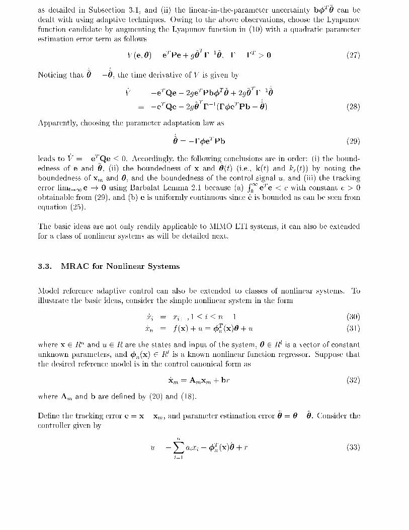
dealt with using adaptive techniques. Owing to the above observations, choose the Lyapunov

function candidate by augmenting the Lyapunov function in (10) with a quadratic parameter

estimation error term as follows

V (e; �) = eTPe+ g~�T��1~�; � = �T

> 0 (27)

Noticing that_~� = � _̂

�, the time derivative of V is given by

_V = �eTQe� 2geTPb�T ~� + 2g~�

T��1

_~�

= �eTQe� 2g~�T��1(��eTPb� _̂

�) (28)

Apparently, choosing the parameter adaptation law as

_̂� = ���eTPb (29)

leads to _V = �eTQe � 0. Accordingly, the following conclusions are in order: (i) the bound-

edness of e and ~�, (ii) the boundedness of x and �̂(t) (i.e., k(t) and kr(t)) by noting the

boundedness of xm and �, and the boundedness of the control signal u, and (iii) the tracking

error limt!1 e ! 0 using Barbalat Lemma 2.1 because (a)R1

0eTe < c with constant c > 0

obtainable from (29), and (b) e is uniformly continuous since _e is bounded as can be seen from

equation (25).

The basic ideas are not only readily applicable to MIMO LTI systems, it can also be extended

for a class of nonlinear systems as will be detailed next.

3.3. MRAC for Nonlinear Systems

Model reference adaptive control can also be extended to classes of nonlinear systems. To

illustrate the basic ideas, consider the simple nonlinear system in the form

_xi = xi+1; 1 � i � n� 1 (30)

_xn = f(x) + u = �Tn (x)� + u (31)

where x 2 Rn and u 2 R are the states and input of the system, � 2 R

l is a vector of constant

unknown parameters, and �n(x) 2 Rl is a known nonlinear function regressor. Suppose that

the desired reference model is in the control canonical form as

_xm = Amxm + br (32)

where Am and b are de�ned by (20) and (18).

De�ne the tracking error e = x� xm, and parameter estimation error ~� = �� �̂. Consider the

controller given by

u = �nXi=1

aixi � �Tn (x)�̂ + r (33)

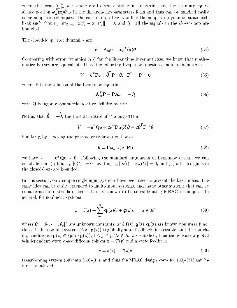
where the termsPn

i=1 aixi and r are to form a stable linear portion, and the certainty equiv-

alence portion �Tn (x)�̂ is in the linear-in-the-parameters form and thus can be handled easily

using adaptive techniques. The control objective is to �nd the adaptive (dynamic) state feed-

back such that (i) limt!1 kx(t) � xm(t)k = 0, and (ii) all the signals in the closed-loop are

bounded.

The closed-loop error dynamics are

_e = Ame+ b�Tn (x)

~� (34)

Comparing with error dynamics (25) for the linear time invariant case, we know that mathe-

matically they are equivalent. Thus, the following Lyapunov function candidate is in order

V = eTPe+ ~�T��1~�; �T = � > 0 (35)

where P is the solution of the Lyapunov equation

ATmP+PAm = �Q (36)

with Q being any symmetric positive de�nite matrix.

Noting that_~� = � _̂

�, the time derivative of V along (34) is

_V = �eTQe+ 2eTPb�T

n~� � 2~�

T��1

_̂� (37)

Similarly, by choosing the parameters adaptation law as

_̂� = ��n(x)e

TPb (38)

we have _V = �eTQe � 0. Following the standard arguments of Lyapunov design, we can

conclude that (i) limt!1 ke(t)k = 0, i.e., limt!1 kx(t)� xm(t)k = 0, and (ii) all the signals in

the closed-loop are bounded.

In this section, only simple single input systems have been used to present the basic ideas. The

same idea can be easily extended to multi-input systems, and many other systems that can be

transformed into standard forms that are known to be solvable using MRAC techniques. In

general, for nonlinear systems

_z = f(z) +

pXi=1

qi(z)�i + g(z)v; z 2 Rn (39)

where � = [�1; � � � ; �p]T are unknown constants, and f(z); g(z);qi(z) are known nonlinear func-

tions. If the nominal system (f(z); g(z)) is globally state feedback linearizable, and the match-

ing conditions qj(z) 2 spanfg(z)g; 1 � j � p; 8z 2 Rn are satis�ed, then there exists a global

�-independent state space di�eomorphism x = T (z) and a state feedback

v = k(z) + �(z)u (40)

transforming system (39) into (30)-(31), and thus the MRAC design steps for (30)-(31) can be

directly utilized.

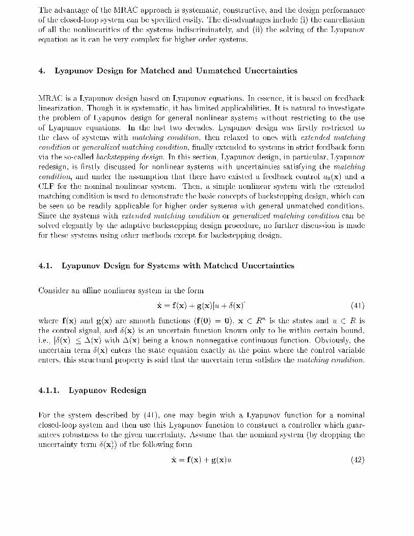
The advantage of the MRAC approach is systematic, constructive, and the design performance

of the closed-loop system can be speci�ed easily. The disadvantages include (i) the cancellation

of all the nonlinearities of the systems indiscriminately, and (ii) the solving of the Lyapunov

equation as it can be very complex for higher order systems.

4. Lyapunov Design for Matched and Unmatched Uncertainties

MRAC is a Lyapunov design based on Lyapunov equations. In essence, it is based on feedback

linearization. Though it is systematic, it has limited applicabilities. It is natural to investigate

the problem of Lyapunov design for general nonlinear systems without restricting to the use

of Lyapunov equations. In the last two decades, Lyapunov design was �rstly restricted to

the class of systems with matching condition, then relaxed to ones with extended matching

condition or generalized matching condition, �nally extended to systems in strict feedback form

via the so-called backstepping design. In this section, Lyapunov design, in particular, Lyapunov

redesign, is �rstly discussed for nonlinear systems with uncertainties satisfying the matching

condition, and under the assumption that there have existed a feedback control u0(x) and a

CLF for the nominal nonlinear system. Then, a simple nonlinear system with the extended

matching condition is used to demonstrate the basic concepts of backstepping design, which can

be seen to be readily applicable for higher order systems with general unmatched conditions.

Since the systems with extended matching condition or generalized matching condition can be

solved elegantly by the adaptive backstepping design procedure, no further discussion is made

for these systems using other methods except for backstepping design.

4.1. Lyapunov Design for Systems with Matched Uncertainties

Consider an aÆne nonlinear system in the form

_x = f(x) + g(x)[u+ Æ(x)] (41)

where f(x) and g(x) are smooth functions (f(0) = 0), x 2 Rn is the states and u 2 R is

the control signal, and Æ(x) is an uncertain function known only to lie within certain bound,

i.e., jÆ(x)j � �(x) with �(x) being a known nonnegative continuous function. Obviously, the

uncertain term Æ(x) enters the state equation exactly at the point where the control variable

enters, this structural property is said that the uncertain term satis�es the matching condition.

4.1.1. Lyapunov Redesign

For the system described by (41), one may begin with a Lyapunov function for a nominal

closed-loop system and then use this Lyapunov function to construct a controller which guar-

antees robustness to the given uncertainty. Assume that the nominal system (by dropping the

uncertainty term Æ(x)) of the following form

_x = f(x) + g(x)u (42)

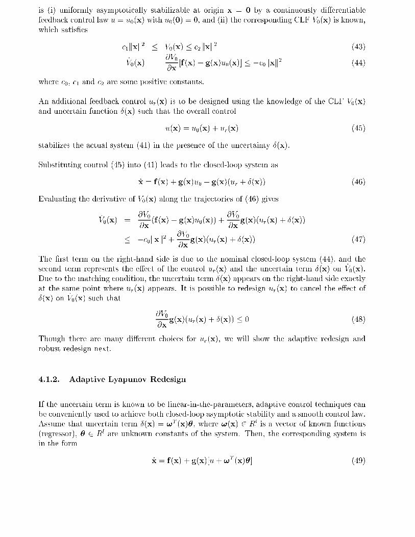
is (i) uniformly asymptotically stabilizable at origin x = 0 by a continuously di�erentiable

feedback control law u = u0(x) with u0(0) = 0, and (ii) the corresponding CLF V0(x) is known,

which satis�es

c1kxk2 � V0(x) � c2kxk2 (43)

_V0(x) =

@V0

@x[f(x) + g(x)u0(x)] � �c0kxk2 (44)

where c0, c1 and c2 are some positive constants.

An additional feedback control ur(x) is to be designed using the knowledge of the CLF V0(x)

and uncertain function Æ(x) such that the overall control

u(x) = u0(x) + ur(x) (45)

stabilizes the actual system (41) in the presence of the uncertainty Æ(x).

Substituting control (45) into (41) leads to the closed-loop system as

_x = f(x) + g(x)u0 + g(x)(ur + Æ(x)) (46)

Evaluating the derivative of V0(x) along the trajectories of (46) gives

_V0(x) =

@V0

@x(f(x) + g(x)u0(x)) +

@V0

@xg(x)(ur(x) + Æ(x))

� �c0kxk2 +@V0

@xg(x)(ur(x) + Æ(x)) (47)

The �rst term on the right-hand side is due to the nominal closed-loop system (44), and the

second term represents the e�ect of the control ur(x) and the uncertain term Æ(x) on _V0(x).

Due to the matching condition, the uncertain term Æ(x) appears on the right-hand side exactly

at the same point where ur(x) appears. It is possible to redesign ur(x) to cancel the e�ect of

Æ(x) on _V0(x) such that

@V0

@xg(x)(ur(x) + Æ(x)) � 0 (48)

Though there are many di�erent choices for ur(x), we will show the adaptive redesign and

robust redesign next.

4.1.2. Adaptive Lyapunov Redesign

If the uncertain term is known to be linear-in-the-parameters, adaptive control techniques can

be conveniently used to achieve both closed-loop asymptotic stability and a smooth control law.

Assume that uncertain term Æ(x) = !T (x)�, where !(x) 2 Rl is a vector of known functions

(regressor), � 2 Rl are unknown constants of the system. Then, the corresponding system is

in the form

_x = f(x) + g(x)[u+ !T (x)�] (49)

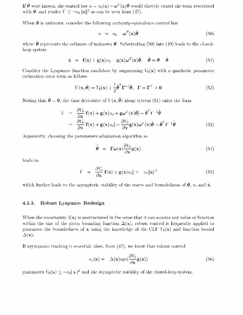
If � were known, the control law u = u0(x)�!T (x)� would directly cancel the term associated

with �, and render _V � �c0kxk2 as can be seen from (47).

When � is unknown, consider the following certainty-equivalence control law

u = u0 � !T (x)�̂ (50)

where �̂ represents the estimate of unknown �. Substituting (50) into (49) leads to the closed-

loop system

_x = f(x) + g(x)u0 + g(x)!T (x)~�; ~� = � � �̂ (51)

Consider the Lyapunov function candidate by augmenting V0(x) with a quadratic parameter

estimation error term as follows

V (x; ~�) = V0(x) +1

2~�T��1~�; � = �T

> 0 (52)

Noting that _� = 0, the time derivative of V (x; ~�) along system (51) takes the form

_V =

@V0

@x[f(x) + g(x)u0 + g!T (x)~�] + ~�

T��1

_~�

=@V0

@x[f(x) + g(x)u0] +

@V0

@xg(x)!T (x)~� � ~�

T��1

_̂� (53)

Apparently, choosing the parameters adaptation algorithm as

_̂� = �!(x)

@V0

@xg(x) (54)

leads to

_V =

@V0

@x[f(x) + g(x)u0] � �c0kxk2 (55)

which further leads to the asymptotic stability of the states and boundedness of �̂, u, and _x.

4.1.3. Robust Lyapunov Redesign

When the uncertainty Æ(x) is unstructured in the sense that it can assume any value or function

within the size of the given bounding function �(x), robust control is frequently applied to

guarantee the boundedness of x using the knowledge of the CLF V0(x) and function bound

�(x).

If asymptotic tracking is essential, then, from (47), we know that robust control

ur(x) = ��(x)sgn(@V0@x

g(x)) (56)

guarantees _V0(x) � �c0kxk2 and the asymptotic stability of the closed-loop system.

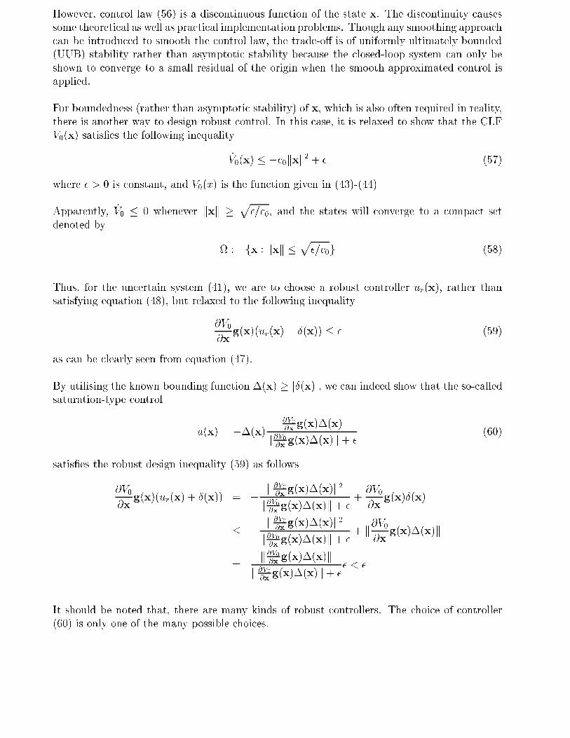
However, control law (56) is a discontinuous function of the state x. The discontinuity causes

some theoretical as well as practical implementation problems. Though any smoothing approach

can be introduced to smooth the control law, the trade-o� is of uniformly ultimately bounded

(UUB) stability rather than asymptotic stability because the closed-loop system can only be

shown to converge to a small residual of the origin when the smooth approximated control is

applied.

For boundedness (rather than asymptotic stability) of x, which is also often required in reality,

there is another way to design robust control. In this case, it is relaxed to show that the CLF

V0(x) satis�es the following inequality

_V0(x) � �c0kxk2 + � (57)

where � > 0 is constant, and V0(x) is the function given in (43)-(44)

Apparently, _V0 � 0 whenever kxk �

p�=c0, and the states will converge to a compact set

denoted by

:= fx : kxk �p�=c0g (58)

Thus, for the uncertain system (41), we are to choose a robust controller ur(x), rather than

satisfying equation (48), but relaxed to the following inequality

@V0

@xg(x)(ur(x) + Æ(x)) � � (59)

as can be clearly seen from equation (47).

By utilising the known bounding function �(x) � jÆ(x)j, we can indeed show that the so-called

saturation-type control

u(x) = ��(x)@V0@xg(x)�(x)

k@V0@xg(x)�(x)k+ �

(60)

satis�es the robust design inequality (59) as follows

@V0

@xg(x)(ur(x) + Æ(x)) = � k@V0

@xg(x)�(x)k2

k@V0@xg(x)�(x)k+ �

+@V0

@xg(x)Æ(x)

� � k@V0@xg(x)�(x)k2

k@V0@xg(x)�(x)k+ �

+ k@V0@x

g(x)�(x)k

=k@V0

@xg(x)�(x)k

k@V0@xg(x)�(x)k+ �

� < �

It should be noted that, there are many kinds of robust controllers. The choice of controller

(60) is only one of the many possible choices.

4.2. Backstepping Design for Systems with Unmatched Uncertainties

For all the control approaches presented, the systems under study must satisfy the matching

conditions. In an attempt to overcome these restrictions, a recursive design procedure called

backstepping design has been introduced for strict-feedback systems. Backstepping design

presents a systematic way for the construction of Lyapunov Function and the controller deriva-

tion, at the same time solve the problem of unmatched conditions. The key idea of backstepping

is to start with a subsystem which is stabilizable with a known feedback law for a known Lya-

punov function, and then adds to its input an integrator. For the augmented subsystem a new

stabilizing feedback law is explicitly designed and shown to be stabilizing for a new Lyapunov

function. The process continues till the explicit construction of the controller and the CLF for

the complete system. The approach is systematic, and recursive in the construction of the CLF

and controller design for the actual system.

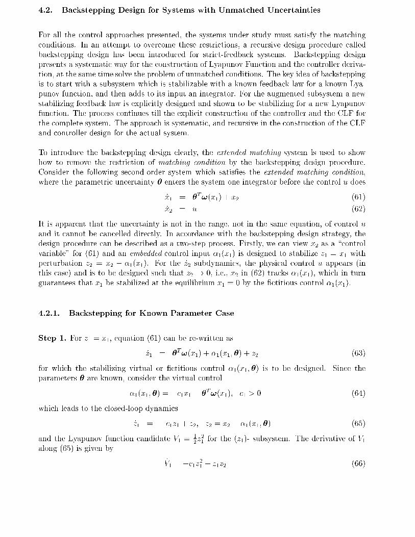
To introduce the backstepping design clearly, the extended matching system is used to show

how to remove the restriction of matching condition by the backstepping design procedure.

Consider the following second-order system which satis�es the extended matching condition,

where the parametric uncertainty � enters the system one integrator before the control u does

_x1 = �T!(x1) + x2 (61)

_x2 = u (62)

It is apparent that the uncertainty is not in the range, not in the same equation, of control u

and it cannot be cancelled directly. In accordance with the backstepping design strategy, the

design procedure can be described as a two-step process. Firstly, we can view x2 as a \control

variable" for (61) and an embedded control input �1(x1) is designed to stabilize z1 = x1 with

perturbation z2 = x2 � �1(x1). For the _z2 subdynamics, the physical control u appears (in

this case) and is to be designed such that z2 ! 0, i.e., x2 in (62) tracks �1(x1), which in turn

guarantees that x1 be stabilized at the equilibrium x1 = 0 by the �ctitious control �1(x1).

4.2.1. Backstepping for Known Parameter Case

Step 1. For z1 = x1, equation (61) can be re-written as

_z1 = �T!(x1) + �1(x1; �) + z2 (63)

for which the stabilizing virtual or �ctitious control �1(x1; �) is to be designed. Since the

parameters � are known, consider the virtual control

�1(x1; �) = �c1x1 � �T!(x1); c1 > 0 (64)

which leads to the closed-loop dynamics

_z1 = �c1z1 + z2; z2 = x2 � �1(x1; �) (65)

and the Lyapunov function candidate V1 =12z21 for the (z1)- subsystem. The derivative of V1

along (65) is given by

_V1 = �c1z21 + z1z2 (66)

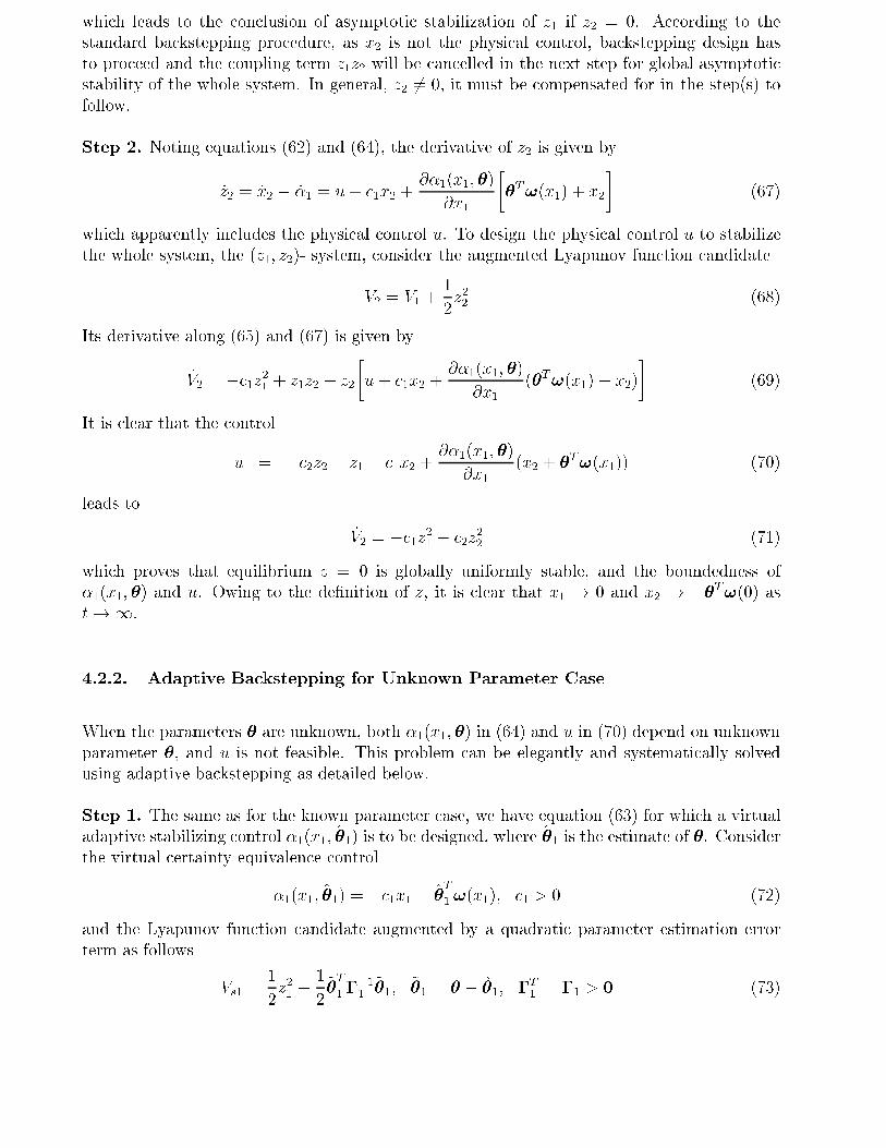
which leads to the conclusion of asymptotic stabilization of z1 if z2 = 0. According to the

standard backstepping procedure, as x2 is not the physical control, backstepping design has

to proceed and the coupling term z1z2 will be cancelled in the next step for global asymptotic

stability of the whole system. In general, z2 6= 0, it must be compensated for in the step(s) to

follow.

Step 2. Noting equations (62) and (64), the derivative of z2 is given by

_z2 = _x2 � _�1 = u+ c1x2 +@�1(x1; �)

@x1

��T!(x1) + x2

�(67)

which apparently includes the physical control u. To design the physical control u to stabilize

the whole system, the (z1; z2)- system, consider the augmented Lyapunov function candidate

V2 = V1 +1

2z22 (68)

Its derivative along (65) and (67) is given by

_V2 = �c1z21 + z1z2 + z2

�u+ c1x2 +

@�1(x1; �)

@x1

(�T!(x1) + x2)

�(69)

It is clear that the control

u = �c2z2 � z1 � c1x2 +@�1(x1; �)

@x1

(x2 + �T!(x1)) (70)

leads to

_V2 = �c1z21 � c2z

22 (71)

which proves that equilibrium z = 0 is globally uniformly stable, and the boundedness of

�1(x1; �) and u. Owing to the de�nition of z, it is clear that x1 ! 0 and x2 ! ��T!(0) ast!1.

4.2.2. Adaptive Backstepping for Unknown Parameter Case

When the parameters � are unknown, both �1(x1; �) in (64) and u in (70) depend on unknown

parameter �, and u is not feasible. This problem can be elegantly and systematically solved

using adaptive backstepping as detailed below.

Step 1. The same as for the known parameter case, we have equation (63) for which a virtual

adaptive stabilizing control �1(x1; �̂1) is to be designed, where �̂1 is the estimate of �. Consider

the virtual certainty equivalence control

�1(x1; �̂1) = �c1x1 � �̂T

1!(x1); c1 > 0 (72)

and the Lyapunov function candidate augmented by a quadratic parameter estimation error

term as follows

Vs1 =1

2z21 +

1

2~�T

1 ��11~�1; ~�1 = � � �̂1; �T

1 = �1 > 0 (73)

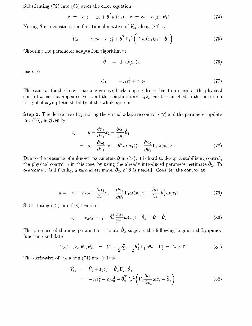
Substituting (72) into (63) gives the error equation

_z1 = �c1z1 + z2 + ~�T

1!(x1); z2 = x2 � �(x1; �̂1) (74)

Noting � is a constant, the �rst time derivative of Vs1 along (74) is

_Vs1 = z1z2 � c1z

21 +

~�T

1��11

��1!(x1)z1 � _̂

�1

�(75)

Choosing the parameter adaptation algorithm as

_̂�1 = �1!(x1)x1 (76)

leads to

_Vs1 = �c1z21 + z1z2 (77)

The same as for the known parameter case, backstepping design has to proceed as the physical

control u has not appeared yet, and the coupling term z1z2 can be cancelled in the next step

for global asymptotic stability of the whole system.

Step 2. The derivative of z2, noting the virtual adaptive control (72) and the parameter update

law (76), is given by

_z2 = u� @�1

@x1

_x1 �@�1

@�̂1

_̂�1

= u� @�1

@x1

(x2 + �T!(x1))�@�1

@�̂1�1!(x1)z1 (78)

Due to the presence of unknown parameters � in (78), it is hard to design a stabilizing control,

the physical control u in this case, by using the already introduced parameter estimate �̂1. To

overcome this diÆculty, a second estimate, �̂2, of � is needed. Consider the control as

u = �z1 � c2z2 +@�1

@x1

x2 +@�1

@�̂1�1!(x1)z1 +

@�1

@x1

�̂T

2!(x1) (79)

Substituting (79) into (78) leads to

_z2 = �c2z2 � z1 � ~�T

2

@�1

@x1

!(x1); ~�2 = � � �̂2 (80)

The presence of the new parameter estimate �̂2 suggests the following augmented Lyapunov

function candidate

Vs2(z1; z2; �̂1; �̂2) = V1 +1

2z22 +

1

2~�T

2��12~�2; �T

2 = �2 > 0 (81)

The derivative of Vs2 along (74) and (80) is

_Vs2 = _

V1 + z2 _z22 � ~�

T

2��12

_̂�2

= �c1z21 � c2z22 � ~�

T

2��12

��2

@�1

@x1

!z2 � _̂�2

�(82)

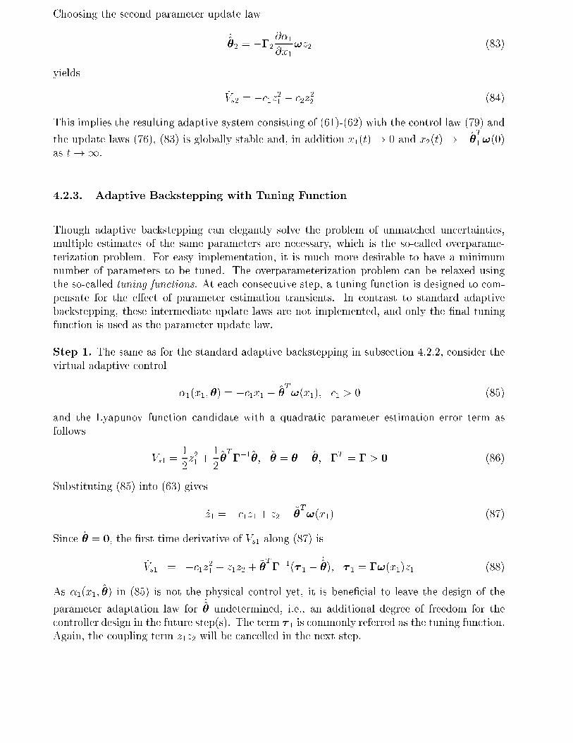
Choosing the second parameter update law

_̂�2 = ��2

@�1

@x1

!z2 (83)

yields

_Vs2 = �c1z21 � c2z

22 (84)

This implies the resulting adaptive system consisting of (61)-(62) with the control law (79) and

the update laws (76), (83) is globally stable and, in addition x1(t)! 0 and x2(t) ! ��̂T1!(0)as t!1.

4.2.3. Adaptive Backstepping with Tuning Function

Though adaptive backstepping can elegantly solve the problem of unmatched uncertainties,

multiple estimates of the same parameters are necessary, which is the so-called overparame-

terization problem. For easy implementation, it is much more desirable to have a minimum

number of parameters to be tuned. The overparameterization problem can be relaxed using

the so-called tuning functions. At each consecutive step, a tuning function is designed to com-

pensate for the e�ect of parameter estimation transients. In contrast to standard adaptive

backstepping, these intermediate update laws are not implemented, and only the �nal tuning

function is used as the parameter update law.

Step 1. The same as for the standard adaptive backstepping in subsection 4.2.2, consider the

virtual adaptive control

�1(x1; �̂) = �c1x1 � �̂T!(x1); c1 > 0 (85)

and the Lyapunov function candidate with a quadratic parameter estimation error term as

follows

Vs1 =1

2z21 +

1

2~�T��1~�; ~� = � � �̂; �T = � > 0 (86)

Substituting (85) into (63) gives

_z1 = �c1z1 + z2 + ~�T!(x1) (87)

Since _� = 0, the �rst time derivative of Vs1 along (87) is

_Vs1 = �c1z21 + z1z2 + ~�

T��1(� 1 � _̂

�); � 1 = �!(x1)z1 (88)

As �1(x1; �̂) in (85) is not the physical control yet, it is bene�cial to leave the design of the

parameter adaptation law for_̂� undetermined, i.e., an additional degree of freedom for the

controller design in the future step(s). The term � 1 is commonly referred as the tuning function.

Again, the coupling term z1z2 will be cancelled in the next step.

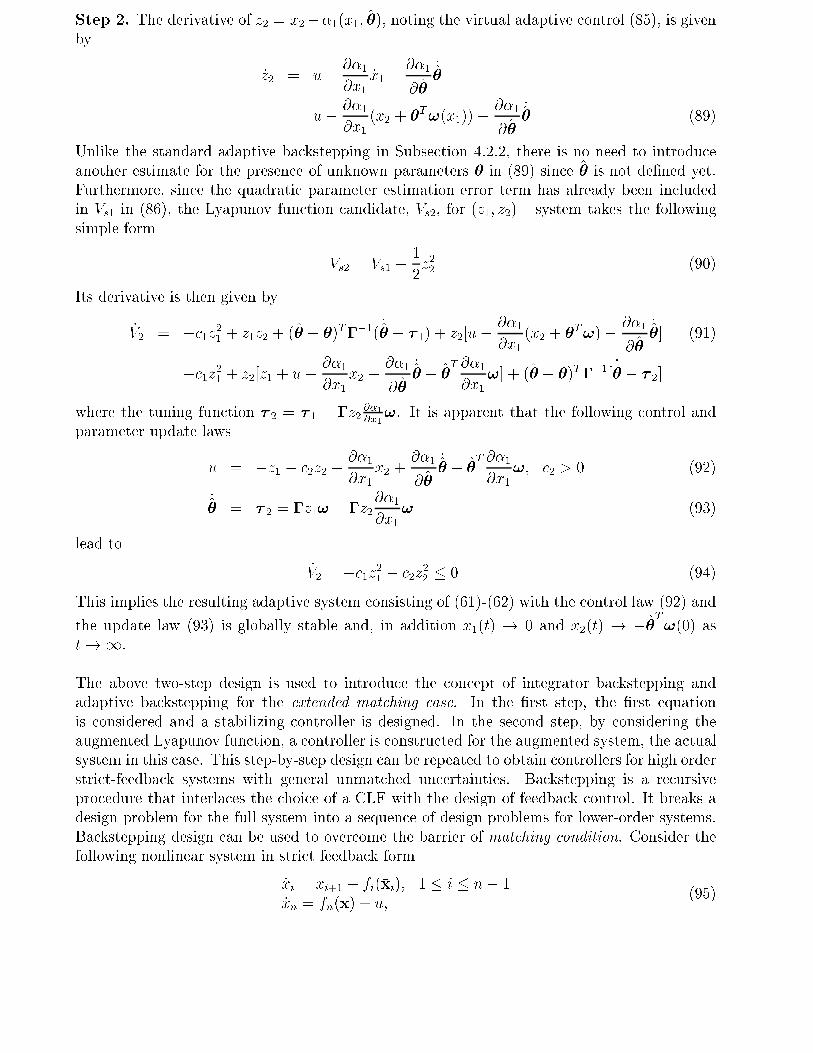
Step 2. The derivative of z2 = x2��1(x1; �̂), noting the virtual adaptive control (85), is given

by

_z2 = u� @�1

@x1

_x1 �@�1

@�̂

_̂�

= u� @�1

@x1

(x2 + �T!(x1))�@�1

@�̂

_̂� (89)

Unlike the standard adaptive backstepping in Subsection 4.2.2, there is no need to introduce

another estimate for the presence of unknown parameters � in (89) since �̂ is not de�ned yet.

Furthermore, since the quadratic parameter estimation error term has already been included

in Vs1 in (86), the Lyapunov function candidate, Vs2, for (z1; z2)� system takes the following

simple form

Vs2 = Vs1 +1

2z22 (90)

Its derivative is then given by

_V2 = �c1z21 + z1z2 + (�̂ � �)T��1(

_̂� � � 1) + z2[u�

@�1

@x1

(x2 + �T!)� @�1

@�̂

_̂�] (91)

= �c1z21 + z2[z1 + u� @�1

@x1

x2 �@�1

@�̂

_̂� � �̂

T @�1

@x1

!] + (�̂ � �)T��1[_̂� � � 2]

where the tuning function � 2 = � 1 � �z2@�1@x1

!. It is apparent that the following control and

parameter update laws

u = �z1 � c2z2 +@�1

@x1

x2 +@�1

@�̂

_̂� + �̂

T @�1

@x1

!; c2 > 0 (92)

_̂� = � 2 = �z1! � �z2

@�1

@x1

! (93)

lead to

_V2 = �c1z21 � c2z

22 � 0 (94)

This implies the resulting adaptive system consisting of (61)-(62) with the control law (92) and

the update law (93) is globally stable and, in addition x1(t) ! 0 and x2(t) ! ��̂T!(0) ast!1.

The above two-step design is used to introduce the concept of integrator backstepping and

adaptive backstepping for the extended matching case. In the �rst step, the �rst equation

is considered and a stabilizing controller is designed. In the second step, by considering the

augmented Lyapunov function, a controller is constructed for the augmented system, the actual

system in this case. This step-by-step design can be repeated to obtain controllers for high order

strict-feedback systems with general unmatched uncertainties. Backstepping is a recursive

procedure that interlaces the choice of a CLF with the design of feedback control. It breaks a

design problem for the full system into a sequence of design problems for lower-order systems.

Backstepping design can be used to overcome the barrier of matching condition. Consider the

following nonlinear system in strict feedback form

_xi = xi+1 + fi(�xi); 1 � i � n� 1

_xn = fn(x) + u;

(95)

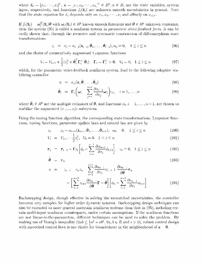
where �xi = [x1; � � � ; xi]T , x = [x1; x2; � � � ; xn]T 2 Rn; u 2 R, are the state variables, system

input, respectively, and functions fi(�xi) are unknown smooth uncertainties in general. Note

that the state equation for _xi depends only on x1; x2; � � � ; xi and aÆnely on xi+1.

If fi(�xi) = !Ti (�xi)� with !i(�xi) 2 R

p known smooth functions and � 2 Rp unknown constants,

then the system (95) is called a nonlinear system in parametric strict-feedback form. It can be

easily shown that, through the recursive and systematic construction of di�eomorphism state

transformations

zi = xi � �i�1(�xi�1; �̂1; : : : ; �̂i�1); �0 = 0; 1 � i � n (96)

and the choice of consecutively augmented Lyapunov functions

Vi = Vi�1 +1

2(z2i +

~�T

i ��1i~�i); �i = �T

i > 0; V0 = 0; 1 � i � n (97)

which, for the parametric strict-feedback nonlinear system, lead to the following adaptive sta-

bilizing controller

u = �n(x; �̂; : : : ; �̂n) (98)

_̂�i = �i

�!i �

i�1Xj=1

@�i�1

@xj

!j

�zi; i = 1; : : : ; n (99)

where �̂i 2 Rp are the multiple estimates of �, and functions �i; i = 1; : : : ; n� 1, are chosen to

stabilize the augmented (z1; :::; zi)- subsystem.

Using the tuning function algorithm, the corresponding state transformations, Lyapunov func-

tions, tuning functions, parameter update laws and control law are given by

zi = xi � �i�1(�xi�1; �̂1; : : : ; �̂i�1); �0 = 0; 1 � i � n (100)

Vi = Vi�1 +1

2z2i ; V0 = 0; 1 � i � n (101)

� i = � i�1 � �zi

��i �

n�1Xi=1

@�n�1

@xi

�i+1

�; �0 = 0; 1 � i � n (102)

_̂� = � n (103)

u = �zn�1 � cnzn +

n�1Xi=1

@�n�1

@xi

xi+1 +@�n�1

@�̂� n

+

� n�2Xi=1

zi+1

@�n�1

@�̂�� �̂

���n �

n�1Xi=1

@�n�1

@xi

�i+1

�(104)

Backstepping design, though e�ective in solving the unmatched uncertainties, the controller

becomes very complex for higher order dynamic systems. Backstepping design techniques can

also be extended to more general uncertain nonlinear systems than that in (95), including cer-

tain multi-input nonlinear counterparts, under certain assumptions. If the nonlinear functions

are not linear-in-the-parameters, di�erent techniques can be used to solve the problem. By

making use of Young's inequality (2ab � 1�a2 + �b

2, 8a; b 2 R and � > 0), robust control design

with smoothed control laws is one choice for boundedness in the neighborhood of z = 0.

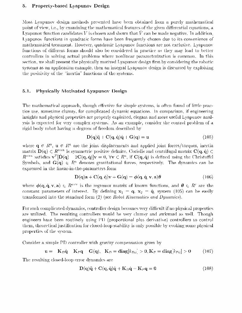
5. Property-based Lyapunov Design

Most Lyapunov design methods presented have been obtained from a purely mathematical

point of view, i.e., by examining the mathematical features of the given di�erential equations, a

Lyapunov function candidates V is chosen and shown that _V can be made negative. In addition,

Lyapunov functions in quadratic forms have been frequently chosen due to its convenience of

mathematical treatment. However, quadratic Lyapunov functions are not exclusive. Lyapunov

functions of di�erent forms should also be considered in practice as they may lead to better

controllers in solving actual problems where nonlinear parameterization is common. In this

section, we shall present the physically motived Lyapunov design �rst by considering the robotic

systems as an application example, then an integral Lyapunov design is discussed by exploiting

the positivity of the \inertia" functions of the systems.

5.1. Physically Motivated Lyapunov Design

The mathematical approach, though e�ective for simple systems, is often found of little prac-

tice use, sometime clumsy, for complicated dynamic equations. In comparison, if engineering

insights and physical properties are properly exploited, elegant and more useful Lyapunov anal-

ysis is expected for very complex systems. As an example, consider the control problem of a

rigid body robot having n degrees of freedom described by

D(q)�q+C(q; _q) _q+G(q) = u (105)

where q 2 Rn, u 2 R

n are the joint displacements and applied joint forces/torques, inertia

matrix D(q) 2 Rn�n is symmetric positive de�nite, Coriolis and centrifugal matrix C(q; _q) 2

Rn�n satis�es vT [ _D(q) � 2C(q; _q)]v = 0, 8v 2 R

n, if C(q; _q) is de�ned using the Christo�el

Symbols, and G(q) 2 Rn denotes gravitational forces, respectively. The dynamics can be

expressed in the linear-in-the-parameters form

D(q)a +C(q; _q)v +G(q) = �(q; _q;v; a)� (106)

where �(q; _q;v; a) 2 Rn�r is the regressor matrix of known functions, and � 2 R

r are the

constant parameters of interest. By de�ning x1 = q, x2 = _q, system (105) can be easily

transformed into the standard form (2) (see Robot Kinematics and Dynamics).

For such complicated dynamics, controller design becomes very diÆcult if no physical properties

are utilized. The resulting controllers would be very clumsy and awkward as well. Though

engineers have been routinely using PD (proportional plus derivative) controllers to control

them, theoretical justi�cation for closed-loop stability is only possible by evoking some physical

properties of the system.

Consider a simple PD controller with gravity compensation given by

u = �KD _q�KPq+G(q); KD = diag[kDii] > 0;KP = diag[kPii] > 0 (107)

The resulting closed-loop error dynamics are

D(q)�q+C(q; _q) _q +KD _q +KPq = 0 (108)

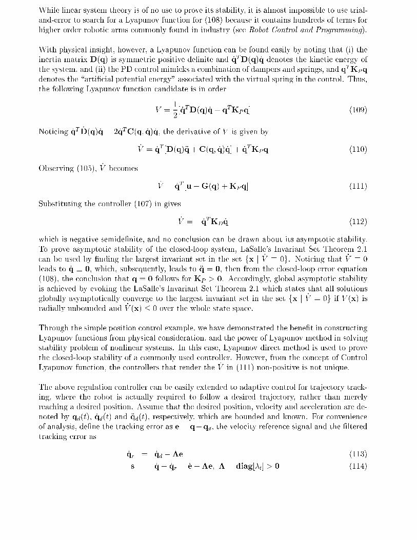
While linear system theory is of no use to prove its stability, it is almost impossible to use trial-

and-error to search for a Lyapunov function for (108) because it contains hundreds of terms for

higher order robotic arms commonly found in industry (see Robot Control and Programming).

With physical insight, however, a Lyapunov function can be found easily by noting that (i) the

inertia matrix D(q) is symmetric positive de�nite and _qTD(q) _q denotes the kinetic energy of

the system, and (ii) the PD control mimicks a combination of dampers and springs, and qTKPq

denotes the \arti�cial potential energy" associated with the virtual spring in the control. Thus,

the following Lyapunov function candidate is in order

V =1

2[ _qTD(q) _q+ qTKPq] (109)

Noticing _qT _D(q) _q = 2 _qTC(q; _q) _q, the derivative of V is given by

_V = _qT [D(q)�q+C(q; _q) _q] + _qTKPq (110)

Observing (105), _V becomes

_V = _qT [u�G(q) +KPq] (111)

Substituting the controller (107) in gives

_V = � _qTKD _q (112)

which is negative semide�nite, and no conclusion can be drawn about its asymptotic stability.

To prove asymptotic stability of the closed-loop system, LaSalle's Invariant Set Theorem 2.1

can be used by �nding the largest invariant set in the set fx j _V � 0g. Noticing that _

V � 0

leads to _q � 0, which, subsequently, leads to �q = 0, then from the closed-loop error equation

(108), the conclusion that q = 0 follows for KP > 0. Accordingly, global asymptotic stability

is achieved by evoking the LaSalle's Invariant Set Theorem 2.1 which states that all solutions

globally asymptotically converge to the largest invariant set in the set fx j _V = 0g if V (x) is

radially unbounded and _V (x) � 0 over the whole state space.

Through the simple position control example, we have demonstrated the bene�t in constructing

Lyapunov functions from physical consideration, and the power of Lyapunov method in solving

stability problem of nonlinear systems. In this case, Lyapunov direct method is used to prove

the closed-loop stability of a commonly used controller. However, from the concept of Control

Lyapunov function, the controllers that render the _V in (111) non-positive is not unique.

The above regulation controller can be easily extended to adaptive control for trajectory track-

ing, where the robot is actually required to follow a desired trajectory, rather than merely

reaching a desired position. Assume that the desired position, velocity and acceleration are de-

noted by qd(t), _qd(t) and �qd(t), respectively, which are bounded and known. For convenience

of analysis, de�ne the tracking error as e = q�qd, the velocity reference signal and the �ltered

tracking error as

_qr = _qd ��e (113)

s = _q� _qr = _e+�e; � = diag[�i] > 0 (114)

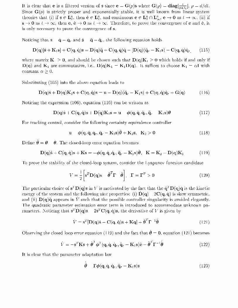
It is clear that e is a �ltered version of s since e = G(p)s where G(p) = diag[ 1p+�i

], p = d=dt.

Since G(p) is strictly proper and exponentially stable, it is well known from linear system

theories that (i) if s 2 Ln2 , then _e 2 Ln

2 , and continuous e 2 Ln2 \ Ln

1, e ! 0 as t !1, (ii) if

s! 0 as t !1, then e, _e! 0 as t !1. Therefore, to prove the convergence of e and _e, it

is only necessary to prove the convergence of s.

Noticing that s = _q� _qr and _s = �q� �qr, the following equation holds

D(q)[ _s+K1s] +C(q; _q)s = D(q)�q+C(q; _q) _q� [D(q)(�qr �K1s) +C(q; _q) _qr] (115)

where matrix K1 � 0, and should be chosen such that D(q)K1 � 0 which holds if and only if

D(q) and K1 are commutative, i.e., D(q)K1 = K1D(q). It suÆces to choose K1 = �I with

constant � � 0.

Substituting (105) into the above equation leads to

D(q)_s+D(q)K1s +C(q; _q)s = u�D(q)(�qr �K1s) +C(q; _q) _qr +G(q) (116)

Noticing the expression (106), equation (116) can be written as

D(q)_s+C(q; _q)s+D(q)K1s = u� �(q; _q; _qr; �qr �K1s)� (117)

For tracking control, consider the following certainty equivalence controller

u = �(q; _q; _qr; �qr �K1s)�̂ +K2s; K2 > 0 (118)

De�ne ~� = � � �̂. The closed-loop error equation becomes

D(q)_s+C(q; _q)s+Ks = ��(q; _q; _qr; �qr �K1s)~�; K = K2 +D(q)K1 (119)

To prove the stability of the closed-loop system, consider the Lyapunov function candidate

V =1

2

�sTD(q)s+ ~�

T��1~�

�; � = �T

> 0 (120)

The particular choice of sTD(q)s in V is motivated by the fact that the _qTD(q) _q is the kinetic

energy of the system and the following nice properties: (i) _D(q)� 2C(q; _q) is skew symmetric,

and (ii) D(q)�q appears in _V such that the possible controller singularity is avoided elegantly.

The quadratic parameter estimation error term is introduced to accommodate unknown pa-

rameters. Noticing that sT _D(q)s = 2sTC(q; _q)s, the derivative of V is given by

_V = sT [D(q)_s +C(q; _q)s+Kq] + ~�

T��1

_~� (121)

Observing the closed-loop error equation (119) and the fact that _� = 0, equation (121) becomes

_V = �sTKs+ ~�

T�T (q; _q; _qr; �qr �K1s) _e+ ~�

T��1

_̂� (122)

It is clear that the parameter adaptation law

_̂� = ��(q; _q; _qr; �qr �K1s)s (123)

renders

_V = �sTKs (124)

which leads to the following two inequalities

�V (0) � V (t)� V (0) =

Z t

0

_V (�)d� = �

Z t

0

sTKsd�

Z t

0

ks(�)k2d� � V (0)

�max(K)<1

Accordingly, we have s 2 L2, _e 2 Ln2 and continous e! 0 as t!1. The boundedness of s and

~� follow directly from the boundedness of V . The boundedness of �̂ is obtainable by noticing

that � is constant. From (119), it is clear that _s is bounded. The combination of s 2 L2 and

bounded _s leads to s! 0 as t!1, which subsequently leads to limt!1 e = 0.

It is clear that with the di�erent choice of Lyapunov function, there is no need to invoke the

invariant set theorem for the conclusion of asymptotic stability.

5.2. Integral Lyapunov Function for Nonlinear Parameterizations

Lyapunov functions in quadratic form have been frequently chosen due to their convenience of

mathematical treatment. In practice, other forms should also be considered, and in some cases,

they may lead to better controllers in solving actual problems where nonlinear parameterization

is common. In this section, an integral Lyapunov function is presented, which results in a con-

troller structure that avoids the possible controller singularity problem encountered in feedback

linearization completely without evoking any preventing measures such as the so-called ��modi�cation, projection algorithms, and among others. For simplicity, consider the following

simple nonlinear system as it can be easily generalized

m(x) _x = f(x) + u (125)

where x 2 R, u 2 R, y 2 R are the state variable, system input and output, respectively;

continuous functions m(x) > 0 and f(x) can be expressed as

m(x) = �T!m(x); f(x) = �T!f (x) (126)

where � 2 Rp is a vector of unknown constant parameters, !m(x) 2 R

p and !f (x) 2 Rp are

known regressor vectors.

The objective is to control x to follow a given reference signal yd. De�ne e = x � yd. From

(125), the time derivative of e can be written as

m(x) _e = f(x) + u�m(x) _yd (127)

Let m�(x) = m(x)�(x) where �(x): R ! R+ is a smooth weighting function, and is used for

appropriate choice of integral functions to be introduced. Noting that x = e + yd, for ease of

discussion, denote m�(e+ yd) = m�(x).

De�ne the integral Lyapunov function candidate as

V0 =

Z e

0

�m�(� + yd)d� (128)

which is made radially unbounded by choosing appropriate �(x).

The time derivative of V0 given in (128) is

_V0 = em�(x) _e + _yd

Z e

0

�

@m�(� + yd)

@yd

d�

= em�(x) _e + _yd

Z e

0

�

@m�(� + yd)

@�

d�

= e�(x)m(x) _e + _ydm�(x)e + _yd

Z e

0

m�(� + yd)d� (129)

Substituting (127) into (129) leads to

_V0 = e�(x)

�f(x) + u+

_yd

e�(x)

Z e

0

m�(� + yd)d�

�(130)

Noting the expressions in (126), equation (130) becomes

_V0 = e�(x)[�T!(z) + u] (131)

where

!(z) = !f (x) +_yd

e�(x)

Z e

0

!m(� + yd)�(� + yd)d�; z = [x; yd; _yd]T 2 R

3 (132)

It can be checked that

lime!0

!(z) = !f(x) +_yd!m(yd)�(yd)

�(x)(133)

which means that !(z) is well de�ned. If the parameter vector � is available, a possible

controller is u = [� ke

�(x)� �T!(z)] with design parameter k > 0. For this controller, (131)

becomes _V0 = �ke2 < 0; 8e 6= 0. According to De�nition 2.2, we conclude that V0 is a CLF

and e! 0 as t!1.

In the case of unknown parameter �, consider its certainty-equivalence controller given by

u =

�� ke

�(x)� �̂

T!(z)

�(134)

where �̂ is the estimate of �. Substituting (134) into (131) leads to

_V0 = �ke2 + ~�

T!(z)�(x)e; ~� = � � �̂ (135)

The system stability is not clear at this stage yet because the last term in (135) is inde�nite

and contains unknown ~�. To remove such an uncertain term with ~�, consider the following

augmented Lyapunov function candidate

V = V0 +1

2~�T��1~�; � = �T

> 0 (136)

Its time derivative is

_V = �e2 + ~�

T��1

h�!(z)�(x)e+

_̂�i

(137)

The following adaptive law

_̂� = �!(z)�(x)e (138)

leads to

_V = �ke2 � 0 (139)

This guarantees that V (0) 2 L1 for any bounded initial values x(0) and yd(0). Integrating

(139), we haveR1

0e2(�)d� � V (0) <1 and 0 � V (t) � V (0). This implies that e 2 L2 \ L1

and �̂(t) is bounded. Consequently, u and _e are also bounded. Since e 2 L2 \ L1 and _e 2 L1,

we conclude limt!1 e = 0 by Barbalat's Lemma 2.1.

Di�erent choices of weighting function �(x) may produce di�erent control performance. For

m�(x) = �T!m(x)�(x) with known functions !m(x), it is not diÆcult to design �(x) such that

0 < c1 � m�(x) � c0. For example, if m(x) = exp(�x2)(�1 + �2x2) with constant parameters

�1; �2 > 0, then one may take �(x) = exp(x2)=(1 + x2) which leads to

min(�1; �2) � m�(x) =�1 + �2x

2

1 + x2

� max(�1; �2)

Though the concepts are introduced through a simple �rst order system, it can be applied to

a larger class of the system of the form directly

_xi = xi+1 ; i = 1; 2; � � � ; n� 1

_xn =f(x)

m(x)+

1

m(x)u

(140)

where x = [x1 x2 � � � xn]T 2 R

n, u 2 R, are the state variables, and input, respectively,

functions f(x); m(x) may take the following forms

f(x) = �T!f(x) + f0(x); m(x) = �T!m(x) +m0(x) > 0 (141)

where � 2 Rp is a vector of unknown constant parameters, !f(x) 2 R

p and !m(x) 2 Rp are

known regressor vectors, continuous functions f0(x) and m0(x) are known.

Furthermore, by combining function approximation, adaptive backstepping control design using

the integral Lyapunov functions, semi-globally stable and singularity-free adaptive controller

can be obtained for the following class of nonlinear systems in strict-feedback form

�_xi = fi(�xi) + gi(�xi)xi+1; 1 � i � n� 1

_xn = fn(x) + gn(x)u(142)

where �xi = [x1; � � � ; xi]T , x = [x1; x2; � � � ; xn]T 2 Rn; u 2 R are the state variables, and system

input, respectively; fi(�) and gi(�) > 0; i = 1; 2; � � � ; n are unknown smooth functions and may

not be linearly parameterized. It can also be applied to the following MIMO nonlinear system

where the inputs appear in a triangular manner as follows

8>>>>>>>>><>>>>>>>>>:

_x1;i1 = x1;i1+1

_x1;�1 = f1(X) + g1;1(x1)u1_x2;i2 = x2;i2+1

_x2;�2 = f2(X; u1) + g2;2(x1; x2)u2...

_xj;ij = xj;ij+1

_xj;�j = fj(X; u1; � � � ; uj�1) + gj;j(x1; x2; � � � ; xj)uj

(143)

where X = [xT1 ;xT2 ; � � � ;xTm]T with xj = [xj;1; xj;2; � � � ; xj;�j ]T 2 R

�j and uj 2 R are the state

variables, the system inputs, respectively; fj(�) and gj;i(�) are unknown smooth functions; �j,

m, 1 � j � m and 1 � ij � �j � 1 are positive integers de�ning the order and the complexity

of the system.

6. Design Flexibilities and Considerations

Except for the MRAC Lyapunov design where the selection of Lyapunov functions and control

laws are systematic and straightforward, the degrees of freedom in Lyapunov design in general

are numerous, case dependent, and allow for the careful shaping of the closed-loop performance.

Though MRAC can specify the desired performance elegantly, it is in essence a feedback lin-

earization design, in which it tries to replace all the linear/nonlinear terms indiscriminately of

the system by the desired linear terms for closed-loop stability (see Feedback Linearization).

As a results, some stabilizing nonlinearities are also been canceled by the control law. As an

example, consider the stabilization problem of the following scalar dynamic system

_x = 2 cos(x)� x3 + u (144)

Following the technique of feedback linearization, and taking Am = 1, the following control is

in order

u = �2 cos(x) + x3 � x (145)

The stability can be seen by taking Q = 1 (corresponding to W (x) = x2) and solve (26) for

P = 1=2 which corresponds to Lyapunov function V (x) = x2=2.

The control law (145) indiscriminately cancels both nonlinearities cos x and �x3 altogether,

and replaces them with �x such that the resulting feedback system is a stable linear system,

_x = �x. Though stability is guaranteed with the automatic construction of the controller,

it is obviously irrational to cancel �x3 without further analysis. For stabilization at x = 0,

the negative feedback term �x3 is helpful, especially when x is large. At the same time, the

presence of x3 in the control law (145) is harmful. It leads to a large magnitude of control u

that may cause many practical problems. It would be more reasonable to selectively cancel the

nonlinearities. Consider V (x) = 12x2 as before. Its derivative is

_V = x(2 cos(x)� x

3 + u) = �x4 + x(2 cos(x)� u) (146)

It is clear that there is no need to cancel the �x3 term at all as it is stabilizing. Choosing

u = �2 cos(x) � x which grows only linearly with x leads to _V = �W (x) � 0 where W (x) =

x2 + x

4.

As said earlier, Lyapunov design is not unique and problem dependent. Another control law

can be obtained via universal control (7). Since it is based on the assumption that f(0) = 0,

the system needs to be converted into the required form �rst. Consider u = �2 cos(x) + v

where v is a new control to be de�ned, the system is transformed into _x = �x3 + v. Again,

considering V (x) = 12x2 as the CLF with f(x) = �x3 and g(x) = 1, the universal control v is

given by

v = x3 � x

px4 + 1 (147)

A very nice property of (147) is that v ! 0 as jxj ! 1, which means that for large jxj thecontrol law for u reduces to the term � cos x required to place the equilibrium at x = 0. It is

easy to check that u = � cos x + v satis�es (5) with W (x) = x2px4 + 1. This control law is

superior because it requires less control e�ort than the other two.

From the simple example, it is clear that the choices for functions �i in the iterative back-

stepping design are by no means unique, nor is the �nal choice for the control law. In a more

general setting, it is hard to choose the intermediate control �i. In actual applications, it is

problem dependent. From a theoretical point of view, optimal control or sub-optimal control

may be considered according to some meaningful cost functions. At each step, wasteful cancel-

lations of the bene�cial nonlinearities can be avoided. However, the reasonable and bene�cial

intermediate-step controls, especially at the earlier steps, may not be proven bene�cial for the

�nal design for the physical system. Further research is needed.

The choices for Vi are not unique as have been demonstrated in the article earlier. Recall that

given a Lyapunov function Vi and control �i at the ith design step, the new Lyapunov function

Vi+1 is given by

Vi = Vi�1 +1

2z2i (148)

This choice for Vi+1 is not the only choice that will lead to a successful design. Another degree

of freedom is available in the design procedure. In this article, several types of Lyapunov

functions, quadratic, energy-based quadratic and integral, have been presented, and they can

be blended together in actual controller design for the best result. For example, at one step, one

type of Lyapunov functions can be used, at the next step, another type can be considered by

examining the properties of the system. Note that the types of Lyapunov functions introduced

in the article are by no means exclusive. Numerous other types and di�erent variations can be

explored. It has been shown that 12z2i can be replaced by the general expression

Z xi+1

�i

�(�xi; s)ds

for a suitable choice of the function �. The former is a special case of the latter for � = s��i(�xi).

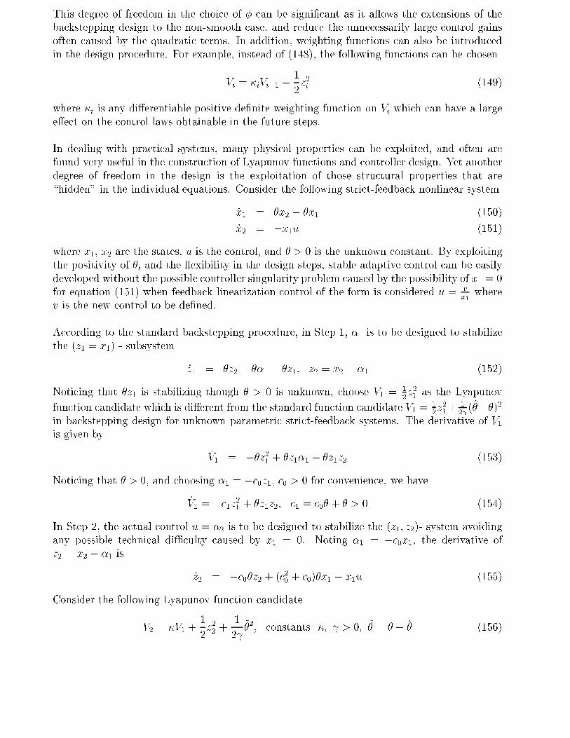
This degree of freedom in the choice of � can be signi�cant as it allows the extensions of the

backstepping design to the non-smooth case, and reduce the unnecessarily large control gains

often caused by the quadratic terms. In addition, weighting functions can also be introduced

in the design procedure. For example, instead of (148), the following functions can be chosen

Vi = �iVi�1 +1

2z2i (149)

where �i is any di�erentiable positive de�nite weighting function on Vi which can have a large

e�ect on the control laws obtainable in the future steps.

In dealing with practical systems, many physical properties can be exploited, and often are

found very useful in the construction of Lyapunov functions and controller design. Yet another

degree of freedom in the design is the exploitation of those structural properties that are

\hidden" in the individual equations. Consider the following strict-feedback nonlinear system

_x1 = �x2 � �x1 (150)

_x2 = �x1u (151)

where x1, x2 are the states, u is the control, and � > 0 is the unknown constant. By exploiting

the positivity of �, and the exibility in the design steps, stable adaptive control can be easily

developed without the possible controller singularity problem caused by the possibility of x1 = 0

for equation (151) when feedback linearization control of the form is considered u = v

x1where

v is the new control to be de�ned.

According to the standard backstepping procedure, in Step 1, �1 is to be designed to stabilize

the (z1 = x1) - subsystem

_z1 = �z2 + ��1 � �z1; z2 = x2 � �1 (152)

Noticing that �z1 is stabilizing though � > 0 is unknown, choose V1 =12z21 as the Lyapunov

function candidate which is di�erent from the standard function candidate V1 =12z21+

12 (�̂��)2

in backstepping design for unknown parametric strict-feedback systems. The derivative of V1is given by

_V1 = ��z21 + �z1�1 + �z1z2 (153)

Noticing that � > 0, and choosing �1 = �c0z1, c0 > 0 for convenience, we have

_V1 = �c1z21 + �z1z2; c1 = c0� + � > 0 (154)

In Step 2, the actual control u = �2 is to be designed to stabilize the (z1; z2)- system avoiding

any possible technical diÆculty caused by x1 = 0. Noting �1 = �c0x1, the derivative of

z2 = x2 � �1 is

_z2 = �c0�z2 + (c20 + c0)�x1 � x1u (155)

Consider the following Lyapunov function candidate

V2 = �V1 +1

2z22 +

1

2 ~�2; constants �; > 0; ~

� = � � �̂ (156)

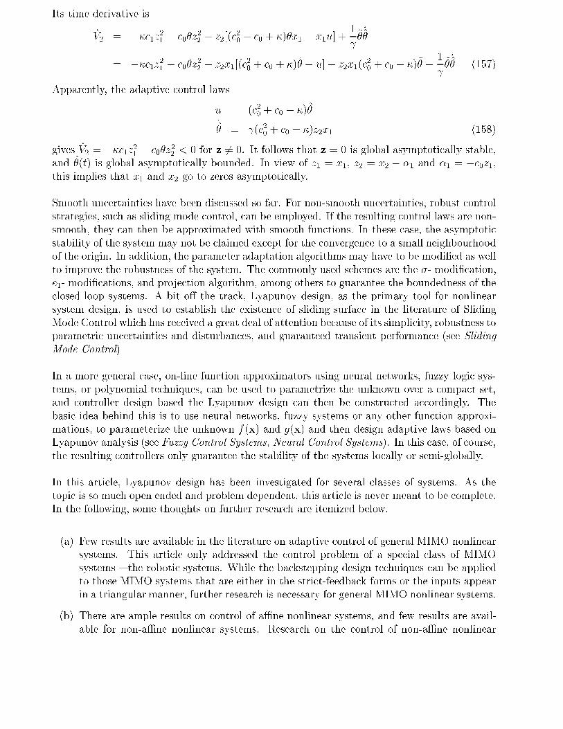
Its time derivative is

_V2 = ��c1z21 � c0�z

22 + z2[(c

20 + c0 + �)�x1 � x1u] +

1

~�

_~�

= ��c1z21 � c0�z22 + z2x1[(c

20 + c0 + �)�̂ � u] + z2x1(c

20 + c0 + �)~� � 1

~�

_̂� (157)

Apparently, the adaptive control laws

u = (c20 + c0 + �)�̂

_̂� = (c20 + c0 + �)z2x1 (158)

gives _V2 = ��c1z21 � c0�z

22 < 0 for z 6= 0. It follows that z = 0 is global asymptotically stable,

and �̂(t) is global asymptotically bounded. In view of z1 = x1, z2 = x2 � �1 and �1 = �c0z1,this implies that x1 and x2 go to zeros asymptotically.

Smooth uncertainties have been discussed so far. For non-smooth uncertainties, robust control

strategies, such as sliding mode control, can be employed. If the resulting control laws are non-

smooth, they can then be approximated with smooth functions. In these case, the asymptotic

stability of the system may not be claimed except for the convergence to a small neighbourhood

of the origin. In addition, the parameter adaptation algorithms may have to be modi�ed as well

to improve the robustness of the system. The commonly used schemes are the �- modi�cation,

e1- modi�cations, and projection algorithm, among others to guarantee the boundedness of the

closed-loop systems. A bit o� the track, Lyapunov design, as the primary tool for nonlinear

system design, is used to establish the existence of sliding surface in the literature of Sliding

Mode Control which has received a great deal of attention because of its simplicity, robustness to

parametric uncertainties and disturbances, and guaranteed transient performance (see Sliding

Mode Control)

In a more general case, on-line function approximators using neural networks, fuzzy logic sys-

tems, or polynomial techniques, can be used to parametrize the unknown over a compact set,

and controller design based the Lyapunov design can then be constructed accordingly. The

basic idea behind this is to use neural networks, fuzzy systems or any other function approxi-

mations, to parameterize the unknown f(x) and g(x) and then design adaptive laws based on

Lyapunov analysis (see Fuzzy Control Systems, Neural Control Systems). In this case, of course,

the resulting controllers only guarantee the stability of the systems locally or semi-globally.

In this article, Lyapunov design has been investigated for several classes of systems. As the

topic is so much open ended and problem dependent, this article is never meant to be complete.

In the following, some thoughts on further research are itemized below.

(a) Few results are available in the literature on adaptive control of general MIMO nonlinear

systems. This article only addressed the control problem of a special class of MIMO

systems { the robotic systems. While the backstepping design techniques can be applied

to those MIMO systems that are either in the strict-feedback forms or the inputs appear

in a triangular manner, further research is necessary for general MIMO nonlinear systems.

(b) There are ample results on control of aÆne nonlinear systems, and few results are avail-

able for non-aÆne nonlinear systems. Research on the control of non-aÆne nonlinear

system based on Lyapunov design is an important and challenging problem in further

investigation.

(c) All the elegant methods for continuous-time nonlinear systems in strict-feedback form are

not directly applicable to discrete-time systems in strict-feedback form. Currently only

preliminary results are available, and further results are necessary for controller design of

discrete-time nonlinear systems with general unmatched nonlinearities.

(d) Hybrid dynamical systems that contain both discrete and continuous signals are very

common in reality. Further research on Lyapunov design is also calling attention.

It is believed that pursuing di�erent ways to utilize the structure properties of di�erent systems

would be bene�cial in deriving stable control schemes for a large class of multivariable nonlinear

systems.

7. Conclusions

In this article, an overview has been given on some state-of-the-art approaches of Lyapunov

design, though in general there is no systematic procedure in choosing a suitable Lyapunov

function candidate for controller design for a given nonlinear system. After a brief introduction

and historic review, this article presented (i) the basic concepts of Lyapunov stability and

control Lyapunov functions, (ii) Lyapunov equations and model reference adaptive control

based on Lyapunov design for matched systems, (iii) Lyapunov redesign, adaptive redesign and

robust design for matched systems, (iv) adaptive backstepping design for unmatched nonlinear

systems, (v) Lyapunov design by exploiting physical properties for special classes of systems,

and (vi) design exibilities and considerations in actual design.

Acknowledgements

The author is grateful to H. Unbehauen for the opportunity to contribute to the EOLSS and

to M. Krstic, F.L. Lewis, I.M.Y. Mareels and M.W. Spong for their helpful suggestions in the

preparation of the manuscript.

Bibliography

Astrom K. J. and Wittenmark B. (1995). Adaptive Control, 2nd Edition, Addison-Wesley

Publishing Company. [This is a widely used textbook on adaptive control, which gives the

history development and all the essentials of adaptive control]

Ge S.S., Lee T.H. and Harris C.J. (1998). Adaptive Neural Network Control of Robotic Manip-

ulators, World Scienti�c, London. [This books treats adaptive neural network control of robots

systematically and rigorously using Lyapunov design]

Ge S. S. , Hang C.C. , Lee T.H. and Zhang T. (2001). Stable adaptive Neural Network Control,

Kluwer Academic Publishers, Norwell, USA. [This book deals with neural network control for

some general classes of nonlinear systems and proves closed-loop stability rigorously]

Levine W.S. (Ed.) (1996). The Control handbook, CRC Press, Boca Raton, FL, 1996. [This

book is a very complete introductory reference]

Ioannou P. A. and Sun J. (1996). Robust Adaptive Control, Prentice Hall, New Jersey. [This is a

self-contained tutorial book that uni�es, simpli�es, and presents most of the existing techniques

in designing and analyzing model reference adaptive control systems]

Khalil H. K. (1996). Nonlinear Systems, 2nd Edition, Prentice Hall, New Jersey. [This reference

book is covers all the essential theories on stability, Lyapunov design, nonlinear control, and

backstepping design]

Krstic M., Kanellakopoulos I. and Kokotovic P. (1985), Nonlinear and Adaptive Control De-

sign, John Wiley & Sons, Inc., New York. [This book gives a systematic and comprehensive

treatments of backstepping design and its applications]

Lewis F.L., Abdallah C.T. and Dawson D.M. (1993). Control of Robot Manipulators, Maxwell

Macmillan International, 1993. [This book gives a comrehensive treatment of dynamics and

their properties, and di�erent control techniques]

Marino R. and Tomei P. (1995). Nonlinear Control Design: Geometric, Adaptive and Robust,

Prentice Hall, Englewood Cli�s, New Jersey. [This book gives a systematic treatment of control

system design based on di�erential geometry]

Narendra K.S. and Annaswamy A.M. (1989). Stable Adaptive Control, Prentice Hall, Engle-

wood Cli�s, New Jersey. [This book provides a systematic treatment of model reference adaptive

control]

Qu Z. (1998). Robust Control of Nonlinear Uncertain Systems, John Wiley & Sons, New York.

[This book provides a comprehensive treatment of robust control based on Lyapunov design]

Slotine J. J. E. and Li W. (1991). Applied Nonlinear Control, Prentice Hall, New Jersey. [This

book is a widely used text book on applied nonlinear control, the essential concepts of stability

and controller design are presented elegantly and easy to understand]

Spong M.W. and Vidyasagar M. (1989). Robot Dynamics and Control, John Wiley & Sons,

New York, 1989. [This book provides the essential concepts of robot dynamics and fundmental

tools and theories on robot control]