Embed Size (px)
Citation preview
LUÍS MANUEL TREMOCEIRO BAPTISTA Mestre em Engenharia Electrotécnica e de Computadores
USING RESTARTS IN CONSTRAINT PROGRAMMING OVER FINITE DOMAINS
AN EXPERIMENTAL EVALUATION
Dissertação para obtenção do Grau de Doutor em Informática
Orientador: Francisco de Moura e Castro Ascensão de Azevedo, Professor Auxiliar da Faculdade de Ciências e Tecnologia da Universidade NOVA de Lisboa
Júri
Presidente: Prof. Doutor Pedro Manuel Corrêa Calvente Barahona Arguentes: Prof. Doutor Christophe Lecoutre Prof. Doutor Mikoláš Janota Vogais: Prof. Doutora Ana Paula Tomás Prof. Doutor Francisco de Moura e Castro Ascensão de Azevedo Prof. Doutor José Carlos Ferreira Rodrigues da Cruz Doutor Marco Vargas Correia
Setembro 2017

iii
Using Restarts in Constraint Programming over Finite Domains - An Experimental
Evaluation
Copyright © Luís Manuel Tremoceiro Baptista, Faculdade de Ciências e Tecnologia,
Universidade Nova de Lisboa
A Faculdade de Ciências e Tecnologia e a Universidade Nova de Lisboa têm o
direito, perpétuo e sem limites geográficos, de arquivar e publicar esta dissertação através
de exemplares impressos reproduzidos em papel ou de forma digital, ou por qualquer
outro meio conhecido ou que venha a ser inventado, e de a divulgar através de
repositórios científicos e de admitir a sua cópia e distribuição com objectivos
educacionais ou de investigação, não comerciais, desde que seja dado crédito ao autor e
editor.


v
ACKNOWLEDGEMENTS
To my supervisor, Professor Francisco Azevedo, for the valuable support and
perseverance, especially when good results did not appear. I am thankful that he managed
to find the necessary funding that allowed me to attend important conferences. And also,
to participate in a summer school, where I was introduced and trained with the Comet
System, which I used in this PhD Thesis. I also thank Marco Correia for explaining how
the CaSPER Constraint Solver works, although I have not used it.
To my School of Technology and Business Studies of the Polytechnic Institute of
Portalegre, which gave me all the possible support, among the fewer available.
Particularly, I want to thank to my colleague and friend Paulo Brito for all the support and
encouragement. Also, the work presented in this Thesis was partially supported by the
Portuguese “Fundação para a Ciência e a Tecnologia” (SFRH/PROTEC/49859/2009).
Finally, and most important, I am deeply thankful to all my family for all the support.
Especially to my wife Carla, my son Miguel and my daughter Leonor, for waiting so
patiently that I finish my Thesis, and to whom I took so much family time – this Thesis is
dedicated to them, with love.

vii
ABSTRACT
The use of restart techniques in complete Satisfiability (SAT) algorithms has made
solving hard real world instances possible. Without restarts such algorithms could not
solve those instances, in practice. State of the art algorithms for SAT use restart
techniques, conflict clause recording (nogoods), heuristics based on activity variable in
conflict clauses, among others. Algorithms for SAT and Constraint problems share many
techniques; however, the use of restart techniques in constraint programming with finite
domains (CP(FD)) is not widely used as it is in SAT. We believe that the use of restarts in
CP(FD) algorithms could also be the key to efficiently solve hard combinatorial
problems.
In this PhD thesis we study restarts and associated techniques in CP(FD) solvers. In
particular, we propose to including in a CP(FD) solver restarts, nogoods and heuristics
based in nogoods as this should improve search algorithms, and, consequently, efficiently
solve hard combinatorial problems.
We thus intend to: a) implement restart techniques (successfully used in SAT) to
solve constraint problems with finite domains; b) implement nogoods (learning) and
heuristics based on nogoods, already in use in SAT and associated with restarts; and c)
evaluate the use of restarts and the interplay with the other implemented techniques.
We have conducted the study in the context of domain splitting backtrack search
algorithms with restarts. We have defined domain splitting nogoods that are extracted
from the last branch of the search algorithm before the restart. And, inspired by SAT
solvers, we were able to use information within those nogoods to successfully help the
variable selection heuristics. A frequent restart strategy is also necessary, since our
approach learns from restarts.
Keywords: restarts; nogoods; heuristics; constraint programming; backtrack search.

ix
RESUMO
A utilização de técnicas de restarts em algoritmos completos para Solvabilidade
Proposicional (SAT) tornou possível a resolução de problemas reais difíceis, que na
prática não conseguiam ser resolvidos sem restarts. Os melhores algoritmos de SAT
usam técnicas de restarts, registo de cláusulas de conflito (nogoods), heurísticas baseadas
na atividade de variáveis nas cláusulas de conflito, entre outras técnicas. Os algoritmos
para SAT e para programação por restrições sobre domínios finitos (CP(FD)) partilham
muitas técnicas; no entanto, em CP(FD) os restarts não são usados de forma tão alargado
como em SAT. Pensamos que a utilização de restarts em algoritmos para CP(FD) pode
também ser a chave para resolver de forma mais eficiente problema combinatórios
difíceis.
Nesta tese de doutoramento estudamos em CP(FD) os restarts e técnicas associadas.
Em particular, propomos implementar os restarts, nogoods e heurísticas baseadas em
nogood, de forma a melhorar o algoritmo de procura e, consequentemente, resolver de
forma eficiente problemas combinatórios difíceis.
Assim, pretendemos: a) implementar técnicas de restarts (utilizadas com sucesso em
SAT) para resolver problemas de restrições sobre domínios finitos; b) implementar
nogoods (aprendizagem automática) e heurísticas baseadas nesses nogoods, já utilizadas
em SAT e associadas a restarts; e c) avaliar o uso de restarts e a sua interação com outras
técnicas implementadas.
Este estudo foi levado a cabo no contexto dos algoritmos de procura com retrocesso,
utilizando restarts, e com domain splitting (ds). Definimos nogoods que são extraídos do
último ramo da árvore de procura antes do restart. Inspirados pelos algoritmos de SAT,
conseguimos usar informação contida nos nogoods para ajudar a heurística de seleção de
variável. É necessário uma política de restarts frequentes, uma vez que a nossa
abordagem aprende com os restarts.
Palavras-chave: restarts; nogoods; heurísticas; Programação por restrições; procura
com retrocesso.

x
xi
CONTENTS
1 Introduction ................................................................................................................. 1
1.1 General Overview ............................................................................................... 1
1.2 Challenges and Contributions ............................................................................. 2
1.3 Thesis Map .......................................................................................................... 5
2 Constraint Solving ...................................................................................................... 7
2.1 Constraint Satisfaction Problem .......................................................................... 7
2.1.1 Definitions ................................................................................................... 7
2.1.2 Search algorithms ........................................................................................ 9
2.1.3 Branching schemes ................................................................................... 11
2.1.4 Learning .................................................................................................... 12
2.1.5 Examples of CSP Problems ...................................................................... 14
2.2 Satisfiability Problems ...................................................................................... 23
2.2.1 Definition .................................................................................................. 23
2.2.2 Search Algorithms..................................................................................... 25
2.3 Summary and Final Remarks ............................................................................ 28
3 Heuristics .................................................................................................................. 29
3.1 Static versus dynamic variable ordering heuristics ........................................... 30
3.2 The fail first principle ....................................................................................... 31
3.3 Weighted based (Conflict-driven) heuristic ...................................................... 34
3.4 Other state of the art heuristics ......................................................................... 36
3.5 Sat heuristics ..................................................................................................... 38
3.5.1 The vsids heuristic .................................................................................... 39
CONTENTS
xii
3.6 Summary and Final Remarks ............................................................................ 40
4 Restarts ...................................................................................................................... 43
4.1 Randomization and Heavy-tail .......................................................................... 45
4.2 Search restart strategies ..................................................................................... 47
4.3 Completeness .................................................................................................... 49
4.4 Learning from restarts ....................................................................................... 50
4.5 Results on Restarts ............................................................................................ 53
4.5.1 Preliminary results ..................................................................................... 53
4.5.2 Using Restarts ........................................................................................... 57
4.5.3 Difficulties on using restarts ..................................................................... 61
4.6 Summary and Final Remarks ............................................................................ 62
5 Domain-Splitting Nogoods ....................................................................................... 65
5.1 Simplifying ds-nogoods .................................................................................... 68
5.2 Generalizing to dsg-nogoods ............................................................................. 70
5.3 Posting ds-nogoods ........................................................................................... 71
5.4 Summary and Final Remarks ............................................................................ 76
6 Using Ds-Nogoods in Heuristics ............................................................................... 79
6.1 Trying information from ds-nogoods ................................................................ 81
6.2 Ds-nogood-based heuristic ................................................................................ 85
6.3 Results on ds-nogood based heuristic ............................................................... 87
6.3.1 Talisman squares ....................................................................................... 89
6.3.2 Latin Squares ............................................................................................. 90
6.3.3 Restart strategies ....................................................................................... 91
6.4 Refining the search algorithm ........................................................................... 93
CONTENTS
xiii
6.4.1 Flexible Domain-splitting branching ........................................................ 96
6.4.2 Importance of domain-splitting branching .............................................. 102
6.5 Comparing with dom/wdeg ............................................................................. 104
6.5.1 Importance of domain splitting branching with dom/wdeg ..................... 109
6.6 Trying to improve dom/wdeg ......................................................................... 110
6.7 Summary and Final Remarks .......................................................................... 114
7 Conclusions and Future Work................................................................................. 117
8 Bibliography ........................................................................................................... 123

xv
LIST OF FIGURES
Fig. 2.1. Example of different branching schemes ........................................................... 12
Fig. 2.2. Example of n-queens problem ............................................................................ 15
Fig. 2.3. Comet model for N-Queens................................................................................ 16
Fig. 2.4. Example of a Magic Square ............................................................................... 17
Fig. 2.5. Comet model for Magic square .......................................................................... 18
Fig. 2.6. Extra constraints for the Talisman square Comet model .................................... 18
Fig. 2.7. Example of Latin squares ................................................................................... 19
Fig. 2.8. Comet model for Latin square ............................................................................ 19
Fig. 2.9. Comet Model for Golfers (without symmetries) ................................................ 20
Fig. 2.10. Comet model for Prime queen .......................................................................... 21
Fig. 2.11. Partial Comet model for Cattle Nutrition ......................................................... 22
Fig. 4.1. 8-queens heavy-tail distribution ......................................................................... 46
Fig. 4.2. Partial search tree before the restart, with 2-way branching. ............................. 51
Fig. 5.1 Partial search tree before the restart, with domain-splitting branching ............... 66
Fig. 5.2 Distribution of ds-nogoods sizes for Talisman squares ....................................... 74
Fig. 5.3 Distribution of ds-nogoods sizes for Latin squares ............................................. 75


xvii
LIST OF TABLES
Table 4.1. Number of backtracks to solve different n-queens instances .......................... 55
Table 4.2. Number of backtracks for the conflict-driven heuristic .................................. 56
Table 4.3. Average number of fails, runtime and aborts, for 100 runs............................. 58
Table 4.4. Minimum number of fails, runtime and aborts, for 100 runs .......................... 58
Table 4.5. Number of fails in the last restart of each run ................................................. 59
Table 4.6. Average number of fails, runtime and aborts, for 100 runs of latin squares ... 60
Table 4.7. Using restarts on Golfers ................................................................................. 62
Table 5.1. Ds-Nogoods size for Talisman square instances ............................................. 73
Table 5.2. Ds-Nogoods size for Latin square instances ................................................... 74
Table 5.3. Relation between ds-nogoods sizes and maximum size .................................. 76
Table 6.1 Average Number of Fails, Runtime and Aborts, for 100 Runs ........................ 89
Table 6.2 Average Number of Fails, Runtime and Aborts, for 100 Runs of Latin Squares
.......................................................................................................................................... 91
Table 6.3 Comparing Different Restart Strategies ........................................................... 92
Table 6.4. Average Number of Fails and Aborts, for 100 Runs (v2) ............................... 97
Table 6.5. Comparing Talisman Square ds-splitting flex ................................................. 98
Table 6.6. Average Number of Fails and Aborts, for 100 Runs of Latin Squares (v2) .... 99
Table 6.7. Average Number of Fails and Aborts, for 100 Runs of Talisman Squares
(Original) ........................................................................................................................ 100
Table 6.8. Average Number of Fails and Aborts, for 100 Runs of Magic Squares ........ 101
Table 6.9. Average Number of Fails and Aborts, for 100 Runs of Golfers v2 .............. 102
LIST OF TABLES
xviii
Table 6.10. Average Number of Fails and Aborts, for 100 Runs of Talisman Squares
(Original, 2-way) ............................................................................................................. 103
Table 6.11. Latin square with dom/wdeg ....................................................................... 106
Table 6.12. Magic square with dom/wdeg ..................................................................... 106
Table 6.13. Talisman square with dom/wdeg ................................................................. 107
Table 6.14. Original Talisman square with dom/wdeg ................................................... 108
Table 6.15. Golfers with dom/wdeg ............................................................................... 108
Table 6.16. Comparing dom/wdeg heuristics in branching ........................................... 110
Table 6.17. Comparing heuristics ................................................................................... 112
Table 6.18. Comparing Latin square with dom/wdeg+act ............................................. 113
Table 6.19. Testing Sudoku with dom/wdeg+act ........................................................... 114
1
1 INTRODUCTION
1.1 GENERAL OVERVIEW
Constraint Satisfaction Problems (CSPs) are a well-known case of NP-complete problems
(Apt, 2003). They have extensive application in areas such as scheduling, configuration,
timetabling, resources allocation, combinatorial mathematics, games and puzzles, and
many other fields of computer science and engineering.
Constraint Programming (CP) (Apt, 2003; Jaffar and Maher, 1994; Rossi et al., 2006)
has been used, with great success, in efficiently solving hard combinatorial problems.
This programming paradigm allows the declarative modeling of a CSP. It defines a set of
variables, each one with a domain of possible values, and a set of relations (constraints)
over variables, which specifies possible combinations of values for the variables.
Constraint Programming over finite domains (CP(FD)) uses variables where the possible
values of the domains are finite. Boolean Satisfiability problems (SAT), which use
Boolean variables and propositional formulas as constraints, are also a well-known case
of NP-complete problems, whose algorithms share common techniques with CP(FD)
(Bordeaux et al., 2006).
1 INTRODUCTION
2
One of the major progress of backtrack search algorithms for SAT was the combined
use of restarts and nogood recording (learning) (Baptista and Silva, 2000), and also the
use of efficient data structures and an heuristic based on the learned nogoods (Moskewicz
et al., 2001). Because these techniques are not widely used in backtrack search algorithms
for CP(FD), and because the two areas (CP(FD) and SAT) have mutually benefited with
the progress of each other (Bordeaux et al., 2006), we propose to study the interplay of
those techniques in the context of CP(FD).
In backtrack search algorithms different branching schemes could be used, e.g., d-
way and 2-way are the most traditional and widely used. But in our study we focus on
domain splitting branching scheme (Dincbas et al., 1988), using restarts and nogood
recording from restarts. From the empirical study we found a way of using information
from nogoods in the variable selection heuristic. In fact, that information really improves
the fail-first heuristic and, although not with the same impact, it could improve the state-
of-the-art conflict failure dom/wdeg heuristic.
In some classes of problems we found that the joint use of restarts, nogoods and
heuristics have shown improvements of the algorithms. In fact, when studying the
interplay of restarts strategies, heuristics and nogoods from restarts in CP(FD) algorithms,
we do not see improvements when using restarts per se, nor when adding nogoods; but,
when adding a third component, heuristics using information from nogoods, promising
results can be achieved. As it happens in SAT algorithms these joint use of techniques
could also be the key to improve CP(FD) algorithms, which seems to be a promising line
of research.
1.2 CHALLENGES AND CONTRIBUTIONS
A backtrack search algorithm for CP(FD) uses constraint propagation to prune variable
domains, by removing values from their domains, using local consistency techniques.
Hence, the search space is incrementally reduced, until all the variables have a value that
satisfies all the constraints. Backtrack search algorithms are widely used for solving
CSPs. It is commonly accepted that those algorithms should incorporate advanced search
pruning techniques for space reduction, e.g., domain consistency techniques. Also, the
1.2 CHALLENGES AND CONTRIBUTIONS
3
use of variable and value selection heuristics, e.g., based on the fail-first principle
(Haralick and Elliott, 1979), is of great importance for efficiently solving CSPs. On the
contrary, the use of restart techniques is not widely used in backtrack search algorithms
for solving CP(FD) as it is in SAT.
A known problem in backtrack search algorithms, due to bad choices near the root of
the search tree, is the extreme computational effort needed, because of the combinatorial
explosion of the search space. Avoiding being trapped in an unpromising search sub-tree
is critical to the success of backtrack search algorithms. It is possible to jump to other
parts of the search tree, restarting the search, in non-deterministic cycles, until a solution
is found (Gomes et al., 1998).
Restarts have been used to successfully solve hard real world satisfiability problems
(SAT) (Baptista and Silva, 2000; Moskewicz et al., 2001). Restart techniques require the
use of a randomized algorithm, typically randomizing decision heuristics, and the use of
nogoods recording (generically known as learning and, in the context of SAT, as clause
recording). Simple decision heuristics, based on conflicts, have shown to be more
competitive (Moskewicz et al., 2001). The use of nogoods improves the overall
performance of backtrack search algorithms, since it avoids bad past decisions to be made
again. Aborting the search and restarting again makes the resulting algorithm incomplete;
however, various strategies exist that make the algorithm complete (Baptista et al., 2001;
Baptista and Silva, 2000; Lecoutre et al., 2007a; Mehta et al., 2009; Walsh, 1999).
The relationship between SAT and CP(FD) areas is high (Bordeaux et al., 2006).
Both are used to model and solve decision problems, i.e., both have variables and
constraints over the variables, and the goal is to find an assignment to all the variables,
such that all the constraints are satisfied. Both use complete or incomplete search
algorithms, to solve the problem. Even algorithmic techniques used in both areas are
similar. Also, the two areas have mutually benefited with the progress of each other.
The usage of restarts in SAT, about seventeen years ago, was essential in solving real
world instances of SAT. The use of restarts is now a standard technique in state-of-the-art
SAT solvers. However, in CP(FD), the use of restarts in complete algorithms, despite
being a promising field (Grimes et al., 2009; Lecoutre et al., 2007b; Mehta et al., 2009;
1 INTRODUCTION
4
Otten et al., 2006), is not widely applied as it is in complete algorithms for SAT. Restarts
in CP(FD) backtrack search algorithms could also be the key to efficiently solve hard
combinatorial problems. As noted in (Lecoutre, 2009) the impressive progress in SAT,
unlike CP(FD), has been achieved using restarts and nogood recording (plus efficient lazy
data structures). And this is starting to stimulate the interest of the CP(FD) community in
restarts and nogood recording.
In this thesis, we start by studying the impact of restarts in randomized backtrack
search algorithms for solving CSP (Baptista and Azevedo, 2010). For that, we show that
the well-known n-queens problem has a heavy-tail distribution (Gomes et al., 2000), and
present empirical evidences that restarts can effectively improve the time to solve the n-
queens problem. We also implement a conflict-driven variable heuristic and present
empirical evidence that this heuristic effectively improves the time to solve the n-queens
problem.
Then we focus our work on domain splitting search, where we generalize the work
presented in (Lecoutre et al., 2007a) about nogoods recording from restarts. These are
nogoods learned from the last branch of the search tree, just before the restart occurs. A
backtrack search algorithm, with 2-way branching is used. In (Baptista and Azevedo,
2011) we generalized the learned nogoods but now using domain-splitting branching and
set branching. Domain-splitting search splits the branching variable in two parts, which
is, in some sense, similar to SAT branching, which expectedly should be better when
applying SAT techniques.
We undertake several empirical studies, with different classes of problems, trying to
unveil the potential of restarts and learned nogoods from restarts, in the context of domain
splitting search. Posting the learned nogoods as constraints in the constraint database of
the used solver results in no improvement. Nevertheless, we found a way to use
information from learned nogoods. Inspired by activity-based heuristics of SAT solvers
(Moskewicz et al., 2001), we use in the variable selection heuristic information related to
the activity of variables occurring in nogoods (Baptista and Azevedo, 2012a, 2012b). In
this context we have shown that the use of restarts can improve solving some classes of
problems. But, for harder instances, restarts are not enough, and adding information of
nogoods in the variable selection heuristic is crucial for solving those instances. The
1.3 THESIS MAP
5
restart strategy can also have impact in the performance. So, we study different restart
strategies associated with a backtrack search algorithm with domain splitting, and
information from nogoods in the variable selection heuristic (Baptista and Azevedo,
2012a). Restarting means learning information from nogoods. From the empirical study
we conclude that frequent restarts are better, and a linear incremental restart strategy is
better than a geometrical one.
The empirical results on using the activity of variables occurring in nogoods have
shown the importance of using this information. We have managed to use this
information to create two novel heuristics, which incorporate nogoods information in the
well known Fail First dom heuristic and in the state of the art conflict directed dom/wdeg
heuristic. The obtained results indicate a promising research direction which integrates
the use of restarts, nogoods and heuristics based on nogoods information.
Part of this Thesis work was already published. An initial paper was presented in the
Doctoral program of CP’10, introducing the main idea of this Thesis (Baptista and
Azevedo, 2010). A paper in the Proceedings of the 15th Portuguese Conference on
Artificial Intelligence, published by Springer, focuses on the generalization of nogood
recording from restarts in domain splitting search (Baptista and Azevedo, 2011). Then,
two other papers, with initial results on restarts, nogood recording from restarts in domain
splitting search, and heuristics using nogoods information, were accepted in two
workshops of the main conferences of this Thesis area, SAT’12 (Baptista and Azevedo,
2012a) and CP’12 (Baptista and Azevedo, 2012b).
1.3 THESIS MAP
We start by an overview of constraint solving, where we cover Constraint Satisfaction
Problem and Satisfiability Problem. We define the two problems and explain the
techniques used for solving those problems. For the Constraint Satisfaction Problem we
present and explain the problems used in this thesis.
Then we have two chapters where we deeply explain two very important topics in our
work, heuristics and restarts. In the heuristics chapter we start with CSP heuristics, going

1 INTRODUCTION
6
through the central fail-first principle and focusing on the state of the art dom/wdeg
heuristic. Then we approach SAT heuristics with a special attention to the widely used
vsids heuristic. In the restarts chapter we start by the use of randomization and the very
important heavy-tail phenomena. Then we approach restarts strategies and the learning of
nogoods from restarts. At the end of the chapter we present the results of using restarts on
our tested problem instances.
The next two chapters are the main contributions of this thesis. The first one is a
theoretical contribution where we present a generalization of learning nogoods from
restarts, but now in the context of domain splitting search, which we call ds-nogoods.
These ds-nogoods alone prove not to be relevant in pruning the search space. But, in the
following chapter we present a novel technique (inspired in SAT) of successfully using
information from ds-nogoods, recorded from restarts, in the heuristic decisions.
Finally, we present the conclusions and discuss what we believe will be the next
future work.
7
2 CONSTRAINT SOLVING
Constraint solving is a technique from the area of Artificial Intelligence related with
problem solving. It allows us to define a problem and constraints that must be satisfied.
The problem is defined by means of variables and the constraints by means of relations
among variables. Then the computer, using a problem solving algorithm, solves the
problem and presents the solution. The problem solving algorithm is a search algorithm
and a solution is a valuation for the variables defining the problem.
In the limit, using constraint solving would not require programming the solution.
The user would state the problem and constraints in a declarative form, and the artificial
intelligence agent will use a problem solving algorithm to find a solution.
2.1 CONSTRAINT SATISFACTION PROBLEM
2.1.1 Definitions
A Constraint Satisfaction Problem (CSP) consists of a set of variables, each with a
domain of values, and a set of constraints on a subset of these variables.
Based on (Apt, 2003; Russell and Norvig, 2002), we define more formally a CSP.
Consider a set of variables X = {x1,…,xn} with respective domains D={D1,…,Dn}
2 CONSTRAINT SOLVING
8
associated to them, where Di (i ∈ 1…n) is the set of possible values for variable xi. So,
each variable xi ranges over the domain Di, not empty, of possible values. An assignment
xi = vk, where vk ∈ Di, corresponds to instantiating variable xi with value vk from its
domain Di. Now consider a set of constraints C={C1,…,Cm} over variables of X. Each
constraint Cj (j ∈ 1…m) involves a subset Xj ⊆ X, stating the possible value combinations
of the variables in Xj. If the cardinality of Xj is 1 we say that the constraint is unary, and if
the cardinality is 2 we say that the constraint is binary. We can see a constraint as a
restriction on the allowed values (of domain) for a set of variables. Hence, a CSP is a
triple, (X,D,C), consisting of a set X of variables with respective domains D, together with
a set C of constraints.
We must define for the CSP what a solution is. A problem state is defined as the
assignments of values to some (or all) variables, among the respective domains. An
assignment is said to be complete if every variable of the problem has a value (is
instantiated). An assignment that satisfies all constraints (does not violate constraints) is
said to be consistent, otherwise it is said to be inconsistent. So, a complete and consistent
assignment is a solution to the CSP. A problem is satisfiable if at least one solution exists.
More formally, a problem is satisfiable if there exists at least one element from the set
D1×…×Dn which is a consistent assignment. A problem is unsatisfiable if it does not have
solution. Formally, in this case, all elements from the set D1×…×Dn are inconsistent
assignments.
In this thesis we are interested in constraint satisfaction problems that use domains
with finite number of elements. We call these, CSPs with finite domains (CP(FD)).
To illustrate a CSP problem, let us consider a simple problem P=(X,D,C), defined as
following,
X = {x1, x2, x3, x4}
D = {{1, 2, 3}, {1, 2, 3}, {1, 2, 3}, {1, 2, 3}}
C = {x1 ≠ x2, x2 ≠ x4, x2 ≠ x3, x3 ≠ x4}
And the partial assignment
{ x1 = 1, x2 = 1}

2.1 CONSTRAINT SATISFACTION PROBLEM
9
In this case, because constraint x1 ≠ x2 is violated, the partial assignment is not
consistent. This means that this assignment could not be part of a solution to problem P.
Consider again problem P, but now the following complete assignment
{x1 = 1, x2 = 3, x3 = 1, x4 = 2}
As it is easily seen, this is a consistent assignment, since it does not violate any
constraint. And because it is complete, it is a solution to problem P.
In the example, we use the binary constraint not equal to. There is no list of possible
constraints, since it depends on the specific solver implementation that is used.
Nevertheless, the most common constraints that are expected to be implemented are
arithmetic operators (+, -, *, /, …), mathematical operators (sqr, sqrt, pow, min, max, …),
logical operators (AND, OR, …) and relation operators (equal to, not equal to,
inequalities).
All these constraints are unary or binary, but, a very important type of constraints,
known as global constraints, plays an important role in modelling CSP. These global
constraints allow a better modelling of a problem. One global constraint can include more
than two variables, and, in the limit, include all the variables in the problem. The use of
global constraints could simplify the modelling, since, typically, one global constraint
replaces various binary constraints. One example is the very important alldifferent
(Hoeve, 2001) global constraint. This constraint guarantees that all variables must have
different values. The alldifferent constraint replaces all the pairwise variables with the
binary not equal to (≠) constraint. In general, the use of global constraints are also more
efficient than the use of all the equivalent binary constraints.
2.1.2 Search algorithms
Search algorithms for solving a CSP can be complete or incomplete. Complete algorithms
will find a solution, if one exists. If a CSP does not have a solution, complete algorithms
can be used to prove it. Backtrack search is an example of a complete algorithm.
Incomplete algorithms may not be able to prove that a CSP does not have a solution, but
2 CONSTRAINT SOLVING
10
may be effective at finding a solution if one exists. Local search is an example of an
incomplete algorithm. In this thesis we will use a complete backtrack search algorithm.
A backtrack search algorithm performs a depth-first search. At each node an
uninstantiated variable is selected based on a variable selection heuristic. The branches
out of the node correspond to instantiating the variable with a possible value (or
constraining to a set of values) from the domain, based on a value selection heuristic. The
constraints ensure that the assignments are consistent.
At each node of the search tree, an important look-ahead technique, known as
constraint propagation, is used to improve efficiency by maintaining local consistency.
This technique can remove, during the search, inconsistent values from the domains of
the variables and therefore prune the search tree. A widely used look-ahead technique is
MAC (Sabin and Freuder, 1994), it maintains during the search a property known as Arc
Consistency. This property guarantees that in a binary constraint, the values in the domain
of one of the variables have support in the values of the other variable. The notion of
support means that one value is possible in the variable domain if exists other values (at
least one) on the other variable domain for which the constraint is not violated. This is
checked for all the values in the domains of the two variables of the binary constraint.
The values that do not have support can be safely removed. This property is implemented
by means of a propagator associated to each constraint. Every time the domain of a
variable changes, propagators for constraints over that variable are applied. This is also
known as filtering. Constraints that use more than two variables, e.g., global constraints,
implement their own propagators. This extension of Arc Consistency to non-binary
constraints is known as Generalized Arc Consistency (GAC).
Note that the usually very important heuristics for variable ordering may depend on
the outcomes of the constraint propagation mechanism. The variable selection heuristic
based on the fail-first principle is an example. At each node of the search tree this
heuristic chooses the variable with the smallest domain size. This is a dynamic heuristic,
since the constraint propagation mechanism removes inconsistent values from the
domain, which will influence the next variable selection.
2.1 CONSTRAINT SATISFACTION PROBLEM
11
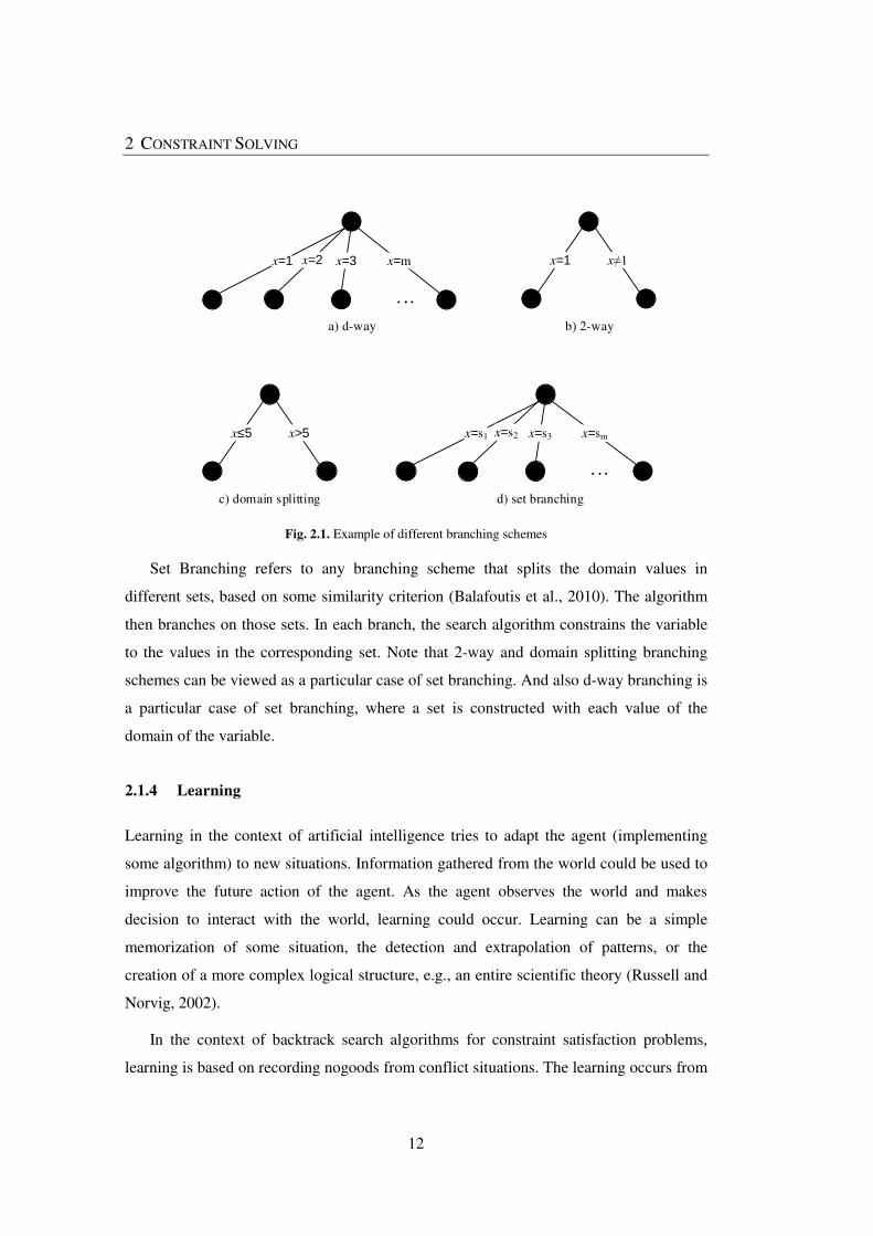
2.1.3 Branching schemes
At each node of the search tree, different branching schemes could be used. In Fig. 2.1
we can see graphically the four different branching schemes. Two traditional and widely
used branching schemes are the d-way and 2-way. In the first one, at each node, branches
are created, one branch for each of the possible values of the domain of the variable
associated with the node. Branches correspond to assignments of values to variables. In
the 2-way branching scheme two branches are created out of each node. In this scheme a
value vk is selected from the domain Dk of a variable xk, associated with the node. The left
branch corresponds to the assignment of the value to the variable, and the right branch is
the refutation of that value. This can be viewed as adding the constraint xk=vk to the
problem, in the left branch; or, if this fails, adding the constraint xk≠vk to the problem, in
the right branch. An important difference in these two schemes is that in d-way branching
the algorithm has to branch again on the same variables until the values of the domain are
exhausted. In 2-way branching, when a value assignment fails, the algorithm can choose
to branch on any other unassigned variable.
Another branching scheme is domain splitting (Dincbas et al., 1988). This scheme
splits the domain of the variable into two sets, typically based on the lexicographic order
of the values. Two branches are created out of each node, one for each set. A value vk is
selected from the domain Dk of a variable xk, associated with the node. Typically, in the
left branch the variable xk is constrained to the left part of the domain, which corresponds
to adding the constraint xk ≤ vk. In the right branch the variable xk is constrained to the
right part of the domain, which corresponds to adding the constraint xk > vk. Generally, in
each branch the other set of values is removed from the domain of the variable. Note that
the algorithm evolves by reducing the domains of the variables, and an assignment only
occurs when the domain size of a variable is reduced to one. Note also that this scheme
results in a much deeper search tree. This may be useful when the domains sizes of the
variables are very large.
2 CONSTRAINT SOLVING
12
x≤5 x>5
x=1 x≠1x=1 x=mx=2 x=3
. . .
x=s1 x=smx=s2 x=s3
. . .
a) d-way b) 2-way
c) domain splitting d) set branching
Fig. 2.1. Example of different branching schemes
Set Branching refers to any branching scheme that splits the domain values in
different sets, based on some similarity criterion (Balafoutis et al., 2010). The algorithm
then branches on those sets. In each branch, the search algorithm constrains the variable
to the values in the corresponding set. Note that 2-way and domain splitting branching
schemes can be viewed as a particular case of set branching. And also d-way branching is
a particular case of set branching, where a set is constructed with each value of the
domain of the variable.
2.1.4 Learning
Learning in the context of artificial intelligence tries to adapt the agent (implementing
some algorithm) to new situations. Information gathered from the world could be used to
improve the future action of the agent. As the agent observes the world and makes
decision to interact with the world, learning could occur. Learning can be a simple
memorization of some situation, the detection and extrapolation of patterns, or the
creation of a more complex logical structure, e.g., an entire scientific theory (Russell and
Norvig, 2002).
In the context of backtrack search algorithms for constraint satisfaction problems,
learning is based on recording nogoods from conflict situations. The learning occurs from
2.1 CONSTRAINT SATISFACTION PROBLEM
13
observation of the conflict situation and the nogood is created to explain the conflict.
These nogoods can be viewed as a safeguard of the conflict, ensuring that the conflict
does not occur again in the future.
Nogood recording was introduced in (Dechter, 1990), where a nogood is recorded
when a conflict occurs during a backtrack search algorithm. Those recorded nogoods
were used to avoid exploration of useless parts of the search tree.
Standard nogoods correspond to variable assignments, but more recently, a
generalization of standard nogoods, that also uses value refutations, has been proposed by
(Katsirelos and Bacchus, 2003, 2005). They show that this generalized nogood allows
learning more useful nogoods from global constraints. This is an important point since
state of the art CSP solvers rely on heavy propagators for global constraints. The use of
generalized nogoods significantly improves the runtime of CSP algorithms. It is also
important to notice that these generalized nogoods are very much like clause recording in
SAT solvers.
Recently, the use of standard nogoods and restarts in the context of CSP algorithms
was studied (Lecoutre et al., 2007a, 2007b). They record a set of nogoods after each
restart (at the end of each run). Those nogoods, named nld-nogoods, are computed from
the last branch of the search tree. So, the already visited tree is guaranteed not to be
visited again. This approach is similar to one already used for SAT, where clauses are
recorded, from the last branch of the search tree before the restart (search signature)
(Baptista et al., 2001). Recorded nogoods are considered as a unique global constraint
with an efficient propagator. This propagator uses the 2-literal watching technique
introduced for SAT (Moskewicz et al., 2001). Experimental results show the
effectiveness of this approach. More recently (Jimmy H. M. Lee et al., 2016) show that
nld-nogoods, in a reduction version, are increasing. And (Glorian et al., 2017) propose
different ways to reason with those increasing nogoods.
A hybrid approach, known as Lazy Clause Generation, that combines modelling and
search of CP(FD) with learning and restarts of SAT solvers is proposed in (Feydy and
Stuckey, 2009). The resulting solver is able to tackle problems that are beyond the scope
2 CONSTRAINT SOLVING
14
of CP(FD) and SAT. They conclude that the combination of CP(FD) search with learning
can be extremely powerful.
Learning general constraints, proposed in (Veksler and Strichman, 2015, 2016), is a
stronger form of learning which, instead of learning generalized nogoods, learns
constraints. This new learning scheme is inspired on conflict analysis of SAT solvers. It
traverses a conflict graph backwards for constructing a conflict constraint. Inference rules
for different types of constraints are used for the construction of the learned constraint.
Still, as the authors explain, this is an initial work and needs further developments of new
inference rules for other types of constraints. They present promising results of this
learning scheme, which is implemented for some constraints in the state of the art Haifa
CSP solver (Veksler and Strichman, n.d.). This CP(FD) Solver uses techniques from
SAT, namely, a variable selection heuristic similar to vsids (Moskewicz et al., 2001), a
phase saving mechanism (Pipatsrisawat and Darwiche, 2007), restarts and learning. It is
somehow related with our work, since it uses restarts, learning (a different scheme) and
heuristics based on learning.
2.1.5 Examples of CSP Problems
In this section we will present some CSP problems and show how they could be modeled.
The presented problems are the ones that we will use in our empirical study. So, besides
explaining the problems we also present and explain how the problems are modeled using
the Comet System.
The Comet system was the solver that we used in this thesis to implement and test our
proposed solutions. So, we will use this section for presenting and explaining how we
model the used problems in Comet. We will use the first problem to explain some
relevant parts of the Comet language.
2.1.5.1 N-Queens
The n-queens problem is the problem of putting n queens in an n by n matrix,
representing a chessboard, such that the queens do not attack each other. This is problem
number 54 from CSPLIB (Hussain, n.d.). In Fig. 2.2 we can see two examples of this

2.1 CONSTRAINT SATISFACTION PROBLEM
15
problem of size n, i.e., putting 4 queens in an n by n chessboard. The fist example, a)
solution, represents a solution for the problem, since all the queens are in a cell they do
not attack each other. In the second example, b) conflict, the two queens in the third and
fourth column are attaching each other in the diagonal, which configures a conflict
situation. Hence, this second example is not a solution for the problem.
♛
♛
♛
♛ ♛
♛
♛
♛
a) solution b) conflict Fig. 2.2. Example of n-queens problem
To model the n-queens problem we use one variable for each column. Hence, the
variables x1, …, xn, represent the columns of the chessboard. Each column can only have
one queen, so, each variable contains the number of the row where the queen is. Thus, the
domain of each variable is the possible rows, i.e., the set {1, …, n}.
For implementing the chess rule of non-attacking queens we must create constraints
specifying that, for each queen, there are no more queens in the same row, nor in the
same diagonal. For the first case we must guarantee that variables of the problem have
different values, i.e., have different rows. We could define a constraint, for each pair of
variables, specifying that each variable in the pair are different,
xi ≠ xj, where 1 ≤ i,j ≤ n and i < j
We must also ensure that two variables are not in the same diagonal. First, note that
the difference between the row of the queen and its variable number define a specific
downward diagonal, and the sum refers to a specific upward diagonal. So, using this
property, we could define two constraints, for each pair of variables, specifying that the
variables in the pair are not in the same diagonal. It is necessary to define one constraint
for each type of diagonal,
2 CONSTRAINT SOLVING
16
xi – i ≠ xj – j, where 1 ≤ i,j ≤ n and i < j
xi + i ≠ xj + j, where 1 ≤ i,j ≤ n and i < j
Of course, in practical terms, if the solver allows global constraints, it is better to use
them. For this problem, instead of using the binary constraints for all the pairs we use
only alldifferent global constraints. So, we end up with the following three constraints,
alldifferent(x1, x2, …, xn)
alldifferent(x1 – 1, x2 – 2, …, xn – n)
alldifferent(x1 + 1, x2 + 2, …, xn + n)
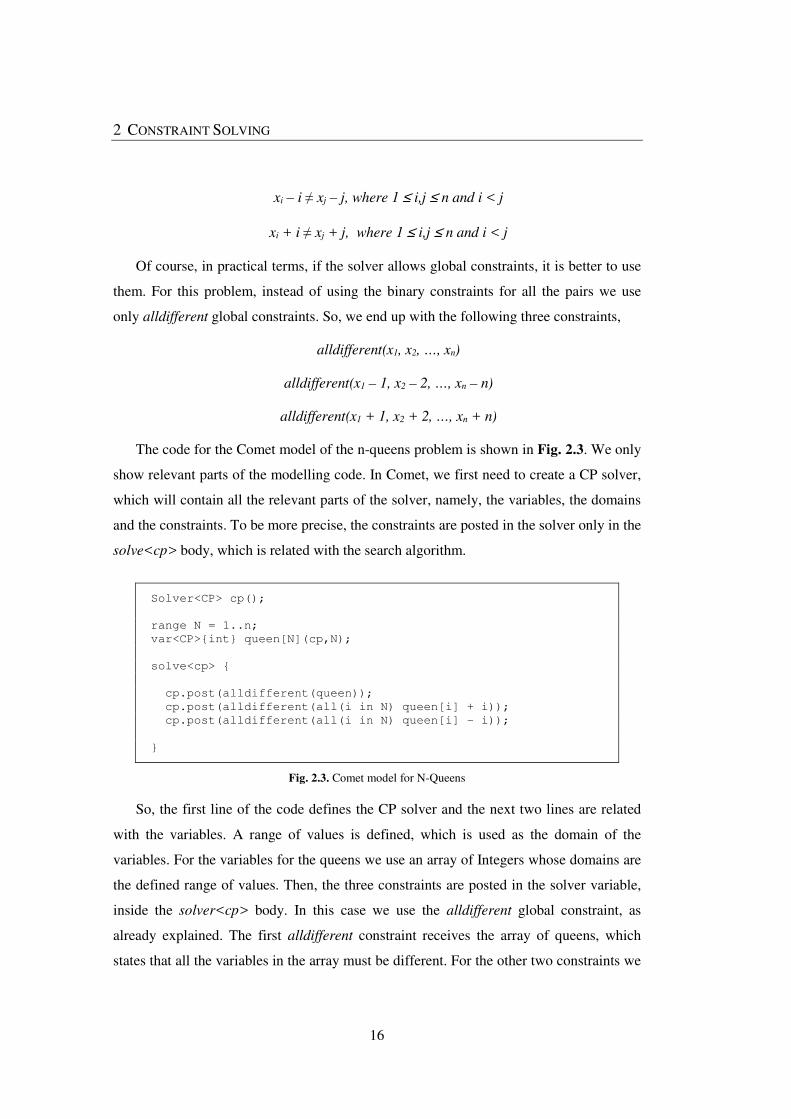
The code for the Comet model of the n-queens problem is shown in Fig. 2.3. We only
show relevant parts of the modelling code. In Comet, we first need to create a CP solver,
which will contain all the relevant parts of the solver, namely, the variables, the domains
and the constraints. To be more precise, the constraints are posted in the solver only in the
solve<cp> body, which is related with the search algorithm.
Solver<CP> cp();
range N = 1..n;
var<CP>{int} queen[N](cp,N);
solve<cp> {
cp.post(alldifferent(queen));
cp.post(alldifferent(all(i in N) queen[i] + i));
cp.post(alldifferent(all(i in N) queen[i] - i));
}
Fig. 2.3. Comet model for N-Queens
So, the first line of the code defines the CP solver and the next two lines are related
with the variables. A range of values is defined, which is used as the domain of the
variables. For the variables for the queens we use an array of Integers whose domains are
the defined range of values. Then, the three constraints are posted in the solver variable,
inside the solver<cp> body. In this case we use the alldifferent global constraint, as
already explained. The first alldifferent constraint receives the array of queens, which
states that all the variables in the array must be different. For the other two constraints we

2.1 CONSTRAINT SATISFACTION PROBLEM
17
do not have arrays, but Comet language allows the creation of arrays on the fly. This is
what is done in the last two posts, an array is created with variables having the difference,
in one case, and the sum, in the other case. Then, the alldifferent constraint guarantees, in
each case, that variables must be different.
2.1.5.2 Magic square and Talisman Square
A magic square of size n is an n by n matrix with all the numbers from 1 to n2, such that
the sum of each row, column and the two main diagonals are equal to a known magic
constant. This is problem number 19 from CSPLIB (Walsh, n.d.). The magic constant is
computed as
1
2 ���� + 1�
An example of a magic square can be seen in Fig. 2.4. Because it is a 4 by 4 square,
all the cells have different numbers from 1 to 16. The magic square, in this case, is 34 and
can be easily checked that it corresponds to the sum of the number in each column, rows
and the two main diagonals.
16 3 2 13
5
9
4
10 11 8
6 7 12
15 14 1
Fig. 2.4. Example of a Magic Square
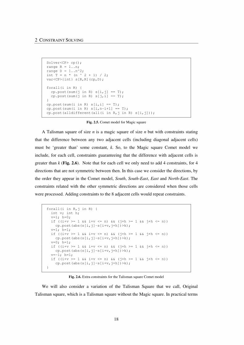
The Comet model for the Magic square is presented in Fig. 2.5 (note that, for
simplicity we eliminate the solve(cp) scope). To model the magic square we need n2
variables, one for every position of the matrix, hence we use a two-dimensional array for
the variables. The domain of those variables are all the possible numbers, i.e., the set {1,
…, n2}. We need to add constraints for the sums of all the n rows, n columns, and the two
diagonal main diagonal. Finally, an alldifferent constraint is used for all the variables, so
that we do not have positions (variables) with the same numbers.
2 CONSTRAINT SOLVING
18
Solver<CP> cp();
range R = 1..n;
range D = 1..n^2;
int T = n * (n ^ 2 + 1) / 2;
var<CP>{int} s[R,R](cp,D);
forall(i in R) {
cp.post(sum(j in R) s[i,j] == T);
cp.post(sum(j in R) s[j,i] == T);
}
cp.post(sum(i in R) s[i,i] == T);
cp.post(sum(i in R) s[i,n-i+1] == T);
cp.post(alldifferent(all(i in R,j in R) s[i,j]));
Fig. 2.5. Comet model for Magic square
A Talisman square of size n is a magic square of size n but with constraints stating
that the difference between any two adjacent cells (including diagonal adjacent cells)
must be ‘greater than’ some constant, k. So, to the Magic square Comet model we
include, for each cell, constraints guaranteeing that the difference with adjacent cells is
greater than k (Fig. 2.6). Note that for each cell we only need to add 4 constraints, for 4
directions that are not symmetric between then. In this case we consider the directions, by
the order they appear in the Comet model, South, South-East, East and North-East. The
constraints related with the other symmetric directions are considered when those cells
were processed. Adding constraints to the 8 adjacent cells would repeat constraints.
forall(i in R,j in R) {
int v; int h;
v=1; h=0;
if ((i+v >= 1 && i+v <= n) && (j+h >= 1 && j+h <= n))
cp.post(abs(s[i,j]-s[i+v,j+h])>k);
v=1; h=1;
if ((i+v >= 1 && i+v <= n) && (j+h >= 1 && j+h <= n))
cp.post(abs(s[i,j]-s[i+v,j+h])>k);
v=0; h=1;
if ((i+v >= 1 && i+v <= n) && (j+h >= 1 && j+h <= n))
cp.post(abs(s[i,j]-s[i+v,j+h])>k);
v=-1; h=1;
if ((i+v >= 1 && i+v <= n) && (j+h >= 1 && j+h <= n))
cp.post(abs(s[i,j]-s[i+v,j+h])>k);
}
Fig. 2.6. Extra constraints for the Talisman square Comet model
We will also consider a variation of the Talisman Square that we call, Original
Talisman square, which is a Talisman square without the Magic square. In practical terms

2.1 CONSTRAINT SATISFACTION PROBLEM
19
we remove from the Talisman square the constraints related with the sum of the magic
constant. Of course, the constraint guaranteeing that all the variables of the matrix are
different is maintained.
2.1.5.3 Latin squares
A Latin square of size n is an n by n matrix, such that each row and column has the
numbers 1 to n without repetition. This is described in problem number 3 of the CSPLIB
(Pesant, n.d.).
3 1 2 4
4
1
2
2 3 1
3 4 2
4 1 3
3
2
4
4 2
1
a) filled b) partially filled Fig. 2.7. Example of Latin squares
In Fig. 2.7 we can see two examples of Latin squares of size 4. The first one is fully
filled with the numbers 1 to 4 in each row and column, without repetition. The second
one is partial filled, maintaining, for the already filled numbers, the same constraints in
each row and column.
Solver<CP> cp();
range R = 1..n;
range D = 0..n-1;
var<CP>{int} s[R,R](cp,D);
forall(i in R) {
cp.post(alldifferent(all(j in R) s[i,j]));
cp.post(alldifferent(all(j in R) s[j,i]));
}
Fig. 2.8. Comet model for Latin square
The Comet model for this problem is presented in Fig. 2.8. It has n2 variables, one for
every position of the matrix, whose domain is the set {1, …, n}. For each column and row
an alldifferent global constraint is used, to guarantee that no repetitions exist.
2 CONSTRAINT SOLVING
20
We also use a variation of this problem, called Quasigroup With Holes (QWH),
which is a partial filled Latin square where some cells have a pre-defined number. This
problem is known to be more difficult than the Latin squares.
The well-known Sudoku problem is a Latin square with additional alldifferent
constraints for the interior squares. A widely used Sudoku puzzle is a Latin square of size
9 with pre-defined numbers, and with nine interior squares of 3 by 3 where the numbers 1
to n must also occur without repetition. The Sudoku problems can be generalized to other
sizes, provided that the size is a perfect square, which guarantee the existence of the
interior squares.
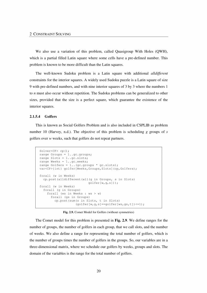
2.1.5.4 Golfers
This is known as Social Golfers Problem and is also included in CSPLIB as problem
number 10 (Harvey, n.d.). The objective of this problem is scheduling g groups of s
golfers over w weeks, such that golfers do not repeat partners.
Solver<CP> cp();
range Groups = 1..gc.groups;
range Slots = 1..gc.slots;
range Weeks = 1..gc.weeks;
range Golfers = 1..(gc.groups * gc.slots);
var<CP>{int} golfer[Weeks,Groups,Slots](cp,Golfers);
forall (w in Weeks)
cp.post(alldifferent(all(g in Groups, s in Slots)
golfer[w,g,s]));
forall (w in Weeks)
forall (g in Groups)
forall (ws in Weeks : ws > w)
forall (gs in Groups)
cp.post(sum(s in Slots, t in Slots)
(golfer[w,g,s]==golfer[ws,gs,t])<=1);
Fig. 2.9. Comet Model for Golfers (without symmetries)
The Comet model for this problem is presented in Fig. 2.9. We define ranges for the
number of groups, the number of golfers in each group, that we call slots, and the number
of weeks. We also define a range for representing the total number of golfers, which is
the number of groups times the number of golfers in the groups. So, our variables are in a
three-dimensional matrix, where we schedule our golfers by weeks, groups and slots. The
domain of the variables is the range for the total number of golfers.
2.1 CONSTRAINT SATISFACTION PROBLEM
21
The first set of constraints is used to ensure that all the golfers play in each week. It is
an alldifferent constraint for each week, stating that all the variables in that week is
different, so, golfers only play once in each week. The second set of constraints is used to
define that golfers do not repeat partners in different weeks.
This problem is known to have different symmetries. We do not present here
constraints for symmetry breaking, but we use constraints for breaking the most important
symmetries. Namely, we consider the following symmetries: players inside groups can be
exchanged; groups inside weeks can be exchanged; weeks can be exchanged; and players
can be renumbered.
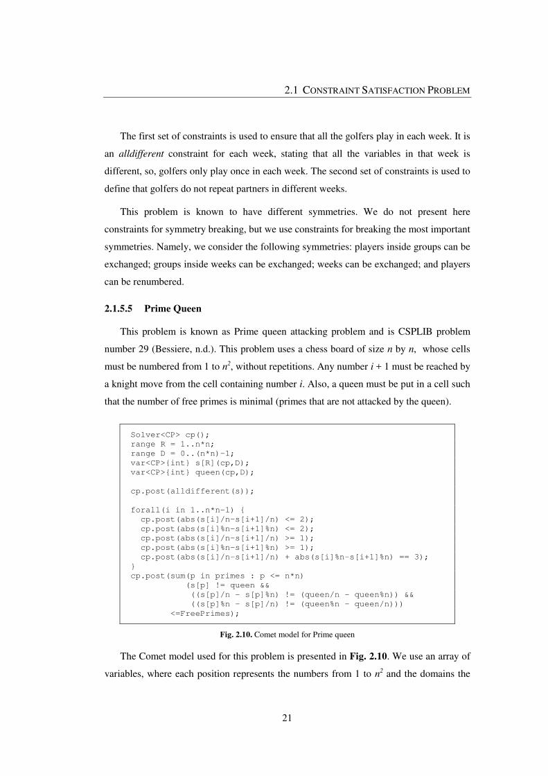
2.1.5.5 Prime Queen
This problem is known as Prime queen attacking problem and is CSPLIB problem
number 29 (Bessiere, n.d.). This problem uses a chess board of size n by n, whose cells
must be numbered from 1 to n2, without repetitions. Any number i + 1 must be reached by
a knight move from the cell containing number i. Also, a queen must be put in a cell such
that the number of free primes is minimal (primes that are not attacked by the queen).
Solver<CP> cp();
range R = 1..n*n;
range D = 0..(n*n)-1;
var<CP>{int} s[R](cp,D);
var<CP>{int} queen(cp,D);
cp.post(alldifferent(s));
forall(i in 1..n*n-1) {
cp.post(abs(s[i]/n-s[i+1]/n) <= 2);
cp.post(abs(s[i]%n-s[i+1]%n) <= 2);
cp.post(abs(s[i]/n-s[i+1]/n) >= 1);
cp.post(abs(s[i]%n-s[i+1]%n) >= 1);
cp.post(abs(s[i]/n-s[i+1]/n) + abs(s[i]%n-s[i+1]%n) == 3);
}
cp.post(sum(p in primes : p <= n*n)
(s[p] != queen &&
((s[p]/n - s[p]%n) != (queen/n - queen%n)) &&
((s[p]%n - s[p]/n) != (queen%n - queen/n)))
<=FreePrimes);
Fig. 2.10. Comet model for Prime queen
The Comet model used for this problem is presented in Fig. 2.10. We use an array of
variables, where each position represents the numbers from 1 to n2 and the domains the

2 CONSTRAINT SOLVING
22
position on the chessboard (the numbers from 0 to n2–1). We also need a variable for the
position of the queen. The first constraint is an alldifferent guaranteeing that all the
numbers are in different positions. Then, for each successive numbers (successive
position in the array of variables), we define a set of constraints which guarantee the
knight move.
This problem is formulated as an optimization problem, since it tries to minimize the
total number of free primes. Because our work is concerned with satisfaction problems
we transform this problem in a satisfaction problem. So, we add a constraint stating that
the number of free primes must be less than or equal than some constant. In this way it is
possible to solve various decision problems, each time with a smaller number of free
primes. The prime numbers are pre-computed and saved in the primes array.
2.1.5.6 Cattle Nutrition
This is a real world problem related with finding the best combination of Cattle food,
considering the nutritional requirements of Cattle. This problem is typically from the
Linear Programming area, but we have used a discrete representation of the continuous
variables of the problem, for use in the CP(FD) model.
Solver<CP> cp();
range D = 0..(maxGramas/gran)+1;
var<CP>{int} vars[R](cp,D); //one entry for each food
cp.post(sum(i in R)(vars[i]*(gran/1000.0)*infoAlimentos[i].ca)
<= necessidades.ca * (1+necessidades.eMax));
cp.post(sum(i in R)(vars[i]*(gran/1000.0)*infoAlimentos[i].ca)
>= necessidades.ca * (1-necessidades.eMin));
Fig. 2.11. Partial Comet model for Cattle Nutrition
For this problem, a set of different Cattle food is considered. Then, the purpose is to
define the amount of each type of food, such that a set of nutritional requirements
constraints are satisfied. We present in Fig. 2.11 a partial Comet model for this problem.
First, we define the discrete representation for the amount of food with a defined
granularity, gran. Then we use one array of variables with one position for each type of
food considered, and whose domain is the amount of food. We have a database of
2.2 SATISFIABILITY PROBLEMS
23
different Cattle food with nutrition information, which is used to select the nutrition
information of the used Cattle food and saved in the array infoAlimentos.
For each type of nutrition requirements we have two constraints, stating that the food
amount must be within a minimum and maximum value. In Fig. 2.11 we see an example
of such a constraint for the calcium requirements.
2.2 SATISFIABILITY PROBLEMS
2.2.1 Definition
A propositional satisfiability problem (SAT) is a particular case of a CSP where the
variables are Boolean, and the constraints are defined by propositional logic expressed in
conjunctive normal form. In spite of this relation, SAT is a well-known decision problem,
used for modeling combinatorial problems, and for which a full line of completely
independent research is in continuous growth. In any case, SAT and CSP share many
techniques and have benefited from each other developments (Bordeaux et al., 2006).
SAT was the first decision problem proved to be NP-Complete (Cook, 1971). It has
many applications to real world problems, since SAT algorithms have proved to be very
successful on handling large search spaces, due, primarily, to the ability of exploiting
problem structure (Marques-Silva, 2008).
Considering a propositional logic formula, the propositional satisfiability problem is a
decision problem trying to satisfy the formula using assignments to the variables of the
formula. More formally, consider the Boolean variables xi, i=1, …,n, of the propositional
logic formula; SAT can be defined by finding an assignment to all the Boolean variables
xi in the formula, such that the formula becomes a logical truth, i.e., satisfiable. Instead of
using propositional formulas expressed in the full syntax of propositional logic, SAT
uses, without loss of generality, formulas expressed in conjunctive normal form (CNF). A
CNF formula φ is a conjunction of clauses wi, i=1,…,m, where each clause is a
disjunction of literals. A literal is an occurrence of a Boolean variable xi or its negation
¬xi. To each Boolean variable xi, of the formula φ, the thruth value true (or 1 – one) or
2 CONSTRAINT SOLVING
24
false (or 0 – zero) can be assigned. A variable with no assigned value is said to be a free
variable. Accordingly, a literal can have a Boolean value or be a free literal. A clause (wi)
is said to be satisfied (wi=1) if at least one of its literals has the value true, unsatisfied
(wi=0) if all of its literals have the value false and unresolved otherwise (i.e., when it is
not possible to know the value of the clause). This last case occurs if none of the literals
have the value true, but some, and not all, have the value false. An unresolved clause with
only one free literal is said to be a unit clause. This type of clause plays an important role
in the search space reduction of the search algorithm, as it will be explained in the next
section. A CNF formula is said to be satisfied, φ = 1, if all its clauses are satisfied,
unsatisfied, φ = 0, if at least one of the clauses is unsatisfied. Otherwise, the formula is
unresolved, i.e., there are no unsatisfied clauses and at least one of the clauses is
unresolved.
To illustrate a SAT problem, let us consider the CNF formula, which has three
clauses,
φ=(x1 ˅ x2) ˄ (x1 ˅ ¬x3 ˅ ¬x2) ˄ (x3 ˅ ¬x2).
And the set of assignments
{ x1 = 0, x3 = 1}
Considering these assignments we rewrite the CNF formula φ with the Boolean
values instead of the variables
φ=(0 ˅ x2) ˄ (0 ˅ 0 ˅ ¬x2) ˄ (1 ˅ ¬x2).
So, those assignments make the first and second clause unresolved. In this case, these
two clauses are unit clauses, because all the literals, except one, have the value false. The
third clause is satisfied because one of the literals, x3, is true. Hence, the formula is
unresolved, because there are no unsatisfied clauses, some clauses (one in this case) are
satisfied and other clauses are unresolved, which per se does not allow us to know the
state of the formula.
For another example, consider again the same CNF formula φ and the set of
assignments
{ x1 = 1, x3 = 1}
2.2 SATISFIABILITY PROBLEMS
25
Considering now these assignments we rewrite the CNF formula φ with the Boolean
values instead of the variables
φ=(1 ˅ x2) ˄ (1 ˅ 0 ˅ ¬x2) ˄ (1 ˅ ¬x2).
In this case all the clauses are satisfied because all the clauses have one literal with
value true and, hence, the formula is satisfied.
2.2.2 Search Algorithms
As already referred the propositional satisfiability problem belongs to the well-known
NP-Complete class of problems. Algorithms for this class of problems have exponential
time complexity in the worst case, unless P = NP. The principal approach for solving
SAT is based on the Davis, Putnam, Logemann and Loveland (DPLL) procedure (Davis
et al., 1962; Davis and Putnam, 1960), which is basically a backtrack search algorithm
which implicitly searches a binary tree of decisions, defined by the 2n possible
assignments of the Boolean variables, where n is the number of variables in the problem.
In each node of the search tree a free Boolean variable is selected for branching. Out
of each node, two branches are created: one for the decision of assigning true; and the
other for the decision of assigning false to the selected variable. The selection of the
variable is typically based on heuristic selection, being vsids (variable state independent
decaying sum) the most widely used variable selection heuristic (Moskewicz et al., 2001)
and considered state-of-the-art. The order by which the two Boolean values are tested
may also depend on heuristics.
After each decision, some of the clauses could become unit clauses, which allows a
technique known as unit propagation (Davis and Putnam, 1960) to be applied. This
technique identifies necessary assignment for variables. A unit clause has only one free
literal (and all the others are false), so, to become satisfied it is necessary that the free
literal becomes true. Note that after implying the necessary Boolean value to a literal, and
as a consequence to the corresponding variable, other clauses can become unit clauses,
and so, unit propagation must also be applied to those unit clauses. Hence, unit
propagation must be applied iterctively, until all the unit clauses are exhausted (become
satisfied); this procedure is known as Boolean Constraint Propagation (BCP). Intuitively,
2 CONSTRAINT SOLVING
26
BCP reduces the search space, pruning branches of the search tree corresponding to the
implied variables.
The search tree maintains a partial solution to the problem, consisting of assignments
of Boolean values to the variables. When a node is reached where all the clauses become
satisfied, the search ends with a solution. But, if during the search a node is reached
where, at least, one unsatisfied clause exists, the search can no longer continue and the
search must backtrack to try other value combinations. The search backtracks to the most
recent node where only one of the two Boolean values has been tried. This form of
backtracking is known as chronological backtracking. If the search space is exhausted
without reaching the situation where all the clauses are satisfied, the problem has no
solution because the formula is unsatisfiable.
Other more interesting form of backtracking is non-chronological backtracking.
Instead of backtracking for the most recent node, it is able to backtrack to a node
identified as one of the causes of the conflict. This form of backtracking is used in state-
of-the-art SAT solvers and has the advantage of skipping irrelevant decisions for the
failure, which, in practice, corresponds to pruning irrelevant search tree branches. An
important form of non-chronological backtracking is known as Conflict-Directed
Backjumping and was introduced by (Prosser, 1993). Nevertheless, current SAT solvers
use a form of non-chronological backtracking that is associated with another very
important technique known as clause learning from conflicts.
Current solvers for SAT use an approach known as Conflict-Driven with Clause
Learning (CDCL), which extend the original DPLL procedure. This approach was first
introduced in the GRASP solver (Silva and Sakallah, 1996). It has conflict analyses, from
which the algorithm records clauses explaining the conflict; this is a form of learning and
is known as clause learning or clause recording. This learning gives the algorithm the
ability not to make the same mistakes again in the future. Also, instead of the simple
chronological backtracking to the preceding level of the search tree, conflict analyses
allow the algorithm to perform a non-chronological backtracking to the level where the
origin of the conflict is.
2.2 SATISFIABILITY PROBLEMS
27
When a conflict occurs, the CDCL algorithm identifies its causes. For this, the
algorithm maintains an implication graph created with the implied assignments, which
were made by the Boolean Constraint Propagation mechanism. The CDCL algorithm
identifies the conditions, by means of the set of assignments, which originate the conflict.
A new clause, that explains the conflict, is then created and recorded. This recorded
clause is known as conflict clause, or nogood, and is used by the CDCL algorithm in the
remainder of the search tree as part of the CNF formula. This conflict clause is a
safeguard, guaranteeing that the assignments that drive the search to a conflict do not to
happen again, hence, pruning the subsequent search tree.
Conflict clauses are recorded every time a conflict occurs. This could lead the
algorithm to run out of memory. Note that, in the worst case, the number of conflicts is
exponential in the number of variables, so, recording all the conflict clauses could be
impossible in practice. On the other hand, large conflict clauses are known to be of little
importance for pruning the search tree (Silva and Sakallah, 1996). So, in practice, SAT
solvers define conditions for deleting those larger conflict clauses.
The use of restarts is an important improvement on CDCL solvers (Baptista and
Silva, 2000), and is, currently, widely used. It continuously runs the search algorithm,
from the beginning, giving, on each run, a new opportunity for solving the problem.
Typically, the restart occurs when a cutoff value is reached; the search stops and then
starts again a new run. To guarantee algorithm completeness, the cutoff value is
incremented after each restart. Note that, because of clause recording of CDCL solvers,
after each restart the search no longer starts from scratch, it starts with learned clauses
retained from past runs.
Other very important improvements of CDCL solvers are the use of efficient data
structures and conflict driven selection heuristic (Moskewicz et al., 2001). The former
improvement uses an efficient data structure for detecting unit clauses in the BCP part of
the search algorithms, and is known as watched-literals. For each unresolved clause it
watches any two free literals (e.g., the first two). If one of those literals becomes false it
tries to watch other free literals. But if no more free literals exist, then the clause must be
unit, and the literal that must become true is the one that is still being watched. The main
advantage of this strategy is that it is not necessary to change the watched literals when
2 CONSTRAINT SOLVING
28
the search backtracks. The latter improvement uses the occurrence of variables in conflict
clauses, and also, from time to time, the occurrences of variables are divided by a
constant. This is a very low overhead variable selection heuristic that prefers variables
participating in recent conflicts and is known as variable state independent decaying sum
(vsids).
Due to non-chronological backtracking and restarts, trashing of good decisions can
occur, requiring the search to redo that same search space in the future. To avoid this loss
of decisions, a mechanism of decision caching can be used that makes the same decision
when the variable is selected. This was introduced in (Pipatsrisawat and Darwiche, 2007),
and is known as phase-saving, which is typically associated with rapid restarts.
2.3 SUMMARY AND FINAL REMARKS
Constraint Satisfaction Problems and Satisfiability Problems represent very important
areas of research within the broader area of Artificial Intelligence. They both are decision
problems and share many techniques. Still, they have independent research directions
which have resulted in different approaches in each area. In the context of our research
interest we highlight the widely use of restarts and learning in SAT algorithms compared
with the only emerging use in CP(FD) algorithms.
Learning, in the context of SAT algorithms is known as conflict clause recording and,
in the context of CP(FD) algorithms, it is known as nogood recording. It is an important
and wide use feature of SAT solvers algorithms. But for CP(FD), although being
important, it is not widely used. Important progress in SAT solvers was due to the use of
restarts associated with conflict clause recording (Baptista and Silva, 2000; Moskewicz et
al., 2001) and the use of heuristics based on conflict clauses along with reengineering of
SAT solvers with efficient data structures (Moskewicz et al., 2001).
29
3 HEURISTICS
As already discussed, backtrack search algorithms are widely used for solving constraint
satisfaction problems. A key element of these algorithms is the order in which variables
are selected for branching. Also, but not so important, is the order in which the values for
the selected variable are tested. As it is widely known, a bad decision on the next variable
to select could drive the search for unpromising regions of the search space. This results
in combinatorial explosions of the search space.
Near the root of the search tree, a bad decision has more impact, because a bigger tree
exists under that bad decision, and, consequently, a bigger search space explosion exists.
This is why good heuristic decisions are important near the root of the search tree.
Unfortunately, that is not always the case since, typically, at the beginning of search, the
heuristic is not well informed.
An adaptive heuristic can gather information from the already explored search space.
With that information we can tune the heuristic to become more informed. We still have
the problem of bad first decisions, occurring near the root of the search tree. But as the
search evolves, the problem of bad decisions near the root tends to fade away, due to
more informed decisions.
Having more informed decisions near the root is also a key factor for restarts. Rather
than starting again from scratch, when a restart occurs, the search starts again but now
3 HEURISTICS
30
making more informed decisions. We can see the impact of this when results are
discussed.
It is also important to notice that, in this thesis, we are not interested in problem
dependent heuristics. Our focus is on general purpose heuristics, that are independent of
the domain of the problem considered.
The remainder of this chapter is organized as follows. We start by comparing static
versus dynamic variable ordering heuristics. Then we focus on the important fail first
principle. Next we focus on weighted based heuristics and then we explain more recent
heuristic strategies. Finally we overview the more important SAT heuristics, namely the
one based on conflicts, as this is central in this thesis.
3.1 STATIC VERSUS DYNAMIC VARIABLE ORDERING HEURISTICS
Static variable ordering (SVO) heuristics only use information from the structure of the
initial problem, without using information from the ongoing search. The order for
selecting the branching variables is defined before the search and is fixed during the
search (this is why they are also called fixed variable ordering). This means that, at each
node of the search tree, the algorithm selects for branching the next free variable based on
the predefined ordering of the variables.
On the other hand, dynamic variable ordering (DVO) heuristics are branching
variable selection heuristic strategies that use information of the ongoing search to change
the ordering of the variables. Hence, at each node of the search tree, the algorithm selects
for branching the next free variable based on the current CSP at that point, which is
dependent on the (partial) assignment already made. This means that at each node a
different ordering can exist.
The most basic SVO heuristic selects the next branching variable based on the
lexicographical order (lex). So, by simply changing the names of the variables in the
problem model the search tree varies. As it is easily noticed this heuristic lacks structural
information of the problem and so it is not used by itself. Nevertheless this heuristic is
widely used in conjunction with other, more informed, heuristics, for breaking ties. It is a

3.2 THE FAIL FIRST PRINCIPLE
31
common situation, when different variables have the same heuristic value. Faced with
that situation, the backtrack search algorithm must break ties and chose only one of them.
Another widely used heuristic for breaking ties is the random ordering (rand), applied at
each branching node. This heuristic selects randomly among the variables with the best
value. As will be explained later, this heuristic is central for restarts. Also notice that the
rand heuristic can also be used by itself. In this case, and due to the void of information
within this heuristic, the backtrack search algorithm will perform a random search.
Another SVO heuristic, width, selects the next branching variable based on the
minimum width of the constraint graph (Freuder, 1982). Also using information from the
constraint graph in (Dechter and Meiri, 1989) Dechter and Meiri define a heuristic that
selects the next branching variable based on the maximum initial degree of the variables,
deg. This heuristic favors variables that are constrained with more of the other variables.
SVO heuristics suffer from an important weakness: they only use information from
the initial problem and that may not be enough to solve the problem. DVO heuristics try
to solve this question, since information is collected during the ongoing search, and so,
the heuristic is modified as the search evolves.
3.2 THE FAIL FIRST PRINCIPLE
Tring where it is most likely to fail and pruning the search space as soon as possible are
two important strategies that help tree searching for CSP (Haralick and Elliott, 1980). It
was also shown empirically that changing dynamically the variable search order, based on
the actual size of variable domains, has performance improvements, particularly when
forward checking is employed.
The fail first (FF) principle, applied to the variable selection heuristic, states that the
variable that is most likely to drive the search algorithm to a failure must be selected for
branching. The DVO heuristic based on the FF principle states that the next unbound
variable to select for branching is the one with the fewest possible values in the domain
(the minimum size of the domain), we call this heuristic dom. So, in this context,
employing the FF principle means that, dynamically, during the search, an optimal order

3 HEURISTICS
32
is choosen for the branching variables. This optimal order is done on a local basis
(domain sizes) and will lower the number of expected consistency tests, when compared
with a random order (Haralick and Elliott, 1980).
The topology of the search tree is defined by the order in which branching variables
are selected. In (Haralick and Elliott, 1980), from experimental results, it was shown that,
changing the search order of the selected branching variables, the search efficiency can be
influenced. This search efficiency was measured by branch depth. They showed that,
choosing the next branching variable having the smallest remaining domain (dom) always
minimizes the expected branch depth, leading to a more efficient search (tree).
The DVO heuristic dom is an implementation of the FF principle, that chooses for
branching the next unbound variable that has the smallest remaining domain size. As the
backtrack search algorithm evolves, the size of the yet unbound variables changes.
Selecting variables trigger the constraint propagation mechanism and, as a consequence,
values can be wiped out from the domains of the remaining unbound variables, due to
being inconsistent with the current partial assignment. On the other hand, when the
algorithm backtracks, the values are recovered.
In spite of the dom heuristic being dynamic, it is still biased by initial decisions. If the
heuristic values in the beginning of the search are not sufficiently discriminated, the
search can be compromised, since the poor initial decisions can drive the search to
unsolvable parts of the search space. We can say, in these cases that the fail first principle
was indeed not applied, compromising the future search. Of course, if the search is on a
correct path, the algorithm should stay on it. But, if it is on an incorrect path, then the
algorithm, due to the FF principle, should fail as soon as possible. Even in this case, if the
algorithm is deep in the search thee, it may still be insufficient, due to of the already
ongoing combinatorial explosion of the search tree.
Other heuristics exist based on the FF principle, that are variations of the dom
heuristic. In (Frost and Dechter, 1994) they first use the deg heuristic when the initial
domain size of the variables is the same. After that, they use the standard dom heuristic.
This heuristic, which we call dom+deg, could minimize the already discussed problem of
3.2 THE FAIL FIRST PRINCIPLE
33
uninformed initial branching decisions, since the first decision is more informed, when
the dom heuristic comprises no information.
The search can be improved when combining the domain size and information from
the constraint graph structure. In (Bessière and Régin, 1996) they present a branching
variable heuristic, dom/deg, that combines information from variable domain sizes and
variable degree. This heuristic chooses the minimum value of the ratios dom/deg. It was
shown that this new heuristic is more efficient than the dom+deg.
A heuristic similar with dom had been proposed before dom, but now in the context
of a new method for graph coloring (Brélaz, 1979). It is known as brelaz, because of the
name of the author. This heuristic selects the next branching variable based on dom, and
breaks ties maximizing the dynamic degree (ddeg) of the variable. The dynamic degree of
the variable is also known as the future degree or actual degree. The ddeg heuristic selects
the variable that constrains the largest number of unbound variables.
In (Smith and Grant, 1998) they further study the FF principle, particularly the
dom/deg and dom/ddeg heuristic. It was argued that the success of dom and related
heuristics is not only due to the FF principle, and must also be explained by other reasons.
In (Haralick and Elliott, 1980) it was shown that the expected branch depth is minimized
when the branching heuristic chooses the variable with the smallest probability of
succeeding, which is the one with the smallest domain size. Assuming that the FF
principle is an important strategy, then a more informed FF strategy must have better
results. So in (Smith and Grant, 1998) they study variations of the dom heuristic, based
on the idea that variables that constrain many future variables (i.e. using the variable
degree) are more likely to drive the search to a failure. They create heuristics with more
informed FF strategies, which have a greater probability to reduce the search depth.
Unfortunately they could not conclude that the search depth is reduced when using more
informed FF strategies. Nevertheless, in (Beck et al., 2004, 2005) a deeper analysis of
(Smith and Grant, 1998) was made that confirms that the proposed heuristics indeed
increase the ability to fail first, which means, reduce the search depth. But, unfortunately
this does not imply a better search effort; thus, other reasons must exist that influence the
search efficiency.
3 HEURISTICS
34
The dom heuristic is central in the implementation of the fail first principle. And the
FF principle is still up to date and widely used. Even if there are other principles that
must be considered in the implementation of better variable selection heuristics, it will
not refute the FF principle. As already discussed, one of the main problems of dom is in
the beginning of the search tree, when the domains of variables happen to be of the same
size. This problem can be overcome by associating another variable selection heuristic,
which could be more informed in the beginning of the search tree. As we will see, this is
what we do in the heuristics proposed in this thesis. It is easy to see that one of the main
advantages of the dom heuristic is its computational efficiency. We only need to count the
number of values in the domain of the variables, and these counters are easily updated
during search.
3.3 WEIGHTED BASED (CONFLICT-DRIVEN) HEURISTIC
A generic heuristic based on weighting constraints involved in conflicts was proposed in
(Boussemart et al., 2004). This is a DVO heuristic which has the ability of guiding the
backtrack search algorithm toward hard parts of the search space. Traditional DVO
heuristics use only local information, from the current state of the search. But the
proposed heuristic can use information from the already searched space. This heuristic
uses information related to the number of times the constraint fails. It selects for
branching the variable involved in more failed constraints, and is called wdeg. They show
that the number of times each constraint is violated is an important indicator of
inconsistent parts of the search space.
The wdeg heuristic associates a weight to each constraint as a way of identifying
constraints that frequently participate in fails. During the search, whenever a constraint
fails, its weight is incremented. The main goal of this heuristic is to identify constraints
that are more important than others, because they are harder to satisfy. This heuristic is
able to drive the search to hard (inconsistent) parts of the search space.
The novel approach in this heuristic, as argued in (Boussemart et al., 2004), is that it
learns from past fails (a look-back technique) and then uses that learning to guide the
backtrack search algorithm (a look-ahead technique). As the search evolves, the weights
3.3 WEIGHTED BASED (CONFLICT-DRIVEN) HEURISTIC
35
of hard constraints will grow more than the other constraints, because they are
participating in more conflicts. Using that information, the wdeg heuristic will drive the
search to the hard parts of the search, by selecting variables involved in more higher
weighted constraints. It is easy to see that the heuristic will be more accurate as the search
evolves.
To implement this heuristic we need to have a counter for each constraint, the weight
of the constraint, initialized to 1. During search, each time the domain of a variable
becomes empty (a failure) the counter of the constraint, responsible for the domain wipe-
out, is incremented by 1. The wdeg heuristic uses these counters to compute the weighted
degree for each variable. For each variable, its weighted degree is the sum of the weights
of the constraints in which it participates. The wdeg heuristic selects for branching the
variable with the greatest value. It is important to observe that this heuristic is an
implementation of the FF principle, since it tries to first examine inconsistent parts of the
search space, i.e., tries to fail as soon as possible.
In (Boussemart et al., 2004) a heuristic was also proposed that combines the current
domain sizes (dom) with the current weighted degrees (wdeg). This heuristic selects for
branching the variable with the smallest ratio dom/wdeg. The branching variable
heuristics wdeg and dom/wdeg are called conflict-directed, because they use information
from conflicts. It was shown that these conflict-directed heuristics are the most efficient
ones (Boussemart et al., 2004).
One final note to discuss two potential weaknesses of the wdeg based heuristics: one
related with the order of constraint propagation; and the other related with the use of
global constraints. Related to the first case, a failure occurs as a result of a series of
propagations whose order is dependent on the implementation. So, as a result, the
constraint identified as responsible by the failure is dependent on the specific order.
Because of this, the wdeg heuristic is sensitive to the specific order of the propagation.
The wdeg based heuristics were proposed in the context of binary constraints, and the
natural approach for dealing with global constraints is to increment the weight of every
variable in the failed constraint. That is, treat the global constraints in the same way. This
means that the conflict information will be dispersed, because it will disturb the weights
3 HEURISTICS
36
of variables that are not involved in the conflict. As an extreme example, consider a
hypothetical problem that can be modeled by a single alldifferent constraint or,
alternatively, by various different binary constraints. In the first model, the wdeg heuristic
is useless, since we only have one constraint involving all the variables, and each time the
constraint fails, all the variables will reflect equally the increment of the constraint
weights. On the other hand, in the second model, the wdeg heuristic has the possibility of
having different constraint weights and, as a consequence, having different variables
weights, for making a more informed heuristic decision. We can say that wdeg based
heuristics are biased by the specific problem model, in particular if the model makes
intensive use of global constraints.
3.4 OTHER STATE OF THE ART HEURISTICS
A general purpose search strategy that uses the notion of impact of a variable was
proposed in (Refalo, 2004). It is based on techniques from integer programming. The
impact of a variable is related with the ability of the variable for reducing the search
space. During the ongoing search, reductions of the domains of variables, due to variable
assignments, are used for defining the impact of the variable. This strategy is used with
restarts, which is crucial for performance improvements. This is because, each time the
search restarts, the impact of variables (heuristic) is more accurate, which is particularly
important near the root of the search tree.
To be more precise, the impact is a value that measures the reduction of search space
for one particular assignment (of a domain value to the variable). And the impact of a
variable is a combination of the impacts of all possible assignments for that variable. See
(Refalo, 2004) for details on the formulation. The impact heuristic selects for branching
the variable that maximizes the impact and the value to assign the one that minimizes the
impact of all assignments. It was shown that this heuristic outperforms the dom heuristic
(restarts are not used with this heuristic) in the tested problems.
Another idea for variable branching heuristics is using the activity of variables in the
constraint propagation part of the search algorithm (Michel and Hentenryck, 2012). This
activity-based search (abs) favors variables that had their domains more times reduced,
3.4 OTHER STATE OF THE ART HEURISTICS
37
due to the propagation algorithm, after an assignment. Each variable has a counter (the
activity) for how many times its domain was reduced. At each node of the search tree,
counters are incremented for the variables that had its domain reduced. Also, there exists
an age decay parameter applied to every unbound variable, which allow to progressively
forget older values. The abs heuristic selects for branching the variable with the greatest
ratio of activity by domain size. Optionally, a value heuristic, that selects a value with the
smaller activity, could be applied. Additionally, restarts can be used, benefiting the search
after the restart, since the heuristic has more information (which is especially important at
the beginning of the search tree). They compared the abs heuristic with impact and wdeg,
concluding that abs is more robust and sometimes has performance improvements.
The concept of counting-based search heuristics was introduced in (Zanarini and
Pesant, 2009). In (Pesant et al., 2012) different generic heuristics were studied based on
that concept. One of them, maxSD, was shown to outperform, in many cases, dom,
dom/wdeg and impact. These counting-based heuristics do not use local information, they
use global information related with constraints, counting the number of solutions. The
selection of branching variables tries to maintain most of the solutions (the maximum
number of solutions). This was done based on information from constraints, indicating
what proportion of the solution is maintained, considering the branching decision.
One final remark for a recent work related with conflict ordering search (cos) (Gay et
al., 2015), that is applied to scheduling problems, although the authors argue it is a
generic strategy. They propose a heuristic based on remembering the last branching
variables that led to a failure. Their work is very similar to ours, since it uses nogoods
recording from restarts in a domain splitting search. We will refer to this subject later on
this thesis.
In the cos heuristic, each variable has a stamp indicating the last time the variable was
involved in a conflict. In practical terms, when a conflict occurs, the number of conflicts
(counter for the number of conflicts that already happened) is recorded in the stamp of the
last decision variable. In the beginning of the search an initial ordering of the variables is
used, based on some specific heuristic. The cos heuristic selects for the next branching
variable the one with the higher stamp. But if none of the unbound variables have a
stamp, then the specific heuristic is used. Hence, as the search evolves and conflicts start
3 HEURISTICS
38
to occur, the specific heuristic is replaced by the order of conflicts (the stamps). It was
shown that the generic cos heuristic is competitive in scheduling problems. Restarts are
also used, with the advantage of starting the search from scratch again (after a restart), but
now with a more informed heuristic. Unfortunately, as reported, the use of restarts does
not seem to make a difference.
3.5 SAT HEURISTICS
The work presented in this thesis is inspired in the successful use of restarts in backtrack
search algorithm for SAT. One of the important components of that success is the
branching heuristic. So, it is important to present an overview of SAT branching
heuristics, with special focus on vsids (Moskewicz et al., 2001), which was introduced
about sixteen year ago, but it is still considered state of the art.
In SAT, the most basic branching heuristic selects randomly among the unassigned
variables and also selects randomly the value to assign. But the most important heuristics
use dynamic information collected during the ongoing search. In (Silva, 1999), a
comprehensive study of state of the art branching heuristics, at that date, was made.
Based on this paper we will briefly present some of the well-known SAT heuristics.
The mom branching heuristic was one of the most known and used branching
heuristics. It is based on the notion of maximum occurrences on clauses of minimum size.
The size of a clause is its number of literals. This heuristic prefers variables occurring, as
positive and negative literal, in a large number of the smallest non-satisfied clauses. This
relation is determined by a function that can have different arrangements. Also, another
variation is related to using the largest clauses instead of using the smallest clauses.
Intuitively, the reason for using the smallest clauses is because assigning values to
variables occurring in the smallest clauses is expected to induce other implied
assignments and, as a consequence, reduce the search space.
Other important branching heuristics are based on counting literals in unresolved
clauses. This is done dynamically at each step of the backtrack search algorithm, and, for
each variable, two counters exist. One counts the number of unresolved clauses in which
3.5 SAT HEURISTICS
39
the variable appears as a positive literal, Cp. The other counter is the same, but for
negative literals, Cn. The combination of these counters produces different heuristics. The
dynamic largest combined sum (dlcs) heuristic selects for branching the variable with the
largest sum Cp + Cn, and assigns to it the value true, if Cp ≥ Cn, or false otherwise. The
counters can be used separately and the heuristic selects for branching the variable with
the largest individual value. This heuristic is named dynamic largest individual sum
(dlis). The assignment of values is the same as dlcs. As argued in (Silva, 1999), for some
instances, the heuristics can make bad decisions, because it is too greedy. A random dlis
(rdlis), that selects the value to assign randomly, is a good compromise to prevent making
those bad decisions. From the study conducted in (Silva, 1999) the dlis heuristic seems to
be better because it presents more solid results, but, for some instances, even rand has
good results.
3.5.1 The vsids heuristic
In (Moskewicz et al., 2001) a new solver was presented, chaff, with improvements of
various components of search algorithms. It also includes a new lightweight branching
heuristic based on information from conflict clauses, recorded when a conflict exists and
that explains the reasons of the conflict (nogoods). This conflict-based branching decision
heuristic is named variable state independent decaying sum (vsids).
The vsids heuristic associates to each variable two counters, one for each positive and
negative literal polarity, which are initialized to zero. These counters will register, during
the ongoing search, the occurrence of the literals in conflict clauses. So, when a conflict
clause is added to the solver, as a result of a conflict, the counter associated to each of the
literals polarity in the clause is incremented. The vsids heuristic then chooses, for
branching, the unassigned variable and polarity (value to assign) with the highest counter.
By default, ties are broken randomly.
One important feature of this heuristic is the decaying sum. All the counters are
divided by a constant value, from time to time. Because the vsids strategy focuses on
variables involved in conflicts, it can be viewed as trying to satisfy conflict clauses. But,
because the counters are all divided, the more recent conflict clauses have more
3 HEURISTICS
40
significance in the counters. So, more accurately, this heuristic can be viewed as trying to
satisfy the recent conflict clauses.
As explained in (Moskewicz et al., 2001) one of the key properties of the vsids
heuristic exploits the fact that conflict clauses are indeed what primarily drives the search
on difficult problems. Another key property is the very low computational overhead.
Indeed, using this heuristic dramatically improves the performance of the algorithm on
the hardest problems, at least by one order of magnitude. All this is achieved without
deteriorating performance on the easier problems.
The vsids heuristic does not work by itself; it works in conjunction with other
strategies – Obviously, nogoods in the form of conflict clause recording, and a frequent
restart strategy. When a restart occurs, the search algorithm starts again, but now with
new information obtained from the previous conducted search, in the form of clause
recording and variable counters. The restart offers a way of changing early bad decisions.
The vsids strategy is still state of the art in backtrack search algorithms for solving
SAT (Biere and Fröhlich, 2015). Because of the success of this strategy we tried to use it
in our work. In fact, to some extent we managed to include the vsids strategy in backtrack
search algorithms for CSP, using information from nogoods.
3.6 SUMMARY AND FINAL REMARKS
A very important decision heuristic in SAT is based on conflict clause recording
(Moskewicz et al., 2001). This heuristic is named vsids, and the general idea is to
increment the value of the literals involved in conflicts. The heuristic then selects the
variable involved in more conflicts. In (Moskewicz et al., 2001) the use of this heuristic,
restarts, nogoods and efficient data structures, boosts the SAT solver performance. This
heuristic can be viewed as a conflict driven heuristic, since it is based on existence of
conflicts. We can also interpret this heuristic as a fail-first type, because it tries to reward
variables that are involved in conflicts, hence, drives the search to where is more probable
that it will fail.

3.6 SUMMARY AND FINAL REMARKS
41
The wdeg heuristic is also a conflict driven heuristic for CP(FD). But this heuristic is
very different from vsids, since it rewards variables directly involved in conflict, i.e.,
variables occurring in the constraint that has failed. Note the fundamental difference with
vsids, which rewards variables that occur in conflict clauses (nogoods).
In CP(FD), state of the art heuristics do not use information from nogoods. So, using
this information could be a key factor for progresses on using restarts in CP(FD). And
due to the very good results in SAT, the use of conflict-driven heuristics, restarts and
nogoods should be investigated in CP(FD) solvers.

43
4 RESTARTS
Restarts, used in the context of non-deterministic algorithms, means that one run of the
algorithm is stopped and then the algorithm is started again from the beginning. The
algorithm is stopped typically because it is lost, so, starting again offers a new
opportunity for the algorithm to find a solution. Obviously, the algorithm must be a non-
deterministic one, otherwise the new run will repeat the same unsuccessful execution.
The use of restarts is a key aspect for solving Propositional Satisfiability Problems
(SAT). It has boosted SAT search algorithms (Baptista and Silva, 2000; Moskewicz et al.,
2001), and is now widely used and considered essential for solving SAT. But in
constraint programming over finite domains (CP(FD)), although it is starting to be used,
it is not widely used nor it is a key technique for solving CP(FD). This is a main
motivation for this thesis, since we believe that restarts should be of relevant importance
for CP(FD) algorithms as they are for SAT algorithms. Probably it would not be in the
same way nor with all the same interplay of techniques. But some of the techniques of
SAT could also be used with success in CP(FD).
The first time the restarts technique was used to solve SAT was in (Selman et al.,
1992). Here, a greedy local search algorithm, named GSAT, is used. The algorithm
restarts after reaching a fixed number of iterations without finding a solution. This is a

4 RESTARTS
44
non-deterministic algorithm because it uses randomization in different parts of the search,
e.g., for starting from different states and for breaking ties. And also, because of the very
nature of local search, it is an incomplete algorithm.
In this thesis we are interested in backtrack search algorithms. Randomization is a key
aspect for implementing restarts because it introduces the necessary non-deterministic
behavior. A backtrack search algorithm is randomized by introducing a fixed amount of
randomness in the branching heuristic (Gomes et al., 1998). The utilization of
randomization results in different sub-trees being searched each time the search algorithm
is restarted.
For many combinatorial problems, different executions of a randomized backtrack
search algorithm on the same instance can result in extremely different runtimes. This
large variability in the runtime of search procedures can be explained by the phenomenon
of heavy-tail distribution (Gomes et al., 1997, 1998, 2000). A randomized search
algorithm can be repeatedly run (restarted), each time limiting the maximum number of
backtracks to a cutoff value. In practice, this strategy and a good cutoff value eliminates
the heavy-tail phenomenon, but unfortunately such a value has to be found empirically
(Gomes et al., 1998). If restarts are used with a fixed cutoff value, the resulting algorithm
is not complete. A solution to this problem is to implement a policy for systematically
increasing the cutoff value (Walsh, 1999). A simple policy is to increment by a constant
the cutoff value after each restart. The resulting algorithm is complete, and thus able to
prove unsatisfiability (Baptista and Silva, 2000).
However, the incremental cutoff policy still exhibits a key drawback, because paths in
the search tree can be visited more than once. This was addressed for SAT problems in
(Baptista et al., 2001) and for CSP in (Lecoutre et al., 2007a, 2007b), where nogoods are
recorded from the last branch of the search tree before the restart. Those recorded
nogoods guarantee that the already visited search space will not be searched again.
4.1 RANDOMIZATION AND HEAVY-TAIL
45
4.1 RANDOMIZATION AND HEAVY-TAIL
Randomization is essential in many local search algorithms for solving hard
combinatorial problems (Hoos and Stützle, 2005; Selman and Kautz, 1993). Most local
search algorithms repeatedly restart the search by randomly generating complete
assignments. Moreover, randomization can also be used for deciding between different
local search strategies (McAllester et al., 1997).
A backtrack search algorithm is randomized by introducing a fixed amount of
randomness in the branching heuristic (Gomes et al., 1998). The amount of randomness
may affect the value of the selected variable, which variable is selected from the set of
variables with highest heuristic metric, e.g., breaking ties, or even which variable is
selected from a set of variables within a percentage of the highest value of the heuristic
metric.
Randomized variable selection heuristics are unlikely to repeatedly select the wrong
variable at the wrong time for the instance. Hence, the use of randomization helps
reducing the probability of seeing this happening.
Although intimately related with randomizing variable selection heuristics,
randomization is also a key aspect of restart strategies (Gomes et al., 1998). The
utilization of randomization introduced the necessary non-deterministic behavior
necessary for restarts. It results in different sub-trees being searched each time the search
algorithm is restarted. And this corresponds to different opportunities for the search
algorithm to find a solution.
But, due to this non-deterministic behavior, for many combinatorial problems,
different executions of the same randomized backtrack search algorithms on the same
instance can result in extremely different runtimes. For instance, one execution may need
only a few seconds to conclude, while other execution may require hours. The same can
occur for different search algorithms. This means that, for the same problem instance,
different executions can result in extremely different runtimes.
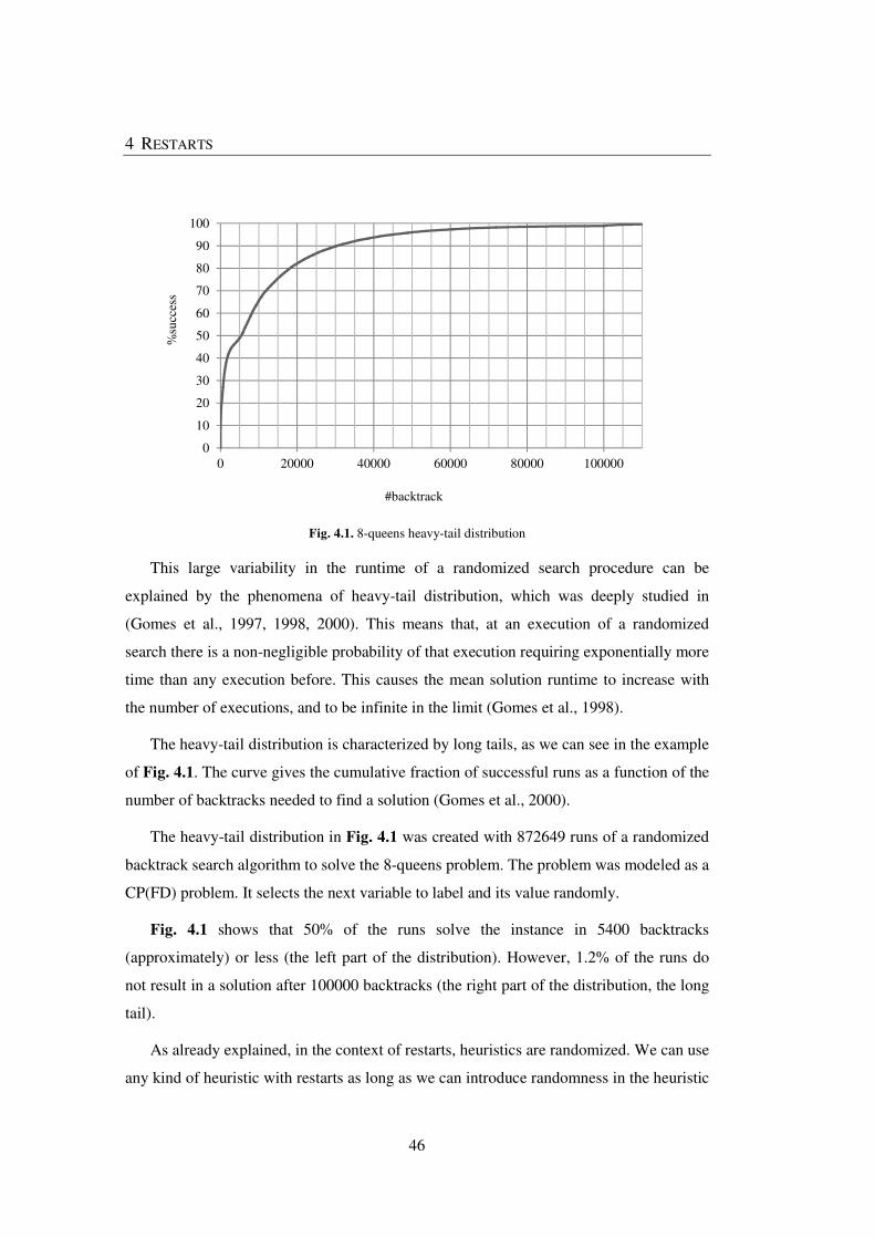
4 RESTARTS
46
Fig. 4.1. 8-queens heavy-tail distribution
This large variability in the runtime of a randomized search procedure can be
explained by the phenomena of heavy-tail distribution, which was deeply studied in
(Gomes et al., 1997, 1998, 2000). This means that, at an execution of a randomized
search there is a non-negligible probability of that execution requiring exponentially more
time than any execution before. This causes the mean solution runtime to increase with
the number of executions, and to be infinite in the limit (Gomes et al., 1998).
The heavy-tail distribution is characterized by long tails, as we can see in the example
of Fig. 4.1. The curve gives the cumulative fraction of successful runs as a function of the
number of backtracks needed to find a solution (Gomes et al., 2000).
The heavy-tail distribution in Fig. 4.1 was created with 872649 runs of a randomized
backtrack search algorithm to solve the 8-queens problem. The problem was modeled as a
CP(FD) problem. It selects the next variable to label and its value randomly.
Fig. 4.1 shows that 50% of the runs solve the instance in 5400 backtracks
(approximately) or less (the left part of the distribution). However, 1.2% of the runs do
not result in a solution after 100000 backtracks (the right part of the distribution, the long
tail).
As already explained, in the context of restarts, heuristics are randomized. We can use
any kind of heuristic with restarts as long as we can introduce randomness in the heuristic
0
10
20
30
40
50
60
70
80
90
100
0 20000 40000 60000 80000 100000
%su
cces
s
#backtrack

4.2 SEARCH RESTART STRATEGIES
47
decision. Also, heuristics, for variable and value selection, have impact in the heavy-tail
distribution (Hulubei and O’Sullivan, 2006). A good combination of variable and value
selection heuristics can even eliminate the heavy-tail behavior from certain classes of
problems. But a poor combination ensures that such behavior is observed.
4.2 SEARCH RESTART STRATEGIES
The use of restarts is really a straightforward technique, which simply restarts the
algorithm when a cutoff value is reached. But being a simple technique does not mean
that different decisions do not have great impact. So, restart strategies are used for
defining the cutoff and for updating it after each restart. A possible restart strategy
consists of defining a cutoff value in the number of backtracks. If a randomized search
algorithm does not find a solution within the cutoff, the run is terminated and the
algorithm is restarted. The algorithm is repeatedly run, each time limiting the maximum
number of backtracks to the cutoff value. In practice, a good cutoff value eliminates the
heavy-tail phenomena, but unfortunately such a value has to be found empirically (Gomes
et al., 1998).
In practice, a simple universal restart strategy can be used. One universal restart
strategy was proposed in (Walsh, 1999), where the cutoff values are systematically
incremented by a geometric factor, which seems to work well in practice. Incrementing
the cutoff makes the algorithm complete, but, for the sake of completeness it is sufficient
to linearly increment the cutoff value by a constant. This simple policy is thus able to
prove unsatisfiability (Baptista and Silva, 2000).
It is possible to define an optimal restart policy (a fixed cutoff value) if the run-time
distribution of the solver is known (Luby et al., 1993). Even if the distribution is not
known, it is possible to define a universal restart policy (a sequence of cutoff values)
ensuring that the expected run-time is within a log factor of the optimal. This universal
restart policy is a sequence of cutoff values in the form 1, 1, 2, 1, 1, 2, 4, 1, 1, 2, 1, 1, 2, 4,
8, 1, 1, 2, 1, 1, 2, 4, 1, 1, 2, 1, 1, 2, 4, 8, 16, 1, 1, … and is known as the Luby restarts
strategy. Also, in (Luby et al., 1993) it is shown that no other restart policies are better by
more than a constant factor.
4 RESTARTS
48
Unfortunately, real world problems violate the assumptions made in (Luby et al.,
1993) about the optimal restart policies (Kautz et al., 2002). It is not just the runtime
distribution that gives evidence about the behavior of the solver. So, (Kautz et al., 2002)
introduce dynamic restart policies, which are restart policies for a randomized algorithm
that take real-time observations about attributes of instances and about solver behavior.
Those dynamic restart policies are based on the state of the solver and on the runtime
distribution. An interesting result is that only a short period of observation is necessary to
accurately find good restart policies.
In (Huang, 2007) the effect of different restart policies in SAT solvers with clause
learning is studied. The results show that the restart policies have impact in the solver
efficiency for real world instances. The important conclusion is the importance of
adapting a strategy to a family of instances, i.e., the importance of using dynamic restart
strategies.
In (Gagliolo and Schmidhuber, 2007), a restart strategy for SAT algorithms is learned
based on the instances solved. This strategy is an interleaving of the Luby universal
strategy (Luby et al., 1993) and a learned fixed cutoff. Due to this interleaving, the
strategy is more robust. However, in (Wu and Beek, 2007) it is argued that the fixed
cutoff learned is not useful in many practical settings. They focus on learning good
universal restart strategies, and show empirically their utility in real word instances of
SAT.
Frequent restarts can improve SAT solvers. But, in some cases, frequent restarts can
be harmful. A dynamic restart strategy is presented in (Biere, 2008) in the context of
conflict driven SAT solvers with learning. It is an adaptive technique that measures the
agility (based on variable flips – flipping the value of a variable means that it is assigned
the opposite value of what was assigned the last time) of the search dynamically, and uses
that information to control the restart frequency. It reduces restarts frequency if the agility
of the SAT solver is high. Experimental results show that this restart strategy improves
the SAT solver. Another dynamic restart strategy is presented in (Ryvchin and Strichman,
2008); it is based on local information, i.e., the strategy applies restarts according to
measures local to each branch. Preliminary results show that for some cases a little
improvement is observed.
4.3 COMPLETENESS
49
Restart strategies are an active research area in SAT algorithms with recent
developments. The use of machine learning techniques to select the best restart strategy
can improve the SAT solver performance (Haim and Walsh, 2009). A recent restart
strategy that defines cutoffs based on the size of conflict clauses outperforms traditional
restart strategies (Pipatsrisawat and Darwiche, 2009a). A different restart strategy uses
heuristics, based on information about different search parameters, to decide whether to
perform a restart or not (Sinz and Iser, 2009). And, in (Pipatsrisawat and Darwiche,
2009b) a worthy of note conclusion states that a frequent restart policy might be a key to
the efficiency of modern solvers.
The use of aggressive strategies of restarts, namely frequent restarts, means that the
solver has less time to reach a complete assignment (solution). The restart could occur too
soon, not allowing the solver to reach a solution. This problem was addressed for SAT,
where the SAT solver can decide to postpone a restart if the search is approaching a
solution (Audemard and Simon, 2012).
In the area of CP(FD), the use of restarts is started to be considered important. Restart
strategies are not an area of active research. Nevertheless, some interesting results exist.
In (Grimes et al., 2009) a simple constraint model is used that combines a generic
adaptive heuristic with naive propagation and restarts. This model often outperforms
state-of-the-art solvers for open job and job shop problems. This example shows the
potential power of restarts, hence, we believe that restart techniques should be an
important research area in CP(FD).
4.3 COMPLETENESS
If restarts are used with a fixed cutoff value, then the resulting algorithm is not complete.
Although the resulting algorithm could have some probability of solving every satisfiable
instance, it may not be able to prove unsatisfiability. A solution to this problem is to
implement a policy for increasing the cutoff value (Walsh, 1999). A simple policy is to
increment by a constant the cutoff value after each restart. The resulting algorithm is
complete, and thus able to prove unsatisfiability (Baptista and Silva, 2000). Observe that
4 RESTARTS
50
this approach resembles iterative deepening, in the sense that more search space is
explored after each restart.
However, the incremental cutoff policy still exhibits a key drawback, because paths in
the search tree can be visited more than once. This was addressed for SAT problems in
(Baptista et al., 2001), where nogoods are recorded from the last branch of the search tree
before the restart (search signature). Those recorded nogoods guarantee that the already
visited search space is not searched again. More recently, the same idea was applied for
CP(FD) (Lecoutre et al., 2007a, 2007b). This is considered a form of learning, since
decisions (nogoods) are learned when the restart occurs and then used in the subsequent
runs. Note that, if the search signature is recorded, no randomization is needed to
guarantee that the next run searches a different search space.
Another approach that guarantees that paths in the search tree cannot be visited more
than once, is proposed in (Mehta et al., 2009). In the context of restarts, the algorithm
avoids visited regions of the search space by extracting them from the unvisited search
space of the problem. This is also a form of learning during search. Empirical results
show that this approach outperforms an algorithm that maintains arc consistency (MAC)
combined with weighted degree heuristic and restarts. Important to notice is the fact that
this approach is a form of learning that does not rely on constraint propagation. Instead, it
relies on a reformulation of the CSP.
4.4 LEARNING FROM RESTARTS
A successful use of nogoods in CP(FD) was presented in (Lecoutre et al., 2007a),
consisting of nogoods recorded from restarts, which are used not to search again the
already visited search tree. Our work is inspired by these nogoods, so we will deeply
explain it.
Consider a search tree built by a backtracking search algorithm with a 2-way
branching scheme. In Fig. 4.2 we can see an example of such a tree just before the restart
occurs. The left branch is called the positive decision and corresponds to an assignment.
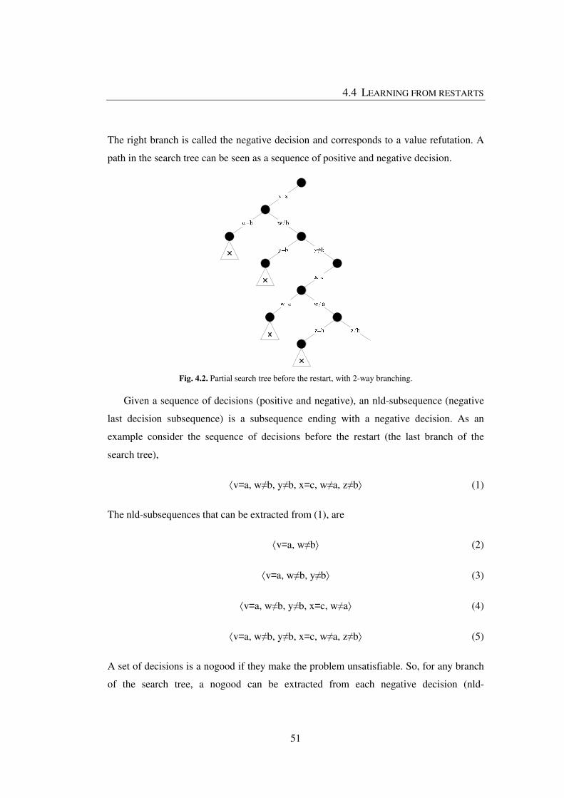
4.4 LEARNING FROM RESTARTS
51
The right branch is called the negative decision and corresponds to a value refutation. A
path in the search tree can be seen as a sequence of positive and negative decision.
Fig. 4.2. Partial search tree before the restart, with 2-way branching.
Given a sequence of decisions (positive and negative), an nld-subsequence (negative
last decision subsequence) is a subsequence ending with a negative decision. As an
example consider the sequence of decisions before the restart (the last branch of the
search tree),
v=a, w≠b, y≠b, x=c, w≠a, z≠b (1)
The nld-subsequences that can be extracted from (1), are
v=a, w≠b (2)
v=a, w≠b, y≠b (3)
v=a, w≠b, y≠b, x=c, w≠a (4)
v=a, w≠b, y≠b, x=c, w≠a, z≠b (5)
A set of decisions is a nogood if they make the problem unsatisfiable. So, for any branch
of the search tree, a nogood can be extracted from each negative decision (nld-
4 RESTARTS
52
subsequence). Consider an nld-subsequence d1, d2, …, di; the set {d1, d2, …, ¬di} is a
nogood (nld-nogood). The nld-nogoods that can be extracted from (1), one for each nld-
subsequence (2-5) are,
{v=a, w=b} (6)
{v=a, w≠b, y=b} (7)
{v=a, w≠b, y≠b, x=c, w=a} (8)
{v=a, w≠b, y≠b, x=c, w≠a, z=b} (9)
As noted in (Lecoutre et al., 2007a) the nld-nogood corresponds to the definition of
generalized nogoods (Katsirelos and Bacchus, 2005), because it contains both positive
and negative decisions. They also show that nld-nogoods can be reduced in size,
considering only positive decisions. Consider an nld-subsequence d1, d2, …, di and
Pos(d1, d2, …, di) denoting the set of positive decisions of the nld-subsequence, then the
set Pos(d1, d2, …, di) ∪ {¬di} is a nogood (reduced nld-nogood) as (10-13) below, for
our example.
{v=a, w=b} (10)
{v=a, y=b} (11)
{v=a, x=c, w=a} (12)
{v=a, x=c, z=b} (13)
The advantages of using a reduced nld-nogood are more pruning power and reduction
in space complexity. Also notice that the set of reduced nld-nogoods is equivalent to its
original set of nld-nogoods. It consists of a more compact and efficient representation of
nogoods.

4.5 RESULTS ON RESTARTS
53
4.5 RESULTS ON RESTARTS
The main focus of our work is the use of restarts in CP(FD), which is a technique that is
starting to be widely used. As learned from the SAT community we know that the
successful use of restarts should include learning and heuristics based on conflicts. So,
our work needs to incorporate all these ideas. But, for now, in this section we will present
our results on using restarts in CP(FD).
First, we will present a preliminary study on restarts, conducted at the beginning of
this research, with the objective of trying to unveil the potential of restarts and associated
techniques. Next we will present a more elaborated study, on harder instances and in the
context of domain-splitting search.
We use domain-splitting because we drive our research to learning from restarts, in
the context of domain-splitting search, because learning is an important piece of the
success of restarts. A good application of restarts and learning in CP(FD) is the work on
recording nogoods from restarts (Lecoutre et al., 2007b, 2007a). So, based on this work,
we have generalized the recording of nogoods from restarts for use in the context of
domain-splitting search. This will be explained in the next chapter, but, for now, we will
present in this chapter only the results related with restarts in domain-splitting search.
4.5.1 Preliminary results
Because restarts are not commonly used in CP(FD), we start by choosing a widely used
problem and show that restarts and associated techniques are useful. We choose the n-
queens problem (Hussain, n.d.), modeled as CP(FD), to conduct the empirical study on
restarts (Baptista and Azevedo, 2010). We use a randomized backtrack search algorithm
with d-ary branching and restarts, implemented in Comet.
We start by trying to unveil the heavy-tail nature of the n-queens problem. The
backtrack search algorithm was configured to choose randomly, at each node, a variable
and its value. This means that we chose rand both for the branching heuristic and for the
value selection heuristic. Different executions of this algorithm can result in extremely
different runtimes exhibiting a heavy-tail distribution (Gomes et al., 2000). Hence, we ran

4 RESTARTS
54
872649 times this algorithm for the 8-queens problem instance (the referred number of
runs is due to computational limitations). If the algorithm can not find a solution within
1000000 backtracks, the execution is aborted. We measure the success by the number of
backtracks needed to find a solution.
After all the runs, the graph in Fig. 4.1 was constructed. The curve gives the
cumulative fraction of successful runs as a function of the number of backtracks, showing
a typical heavy-tail distribution with the long tail. From Fig. 4.1 we can see that 50% of
the runs solve the instances in 5400 backtracks (approximately) or less (the left part of the
distribution). However, 1.2% of the runs do not result in a solution after 100000
backtracks (the right part of the distribution – the long tail).
Because the 8-queens problem instance has a heavy-tail distribution, one can use a
randomized restart strategy to avoid the long tail (Baptista and Azevedo, 2010). In fact,
after restarting a sufficient number of times, the probability of one of the next runs being
one of the 1.2% of runs of the long tail is very low, and the probability of one of the runs
being one of the 50% is high. Therefore we will show that the use of restarts solves the n-
queens problem more efficiently, when comparing to the algorithm without restarts.
To study the use of restarts in the n-queens problem we implement three different
configurations of the backtrack search algorithm:
1. (FF) The backtrack search with the dom fail-first heuristic. We do not use
randomization nor restarts.
2. (FF+Rand) We add randomization to the FF configuration. We select
randomly the next branching variable among the ones with the best heuristic
value.
3. (FF+Rst) We add restarts to the FF+Rand configuration. For the restarts
strategy we use an initial cutoff of 1 and the increment to the cutoff value
after each restart is 10. We use a more aggressive randomization, that
randomly chooses between the variables with the three best values.
In Table 4.1 we present the results of running the three algorithms on different
instances of the n-queens problem. The values in the table represent the number of
backtracks needed to find the solution for the n-queens instance indicated in the first line
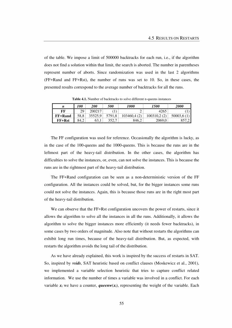
4.5 RESULTS ON RESTARTS
55
of the table. We impose a limit of 500000 backtracks for each run, i.e., if the algorithm
does not find a solution within that limit, the search is aborted. The number in parentheses
represent number of aborts. Since randomization was used in the last 2 algorithms
(FF+Rand and FF+Rst), the number of runs was set to 10. So, in these cases, the
presented results correspond to the average number of backtracks for all the runs.
Table 4.1. Number of backtracks to solve different n-queens instances
n 100 200 500 1000 1500 2000
FF 29 200217 (1) 2 4265 (1) FF+Rand 58,8 35525,9 5791,8 103460,4 (2) 100310,2 (2) 50003,6 (1) FF+Rst 84,2 63,1 352,7 846,2 2069,0 857,2
The FF configuration was used for reference. Occasionally the algorithm is lucky, as
in the case of the 100-queens and the 1000-queens. This is because the runs are in the
leftmost part of the heavy-tail distribution. In the other cases, the algorithm has
difficulties to solve the instances, or, even, can not solve the instances. This is because the
runs are in the rightmost part of the heavy-tail distribution.
The FF+Rand configuration can be seen as a non-deterministic version of the FF
configuration. All the instances could be solved, but, for the bigger instances some runs
could not solve the instances. Again, this is because those runs are in the right most part
of the heavy-tail distribution.
We can observe that the FF+Rst configuration uncovers the power of restarts, since it
allows the algorithm to solve all the instances in all the runs. Additionally, it allows the
algorithm to solve the bigger instances more efficiently (it needs fewer backtracks), in
some cases by two orders of magnitude. Also note that without restarts the algorithms can
exhibit long run times, because of the heavy-tail distribution. But, as expected, with
restarts the algorithm avoids the long tail of the distribution.
As we have already explained, this work is inspired by the success of restarts in SAT.
So, inspired by vsids, SAT heuristic based on conflict clauses (Moskewicz et al., 2001),
we implemented a variable selection heuristic that tries to capture conflict related
information. We use the number of times a variable was involved in a conflict. For each
variable xi we have a counter, queenw(xi), representing the weight of the variable. Each
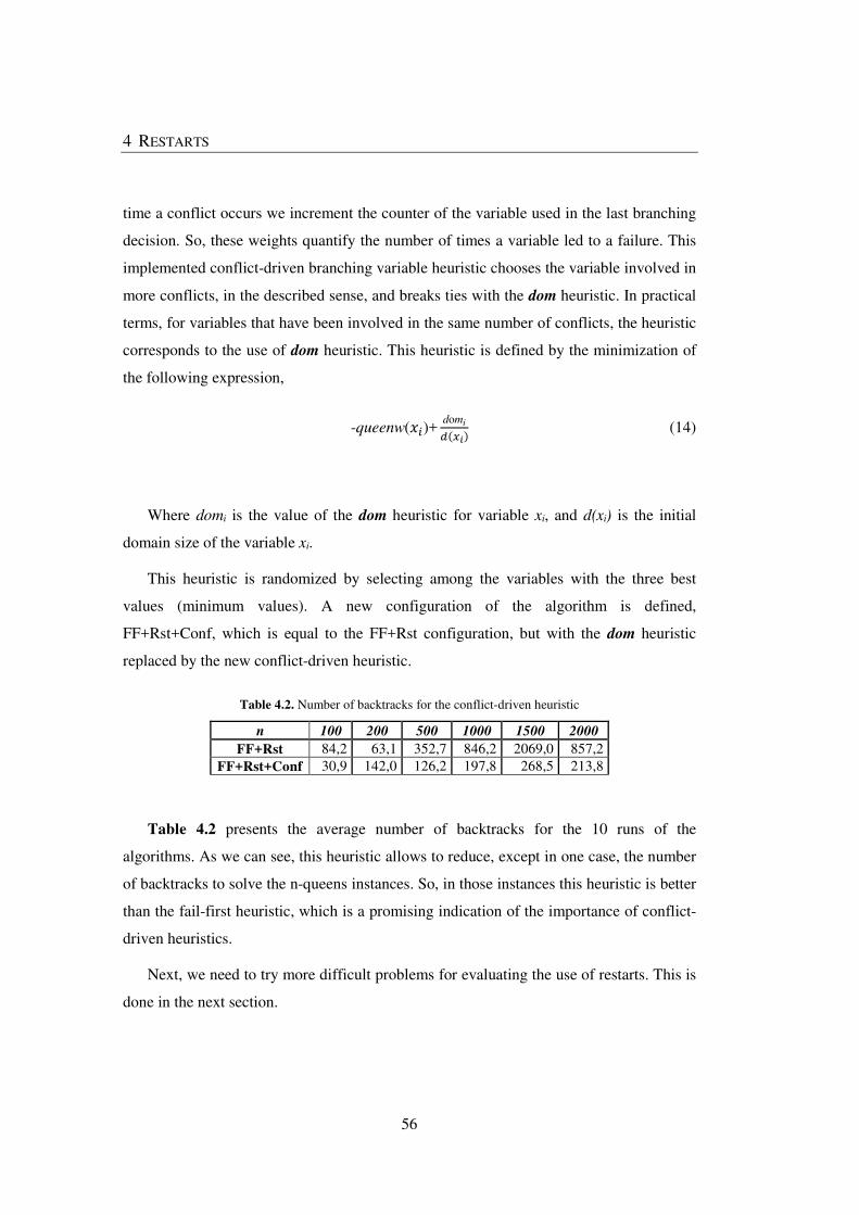
4 RESTARTS
56
time a conflict occurs we increment the counter of the variable used in the last branching
decision. So, these weights quantify the number of times a variable led to a failure. This
implemented conflict-driven branching variable heuristic chooses the variable involved in
more conflicts, in the described sense, and breaks ties with the dom heuristic. In practical
terms, for variables that have been involved in the same number of conflicts, the heuristic
corresponds to the use of dom heuristic. This heuristic is defined by the minimization of
the following expression,
-queenw(�)+ domi
���� (14)
Where domi is the value of the dom heuristic for variable xi, and d(xi) is the initial
domain size of the variable xi.
This heuristic is randomized by selecting among the variables with the three best
values (minimum values). A new configuration of the algorithm is defined,
FF+Rst+Conf, which is equal to the FF+Rst configuration, but with the dom heuristic
replaced by the new conflict-driven heuristic.
Table 4.2. Number of backtracks for the conflict-driven heuristic
n 100 200 500 1000 1500 2000
FF+Rst 84,2 63,1 352,7 846,2 2069,0 857,2 FF+Rst+Conf 30,9 142,0 126,2 197,8 268,5 213,8
Table 4.2 presents the average number of backtracks for the 10 runs of the
algorithms. As we can see, this heuristic allows to reduce, except in one case, the number
of backtracks to solve the n-queens instances. So, in those instances this heuristic is better
than the fail-first heuristic, which is a promising indication of the importance of conflict-
driven heuristics.
Next, we need to try more difficult problems for evaluating the use of restarts. This is
done in the next section.

4.5 RESULTS ON RESTARTS
57
4.5.2 Using Restarts
In our empirical study we use the Comet System, using the constraint programming
solver over finite domains, in a dual core Pentium (E5200) at 2.5 GHz with 2GB of
memory, running a 64 bits Linux system.
We use instances of Talisman squares. A talisman square is a magic square of size n
but with constraints stating that the difference between two adjacent cells must be greater
than some constant, k (see section 2.1.5.2). For each of the instances we run two
randomized backtrack search algorithms, one without restarts and the other with restarts.
Each algorithm is run 100 times for each of the instances.
All the algorithms use domain-splitting search, and a value heuristic that chooses the
splitting value randomly, from the current domain of the variable. To evaluate the
execution of the algorithms we use the number of fails needed to find a solution. If the
algorithms do not find a solution within 100000 fails, the execution is aborted.
The first algorithm, without restarts, uses dom, a variable selection heuristic based on
the fail-first principle, that chooses the variable with the smallest domain, breaking ties
randomly. The second algorithm is equal to the first one plus restarts, but chooses
randomly between the variables with the two best heuristic values. We use a restart
strategy with initial cutoff of 1000 fails and after each restart we increment the cutoff by
5 fails.
We use the dom heuristic because the fail-first principle is still considered to be the
main reason for the success of heuristics on CP(FD); and also because it is a generic and
low overhead heuristic.
Table 4.3 summarizes the results of running the two algorithms on instances of the
talisman square. The first column indicates the instances used, where the first number is
the size n of the talisman and the second number is the minimum difference k between
adjacent cells. The next columns define, respectively, for each algorithm, the average
number of fails, the average runtime, in milliseconds, and the number of runs aborted.
When computing the average runtime and average fails, the aborted runs are included.
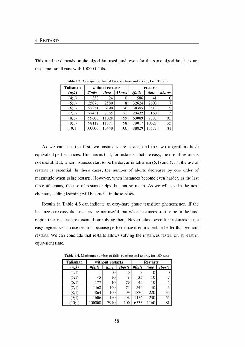
4 RESTARTS
58
This runtime depends on the algorithm used, and, even for the same algorithm, it is not
the same for all runs with 100000 fails.
Table 4.3. Average number of fails, runtime and aborts, for 100 runs
Talisman without restarts restarts
(n;k) #fails time Aborts #fails time aborts
(4;1) 333 24 0 586 41 0 (5;1) 35076 2580 8 32624 2608 7 (6;1) 82851 6890 76 38395 3518 5 (7;1) 77451 7355 71 29432 3160 3 (8;1) 99008 11028 99 63089 7885 35 (9;1) 98112 11871 98 79017 10623 55
(10;1) 100000 13440 100 88829 13577 81
As we can see, the first two instances are easier, and the two algorithms have
equivalent performances. This means that, for instances that are easy, the use of restarts is
not useful. But, when instances start to be harder, as in talisman (6;1) and (7;1), the use of
restarts is essential. In these cases, the number of aborts decreases by one order of
magnitude when using restarts. However, when instances become even harder, as the last
three talismans, the use of restarts helps, but not so much. As we will see in the next
chapters, adding learning will be crucial in those cases.
Results in Table 4.3 can indicate an easy-hard phase transition phenomenon. If the
instances are easy then restarts are not useful, but when instances start to be in the hard
region then restarts are essential for solving them. Nevertheless, even for instances in the
easy region, we can use restarts, because performance is equivalent, or better than without
restarts. We can conclude that restarts allows solving the instances faster, or, at least in
equivalent time.
Table 4.4. Minimum number of fails, runtime and aborts, for 100 runs
Talisman without restarts Restarts
(n;k) #fails time aborts #fails time aborts
(4;1) 1 0 0 3 0 0 (5;1) 45 10 8 35 10 7 (6;1) 177 20 76 43 10 5 (7;1) 1462 100 71 344 40 3 (8;1) 864 100 99 1830 220 35 (9;1) 1606 160 98 1156 230 55
(10;1) 100000 7910 100 6333 1160 81
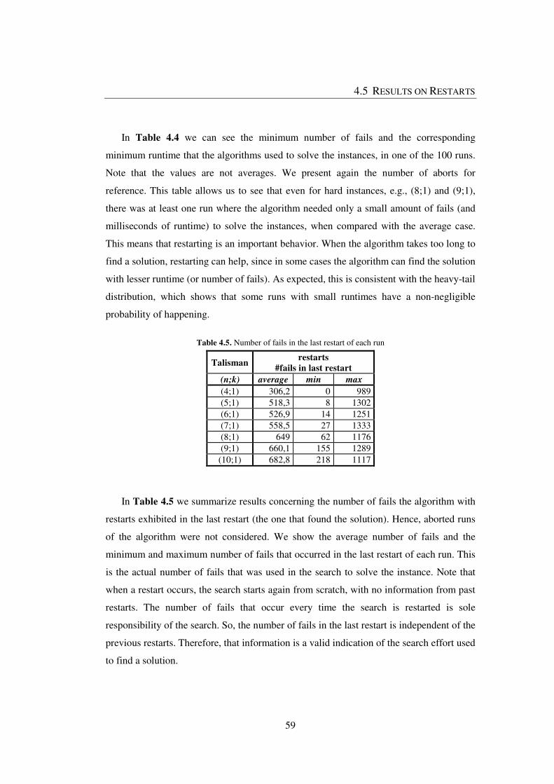
4.5 RESULTS ON RESTARTS
59
In Table 4.4 we can see the minimum number of fails and the corresponding
minimum runtime that the algorithms used to solve the instances, in one of the 100 runs.
Note that the values are not averages. We present again the number of aborts for
reference. This table allows us to see that even for hard instances, e.g., (8;1) and (9;1),
there was at least one run where the algorithm needed only a small amount of fails (and
milliseconds of runtime) to solve the instances, when compared with the average case.
This means that restarting is an important behavior. When the algorithm takes too long to
find a solution, restarting can help, since in some cases the algorithm can find the solution
with lesser runtime (or number of fails). As expected, this is consistent with the heavy-tail
distribution, which shows that some runs with small runtimes have a non-negligible
probability of happening.
Table 4.5. Number of fails in the last restart of each run
Talisman restarts
#fails in last restart
(n;k) average min max
(4;1) 306,2 0 989 (5;1) 518,3 8 1302 (6;1) 526,9 14 1251 (7;1) 558,5 27 1333 (8;1) 649 62 1176 (9;1) 660,1 155 1289
(10;1) 682,8 218 1117
In Table 4.5 we summarize results concerning the number of fails the algorithm with
restarts exhibited in the last restart (the one that found the solution). Hence, aborted runs
of the algorithm were not considered. We show the average number of fails and the
minimum and maximum number of fails that occurred in the last restart of each run. This
is the actual number of fails that was used in the search to solve the instance. Note that
when a restart occurs, the search starts again from scratch, with no information from past
restarts. The number of fails that occur every time the search is restarted is sole
responsibility of the search. So, the number of fails in the last restart is independent of the
previous restarts. Therefore, that information is a valid indication of the search effort used
to find a solution.
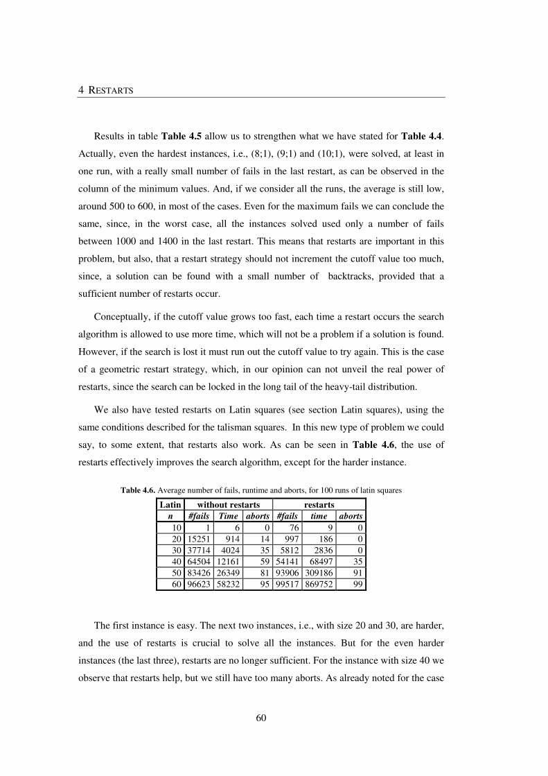
4 RESTARTS
60
Results in table Table 4.5 allow us to strengthen what we have stated for Table 4.4.
Actually, even the hardest instances, i.e., (8;1), (9;1) and (10;1), were solved, at least in
one run, with a really small number of fails in the last restart, as can be observed in the
column of the minimum values. And, if we consider all the runs, the average is still low,
around 500 to 600, in most of the cases. Even for the maximum fails we can conclude the
same, since, in the worst case, all the instances solved used only a number of fails
between 1000 and 1400 in the last restart. This means that restarts are important in this
problem, but also, that a restart strategy should not increment the cutoff value too much,
since, a solution can be found with a small number of backtracks, provided that a
sufficient number of restarts occur.
Conceptually, if the cutoff value grows too fast, each time a restart occurs the search
algorithm is allowed to use more time, which will not be a problem if a solution is found.
However, if the search is lost it must run out the cutoff value to try again. This is the case
of a geometric restart strategy, which, in our opinion can not unveil the real power of
restarts, since the search can be locked in the long tail of the heavy-tail distribution.
We also have tested restarts on Latin squares (see section Latin squares), using the
same conditions described for the talisman squares. In this new type of problem we could
say, to some extent, that restarts also work. As can be seen in Table 4.6, the use of
restarts effectively improves the search algorithm, except for the harder instance.
Table 4.6. Average number of fails, runtime and aborts, for 100 runs of latin squares
Latin without restarts restarts
n #fails Time aborts #fails time aborts
10 1 6 0 76 9 0 20 15251 914 14 997 186 0 30 37714 4024 35 5812 2836 0 40 64504 12161 59 54141 68497 35 50 83426 26349 81 93906 309186 91 60 96623 58232 95 99517 869752 99
The first instance is easy. The next two instances, i.e., with size 20 and 30, are harder,
and the use of restarts is crucial to solve all the instances. But for the even harder
instances (the last three), restarts are no longer sufficient. For the instance with size 40 we
observe that restarts help, but we still have too many aborts. As already noted for the case
4.5 RESULTS ON RESTARTS
61
of the Talisman squares, when instances start to be harder, we need something more to
help the restarts strategy. This will be the use of learning that we will see in the next
chapters.
4.5.3 Difficulties on using restarts
Before the results we present in this chapter, we have tested other instances from CSPLib
(Jefferson et al., 1999), Golfers, Quasigroup with Holes and Prime Queen (see sections
2.1.5.4, 2.1.5.3 and 2.1.5.5, respectively), trying to uncover the power of restarts in the
context of domain splitting search. But we ended up in dead ends, because we could not
find good results when restarts alone are applied. For Quasigroups with Holes and Prime
Queen problems all the instances were too hard for the algorithm without restarts and
with restarts. So, the use of restarts was indifferent, since in neither case the algorithm
could find a solution.
For the Golfers problem instances, results are shown in Table 4.7. We ran 20 times
each instance. We have tested other restart strategies, but without improvements on the
results presented. As we can see, the use of restarts does not help the algorithm. Only in
some particular cases we see that restarts help, e.g., golfers (9,4,8) and (10,4,8). But in the
majority of cases we do not see differences in the algorithm with and without restarts.
Still, we can always use restarts, since, for the instances that have solutions, the use of
restarts does not harm the algorithm. On the contrary, for some instances, the use of
restarts, found the solution with fewer fails, e.g., golfers (6,3,7) and (6,4,5).

4 RESTARTS
62
Table 4.7. Using restarts on Golfers
Restart: 0;0 200;+10
(g,s,w) #fails aborts #fails aborts
(6,3,5) 52,2 0 30,3 0 (6,3,6) 363,7 0 220,9 0 (6,3,7) 54061,8 0 20384,0 0 (6,3,8) 4881811,6 19 4999020,0 20 (6,4,5) 17069,3 0 6915,7 0 (6,4,6) 5000000,0 20 4999020,0 20 (6,4,7) 5000000,0 20 4999020,0 20 (6,4,8) 5000000,0 20 4999020,0 20 (7,4,8) 5000000,0 20 4999020,0 20 (8,4,8) 5000000,0 20 4999020,0 20 (9,4,8) 3790771,9 14 3565509,9 7
(10,4,8) 1825628,9 5 1050161,1 0 (5,4,4) 1198,2 0 713,5 0
(6,2,11) 62,1 0 56,5 0 (6,3,5) 35,5 0 56,1 0 (6,4,3) 42,7 0 102,4 0
(7,2,13) 95,1 0 95,7 0 (7,3,4) 3,8 0 5,0 0 (7,4,3) 70,0 0 85,5 0 (7,5,2) 522395,4 2 140,9 0 (8,3,5) 33,5 0 33,9 0 (8,4,9) 5000000,0 20 4999020,0 20 (8,5,2) 2531,3 0 46,5 0
We also tried to use restarts on a real world problem related with cattle nutrition (see
section 2.1.5.6), but we found that the problem was indeed easier than what we expected,
because it could be easily solved without restarts. So, restarts do not have space for
improvements. We tried this problem, because it was a real problem that we face, and had
variables with larger domain sizes, which should be good for domain-splitting search.
4.6 SUMMARY AND FINAL REMARKS
Restarts are widely used in SAT search algorithms and are considered of central
importance. The use of frequent restarts in SAT is considered to be state-of-the-art, which
means that current solvers restart very often, never allowing the search to be lost in the
combinatorial explosion. Of course, restarts in SAT are associated with other important
4.6 SUMMARY AND FINAL REMARKS
63
techniques, namely clause recording, which allows learning in the following restarts. It
was the interplay of these two techniques that allowed the performance boost of SAT
algorithms about seventeen year ago.
Unfortunately, the use of restarts in CP(FD) was normally confined to geometric
restart strategies, which we believe could be one of the reasons why restarts never proved
to be of central importance in CP(FD). We believe that CP(FD) could also benefit with
restarts when we are able to assemble rapid restarts and learning (nogoods recording).
We found empirical evidences that CP(FD) could benefit from rapid restarts. Still, we
found many difficulties in applying restarts per se to CP(FD). After the results presented
in this chapter we focus our research on learning (nogood recording). As we known from
SAT, the joint use of learning, restarts and heuristics based on conflicts is very important
for the success of backtrack search algorithms (Moskewicz et al., 2001). Unfortunately,
learning is not widely used in CP(FD). Yet, some good examples exist, as is the case of
recording nogoods from restarts (Lecoutre et al., 2007b, 2007a). So, inspired by this work
we propose nogoods from restarts in the context of domain splitting search. And then,
using the information within these nogoods we propose a novel kind of variable selection
heuristics. The next chapters will explain and evaluate our proposed nogoods and
heuristics.

65
5 DOMAIN-SPLITTING NOGOODS
We present a generalization of the work presented in (Lecoutre et al., 2007a) about
nogood recording from restarts, in the context of backtrack search algorithms with 2-way
branching. In (Baptista and Azevedo, 2011), using a backtrack search algorithm with
domain-splitting branching, and adapting the concepts described in (Lecoutre et al.,
2007a), a nogood recorded from a restart uses domain splitting decisions instead of
assignment decisions.
In this chapter we present Domain-Splitting (ds) nogoods and Domain-Splitting
Generalized (dsg), as described in (Baptista and Azevedo, 2011), but now using a more
formal description, and extend the work with a space complexity analysis.
Recall that we use finite domains. Consider a search tree built by a backtrack search
algorithm with a domain splitting branching scheme. As for the 2-way branching scheme,
this is also a binary tree. But now the domain is split lexicographically cutting it in one of
its values. In Fig. 5.1 we can see an example of such a tree before the restart occurs.
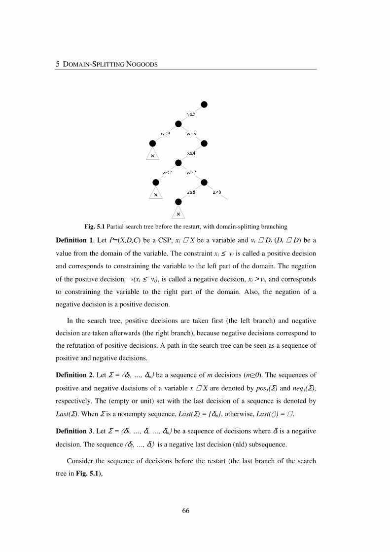
5 DOMAIN-SPLITTING NOGOODS
66
Fig. 5.1 Partial search tree before the restart, with domain-splitting branching
Definition 1. Let P=(X,D,C) be a CSP, xi ∈ X be a variable and vi ∈ Di (Di ∈ D) be a
value from the domain of the variable. The constraint xi ≤ vi is called a positive decision
and corresponds to constraining the variable to the left part of the domain. The negation
of the positive decision, ¬(xi ≤ vi), is called a negative decision, xi > vi, and corresponds
to constraining the variable to the right part of the domain. Also, the negation of a
negative decision is a positive decision.
In the search tree, positive decisions are taken first (the left branch) and negative
decision are taken afterwards (the right branch), because negative decisions correspond to
the refutation of positive decisions. A path in the search tree can be seen as a sequence of
positive and negative decisions.
Definition 2. Let Σ = δ1, …, δm be a sequence of m decisions (m≥0). The sequences of
positive and negative decisions of a variable x ∈ X are denoted by posx(Σ) and negx(Σ),
respectively. The (empty or unit) set with the last decision of a sequence is denoted by
Last(Σ). When Σ is a nonempty sequence, Last(Σ) = {δm}, otherwise, Last() = ∅.
Definition 3. Let Σ = δ1, …, δi, …, δm be a sequence of decisions where δi is a negative
decision. The sequence δ1, …, δi is a negative last decision (nld) subsequence.
Consider the sequence of decisions before the restart (the last branch of the search
tree in Fig. 5.1),
4.6 SUMMARY AND FINAL REMARKS
67
v≤5, w>3, x≤4, w>7, z>6 (15)
The three nld-subsequences from (15) are:
v≤5, w>3 (16)
v≤5, w>3, x≤4, w>7 (17)
v≤5, w>3, x≤4, w>7, z>6 (18)
Proposition 1. Let P be a CSP, Σ = δ1, …, δi be an nld-subsequence of decisions taken
along a branch of the search tree, and Σ’ = δ1, …, ¬δi be a sequence derived from Σ
where the last decision is negated (converted to a positive decision). The set created with
all decisions of Σ’, ∆ = {δ1, …, ¬δi}, is a nogood, called domain-splitting nogood (ds-
nogood).
Proof. In the search tree, positive decisions are taken first, so, if a negative decision (δi)
appears, then the subtree corresponding to the positive decision (¬δi) was refuted.
So, for each nld-subsequence, extracted from (15), we have a ds-nogood,
{v≤5, w≤3} (19)
{v≤5, w>3, x≤4, w≤7} (20)
{v≤5, w>3, x≤4, w>7, z≤6} (21)
In the context of ds-nogoods, a decision node splits the domain in two sets. Also, in
the context of nld-nogoods, as described in (Lecoutre et al., 2007a), a decision node can
be seen also as splitting the domain in two sets: in the positive decision branch the set has
only one value, because of the assignment; and in the negative branch the set has the
other values, because of the refutation of the value. In this sense we can say that ds-
nogoods are more powerful than nld-nogoods, because they use a more compact
representation, since one positive decision can represent more than one value.
5 DOMAIN-SPLITTING NOGOODS
68
Similarly to reduced nld-nogoods (Lecoutre et al., 2007a), we can also have reduced
ds-nogoods, considering only positive decisions,
{v≤5, w≤3} (22)
{v≤5, x≤4, w≤7} (23)
{v≤5, x≤4, z≤6} (24)
As explained in (Baptista and Azevedo, 2011) (reduced) ds-nogoods have potentially
more pruning power than (reduced) nld-nogoods, because they use a more compact
representation, since one decision can represent more than one decision of the nld-
nogoods.
5.1 SIMPLIFYING DS-NOGOODS
By construction, a CSP nogood does not contain two opposite decisions, e.g., y≤4 and
y>4. But a ds-nogood can have more than one decision on the same variable. So, for each
ds-nogood (including the reduced version) a subsumption procedure must be applied to
remove redundant decisions and thus simplify the nogood.
Proposition 2. Let P be a CSP, ∆ = {δ1, …, δi} be a ds-nogood and Σ’ = δ1, …, δi be the
sequence of decisions that created ∆. The ds-nogood ∆ can be simplified in an equivalent
ds-nogood ∆’ = ∪x∈X (Last(posx(Σ’) ∪ Last(neg x(Σ’)). And the reduced version of ∆ can
be simplified in an equivalent reduced ds-nogood ∆’’ = ∪x∈X Last(posx(Σ’).
Proof. As already noted, by construction, nogoods do not contain two opposite decisions.
A decision in the search tree will narrow the domain of a variable, decreasing the upper
bound (a positive decision), or increasing the lower bound (a negative decision).
Subsequent decisions on the same variable will further narrow the domain; hence, it
suffices to maintain, for each variable, only the last positive and last negative decision,
and safely remove the other decision. In the case of reduced ds-nogoods, only the last
(positive) decision has to be kept (for each of its variables).
5.1 SIMPLIFYING DS-NOGOODS
69
Consider again the ds-nogoods (19-21) of our example and the decisions over
variable w in the ds-nogood {v≤5, w>3, x≤4, w>7, z≤6} (21), w>3 and w>7. It is easy to
see, that the decision w>7 subsumes w>3; because decision w>7 is made after w>3 we
can safely remove decision w>3, resulting in a new simplified ds-nogood, {v≤5, x≤4,
w>7, z≤6}. Thus, a great compaction can be obtained with simplified ds-nogoods.
The other two ds-nogoods of our example could not be more simplified, because they
do not include more than one positive/negative decision over the same variable. Consider
the ds-nogood {v≤5, w>3, x≤4, w≤7}, that has two decisions on the same variable, but one
is a positive and the other is a negative decision, hence, no simplification is possible. For
the other ds-nogood, {v≤5, w≤3} no doubt exists, since all decision are over distinct
variables. So, the simplified version of the ds-nogoods (19-21) of our example, are the
following.
{v≤5, w≤3} (25)
{v≤5, w>3, x≤4, w≤7} (26)
{v≤5, x≤4, w>7, z≤6} (27)
Proposition 3. Let P be a CSP, n the number of variables and ∆ be a simplified ds-
nogood. The maximum number of decisions a ds-nogood can have is 2n.
Proof. By definition, a ds-nogood contains decisions. The decisions can be of 2 types, the
positive and the negative decisions. And, from Proposition 2, we know that the simplified
version of ds-nogoods only have, for each of the possible n variables, at most 2 decisions,
one positive and another negative, hence 2n decisions, at most.
Proposition 4. Let P be a CSP, n the number of variables, d the size of the domains, and
Σ be the sequence of decisions taken along a branch of the search tree. The space
complexity to record all the simplified ds-nogoods of Σ is Ο(n2d). The space complexity
to record all the simplified reduced ds-nogoods of Σ is also Ο(n2d).
Proof. The number of negative decisions in any branch is Ο(nd). For each negative
decision a ds-nogood (or a reduced version) is extracted. From Propositions 1 and 2, we
5 DOMAIN-SPLITTING NOGOODS
70
know that the size of any ds-nogood or any reduced ds-nogood is Ο(n), because a
simplified ds-nogood only has, for each variable, the last positive (if any) and the last
negative (if any) decisions. So, the resulting space complexity is Ο(n2d).
So, at each restart, the space complexity to record all the simplified ds-nogoods from
the last branch of the search tree is O(n2d).
5.2 GENERALIZING TO DSG-NOGOODS
Ds-nogoods suffer from a possible key drawback; domain-splitting branching uses
lexicographic order, which limits the expressive power of the search and, consequently,
the learned nogoods. Namely, values are split in two sets lexicographically. It would be
better, for the sake of search flexibility, if the values could be split in any order.
We now assume a broad definition of domain-splitting branching scheme, which
splits the domain D in two disjoint sets, S1 and S2 (i.e. D = S1 ∪ S2 ∧ S1 ∩ S2 = ∅), not
necessarily in lexicographic order. The positive decision considers set S1 as the domain,
in the left branch. If this fails, the negative decision considers set S2 as the domain, in the
right branch. More formally, for a variable x, the left branch corresponds to adding the
constraint x∈S1, and the right branch to adding the constraint x∈S2 (the negative decision
is x∉S1 which is the same as x∈S2). The construction of nogoods applies trivially to this
more generic case, and we call these dsg-nogoods (domain-splitting generalized nogoods)
and reduced dsg-nogoods. The simplified process previously described also applies
trivially to dsg-nogoods and to the reduced version.
Note that (reduced) nld-nogoods (Lecoutre et al., 2007a) are a particular case of
(reduced) dsg-nogoods, since we can simulate 2-way branching with this broad definition
of domain-splitting. The assignment branch corresponds to a set with only one element,
the value of the assignment. The refutation branch corresponds to a set with the remaining
values of the domain.
Recent developments have shown the importance of backtrack search algorithms
using set branching schemes (Balafoutis et al., 2010; Kitching and Bacchus, 2009). The
use of restarts and dsg-nogoods (and the reduced version) in those algorithms is direct if
5.3 POSTING DS-NOGOODS
71
we only have two sets. But even if we have more than two sets, we can use a 2-way style
set branching (Balafoutis et al., 2010), where the sets are tried in a series of binary
choices. The positive decision considers one of the sets as the domain; if this fails, the
negative decision considers the removal of that set from the domain. The use of dsg-
nogoods is thus direct.
5.3 POSTING DS-NOGOODS
When ds-nogoods are extracted from the last branch of the search tree, before the restart,
they could be posted as constraints in the solver. Doing this will avoid the exploration of
the already searched tree. We implement the ds-nogoods using the constraint
programming solver module of the Comet System (Hentenryck and Michel, 2005). Since
Comet does not have nogoods, we had to implement our ds-nogoods on top of Comet.
We created data structures for registering the domain splitting decisions and for creating
and maintaining the nogoods.
After having extracted the ds-nogoods from the last branch of the search tree we
could post the ds-nogoods in the solver’s constraint database. A ds-nogood is a set of
decisions that, if all posted in the constraint solver, originate a conflict. The ds-nogood
can be viewed as a conjunction of those decisions. Consider the simplified version of the
ds-nogoods from our example (25-27); the corresponding conjunctions of decisions are,
(v≤5 ˄ w≤3) (28)
(v≤5 ˄ w>3 ˄ x≤4 ˄ w≤7) (29)
(v≤5 ˄ x≤4 ˄ w>7 ˄ z≤6) (30)
In order to guarantee that these decisions are not satisfied (because otherwise they
would, invariably, conduct the search to a conflict), we must post their negations in the
solver. So, the corresponding constraints must be posted,
(v>5 ˅ w>3) (31)
5 DOMAIN-SPLITTING NOGOODS
72
(v>5 ˅ w≤3 ˅ x>4 ˅ w>7) (32)
(v>5 ˅ x>4 ˅ w≤7 ˅ z>6) (33)
These constraints can be seen as conflict clauses in SAT. They act as a protection for
the failure. The solver will maintain the constraint satisfied, hence, avoiding the set of
decisions originating the failure. This way the search will not repeat search trees from
past restarts. Aimed at simplicity we will generically call the posting of these constraints
as nogood recording.
Theoretically, recording the ds-nogoods from the last branch of the search tree will
help the search, since it will avoid making the same bad decisions, i.e., exploring the
already explored failed subtree. However, when trying to do this we were unable to show
the usefulness of using ds-nogoods.
Indeed, in all the empirical evaluation conducted we did not observe improvements in
the search algorithm with ds-nogoods. We have tried to use ds-nogoods to improve the
algorithm to solve different CP(FD) problems instances, but we found various dead ends.
Posting all nogoods, or only small size nogoods, results in no relevant improvements.
And, we have noticed that, when setting the algorithm to record only small nogoods, the
number of recorded nogoods is very low, which could indicate that the majority of the
nogoods extracted from restarts are of big sizes.
The importance of using only small nogoods is related with space limitation and
pruning power. Small nogoods are better than large ones, since small nogoods are more
generic, and could be more effective in reducing the search space. On the other hand, big
nogoods are more difficult to apply, due to the large number of decisions that must occur
simultaneously.
Because of the very nature of domain-splitting search, the first decisions will
primarily narrow variable domains. In fact, before a variable can be assigned a value, its
domain must be narrowed by successive decisions.
Due to this, when a restart occurs, the last branch of the search tree will have, in the
beginning (at least in the beginning this effect is more problematic/common) or spread
through this last branch, many decisions that only reduce the variable domains. We could
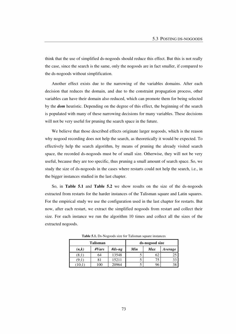
5.3 POSTING DS-NOGOODS
73
think that the use of simplified ds-nogoods should reduce this effect. But this is not really
the case, since the search is the same, only the nogoods are in fact smaller, if compared to
the ds-nogoods without simplification.
Another effect exists due to the narrowing of the variables domains. After each
decision that reduces the domain, and due to the constraint propagation process, other
variables can have their domain also reduced, which can promote them for being selected
by the dom heuristic. Depending on the degree of this effect, the beginning of the search
is populated with many of these narrowing decisions for many variables. These decisions
will not be very useful for pruning the search space in the future.
We believe that those described effects originate larger nogoods, which is the reason
why nogood recording does not help the search, as theoretically it would be expected. To
effectively help the search algorithm, by means of pruning the already visited search
space, the recorded ds-nogoods must be of small size. Otherwise, they will not be very
useful, because they are too specific, thus pruning a small amount of search space. So, we
study the size of ds-nogoods in the cases where restarts could not help the search, i.e., in
the bigger instances studied in the last chapter.
So, in Table 5.1 and Table 5.2 we show results on the size of the ds-nogoods
extracted from restarts for the harder instances of the Talisman square and Latin squares.
For the empirical study we use the configuration used in the last chapter for restarts. But
now, after each restart, we extract the simplified nogoods from restart and collect their
size. For each instance we run the algorithm 10 times and collect all the sizes of the
extracted nogoods.
Table 5.1. Ds-Nogoods size for Talisman square instances
Talisman ds-nogood size
(n,k) #Vars #ds-ng Min Max Average
(8;1) 64 13548 5 62 25 (9;1) 81 15211 5 75 33
(10;1) 100 20964 5 96 38

5 DOMAIN-SPLITTING NOGOODS
74
Table 5.2. Ds-Nogoods size for Latin square instances
Latin ds-nogood size
n #Vars #ds-ng Min Max Average
40 1600 568 607 1444 1366 50 2500 5084 468 2291 2158 60 3600 13332 950 3344 3143
The tables are organized as follow. The first column is the instance considered, the
second one is the number of decision variables used in the CP(FD) model and the third
column identifies the number of ds-nogoods recorded. The last three columns are,
respectively, the size of the smallest nogood, the size of the largest nogood and the
average size of all nogoods.
First note that all the maximum sizes of ds-nogoods are below the maximum value of
2 times the number of variables (Proposition 3). From Table 5.1 we can see that small
nogoods indeed exist. For all instances, the smallest nogood has only 5 decisions. But, on
average, the size of nogoods is not so small, from 25 to 38, and the maximum is at least
the double of the average. And if we look at Table 5.2 even the smallest nogood is too
big. Also note that the average is very near the maximum size, which means that the
majority of nogoods have a large size.
Fig. 5.2 Distribution of ds-nogoods sizes for Talisman squares
0
100
200
300
400
500
600
700
0 10 20 30 40 50 60 70 80 90 100
T-(8;1)
T-(9;1)
T-(10;1)
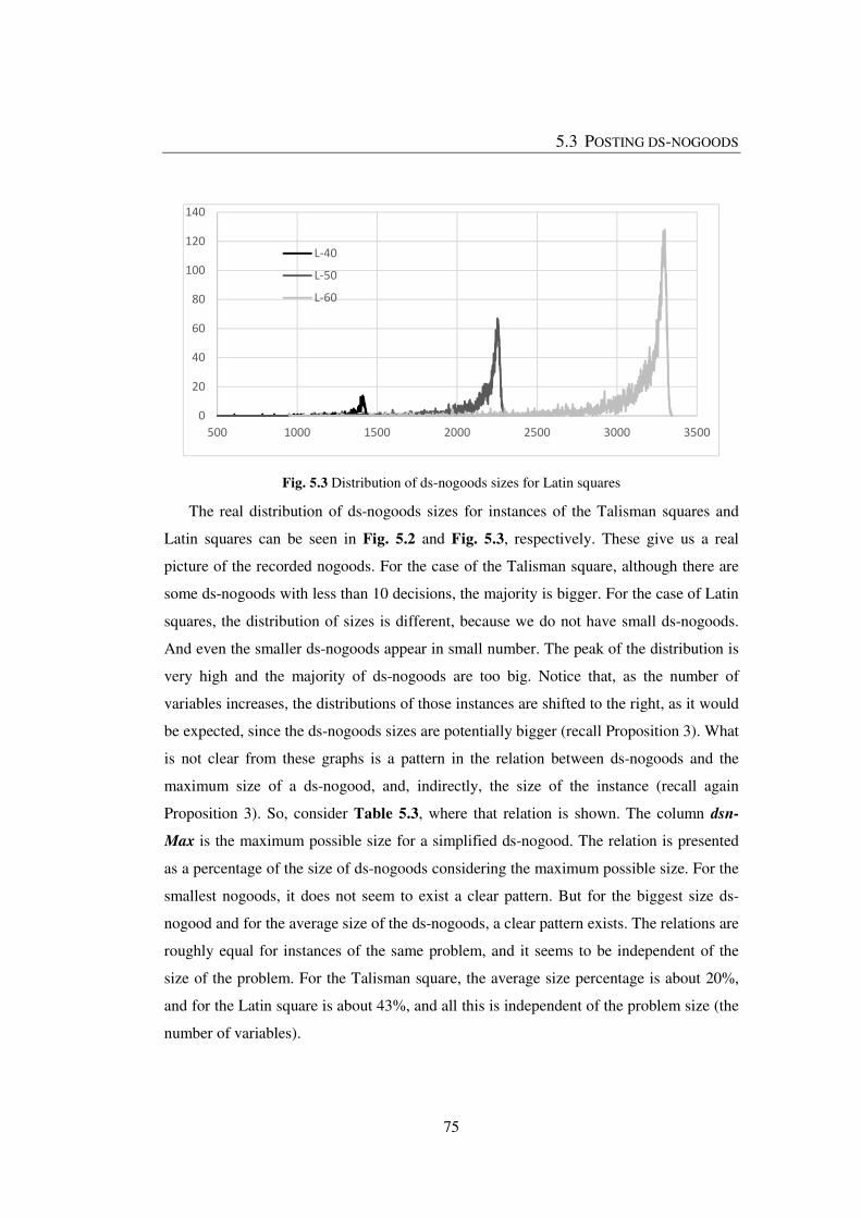
5.3 POSTING DS-NOGOODS
75
Fig. 5.3 Distribution of ds-nogoods sizes for Latin squares
The real distribution of ds-nogoods sizes for instances of the Talisman squares and
Latin squares can be seen in Fig. 5.2 and Fig. 5.3, respectively. These give us a real
picture of the recorded nogoods. For the case of the Talisman square, although there are
some ds-nogoods with less than 10 decisions, the majority is bigger. For the case of Latin
squares, the distribution of sizes is different, because we do not have small ds-nogoods.
And even the smaller ds-nogoods appear in small number. The peak of the distribution is
very high and the majority of ds-nogoods are too big. Notice that, as the number of
variables increases, the distributions of those instances are shifted to the right, as it would
be expected, since the ds-nogoods sizes are potentially bigger (recall Proposition 3). What
is not clear from these graphs is a pattern in the relation between ds-nogoods and the
maximum size of a ds-nogood, and, indirectly, the size of the instance (recall again
Proposition 3). So, consider Table 5.3, where that relation is shown. The column dsn-
Max is the maximum possible size for a simplified ds-nogood. The relation is presented
as a percentage of the size of ds-nogoods considering the maximum possible size. For the
smallest nogoods, it does not seem to exist a clear pattern. But for the biggest size ds-
nogood and for the average size of the ds-nogoods, a clear pattern exists. The relations are
roughly equal for instances of the same problem, and it seems to be independent of the
size of the problem. For the Talisman square, the average size percentage is about 20%,
and for the Latin square is about 43%, and all this is independent of the problem size (the
number of variables).
0
20
40
60
80
100
120
140
500 1000 1500 2000 2500 3000 3500
L-40
L-50
L-60

5 DOMAIN-SPLITTING NOGOODS
76
We could not say if those patterns denote something or some characteristic. But we
can say that they are consistent with the observation of bigger ds-nogoods existence,
since, as the instance size grows, the size of nogoods also grows. And also, that they are
independent of the size of the problem instance; so, for different instances of the same
problem, one should expect the same behavior of ds-nogood recording, i.e., larger ds-
nogoods without effective pruning power.
Table 5.3. Relation between ds-nogoods sizes and maximum size
Instances ds-nogood size
(n,k) #Vars dsn-MAX Min Max Average
T-(8;1) 64 128 5 4% 62 48% 25 20%
T-(9;1) 81 162 5 3% 75 46% 33 20%
T-(10;1) 100 200 5 3% 96 48% 38 19%
L-40 1600 3200 607 19% 1444 45% 1366 43%
L-50 2500 5000 468 9% 2291 46% 2158 43%
L-60 3600 7200 950 13% 3344 46% 3143 44%
In spite of the lack of pruning power of the ds-nogoods extracted from the last branch
of the search tree before the restarts, ds-nogoods can still be used. As already explained,
one of the key factors of a successful restarts implementation is the use of a heuristic
based on nogoods. In SAT, the vsids heuristic is based on the occurrence of literals in
conflict clauses.
We have tried to use information related with ds-nogoods in the branching variable
heuristic. Indeed, we have found a way of using information from ds-nogoods in the
heuristic. In the next chapter we will present and evaluate this new branching variable
heuristic that uses information related with the occurrence of variables in ds-nogoods,
which allows solving some instances more efficiently.
5.4 SUMMARY AND FINAL REMARKS
In the context of domain splitting search, we propose to extract from the last branch of the
search tree before the restart occurs, a set of nogoods, that we call domain splitting

5.4 SUMMARY AND FINAL REMARKS
77
nogoods. These ds-nogoods have decisions that can be safely removed; so, in practice, we
use the simplified version of ds-nogoods.
Typically, these nogoods are posted in the search algorithm as constraints
guaranteeing that the already searched space is not searched again. From our experiments
we could not verify the usefulness of using these nogoods in this way. We gave evidences
of why those nogoods are not very useful in practice. This is related with the size of ds-
nogoods. Indeed, ds-nogoods are very big, and so, very specific, which, in practice, make
their application during search very rare.
Nevertheless, our ds-nogoods have valid information, which explain why the already
visited search space had failed. Hence, we could use that information to help the search
algorithm, as we will see in the next chapter.

79
6 USING DS-NOGOODS IN HEURISTICS
Although nogoods are starting to be used in CP(FD), the use of information within
nogoods for variable selection heuristics is not used. On the other hand, the most
important variable selection heuristic used by SAT algorithms is based on information
from nogoods. This indicates that information related with failure is of crucial importance
for driving the search. For SAT, in the context of restarts, the use of this information in
heuristics was essential for the boost of efficient SAT algorithms. In this chapter we
unveil the use of information in our ds-nogoods in the variable selection heuristic. We
show that it is valuable to consider this information, since it could effectively help the
variable selection heuristic of the CP(FD) search algorithm.
When ds-nogoods are extracted from the last branch of the search tree, before the
restart, they could be posted as constraints in the solver. Doing this will avoid the
exploration of the already searched tree. However, as explained in the last chapter, trying
to do this we were unable to show the usefulness of using ds-nogoods. Indeed, in all the
empirical evaluation conducted we do not observe improvements in the search algorithm
with ds-nogoods.
Nevertheless, ds-nogoods retain information that could be used to help backtrack
search algorithms. Before we end up with the heuristics presented in this chapter we have
found various dead ends. We have tried different heuristics based on ds-nogoods, and
6 USING DS-NOGOODS IN HEURISTICS
80
tried different problem instances, which resulted in no relevant improvement. So, first, we
present those heuristics and then present and evaluate our proposed heuristic.
Before introducing the heuristics it is important to discuss what kind of heuristic we
are trying to find. This work is based on nogoods recording from restarts in the context of
binary branching (Lecoutre et al., 2007b, 2007a). There, the heuristic that had the better
results was dom/wdeg. As we know wdeg is a conflict-driven heuristic, in the sense that it
favors variables participating in more constraints that have failed. In SAT, other conflict-
driven heuristic is used, vsids, that favors variables (literals) participating in more recent
conflict clauses (nogoods). In spite of being both conflict-driven heuristics they are
somehow quite different. The wdeg heuristic is based on constraints from the initial
model of the problem, which had failed, whereas the vsids heuristic is not based on the
clauses of the initial model, but, on the contrary, based on new conflict clauses (nogoods)
that justify the failure. On the other hand, wdeg is not used by itself but in the ratio
dom/wdeg, which associated the conflict-driven heuristic to the widely accepted fail-first
principle. This is very important to notice, since wdeg by itself has some limitations,
already discussed. But when associated with the, still actual, very important FF dom
heuristic, the resulting heuristic is a big improvement of the dom heuristic.
We are not so naive/trusting that we believe that the SAT vsids heuristic could be
applied directly in our domain splitting search. Firstly, because vsids uses conflict clauses
extracted from each conflict, and we do not have them. We have nogoods extracted from
the last branch of the search tree, before the restarts, which are not the same.
Nevertheless, they explain why the already searched space has failed. Second, because
the FF principle seems to be so strong, and central, in CP(FD), we could not avoid it. So,
we will try to collect information from ds-nogoods and associate it with other
information, namely the dom heuristic.
In the rest of this chapter we start by presenting the different heuristics tried, for
which we could not find advantages. Next, we propose and evaluate our novel heuristic
based on information from ds-nogoods. This heuristic shows promising results and shows
that it makes sense in the restart context. We refine our results by making some specific
improvements in the search algorithm. Those improvements allow us to successfully
apply our heuristic to more problem instances. Then we compare our results with state-of-
6.1 TRYING INFORMATION FROM DS-NOGOODS
81
the-art dom/wdeg heuristic, which, unfortunately, outperforms our heuristic.
Nevertheless, and finally, we were able to improve the dom/wdeg heuristic using
information from ds-nogoods.
6.1 TRYING INFORMATION FROM DS-NOGOODS
Before we had found some interesting results on using information from ds-nogoods in
heuristics we have encountered various dead ends. During this process we investigated
not only ways of using information from ds-nogoods in heuristics, but also other
approaches aiming at the construction of simple heuristics that could work well with the
restarts framework. This section is intended to be a repository, pointing out those studies
that only conducted to dead ends.
Inspired by vsids activity-based heuristic of SAT solvers (Moskewicz et al., 2001),
that use information of the activity of literals in conflict clauses (nogoods), we propose
using information of ds-nogoods in the variable selection heuristic. In vsids a counter is
used for each literal (positive and negative) of variables. Those counters are incremented
every time a literal appears in a conflict clause. Adapting this idea to CP(FD) could result
in a counter for each possible value of the variable. But this will conduct to dispersion in
the counters, especially if the domain of variables is large. On the other hand, because we
use domain splitting decision, our ds-nogoods include that type of decision, which
represents a set of values, and not a specific value. We could, of course, increment all the
values in the set, but this could lead to the creation of clusters of values, which would
require a more elaborated analysis. However, we are primarily concerned in developing a
variable selection heuristic and not a values selection heuristic. Hence, we choose to use
only a counter for each variable.
During the backtrack search algorithm we maintain a counter, acti, for each variable i,
which is initialized to zero, because in the beginning of the search variables have no
activity. Recall that our ds-nogoods are always simplified, which means that, for each
variable, at most two occurrences exist in the ds-nogoods. These counters represent the
activity of variables, i.e., the number of times a variable appears in ds-nogoods, as the
search evolves. Every time the search restarts and ds-nogoods are extracted from the last
6 USING DS-NOGOODS IN HEURISTICS
82
branch of the search, these counters are updated. The variable counter is incremented for
each occurrence of the corresponding variable in the ds-nogoods. Note that this heuristic
is updated only when a restart occurs. Nevertheless, we could say this is a DVO heuristic,
since it is dynamically updated as the search evolves, provided that restarts take place. Of
course the more restarts we have, the more accurate the heuristic will be.
The vsids heuristic prefers literals involved in more recent conflicts, and to
accomplish this, the counters are divided by two from time to time. We also implemented
this idea, so we divide our counters by two with an interval of four restarts. This filtering
is important, because it forgets old failures, by means of lowering their importance in the
heuristic. As the search evolves, the heuristic will be more informed, because the search
algorithm will try to focus on more difficult zones (that fail more). So, this low-pass
filtering helps the heuristic to fine tune, since the newer failures are more important,
because they are more accurate than the older ones.
This branching variable heuristic is based on the activity of variables in ds-nogoods,
and prefers variables appearing in more recent ds-nogoods. We call it act, and it can be
stated as selecting for branching the unbound variable i with the maximum activity, i.e., it
select the variable based on the following expression,
max��..��acti� (34)
We implemented this heuristic in Comet, and tested it using the configuration already
explained for restarts. Recall that for restarts we use the dom heuristic that chooses
randomly between the variables with the two best heuristic values. The restart strategy
has an initial cutoff of 1000 fails and after each restart we increment the cutoff by 5 fails.
We try to use the act heuristic, with the same configuration, but replacing the dom
heuristic. Unfortunately, and as simple as it can be, this heuristic did not work, i.e., it
could not find solutions for the instances tested. In fact, in the beginning of the search this
heuristic does not have information. The act heuristic, because it only collects
information from restarts, needs at least one restart to have information to learn. So, the
bad results were somehow expected.
6.1 TRYING INFORMATION FROM DS-NOGOODS
83
Because the act heuristic does not contain sufficient information, other information
should be considered in the heuristic. Inspired in the success of the ratio dom/wdeg, we
have tried to associate act with the FF dom heuristic in a similar ratio. Hence, we define
the dom/act heuristic, which can be stated as selecting for branching the unbound variable
i, based on the following expression,
min��..� ����acti+1
� (35)
Where domi represent the heuristic value of the variable i using the dom heuristic.
Also, for maintaining mathematical correction of the ratio, we add 1 to acti, due to the
case where variable i has no activity. Again, this results in a poor heuristic, which was
unable to solve the instances. Intuitively this combination seams to make sense. We
believe that the problem of this heuristic could be related to the dimension of values
associated with the activity, namely, big values which could promote variables with
larger domains. So, the activity may be oversetting the FF principle.
One lesson that we think we could take from SAT is that the heuristic should be
simple, with low overhead. Identically, in CP(FD) we have dom which is a very light
heuristic. In fact, this is why we have defined the act heuristic, since it is very simple to
compute. After verifying the poor results of dom/act we have tried to define other simple
computation-based heuristics.
We implement an heuristic inspired by the logic of the impact heuristic (Refalo,
2004) and later by the activity-based search (abs) heuristic which consider the activity of
variables in the constraint propagation part of the search algorithm (Michel and
Hentenryck, 2012). This activity-based search favours variables that had their domains
more times reduced, due to the propagation algorithm. Hence, we define a heuristic that
prefers variables for which their domains have been more reduced. We implement this
heuristic with a counter, propi, for each variable i. Every time the variable i loses a value
from its domain, due to constraint propagation, we increment propi. So, this heuristic
prefers variables which more times lost values from the domain. Note that this is also a
very simple heuristic which only needs to increment values. This heuristic can be defined
as selecting for branching the unbound variable i that satisfies the following expression,
6 USING DS-NOGOODS IN HEURISTICS
84
max��..��propi� (36)
We have also implemented a variation that, for breaking ties chooses the variable
with more activity. This can be defined as selecting for branching the unbound variable i
that satisfies the following expression,
max��..� �propi
− 1
acti+1� (37)
The reasoning that we are trying to capture with this propagation-based heuristic is
that if a variable suffers many domain reductions, then that variable must be harder, so we
should insist on it. Unfortunately, and again, these two heuristics proved not to be good,
since they were unable to solve the instances.
Finally, we have also tried an heuristic based on the recent idea of conflict ordering
search (cos) (Gay et al., 2015). This, basically, maintains a temporal order of the
branching variables that had led to a conflict, and selects for branching the most recent
unbound variable. This is also done in a context of domain splitting search with restarts,
but for scheduling problems, though being a general approach.
Because of the similarity with our approach this seems to be a promising direction, so
we implemented this heuristic. During the search we have a counter for counting the
number of conflicts so far, and a value, failorderi, representing the fail order for each
variable i. Also, we maintain a trace of the last decision of the search. Then, when a
conflict occurs, the value representing the number of conflicts is associated with the fail
order of the last branching variable (possibly replacing an old value). The heuristic selects
for branching the unbound variable with the biggest value, which corresponds to the most
recent variable leading to a conflict. This heuristic can be defined as selecting for
branching the unbound variable i that satisfies the following expression,
max��..��failorderi� (38)
In the beginning, failorderi is initialized with zero for all variables i. This means that
the search starts with no heuristic information. This is why (Gay et al., 2015) use some
problem-specific heuristic for the initial order of the variables. Because we are interested
6.2 DS-NOGOOD-BASED HEURISTIC
85
only in generic approaches we do not have a specific initial order, so we opt by starting
with a random order.
This is a really simple heuristic conceptually and in terms of implementation. Again,
in our case, this heuristic simply does not work for our instances. We think that this
heuristic is too simple because it is based only on the order of the search. It seems at least
tricky to make a heuristic, which changes the order of the search, based on that same
order.
Nevertheless, because this heuristic works well in some cases, it should have
important information. So, we have implemented a variation that uses the dom heuristic
and that for breaking ties uses the fail order heuristic. This can be defined as selecting for
branching the unbound variable i that satisfies the following expression,
min��..� �domi − 1
failorderi+1� (39)
Again, this results in no useful outcomes, since it was unable to solve our instances,
which means that the fail order does not seem to be important in our case.
One final remark about the cos heuristic: we can presume that the good results
presented in (Gay et al., 2015) could be because of a good heuristic for the initial order of
the variables. Recall also that restarts are reported to be unimportant, which, in our
opinion, could be because the initial heuristic has done all the work.
In the next section we will unveil a way of using the act heuristic with success,
defining a novel heuristic. The proposed heuristic shows promising results, solving more
instances and with better results. These results are an indication that information from ds-
nogoods can indeed be useful.
6.2 DS-NOGOOD-BASED HEURISTIC
Unfortunately the act variable, introduced in the last section, could not be used by itself.
This is a vsids-like heuristic applied in CP(FD) but, as already explained, we are not in
the same conditions as SAT. And because the FF principle is central in CP(FD) it should
6 USING DS-NOGOODS IN HEURISTICS
86
be considered. Being central does not mean that the FF principle is sufficient, it means
that one should use it, but could be combined with other strategies, as in the use of
dom/wdeg (Lecoutre et al., 2007b, 2007a).
We present a way of employing the information in the act variable selection heuristic,
not in an isolated manner, but associated with the FF principle. Therefore, we use dom, a
variable selection heuristic based on the FF principle, that chooses the variable with the
smallest domain, and break ties with the activity of the variables (variables with more
activity are preferred). Actually, we compute a heuristic value for each variable i, based
on the domain of i, domi, and the activity of i, acti. The heuristic is defined by the
following expression,
min��..� �domi+1
acti+1� (40)
Note that we need to add value 1 to the activity, acti, because it is initialized to zero.
The search chooses for branching the unbound variable with the smallest heuristic value.
Intuitively, it prefers variables with small domains and among those variables the ones
with higher activity. We call this heuristic dom+act.
One could interpret this heuristic as simply being the dom heuristic with some form
of breaking ties. Moreover, the breaking ties part is a small detail and is not so important.
Actually, our proposed heuristic is more than that, because we have to see it in the
context of the search. As we know, the dom heuristic could have big problems in the
beginning of the search. Especially, and in the limit, if all variables have the same domain
size. In this case the dom heuristic is completely blind at the beginning of the search. This
blindness will gradually be reduced, as the search evolves and the domains sizes start to
change.
Generally speaking, some form of breaking ties, provided that it is well informed,
should be important for fine tuning dom. Of course, this fine tune will be very important
in the beginning of the search, where dom is not well informed. But, as the search
evolves, and because dom will become more accurate, this fine tune will lose importance.
Suppose that we have a dynamic variable ordering heuristic for breaking ties, which will
get more accurate as search evolves. It is trivial to conclude that this tie-breaking heuristic

6.3 RESULTS ON DS-NOGOOD BASED HEURISTIC
87
is not useful, because when it becomes accurate it also becomes dom. Now, suppose that
the search is using some restarts strategy, and, when the algorithm restarts, the tie-
breaking heuristic will not reset, i.e., it maintains its accuracy. In this way, the tie-
breaking heuristic will effectively help the dom heuristic. This is exactly what is
happening in our proposed heuristic, where the act heuristic helps the dom heuristic when
it needs.
Also, we know that the first decisions of the search are crucial, since bad decisions
near the root of the search tree could invariably drive the search to unsolvable regions,
resulting in a combinatorial explosion of the search space. It is exactly here that the act
heuristic helps the dom heuristic, allowing the search to do more informed heuristic
decisions at the beginning of the search. So, every time the search restarts, the dom+act
heuristic becomes more informed. In this sense, the more the search restarts, the better the
heuristic becomes.
It is true that, as the search evolves, the act part of the dom+act heuristic loses
importance. So, deep in the search the dom heuristic takes control, and indeed the act
heuristic will only be used, if necessary, to break ties. But this is not bad, as we will see in
the empirical results. We can see the dom+act heuristic as a two phases heuristic. The
first phase drives the search to hard parts of the search space, as a high level initial
control, and then, as the search evolves, hopefully in the right direction, the second phase
takes control to solve the problem.
In the rest of this chapter we will evaluate the dom+act heuristic, that we also call ds-
nogood heuristic.
6.3 RESULTS ON DS-NOGOOD BASED HEURISTIC
In our empirical study we used the Comet System, with the constraint programming
solver over finite domains, in a dual core Pentium (E5200) at 2.5 GHz with 2GB of
memory, running a 64 bits Linux system. Our main results were achieved with instances
of Talisman squares and Latin squares problems. For other tested problems, namely
6 USING DS-NOGOODS IN HEURISTICS
88
Golfers, QWH and Magic squares, we could not observe relevant nor consistent
improvements when using our heuristic.
A (n;k)-talisman square is a magic square of size n but with constraints stating that the
difference between two adjacent cells must be greater than some constant, k. A Latin
square of size n is an n by n matrix, such that each row and column has the numbers 1 to
n without repetitions.
For each of the instances we run three algorithms:
1. without restarts;
2. with restarts;
3. with restarts and a heuristic based on ds-nogoods.
Each algorithm is run 100 times for each of the instances.
All the algorithms use domain-splitting search, and a value heuristic that chooses the
splitting value randomly, from the current domain of the variable. To evaluate the
execution of the algorithms we use the number of fails needed to find a solution. If the
algorithms cannot find a solution within 100,000 fails, the execution is aborted.
The first algorithm, without restarts, uses dom, a variable selection heuristic based on
the fail-first principle, that chooses the variable with the smallest domain, breaking ties
randomly. The second algorithm is equal to the first one plus restarts, but chooses
randomly between the variables with the two best heuristic values. We use a restart
strategy with initial cutoff of 1000 fails and after each restart we increment the cutoff by
5 fails. The third algorithm is equal to the second one, but we use our variable selection
heuristic, dom+act, based on ds-nogoods, as described in the previous section. Recall that
we use nogoods only to compute the heuristic and that we do not post nogoods as
constraints in the solver. Also, recall that the ds-nogoods are always simplified.
Ds-nogoods use constraints based on ‘less than’ and ‘greater than’. Taking this into
account, we believe that problems using those constraints should benefit from the use of
ds-nogoods. Therefore, we chose the talisman square, which is a magic square with extra
constraints based on ‘greater than’, expecting that our proposed heuristic could have
better results.

6.3 RESULTS ON DS-NOGOOD BASED HEURISTIC
89
The results presented using algorithm 1 and 2, without restarts and with restarts,
respectively, were already presented in the chapter related with restarts. Nevertheless, we
choose to include those results again for easy reference and comparison.
6.3.1 Talisman squares
Table 6.1 summarizes the results of running the three algorithms for the talisman square
problem. The first column indicates the instances (n;k) used, where the first number is the
size n of the talisman and the second number is the difference k between adjacent cells.
The next columns define, respectively, for each algorithm, the average number of fails,
the average runtime (in milliseconds) and the number of aborted runs.
Table 6.1 Average Number of Fails, Runtime and Aborts, for 100 Runs
Tal. without restarts restarts restarts +
ds-nogoods
(n;k) #fails time X #fails time X #fails time X
(4;1) 333 24 0 586 41 0 796 55 0 (5;1) 35076 2580 8 32624 2608 7 33025 2731 8 (6;1) 82851 6890 76 38395 3518 5 33311 3064 7 (7;1) 77451 7355 71 29432 3160 3 25246 2622 3 (8;1) 99008 11028 99 63089 7885 35 39481 4518 9 (9;1) 98112 11871 98 79017 10623 55 44614 5752 14
(10;1) 100000 13440 100 88829 13577 81 80283 11412 60
Solved: 248 (35%) 514 (73%) 599 (86%) Aborted: 452 (65%) 186 (27%) 101 (14%)
Always solved: 1 1 1 Never solved: 1 0 0
Recall that we run each algorithm 100 times for each instance. When computing the
averages, all the runs are used, including the aborted ones. Note that the runtime depends
on the algorithm used, and, even for the same algorithm, it is not the same for all runs
with 100,000 fails (aborted runs).
As we can see, the first instance is easy, and all the algorithms have equivalent
performances. For the easy instances, the use of restarts and ds-nogoods is not useful.
But, when instances become harder, as in talismans (5;1) to (7;1), the use of restarts is
essential. And in two cases the number of aborts decreases by one order of magnitude

6 USING DS-NOGOODS IN HEURISTICS
90
when using restarts. Still, for these instances, adding nogoods information is not useful.
However, if instances are hard, as the last three talismans, the use of nogoods
information, together with restarts (third algorithm), is crucial for improving success.
Results in Table 6.1 could indicate an easy-hard phase transition phenomenon. If the
instances are easy, then our proposed techniques are not useful, but when the instances
are in the hard region then our proposed techniques are crucial for solving the instances.
But, even for instances that are in the easy region, we can use the third algorithm, because
this algorithm is equivalent, or better than the other two, concerning the number of fails,
or the runtime, or the number of aborts. Thus, this algorithm is suitable for practical
application, since the computational overhead of the use of restarts and ds-nogoods is
compensated by performance improvements. As can be observed in Table 6.1 the third
algorithm allows solving the instances faster, sometimes two times faster when
comparing with the first algorithm, or in equivalent time for the easy instances.
Results in Table 6.1 support our hypothesis that problems using the ‘less than’ or the
‘greater than’ constraints should benefit from the use of ds-nogoods. Moreover, in our
empirical study we also tried to use the ds-nogood heuristic to solve instances of the
magic squares. But, in the results obtained, no improvements were observed in the
algorithm.
6.3.2 Latin Squares
Table 6.2 is equivalent to Table 6.1, but now it summarizes the results of running the
three algorithms on instances of the Latin squares (of size N). Our heuristic, based on ds-
nogoods, is not problem dependent. So, it should work for other classes of problems as
well. We have found that for Latin squares our heuristic is also useful, which is an
indication that results for talisman squares can be generalized for other problems.
As can be observed in Table 6.2 the first instance is easy. The next two instances, i.e.,
with size 20 and 30, become harder, and the use of restarts is crucial to solve all the runs
for those instances. But for the harder instances, restarts could no longer be sufficient, as
in the case of the last three instances. For those instances the use of our proposed
heuristic, based on ds-nogoods, proves to be important, since it allows solving all the runs
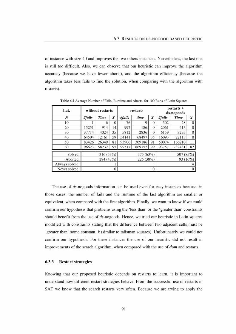
6.3 RESULTS ON DS-NOGOOD BASED HEURISTIC
91
of instance with size 40 and improves the two others instances. Nevertheless, the last one
is still too difficult. Also, we can observe that our heuristic can improve the algorithm
accuracy (because we have fewer aborts), and the algorithm efficiency (because the
algorithm takes less fails to find the solution, when comparing with the algorithm with
restarts).
Table 6.2 Average Number of Fails, Runtime and Aborts, for 100 Runs of Latin Squares
Lat. without restarts restarts restarts +
ds-nogoods
N #fails Time X #fails time X #fails Time X
10 1 6 0 76 9 0 502 28 0 20 15251 914 14 997 186 0 2061 413 0 30 37714 4024 35 5812 2836 0 6159 3295 0 40 64504 12161 59 54141 68497 35 16093 22113 0 50 83426 26349 81 93906 309186 91 50074 166210 11 60 96623 58232 95 99517 869752 99 93757 732481 82 Solved: 316 (53%) 375 (63%) 507 (85%)
Aborted: 284 (47%) 225 (38%) 93 (16%) Always solved: 1 3 4
Never solved: 0 0 0
The use of ds-nogoods information can be used even for easy instances because, in
those cases, the number of fails and the runtime of the last algorithm are smaller or
equivalent, when compared with the first algorithm. Finally, we want to know if we could
confirm our hypothesis that problems using the ‘less than’ or the ‘greater than’ constraints
should benefit from the use of ds-nogoods. Hence, we tried our heuristic in Latin squares
modified with constraints stating that the difference between two adjacent cells must be
‘greater than’ some constant, k (similar to talisman squares). Unfortunately we could not
confirm our hypothesis. For these instances the use of our heuristic did not result in
improvements of the search algorithm, when compared with the use of dom and restarts.
6.3.3 Restart strategies
Knowing that our proposed heuristic depends on restarts to learn, it is important to
understand how different restart strategies behave. From the successful use of restarts in
SAT we know that the search restarts very often. Because we are trying to apply the

6 USING DS-NOGOODS IN HEURISTICS
92
successful ideas of SAT (namely, restarts), we think that for CP(FD) algorithms to benefit
from restarts, the search algorithm should be allowed to restart a sufficient number of
times. What we mean is that, if restarts really matter, which is our case, then frequent
restarts should be more useful.
So, in this section, we compare different restart strategies for the harder instances,
where we already have seen that restarts play an important role. Because we know that
restarts are needed for solving these instances, we are trying to understand the impact of
different restart strategies.
Table 6.3 Comparing Different Restart Strategies
strategy (8;1) (9;1) (10;1)
#fails time X #fails Time X #fails time X
+1 (95) 35144 4059 7 53941 7066 26 80319 14218 63 +5 (82) 39482 4518 9 44614 5752 14 80283 11412 60
+10 (73) 40192 5485 15 44104 7008 15 82386 15029 66 +20 (62) 33995 4698 6 51050 8040 24 76950 14065 56 +50 (46) 37236 5117 11 51569 8012 25 80040 14337 63
+100 (36) 50209 6974 19 48784 7418 26 79455 13797 64 *1.01 (69) 39349 4606 9 50275 6406 22 80625 11392 59 *1.05 (36) 41443 5559 13 51927 7912 26 79059 12657 63 *1.1 (25) 47151 6018 19 62378 9466 39 88565 14848 72 *1.5 (9) 57805 7477 41 70436 10103 52 93896 15302 87 *2 (6) 75173 9611 62 81465 11512 69 94013 15659 90
Luby (44) 46217 5092 17 62419 7663 36 77481 10467 60
Table 6.3 compares different restart strategies for the harder instances of talisman
squares. We use the third algorithm, which uses restarts and our ds-nogood heuristic,
dom+act. Recall that we use ds-nogoods only to compute the heuristic and we do not post
nogoods as constraints in the solver. The first lines of the table, identified by a plus signal
(+) and a value, represent a linear incremental strategy on the cutoff (defined to be the
number of fails) by the value specified. The next group of lines, identified by a star signal
(*) and a value, represent a geometrical incremental restart strategy (Walsh, 1999) on the
cutoff by the value specified. The last strategy, in the last line, uses the Luby sequence
(Luby et al., 1993). The number in parentheses indicates the number of restarts needed to
reach the predefined limit of 100000 fails, knowing that the initial cutoff value is always
1000 fails.

6.4 REFINING THE SEARCH ALGORITHM
93
For each instance we run each strategy 100 times and Table 6.3 presents the average
number of fails, the average runtime in milliseconds and the number of aborts (X).
The results shown are not conclusive about the best linear strategy. But, in the
geometrical strategies we can conclude that a high geometrical factor (fast growing of the
cutoff value) has a poor behavior when compared to lower geometrical factors. We can
also observe that the geometrical strategy only has a performance compared with the
linear strategy when the geometrical factor is very low and the number of restarts starts to
be near the ones of the incremental strategy. Even the Luby strategy, that is known to be
in a log factor of the optimal, has a poor behavior.
Note that restarts are not independent from each other, since information from past
restarts is used in the following restarts, in the variable selection heuristic. In our case,
restarting means learning information from ds-nogoods into the dom+act heuristic, and
so, the algorithm needs to restart, at least, a minimum number of times to learn. Hence,
we can conclude that, for these instances, frequent restarts are better. We can also observe
that the geometrical strategy is as good as the incremental one only when the geometrical
factor is very low, and so, in this sense, we can say that a linear incremental restart
strategy is better than a geometrical one, in our case.
Also, because of the need of learning we need to restart often, and because the
different incremental restarts strategies do not seem to be very different, for the ongoing
empirical evaluation we opt by maintaining an incremental restart strategy with an
increment of 5 fails. Of course, this could be problem dependent, and, even for the same
problem, it could be dependent on the instance size. Even so, using always the same
configuration for the restart strategy allows us to compare results.
6.4 REFINING THE SEARCH ALGORITHM
Results presented in the previous sections allow us to conclude that information within
ds-nogoods is of some use for the variable selection heuristic, which resulted in the
improvement of the search algorithm for some instances. Despite the improvements, they
were not very strong, nor could we confirm these results for other instances. So, after we
6 USING DS-NOGOODS IN HEURISTICS
94
have shown that our ds-nogood based heuristic could be used with success in some
instances, we tried to fine tune the algorithm that uses our dom+act heuristic. We started
by testing different forms of choosing the branching value, i.e., the value selection
heuristic. Recall that, in the already presented empirical results, we have used a randomly
selected value. And then, we have generalized the order of the branches out of each
decision node, which turned out to be very important for the success of the search
algorithm.
In domain splitting search we want to split the domain, so the lexicographic order is
not considered. If not, in practice, the search algorithm will fall in a 2-way branching
scheme. It selects the first value in the left branch and the right branch corresponds to the
refutation. As an example, consider a variable x with domain dx={v1, …, vk}. Then, if we
choose the values in lexicographic order the left branch will be x ≤ v1 and the right branch
will be x>v1. In practice this is equivalent to a 2-way like branching decision, the decision
of x = v1 and the refutation, x≠v1, respectively.
But because our strategy selects the value randomly, the previous situation could
occur and, possibly, disturb the domain splitting search. So, instead of selecting the value
randomly we have tried to select the value in the middle of the domain. In this way the
domain is split in two equally sized sets. This allows us to have a balanced search tree,
which reduces the highest depth of the search tree. Consider, as an example, that we have
a problem with n variables and that all variables have the same domain size d. If, for one
variable we choose for branching the middle value, and then continue selecting that
variable until the variable becomes assigned, the height of this binary tree is O(log2d).
Because we have n variables the height of the search tree is O(n.log2d). On the other side,
if we choose for branching the right most value of the domain, the left branch needs O(d)
decisions until the variable is assigned a value. And because we have n variables the
maximum height of the search tree is O(n.d). Intuitively, we should avoid deeper
branches, because the search effort will be bigger, and so, minimizing the height of the
search tree, i.e., choosing the middle value for branching, should be better. Notice that, as
explained in the original paper, the fail first principle (Haralick and Elliott, 1979) tries to
minimize the branch depth. So, using a strategy that helps the FF principle should be
important.

6.4 REFINING THE SEARCH ALGORITHM
95
Thus, we have tested this middle value selection strategy, in the problem instances
that had good results for our dom+act heuristic, the Talisman square and the Latin
squares. We could not find improvements in the results that we had already obtained, nor
deterioration of those results. Roughly, the results were equivalent. We have no
theoretical explanation for this. But, because we have the constraint propagation
mechanism, even a branching decision that maintains a big domain size could effectively
prune the search space.
It could be relevant to branch first on smaller sets of the domain. This will create
smaller search trees in the left branches, and postpone for the right branches the bigger
sets, only if the solution is not found first. So, instead of dividing the domain in half we
have divided the domain in four. Then, the search branchs first on the left smaller set.
With this approach to domain splitting search we could not find better results, when
comparing with randomly selecting a value.
Our dom+act variable branching heuristic collects information from ds-nogoods with
success. So, we have also tried to collect information from ds-nogoods, but now for the
value selection heuristic. The intuition behind this heuristic is that we should try, for the
selected variable, the set of values that are more common for that variable in ds-nogoods
as a positive decision or as a negative decision. But, because in the domain splitting
branching we narrow domains this heuristic needs to analyse all the decisions in ds-
nogoods, related with the selected variable. So, this value decision uses two counters,
countPos and countNeg, initialized to zero. These counters count the occurrence of the
variable in ds-nogoods as a positive decision or as a negative decision, respectively.
Associated with these counters we collect, respectively, the maximum value that appears
in a positive decision, maxPos, and the minimum value that appears in a negative
decision, minNeg. These two values represent the value that includes more other values
appearing in the ds-nogoods, as a positive or as a negative decision, respectively. Then,
this value heuristic selects the value with the higher counter. If the two counters are equal
a value is selected between MIN(minNeg, maxPos) and MAX(minNeg, maxPos). If the
variable does not occur in ds-nogoods then this value heuristic falls in the rand value
heuristic. Note that this heuristic tries to identify where the biggest cluster of values
appearing in ds-nogoods is, and splits the domain such that the bigger clusters are not
6 USING DS-NOGOODS IN HEURISTICS
96
broken. This means staying in one of the sides of the domain splitting. Unfortunately, and
again, we could not see improvement results when using this ds-nogood based value
heuristic, considering the results already obtained for the Talisman and Latin squares.
So, because we do not see advantages on using none of the explained strategies for
the value selection heuristic, and for the sake of flexibility we opt by maintaining a
random selection of values from the actual domain of variables. Though this could not be
the best strategy, because of the non-deterministic nature, it has the advantages of
minimizing possible recurrent bad decisions.
6.4.1 Flexible Domain-splitting branching
We propose to generalize the order of the left and right branch of the domain splitting
search. As already explained, the decision in the left branch is done first and is called a
positive decision. It corresponds to constraining the variable to the left part of the domain,
e.g. x ≤ 5. The decision on the right branch is called a negative decision, and corresponds
to the refutation of the left branch, i.e., it constrains the variable to the right part of the
domain, e.g. x>5. The negative decision represents the negation of the positive decision.
Thus, due to the intrinsic operation of domain splitting search, a negative decision is
only done when a positive decision fails. This means that the search first tries the positive
decisions for the variables. And because the first decisions are typically narrowing the
domains of variables, in the beginning of the search tree we will have many positive
decisions reducing the domains to the left part. But there is no reason for trying first the
left part of the domains of variable. Suppose, for instance, that the solution for a problem
is in the right part of the domains of some of the variables. Then, the search will be lost
trying the values of the left part, until everything fails. Only then the search could try the
right part of the domains. So, the branching should be more flexible in choosing the part
of the domain to try first.
The positive and negative decisions are a formalism. They are what they are only by
definition. This particular definition is favoring some parts of the search space. Therefore
we could say that the search is biased by the definition. So, we propose to generalize the
notion of positive decision, which could constrain the domain to the left or to the right
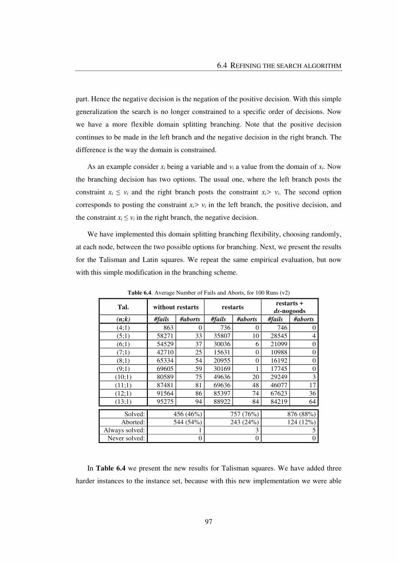
6.4 REFINING THE SEARCH ALGORITHM
97
part. Hence the negative decision is the negation of the positive decision. With this simple
generalization the search is no longer constrained to a specific order of decisions. Now
we have a more flexible domain splitting branching. Note that the positive decision
continues to be made in the left branch and the negative decision in the right branch. The
difference is the way the domain is constrained.
As an example consider xi being a variable and vi a value from the domain of xi. Now
the branching decision has two options. The usual one, where the left branch posts the
constraint xi ≤ vi and the right branch posts the constraint xi> vi. The second option
corresponds to posting the constraint xi> vi in the left branch, the positive decision, and
the constraint xi ≤ vi in the right branch, the negative decision.
We have implemented this domain splitting branching flexibility, choosing randomly,
at each node, between the two possible options for branching. Next, we present the results
for the Talisman and Latin squares. We repeat the same empirical evaluation, but now
with this simple modification in the branching scheme.
Table 6.4. Average Number of Fails and Aborts, for 100 Runs (v2)
Tal. without restarts restarts restarts +
ds-nogoods
(n;k) #fails #aborts #fails #aborts #fails #aborts
(4;1) 863 0 736 0 746 0 (5;1) 58271 33 35807 10 28545 4 (6;1) 54529 37 30036 6 21099 0 (7;1) 42710 25 15631 0 10988 0 (8;1) 65334 54 20955 0 16192 0 (9;1) 69605 59 30169 1 17745 0
(10;1) 80589 75 49636 20 29249 3 (11;1) 87481 81 69636 48 46077 17 (12;1) 91564 86 85397 74 67623 36 (13;1) 95275 94 88922 84 84219 64
Solved: 456 (46%) 757 (76%) 876 (88%)
Aborted: 544 (54%) 243 (24%) 124 (12%) Always solved: 1 3 5
Never solved: 0 0 0
In Table 6.4 we present the new results for Talisman squares. We have added three
harder instances to the instance set, because with this new implementation we were able
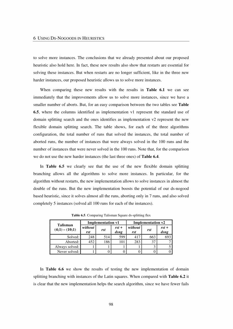
6 USING DS-NOGOODS IN HEURISTICS
98
to solve more instances. The conclusions that we already presented about our proposed
heuristic also hold here. In fact, these new results also show that restarts are essential for
solving these instances. But when restarts are no longer sufficient, like in the three new
harder instances, our proposed heuristic allows us to solve more instances.
When comparing these new results with the results in Table 6.1 we can see
immediately that the improvements allow us to solve more instances, since we have a
smaller number of aborts. But, for an easy comparison between the two tables see Table
6.5, where the columns identified as implementation v1 represent the standard use of
domain splitting search and the ones identifies as implementation v2 represent the new
flexible domain splitting search. The table shows, for each of the three algorithms
configuration, the total number of runs that solved the instances, the total number of
aborted runs, the number of instances that were always solved in the 100 runs and the
number of instances that were never solved in the 100 runs. Note that, for the comparison
we do not use the new harder instances (the last three ones) of Table 6.4.
In Table 6.5 we clearly see that the use of the new flexible domain splitting
branching allows all the algorithms to solve more instances. In particular, for the
algorithm without restarts, the new implementation allows to solve instances in almost the
double of the runs. But the new implementation boosts the potential of our ds-nogood
based heuristic, since it solves almost all the runs, aborting only in 7 runs, and also solved
completely 5 instances (solved all 100 runs for each of the instances).
Table 6.5. Comparing Talisman Square ds-splitting flex
Talisman
(4;1) – (10;1)
Implementation v1 Implementation v2
without
rst rst
rst +
dsng
without
rst rst
rst +
dsng
Solved: 248 514 599 417 663 693 Aborted: 452 186 101 283 37 7
Always solved: 1 1 1 1 3 5 Never solved: 1 0 0 0 0 0
In Table 6.6 we show the results of testing the new implementation of domain
splitting branching with instances of the Latin squares. When compared with Table 6.2 it
is clear that the new implementation helps the search algorithm, since we have fewer fails

6.4 REFINING THE SEARCH ALGORITHM
99
and aborts. Nevertheless, when using our ds-nogoods based heuristic with the new
implementation, the results are better, but not so significant.
Table 6.6. Average Number of Fails and Aborts, for 100 Runs of Latin Squares (v2)
Lat. without restarts restarts restarts +
ds-nogoods
N #fails #aborts #fails #aborts #fails #aborts
10 1 0 0 0 0 0 20 15251 14 155 0 229 0 30 37714 35 1368 0 1222 0 40 64504 59 4287 0 3642 0 50 83426 81 30690 5 20066 2 60 96623 95 91759 84 73511 55
Solved: 316 (53%) 511 (85%) 543 (91%)
Aborted: 284 (47%) 89 (15%) 57 (10%) Always solved: 1 4 4
Never solved: 0 0 0
We have tried to use harder instances of Talisman squares. Recall that a Talisman
squares (n,k) is a magic square of size n with additional constraints stating that the
difference between any two adjacent cells must be greater than some constant k. We have
tried various harder instances of different sizes of talisman square, where we use values
for k greater than 1. But, invariably, all the combinations revealed to be very hard for all
the three algorithms configuration tested.
We use Talisman squares because we have made an assumption that if the problem
has constraints related with mathematical inequalities, the use of domain splitting could
be adequate, since it also uses inequalities. So, we tried another version of the Talisman
square, for which the magic square related constraints were removed, which we call
Original Talisman square. We then define a set of instances, with different combinations
of (n,k), which are very hard for the dom heuristic, with and without restarts.

6 USING DS-NOGOODS IN HEURISTICS
100
Table 6.7. Average Number of Fails and Aborts, for 100 Runs of Talisman Squares (Original)
Tal-O without restarts restarts restarts + ds-
nogoods
(n;k) #fails #aborts #fails #aborts #fails #aborts
(5;4) 98003 96 99713 99 78723 53 (6;5) 99010 98 89500 77 32948 2 (7;6) 97225 95 85532 73 22129 0 (7;7) 99534 99 99918 100 84727 67 (8;8) 99064 99 95924 91 54428 16
(9;10) 100000 100 99682 99 74382 41 (10;9) 92954 91 38800 10 11654 0 (10;10) 99006 99 85377 69 27940 2 (10;11) 100000 100 96624 96 45737 9 (10;12) 100000 100 99918 100 85145 64 (11;10) 91307 90 34896 9 11401 0 (11;11) 96732 96 72154 56 21070 0 (11;12) 100000 100 94525 91 38379 7 (11;13) 100000 100 99433 99 62956 21
Solved: 37 (03%) 331 (24%) 1118 (80%) Aborted: 1363 (97%) 1069 (76%) 282 (20%)
Always solved: 0 0 4 Never solved: 5 2 0
In Table 6.7 we present the results of running the three algorithms configuration on
instances of the Original Talisman square. As it can be seen, those instances are very hard
when using only backtrack search without restarts. In fact, from the 1400 total runs (14
instances and 100 runs for each instance), only 37 runs could find the solution, which
corresponds to only 3% of the total number of runs. And, for 5 instances all the runs have
aborted. But, when using restarts the number of solved instances grows by an order of
magnitude. Still, in this case the number aborted runs is high, since 76% of the runs
aborted. And we have 2 instances for which all the runs have aborted.
For the instances in Table 6.7 the use of our ds-nogood heuristic is crucial, since it
allows to solve 80% of the runs. This corresponds to an increment of 56 percentage points
when compared to the algorithm that uses only restarts, and an increment of 77
percentage point when compared to the algorithm without restarts. Also note that 4
instances were solved in all the runs and none of the instances were unsolved (instances
for which the algorithm always aborts). Those results support the relevance of our
proposed heuristic, which proved to be more than a simple tie break for the dom heuristic,
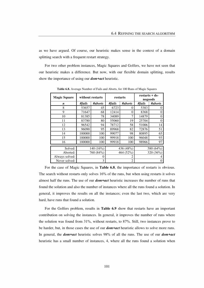
6.4 REFINING THE SEARCH ALGORITHM
101
as we have argued. Of course, our heuristic makes sense in the context of a domain
splitting search with a frequent restart strategy.
For two other problem instances, Magic Squares and Golfers, we have not seen that
our heuristic makes a difference. But now, with our flexible domain splitting, results
show the importance of using our dom+act heuristic.
Table 6.8. Average Number of Fails and Aborts, for 100 Runs of Magic Squares
Magic Square without restarts restarts restarts + ds-
nogoods
n #fails #aborts #fails #aborts #fails #aborts
8 53657 45 6723 0 5383 0 9 71647 68 12414 0 8368 0 10 81385 78 34089 7 14879 0 11 83780 80 55060 19 25704 0 12 96542 94 78712 58 51006 14 13 96090 95 89968 82 72876 51 14 100000 100 99077 98 80895 65 15 100000 100 99918 100 96048 93 16 100000 100 99918 100 98966 97
Solved: 140 (16%) 436 (48%) 580 (64%) Aborted: 760 (84%) 464 (52%) 320 (36%)
Always solved: 0 2 4 Never solved: 3 2 0
For the case of Magic Squares, in Table 6.8, the importance of restarts is obvious.
The search without restarts only solves 16% of the runs, but when using restarts it solves
almost half the runs. The use of our dom+act heuristic increases the number of runs that
found the solution and also the number of instances where all the runs found a solution. In
general, it improves the results on all the instances; even the last two, which are very
hard, have runs that found a solution.
For the Golfers problem, results in Table 6.9 show that restarts have an important
contribution on solving the instances. In general, it improves the number of runs where
the solution was found from 31%, without restarts, to 87%. Still, two instances prove to
be harder, but, in those cases the use of our dom+act heuristic allows to solve more runs.
In general, the dom+act heuristic solves 98% of all the runs. The use of our dom+act
heuristic has a small number of instances, 4, where all the runs found a solution when

6 USING DS-NOGOODS IN HEURISTICS
102
compared to the use of restarts, 6. But, if we look closer, we have instances where only
one run aborted and the number of fails is smaller.
Table 6.9. Average Number of Fails and Aborts, for 100 Runs of Golfers v2
Golfers without restarts restarts restarts +
ds-nogoods
(g;s;w) #fails #aborts #fails #aborts #fails #aborts
(6,3,6) 52297 39 19498 0 12588 1 (6,3,7) 59829 30 88861 81 54956 17 (7,5,2) 88213 88 10436 0 9161 1 (8,5,2) 90120 90 12410 0 9859 0 (6,4,3) 76044 74 10792 0 12186 1 (7,4,3) 94887 94 20614 3 17863 0 (5,4,4) 44467 37 8480 0 9964 0 (7,3,4) 88814 87 27270 3 16445 2 (6,3,5) 64522 55 11433 0 11141 0 (8,3,5) 97133 95 67824 47 26760 3
Solved: 311 (31%) 866 (87%) 975 (98%)
Aborted: 689 (69%) 134 (13%) 25 (2%) Always solved: 0 6 4
Never solved: 0 0 0
We think that a clear conclusion can be taken from this section. Indeed, we can
confirm the first results that unveil the possible use of information within ds-nogoods.
The simple enhancement made in the branching scheme, a more flexible domain splitting,
improves the search algorithm, allowing to solve more runs, more instances and failing
less.
6.4.2 Importance of domain-splitting branching
It is important to understand whether the good results of our dom+act heuristic, presented
so far, are somehow related with the branching used. As we already explained our work is
inspired by the successful use of restarts in SAT solvers, and also by the use of nogoods
from restarts in the context of 2-way branching in CP(FD). So, we are interested in
investigating whether our proposed heuristic is also useful in 2-way branching. We want
to see if branching has impact in the algorithms, namely, we are interested in verifying if
domain splitting is better than 2-way branching. Since we have argue that domain
splitting branching is similar to the branching employed in SAT, it should be expected
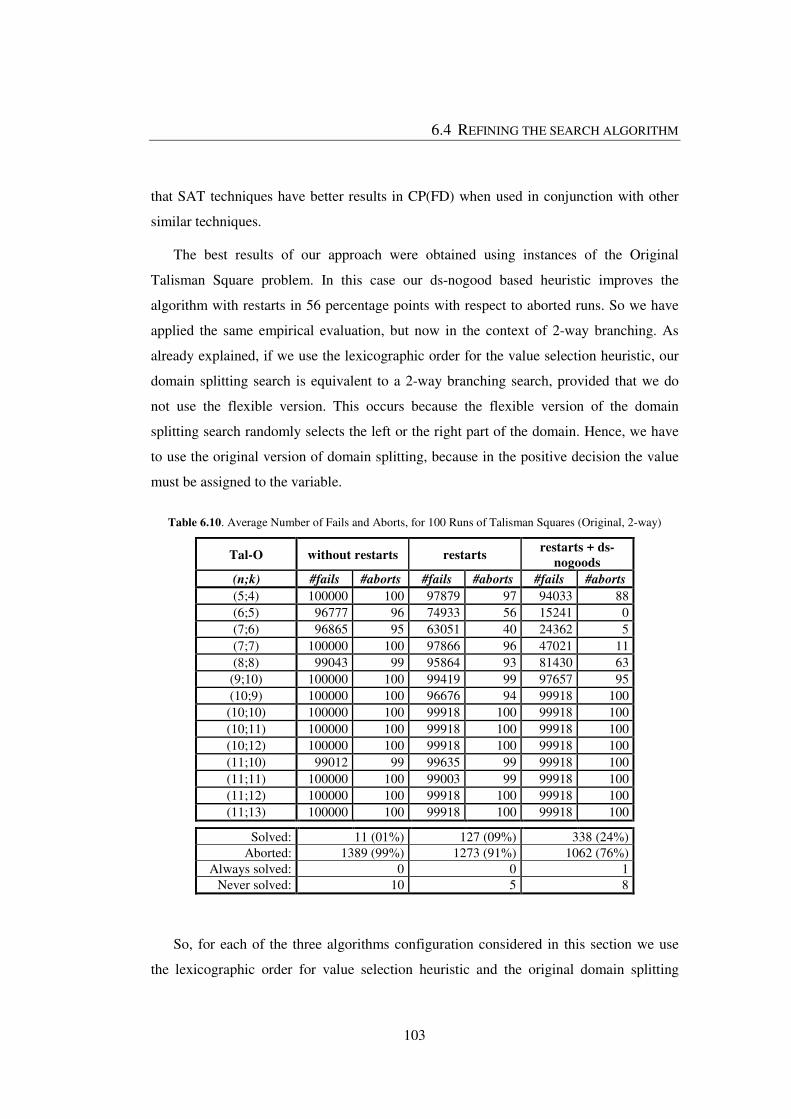
6.4 REFINING THE SEARCH ALGORITHM
103
that SAT techniques have better results in CP(FD) when used in conjunction with other
similar techniques.
The best results of our approach were obtained using instances of the Original
Talisman Square problem. In this case our ds-nogood based heuristic improves the
algorithm with restarts in 56 percentage points with respect to aborted runs. So we have
applied the same empirical evaluation, but now in the context of 2-way branching. As
already explained, if we use the lexicographic order for the value selection heuristic, our
domain splitting search is equivalent to a 2-way branching search, provided that we do
not use the flexible version. This occurs because the flexible version of the domain
splitting search randomly selects the left or the right part of the domain. Hence, we have
to use the original version of domain splitting, because in the positive decision the value
must be assigned to the variable.
Table 6.10. Average Number of Fails and Aborts, for 100 Runs of Talisman Squares (Original, 2-way)
Tal-O without restarts restarts restarts + ds-
nogoods
(n;k) #fails #aborts #fails #aborts #fails #aborts
(5;4) 100000 100 97879 97 94033 88 (6;5) 96777 96 74933 56 15241 0 (7;6) 96865 95 63051 40 24362 5 (7;7) 100000 100 97866 96 47021 11 (8;8) 99043 99 95864 93 81430 63
(9;10) 100000 100 99419 99 97657 95 (10;9) 100000 100 96676 94 99918 100 (10;10) 100000 100 99918 100 99918 100 (10;11) 100000 100 99918 100 99918 100 (10;12) 100000 100 99918 100 99918 100 (11;10) 99012 99 99635 99 99918 100 (11;11) 100000 100 99003 99 99918 100 (11;12) 100000 100 99918 100 99918 100 (11;13) 100000 100 99918 100 99918 100
Solved: 11 (01%) 127 (09%) 338 (24%) Aborted: 1389 (99%) 1273 (91%) 1062 (76%)
Always solved: 0 0 1 Never solved: 10 5 8
So, for each of the three algorithms configuration considered in this section we use
the lexicographic order for value selection heuristic and the original domain splitting

6 USING DS-NOGOODS IN HEURISTICS
104
branching, which in practice results in a 2-way branching. In Table 6.10 we have the
results of using a 2-way branching scheme without restarts, with restarts and with our
proposed heuristic. From the results, it is obvious that our approach does not work in the
context of 2-way branching. The use of restarts allows solving some more instances, but
still 91% of the runs have aborted. But, when using our ds-nogood heuristic we only see a
small impact, since it could only solve 24% of the runs, and for 8 instances it never found
a solution.
The results with 2-way branching are really very bad when compared with domain-
splitting branching. We do not have any justifications for this situation. In fact, the
difference is very high; nevertheless, our dom+act heuristic improves by 15% the
algorithm with restarts. This fact also supports the importance of our ds-nogoods based
heuristic. Which means that, even with other branching scheme, the heuristic is also
valuable, since it can collect useful information from ds-nogoods. Of course, it is better
with domain-splitting search, which somehow empower the dom+act heuristic.
These results are somehow expected, since our heuristic uses information from
domain splitting nogoods, which makes the heuristic more fitted for this context. On the
other hand these results could support our argumentation stating that domain splitting is
more similar to SAT than it is 2-way. As a consequence it is better for applying other
SAT related techniques, namely, clause recording (nogood recording), restarts, and
heuristics based on nogoods.
6.5 COMPARING WITH DOM/WDEG
Because we use nogoods extracted from restarts and because the successful use of the
dom/wdeg heuristic in the context of nogood recording from restarts (Lecoutre et al.,
2007b, 2007a), it is important that we try the dom/wdeg heuristic in our work. This is a
conflict driven heuristic that is considered state of the art. We apply and evaluate this
heuristic in the context of domain splitting search. This allows us to evaluate the
importance of this heuristic in our particular context and also to compare this heuristic
with our ds-nogoods based heuristic (dom+act).
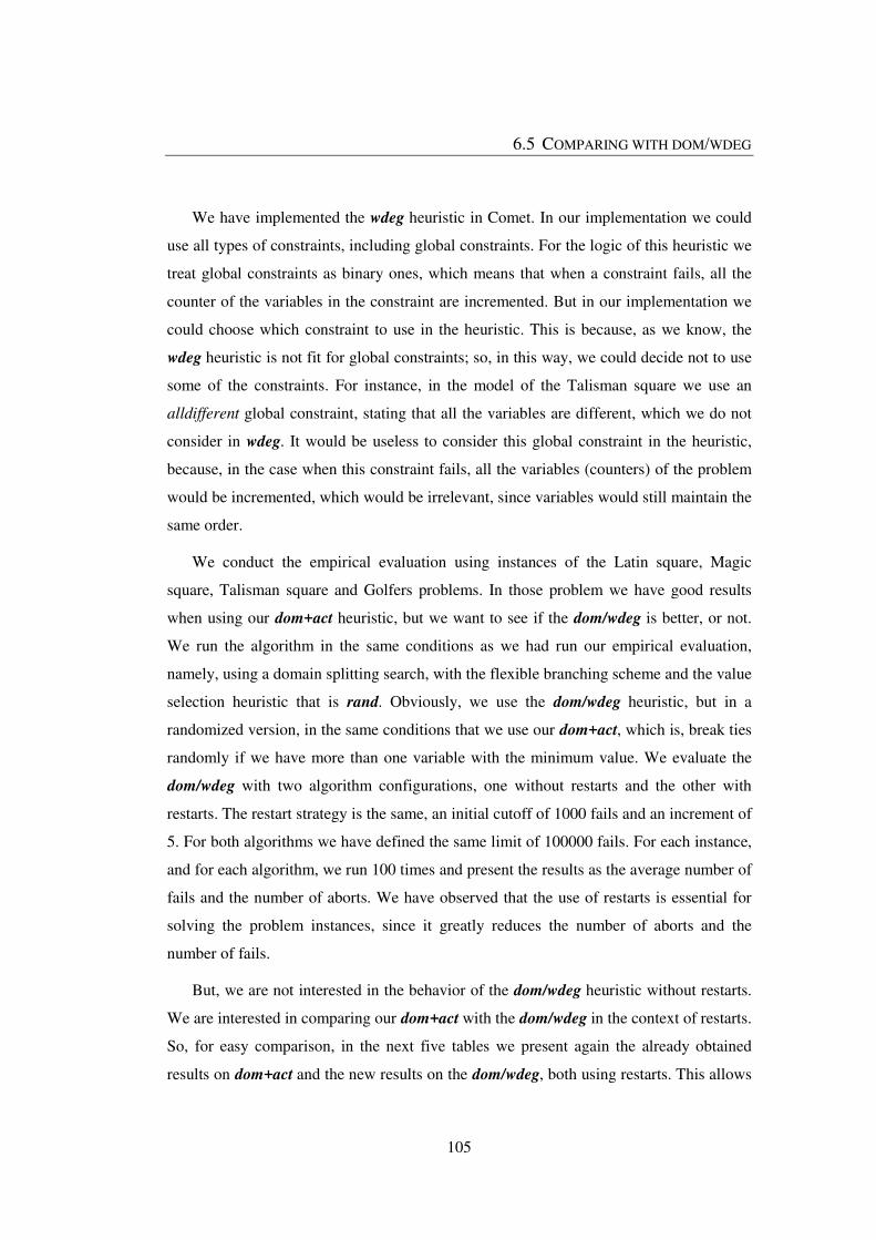
6.5 COMPARING WITH DOM/WDEG
105
We have implemented the wdeg heuristic in Comet. In our implementation we could
use all types of constraints, including global constraints. For the logic of this heuristic we
treat global constraints as binary ones, which means that when a constraint fails, all the
counter of the variables in the constraint are incremented. But in our implementation we
could choose which constraint to use in the heuristic. This is because, as we know, the
wdeg heuristic is not fit for global constraints; so, in this way, we could decide not to use
some of the constraints. For instance, in the model of the Talisman square we use an
alldifferent global constraint, stating that all the variables are different, which we do not
consider in wdeg. It would be useless to consider this global constraint in the heuristic,
because, in the case when this constraint fails, all the variables (counters) of the problem
would be incremented, which would be irrelevant, since variables would still maintain the
same order.
We conduct the empirical evaluation using instances of the Latin square, Magic
square, Talisman square and Golfers problems. In those problem we have good results
when using our dom+act heuristic, but we want to see if the dom/wdeg is better, or not.
We run the algorithm in the same conditions as we had run our empirical evaluation,
namely, using a domain splitting search, with the flexible branching scheme and the value
selection heuristic that is rand. Obviously, we use the dom/wdeg heuristic, but in a
randomized version, in the same conditions that we use our dom+act, which is, break ties
randomly if we have more than one variable with the minimum value. We evaluate the
dom/wdeg with two algorithm configurations, one without restarts and the other with
restarts. The restart strategy is the same, an initial cutoff of 1000 fails and an increment of
5. For both algorithms we have defined the same limit of 100000 fails. For each instance,
and for each algorithm, we run 100 times and present the results as the average number of
fails and the number of aborts. We have observed that the use of restarts is essential for
solving the problem instances, since it greatly reduces the number of aborts and the
number of fails.
But, we are not interested in the behavior of the dom/wdeg heuristic without restarts.
We are interested in comparing our dom+act with the dom/wdeg in the context of restarts.
So, for easy comparison, in the next five tables we present again the already obtained
results on dom+act and the new results on the dom/wdeg, both using restarts. This allows
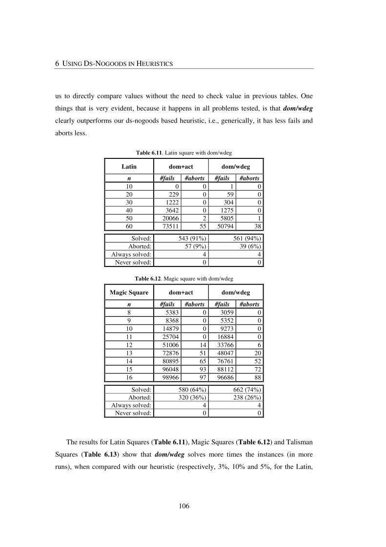
6 USING DS-NOGOODS IN HEURISTICS
106
us to directly compare values without the need to check value in previous tables. One
things that is very evident, because it happens in all problems tested, is that dom/wdeg
clearly outperforms our ds-nogoods based heuristic, i.e., generically, it has less fails and
aborts less.
Table 6.11. Latin square with dom/wdeg
Latin dom+act dom/wdeg
n #fails #aborts #fails #aborts
10 0 0 1 0 20 229 0 59 0 30 1222 0 304 0 40 3642 0 1275 0 50 20066 2 5805 1 60 73511 55 50794 38
Solved: 543 (91%) 561 (94%)
Aborted: 57 (9%) 39 (6%) Always solved: 4 4
Never solved: 0 0
Table 6.12. Magic square with dom/wdeg
Magic Square dom+act dom/wdeg
n #fails #aborts #fails #aborts
8 5383 0 3059 0 9 8368 0 5352 0 10 14879 0 9273 0 11 25704 0 16884 0 12 51006 14 33766 6 13 72876 51 48047 20 14 80895 65 76761 52 15 96048 93 88112 72 16 98966 97 96686 88
Solved: 580 (64%) 662 (74%) Aborted: 320 (36%) 238 (26%)
Always solved: 4 4 Never solved: 0 0
The results for Latin Squares (Table 6.11), Magic Squares (Table 6.12) and Talisman
Squares (Table 6.13) show that dom/wdeg solves more times the instances (in more
runs), when compared with our heuristic (respectively, 3%, 10% and 5%, for the Latin,

6.5 COMPARING WITH DOM/WDEG
107
Magic and Talisman Squares). Nevertheless, the number of instances that were always
solved in the 100 runs is the same for the two heuristics. But, dom/wdeg always requires a
smaller number of fails in all instances of those problems, which indicate that it is more
efficient than dom+act.
We can say that, for those problem instances, the results of the two heuristics are
somehow aligned, because we observe roughly the same behavior of the search
algorithms. The easy instances are easily solved by the two heuristics. But, when the
instances start to be harder, both algorithms also start to have difficulties solving the
instances, needing more fails and aborting more runs.
Table 6.13. Talisman square with dom/wdeg
Talisman dom+act dom/wdeg
(n;k) #fails #aborts #fails #aborts
(4;1) 746 0 587 0 (5;1) 28545 4 19712 1 (6;1) 21099 0 11780 0 (7;1) 10988 0 7162 0 (8;1) 16192 0 9367 0 (9;1) 17745 0 12813 0
(10;1) 29249 3 22626 1 (11;1) 46077 17 32549 4 (12;1) 67623 36 51690 16 (13;1) 84219 64 75278 47
Solved: 876 (88%) 931 (93%)
Aborted: 124 (12%) 69 (7%) Always solved: 5 5
Never solved: 0 0
For instances of the Original Talisman Square problem, the utilization of the
dom/wdeg heuristic allows to solve more instances and with fewer fails, as can be
observed in Table 6.14. With the dom+act heuristic the search was able to solve 80% of
all the runs, but, when using the dom/wdeg that value grows to 98%. The dom/wdeg
heuristic has a better behavior on these instances, since it always uses fewer fails and
aborts less. Also, a large majority of instances were solved in all 100 runs, i.e., 11 out of
14. And 2 of the ones that were not solved in all runs, have a small number of aborts, 2
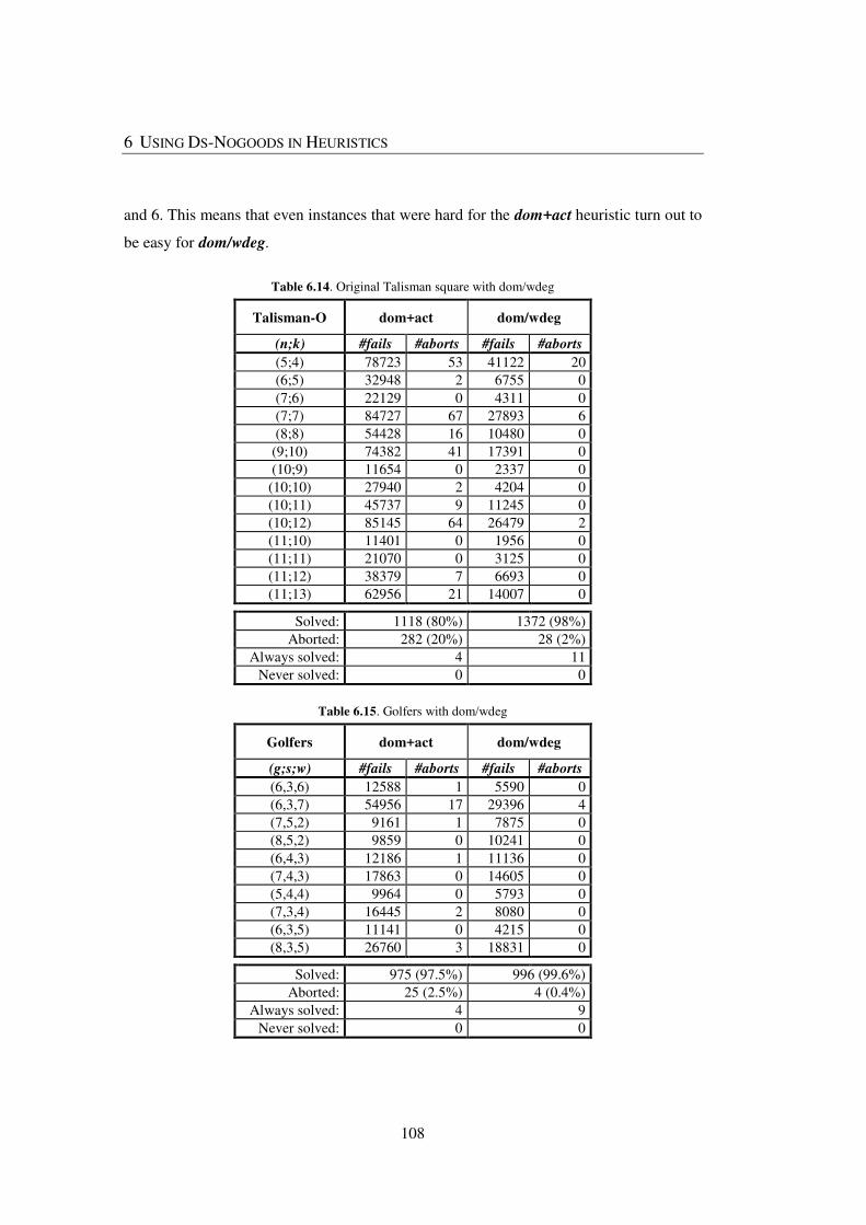
6 USING DS-NOGOODS IN HEURISTICS
108
and 6. This means that even instances that were hard for the dom+act heuristic turn out to
be easy for dom/wdeg.
Table 6.14. Original Talisman square with dom/wdeg
Talisman-O dom+act dom/wdeg
(n;k) #fails #aborts #fails #aborts
(5;4) 78723 53 41122 20 (6;5) 32948 2 6755 0 (7;6) 22129 0 4311 0 (7;7) 84727 67 27893 6 (8;8) 54428 16 10480 0
(9;10) 74382 41 17391 0 (10;9) 11654 0 2337 0 (10;10) 27940 2 4204 0 (10;11) 45737 9 11245 0 (10;12) 85145 64 26479 2 (11;10) 11401 0 1956 0 (11;11) 21070 0 3125 0 (11;12) 38379 7 6693 0 (11;13) 62956 21 14007 0
Solved: 1118 (80%) 1372 (98%)
Aborted: 282 (20%) 28 (2%) Always solved: 4 11
Never solved: 0 0
Table 6.15. Golfers with dom/wdeg
Golfers dom+act dom/wdeg
(g;s;w) #fails #aborts #fails #aborts
(6,3,6) 12588 1 5590 0 (6,3,7) 54956 17 29396 4 (7,5,2) 9161 1 7875 0 (8,5,2) 9859 0 10241 0 (6,4,3) 12186 1 11136 0 (7,4,3) 17863 0 14605 0 (5,4,4) 9964 0 5793 0 (7,3,4) 16445 2 8080 0 (6,3,5) 11141 0 4215 0 (8,3,5) 26760 3 18831 0
Solved: 975 (97.5%) 996 (99.6%)
Aborted: 25 (2.5%) 4 (0.4%) Always solved: 4 9
Never solved: 0 0
6.5 COMPARING WITH DOM/WDEG
109
For instances of the Golfers problem, results in Table 6.15 show that the dom/wdeg
heuristic allows the search algorithm to solve all instances in almost all the runs (only 4
runs aborted for one of the instances) and with fewer fails. For the dom+act heuristic the
number of aborts was higher when compared with dom/wdeg, even though it corresponds
to only 2.5% of all the runs.
Unfortunately, the results in this section mean that our proposed heuristic could not
outperform the state of the art dom/wdeg. Nevertheless, we can say that our heuristic is
right behind, since results are aligned and close to the ones of dom/wdeg. Despite that,
our heuristic incorporates useful information that could be of some use, namely, as we
will see later, it can indeed improve dom/wdeg.
6.5.1 Importance of domain splitting branching with dom/wdeg
We have observed that using our dom+act heuristic in the context of 2-way branching,
instead of domain splitting branching, results in a poor behavior of the search algorithm.
So, we want to investigate if the same behavior occurs with the dom/wdeg heuristic.
Hence, we have repeated the same empirical evaluation using 2-way splitting search
with instances of the Original Talisman Square (Table 6.10), but now using dom/wdeg
heuristic, with and without restarts. Surprisingly, with restarts, the search algorithm has
good results, almost as good as the use of domain splitting. Recall that with our dom+act
heuristic the search with 2-way splitting behaves very poorly. This situation could be
justified because our heuristic is developed in the context of domain splitting, more
specifically using information from ds-nogoods. This makes the heuristic unfitted for
other branching context. On the other hand, dom/wdeg, is unrelated with ds-nogoods, so it
would be more neutral when changing the branching strategies.
We have repeated the empirical evaluation of 2-way branching for instances of the
Latin and Talisman Squares, where there are harder instances for the dom/wdeg heuristic.
In Table 6.16 those results are presented and, for easy comparison, results on domain
splitting are also included. In parentheses, we have the number of instances included in
each of the problems considered, and in column #runs the total number of runs. The
column #fails is the sum of the average number of fails (‘k’ representing thousands). The
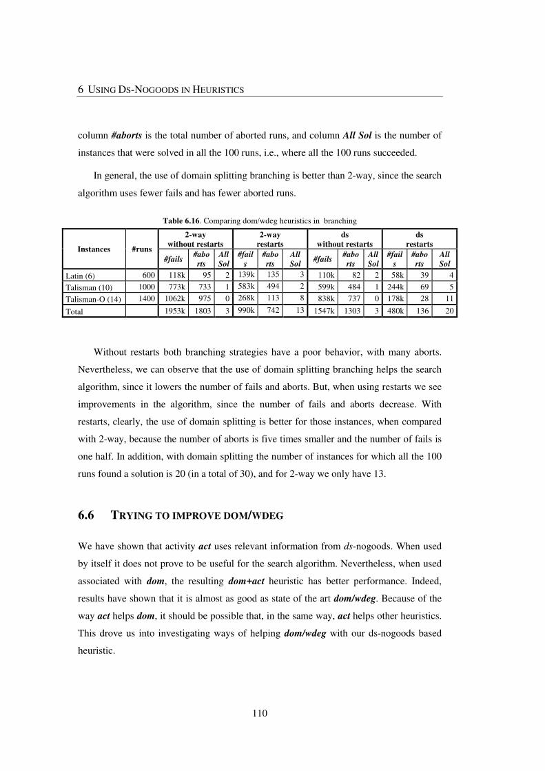
6 USING DS-NOGOODS IN HEURISTICS
110
column #aborts is the total number of aborted runs, and column All Sol is the number of
instances that were solved in all the 100 runs, i.e., where all the 100 runs succeeded.
In general, the use of domain splitting branching is better than 2-way, since the search
algorithm uses fewer fails and has fewer aborted runs.
Table 6.16. Comparing dom/wdeg heuristics in branching
Instances #runs
2-way
without restarts
2-way
restarts
ds
without restarts
ds
restarts
#fails #abo
rts
All
Sol
#fail
s
#abo
rts
All
Sol #fails
#abo
rts
All
Sol
#fail
s
#abo
rts
All
Sol
Latin (6) 600 118k 95 2 139k 135 3 110k 82 2 58k 39 4
Talisman (10) 1000 773k 733 1 583k 494 2 599k 484 1 244k 69 5
Talisman-O (14) 1400 1062k 975 0 268k 113 8 838k 737 0 178k 28 11
Total 1953k 1803 3 990k 742 13 1547k 1303 3 480k 136 20
Without restarts both branching strategies have a poor behavior, with many aborts.
Nevertheless, we can observe that the use of domain splitting branching helps the search
algorithm, since it lowers the number of fails and aborts. But, when using restarts we see
improvements in the algorithm, since the number of fails and aborts decrease. With
restarts, clearly, the use of domain splitting is better for those instances, when compared
with 2-way, because the number of aborts is five times smaller and the number of fails is
one half. In addition, with domain splitting the number of instances for which all the 100
runs found a solution is 20 (in a total of 30), and for 2-way we only have 13.
6.6 TRYING TO IMPROVE DOM/WDEG
We have shown that activity act uses relevant information from ds-nogoods. When used
by itself it does not prove to be useful for the search algorithm. Nevertheless, when used
associated with dom, the resulting dom+act heuristic has better performance. Indeed,
results have shown that it is almost as good as state of the art dom/wdeg. Because of the
way act helps dom, it should be possible that, in the same way, act helps other heuristics.
This drove us into investigating ways of helping dom/wdeg with our ds-nogoods based
heuristic.
6.6 TRYING TO IMPROVE DOM/WDEG
111
We have tried different combinations for incorporating the activity (act) of variables,
occurring in ds-nogoods, in the dom/wdeg heuristic. Some combinations have proved to
be worst, somehow deteriorating the dom/wdeg, with more aborts and fails. After some
dead ends we came up with a profitable combination that shows some interesting results.
The combination that shows promising results uses the act to fine tune the wdeg
component. We call this heuristic dom/wdeg+act and it is defined by choosing the
variable that satisfies the following expression.
min��..� % ���&'(�) *
+,-�.*/ (41)
The wdeg heuristic is also an activity based heuristic, but it only uses the activity of
variables in constraints that have failed. Therefore, by adding information of activity of
variables in ds-nogoods, the resulting heuristic is a more informed one. This new
heuristic, like the dom/wdeg, is also a ratio between the FF dom heuristic and the amount
of variables’ participation in failure (activity). But now, the activity also uses information
from occurrences of variables in ds-nogoods. In this sense we can say that the heuristic is
more accurate.
In Table 6.17 we compare our previous proposed dom+act heuristic with dom/wdeg
and with our novel heuristic dom/wdeg+act. The table shows the final results for each of
the problem instances that we use. In this way, it is easy to see, by means of our proposed
heuristics, the contribution of information within ds-nogoods, recorded from restarts. In
parentheses, we have the number of instances included in each of the problems
considered, and in column #runs the total number of runs. The column #fails is the sum
of the average number of fails (again, ‘k’ representing thousands). The column #aborts is
the total number of aborted runs, and column All Sol is the number of instances that were
solved in all the 100 runs, i.e., where all the 100 runs succeeded.
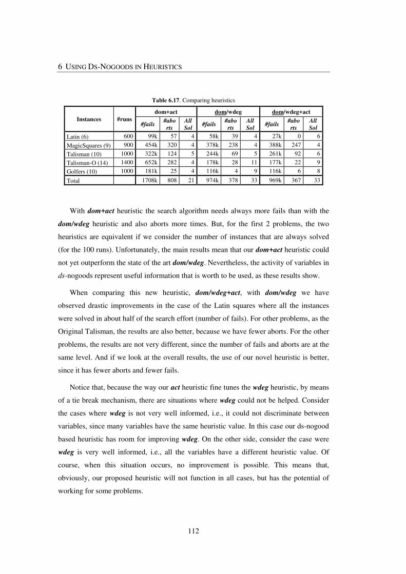
6 USING DS-NOGOODS IN HEURISTICS
112
Table 6.17. Comparing heuristics
Instances #runs
dom+act dom/wdeg dom/wdeg+act
#fails #abo
rts
All
Sol #fails
#abo
rts
All
Sol #fails
#abo
rts
All
Sol
Latin (6) 600 99k 57 4 58k 39 4 27k 0 6
MagicSquares (9) 900 454k 320 4 378k 238 4 388k 247 4
Talisman (10) 1000 322k 124 5 244k 69 5 261k 92 6
Talisman-O (14) 1400 652k 282 4 178k 28 11 177k 22 9
Golfers (10) 1000 181k 25 4 116k 4 9 116k 6 8
Total 1708k 808 21 974k 378 33 969k 367 33
With dom+act heuristic the search algorithm needs always more fails than with the
dom/wdeg heuristic and also aborts more times. But, for the first 2 problems, the two
heuristics are equivalent if we consider the number of instances that are always solved
(for the 100 runs). Unfortunately, the main results mean that our dom+act heuristic could
not yet outperform the state of the art dom/wdeg. Nevertheless, the activity of variables in
ds-nogoods represent useful information that is worth to be used, as these results show.
When comparing this new heuristic, dom/wdeg+act, with dom/wdeg we have
observed drastic improvements in the case of the Latin squares where all the instances
were solved in about half of the search effort (number of fails). For other problems, as the
Original Talisman, the results are also better, because we have fewer aborts. For the other
problems, the results are not very different, since the number of fails and aborts are at the
same level. And if we look at the overall results, the use of our novel heuristic is better,
since it has fewer aborts and fewer fails.
Notice that, because the way our act heuristic fine tunes the wdeg heuristic, by means
of a tie break mechanism, there are situations where wdeg could not be helped. Consider
the cases where wdeg is not very well informed, i.e., it could not discriminate between
variables, since many variables have the same heuristic value. In this case our ds-nogood
based heuristic has room for improving wdeg. On the other side, consider the case were
wdeg is very well informed, i.e., all the variables have a different heuristic value. Of
course, when this situation occurs, no improvement is possible. This means that,
obviously, our proposed heuristic will not function in all cases, but has the potential of
working for some problems.
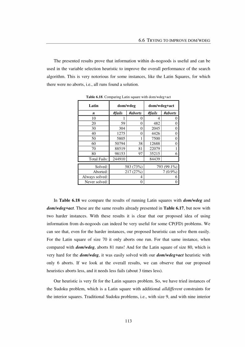
6.6 TRYING TO IMPROVE DOM/WDEG
113
The presented results prove that information within ds-nogoods is useful and can be
used in the variable selection heuristic to improve the overall performance of the search
algorithm. This is very notorious for some instances, like the Latin Squares, for which
there were no aborts, i.e., all runs found a solution.
Table 6.18. Comparing Latin square with dom/wdeg+act
Latin dom/wdeg dom/wdeg+act
n #fails #aborts #fails #aborts
10 1 0 4 0 20 59 0 482 0 30 304 0 2045 0 40 1275 0 4426 0 50 5805 1 7500 0 60 50794 38 12688 0 70 88519 81 22079 1 80 98153 97 35215 6
Total Fails: 244910 84439
Solved: 583 (73%) 793 (99.1%)
Aborted: 217 (27%) 7 (0.9%) Always solved: 4 6
Never solved: 0 0
In Table 6.18 we compare the results of running Latin squares with dom/wdeg and
dom/wdeg+act. These are the same results already presented in Table 6.17, but now with
two harder instances. With these results it is clear that our proposed idea of using
information from ds-nogoods can indeed be very useful for some CP(FD) problems. We
can see that, even for the harder instances, our proposed heuristic can solve them easily.
For the Latin square of size 70 it only aborts one run. For that same instance, when
compared with dom/wdeg, aborts 81 runs! And for the Latin square of size 80, which is
very hard for the dom/wdeg, it was easily solved with our dom/wdeg+act heuristic with
only 6 aborts. If we look at the overall results, we can observe that our proposed
heuristics aborts less, and it needs less fails (about 3 times less).
Our heuristic is very fit for the Latin squares problem. So, we have tried instances of
the Sudoku problem, which is a Latin square with additional alldifferent constraints for
the interior squares. Traditional Sudoku problems, i.e., with size 9, and with nine interior

6 USING DS-NOGOODS IN HEURISTICS
114
squares of 3 by 3, and pre-defined numbers are very easy. Indeed, we were able to solve,
even the ones that are considered very hard for humans, with small number of fails and
without restarts. Because our proposed approach needs restarts, it would not be useful for
those instances. Hence, we have tried Sudoku problems with bigger sizes.
Table 6.19. Testing Sudoku with dom/wdeg+act
Sudoku dom/wdeg dom/wdeg+act
n #fails #aborts #fails #aborts
25 504 0 714 0 36 45973 0 15938 0
Total Fails: 46477 16652
Table 6.19 summarizes the results we obtained with two instances of the Sudoku
problem. Those instances do not have pre-defined numbers, i.e., the Sudoku square is
empty. Instances of small size are very easy, typically solved without the need of restarts,
and instances of bigger size turn to be very hard, which we do not manage to solve. The
instance of size 25 is still easy; with both heuristics, the solution was found in all runs
with a small number of fails. For the other instance, again, both heuristics allow the
search to find a solution, for all the runs. But, our dom/wdeg+act heuristic needs almost 3
times less fails than dom/wdeg heuristic.
These results with Latin and Sudoku squares are not sole responsibility of the
heuristics. It is the interplay of restarts, nogood recording and heuristics based on
nogoods that allow us to improve the results of other heuristics.
6.7 SUMMARY AND FINAL REMARKS
In this chapter we have the main contributions of our work, related with using
information from ds-nogoods, extracted from restarts, in the variable selection heuristic.
This heuristic counts the activity of variables in nogoods and is used associated with the
fail first (FF) dom heuristic and dom/wdeg. The use of a heuristic based on nogoods
completes the proposed joint use of techniques, namely, restarts, nogoods and heuristics,
6.7 SUMMARY AND FINAL REMARKS
115
which were essential to improve SAT algorithms. We show that these techniques, when
used together, also help CP(FD) algorithms.
Our activity heuristic is not useful when used by itself. But, when associated with the
very important FF principle, it shows important improvements, when compared with the
FF dom heuristic. This allows us to conclude that, in fact, information within nogoods is
valuable and can be used to improve a CP(FD) algorithm. Indeed, we were able to
improve state-of-the-art dom/wdeg heuristic, which also uses the FF principle, when
associating our activity based heuristic. This allowed us to easily solve all the instances in
one of the problem classes and also to solve more difficult instances.
Our work and contribution are in the context of domain splitting search. We have also
tried to use the proposed heuristics in the context of the widely used 2-way branching
scheme. In this case, we have observed that our proposed heuristics also help the search,
but with less impact. And the overall results are below the ones with domain splitting
branching scheme. It seems that the use of domain splitting empowers our proposed
heuristics, which is what we expected, since the heuristics are using information from
domain splitting nogoods.

117
7 CONCLUSIONS AND FUTURE WORK
The utilization of restarts with nogoods recording in backtrack search algorithms for
solving CP(FD) problems is starting to be considered of great importance. This work is
inspired by the successful use of restarts in SAT and Lecoutre’s work on recording
nogoods from restarts in CP(FD), the so called nld-nogoods (Lecoutre et al., 2007a,
2007b). We generalized the nld-nogoods to the context of backtracking search algorithms
with domain-splitting and restarts. Additionally, we gave evidences that our proposed
nogoods have potentially more pruning power. We called these new nogoods, domain-
splitting nogoods (ds-nogoods).
We evaluated the utilization of ds-nogoods, which turned out not to be of interest
when used only to prune the search space. Nevertheless, information within ds-nogoods is
valuable for using in the variable selection heuristic, in a similar way that is used in SAT,
where the activity of variables in conflict clauses (nogoods) are used as the heuristic. So,
we proposed to use the occurrence of variables in ds-nogoods (the activity) as the
heuristic. This proved not to be sufficient for CP(FD), so we have integrated the activity
in the fail-first dom heuristic and in the state-of-the-art dom/wdeg heuristic, creating two
new heuristics, which we call dom+act and dom/wdeg+act, respectively.
7 CONCLUSIONS AND FUTURE WORK
118
We evaluated those two variable selection heuristics based on activity of variables in
ds-nogoods recorded from restarts. From the empirical evaluation, we can conclude that,
for some instances, the use of restarts is sufficient for improving the performance of the
search algorithm. But, for harder instances, the use of restarts is not enough, and the use
of our proposed heuristics is crucial for solving those hard instances. We also show that
frequent restarts are better than late restarts; since our heuristics are based on ds-nogoods
from restarts, more restarts means more learning.
The use of dom+act heuristic showed that we can use, with success, information from
ds-nogoods in the variable selection heuristic. But this heuristic could not outperform the
state-of-the-art dom/wdeg heuristic. So, we successfully associated the activity in the
dom/wdeg, which allowed us to more efficiently solve some of the tested instances. This
proves that there exists important information within ds-nogoods, which should be used
for improving the search algorithm.
Our proposed heuristics were meant to be general purpose heuristics and not some
problem dependent heuristics. For that reason, for some problem instances we could not
find our heuristic to be useful. On the other hand it is important to understand why our
heuristic really works for some classes of problems. As it is widely known, bad decisions
near the root of the search tree drive the algorithm to the combinatorial explosion of the
bad subtree, making reaching a solution almost impossible. So, restarts can partially solve
this problem, trying different subtrees. Our proposed heuristic, because it learns from past
restarts, makes more informed decisions near the root of the search tree, where those
decisions really matter. This is why we need the algorithm to restart often, i.e, to learn.
The next time the algorithm needs to restart, information from past restarts was used to
fine tune the heuristic, and help making better decisions, in particular and with great
impact, near the root of the search tree.
It is also important to recall that we do not post nogoods as constraints in the solver,
because we could not find improvements in the search algorithm when doing so. This is
due to the fact that in a domain splitting search the first decisions simply narrow the
variable domain, and so, the extracted nogoods from a restart include all those
unimportant decisions. Hence, the extracted nogood is not relevant to prune the tree,
because it is too specific; nevertheless, we were able to show that information within
7 CONCLUSIONS AND FUTURE WORK
119
nogoods, in the form of the activity of variables, could be used with success in the
variable selection heuristic.
There are problems where we could not show improvements. The promising
improvements were presented for academic problems, showing the potential impact that
the used techniques could have. We present theoretical contributions related with learning
nogoods from domain-splitting search and contributions for a better understanding of the
interplay of different techniques related with domain-splitting search, restarts, nogoods
and heuristic information.
When comparing our heuristic with other state of the art heuristic, ours is generally
not so good. Nevertheless, we prove that information from ds-nogoods could indeed be
used for improving other heuristics. This is a novel contribution in CP(FD). In the future,
this should be yet further investigated, namely, the possibility of ds-nogoods helping
other state of the art heuristics.
As it is widely consensual, the big boost of SAT search algorithm occurs because of
the joint use of different techniques, namely, restarts, learning in the form of conflict
clause recording (nogoods) and heuristics based on the activity of variables in conflict
clauses. We believe that this could also be the key for improving CP(FD) search
algorithms. We think our work is a contribution to domain splitting search and to
understanding the interplay of restarts, nogoods and heuristics based on nogoods,
showing the importance of frequent restarts and the importance of using information from
nogoods.
Certainly, there are other ways to successfully combine restarts, nogoods and
heuristics. We believe that this could be a flourishing research area in CP(FD), so, we
finish this work by presenting some open questions that we intend to address as future
work.
Although we have tested different forms of combining information from ds-nogoods
in heuristics, there are others that we think could be of interest, such as:
• Making the sum of occurrences of variables in nogoods as a weighted sum
based on different factors, namely, the size of the nogood, the level of
7 CONCLUSIONS AND FUTURE WORK
120
decisions, and the type of decisions (if it is a simple narrowing decision, or if
it is, in practice, an assignment decision).
• Use only some decisions, based on some criterion, if it is the first decision on
that variable, or if it is a frequent decision on that variable, or if the decision
corresponds to assignments, or variables occurring together in the same
decision, etc.
An important situation that we identify to be addressed in future research is related
with the possible negative impact of restarts. As we know, restarts are very aggressive,
when they occur, the search starts from scratch, except for the cases where nogoods are
maintained and heuristics are using information from past restarts. So, possible good
decisions are lost. Because of the non-deterministic nature of the search, the algorithm
cannot reconstruct the same search tree, every time a restart occurs. One possible solution
for this problem is partial restarts. This is a more conservative restart technique, which,
instead of restarting to level zero (the root) of the search tree, restarts to another level of
the search tree. This obviously avoids losing some (possible important) decisions, which
depend on the level where to restart.
Another solution for the described problem of losing decisions, which is addressed in
SAT solvers, is known as phase saving mechanism. It is basically a cache for decisions,
so that, when the search needs to decide on a variable, first check if that variable is in the
cache. If it is, then it makes the same decision. Applying this to domain splitting search
could have two main advantages. First, it will allow reconstructing that lost good
decision. Second, because many decisions are only narrowing the variable domains, the
cache needs only to save the last decisions, hence, reducing the search tree.
The use of restarts is central in our approach. We explained that frequent restarts are
better in our case, because for learning we need to restart. But, because our restart
strategy is blind in relation with the evolution of the search, it is possible that a restart
occurs when the search is near a solution. So, it is important to investigate dynamic restart
strategies. These strategies are important in state of the art SAT solvers, in particular one
that decides to postpone a restart if the search is approaching a solution.

7 CONCLUSIONS AND FUTURE WORK
121
One final note to say that we believe that the work presented in this thesis could be an
interesting research field in CP(FD). Unfortunately, this field has not captured much of
the attention of CP(FD) researchers, which is reflected by the small number of papers that
refer restarts. Nevertheless, we are willing to continue investigating on this area.

123
8 BIBLIOGRAPHY
Apt, K.R., 2003. Principles of constraint programming. Cambridge University Press.
Audemard, G., Simon, L., 2012. Refining Restarts Strategies for SAT and UNSAT. CP 12, 118–126.
Balafoutis, T., Paparrizou, A., Stergiou, K., 2010. Experimental Evaluation of Branching Schemes for the CSP, in: CP - TRICS Workshop. pp. 1–12.
Baptista, L., Azevedo, F., 2012a. A heuristic based on domain-splitting nogoods from restarts, in: Proceedings of the SAT Second International Workshop on Cross-Fertilization Between CSP and SAT. Presented at the CSPSAT.
Baptista, L., Azevedo, F., 2012b. Using nogoods information from restarts in domain-splitting search, in: Feydy, T., Chu, G. (Eds.), Proceedings of the CP Workshop on Nogood Learning and Constraint Programming. Presented at the NGL.
Baptista, L., Azevedo, F., 2011. Domain-Splitting Generalized Nogoods from Restarts, in: Antunes, L., Pinto, H. (Eds.), Progress in Artificial Intelligence: Proceedings of the 15th Portuguese Conference on Artificial Intelligence (EPIA 2011), Lecture Notes in Computer Science. Springer Berlin / Heidelberg, pp. 679–689.
Baptista, L., Azevedo, F., 2010. On the Power of Restarts for CSP, in: Nightingale, P., Živný, S. (Eds.), Doctoral Programme Proceedings of the 16th International Conference on Principles and Practice of Constraint Programming.
Baptista, L., Lynce, I., Marques-Silva, J., 2001. Complete Search Restart Strategies for Satisfiability. IJCAI-SSA.
Baptista, L., Silva, J.P.M., 2000. Using Randomization and Learning to Solve Hard Real-World Instances of Satisfiability, in: CP. Springer-Verlag, pp. 489–494.
8 BIBLIOGRAPHY
124
Beck, J.C., Prosser, P., Wallace, Richard J., 2004. Trying Again to Fail First, in: CSCLP. Presented at the Joint Annual Workshop of ERCIM/CoLogNet on Constraint Solving and Constraint Logic Programming.
Beck, J.C., Prosser, P., Wallace, R.J., 2005. Trying Again to Fail-First, in: Faltings, B.V., Petcu, A., Fages, F., Rossi, F. (Eds.), Recent Advances in Constraints: Joint ERCIM/CoLogNet International Workshop on Constraint Solving and Constraint Logic Programming, CSCLP 2004, Lausanne, Switzerland, June 23-25, 2004, Revised Selected and Invited Papers. Springer Berlin Heidelberg, Berlin, Heidelberg, pp. 41–55.
Bessiere, C., n.d. CSPLib Problem 029: Prime queen attacking problem.
Bessière, C., Régin, J.-C., 1996. MAC and combined heuristics: Two reasons to forsake FC (and CBJ?) on hard problems, in: Freuder, E.C. (Ed.), Principles and Practice of Constraint Programming — CP96: Second International Conference, CP96 Cambridge, MA, USA, August 19–22, 1996 Proceedings. Springer Berlin Heidelberg, Berlin, Heidelberg, pp. 61–75.
Biere, A., 2008. Adaptive Restart Strategies for Conflict Driven SAT Solvers, in: SAT. pp. 28–33.
Biere, A., Fröhlich, A., 2015. Evaluating CDCL Variable Scoring Schemes. SAT 2015, 405–422.
Bordeaux, L., Hamadi, Y., Zhang, L., 2006. Propositional Satisfiability and Constraint Programming: A comparative survey. ACM Comput. Surv. 38, 12. https://doi.org/10.1145/1177352.1177354
Boussemart, F., Hemery, F., Lecoutre, C., Sais, L., 2004. Boosting Systematic Search by Weighting Constraints, in: ECAI. pp. 146–150.
Brélaz, D., 1979. New Methods to Color the Vertices of a Graph. Commun. ACM 22, 251–256. https://doi.org/10.1145/359094.359101
Cook, S.A., 1971. The Complexity of Theorem-proving Procedures, in: Proceedings of the Third Annual ACM Symposium on Theory of Computing, STOC ’71. ACM, New York, NY, USA, pp. 151–158. https://doi.org/10.1145/800157.805047
Davis, M., Logemann, G., Loveland, D., 1962. A machine program for theorem-proving. Communications of the ACM 5, 394–397.
Davis, M., Putnam, H., 1960. A computing procedure for quantification theory. Journal of the ACM (JACM) 7, 201–215.
Dechter, R., 1990. Enhancement Schemes for Constraint Processing: Backjumping, Learning, and Cutset Decomposition. Artif. Intell. 41, 273–312.
Dechter, R., Meiri, I., 1989. Experimental Evaluation of Preprocessing Techniques in Constraint Satisfaction Problems, in: Proceedings of the 11th International Joint Conference on Artificial Intelligence - Volume 1, IJCAI’89. Morgan Kaufmann Publishers Inc., San Francisco, CA, USA, pp. 271–277.
8 BIBLIOGRAPHY
125
Dincbas, M., Hentenryck, P.V., Simonis, H., Aggoun, A., Graf, T., Berthier, F., 1988. The Constraint Logic Programming Language CHIP., in: FGCS’88. pp. 693–702.
Feydy, T., Stuckey, P.J., 2009. Lazy clause generation reengineered, in: CP. Springer-Verlag, Lisbon, Portugal, pp. 352–366.
Freuder, E.C., 1982. A Sufficient Condition for Backtrack-Free Search. J. ACM 29, 24–32. https://doi.org/10.1145/322290.322292
Frost, D., Dechter, R., 1994. In Search of the Best Constraint Satisfaction Search, in: Proceedings of the Twelfth National Conference on Artificial Intelligence (Vol. 1), AAAI ’94. American Association for Artificial Intelligence, Menlo Park, CA, USA, pp. 301–306.
Gagliolo, M., Schmidhuber, J., 2007. Learning Restart Strategies, in: IJCAI. pp. 792–797.
Gay, S., Hartert, R., Lecoutre, C., Schaus, P., 2015. Conflict Ordering Search for Scheduling Problems, in: Pesant, G. (Ed.), Principles and Practice of Constraint Programming: 21st International Conference, CP 2015, Cork, Ireland, August 31 -- September 4, 2015, Proceedings. Springer International Publishing, Cham, pp. 140–148.
Glorian, G., Boussemart, F., Lagniez, J.-M., Lecoutre, C., Mazure, B., 2017. Combining Nogoods in Restart-Based Search, in: Beck, J.C. (Ed.), Principles and Practice of Constraint Programming. Springer International Publishing, pp. 129–138.
Gomes, C., Selman, B., Crato, N., 1997. Heavy-Tailed Distributions in Combinatorial Search. Principles and Practices of Constraint Programming 121–135.
Gomes, C.P., Selman, B., Crato, N., Kautz, H., 2000. Heavy-Tailed Phenomena in Satisfiability and Constraint Satisfaction Problems. Journal of Automated Reasoning 24, 67–100.
Gomes, C.P., Selman, B., Kautz, H., 1998. Boosting combinatorial search through randomization, in: Proceedings of the Fifteenth National Conference on Artificial Intelligence. American Association for Artificial Intelligence, Madison, Wisconsin, United States, pp. 431–437.
Grimes, D., Hebrard, E., Malapert, A., 2009. Closing the Open Shop: Contradicting Conventional Wisdom, in: Principles and Practice of Constraint Programming - CP 2009, LNCS. pp. 400–408.
Haim, S., Walsh, T., 2009. Restart Strategy Selection Using Machine Learning Techniques, in: SAT. pp. 312–325.
Haralick, R.M., Elliott, G.L., 1980. Increasing tree search efficiency for constraint satisfaction problems. Artificial Intelligence 14, 263–313. https://doi.org/10.1016/0004-3702(80)90051-X
Haralick, R.M., Elliott, G.L., 1979. Increasing tree search efficiency for constraint satisfaction problems, in: Proceedings of the 6th International Joint Conference on Artificial Intelligence. Morgan Kaufmann Publishers Inc., Tokyo, Japan, pp. 356–364.
8 BIBLIOGRAPHY
126
Harvey, W., n.d. CSPLib Problem 010: Social Golfers Problem.
Hentenryck, P.V., Michel, L., 2005. Constraint-Based Local Search. The MIT Press, Cambridge, Mass.
Hoeve, W.J. van, 2001. The alldifferent Constraint: A Survey. Presented at the Annual Workshop of the ERCIM Working Group on Constraints.
Hoos, H.H., Stützle, T., 2005. Stochastic local search: foundations and applications. Morgan Kaufmann.
Huang, J., 2007. The Effect of Restarts on the Efficiency of Clause Learning, in: IJCAI. pp. 2318–2323.
Hulubei, T., O’Sullivan, B., 2006. The Impact of Search Heuristics on Heavy-Tailed Behaviour. Constraints 11, 159–178.
Hussain, B.S., n.d. CSPLib Problem 054: N-Queens.
Jaffar, J., Maher, M.J., 1994. Constraint Logic Programming: A Survey. J. Log. Program. 19/20, 503–581.
Jefferson, C., Miguel, I., Hnich, B., Walsh, T., Gent, I.P. (Eds.), 1999. CSPLib: A problem library for constraints.
Jimmy H. M. Lee, Christian Schulte, Zichen Zhu, 2016. Increasing Nogoods in Restart-Based Search. AAAI Conference on Artificial Intelligence; Thirtieth AAAI Conference on Artificial Intelligence.
Katsirelos, G., Bacchus, F., 2005. Generalized NoGoods in CSPs, in: AAAI. pp. 390–396.
Katsirelos, G., Bacchus, F., 2003. Unrestricted Nogood Recording in CSP Search, in: CP. pp. 873–877.
Kautz, H.A., Horvitz, E., Ruan, Y., Gomes, C.P., Selman, B., 2002. Dynamic Restart Policies, in: AAAI/IAAI. pp. 674–681.
Kitching, M., Bacchus, F., 2009. Set Branching in Constraint Optimization, in: IJCAI. pp. 532–537.
Lecoutre, C., 2009. Constraint Networks: Techniques and Algorithms. Wiley-ISTE.
Lecoutre, C., Sais, L., Tabary, S., Vidal, V., 2007a. Nogood recording from restarts, in: IJCAI. Morgan Kaufmann Publishers Inc., Hyderabad, India, pp. 131–136.
Lecoutre, C., Saïs, L., Tabary, S., Vidal, V., 2007b. Recording and Minimizing Nogoods from Restarts. JSAT 1, 147–167.
Luby, M., Sinclair, A., Zuckerman, D., 1993. Optimal Speedup of Las Vegas Algorithms, in: ISTCS. Presented at the Israel Symposium on Theory of Computing Systems, pp. 128–133.
Marques-Silva, J., 2008. Practical applications of boolean satisfiability, in: Discrete Event Systems, 2008. WODES 2008. 9th International Workshop on. IEEE, pp. 74–80.
McAllester, D., Selman, B., Kautz, H.A., 1997. Evidence for Invariants in Local Search.
8 BIBLIOGRAPHY
127
Mehta, D., O’Sullivan, B., Quesada, L., Wilson, N., 2009. Search Space Extraction, in: Principles and Practice of Constraint Programming - CP 2009. pp. 608–622.
Michel, L., Hentenryck, P.V., 2012. Activity-Based Search for Black-Box Constraint Programming Solvers, in: Beldiceanu, N., Jussien, N., Pinson, É. (Eds.), Integration of AI and OR Techniques in Contraint Programming for Combinatorial Optimzation Problems, Lecture Notes in Computer Science. Springer Berlin Heidelberg, pp. 228–243.
Moskewicz, M.W., Madigan, C.F., Zhao, Y., Zhang, L., Malik, S., 2001. Chaff: engineering an efficient SAT solver, in: DAC. ACM, pp. 530–535. https://doi.org/10.1145/378239.379017
Otten, L., Grönkvist, M., Dubhashi, D.P., 2006. Randomization in Constraint Programming for Airline Planning, in: CP. pp. 406–420.
Pesant, G., n.d. CSPLib Problem 067: Quasigroup Completion.
Pesant, G., Quimper, C.-G., Zanarini, A., 2012. Counting-Based Search: Branching Heuristics for Constraint Satisfaction Problems. arXiv:1401.4601 [cs] Journal Of Artificial Intelligence Research, 173–210. https://doi.org/10.1613/jair.3463
Pipatsrisawat, K., Darwiche, A., 2009a. Width-Based Restart Policies for Clause-Learning Satisfiability Solvers, in: SAT. pp. 341–355.
Pipatsrisawat, K., Darwiche, A., 2009b. On the Power of Clause-Learning SAT Solvers with Restarts, in: CP. pp. 654–668.
Pipatsrisawat, K., Darwiche, A., 2007. A lightweight component caching scheme for satisfiability solvers. SAT 4501, 294–299.
Prosser, P., 1993. Hybrid Algorithms for the Constraint Satisfaction Problem. Computational Intelligence 268–299.
Refalo, P., 2004. Impact-Based Search Strategies for Constraint Programming, in: Principles and Practice of Constraint Programming – CP 2004. pp. 557–571.
Rossi, F., Beek, P.V., Walsh, T., 2006. Handbook of constraint programming. Elsevier.
Russell, S., Norvig, P., 2002. Artificial Intelligence: A Modern Approach, 2nd ed. Prentice Hall.
Ryvchin, V., Strichman, O., 2008. Local Restarts, in: SAT. pp. 271–276.
Sabin, D., Freuder, E.C., 1994. Contradicting conventional wisdom in constraint satisfaction, in: Borning, A. (Ed.), Principles and Practice of Constraint Programming: Second International Workshop, PPCP ’94 Rosario, Orcas Island, WA, USA, May 2–4, 1994 Proceedings. Springer Berlin Heidelberg, Berlin, Heidelberg, pp. 10–20. https://doi.org/10.1007/3-540-58601-6_86
Selman, B., Kautz, H., 1993. Domain-independent extensions to GSAT: solving large structured satisfiability problems, in: Proceedings of the 13th International Joint Conference on Artifical Intelligence - Volume 1. Morgan Kaufmann Publishers Inc., Chambery, France, pp. 290–295.
8 BIBLIOGRAPHY
128
Selman, B., Levesque, H.J., Mitchell, D.G., others, 1992. A New Method for Solving Hard Satisfiability Problems., in: AAAI. pp. 440–446.
Silva, J.P.M., 1999. The Impact of Branching Heuristics in Propositional Satisfiability Algorithms., in: Progress in Artificial Intelligence, 9th Portuguese Conference on Artificial Intelligence, EPIA ’99, Évora, Portugal, September 21-24, 1999, Proceedings. pp. 62–74. https://doi.org/10.1007/3-540-48159-1_5
Silva, J.P.M., Sakallah, K.A., 1996. GRASP-a New Search Algorithm for Satisfiability, in: Proceedings of the 1996 IEEE/ACM International Conference on Computer-Aided Design, ICCAD ’96. IEEE Computer Society, Washington, DC, USA, pp. 220–227.
Sinz, C., Iser, M., 2009. Problem-Sensitive Restart Heuristics for the DPLL Procedure, in: SAT. pp. 356–362.
Smith, B.M., Grant, S.A., 1998. Trying Harder to Fail First., in: ECAI. pp. 249–253.
Veksler, M., Strichman, O., 2016. Learning general constraints in CSP. Artificial Intelligence 238, 135–153. https://doi.org/10.1016/j.artint.2016.06.002
Veksler, M., Strichman, O., 2015. Learning General Constraints in CSP, in: Michel, L. (Ed.), Integration of AI and OR Techniques in Constraint Programming. Springer International Publishing, pp. 410–426.
Veksler, M., Strichman, O., n.d. The Haifa CSP Constraint Solver web page [WWW Document]. URL http://strichman.net.technion.ac.il/haifacsp/
Walsh, T., 1999. Search in a Small World, in: Proceedings of the Sixteenth International Joint Conference on Artificial Intelligence. Morgan Kaufmann Publishers Inc., pp. 1172–1177.
Walsh, T., n.d. CSPLib Problem 019: Magic Squares and Sequences.
Wu, H., Beek, P. van, 2007. On Universal Restart Strategies for Backtracking Search, in: CP. pp. 681–695. https://doi.org/http://dx.doi.org/10.1007/978-3-540-74970-7_48
Zanarini, A., Pesant, G., 2009. Solution counting algorithms for constraint-centered search heuristics. Constraints 14, 392–413. https://doi.org/10.1007/s10601-008-9065-9